Visit the CSIO website at: www.csio.econ.northwestern.edu. E-mail us at: csio@northwestern.edu.

THE CENTER FOR THE STUDY OF INDUSTRIAL ORGANIZATION

AT NORTHWESTERN UNIVERSITY

Working Paper #0024

Price and non-price restraints

when retailers are vertically differentiated*

By

Yossi Spiegel† Tel Aviv University

and

Yaron Yehezkel‡ Tel Aviv University

July 30, 2001

* The paper was written while Yossi Spiegel was visiting the Department of Economics at Northwestern University. For helpful discussions we thank Raymond Deneckere, David Gilo, Joe Harrington, Howard Marvel, Marty Perry, Patrick Rey, Jean Tirole, and seminar participants at Northwestern University, Tel Aviv University, the University of Illinois, the University of Wisconsin-Madison, the 2000 world congress of the Econometric Society in Seattle, and the 2000 Fall Midwest Theory meetings in Minneapolis. †† Tel Aviv University, Ramat Aviv, Tel Aviv, 69978, Israel. Emails: <y-spiegel@nwu.edu> and <yehezkel@post.tau.ac.il>.

Abstract

We consider vertical restraints in the context of an intrabrand competition model in which a single manufacturer deals with two vertically differentiated retailers. We establish two main results. First, in markets that cannot be vertically segmented, the manufacturer will foreclose the low quality retailer provided that the cost difference between the two retailers is not too large, either directly by making the high quality retailer an exclusive distributor, or indirectly by imposing a sufficiently high minimum resale price, or a sufficiently high franchise fee to ensure that the low quality retailer will be unable to earn a positive profit. Second, in markets that can be vertically segmented, the manufacturer will impose customer restrictions and require the low (high) quality retailer to serve consumers whose willingness to pay for quality is below (above) some threshold. We show that this restriction benefits the manufacturer as well as consumers with low willingness to pay for quality, including some that are served by the high quality retailer, but it harms consumers with high willingness to pay. Keywords: vertical restraints, exclusive distribution, vertical foreclosure, resale price maintenance customer restrictions JEL Classification Numbers: L42, K21

1. Introduction

Vertical restraints in the relationship between manufacturers and distributors or retailers, such as resale

price maintenance (RPM), exclusive territories, and customer restrictions are the subject of an ongoing

legal and academic debate. On one side of the debate, advocates of the Chicago school like Bork (1978)

and Easterbrook (1984) argue that the main purpose of vertical restraints is improve the efficiency of

vertical relationships and hence should pose no antitrust concerns. On the other side of the debate, those

like Baxter (1984), Pitofsky (1978, 1983), and Comanor and Frech (1985) discount the welfare enhancing

properties of vertical restraints and emphasize their potential anticompetitive effects. Traditionally, the

courts in the U.S. have treated price restraints as per se illegal, while the treatment of non-price based

restriction has varied sharply over the years, thereby reflecting the lack of consensus regarding the

competitive effects of these practices.1

In this paper we study the role of vertical restraints in the context of an intrabrand competition

model with a single manufacturer and two vertically differentiated retailers facing a continuum of potential

consumers with varying degrees of willingness to pay for service quality. This setting is motivated by

the observation that in practice, retailers often differ from one another with respect to either their cum-sale

services like a highly trained sales staff, technical advice, demonstrations (e.g., fitting rooms for cloths

or listening rooms for stereo), ambient atmosphere (often shopping has a consumption value so ambiance

enhances consumers’ utility), quick delivery, and convenient financing plans, or their post-sale services

like extended in store warranties, generous return policies, and reliable maintenance and repair services.

We treat the quality of the retailers’ services as exogenous. This assumption is appropriate in many

environments. For instance, if retailers sell many products (e.g., are large department stores) then the

quality of their services is not directly related to any specific product. Likewise, the quality of service

may reflect the nature of the retailer’s business: a retailer who sells through a catalogue or a web site

1 The per se illegality of price restraints was first established by the U.S. Supreme court in 1911 inthe Dr. Miles Medical Co. v. John D. Park Sons Co. 220 U.S. 373 (1911). In recent years the Court hasprogressively narrowed the scope of the per se illegality rule in the Monsanto Co. v. Spray-Rite ServiceCorp. 465 U.S. 752, 761 (1984) and in Business Electronics Corp. v. Sharp Electronic Corp. 485 U.S.717, 724 (1988); in State Oil Co. v. Khan, 66 L.W. 4001 (1997), the Court declared that maximum RPMshould be judged under the rule of reason. With regard to non-price restraints, the Court has ruled in 1967in the United States v. Arnold Schwinn & Co. 388 U.S. 365 that territorial restrictions were also illegalper se, but reversed this decision in 1997 in Continental T.V. Inc. v. GTE Sylvania 433 U.S. 36. Forexcellent surveys of the law and economics of vertical restraints, see Mathewson and Winter (1985, 1998),and Comanor and Rey (1997). A historical perspective on the legal treatment of RPM in the U.S. isoffered in McCraw (1996).

2

cannot provide a direct technical advice and demonstrations, while a discount retailer may lack trained

staff, demonstrations, or ambiance by design in order to keep costs low.

We establish two main results. The first result concerns anonymous markets in which consumers

cannot be identified according to their willingness to pay for quality. We show that so long as the cost

difference between the two retailers is not too big (in the sense that if both services are offered at marginal

costs, all consumers who wish to buy will prefer the high quality service), it is optimal for the

manufacturer to foreclose the low quality retailer. This can be achieved by either (i) making the high

quality retailer an exclusive distributor, (ii) imposing an RPM, or (iii) setting a sufficiently high franchise

fee. Although the foreclosure of the low quality retailer means that only the high end of the market is

served, the absence of competition from a low quality retailer enables the high quality retailer to earn

higher profits, which in turns allows the manufacturer to charge a higher franchise fee.2 The

manufacturer’s ability to foreclose the low quality retailer by setting a sufficiently high franchise fee

suggests that vertical restraints like exclusive distribution agreements or RPM are not used, in the context

of our model, with the sole purpose of foreclosing low quality retailers and hence should not be

condemned on that basis alone.3

The foreclosure result provides a new explanation for why manufacturers often refuse to deal with

low quality, discount retailers. There are many examples for this practice. Mathewson and Winter (1985)

report that in the 1970s, H.D. Lee of Canada refused to deal with Army and Navy stores that were known

for their low prices and low services. Greening (1984) reports that in the 1970s, Florsheim shoes

attempted to secure exclusive dealings with medium to high quality specialty retailers that kept a full line

inventory and provided ample sales clerk assistance, good return policies, and a high level of ambiance

2 A similar point has been made in a 1970 report on Refusal to Sell by the U.K. Monopolies andMergers Commission cited in Utton (1996), according to which, "...a supplier may estimate that he doesbetter by catering for a limited class of customer who will pay for exclusiveness than by extending hisoutlets and risking the loss of his exclusive trade."

3 Traditionally, the legal standard in the U.S. has been that an outright refusal to deal does not violateantitrust law so long as it is unilateral: "a manufacturer of course generally has a right to deal, or refuseto deal, with whomever it likes, as long as it does so independently," Monsanto Co. v. Spray-Rite ServiceCorp., 465 U.S. 752, 104 S. Ct. 1464, 1469, 79 L. Ed. 2d 775 (1984); United States v. Colgate & Co.,250 U.S. 300, 307, 63 L. Ed. 992, 39 S. Ct. 465 (1919). Recently however, the Supreme Court of theU.S. has qualified this standard in Eastman Kodak Co. v. Image Service Inc. 504 U.S. 451 (1992) byruling that a firm’s right to refuse to deal "is not absolute, and it exists only if there are legitimatecompetitive reasons for the refusal." For a criticism of this ruling and an economic analysis of refusalsto deal, see Carlton (2001).

3

(which Florsheim viewed as an important element of the package it offered to customers). Moreover,

Florsheim tried to prevent its retailers from raising or lowering their prices during the regular non-

clearance sale period. Utton (1996) reports that manufacturers of fine fragrances (expensive brand name

perfumes) in the UK refused to sell to certain retailers like Tesco and Superdrug on the grounds that they

failed to meet special standards of display, service, and ambiance (an important factor in the sale of fine

fragrances). In addition, the manufacturers established recommended prices for their products which most

leading authorized retailers followed. And, in a recent antitrust case, Xerox Corporation was sued, among

other things, for refusing to sell copier parts to independent service organizations (ISOs).4 Xerox viewed

the ISOs as a competitive threat in the copier service market, and viewed the quality of its own service

as superior to that of the ISOs due to its ability to locate and deliver any part overnight, and due to the

high skills and training level of its technicians.5 Our model suggests that in all of these cases,

manufacturers may have refused to deal with low quality retailers in order to boost their overall profits

by preventing consumers from switching to less profitable low quality services.6

4 See Creative Copier Services v. Xerox Corp., civil action no. MDL-1021, United States DistrictCourt for the District of Kansas, 85 F. Supp. 2d 1130, 2000 U.S.

5 Other examples for foreclosure of low quality discount retailers include Bostick Oil Company, Inc.,v. Michelin Tire Corporation, Commercial Division, No. 81-1985, U.S. Court of Appeals for the 4thcircuit, 702 F.2d 1207 (1983) (Michelin terminated Bostick as a distributor of its truck tires after Bostickbegan to ship tires directly to customers without providing any initial mounting or other service and atprices much below those charged by other Michelin dealers), Glacier Optical, Inc. v. Optique du Monde,Ltd., and Safilo America, Inc., Civil No. 91-985-FR, U.S. District Court for the District of Oregon, 816F. Supp. 646, (1993) (Glacier was terminated as a distributor of Ralph Lauren/Polo eyewear for Optiquedu Monde (ODM) after selling eyewear to discount warehouses, like Costco, Shopko, and Wal-Mart thatdid not provide optometrists’, ophthalmologists’, or opticians’ services and at prices below ODM’ssuggested resale price list), and Pants ’N’ Stuff Shed House, Inc., v. Levi Strauss & Co., No.CIV-84-1375T, U.S. District Court for the Western District of NY, 619 F. Supp. 945, (1985), (Levi’srefused to deal with Pants ’N’ Stuff on the grounds that it violated Levi’s long-standing policy of sellingonly to retailer customers of suitable quality and against wholesaling its products).

6 There are other explanations for why manufacturers may refuse to deal with low quality retailers.Mathewson and Winter (1984) argue that the Lee case is consistent with Telser’s (1960) special serviceshypothesis and with Marvel and McCafferty’s (1984) quality certification hypothesis, and Greening (1984)argues that Florsheim’s RPM and dealer selection can be best explained by the firm’s desire to efficientlysignal the high quality of its shoes to customers. Morita and Waldman (2000) argue that by monopolizingthe service market for durable goods like copier machines, a manufacturer can induce consumers to makeoptimal decisions on whether to maintain or replace their used machines (without monopolization,consumers tend to maintain their machines even if it is socially more efficient to replace them). We viewthese explanations and ours as complementary rather than mutually exclusive.

4

The second main result of the paper concerns markets in which consumers can be vertically

segmented according to their willingness to pay for quality. We show that in these markets, the

manufacturer will impose customer restrictions by requiring the low quality retailer to serve consumers

whose willingness to pay for quality is below some threshold while requiring the high quality retailer to

serve consumers whose willingness to pay for quality is above the threshold. For example, the

manufacturer can assign one retailer to serve consumers who buy through mail orders, and assign another

retailer to serve consumers who shop at stores. Other types of vertical segmentation of customers can be

done on the basis of businesses vs. individuals, small businesses vs. large corporations, and the private

sector vs. the government. According to Caves (1984), customers restrictions have been present in

mechanics’ tools and truck markets, passenger automobiles, drugs, and lightbulbs. This kind of restrictions

is also common in cosmetics and hair products and in newspaper distribution.7 As far as we know, our

paper provides the first formal analysis of customer restrictions.

From the manufacturer’s point of view, customer restrictions have two benefits: first they shield

the high quality retailer from competition from the low quality retailer (without the restriction some of

the high quality retailer’s consumers would have switched to the low quality retailer). Consequently,

unlike exclusive distribution or RPM, customer restrictions lead to a dual distribution system whereby the

manufacturer deals with both retailers rather than just with the high quality retailer. These results suggest

that contrary to the common presumption of courts in the U.S., customer restrictions may have very

different competitive effects than exclusive distribution agreements.8 The difference between the two

7 Clairol Inc. marketed hair coloring "salon" products through distributors to beauty salons and beautyschools, and sold a separate "retail" product through large retail chains or wholesalers. Clairol did notallow the beauty salons and beauty schools to sell its "salon" products to the general public (see Clairol,Inc. v. Boston Discount Center of Berkeley, Inc. et al., U.S. Court of Appeals, Sixth Circuit, 608 F.2d1114 (1979)). Similar customer restrictions were imposed by Wella and Jhirmack (see Tripoly Co. Inc.v. Wella Corp. U.S. Court of Appeals, Third Circuit, 425 F.2d 932 (1970)) and JBL Enterprises, Inc., etal., v. Jhirmack Enterprises, Inc., et al., 509 F. Supp. 357, (1981)). The Washington Post Company,distributed its newspapers through a dual system of independent dealers; one group of dealers served homesubscribers, and the other, single sales outlets. The company required each dealer to confine his sales toa prespecified area and class of customer. In particularly, home delivery dealers were barred from sellingto single-copy sales outlets like hotels, newsstands, drug and convenience stores, and street vendingmachines (see Alfred T. Newberry, Jr., et al., v. The Washington Post Co., 438 F. Supp. 470, (1977)).

8 Customer restrictions were first examined by U.S. courts in White Motor Co. v. United States 372U.S. 253 (1963). White Motor Co. was accused of imposing exclusive territories and of preventing itsordinary distributors from selling its trucks to public customers, such as Federal or state governmentagencies. The Supreme Court treated both practices under the rule of reason. In Continental T.V. Inc.v. GTE Sylvania 433 U.S. 36 (1977), the Supreme Court addressed customer and territorial restrictions

5

restraints stems from the fact that customer restrictions segment the market vertically while exclusive

distribution agreements segment the market horizontally. The second benefit of customer restrictions is

that they force the high quality retailer to focus on the high end of the market and therefore raise its retail

price (without the restriction the high quality retailer would charge a lower price to boost its market share).

This in turn benefits the manufacturer because it makes it possible to discriminate between consumers with

low and high willingness to pay for quality. Although customer restrictions eliminate competition between

the two retailers, they nonetheless benefits consumers with a relatively low willingness to pay for quality,

including some who are served by the high quality retailer, but harms consumers at the top end of the

market. The mixed welfare results indicate that it is justified to apply the rule of reason in cases that

involve customer restrictions.

Most of the literature on vertical restraints has focused on the case where retailers are horizontally

differentiated (see for example the literature surveys in Mathewson and Winter, 1985; Ch. 4 in Tirole,

1988; and Katz, 1989). Notable exceptions are Bolton and Bonanno (1988) and Winter (1993). Bolton

and Bonanno (1988) consider a model with one manufacturer and two retailers who can choose the quality

of their services. They show that although RPM and franchise fees are more profitable than a uniform

wholesale price, they do not restore the profits under vertical integration. Winter (1993) considers vertical

restraints in a model with both vertical and horizontal differentiation. In his model, a manufacturer deals

with two retailers located at the opposite ends of a line segment and can choose the quality of their

services which is associated with the speed with which consumers can purchase the product. Winter

shows that RPM and Exclusive Territories implement the vertical integration outcome. In both papers,

the retailers can choose their quality of service, so unlike in our paper, there is no foreclosure in

equilibrium. Moreover both papers do not consider customer restrictions and are mainly interested in

whether vertical restraints are sufficient for replicating the vertical integration outcome.

The rest of the paper is organized as follows: in Section 2 we describe the model. Then in Section

3 we solve for the vertical integration outcome; this outcome serves as a useful benchmark because it

characterizes the optimal outcome from the manufacturer’s view point. In Section 4 we consider markets

that cannot be segmented vertically according to the willingness of consumers to pay for quality. We

show that in these markets the manufacturer may be able to replicate the vertically integrated outcome by

using two part tariffs, exclusive distribution agreements, or imposing RPM. In Section 5 we study

and ruled that: "In both cases the restrictions limited the freedom of the retailer to dispose of thepurchased products as he desired. The fact that one restriction was addressed to territory and the otherto customers is irrelevant to functional antitrust analysis."

6

customer restrictions in markets that can be vertically segmented. In section 6 we offer concluding

remarks. All proofs are in the Appendix.

2. The model

Consider a manufacturer who produces a single product. The manufacturer does not have the capability

to sell the product directly to consumers and needs to rely on downstream retailers. There are two

downstream retailers, one that provides a high quality service and is referred to as retailer H and another

that provides a low quality service and is referred to as retailer L. The services that the retailers provide

are either cum-sales services (highly trained sales staff, technical advice, demonstrations, ambient

atmosphere, quick delivery, and convenient financing plans), or post-sale services (extended in store

warranties, generous return policies, and reliable maintenance and repair services).

We assume that there is a continuum of potential consumers with a total mass of one, each of

whom buys at most one unit. Consumers differ from one another with respect to their marginal valuations

of quality. Following Mussa and Rosen (1978), we assume that given the retail prices pH and pL set by

retailers H and L, the utility of a consumer whose marginal valuation of quality is θ is given by

where S > 0 and 0 < γ < 1. The parameter γ measures the degree to which the two services are

(1)

differentiated, with lower values of γ being associated with a greater degree of vertical differentiation.

In what follows, we shall refer to θ as the consumer’s type. We assume that consumers’ types

are drawn from a smooth distribution function f(θ) on the interval [θ, θ], where 0 ≤ θ < θ ≤ ∞, with a

cumulative distribution function F(θ). In addition, we also assume that the distribution of types has a

monotone hazard rate in the sense that (1-F(θ))/f(θ) is nonincreasing; this assumption is satisfied by many

standard continuous distributions (e.g., uniform, exponential, and normal), and it ensures that the second

order conditions for the different maximization problems that we consider below are satisfied.

Apart from their different qualities of service, the two retailers may also differ with respect to their

cost of service: the per unit costs of retailers H and L are cH and cL, where cL ≤ cH < θS. The assumption

that cL ≤ cH is natural and reflects the idea that the higher quality service may be more costly. The

assumption that cH < θS ensures that both services are viable because it implies that at least at the top end

of the market there are consumers who may wish to buy the high quality service at marginal cost (since

7

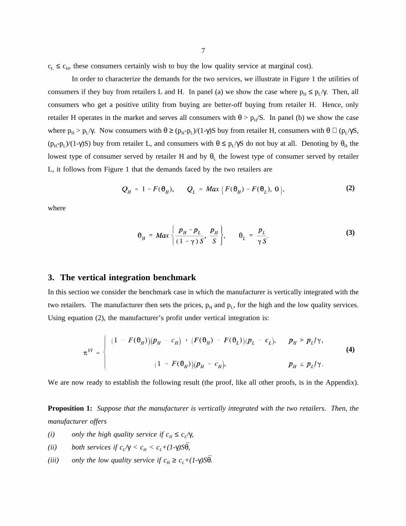
cL ≤ cH, these consumers certainly wish to buy the low quality service at marginal cost).

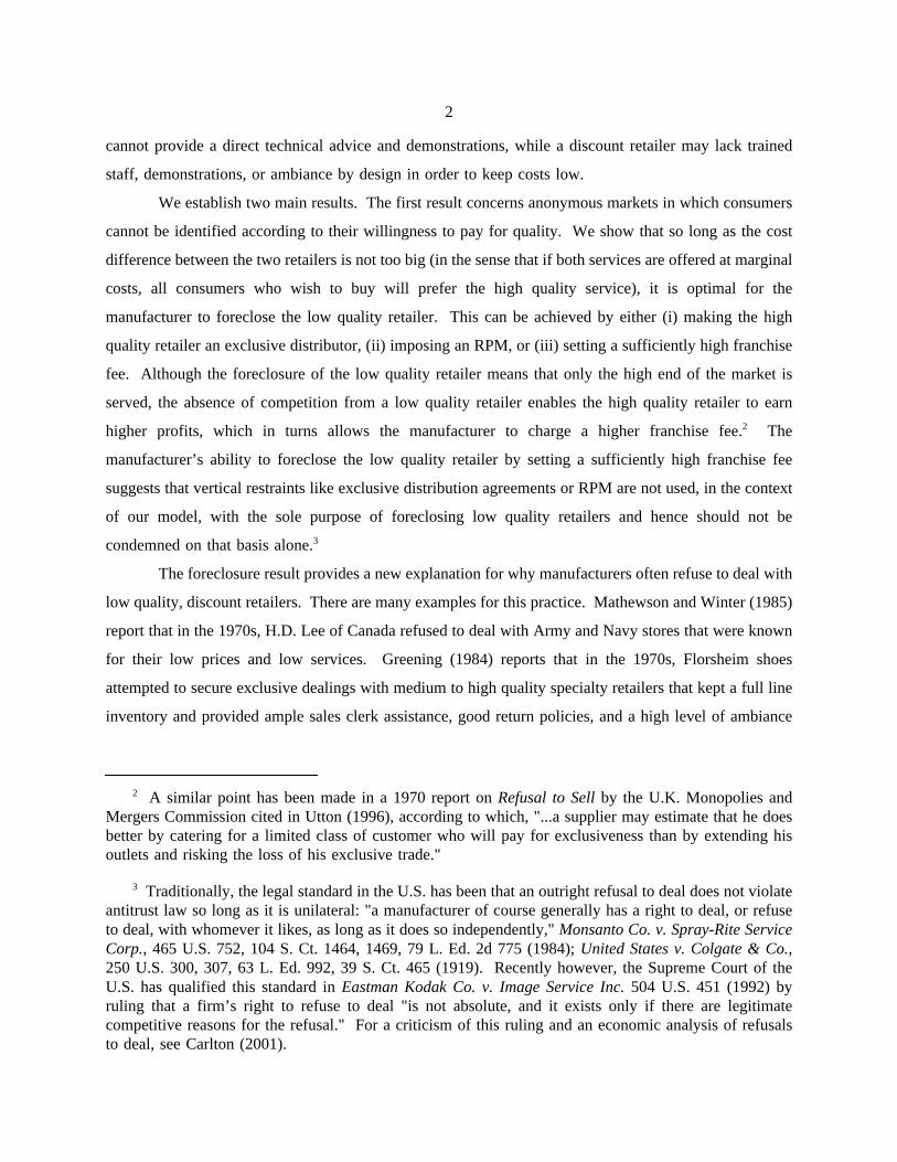
In order to characterize the demands for the two services, we illustrate in Figure 1 the utilities of

consumers if they buy from retailers L and H. In panel (a) we show the case where pH ≤ pL/γ. Then, all

consumers who get a positive utility from buying are better-off buying from retailer H. Hence, only

retailer H operates in the market and serves all consumers with θ > pH/S. In panel (b) we show the case

where pH > pL/γ. Now consumers with θ ≥ (pH-pL)/(1-γ)S buy from retailer H, consumers with θ ∈ (pL/γS,

(pH-pL)/(1-γ)S) buy from retailer L, and consumers with θ ≤ pL/γS do not buy at all. Denoting by θH the

lowest type of consumer served by retailer H and by θL the lowest type of consumer served by retailer

L, it follows from Figure 1 that the demands faced by the two retailers are

where

(2)

(3)

3. The vertical integration benchmark

In this section we consider the benchmark case in which the manufacturer is vertically integrated with the

two retailers. The manufacturer then sets the prices, pH and pL, for the high and the low quality services.

Using equation (2), the manufacturer’s profit under vertical integration is:

We are now ready to establish the following result (the proof, like all other proofs, is in the Appendix).

(4)

Proposition 1: Suppose that the manufacturer is vertically integrated with the two retailers. Then, the

manufacturer offers

(i) only the high quality service if cH ≤ cL/γ,

(ii) both services if cL/γ < cH < cL+(1-γ)Sθ,

(iii) only the low quality service if cH ≥ cL+(1-γ)Sθ.

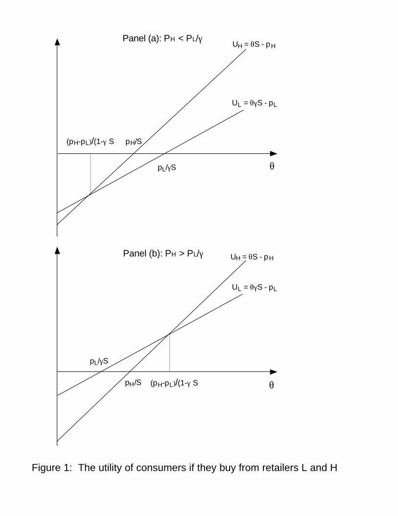
Figure 1: The utility of consumers if they buy from retailers L and H

Panel (a): PH < PL/γUH = θS - pH

UH = θS - pH

θ

UL = θγS - pL

θ

UL = θγS - pL

Panel (b): PH > PL/γ

pL/γS

pL/γS

pH/S

(pH-pL)/(1-γ)S

(pH-pL)/(1-γ)S

pH/S

8

To interpret Proposition 1, note that the vertically integrated manufacturer faces the following

trade-off: by offering both services the manufacturer can discriminate between high and low type

customers and charge the former a high price without losing the business of the latter. But, once the low

quality service is offered, some high type customers who will otherwise buy the high quality service will

now switch to the low quality service. Hence, the manufacturer will not be able to extract as much money

from these consumers as in the case where only the high quality service is offered. Proposition 1 shows

that which effect dominates depends only on the relationship between cH and cL/γ (i.e., the cost-quality

ratios of the two services). Intuitively, note that if both services are offered at marginal costs, consumers

with θ > cH/S obtain a positive utility from buying the high quality service and consumers with θ > cL/γS

obtain a positive utility from buying the low quality service. If cH ≤ cL/γ, then all consumers who wish

to buy, prefer the high quality service over the low quality service. Proposition 1 reveals that in this case,

a vertically integrated manufacturer will only offer the high quality service. The low quality service is

not offered to prevent consumers from switching away from the more profitable high quality service. The

situation is completely reversed when cH ≥ cL+(1-γ)θS. Then, the cost difference between the two services

is so large that all consumers prefer the low quality service if both services are offered at marginal costs.

Now the low quality service is more profitable so the manufacturer does not offer the high quality service

to prevent consumers’ switching. In the intermediate case where cL/γ < cH < cL+(1-γ)θ, consumers with

θ ∈ [cL/γS, (cH-cL)/(1-γ)S] prefer to buy the low quality service when both services are offered at marginal

costs, while consumers with θ > (cH-cL)/(1-γ)S prefer to buy the high quality service. In this case, the

manufacturer offers both services and thereby engages in second degree price discrimination.

In what follows we will assume (unless stated otherwise) that cH ≤ cL/γ. We choose to focus

attention on this case because the salient feature of vertical differentiation (and what distinguishes it from

horizontal differentiation) is that if products/services are equally priced, all consumers rank them in the

same way. However when cL < cH, the two services can no longer be always priced the same, so the

assumption that cH < cL/γ seems like a natural way to preserve the unanimity of consumers regarding the

ranking of the two services.9

Before proceeding, we would like to relate Proposition 1 to existing results in the literature. First,

it is well-known that a monopoly may sometimes prefer to provide only a high quality product rather than

both high and low quality products (see e.g., the example in Mussa and Rosen, 1978). Proposition 1

9 The assumption that cH < cL/γ is analogous to Condition (F) in Shaked and Sutton (1983) which isnecessary and sufficient for the "finiteness property" that says that a vertically differentiated industry withfree entry can have a finite number of active firms.

9

establishes the precise conditions under which this is the case for any distribution of consumers’ types that

has a monotone hazard rate. In particularly, Proposition 1 establishes that when cL = cH, a vertically

integrated manufacturer will only offer the high quality service irrespective of how wide is the support

of the distribution of consumers’ types (we only require that θ > cH/S). This result is in contrast with

Bolton and Bonanno (1988) and Gabszewicz et al (1986), where a vertically integrated manufacturer with

cL = cH = 0 offers only a high quality service when the support of distribution of consumers’ types is

relatively narrow, but otherwise offers both high and low quality services.10 The reason for the difference

is that while we assume that consumers’ preferences are of the Mussa and Rosen (1978) type (see equation

(1)), Bolton and Bonanno and Gabszewicz et al assume that consumers’ preferences are of the Gabszewicz

and Thisse (1979) type, where the utility of a θ type consumer who buys quality q at a price p is U(θ)

= q(θ-p).11 With these preferences and no retail costs, the benefit from introducing both qualities and

discriminating between high and low types consumers outweighs the cost of inducing some high type

customers to switch to the low quality service, if and only if the range of consumers’ types is sufficiently

wide. In our model in contrast, if cL = cH, then the second negative effect always dominates so the

manufacturer will never offer both services, no matter how wide is the range of consumers’ types.12

10 In Gabszewicz et al, the manufacturer can offer n ≥ 2 quality levels. They show that if the supportof the distribution of consumers’ types is sufficiently wide, the manufacturer offers all n quality levels;otherwise the manufacturer offers only the highest available quality.

11 In other words, in our model the preferences of consumers are quasi-linear in income with θrepresenting the marginal utility of quality, whereas in Bolton and Bonanno they are Cobb-Douglas withθ representing the consumers’ income, so θ-p represents the expenditure on "all other goods" while q isthe utility from the consuming the good in question.

12 If retail costs are introduced into the Bolton and Bonanno model, then a vertically integratedmanufacturer may no longer offer both qualities, even if the support of consumers’ type is "sufficiently"wide. To see that, note that Bolton and Bonanno assume that the utility of a type θ consumer is x(θ-pH)if the consumer buys a high quality product, y(θ-pL) if the consumer buys a low quality product, and U0θif the consumer does not buy, where x > y > U0 > 0, and θ is distributed uniformly on the unit interval(the assumption that the lower bound of the support is 0 ensures that the support is "sufficiently" wide).Given these expressions, the lowest types served by retailers L and H, respectively, are θL = ypL/(y-U0)and θH = (xpH-ypL)/(x-y). If the manufacturer offers both services, the resulting optimal prices are

Substituting pH* and pL* into θH and θL, it follows that at the optimum, both services are offered (i.e., θH

> θL) if and only if cH > (x-U0)(2xycL-(x-y)(y-U0))/x(x+y)(y-U0). Although this condition holds when cL

= cH = 0 (the case that Bolton and Bonanno consider), it need not hold in general. For instance, if U0 =

10

Second, using a very similar model to ours, Deneckere and McAfee (1996) show that under certain

conditions, a vertically integrated manufacturer will offer both services even if cL > cH. That is, the

manufacturer will offer a "damaged good" (i.e., a costly inferior version of its product) in order to price

discriminate. The reason why this possibility does not arise in our model is that in Deneckere and

McAfee, the valuation of the damaged good is λ(θ), where λ(θ) ≤ θ and 0 ≤ λ’(θ) < 1. Lemma 3 in their

paper shows that a necessary condition for introducing a damaged good is that λ(θ)/θ is strictly decreasing;

since we assume that λ(θ) = γSθ, λ(θ)/θ is a constant in our paper and hence it is never optimal to

introduce a damaged good.13

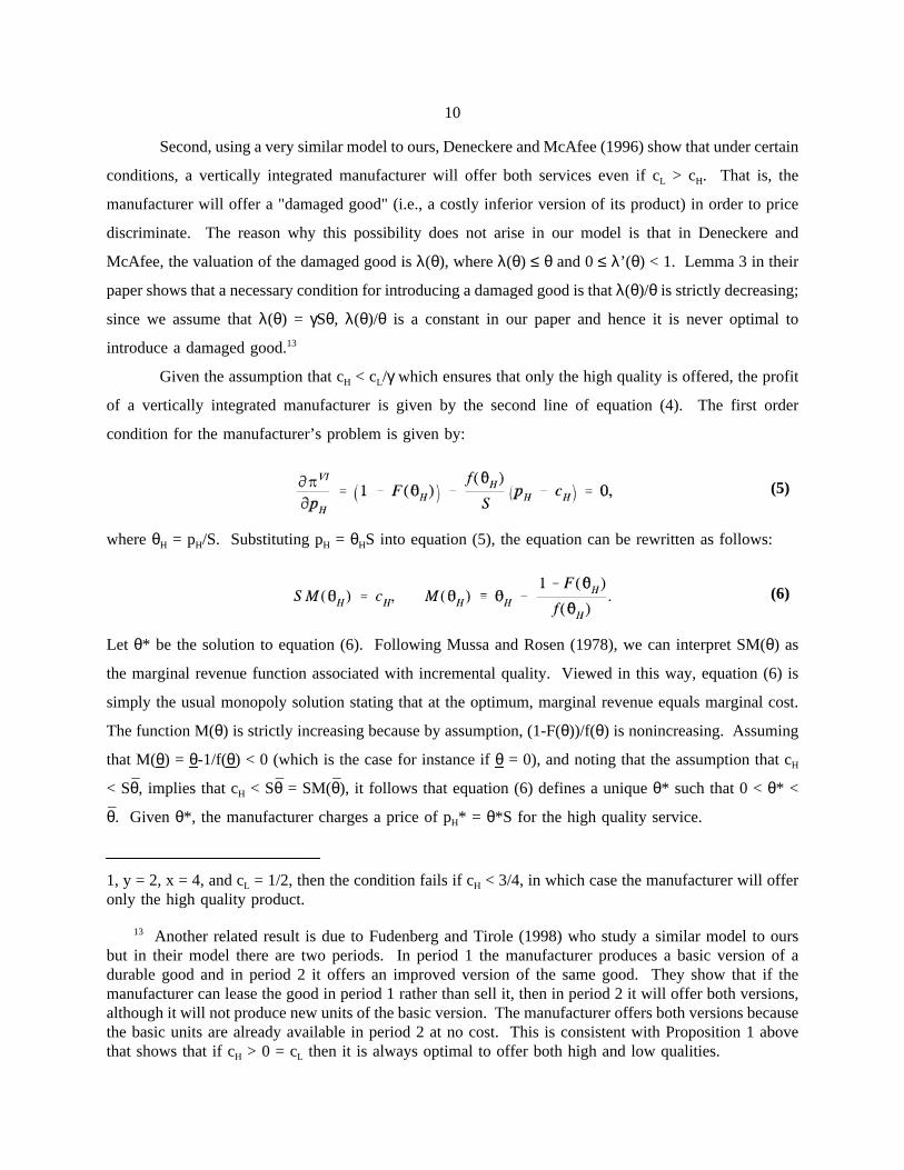
Given the assumption that cH < cL/γ which ensures that only the high quality is offered, the profit

of a vertically integrated manufacturer is given by the second line of equation (4). The first order

condition for the manufacturer’s problem is given by:

where θH = pH/S. Substituting pH = θHS into equation (5), the equation can be rewritten as follows:

(5)

Let θ* be the solution to equation (6). Following Mussa and Rosen (1978), we can interpret SM(θ) as

(6)

the marginal revenue function associated with incremental quality. Viewed in this way, equation (6) is

simply the usual monopoly solution stating that at the optimum, marginal revenue equals marginal cost.

The function M(θ) is strictly increasing because by assumption, (1-F(θ))/f(θ) is nonincreasing. Assuming

that M(θ) = θ-1/f(θ) < 0 (which is the case for instance if θ = 0), and noting that the assumption that cH

< Sθ, implies that cH < Sθ = SM(θ), it follows that equation (6) defines a unique θ* such that 0 < θ* <

θ. Given θ*, the manufacturer charges a price of pH* = θ*S for the high quality service.

1, y = 2, x = 4, and cL = 1/2, then the condition fails if cH < 3/4, in which case the manufacturer will offeronly the high quality product.

13 Another related result is due to Fudenberg and Tirole (1998) who study a similar model to oursbut in their model there are two periods. In period 1 the manufacturer produces a basic version of adurable good and in period 2 it offers an improved version of the same good. They show that if themanufacturer can lease the good in period 1 rather than sell it, then in period 2 it will offer both versions,although it will not produce new units of the basic version. The manufacturer offers both versions becausethe basic units are already available in period 2 at no cost. This is consistent with Proposition 1 abovethat shows that if cH > 0 = cL then it is always optimal to offer both high and low qualities.

11

4. Vertical restraints when the market cannot be vertically segmented

In this section we consider vertical restraints in markets that cannot be vertically segmented according to

the consumers’ willingness to pay for quality. In other words, the manufacturer cannot prevent consumers

from buying from the "wrong" retailer. The main result here is that if the cost difference between the high

and the low quality services is not so big as to reverse the rankings of the two services, the manufacturer

will foreclose retailer L and will only deal with retailer H. Moreover, if the manufacturer can use

franchise fees then it is possible to replicate the vertically integrated outcome. Otherwise the manufacturer

will earn less than in the vertical integration case although retailer L will still be foreclosed.

Given our assumption that cH < cL/γ, Proposition 1 reveals that a vertically integrated manufacturer

will only offer the high quality service and will charge pH* = θ*S. The manufacturer’s profit then is πH*

= (1-F(θ*))(θ*S-cH). If the manufacturer can use two-part tariffs, he can achieve the same profit by

making retailer H an exclusive distributor and setting a 0 wholesale price. Since retailer H is an exclusive

distributor and the wholesale price is 0, the retailer’s profit is given by the second line of equation (4),

so at the optimum, retailer H will charge pH* = θ*S and will earn πH*. The manufacturer can then fully

extract this profit via a franchise fee.

Another way to replicate the vertically integrated outcome is to set a 0 wholesale price, impose

on both services a minimum RPM equal to θ*S, and charge retailer H a franchise fee equal to πH*. Given

this minimum RPM, retailer H will set his price at pH* = θ*S; since retailer L cannot price below pH*,

his market share will be 0. Hence, the resulting outcome is exactly as in the case where retailer H

becomes an exclusive distributor.14 Alternatively, the manufacturer can set the wholesale price equal to

pH*-cH and set a maximum RPM on both services equal to pH*. Once again, only retailer H will be able

to operate in the market and the maximum RPM will be binding. Since under this scheme retailer H

breaks even, the entire industry profits will accrue to the manufacturer.

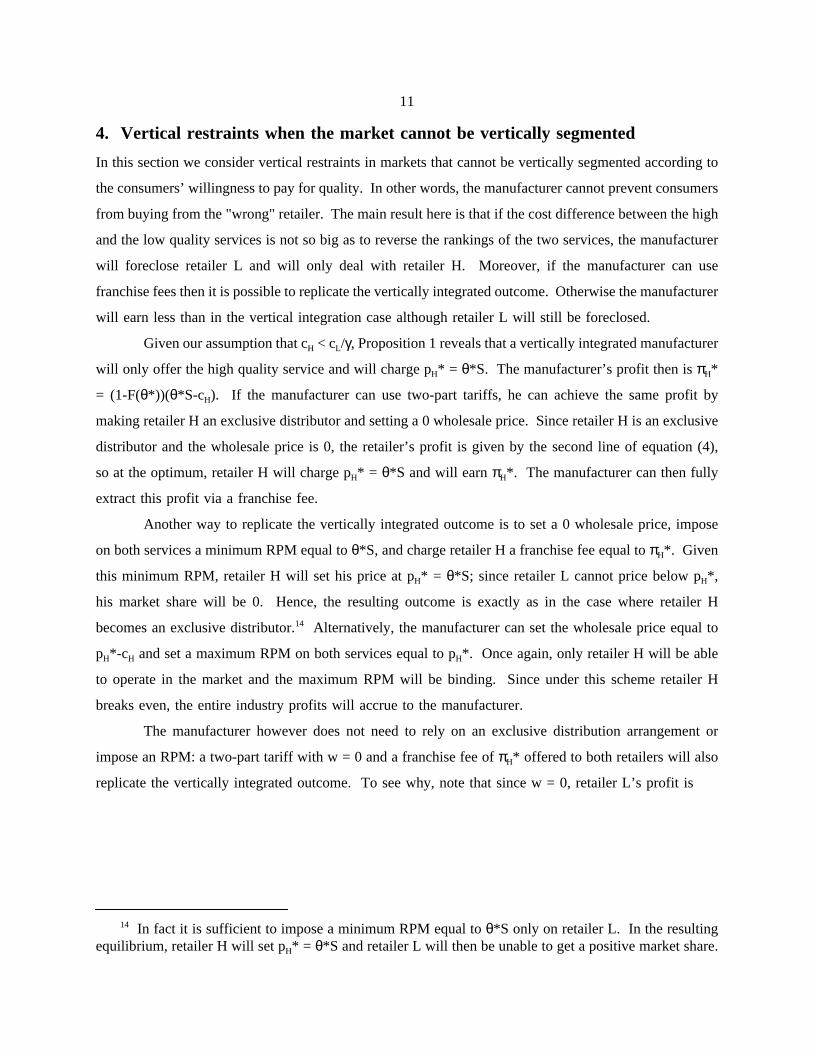
The manufacturer however does not need to rely on an exclusive distribution arrangement or

impose an RPM: a two-part tariff with w = 0 and a franchise fee of πH* offered to both retailers will also

replicate the vertically integrated outcome. To see why, note that since w = 0, retailer L’s profit is

14 In fact it is sufficient to impose a minimum RPM equal to θ*S only on retailer L. In the resultingequilibrium, retailer H will set pH* = θ*S and retailer L will then be unable to get a positive market share.

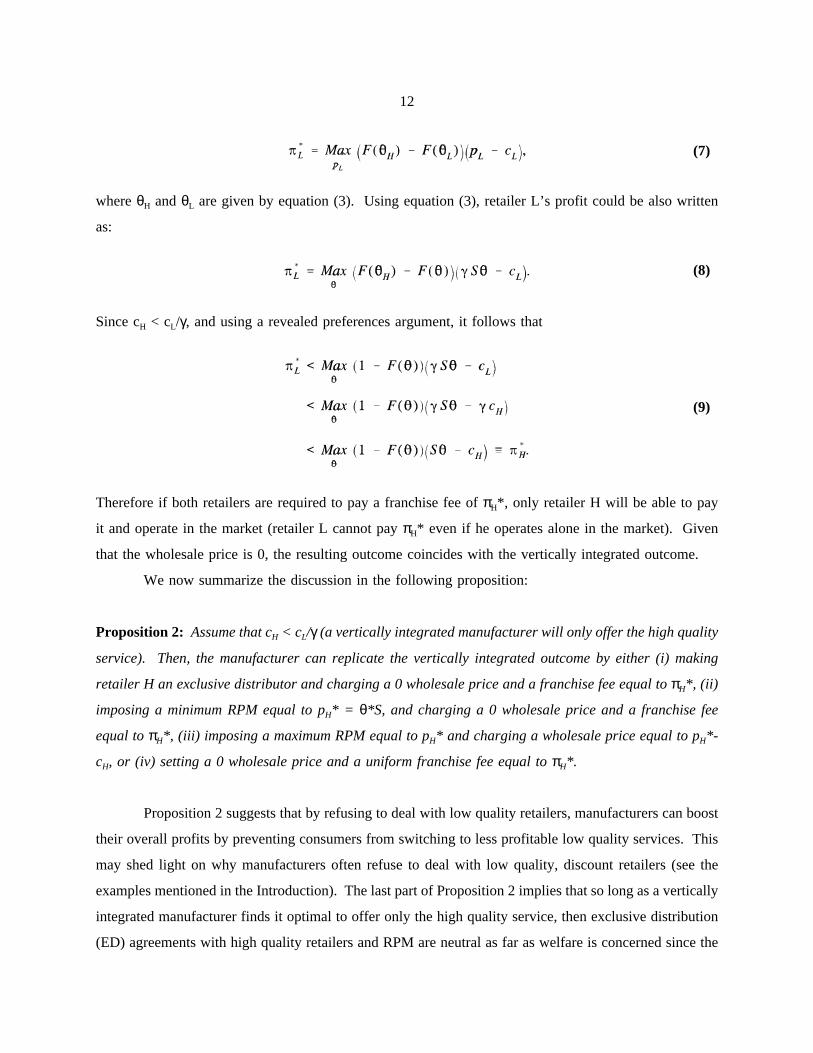
12

where θH and θL are given by equation (3). Using equation (3), retailer L’s profit could be also written

(7)

as:

Since cH < cL/γ, and using a revealed preferences argument, it follows that

(8)

Therefore if both retailers are required to pay a franchise fee of πH*, only retailer H will be able to pay

(9)

it and operate in the market (retailer L cannot pay πH* even if he operates alone in the market). Given

that the wholesale price is 0, the resulting outcome coincides with the vertically integrated outcome.

We now summarize the discussion in the following proposition:

Proposition 2: Assume that cH < cL/γ (a vertically integrated manufacturer will only offer the high quality

service). Then, the manufacturer can replicate the vertically integrated outcome by either (i) making

retailer H an exclusive distributor and charging a 0 wholesale price and a franchise fee equal to πH*, (ii)

imposing a minimum RPM equal to pH* = θ*S, and charging a 0 wholesale price and a franchise fee

equal to πH*, (iii) imposing a maximum RPM equal to pH* and charging a wholesale price equal to pH*-

cH, or (iv) setting a 0 wholesale price and a uniform franchise fee equal to πH*.

Proposition 2 suggests that by refusing to deal with low quality retailers, manufacturers can boost

their overall profits by preventing consumers from switching to less profitable low quality services. This

may shed light on why manufacturers often refuse to deal with low quality, discount retailers (see the

examples mentioned in the Introduction). The last part of Proposition 2 implies that so long as a vertically

integrated manufacturer finds it optimal to offer only the high quality service, then exclusive distribution

(ED) agreements with high quality retailers and RPM are neutral as far as welfare is concerned since the

13

manufacturer can foreclose low quality retailers even without using these arrangements. This suggests in

turn that ED and RPM are not used, in the context of our model, with the sole purpose of foreclosing low

quality retailers and hence should be condemned on that basis alone.

Proposition 2 is somewhat surprising since Bolton and Bonanno (1988, Proposition 3) show in

a closely related model that franchise fees and RPM are insufficient to implement the vertically integrated

outcome. The reason for this difference is that in the Bolton and Bonanno model where cL = cH = 0 and

the range of consumers types is "wide," a vertically integrated manufacturer always prefers to offer both

services. Franchise fees fail to implement the vertically integrated outcome because they induce an

excessive price competition between the two retailers which dissipates some of the profits that the

manufacturer can capture via the franchise fees. In our model, it is optimal to offer only the high quality

service, so franchise fees lead to a foreclosure of retail L and hence prevent dissipative price competition.

As for RPM, then in the Bolton and Bonanno model, both retailers can select the quality of their services.

RPM fails to replicate the vertically integrated outcome because it eliminates the retailers’ incentives to

differentiate their qualities. In our model where qualities are predetermined, there is no such adverse

incentive effect.

Next, we examine the robustness of the foreclosure result with respect to the assumption that the

manufacturer can fully extract the retailers’ profits through franchise fees. In practice, franchise fees might

be substantially smaller than the retailers’ (expected) profits, say due to demand or cost uncertainties and

retailers risk-aversion (see e.g., Rey and Tirole, 1986). One might suspect that if the manufacturer cannot

extract the entire retailers’ profits via franchise fees and cannot impose vertical restraints, then he may

wish to deal with both retailers even if cH < cL/γ (in which case a vertically integrated manufacturer will

offer only the high quality service) in order to expand the size of the market and boost his revenues from

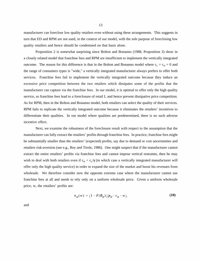
wholesale. We therefore consider now the opposite extreme case where the manufacturer cannot use

franchise fees at all and needs to rely only on a uniform wholesale price. Given a uniform wholesale

price, w, the retailers’ profits are:

and

(10)

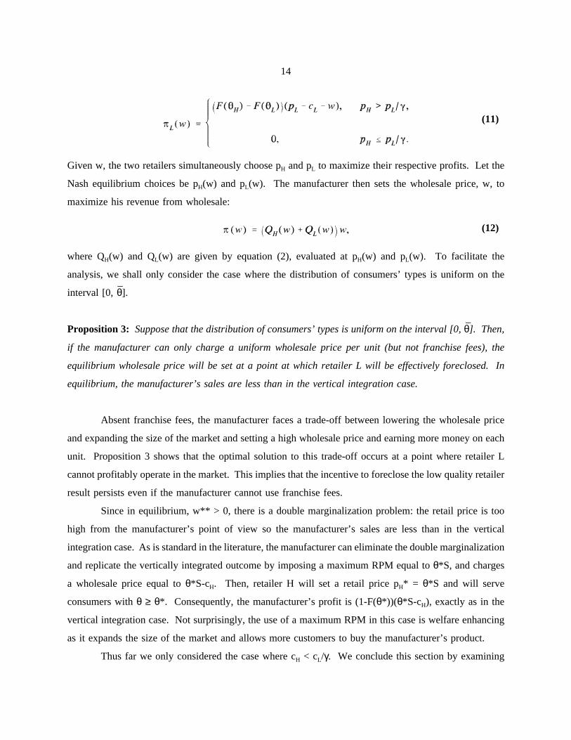
14

Given w, the two retailers simultaneously choose pH and pL to maximize their respective profits. Let the

(11)

Nash equilibrium choices be pH(w) and pL(w). The manufacturer then sets the wholesale price, w, to

maximize his revenue from wholesale:

where QH(w) and QL(w) are given by equation (2), evaluated at pH(w) and pL(w). To facilitate the

(12)

analysis, we shall only consider the case where the distribution of consumers’ types is uniform on the

interval [0, θ].

Proposition 3: Suppose that the distribution of consumers’ types is uniform on the interval [0, θ]. Then,

if the manufacturer can only charge a uniform wholesale price per unit (but not franchise fees), the

equilibrium wholesale price will be set at a point at which retailer L will be effectively foreclosed. In

equilibrium, the manufacturer’s sales are less than in the vertical integration case.

Absent franchise fees, the manufacturer faces a trade-off between lowering the wholesale price

and expanding the size of the market and setting a high wholesale price and earning more money on each

unit. Proposition 3 shows that the optimal solution to this trade-off occurs at a point where retailer L

cannot profitably operate in the market. This implies that the incentive to foreclose the low quality retailer

result persists even if the manufacturer cannot use franchise fees.

Since in equilibrium, w** > 0, there is a double marginalization problem: the retail price is too

high from the manufacturer’s point of view so the manufacturer’s sales are less than in the vertical

integration case. As is standard in the literature, the manufacturer can eliminate the double marginalization

and replicate the vertically integrated outcome by imposing a maximum RPM equal to θ*S, and charges

a wholesale price equal to θ*S-cH. Then, retailer H will set a retail price pH* = θ*S and will serve

consumers with θ ≥ θ*. Consequently, the manufacturer’s profit is (1-F(θ*))(θ*S-cH), exactly as in the

vertical integration case. Not surprisingly, the use of a maximum RPM in this case is welfare enhancing

as it expands the size of the market and allows more customers to buy the manufacturer’s product.

Thus far we only considered the case where cH < cL/γ. We conclude this section by examining

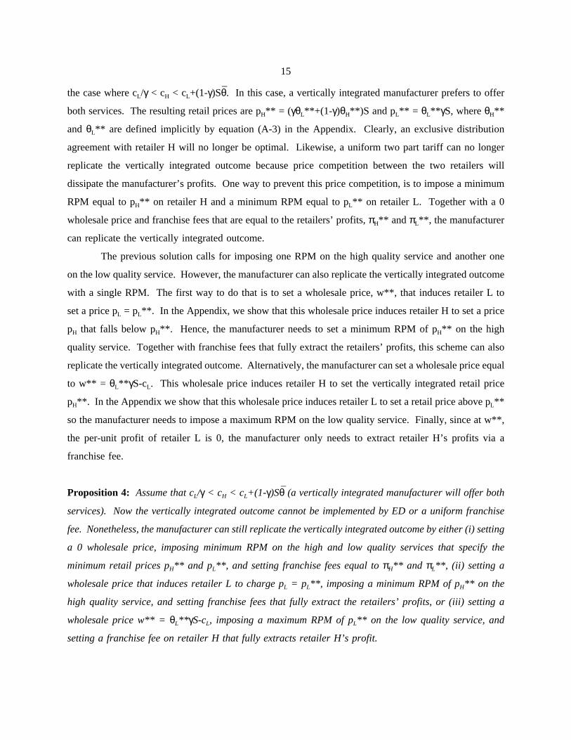
15

the case where cL/γ < cH < cL+(1-γ)Sθ. In this case, a vertically integrated manufacturer prefers to offer

both services. The resulting retail prices are pH** = (γθL**+(1-γ)θH**)S and pL** = θL**γS, where θH**

and θL** are defined implicitly by equation (A-3) in the Appendix. Clearly, an exclusive distribution

agreement with retailer H will no longer be optimal. Likewise, a uniform two part tariff can no longer

replicate the vertically integrated outcome because price competition between the two retailers will

dissipate the manufacturer’s profits. One way to prevent this price competition, is to impose a minimum

RPM equal to pH** on retailer H and a minimum RPM equal to pL** on retailer L. Together with a 0

wholesale price and franchise fees that are equal to the retailers’ profits, πH** and πL**, the manufacturer

can replicate the vertically integrated outcome.

The previous solution calls for imposing one RPM on the high quality service and another one

on the low quality service. However, the manufacturer can also replicate the vertically integrated outcome

with a single RPM. The first way to do that is to set a wholesale price, w**, that induces retailer L to

set a price pL = pL**. In the Appendix, we show that this wholesale price induces retailer H to set a price

pH that falls below pH**. Hence, the manufacturer needs to set a minimum RPM of pH** on the high

quality service. Together with franchise fees that fully extract the retailers’ profits, this scheme can also

replicate the vertically integrated outcome. Alternatively, the manufacturer can set a wholesale price equal

to w** = θL**γS-cL. This wholesale price induces retailer H to set the vertically integrated retail price

pH**. In the Appendix we show that this wholesale price induces retailer L to set a retail price above pL**

so the manufacturer needs to impose a maximum RPM on the low quality service. Finally, since at w**,

the per-unit profit of retailer L is 0, the manufacturer only needs to extract retailer H’s profits via a

franchise fee.

Proposition 4: Assume that cL/γ < cH < cL+(1-γ)Sθ (a vertically integrated manufacturer will offer both

services). Now the vertically integrated outcome cannot be implemented by ED or a uniform franchise

fee. Nonetheless, the manufacturer can still replicate the vertically integrated outcome by either (i) setting

a 0 wholesale price, imposing minimum RPM on the high and low quality services that specify the

minimum retail prices pH** and pL**, and setting franchise fees equal to πH** and πL**, (ii) setting a

wholesale price that induces retailer L to charge pL = pL**, imposing a minimum RPM of pH** on the

high quality service, and setting franchise fees that fully extract the retailers’ profits, or (iii) setting a

wholesale price w** = θL**γS-cL, imposing a maximum RPM of pL** on the low quality service, and

setting a franchise fee on retailer H that fully extracts retailer H’s profit.

16

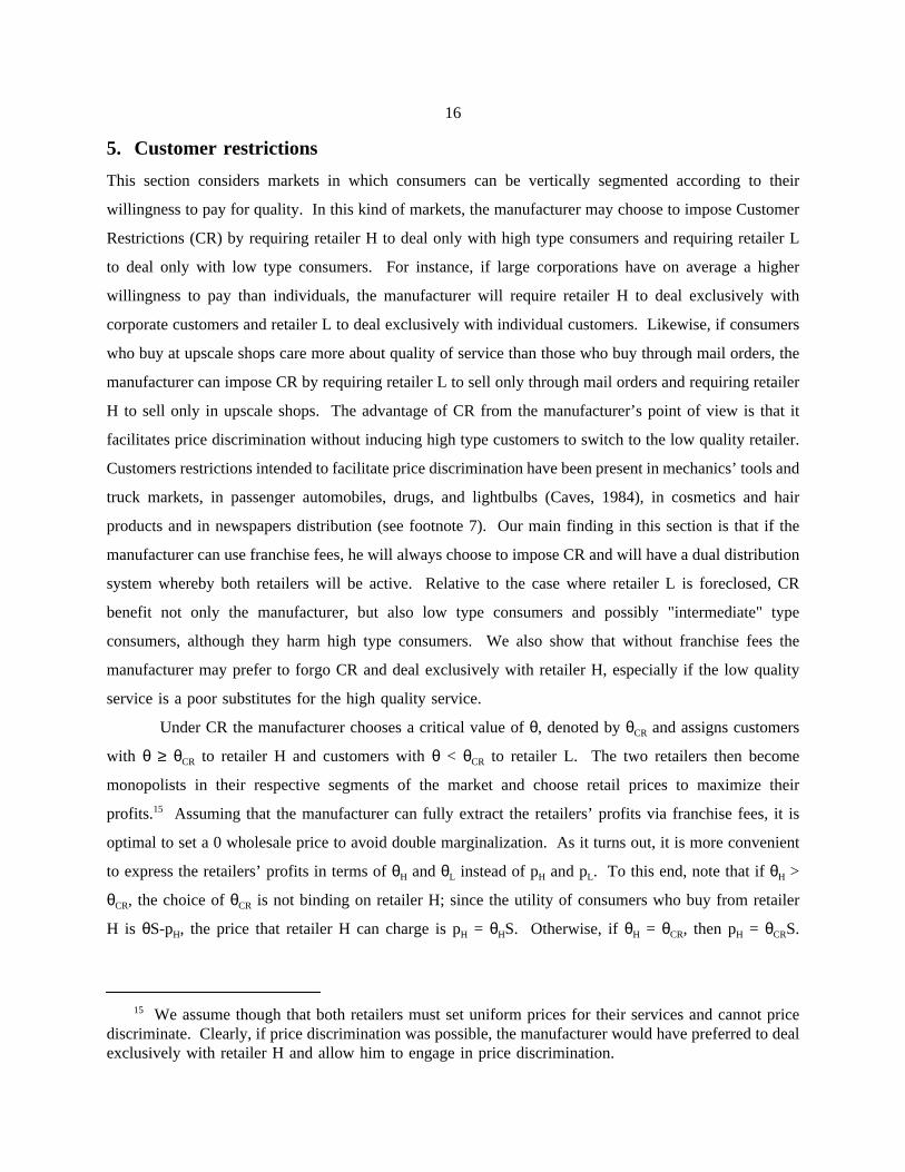
5. Customer restrictions

This section considers markets in which consumers can be vertically segmented according to their

willingness to pay for quality. In this kind of markets, the manufacturer may choose to impose Customer

Restrictions (CR) by requiring retailer H to deal only with high type consumers and requiring retailer L

to deal only with low type consumers. For instance, if large corporations have on average a higher

willingness to pay than individuals, the manufacturer will require retailer H to deal exclusively with

corporate customers and retailer L to deal exclusively with individual customers. Likewise, if consumers

who buy at upscale shops care more about quality of service than those who buy through mail orders, the

manufacturer can impose CR by requiring retailer L to sell only through mail orders and requiring retailer

H to sell only in upscale shops. The advantage of CR from the manufacturer’s point of view is that it

facilitates price discrimination without inducing high type customers to switch to the low quality retailer.

Customers restrictions intended to facilitate price discrimination have been present in mechanics’ tools and

truck markets, in passenger automobiles, drugs, and lightbulbs (Caves, 1984), in cosmetics and hair

products and in newspapers distribution (see footnote 7). Our main finding in this section is that if the

manufacturer can use franchise fees, he will always choose to impose CR and will have a dual distribution

system whereby both retailers will be active. Relative to the case where retailer L is foreclosed, CR

benefit not only the manufacturer, but also low type consumers and possibly "intermediate" type

consumers, although they harm high type consumers. We also show that without franchise fees the

manufacturer may prefer to forgo CR and deal exclusively with retailer H, especially if the low quality

service is a poor substitutes for the high quality service.

Under CR the manufacturer chooses a critical value of θ, denoted by θCR and assigns customers

with θ ≥ θCR to retailer H and customers with θ < θCR to retailer L. The two retailers then become

monopolists in their respective segments of the market and choose retail prices to maximize their

profits.15 Assuming that the manufacturer can fully extract the retailers’ profits via franchise fees, it is

optimal to set a 0 wholesale price to avoid double marginalization. As it turns out, it is more convenient

to express the retailers’ profits in terms of θH and θL instead of pH and pL. To this end, note that if θH >

θCR, the choice of θCR is not binding on retailer H; since the utility of consumers who buy from retailer

H is θS-pH, the price that retailer H can charge is pH = θHS. Otherwise, if θH = θCR, then pH = θCRS.

15 We assume though that both retailers must set uniform prices for their services and cannot pricediscriminate. Clearly, if price discrimination was possible, the manufacturer would have preferred to dealexclusively with retailer H and allow him to engage in price discrimination.

17

Likewise, if 0 ≤ θL < θCR, the utility of consumers who buy from retailer L is θγS-pL, so pL = θLγS. If

θL = θCR, there is no demand for the low quality service. Hence, the profits of the two retailers, gross of

the franchise fees, are

and

(13)

Let θHCR and θL

CR, respectively, be the maximizers of πH(θH) and πL(θL), given θCR. Equation (13) implies

(14)

that θHCR = Max{θCR, θ*}, where θ* is defined implicitly by equation (6). Since θ* is unique, so is θH

CR.

Equation (14) implies that θLCR = Min{θCR, θL*}, where θL* is defined implicitly by the equation γS(θ-

(F(θCR)-F(θ))/f(θ)) = cL. The assumption that 1-F(θ)/f(θ) is nonincreasing implies that the right side of

the equation is strictly increasing so θLCR is unique as well.16 Since the manufacturer can fully extract

the retailers’ profits through the franchise fees, θCR is set to maximize the expression

We denote the maximizer of π(θCR) by θCR*.

(15)

To characterize the equilibrium, note that setting θCR below θ* is dominated from the

16 To see why, note that

If f’(θ) ≥ 0, the derivative is positive as required. If f’(θ) < 0, then since by assumption, 1-F(θ)/f(θ) isnonincreasing, M(θ) ≡ θ - 1-F(θ)/f(θ) is strictly increasing, so as a result,

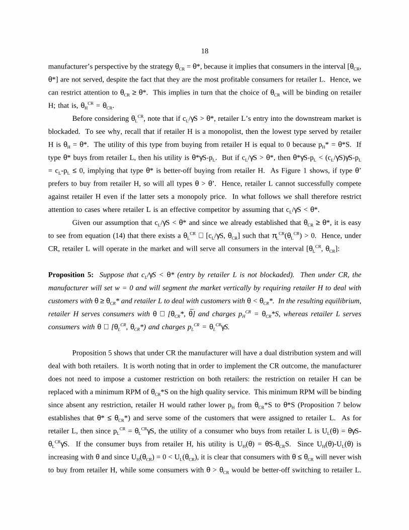
18

manufacturer’s perspective by the strategy θCR = θ*, because it implies that consumers in the interval [θCR,

θ*] are not served, despite the fact that they are the most profitable consumers for retailer L. Hence, we

can restrict attention to θCR ≥ θ*. This implies in turn that the choice of θCR will be binding on retailer

H; that is, θHCR = θCR.

Before considering θLCR, note that if cL/γS > θ*, retailer L’s entry into the downstream market is

blockaded. To see why, recall that if retailer H is a monopolist, then the lowest type served by retailer

H is θH = θ*. The utility of this type from buying from retailer H is equal to 0 because pH* = θ*S. If

type θ* buys from retailer L, then his utility is θ*γS-pL. But if cL/γS > θ*, then θ*γS-pL < (cL/γS)γS-pL

= cL-pL ≤ 0, implying that type θ* is better-off buying from retailer H. As Figure 1 shows, if type θ’

prefers to buy from retailer H, so will all types θ > θ’. Hence, retailer L cannot successfully compete

against retailer H even if the latter sets a monopoly price. In what follows we shall therefore restrict

attention to cases where retailer L is an effective competitor by assuming that cL/γS < θ*.

Given our assumption that cL/γS < θ* and since we already established that θCR ≥ θ*, it is easy

to see from equation (14) that there exists a θLCR ∈ [cL/γS, θCR] such that πL

CR(θLCR) > 0. Hence, under

CR, retailer L will operate in the market and will serve all consumers in the interval [θLCR, θCR]:

Proposition 5: Suppose that cL/γS < θ* (entry by retailer L is not blockaded). Then under CR, the

manufacturer will set w = 0 and will segment the market vertically by requiring retailer H to deal with

customers with θ ≥ θCR* and retailer L to deal with customers with θ < θCR*. In the resulting equilibrium,

retailer H serves consumers with θ ∈ [θCR*, θ] and charges pHCR = θCR*S, whereas retailer L serves

consumers with θ ∈ [θLCR, θCR*) and charges pL

CR = θLCRγS.

Proposition 5 shows that under CR the manufacturer will have a dual distribution system and will

deal with both retailers. It is worth noting that in order to implement the CR outcome, the manufacturer

does not need to impose a customer restriction on both retailers: the restriction on retailer H can be

replaced with a minimum RPM of θCR*S on the high quality service. This minimum RPM will be binding

since absent any restriction, retailer H would rather lower pH from θCR*S to θ*S (Proposition 7 below

establishes that θ* ≤ θCR*) and serve some of the customers that were assigned to retailer L. As for

retailer L, then since pLCR = θL

CRγS, the utility of a consumer who buys from retailer L is UL(θ) = θγS-

θLCRγS. If the consumer buys from retailer H, his utility is UH(θ) = θS-θCRS. Since UH(θ)-UL(θ) is

increasing with θ and since UH(θCR) = 0 < UL(θCR), it is clear that consumers with θ ≤ θCR will never wish

to buy from retailer H, while some consumers with θ > θCR would be better-off switching to retailer L.

19

Hence, given the minimum RPM on retailer H, the manufacturer only needs to worry about retailer L

serving some of retailer’s H customers but never vice versa.

In practice, the manufacturer cannot directly observe the willingness of consumers to pay for

quality and needs to infer it from some observed characteristics of the buyers (e.g., geographic location,

businesses vs. individuals, large vs. small business, etc). If these characteristics are not be perfectly

correlated with θCR*, the manufacturer may end up implementing a θCR which is either above or below

θCR*. However, if the manufacturer errs by setting θCR below θCR*, his profit cannot be lower than it is

absent CR since in the worst case scenario, θCR will be so low that retailer L will be foreclosed, in which

case the manufacturer’s profit is as in Section 4. Hence, from the manufacturer’s point of view, the real

"danger" is to set θCR above θCR*, in which case the sales of retailer H are too low so that the

manufacturer can actually be better-off not relying on CR altogether.

It is worth emphasizing that the result that CR gives rise to a dual distribution system does depend

on the assumption that the manufacturer can charge franchise fees. In the next proposition we show that

absent franchise fees, the manufacturer may raise the wholesale price to the point where retailer L is

effectively foreclosed, at least in the case where the low quality service is a poor substitutes for the high

quality service. To facilitate the analysis we only consider cases where the distribution of consumers’

types is uniform on the interval [0, θ].

Proposition 6: Suppose that the distribution of consumers’ types is uniform on the interval [0, θ] and

assume that the manufacturer cannot use franchise fees. Then if γ < 2/5 (the low quality service is a poor

substitutes for the high quality service) the manufacturer will raise the wholesale price to the point where

retailer L will be effectively foreclosed.

As noted above, in the absence of franchise fees, the choice of a wholesale price involves a

tradeoff between raising the wholesale price to earn more money on each unit sold, and lowering the

wholesale price to boost sales. Intuitively, when γ is small, the gain in sales from lowering the wholesale

price is small so the manufacturer raises the wholesale price up to the point where retailer L cannot

successfully compete with retailer H.

We now return to the case where the manufacturer can use franchise fees and wish to compare

the outcome under CR with the outcomes under two-part tariffs, ED, and RPM, characterized in

Proposition 2. We begin by characterizing θCR*. Given that θHCR = θCR and using the envelop theorem,

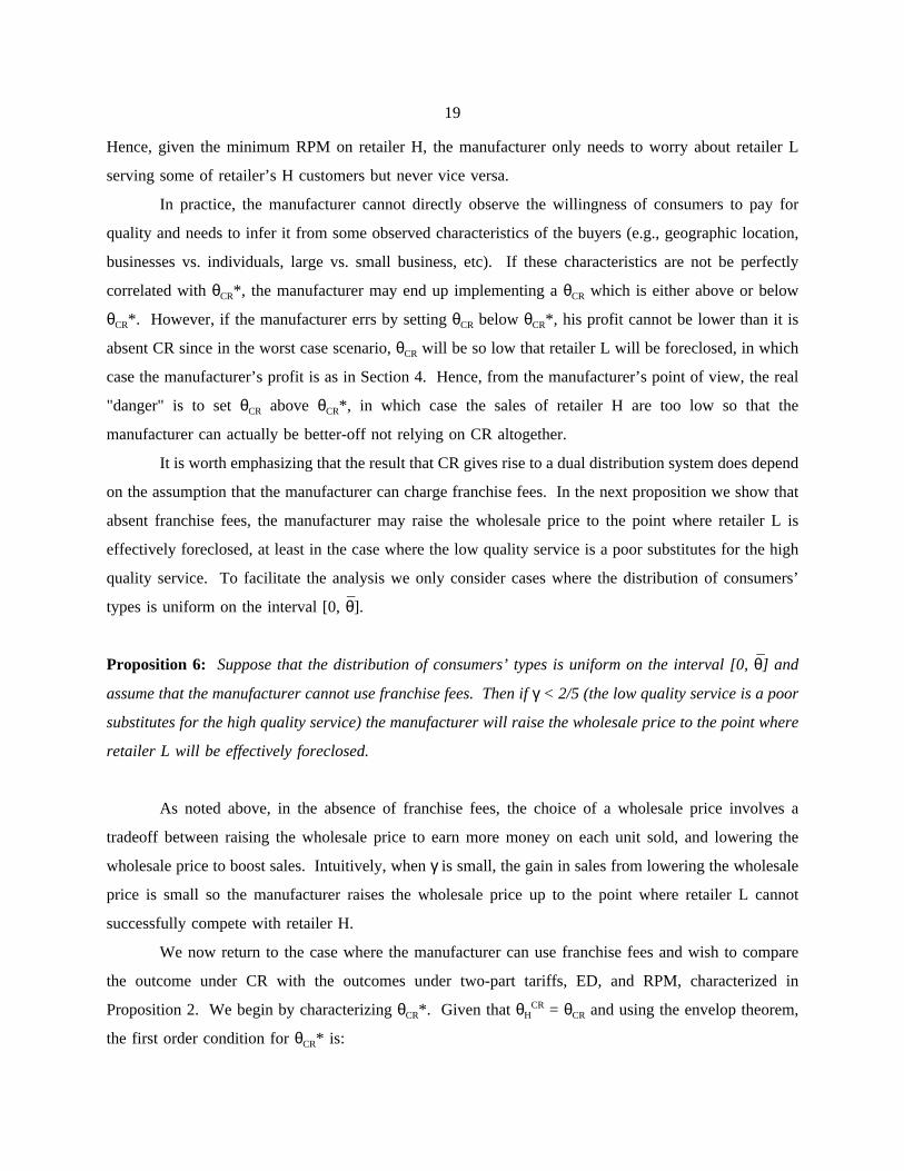
the first order condition for θCR* is:

20

Using the definition of M(θ), this condition can also be written as follows:

(16)

Since M(θ) is strictly increasing, θCR* is defined uniquely. Noting that θLCRγS-cL is the equilibrium price-

(17)

cost margin of retailer L (and hence is nonnegative), it follows that the right side of equation (17) is at

least as large as the right side of equation (6). Hence, θ* ≤ θCR*, so retailer H serves fewer consumers

under CR than under two-part tariffs, ED, or an RPM. Moreover, θCR* < θ, otherwise retailer H is

foreclosed; this however cannot arise in equilibrium as the manufacturer would rather foreclose retailer

L, say by setting θCR* = 0, and deal exclusively with retailer H.

Although retailer H serves fewer consumers than under optimal two-part tariffs, ED, and RPM,

the total size of the market may nonetheless increase under CR because retailer L is also active in the

market. We establish this result by comparing θLCR which is the lowest type that still buys under CR and

θ* which is the lowest type served absent CR:

Proposition 7: Suppose that cL/γS < θ* (entry by retailer L is not blockaded). Then θLCR < θ* ≤ θCR*.

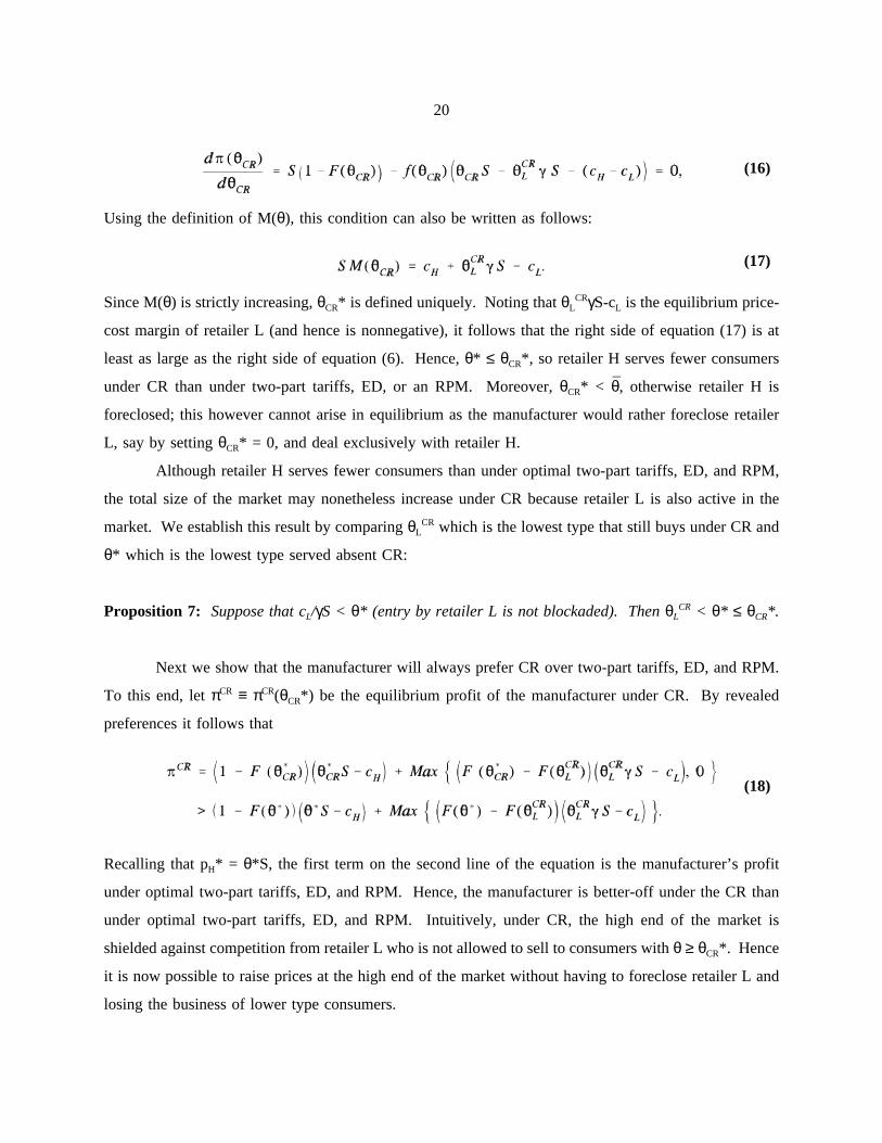
Next we show that the manufacturer will always prefer CR over two-part tariffs, ED, and RPM.

To this end, let πCR ≡ πCR(θCR*) be the equilibrium profit of the manufacturer under CR. By revealed

preferences it follows that

Recalling that pH* = θ*S, the first term on the second line of the equation is the manufacturer’s profit

(18)

under optimal two-part tariffs, ED, and RPM. Hence, the manufacturer is better-off under the CR than

under optimal two-part tariffs, ED, and RPM. Intuitively, under CR, the high end of the market is

shielded against competition from retailer L who is not allowed to sell to consumers with θ ≥ θCR*. Hence

it is now possible to raise prices at the high end of the market without having to foreclose retailer L and

losing the business of lower type consumers.

21

The impact of CR on consumers is more complex since we need to distinguish between at least

three groups of consumers. First, at the top end of the market, consumers with θ ∈ [θCR*, θ], are served

by retailer H under both CR, optimal two-part tariffs, ED, and RPM. But since pHCR > pH*, this group

of consumers is made worse-off under CR.

Second, low type consumers with θ ∈ [θLCR, θ*] are not served at all under two-part tariffs, ED,

and RPM, but are served under CR by retailer L. Hence, CR benefits consumers in the second group.

Third, consumers with θ ∈ [θ*, θCR*] are served by retailer H under optimal two-part tariffs, ED,

and RPM, pay pH* = θ*S, and obtain a utility of U*(θ) = θS-θ*S. Under CR in contrast, these consumers

are served by retailer L, pay pLCR = θL

CRγS, and obtain a utility of UCR(θ) = θγS-θLCRγS. Since U*(θ*) =

0, CR surely benefits consumers with θ close to θ*. However, since UCR(θ)-U*(θ) is decreasing with θ,

consumers with θ close to θCR might be hurt by CR. To examine this issue, note that at the top end of

the second group, UCR(θCR)-U*(θCR) = (θ*-γθLCR-(1-γ)θCR)S. If θ* > γθL

CR+(1-γ)θCR, then UCR(θCR) >

U*(θCR) > 0 implying that CR benefits all consumers in the second group; otherwise there is some cutoff

level, θ ∈ [θ*, θCR*], such that CR benefits consumers with θ ∈ [θ*, θ] and hurts consumers with θ ∈

[θ, θCR*]. We summarize this discussion as follows:

Proposition 8: The manufacturer always prefers CR over two-part tariffs, ED or RPM. As for

consumers, relative to optimal two-part tariffs, ED, and RPM,

(i) consumers with θ ∈ [θCR*, θ] are hurt by CR,

(ii) consumers with θ ∈ [θLCR, θ*] benefit from CR, and

(iii) consumers with θ ∈ [θ*, θCR*] benefit from CR if θ* > γθLCR+(1-γ)θCR; otherwise, there exists

some cutoff level, θ ∈ [θ*, θCR], such that CR benefits consumers with θ ∈ [θ*, θ] and hurts

consumers with θ ∈ [θ, θCR].

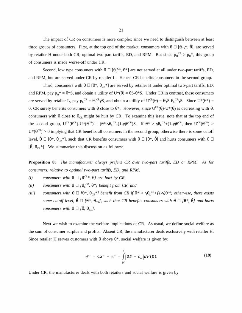
Next we wish to examine the welfare implications of CR. As usual, we define social welfare as

the sum of consumer surplus and profits. Absent CR, the manufacturer deals exclusively with retailer H.

Since retailer H serves customers with θ above θ*, social welfare is given by:

Under CR, the manufacturer deals with both retailers and social welfare is given by

(19)

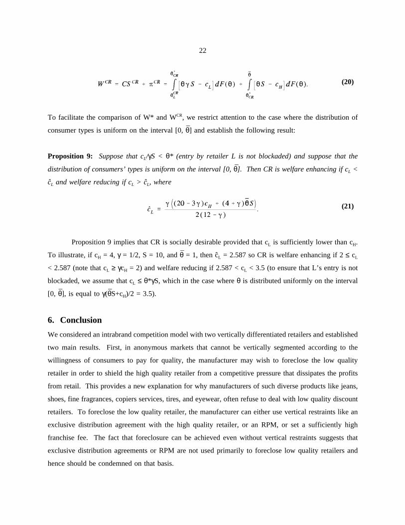
22

To facilitate the comparison of W* and WCR, we restrict attention to the case where the distribution of

(20)

consumer types is uniform on the interval [0, θ] and establish the following result:

Proposition 9: Suppose that cL/γS < θ* (entry by retailer L is not blockaded) and suppose that the

distribution of consumers’ types is uniform on the interval [0, θ]. Then CR is welfare enhancing if cL <

cL and welfare reducing if cL > cL, where

(21)

Proposition 9 implies that CR is socially desirable provided that cL is sufficiently lower than cH.

To illustrate, if cH = 4, γ = 1/2, S = 10, and θ = 1, then cL = 2.587 so CR is welfare enhancing if 2 ≤ cL

< 2.587 (note that cL ≥ γcH = 2) and welfare reducing if 2.587 < cL < 3.5 (to ensure that L’s entry is not

blockaded, we assume that cL ≤ θ*γS, which in the case where θ is distributed uniformly on the interval

[0, θ], is equal to γ(θS+cH)/2 = 3.5).

6. Conclusion

We considered an intrabrand competition model with two vertically differentiated retailers and established

two main results. First, in anonymous markets that cannot be vertically segmented according to the

willingness of consumers to pay for quality, the manufacturer may wish to foreclose the low quality

retailer in order to shield the high quality retailer from a competitive pressure that dissipates the profits

from retail. This provides a new explanation for why manufacturers of such diverse products like jeans,

shoes, fine fragrances, copiers services, tires, and eyewear, often refuse to deal with low quality discount

retailers. To foreclose the low quality retailer, the manufacturer can either use vertical restraints like an

exclusive distribution agreement with the high quality retailer, or an RPM, or set a sufficiently high

franchise fee. The fact that foreclosure can be achieved even without vertical restraints suggests that

exclusive distribution agreements or RPM are not used primarily to foreclose low quality retailers and

hence should be condemned on that basis.

23

We then showed that in markets that can be vertically segmented according to the willingness of

consumers to pay for quality, the manufacturer will impose customer restrictions by requiring the low

quality retailer to serve consumers whose willingness to pay for quality is below some threshold while

requiring the high quality retailer to serve consumers whose willingness to pay for quality is above the

threshold. The advantage of this restriction is that it shields the high quality retailer from competition

from the low quality retailer, while still enabling the manufacturer to reach the low end of the market

through the low quality retailer. Consequently, customer restrictions allow more consumers to be served

and may therefore enhance welfare especially if the cost of the low quality retailer is low.

24

Appendix

Following are the proofs of Proposition 1, 3, 4, 6, 7, and 9.

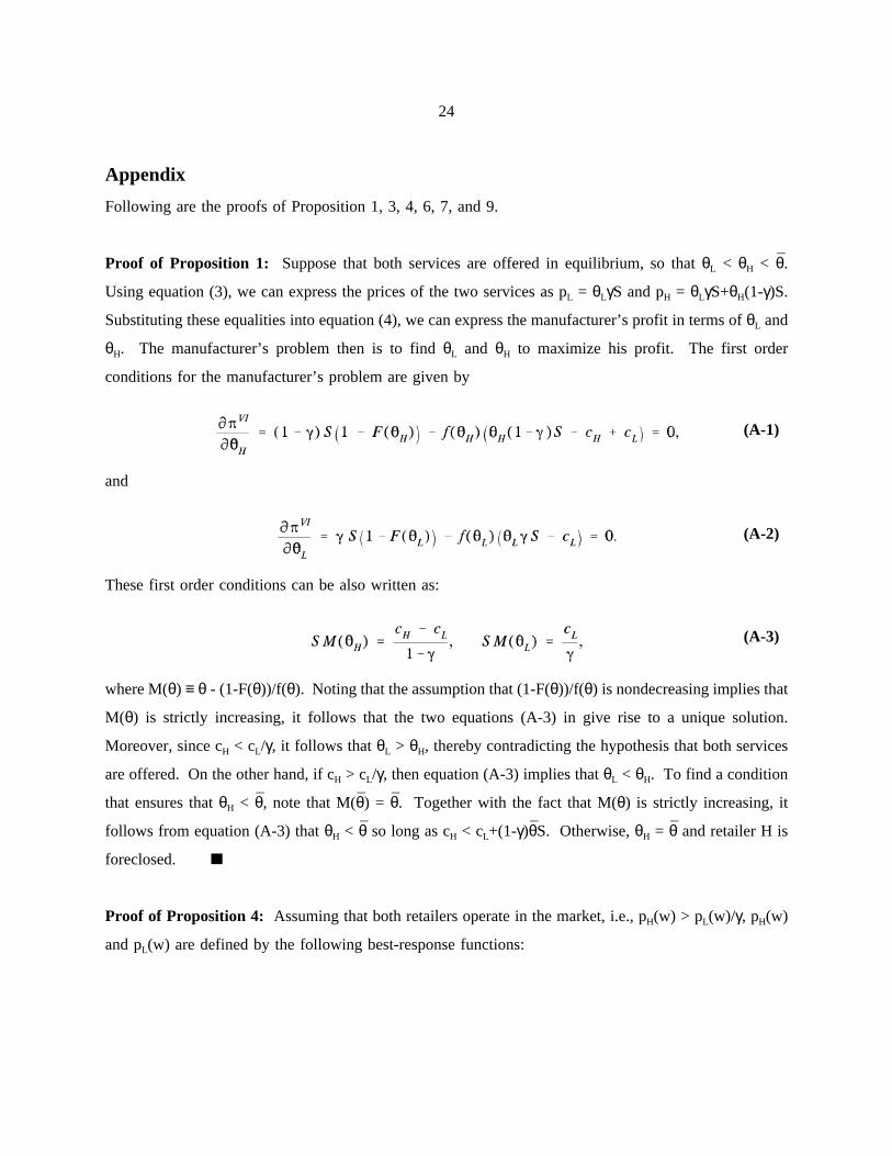
Proof of Proposition 1: Suppose that both services are offered in equilibrium, so that θL < θH < θ.

Using equation (3), we can express the prices of the two services as pL = θLγS and pH = θLγS+θH(1-γ)S.

Substituting these equalities into equation (4), we can express the manufacturer’s profit in terms of θL and

θH. The manufacturer’s problem then is to find θL and θH to maximize his profit. The first order

conditions for the manufacturer’s problem are given by

and

(A-1)

These first order conditions can be also written as:

(A-2)

where M(θ) ≡ θ - (1-F(θ))/f(θ). Noting that the assumption that (1-F(θ))/f(θ) is nondecreasing implies that

(A-3)

M(θ) is strictly increasing, it follows that the two equations (A-3) in give rise to a unique solution.

Moreover, since cH < cL/γ, it follows that θL > θH, thereby contradicting the hypothesis that both services

are offered. On the other hand, if cH > cL/γ, then equation (A-3) implies that θL < θH. To find a condition

that ensures that θH < θ, note that M(θ) = θ. Together with the fact that M(θ) is strictly increasing, it

follows from equation (A-3) that θH < θ so long as cH < cL+(1-γ)θS. Otherwise, θH = θ and retailer H is

foreclosed.

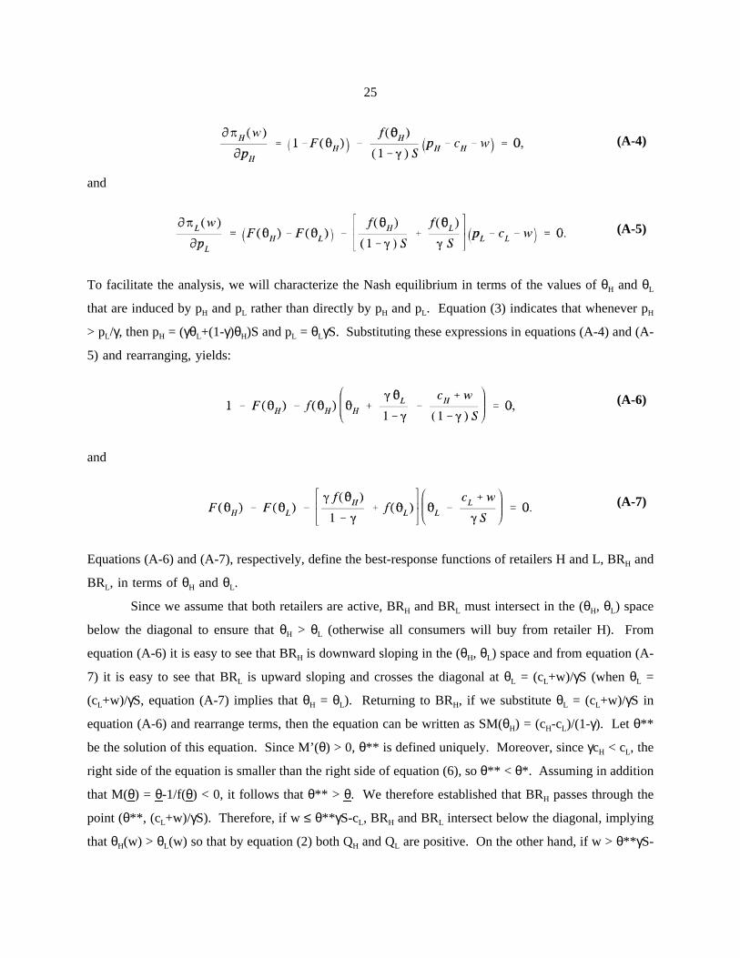
Proof of Proposition 4: Assuming that both retailers operate in the market, i.e., pH(w) > pL(w)/γ, pH(w)

and pL(w) are defined by the following best-response functions:

25

and

(A-4)

To facilitate the analysis, we will characterize the Nash equilibrium in terms of the values of θH and θL

(A-5)

that are induced by pH and pL rather than directly by pH and pL. Equation (3) indicates that whenever pH

> pL/γ, then pH = (γθL+(1-γ)θH)S and pL = θLγS. Substituting these expressions in equations (A-4) and (A-

5) and rearranging, yields:

and

(A-6)

Equations (A-6) and (A-7), respectively, define the best-response functions of retailers H and L, BRH and

(A-7)

BRL, in terms of θH and θL.

Since we assume that both retailers are active, BRH and BRL must intersect in the (θH, θL) space

below the diagonal to ensure that θH > θL (otherwise all consumers will buy from retailer H). From

equation (A-6) it is easy to see that BRH is downward sloping in the (θH, θL) space and from equation (A-

7) it is easy to see that BRL is upward sloping and crosses the diagonal at θL = (cL+w)/γS (when θL =

(cL+w)/γS, equation (A-7) implies that θH = θL). Returning to BRH, if we substitute θL = (cL+w)/γS in

equation (A-6) and rearrange terms, then the equation can be written as SM(θH) = (cH-cL)/(1-γ). Let θ**

be the solution of this equation. Since M’(θ) > 0, θ** is defined uniquely. Moreover, since γcH < cL, the

right side of the equation is smaller than the right side of equation (6), so θ** < θ*. Assuming in addition

that M(θ) = θ-1/f(θ) < 0, it follows that θ** > θ. We therefore established that BRH passes through the

point (θ**, (cL+w)/γS). Therefore, if w ≤ θ**γS-cL, BRH and BRL intersect below the diagonal, implying

that θH(w) > θL(w) so that by equation (2) both QH and QL are positive. On the other hand, if w > θ**γS-

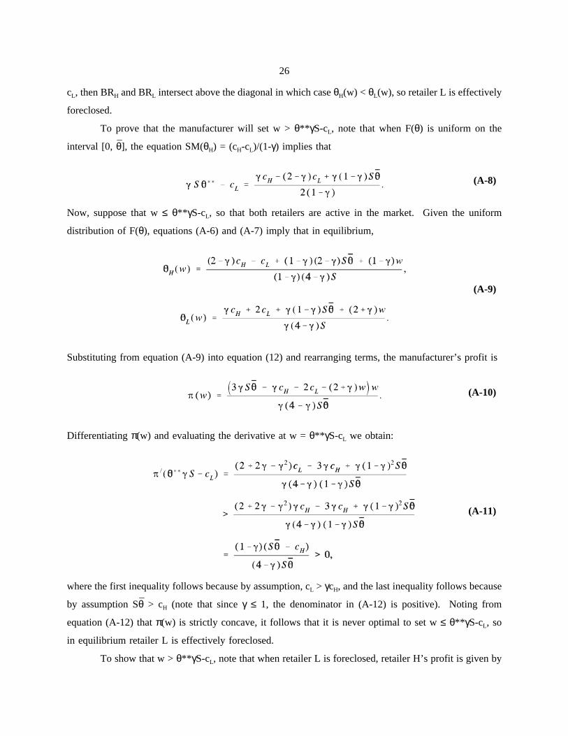
26

cL, then BRH and BRL intersect above the diagonal in which case θH(w) < θL(w), so retailer L is effectively

foreclosed.

To prove that the manufacturer will set w > θ**γS-cL, note that when F(θ) is uniform on the

interval [0, θ], the equation SM(θH) = (cH-cL)/(1-γ) implies that

Now, suppose that w ≤ θ**γS-cL, so that both retailers are active in the market. Given the uniform

(A-8)

distribution of F(θ), equations (A-6) and (A-7) imply that in equilibrium,

Substituting from equation (A-9) into equation (12) and rearranging terms, the manufacturer’s profit is

(A-9)

Differentiating π(w) and evaluating the derivative at w = θ**γS-cL we obtain:

(A-10)

where the first inequality follows because by assumption, cL > γcH, and the last inequality follows because

(A-11)

by assumption Sθ > cH (note that since γ ≤ 1, the denominator in (A-12) is positive). Noting from

equation (A-12) that π(w) is strictly concave, it follows that it is never optimal to set w ≤ θ**γS-cL, so

in equilibrium retailer L is effectively foreclosed.

To show that w > θ**γS-cL, note that when retailer L is foreclosed, retailer H’s profit is given by

27

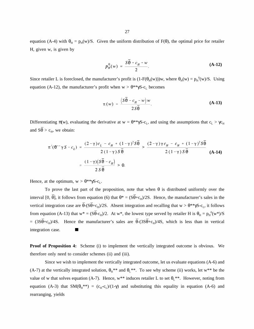
equation (A-4) with θH = pH(w)/S. Given the uniform distribution of F(θ), the optimal price for retailer

H, given w, is given by

Since retailer L is foreclosed, the manufacturer’s profit is (1-F(θH(w)))w, where θH(w) = pH0(w)/S. Using

(A-12)

equation (A-12), the manufacturer’s profit when w > θ**γS-cL becomes

Differentiating π(w), evaluating the derivative at w = θ**γS-cL, and using the assumptions that cL > γcH

(A-13)

and Sθ > cH, we obtain:

Hence, at the optimum, w > θ**γS-cL.

(A-14)

To prove the last part of the proposition, note that when θ is distributed uniformly over the

interval [0, θ], it follows from equation (6) that θ* = (Sθ+cH)/2S. Hence, the manufacturer’s sales in the

vertical integration case are θ-(Sθ+cH)/2S. Absent integration and recalling that w > θ**γS-cL, it follows

from equation (A-13) that w* = (Sθ-cH)/2. At w*, the lowest type served by retailer H is θH = pH0(w*)/S

= (3Sθ+cH)/4S. Hence the manufacturer’s sales are θ-(3Sθ+cH)/4S, which is less than in vertical

integration case.

Proof of Proposition 4: Scheme (i) to implement the vertically integrated outcome is obvious. We

therefore only need to consider schemes (ii) and (iii).

Since we wish to implement the vertically integrated outcome, let us evaluate equations (A-6) and

(A-7) at the vertically integrated solution, θH** and θL**. To see why scheme (ii) works, let w** be the

value of w that solves equation (A-7). Hence, w** induces retailer L to set θL**. However, noting from

equation (A-3) that SM(θH**) = (cH-cL)/(1-γ) and substituting this equality in equation (A-6) and

rearranging, yields

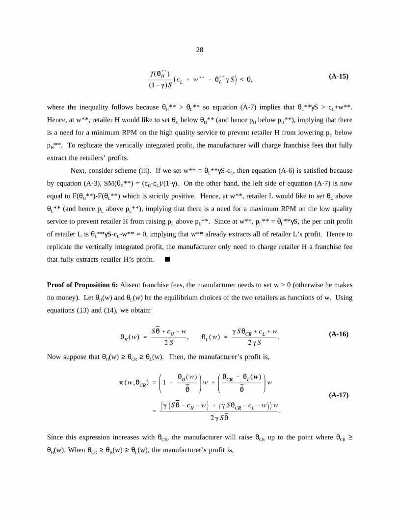
28

where the inequality follows because θH** > θL** so equation (A-7) implies that θL**γS > cL+w**.

(A-15)

Hence, at w**, retailer H would like to set θH below θH** (and hence pH below pH**), implying that there

is a need for a minimum RPM on the high quality service to prevent retailer H from lowering pH below

pH**. To replicate the vertically integrated profit, the manufacturer will charge franchise fees that fully

extract the retailers’ profits.

Next, consider scheme (iii). If we set w** = θL**γS-cL, then equation (A-6) is satisfied because

by equation (A-3), SM(θH**) = (cH-cL)/(1-γ). On the other hand, the left side of equation (A-7) is now

equal to F(θH**)-F(θL**) which is strictly positive. Hence, at w**, retailer L would like to set θL above

θL** (and hence pL above pL**), implying that there is a need for a maximum RPM on the low quality

service to prevent retailer H from raising pL above pL**. Since at w**, pL** = θL**γS, the per unit profit

of retailer L is θL**γS-cL-w** = 0, implying that w** already extracts all of retailer L’s profit. Hence to

replicate the vertically integrated profit, the manufacturer only need to charge retailer H a franchise fee

that fully extracts retailer H’s profit.

Proof of Proposition 6: Absent franchise fees, the manufacturer needs to set w > 0 (otherwise he makes

no money). Let θH(w) and θL(w) be the equilibrium choices of the two retailers as functions of w. Using

equations (13) and (14), we obtain:

Now suppose that θH(w) ≥ θCR ≥ θL(w). Then, the manufacturer’s profit is,

(A-16)

Since this expression increases with θCR, the manufacturer will raise θCR up to the point where θCR ≥

(A-17)

θH(w). When θCR ≥ θH(w) ≥ θL(w), the manufacturer’s profit is,

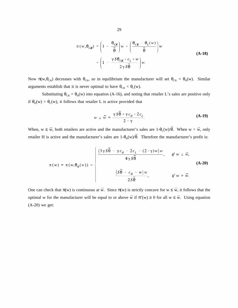
29

Now π(w,θCR) decreases with θCR, so in equilibrium the manufacturer will set θCR = θH(w). Similar

(A-18)

arguments establish that it is never optimal to have θCR < θL(w).

Substituting θCR = θH(w) into equation (A-16), and noting that retailer L’s sales are positive only

if θH(w) > θL(w), it follows that retailer L is active provided that

When, w ≤ w, both retailers are active and the manufacturer’s sales are 1-θL(w)/θ. When w > w, only

(A-19)

retailer H is active and the manufacturer’s sales are 1-θH(w)/θ. Therefore the manufacturer’s profit is:

One can check that π(w) is continuous at w. Since π(w) is strictly concave for w ≤ w, it follows that the

(A-20)

optimal w for the manufacturer will be equal to or above w if π’(w) ≥ 0 for all w ≤ w. Using equation

(A-20) we get:

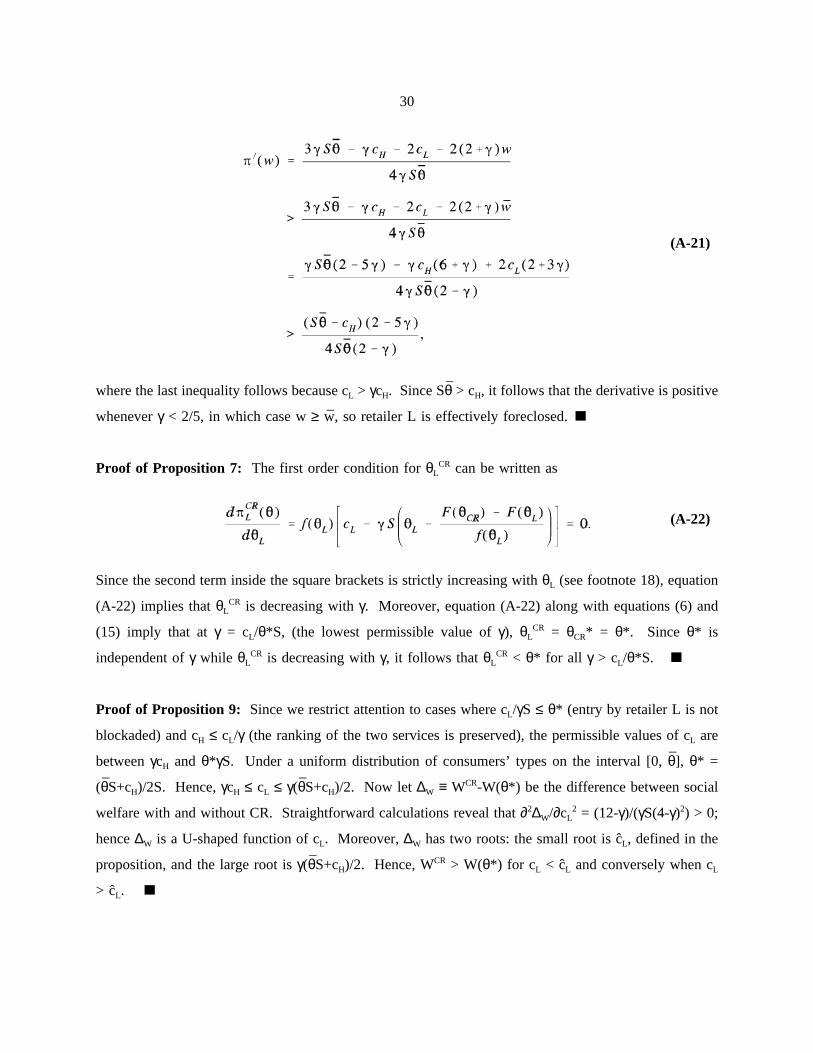
30

where the last inequality follows because cL > γcH. Since Sθ > cH, it follows that the derivative is positive

(A-21)

whenever γ < 2/5, in which case w ≥ w, so retailer L is effectively foreclosed.

Proof of Proposition 7: The first order condition for θLCR can be written as

Since the second term inside the square brackets is strictly increasing with θL (see footnote 18), equation

(A-22)

(A-22) implies that θLCR is decreasing with γ. Moreover, equation (A-22) along with equations (6) and

(15) imply that at γ = cL/θ*S, (the lowest permissible value of γ), θLCR = θCR* = θ*. Since θ* is

independent of γ while θLCR is decreasing with γ, it follows that θL

CR < θ* for all γ > cL/θ*S.

Proof of Proposition 9: Since we restrict attention to cases where cL/γS ≤ θ* (entry by retailer L is not

blockaded) and cH ≤ cL/γ (the ranking of the two services is preserved), the permissible values of cL are

between γcH and θ*γS. Under a uniform distribution of consumers’ types on the interval [0, θ], θ* =

(θS+cH)/2S. Hence, γcH ≤ cL ≤ γ(θS+cH)/2. Now let ∆W ≡ WCR-W(θ*) be the difference between social

welfare with and without CR. Straightforward calculations reveal that ∂2∆W/∂cL2 = (12-γ)/(γS(4-γ)2) > 0;

hence ∆W is a U-shaped function of cL. Moreover, ∆W has two roots: the small root is cL, defined in the

proposition, and the large root is γ(θS+cH)/2. Hence, WCR > W(θ*) for cL < cL and conversely when cL

> cL.

31

References

Baxter W. (1984), "Vertical Restraints - Half Slave, Half Free," Antitrust Law Journal, 52, 743-754.

Bolton P. and G. Bonanno (1988), "Vertical Restraints in A Model of Vertical Differentiation," Quarterly

Journal of Economics, 103, 555-570.

Bork R. (1978), The Antitrust Paradox, New York: Basic Books, Inc., Publishers.

Carlton D. (2001), "A General Analysis of Exclusionary Conduct and Refusal to Deal - Why Aspen and

Kodak are Misguided," NBER Working Paper 8105.

Caves R. (1984), "Vertical Restraints as Integration by Contracts: Evidence and Policy Implications," in

R. Lafferty, R. Lande, and J. Kirkwood (eds.), Impact Evaluation of Federal Trade Commission

Vertical Restraints Cases, Washington D.C.: Federal Trade Commission.

Comanor W. and K. Frech (1985), "The competitive Effects of Vertical Agreements," American Economic

Review, 57, 539-546.

Comanor W. and P. Rey (1997), "Competition Policy towards Vertical Restraints in Europe and the United

States," Empirica, 24, 37-52.

Deneckere R. and P. McAfee (1996), "Damaged Goods," Journal of Economics and Management Strategy,

5, 149-174.

Easterbrook F. (1984), "Vertical arrangement and The Rule of Reason," Antitrust Law Journal, 53,

135-174.

Fudenberg D. and J. Tirole (1998), "Upgrades, Tradeins, and Buybacks," The Rand Journal of Economics,

29, 235-258.

Gabszewicz J. and J.-F. Thisse (1979), "Price Competition, Quality and Income Disparities," Journal of

Economic Theory, 22, 340-359.

Gabszewicz J., A. Shaked, J. Sutton, and J.-F. Thisse (1986), "Segmenting the Market: The Monopolist’s

Optimal Product Mix," Journal of Economic Theory, 39, 273-289.

Greening T. (1984), "Analysis of the Impact of the Florsheim Shoes Case," in R. Lafferty, R. Lande, and

J. Kirkwood (eds.), Impact Evaluation of Federal Trade Commission Vertical Restraints Cases,

Washington D.C.: Federal Trade Commission.

Katz M. (1989), "Vertical Contractual Relations," Ch. 11 in Schmalensee R. and Willig R. (eds.),

Handbook of Industrial Organization, North Holland.

Marvel H. and S. McCafferty (1984), "Resale Price Maintenance and Quality Certification," Rand Journal

of Economics, 15, 340-359.

32

Matheweson F. and R. Winter (1985), Competition Policy and Vertical Exchange, Toronto: University of

Toronto Press.

Matheweson F. and R. Winter (1998), "The Law and Economics of Resale Price Maintenance," Review

of Industrial Organization, 13, 57-84.

McCraw T. (1996), "Competition and "Fair Trade": History and Theory," Research in Economic History,

16, 185-239.

Morita H. and M. Waldman (2000), "Competition, Monopoly Maintenance, and Consumer Switching

Costs," Mimeo.

Mussa M. and S. Rosen (1978), "Monopoly and Product Quality," Journal of Economic Theory, 18,

301-317.

Pitofsky R. (1978), "The Sylvania Case: Antitrust Analysis of the Non-Price Vertical Relation," Columbia

Law Review, 78.

Pitofsky R. (1983), "In Defense of Discounters: The No-Frills Case for a Per Se Illegal Rule Against

Vertical Price Fixing, Georgetown Law Review.

Rey P. and J. Tirole (1986), "The Logic of Vertical Restraints," American Economic Review, 76, 921-939.

Shaked A. and J. Sutton (1983), "Natural Oligopoly," Econometrica, 51, 1469-1484.

Sprengler J. (1950), "Vertical Integration and Antitrust Policy," Journal of Political Economy, 58, 347-352.

Telser L. (1960), "Why Should Manufacturers want Free Trade," Journal of Law and Economics, 3,

86-105.

Tirole J. (1988), The Theory of Industrial Organization, Cambridge, MA: The MIT Press.

Winter R. (1993), "Vertical Control and Price Versus Nonprice Competition," Quarterly Journal of

Economics, 108, 61-75.

Utton M. (1996), "Selective Distribution, Refusal to Sell and the Monopolies and Mergers Commission,"

International Journal of the Economics of Business, 3, 43-55.