Price and Quantity Competition inDi¤erentiated Oligopoly Revisited�

Akio Matsumotoy

Chuo UniversityFerenc Szidarovszkyz

University of Arizona

Abstract

This study reconsiders the nature of competition in Bertrand andCournot markets from statics and dynamic points of view. It formalizesoptimal behavior in the n-�rm framework with product di¤erentiation.Our �rst �ndings is that di¤erentiated Bertrand and Cournot equilibriacan be destabilized when the number of the �rms is greater than three.This �nding extends the well-known stability result shown by Theocharis(1960) in which the stability of a non-di¤erentiated Cournot equilibriumis con�rmed only in the duopoly framework. A complete analysis is thengiven in comparing Bertrand and Cournot outputs, prices and pro�ts.The focus is placed upon the e¤ects caused by increasing number of the�rms. Our second �nding exhibits that the number of the �rms reallymatters in the comparison. In particular, it demonstrates that the com-parison results obtained in the duopoly framework do not necessarily holdin the general n-�rm framework. This �nding extends the results shownby Singh and Vivies (1984) that examine the duality of these two compe-titions in the duopoly markets and complements the analysis developedby Häcker (2000) that makes comparison in the n-�rm markets.

�The authors highly appreciate �nancial supports from the Japan Society for the Promo-tion of Science (Grant-in-Aid Scienti�c Research (C) 21530172) and Chuo University (JointResearch Grant 0981). Part of this paper was done when the �rst author visited the Depart-ment of Systems and Industrial Engineering of the University of Arizona. He appreciated itshospitality over his stay. The usual disclaimer applies.

yDepartment of Economics, Chuo University, 742-1, Higashi-Nakano, Tokyo, 192-0393,Japan. akiom@tamacc.chuo-u.ac.jp

zDepartment of Systems and Industrial Engineering, Tucson, Arizona, 85721-0020, USA.szidar@sie.arizona.edu

1

1 Introduction

So far, a considerable number of studies has been made on the nature of Cournotand Bertrand competitions in which the �rms are adjusting their produced quan-tities and prices, respectively. In di¤erentiated Bertrand and Cournot marketsusing the duopoly framework, Singh and Vives (1984) show, among others, thefollowings clear-cut results1 :

(i-SV) prices are higher and quantities lower under Cournot competition thanunder Bertrand competition regardless of whether the goods are substi-tutes or complements;

(ii-SV) Cournot competition is more pro�table than Bertrand competition ifthe goods are substitutes;

(iii-SV) Bertrand competition is more pro�table than Cournot competition ifthe goods are complements.

In n-�rm di¤erentiated oligopoly markets, Häckner (2000) points out thatsome of Singh and Vives� results are sensitive to the duopoly framework: al-though (iii-SV) is robust in the n-�rm framework, (i-SV) and (ii-SV) can bereversed in the n-�rm framework with n > 2. In particular, it is shown thatprices can be higher under Bertrand competition than under Cournot competi-tion when the goods are complements and Bertrand competition can be morepro�table when the goods are substitutes.In this study, adopting the n-�rm framework, we shall look more carefully

into the results developed by Häckner (2000) from dynamic and economic pointsof view. It has been, since Theocharis (1960), well-known that if the numberof �rms is more than three, then the Cournot equilibrium becomes unstableeven in a linear structure where the demand and the cost functions are linear.This controversial result is shown when the goods are homogenous (i.e., non-di¤erentiated). Considering the two types of competitions with n �rms, we mayraise a natural question whether the similar result holds or not when the goodsare di¤erentiated, namely, whether the di¤erentiated Cournot and Bertrandequilibria become destabilized by the increasing number of �rms. We answerthe question in the a¢ rmative. The Cournot equilibrium is possibly destabilizedwhen the goods are substitutes and remains stable when the goods are comple-ments. On the other hand, the Bertrand equilibrium is possibly destabilizedwhen the goods are complements and it is not when the goods are substitutes.In the linear structure, it is not di¢ cult to convert an inverse demand func-

tion into a direct demand function. To make the direct demand economicallymeaningful, it is usually, but implicitly, assumed that its non-induced or priceindependent demand is positive. This assumption is explicitly considered inSingh and Vives (1984). However, its role is not examined in Häckner (2000).Taking this assumption into account in the n-�rm framework, we may improveHäckner�s analysis and demonstrate that all of the above-mentioned Singh-Vivesresults can be reversed:

1SV stands for Singh and Vivies. MS to be appeared in the later part of the Introductionmeans Matsumoto and Szidarovszky.

2

(i-MS) Bertrand price can be higher than Cournot price when the goods arecomplements whereas Cournot output can be larger than Bertrand outputwhen the goods are substitutes;

(ii-MS) Bertrand pro�t can be higher than Cournot pro�t when the goods aresubstitutes;

(iii-MS) Cournot pro�t can be higher than Bertrand pro�t when the goodsare complements.

The rest of the paper is organized as follows. In Section 2 we present ann-�rm linear oligopoly model and determine the �rm�s optimal behavior underCournot and Bertrand competitions. In Section 3, using employing a combina-tion of analytical and numerical methods, we compare the optimal price, outputand pro�t under Cournot competition with those under Bertrand competition.Concluding remarks are given in Section 4.

2 n-Firm Oligopoly Models

We will assume consumer�s utility maximization in Section 2.1 to obtain a spe-cial demand function. In Section 2.2, the �rm�s pro�t maximization will beconsidered under quantity (Cournot) competition, and in Section 2.3 we willderive the optimal prices, outputs and pro�ts under price (Bertrand) competi-tion.

2.1 Consumers

As in Singh and Vives (1984) and Häckner (2000), it is assumed that thereis a continuum of consumers of the same type and the utility function of therepresentative consumer is given as

U(q; I) =

nXi=1

�iqi �1

2

0@ nXi=1

q2i + 2

nXi 6=j

qiqj

1A� I; (1)

where q = (qi) is the quantity vector, I =Pn

i=1 piqi with pi being the priceof good k; �i measures the quality of good i and 2 [�1; 1] measures thedegree of relation between the goods: > 0; < 0 or = 0 imply that thegoods are substitutes, complements or independent. Moreover, the goods areperfect substitutes if = 1 and perfect complements if = �1: In this study,we con�ne our analysis to the case in which the goods are imperfect substitutesor complements and are not independent, by assuming that j j < 1 and 6= 0:The linear inverse demand function (or the price function) of good k is

obtained from the �rst-order condition of the interior optimal consumption ofgood k and is given by

pk = �k � qk � nXi 6=k

qi for k = 1; 2; :::; n; (2)

where n � 2 is assumed. That is, the price vector is a linear function of theoutput vector:

p = ��Bq; (3)

3

where p = (pi); � = (�i) and B = (Bij) with Bii = 1 and Bij = fori 6= j: Assuming that B is invertible2 and then solving (3) for q yield the directdemand

q = B�1(�� p) (4)

where the diagonal and the o¤-diagonal elements of B�1 are, respectively,

1 + (n� 2) (1� )(1 + (n� 1) ) and �

(1� )(1 + (n� 1) ) :

Hence the direct demand of good k, the kth -component of q, is linear in theother �rms�prices and is given by

qk =

(1 + (n� 2) )(�k � pk)� nPi 6=k(�i � pi)

(1� )(1 + (n� 1) ) : (5)

Since Singh and Vives (1984) have already examined the duopoly case (i.e.,n = 2), we will consider a more general case of n > 2 henceforth. For the sake ofthe later analysis, let us de�ne the admissible region of ( ; n) by D(+) or D(�)according to whether the goods are substitutes or complements;

D(+) = f( ; n) j 0 < < 1 and 2 < ng

andD(�) = f( ; n) j �1 < < 0 and 2 < ng:

2.2 Quantity-adjusting �rms

In Cournot competition, �rm k chooses a quantity qk of good k to maximizeits pro�t �k = (pk � ck)qk subject to its price function (2), taking the other�rms�quantities given. We assume a linear cost function for each �rm, so thatthe marginal cost ck is constant and non-negative. To avoid negative optimalproduction, we also assume that the net quality of good k; �k � ck; is positive.

Assumption 1. ck � 0 and �k � ck > 0 for all k:

Assuming interior maximum and solving its �rst-order condition yield thebest reply of �rm k as,

qk =�k � ck2

� 2

nXi 6=k

qi for k = 1; 2; :::; n: (6)

It can be easily checked that the second-order condition is certainly satis�ed.The Cournot equilibrium output and price for �rm k are obtained by solvingthe following simultaneous equations for k = 1; 2; :::; n;

qk +

2

nXi 6=k

qi =�k � ck2

2The n by n matrix B is invertible if detB = (1� )n�1(1+(n�1) ) 6= 0: The inequalityconstraint 1 + (n� 1) > 0 will be assumed in Assumption 2 below and is a guarantee of theinvertiblity of B:

4

or in vector form,BCq = AC ;

where AC = (�i � ci)=2 and BC = (BCij) with BCii = 1 and BCij = =2 for

i 6= j: Since BC is invertible, the Cournot output vector is given by

qC =�BC

��1AC ;

where the diagonal and o¤-diagonal elements of�BC

��1are, respectively,

2(2 + (n� 2) )(2� )(2 + (n� 1) ) and �

2

(2� )(2 + (n� 1) ) :

Hence the Cournot equilibrium output of �rm k is

qCk =�k � ck2� �

(2� )(2 + (n� 1) )nPi=1

(�i � ci) (7)

and the Cournot equilibrium price of �rm k is

pCk =�k + ck � ck

2� �

(2� )(2 + (n� 1) )nPi=1

(�i � ci): (8)

Subtracting (7) from (8) yields pCk � ck = qCk and then by substituting it intothe pro�t function, the Cournot pro�t is obtained:

�Ck =�qCk�2: (9)

The relation pCk � ck = qCk implies that the Cournot price is positive if theCournot output is positive. Equation (7) implies that the Cournot output isalways positive when < 0. It also implies that the Cournot output with > 0is non-negative if

zC( ; n) � �k; (10)

where

zC( ; n) =2 + (n� 1)

n (11)

and �k is the ratio of the average net quality over the individual net quality of�rm k;

�k =

1

n

Pni=1(�i � ci)�k � ck

: (12)

When �k < 1; the individual net quality of �rm k is larger than the average netquality. Firm k is called higher-quali�ed in this case. On the other hand, when�k > 1; the individual net quality is less than the average net quality. Firm k isthen called lower-quali�ed.We now turn our attention to the stability of the Cournot output. To treat

(6) as a dynamic system, each �rm assumes to have belief that the other �rmsremain unchanged with their outputs from the previous period. Then the �rst-order conditions give rise to the time invariant linear dynamic equation of �rmk

qk(t+ 1) =�k � ck2

� 2

nXi 6=k

qi(t); k = 1; 2; :::; n: (13)

5

Substituting qk(t + 1) into (2), the price function of �rm k; yields the pricedynamic equation associated with the output dynamics:

pk(t+ 1) = �k � qk(t+ 1)� nXi 6=k

ai(t+ 1); k = 1; 2; :::; n: (14)

Equations (13) and (14) imply that the dynamic behavior of pk(t+ 1) is essen-tially the same as that of qk(t + 1): In other word, the Cournot price is stable(resp. unstable) if the Cournot output is stable (resp. unstable). Thereforeit is enough for our purpose to draw our attention only to the stability of theCournot output.The coe¢ cient matrix of system (13) is its Jacobian:

JC =

0BBBBB@0 �

2� �

2� 2

0 � � 2

� � � �� 2

� 2

� 0

1CCCCCA :The corresponding characteristic equation reads

jJC � �Ij = (�1)n���

2

�n�1��+

(n� 1) 2

�= 0;

which indicates that there are n � 1 identical eigenvalues and one di¤erenteigenvalue. Without a loss of generality, the �rst n� 1 eigenvalues are assumedto be identical,

�C1 = �C2 = ::: = �

Cn�1 =

2and �Cn = �

(n� 1) 2

:

Since j j < 1 is assumed; the �rst n�1 eigenvalues are less than unity in absolutevalue. Hence stability of the Cournot output depends on the absolute value of

�Cn : We have����C2 ��� = ���

2

�� < 1 for n = 2 and����C3 ��� = j j < 1 for n = 3: Thus

the Cournot output is stable in case of duopoly or triopoly. If����Cn ��� is greater

than unity for n > 3, then the Cournot output explosively oscillates. Solving����Cn ��� < 1 presents the stability conditions of the Cournot output:n < 1 +

2

if > 0 and n < 1� 2

if < 0:

In summary: Cournot equilibrium can be locally unstable when the number of�rms becomes more than three. The more precise stability results concerningthe Cournot output and price are given in the following theorem:

Theorem 1 Under Cournot competition with n > 2; (i) the Cournot outputand price are stable for ( ; n) 2 RCS and unstable for ( ; n) 2 RCU = D(+)nRCSif the goods are substitutes; (ii) they are stable for ( ; n) 2 RCs and unstable for( ; n) 2 RCu = D(�)nRCs if the goods are complements where the stability regionsare, respectively, de�ned by

RCS = f( ; n) 2 D(+) j n < 1 +2

g and RCs = f( ; n) 2 D(�) j n < 1�

2

g;

6

and the instability regions, RCU and RCu ; are the complements of the stabilityregions.

2.3 Price-adjusting �rms

In Bertrand competition, �rm k chooses the price of good k to maximize thepro�t �k = (pk � ck)qk subject to its direct demand (5), taking the other �rms�prices given. Solving the �rst-order condition yields the best reply of �rm k,

pk =�k + ck2

�

2[1 + (n� 2) ]nPi 6=k(�i � pi); for k = 1; 2; :::; n: (15)

The second-order condition for an interior optimum solution is

@2�k@p2k

= � 2 (1 + (n� 2) )(1� )(1 + (n� 1) ) < 0; (16)

where the direction of inequality depends on the parameter con�guration.3 For( ; n) 2 D(+); we see that (16) is always satis�ed. On the other hand, for( ; n) 2 D(�); we need additional condition to ful�ll the second-order condition.Since

1 + (n� 1) < 1 + (n� 2) ;

for < 0, the required condition is either 0 < 1 + (n� 1) or 1 + (n� 2) < 0.As in Häckner (2000), we make the following assumption:

Assumption 2. 1 + (n� 1) > 0 when < 0.

The Bertrand equilibrium prices are obtained by solving the simultaneousequations for k = 1; 2; :::; n;

pk �

2[1 + (n� 2) ]nPi 6=k

pi =�k + ck2

�

2[1 + (n� 2) ]nPi 6=k

�i

for unknown pk(k = 1; 2; :::; n); or in vector form

BBp = AB ;

where AB = (�k+ck2 � 2[1+(n�2) ]

nPi 6=k

�i) and BB = (BBij ) with B

Bii = 1 and

BBij = �

2[1+(n�2) ] for i 6= j. Since BB is invertible, the solution is

p =�BB

��1AB ;

where the diagonal and o¤-diagonal elements of�BB

��1are, respectively,

2(1 + (n� 2) )(2 + (n� 2) )(2 + (n� 3) )(2 + (2n� 3) ) and

2 (1 + (n� 2) )(2 + (n� 3) )(2 + (2n� 3) ) :

3Note that inequality (16) is always ful�lled for n = 2.

7

Hence, the Bertrand equilibrium price and output of �rm k are given by

pBk =(2+(n�3) )[(1+(n�1) )(�k+ck)� ck]� (1+(n�2) )

nPi=1

(�i�ci)

(2+(2n�3) )(2+(n�3) ) (17)

and

qBk =1 + (n� 2)

(1� )(1 + (n� 1) ) (pBk � ck) (18)

with

pBk � ck=(2+(n�3) )(1+(n�1) )(�k�ck)� (1+(n�2) )

nPi=1

(�i�ci)

(2+(2n�3) )(2+(n�3) ) : (19)

Due to (18), the Bertrand pro�t of �rm k becomes

�Bk =(1� )(1 + (n� 1) )

1 + (n� 2) (qBk )2: (20)

Equation (18) implies that the Bertrand output is positive if pBk � ck is positive.Under Assumption 2, equation (19) implies that pBk � ck is always positive if < 0. It also implies that pBk � ck with > 0 is non-negative if

zB( ; n) � �k (21)

where

zB( ; n) =(2 + (n� 3) )(1 + (n� 1) )

(1 + (n� 2) )n (22)

and �k is de�ned by (12).To consider stability of the Bertrand price, we assume naive expectations on

price formation and obtain the following time-invariant di¤erence equations forprice dynamics:

pk(t+ 1) =�k + ck2

�

2[1 + (n� 2) ]nPi 6=k

[�i � pi(t)] : (23)

Similarly to the Cournot competition, we can also obtain the output di¤erenceequation under Bertrand competition by substituting pk(t + 1) into the directdemand function (5):

qk(t+ 1) =

(1 + (n� 2) )(�k � pk(t+ 1))� nPi 6=k(�i � pi(t+ 1))

(1� )(1 + (n� 1) ) : (24)

It is clear from (23) and (24) that the output dynamics is synchronized with theprice dynamics. The coe¢ cient matrix of this price adjusting system is

JB =

0BBBBBB@0

2[1 + (n� 2) ] �

2[1 + (n� 2) ]

2[1 + (n� 2) ] 0 �

2[1 + (n� 2) ]� � � �

2[1 + (n� 2) ]

2[1 + (n� 2) ] � 0

1CCCCCCA :

8

Its characteristic equation is

jJB � �Ij = (�1)n��+

2[1 + (n� 2) ]

�n�1��� (n� 1)

2[1 + (n� 2) ]

�= 0;

and by assuming that the �rst n� 1 eigenvalues are equal,

�B1 = �B2 = ::: = �

Bn�1 = �

2[1 + (n� 2) ] and �Bn =

(n� 1) 2[1 + (n� 2) ] :

When > 0 and n > 2; we have����Bk ��� < 1 for k = 1; 2; :::; n: That is, the

Bertrand price is asymptotically locally stable in D(+): On the other hand,when < 0; the condition 0 > �Bn > �1 can be rewritten as

n <5

3� 2

3

under which 0 < �Bk < 1 also holds for k = 1; 2; :::; n � 1: Since the Bertrandcompetition synchronizes output dynamics with price dynamics, the stability ofthe Bertrand price and output are summarized as follows:

Theorem 2 Under Bertrand competition with n > 2, (i) the Bertrand price andoutput are stable if the goods are substitute; (ii) if the goods are complements,then they are stable for ( ; n) 2 RBS and unstable for ( ; n) 2 RBu = DBnRBswhere DB is the feasible region under Assumption 2,

DB = f( ; n) 2 D(�) j 0 < 1 + (n� 1) g;

RBs is the stable region,

RBs = f( ; n) 2 DB j n < 5

3� 2

3 g

and RBu is the unstable region, which is the complement of the stable region.

Theorems 1 and 2 consider stability of the Cournot output and the Bertrandprice as well as stability of the Cournot price and the Bertrand output throughthe di¤erence equations (14) and (24). Graphical explanations of Theorems 1and 2 are given in Figure 1. In the �rst quadrant where > 0; the admissibleregionD(+) is divided into two parts by the neutral stability locus of the Cournotoutput �Cn = �1; the light-gray region RCS below the locus and the dark-grayregion RCU above: The Cournot output is stable in the former and unstable inthe latter while the Bertrand price is stable in both regions. In the secondquadrant where < 0; the admissible region of the Bertrand price is reducedto DB from D(�) by Assumption 2. The neutral stability locus of the Bertrandprice �Bn = �1 cuts across the locus of 1 + (n � 1) = 0 from left to right atpoint (�1=2; 3) and divides the region DB into two parts: the light-gray regionRBs and the dark-gray region R

Bu : The Bertrand price is stable in the former and

unstable in the latter. In comparing the Cournot and the Bertrand strategies,we should con�ne our analysis to the parametric region in which both equilibriaare feasible, otherwise the comparison has no economic meanings. Consequently

9

two things are certain. One is that we can ignore the white region of the secondquadrant in all further discussions as Assumption 2 is violated there. The otheris that the Cournot output is always stable in DB since the stable region of theCournot output is under the locus of �Cn = 1 and is larger than D

B :

Figure 1. Stable and unstable regions

Theocharis (1960) studies stability of discrete dynamic evolution of theCournot output under naive expectation when the goods are perfect substitutes(i.e., no product di¤erentiation) and demonstrates that the Cournot output isasymptotically stable if and only if the number of �rms is equal to two. In ouranalysis, it is easy to see that for n = 3; the Cournot output is monotonicallystable, and for n > 3; it is unstable. Theorems 1 and 2 extend Theocharis�classical result and assert that the Cournot output as well as the Bertrand pricecan be unstable when the number of �rms is greater than three and the goodsare di¤erentiated.4 The main point is that Cournot output can be unstableonly when the goods are substitutes and so can be Bertrand price only whenthe goods are complements.

3 Optimal Strategy Comparison

We call the optimal price, output and pro�t under Cournot competition Cournotstrategy and those under Bertrand competition Bertrand strategy. In this sectionwe will compare Cournot strategy with Bertrand strategy to examine whichstrategy is more preferable when the number of the �rms becomes more thanthree.Assuming n > 2 and subtracting (17) from (8) yield a price di¤erential

pCk � pBk =(�k � ck)(n� 1) 2

(2� )(2 + (2n� 3) )1

zP ( ; n)

�zP ( ; n)� �k

�; (25)

4Although we do not refer to dynamics of Cournot price and Bertrand output, the dynamicequations (14) and (24) imply that Cournot price exhibts the same movement as Cournotouput and so does Bertrand output as Bertrand price.

10

where

zP ( ; n) =(2 + (n� 1) )(2 + (n� 3) )

(n� 2)n 2 :

The �rst two factors multiplying the parenthesized term on the right hand sideof (25) are positive implying that

sign�pCk � pBk

�= sign

�zP ( ; n)� �k

�: (26)

Subtracting (18) from (7) yields an output di¤erential,

qCk � qBk =(�k � ck)(n� 1) 2

(2� )(1� )(2 + (2n� 3) )1

zQ( ; n)

��k � zQ( ; n)

�(27)

where

zQ( ; n) =(2 + (n� 3) )(1 + (n� 1) )(2 + (n� 1) )n (4 + 5(n� 2) + (n2 � 5n+ 5) 2) :

The �rst factor on the right hand side of (27) is positive while the second one(i.e., the reciprocal of zQ( ; n)) is ambiguous: it is positive when the goodsare substitutes and negative when the goods are complements. The sign of theoutput di¤erential is determined by the simpli�ed expression,

sign�qCk � qBk

�= sign

� ��k � zQ( ; n)

��: (28)

Finally, dividing (9) by (20) gives a pro�t ratio,

�Ck�Bk

=1 + (n� 2)

(1� )(1 + (n� 1) )

�qCkqBk

�2:

Since the �rst factor on the right hand side is positive and greater than unity, wehave �Ck > �

Bk if q

Ck > q

Bk : In order to �nd a more general condition determining

whether the pro�t ratio is greater or less than unity, we substitute (18) and (7)into the last expression to have

�Ck�Bk

= G(�k)

with

G(�k) = B( ; n)

�A( ; n)

zC( ; n)� �kzB( ; n)� �k

�2; (29)

where

A( ; n) =(1� )(1 + (n� 1) )(2 + (2n� 3) )(2 + (n� 3) )

(2� )(2 + (n� 1) )(1 + (n� 2) )2 > 0

and

B( ; n) =1 + (n� 2)

(1� )(1 + (n� 1) ) > 0:

When the net quality of �rm k is equal to the average net quality o¤ered by all�rms, the pro�t ratio is

G(1) =(2 + (n� 3) )2(1 + (n� 1) )

(1� )(1 + (n� 2) )(2 + (n� 1) )2 :

11

The di¤erence of the denominator and the numerator of G(1) is

(n� 1)2(2 + (n� 2) ) 3;

which then implies that

G(1) > 1 if > 0 and G(1) < 1 if < 0: (30)

Di¤erentiating G(�k) with respect to �k gives, after arranging terms,

dG(�k)

d�k=2A( ; n)2B( ; n)(zC( ; n)� zB( ; n))(zC( ; n)� �k)

(zB( ; n)� �k)2: (31)

Noticing that zC( ; n)� zB( ; n) > 0; zC( ; n)��k > 0 and zB( ; n)��k > 0when > 0 and zC( ; n)�zB( ; n) < 0; zC( ; n)��k < 0 and zB( ; n)��k < 0when < 0; we �nd that the sign of the derivative of G(�k) is positive whenthe goods are substitutes and negative when complements:

dG(�k)

d�k> 0 when > 0 and

dG(�k)

d�k< 0 when < 0: (32)

3.1 Duopoly Case: n = 2

As a benchmark, we consider the duopoly case and con�rm the Singh-Vivesresults in our framework. Substituting n = 2 into (25), (27) and (29) yields

pCk � pBk =(�k � ck) 24� 2 ; (33)

qCk � qBk = 2

(1� 2)(4� 2)

�2(�k � ck)

��k �

1 +

2

��(34)

and

G(�k) = (1� 2)�zC � �kzB � �k

�2; (35)

where

zC =2 +

2 and zB =

(2� )(1 + )2

:

Given j j < 1; it is fairly straightforward that pCk > pBk always and qCk < qBkwhen < 0. To determine the sign of the output di¤erence in case of > 0, wereturn to the direct demand (5) and consider consequences of the assumption�i � �j > 0 for i 6= j, which is implicitly imposed to guarantee that theindependent or non-induced demand for pi = 0; i = 1; 2 is positive when thegoods are substitutes. This assumption can be rewritten as

�k � �j = 2�k �1 +

2 � zk

�> 0

with

zk =1

2

P2i=1 �i�k

12

being the ratio of the average quality of two �rms over the individual quality of�rm k. Since > 0 and �k > 0; this inequality indicates that an upper boundis imposed on zk;

zk <1 +

2 :

Furthermore, �i � �k > 0 can be rewritten as

�i�k

>2

1 + zk;

which is substituted into the de�nition of zk to have

zk >1 +

2:

If ck = 0; then it is apparent from the de�nitions that �k = zk: In the futurediscussions, we retain ci > 0 and make the following assumption,

c1�1=c2�2;

under which, it is not di¢ cult to show that �k = zk: Then �k is bounded fromabove and also from below

1 +

2< �k <

1 +

2

and

2(�k � ck) �1 +

2 � �k

�> 0:

With the last inequality, the output di¤erence (34) implies that qCk < qBk in case

of > 0. Hence we have qCk < qBk always regardless of whether the goods aresubstitutes or complements.Substituting n = 2 into (31) gives

dG(�k)

d�k=

zC � �kzB � �k

? 0 if ? 0:

The minimum value of �k is (1 + )=2 when > 0 and 1=2 when < 0; whichis substituted into the pro�t ratio (35) to obtain

G

�1 +

2

�=(2� 2)24� 2 > 1 and G

�1

2

�=

4� 2(2� 2)2 < 1:

The value of G(�k) increases in �k and is greater than unity for the minimumvalue of �k when > 0 whereas it decreases and is less than unity for theminimum value of �k when < 0: Hence we obtain that

�Ck > �Bk if > 0 and �

Ck < �

Bk if < 0:

We have therefore con�rmed the Singh-Vives results, (i-SV), (ii-SV) and (iii-SV), mentioned in the Introduction and now we will proceed to the n-�rm casein order to examine the e¤ects of the increasing number of �rms on these results.

13

3.2 The goods are substitutes, > 0

We �rst assume that �rm k is higher-quali�ed (i.e., �k � 1). If > 0; thenzP ( ; n) > zC( ; n) > zB( ; n) > zQ( ; n) > 1 and thus

zQ( ; n) > �k:

With this inequality, equations (11), (21), (25) and (28) imply the followingthree results: (i) qCk and pCk are positive; (ii) qBk and pBk are positive; (iii)pCk > p

Bk and q

Ck < q

Bk : Before examining the pro�t ratio, we assume, as in the

duopoly case, that the non-induced demand of (5) is positive:

Assumption 3. (1 + (n� 2) )�k � Pn

i 6=k �i > 0:

This assumption can be rewritten as

�kn

�1 + (n� 1)

n � zk

�> 0;

where

zk =1

n

Pni 6=k �i

�k

is the ratio of the average quality over the individual quality of �rm k: Theabove inequality implies that Assumption 3 imposes an upper bound on zk;

zk <1 + (n� 1)

n :

The same assumption for �rm j (6= k) can be converted into

�j >n

1 + (n� 1) zk�k:

This inequality is substituted into the de�nition of zk to obtain the lower boundof zk;

zk >1 + (n� 1)

n:

That is, Assumption 3 restricts the value of zk into an interval by imposingupper and lower bounds. To simplify the relation between zk and �k; we makeone more assumption that the ratio of the unit cost over the quality of �rm kis identical with the ratio of the average cost over the average quality in themarket:

Assumption 4.ck�k

=

Pni=1 ci=nPni=1 �i=n

:

Under Assumptions 3 and 4, the net quality ratio of �rm k has the upperand lower bounds,

�mk =1 + (n� 1)

n< 1 and �Mk =

1 + (n� 1) n

> 1

and satis�es inequality

14

(�k � ck)n �1 + (n� 1)

n � �k

�> 0:

Substituting �mk and �Mk into (29) gives

G(�mk ) R 1 and G(�Mk ) > 1;

We will next numerically examine the cases where G(�mk ) is greater or less thanunity. If G(�mk ) < 1, then there is a threshold value ��k; making G(��k) = 1;since G(�Mk ) > 1 and G

0(�k) > 0. Solving G(��k) = 1 gives an explicit form of��k;

��k( ; n) =zB �A2BzC �A(zC � zB)

pB

1�A2B ;

where the dependency of each term on and n is omitted for the sake of nota-tional simplicity. Given �k; and n; we have the following results on the pro�tdi¤erences:

if �k < ��k( ; n); then G(�k) < 1 implying �Ck < �

Bk

andif �k > ��k( ; n); then G(�k) > 1 implying �

Ck > �

Bk :

The net quality ratio �k and its minimum value �mk are assumed to be lessthan unity. Thus depending on the con�guration of ( ; n); the locus of �mk = �kdivides the admissible region D(+) into two parts. One is a region with �

mk > �k

in which Assumption 3 is violated and the other is a region with �mk < �k: Theformer region is discarded. The latter region is further divided by the locusof G(�mk ) = 1 into two parts: one region with G(�mk ) < 1 and the other withG(�mk ) > 1. Since �

mk < �k in this latter region, G(�

mk ) > 1 and G

0(�k) > 0 leadto G(�k) > 1 implying that �

Ck > �

Bk : Finally the locus of ��k( ; n) = �k divides

the former region with G(�mk ) < 1 into two parts. We have �Ck > �Bk in oneregion with ��k( ; n) < �k where G(��k( ; n)) = 1 < G(�k) and �

Ck < �

Bk in the

other region with ��k( ; n) > �k where G(��k( ; n)) = 1 > G(�k). A graphicalrepresentation of dividingD(+) is given in Figure 2 in which �k = 1=2. There thedownward-sloping hyperbola is the neutral stability locus. The positive slopingcurve is the �mk = �k locus. Assumption 3 is violated in the white region inthe right side of this locus. The U -shaped curve is the G(�mk ) = 1 locus andthe equal-pro�t locus is negative-sloping and divides the region with conditionsG(�mk ) < 1 and �mk < �k into two parts. In the horizontally-stripted region,�Ck < �Bk and the inequality is reversed in the non-striped region. Notice thetwo important issues. The �rst issue is that �Ck < �

Bk holds in the horizontally-

striped region. Emergence of dominant Bertrand pro�t over Cournot pro�t hasbeen already pointed out by Häckner (2000) in his Proposition 2(ii). We cancon�rm it and further construct a set of pairs ( ; n) for which it holds underAssumptions 3 and 4. The second issue is that the Cournot output and priceare locally unstable whenever �Ck < �

Bk since the horizontally-striped region is

located within the unstable region, which is the dark-gray domain surroundedby the two loci of �Cn = �1 and �mk = �k. In summary, we arrive at the followingconclusions when > 0 and �k � 1:

15

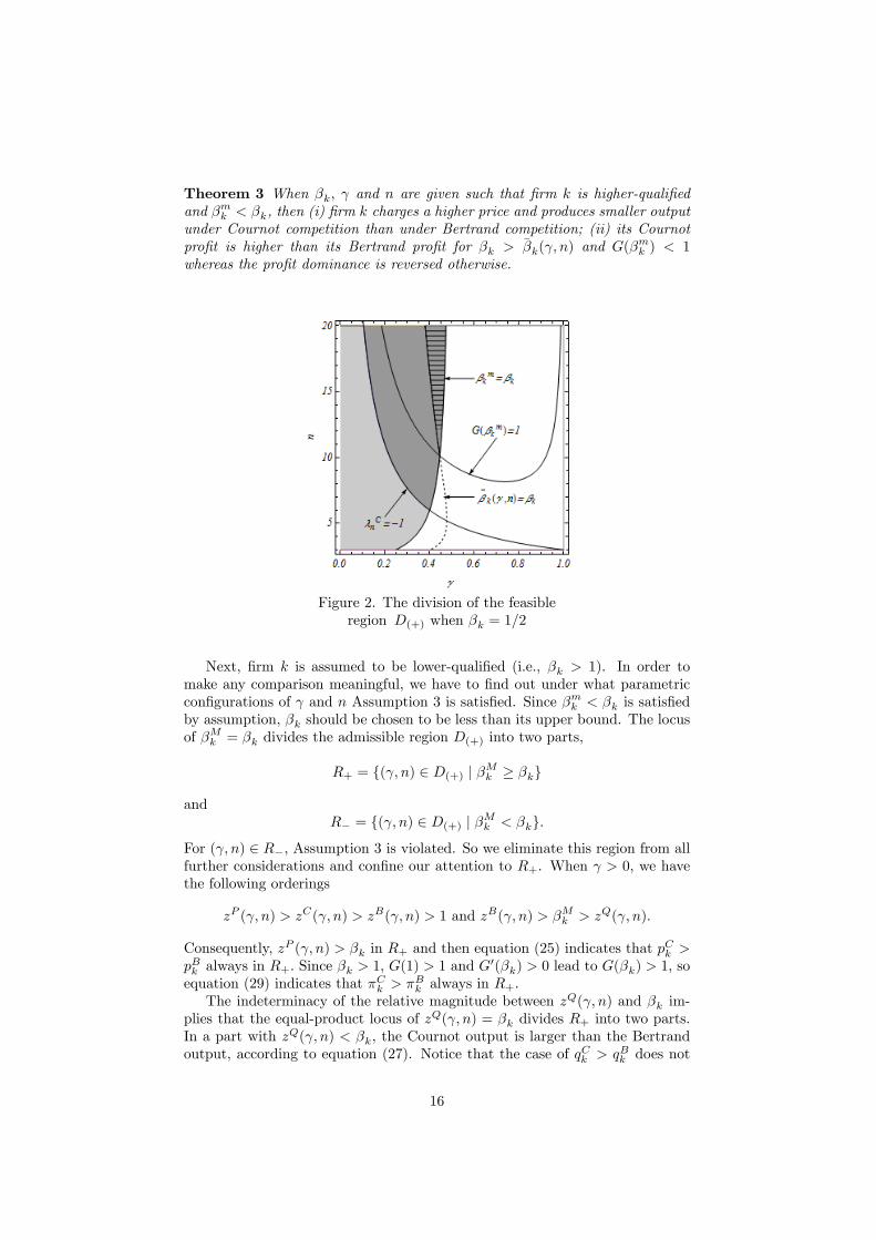
Theorem 3 When �k; and n are given such that �rm k is higher-quali�edand �mk < �k, then (i) �rm k charges a higher price and produces smaller outputunder Cournot competition than under Bertrand competition; (ii) its Cournotpro�t is higher than its Bertrand pro�t for �k > ��k( ; n) and G(�

mk ) < 1

whereas the pro�t dominance is reversed otherwise.

Figure 2. The division of the feasibleregion D(+) when �k = 1=2

Next, �rm k is assumed to be lower-quali�ed (i.e., �k > 1). In order tomake any comparison meaningful, we have to �nd out under what parametriccon�gurations of and n Assumption 3 is satis�ed. Since �mk < �k is satis�edby assumption, �k should be chosen to be less than its upper bound. The locusof �Mk = �k divides the admissible region D(+) into two parts,

R+ = f( ; n) 2 D(+) j �Mk � �kg

andR� = f( ; n) 2 D(+) j �Mk < �kg:

For ( ; n) 2 R�; Assumption 3 is violated. So we eliminate this region from allfurther considerations and con�ne our attention to R+. When > 0; we havethe following orderings

zP ( ; n) > zC( ; n) > zB( ; n) > 1 and zB( ; n) > �Mk > zQ( ; n):

Consequently, zP ( ; n) > �k in R+ and then equation (25) indicates that pCk >

pBk always in R+: Since �k > 1; G(1) > 1 and G0(�k) > 0 lead to G(�k) > 1; so

equation (29) indicates that �Ck > �Bk always in R+:

The indeterminacy of the relative magnitude between zQ( ; n) and �k im-plies that the equal-product locus of zQ( ; n) = �k divides R+ into two parts.In a part with zQ( ; n) < �k; the Cournot output is larger than the Bertrandoutput, according to equation (27). Notice that the case of qCk > q

Bk does not

16

emerge in duopolies and its possibility is not examined in Häckner (2000). The�Mk = �k locus crosses the �

Cn = �1 locus at point (� ; �n) with

� =3

�k� 2 and �n = 1 + 2

� :

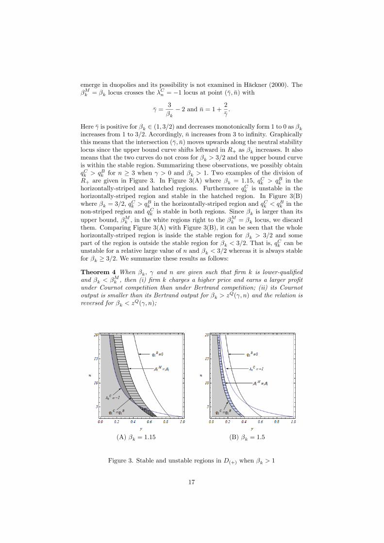
Here � is positive for �k 2 (1; 3=2) and decreases monotonically form 1 to 0 as �kincreases from 1 to 3=2: Accordingly, �n increases from 3 to in�nity. Graphicallythis means that the intersection (� ; �n) moves upwards along the neutral stabilitylocus since the upper bound curve shifts leftward in R+ as �k increases. It alsomeans that the two curves do not cross for �k > 3=2 and the upper bound curveis within the stable region: Summarizing these observations, we possibly obtainqCk > qBk for n � 3 when > 0 and �k > 1: Two examples of the division ofR+ are given in Figure 3. In Figure 3(A) where �k = 1:15, qCk > qBk in thehorizontally-striped and hatched regions. Furthermore qCk is unstable in thehorizontally-striped region and stable in the hatched region. In Figure 3(B)where �k = 3=2; q

Ck > q

Bk in the horizontally-striped region and q

Ck < q

Bk in the

non-striped region and qCk is stable in both regions. Since �k is larger than itsupper bound, �Mk ; in the white regions right to the �

Mk = �k locus, we discard

them. Comparing Figure 3(A) with Figure 3(B), it can be seen that the wholehorizontally-striped region is inside the stable region for �k > 3=2 and somepart of the region is outside the stable region for �k < 3=2: That is, q

Ck can be

unstable for a relative large value of n and �k < 3=2 whereas it is always stablefor �k � 3=2: We summarize these results as follows:

Theorem 4 When �k; and n are given such that �rm k is lower-quali�edand �k < �

Mk , then (i) �rm k charges a higher price and earns a larger pro�t

under Cournot competition than under Bertrand competition; (ii) its Cournotoutput is smaller than its Bertrand output for �k > z

Q( ; n) and the relation isreversed for �k < z

Q( ; n);

(A) �k = 1:15 (B) �k = 1:5

Figure 3. Stable and unstable regions in D(+) when �k > 1

17

3.3 The goods are complements, < 0

When < 0; equation (28) implies qCk < qBk always as zQ( ; n) < 0 for any

and n in DB regardless of whether �k is greater or less than unity. It shouldbe noticed that the non-induced demand is always positive and Assumption 3is not necessary. However, the lower bound of �k is de�ned to be 1=n when thenet qualities of any other �rms are zero.The pro�t ratio for �k = 1=n is reduced to

G

�1

n

�= A( ; n)2B( ; n)

�(1 + (n� 2) )(2 + (n� 2) )

2 + 3(n� 2) + (n2 � 5n+ 5) 2

�2:

Although it is indeterminate in general whether G(1=n) is greater or less thanunity,5 it can be shown that

G

�1

n

�< 1 for 2 ( 0; 0) when n = 8

and

G

�1

n

�> 1 for 2 ( 1; 2) when n = 9

where 0 = 1=(n � 1); i 2 ( 0; 0) for i = 1; 2 are the solutions of equationG(1=n) = 1:Hence there is a threshold value �n 2 (8; 9) of n such thatG(1=�n) = 1has a unique solution � 2 ( 0; 0). It is numerically obtained that � ' �0:133and �n = 8:16: Since it is indeterminate whether G(1=n) is greater or less thanunity, the G(1=n) = 1 locus divides the region DB into two parts, one withG(1=n) < 1 and the other with G(1=n) > 1; which is above the n = �n line.If n < nk, then �

mk (= 1=n) > �k: This inequality violates the assumption

that the net quality �k is greater or equal to its lower bound, �mk : Thus this

case is eliminated from considerations. Having n � nk; we should still distinguishbetween the following three cases,

nk < n � �n; nk � �n � n and �n < nk < n:

We start with the �rst case, nk < n � �n. Condition n � �n and G0 < 0 implythat G(1=n) � G(1=�n) for 2 ( 0; 0). It has been shown that G(1=�n) � 1 for 2 ( 0; 0): �k � 1=n (= �mk ) implies that G(�k) � G(1=n) � 1. Hence our �rstresult on the pro�t di¤erence is that

�Ck � �Bk if nk < n � �n:

Returning to the de�nitions of ~�k and �n; we have

~�k(� ; �n) =1

�n:

We denote this threshold value of �k by �� = ~�k(� ; �n) or �� = 1=�n: Simplecalculation shows that �� ' 0:123: In Figure 4 below, the graphs of ~�( ; n)with changing values of n are depicted against : The left most graph is for

5 It is shown that lim �>0

G(1=n) = 1 and lim �>1=(1�n)

G(1=n) = 0:

18

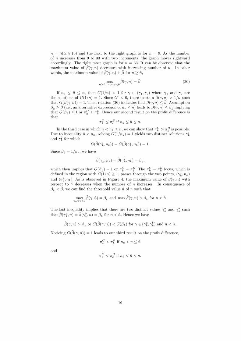
n = �n(' 8:16) and the next to the right graph is for n = 9: As the numberof n increases from 9 to 33 with two increments, the graph moves rightwardaccordingly. The right most graph is for n = 33: It can be observed that themaximum value of ~�( ; n) decreases with increasing number of n. In otherwords, the maximum value of ~�( ; n) is �� for n � �n;

maxn��n; 0< <0

~�( ; n) = ��: (36)

If nk � �n � n, then G(1=n) > 1 for 2 ( 1; 2) where 1 and 2 arethe solutions of G(1=n) = 1: Since G0 < 0, there exists a ~�( ; n) > 1=n suchthat G(~�( ; n)) = 1: Then relation (36) indicates that ~�( ; n) � ��: Assumption�k � �� (i.e., an alternative expression of nk � �n) leads to ~�( ; n) � �k implyingthat G(�k) � 1 or �Ck � �Bk : Hence our second result on the pro�t di¤erence isthat

�Ck � �Bk if nk � �n � n:

In the third case in which �n < nk � n; we can show that �Ck > �Bk is possible.Due to inequality �n < nk; solving G(1=nk) = 1 yields two distinct solutions 1kand 2k for which

G(~�( 1k; nk)) = G(~�( 2k; nk)) = 1:

Since �k = 1=nk; we have

~�( 1k; nk) =~�( 2k; nk) = �k;

which then implies that G(�k) = 1 or �Ck = �

Bk : The �

Ck = �

Bk locus, which is

de�ned in the region with G(1=n) � 1; passes through the two points, ( 1k; nk)and ( 2k; nk): As is observed in Figure 4, the maximum value of ~�( ; n) withrespect to decreases when the number of n increases. In consequence of�k <

��; we can �nd the threshold value n̂ of n such that

max 0< <0

~�( ; n̂) = �k and max ~�( ; n) > �k for n < n̂:

The last inequality implies that there are two distinct values ak and bk such

that ~�( ak; n) = ~�( bk; n) = �k for n < n̂: Hence we have

~�( ; n) > �k or G(~�( ; n)) < G(�k) for 2 ( ak; bk) and n < n̂:

Noticing G(~�( ; n)) = 1 leads to our third result on the pro�t di¤erence,

�Ck > �Bk if nk < n � n̂

and�Ck < �

Bk if nk < n̂ < n:

19

Figure 4. Various ~�( ; n) curves aginst ;given n

It is worthwhile to point out that a higher-quali�ed �rm k possibly earnsmore pro�ts under Cournot competition if its net quality di¤erence is large tothe extent that �k < ��k( ; n). In the case when the goods are complements,the dominance of Cournot pro�t over Bertrand pro�t is not observed in Singhand Vives (1984) and Häckner (2000). Figure 5 is an enlargement of the secondquadrant of Figure 1 and represents the division of the feasible region DB when�k = 0:1 (i.e., nk = 10): Notice �rst that the white region is a union of theregion with 1+ (n� 1) < 0 and the region with n < nk and thus is eliminatedfrom further considerations. The least dark-gray region is illustrated inside theunstable darker-gray region and is surrounded by the loci of G(1=n) = 1 andn = nk. Clearly G(1=n) > 1 holds inside. The equal-pro�t locus of ��k( ; n) =�k de�ned for n � nk divides the least dark-gray region into two parts andcrosses the G(1=n) locus at points ( 1k; nk) and (

2k; nk).

6 Cournot pro�t islarger than Bertrand pro�t in the horizontally-striped region surrounded by theequal-pro�t locus and the n = nk line while Bertrand pro�t is larger in the non-striped region. Needless to say, Bertrand pro�t is larger in any other regions

6Solving G(1=n) = 1 and �Ck = �Bk simultaneously yields nk = 10, 1k ' �0:11 and 2k ' �0:098:

20

with G(1=n) < 1.

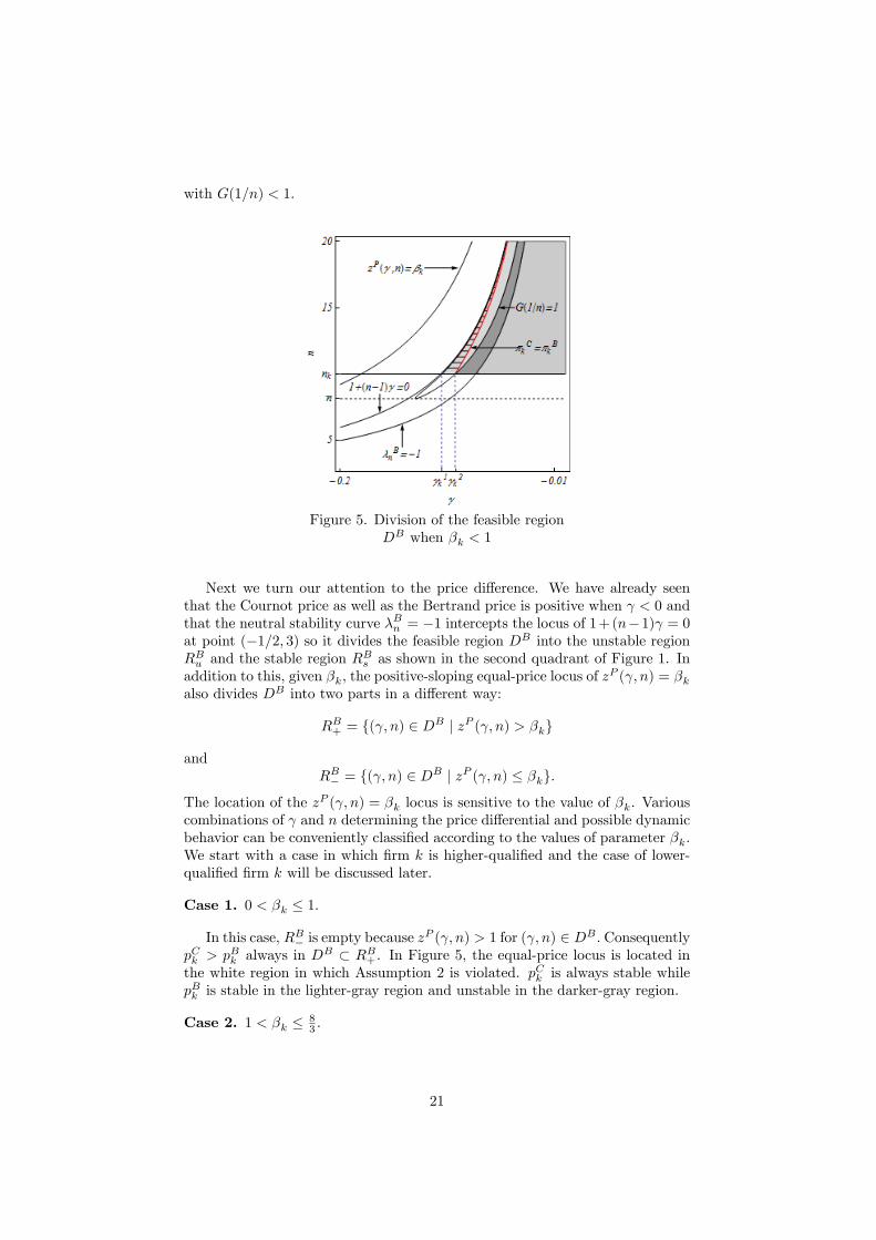
Figure 5. Division of the feasible regionDB when �k < 1

Next we turn our attention to the price di¤erence. We have already seenthat the Cournot price as well as the Bertrand price is positive when < 0 andthat the neutral stability curve �Bn = �1 intercepts the locus of 1+(n�1) = 0at point (�1=2; 3) so it divides the feasible region DB into the unstable regionRBu and the stable region R

Bs as shown in the second quadrant of Figure 1. In

addition to this, given �k; the positive-sloping equal-price locus of zP ( ; n) = �k

also divides DB into two parts in a di¤erent way:

RB+ = f( ; n) 2 DB j zP ( ; n) > �kg

andRB� = f( ; n) 2 DB j zP ( ; n) � �kg:

The location of the zP ( ; n) = �k locus is sensitive to the value of �k. Variouscombinations of and n determining the price di¤erential and possible dynamicbehavior can be conveniently classi�ed according to the values of parameter �k.We start with a case in which �rm k is higher-quali�ed and the case of lower-quali�ed �rm k will be discussed later.

Case 1. 0 < �k � 1:

In this case, RB� is empty because zP ( ; n) > 1 for ( ; n) 2 DB : Consequently

pCk > pBk always in DB � RB+. In Figure 5, the equal-price locus is located in

the white region in which Assumption 2 is violated. pCk is always stable whilepBk is stable in the lighter-gray region and unstable in the darker-gray region.

Case 2. 1 < �k � 83 :

21

When �k becomes greater than unity, the equal-price locus shifts downwardsand crosses the locus of 1 + (n� 1) = 0 at the point ( 1; n1) with

1 =1�

p1� � + �2

�and n1 = 1�

1

1:

The equal-price locus divides the unstable region RBu into two parts. In Figure6 where �k = 2;

7 RBu \RB� is located above the equal-price locus and vertically-striped, RBu \RB+ is bounded by the equal-price locus and the neutral stabilitylocus and RBs \RB+ is the lighter-gray region. The intersection moves downwardsalong the locus of 1+(n� 1) = 0 as �k increases from unity and arrives at thepoint (�1=2; 3) when �k = 8=3: Hence we have the following results concerningthe price di¤erence and the stability of the Bertrand price:

(2-i) pCk < pBk and p

Bk is unstable for ( ; n) 2 RBu \RB�;

(2-ii) pCk > pBk and p

Bk is unstable for ( ; n) 2 RBu \RB+;

(2-iii) pCk > pBk and p

Bk is stable for ( ; n) 2 RBs \RB+:

Figure 6, Division of DB when1 < �k <

83

Case 3. 83 < �k � 4:

When �k increases further from 8=3; then the equal-price locus interceptsthe neutral stability locus of �Bn = �1 from below at point ( 2; n2) with

2 =2(� � 4)5� � 8 and n2 =

5

3� 2

3 2:

7 In Figure 5, we take n = 8 and limit the interval of to (�0:5;�0:1) only for the sake ofgraphical convenience. Changing the values of n and enlarging the interval do not a¤ect thequalitative aspects of the results.

22

As shown in Figure 7 where �k = 3; the equal-price locus divides the unstableregion RBu into the vertically-striped gray region above the locus and the darker-gray region below. It also divides the stable region RBs into two parts: thehatched region above the locus and the light-gray region below. Since it is noteasy to see that the hatched region is bounded by the neutral stability locus andthe equal-price locus, the lower-left part of Figure 7 is enlarged and is insertedinto Figure 7. We have the following four possibilities concerning the pricedi¤erence and the stability of the Bertrand price in this case:

(3-i) pCk < pBk and p

Bk is unstable for ( ; n) 2 RBu \RB�;

(3-ii) pCk > pBk and p

Bk is unstable for ( ; n) 2 RBu \RB+;

(3-iii) pCk < pBk and p

Bk is stable for ( ; n) 2 RBs \RB�;

(3-iv) pCk > pBk and p

Bk is stable for ( ; n) 2 RBs \RB+:

Notice that � � can be de�ned for �k � 4: This implies that the intersectionmoves upward along the neutral stability locus as �k increases further up to 4:

Figure 7. Division of DB when83 < �k < 4

Case 4. �k > 4:

When �k becomes larger than 4; the equal-price locus is located below the�Bn = �1 locus. It then divides the stable region RBs into two parts, RBs \ RB�and RBs \ RB+: The former corresponds to the hatched region and the latterto the light-gray region in Figure 8 in which �k = 5. The hatched region thatappeared �rst in Figure 7 becomes larger with increasing value of �k. The wholeregion RBu is vertically striped, which means that the Bertrand price is largerthan the Cournot price and is unstable. We have therefore the following results

23

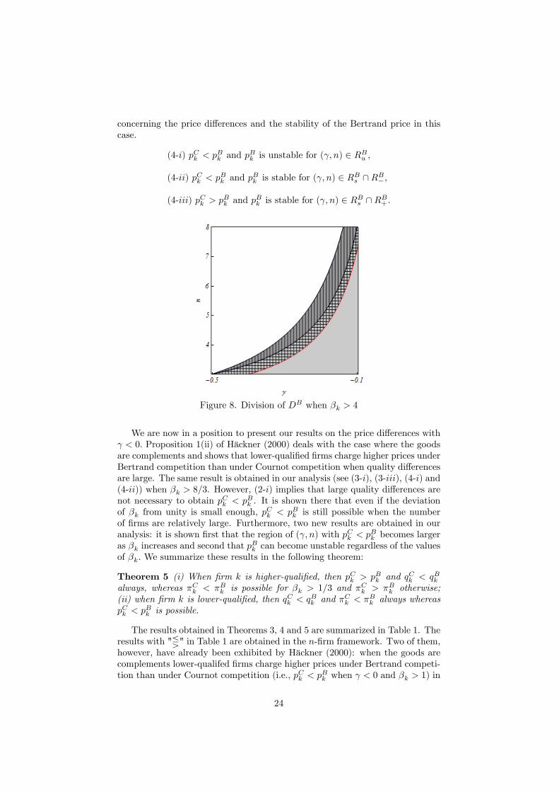
concerning the price di¤erences and the stability of the Bertrand price in thiscase.

(4-i) pCk < pBk and p

Bk is unstable for ( ; n) 2 RBu ;

(4-ii) pCk < pBk and p

Bk is stable for ( ; n) 2 RBs \RB�;

(4-iii) pCk > pBk and p

Bk is stable for ( ; n) 2 RBs \RB+:

Figure 8. Division of DB when �k > 4

We are now in a position to present our results on the price di¤erences with < 0. Proposition 1(ii) of Häckner (2000) deals with the case where the goodsare complements and shows that lower-quali�ed �rms charge higher prices underBertrand competition than under Cournot competition when quality di¤erencesare large. The same result is obtained in our analysis (see (3-i), (3-iii), (4-i) and(4-ii)) when �k > 8=3. However, (2-i) implies that large quality di¤erences arenot necessary to obtain pCk < p

Bk . It is shown there that even if the deviation

of �k from unity is small enough, pCk < pBk is still possible when the numberof �rms are relatively large. Furthermore, two new results are obtained in ouranalysis: it is shown �rst that the region of ( ; n) with pCk < p

Bk becomes larger

as �k increases and second that pBk can become unstable regardless of the values

of �k: We summarize these results in the following theorem:

Theorem 5 (i) When �rm k is higher-quali�ed, then pCk > pBk and qCk < qBkalways, whereas �Ck < �Bk is possible for �k > 1=3 and �Ck > �Bk otherwise;(ii) when �rm k is lower-quali�ed, then qCk < q

Bk and �Ck < �

Bk always whereas

pCk < pBk is possible.

The results obtained in Theorems 3, 4 and 5 are summarized in Table 1. Theresults with "Q" in Table 1 are obtained in the n-�rm framework. Two of them,however, have already been exhibited by Häckner (2000): when the goods arecomplements lower-qualifed �rms charge higher prices under Bertrand competi-tion than under Cournot competition (i.e., pCk < p

Bk when < 0 and �k > 1) in

24

his Proposition 1(ii) and when the goods are substitutes, higher-quali�ed �rmsearn higher pro�ts under Bertrand competition than under Cournot competi-tion (i.e., �Ck < �Bk when > 0 and �k < 1) in his Proposition 2(ii). We �rstcon�rm these results and then classify the parameter region into speci�ed sub-region in which these results hold as seen in Figures 2-8 except Figure 4. Inaddition, we demonstrate two new results: when the goods are complements,then higher-quali�ed �rms earn higher pro�ts under Cournot competition (i.e.,�Ck > �Bk when < 0 and �k < 1) and when the goods are substitutes, thenlower-quali�ed �rms may produce more output under Cournot competition (i.e.,qCk > q

Bk ).

Substitutes ( > 0) Complements ( < 0)

Higher-quali�ed(�k < 1)

pCk > pBk

qCk < qBk

�Ck Q �Bk

pCk > pBk

qCk < qBk

�Ck Q �Bk

Lower-quali�ed(�k > 1)

pCk > pBk

qCk Q qBk

�Ck > �Bk

pCk Q pBk

qCk < qBk

�Ck < �Bk

Table 1. Comparison of Cournot and Bertrand strategies

4 Concluding Remarks

Singh and Vives (1984) have shown that the duopoly model with linear demandand cost functions have de�nitive results concerning the nature of Cournot andBertrand competition as it was mentioned in the Introduction. Häckner (2000)increases the number of �rms to n from 2 and exhibits that some of these resultsare sensitive to the duopoly assumption. In this study, we examine the generaln-�rm oligopoly model and add two main �ndings to the existing literature onCournot and Bertrand competitions. The �rst �nding is concerned with thestability of Cournot and Bertrand equilibria. As stated in Theorems 1 and 2,Cournot equilibrium may be unstable whereas Bertrand equilibrium is alwaysstable when the goods are substitutes. It is further shown that Bertrand equi-librium may be unstable whereas Cournot equilibrium is always stable when thegoods are complements. This �nding extends the stability result of Theocharis(1960) that a Cournot oligopoly model is unstable if more than three �rms areinvolved and the goods are homogenous (i.e., perfectly substitutes).The second �nding is concerned with the comparison of Cournot and Bertrand

strategies. In addition to the inequality reversal of the price and quantity dif-ferences, the pro�t di¤erences shown in the duopoly framework may be re-versed in the n-�rm framework. Furthermore, as shown in Figures 2 and 5,

25

the horizontally-striped regions are located inside the instability regions. Thismeans that, for example, �Ck < �

Bk is possible when > 0 and �k < 1 however

�Ck is locally unstable. The result of �Ck < �Bk does not have much economicimplication from the dynamic point of view. Therefore the natural questionto be next raised should be concerned with the global dynamic properties ofthe locally unstable model. Matsumoto and Szidarovszky (2010) have alreadystarted their research in this direction.

References

[1] Gandolfo, G., Economic Dynamics (Study Edition), 2000,Berlin/Heidelberg/New York, Springer.

[2] Häckner, J. A Note on Price and Quantity Competition in Di¤erentiatedOligopolies, Journal of Economic Theory, 93 (2000), 233-239.

[3] Matsumoto, A., and F. Szidarovszky, Quantity and Price competition in aDynamic Di¤erentiated Oligopoly, Mimeo, (2010).

[4] Puu, T., Rational Expectations and the Cournot-Theocharis Problems, Dis-crete Dynamics in Nature and Society, 2006 (2006), 1-11.

[5] Singh, N. and X. Vives, Price and Quantity Competition in a Di¤erentiatedDuopoly, Rand Journal of Economics, 15 (1984), 546-554.

[6] Theocharis, R. D., On the Stability of the Cournot Solution on the OligopolyProblem, Review of Economic Studies, 27 (1960), 133-134.

26