Working Paper 4/2011

Price and welfare effects of

emission quota allocation Rolf Golombek, Sverre A.C. Kittelsen and Knut Einar Rosendahl

The CREE Centre acknowledges financial support from The Research Council of Norway, University of Oslo and user partners.

ISBN: 978-82-7988-105-6 ISSN: 1892-9680

http://cree.uio.no

1

Price and welfare effects of emission quota

allocation

Rolf Golombeka, Sverre A.C. Kittelsenb and Knut Einar Rosendahlc

Abstract:

We analyze how different ways of allocating emission quotas may influence the electricity market.

Using a large-scale numerical model of the Western European energy market, we show that different

allocation mechanisms can have very different effects on the electricity market, even if the total

emission target is fixed. This is particularly the case if output-based allocation (OBA) of quotas is

used. Gas power production is then substantially higher than if quotas are grandfathered or auctioned,

and the price of emissions is almost twice as high. Moreover, even though electricity prices are lower,

the welfare costs of attaining a fixed emission target are significantly higher. The paper analyzes other

allocation mechanisms as well, leading to yet more outcomes in the electricity market. The numerical

results for OBA are supported by theoretical analysis, with some new general results.

Keywords: Quota market; Electricity market; Allocation of quotas

JEL classification: D61; H23; Q41; Q58

Acknowledgement: We are grateful to Wenting Chen for valuable assistance, to Cathrine Hagem and

Ole Røgeberg for useful comments, and to the Renergi programme of the Research Council of Norway

(RCN) for financial support. While carrying out this research we have been associated with CREE -

Oslo Centre for Research on Environmentally friendly Energy. CREE is supported by the Research

Council of Norway.

a Frisch Centre. E-mail: rolf.golombek@frisch.uio.no b Frisch Centre. E-mail: sverre.kittelsen@frisch.uio.no c Corresponding author. Statistics Norway. E-mail: ker@ssb.no

2

1 Introduction

Emissions trading has become the most important policy instrument for regulating emissions to air,

with the EU Emissions Trading System (EU ETS) being the most prominent example so far.1 An

important element in any emission trading system (ETS) is how to allocate allowances, i.e., the rights

to emit.

Traditionally, economic analyses have focused on the comparison between auctioning and

(unconditional) grandfathering, pointing particularly to the following: First, both alternatives provide a

cost-effective outcome (Montgomery, 1972). Second, auctioning is generally preferred over

grandfathering from an economic welfare perspective due to auction revenues that can be used to

reduce distortionary taxes (Goulder, 1995). More recent literature has investigated the impacts of

alternative allocation mechanisms, not least because of the various allocation rules applied and

proposed in the EU ETS (see, e.g., Böhringer and Lange, 2005a,b; Fischer and Fox, 2007; Ellerman,

2008; Rosendahl, 2008; and Rosendahl and Storrøsten, 2011a). One main insight from this mainly

analytical literature is that the choice of allocation mechanism not only has distributional impacts, but

can also affect prices and quantities in the markets regulated by the ETS, and thus the cost-

effectiveness of the system.

In this paper we explore how various allocation mechanisms may play out in the electricity market,

using the European market as our context. Most of the literature on allocation mechanisms so far have

either had an analytical perspective (e.g., the cited references above), or used rather stylized numerical

models (see below for some exceptions). Our paper is, as far as we know, the most in-depth numerical

analysis of this issue so far. We find that the choice of allocation mechanism can indeed have

substantial impacts on electricity prices and market shares, even if the overall emission target is held

fixed. Moreover, the costs of complying with an emission target may increase substantially if certain

allocation mechanisms are chosen.

In particular, our numerical results suggest that allocating quotas in proportion to quantities

determined by the firms themselves, such as production or installed capacity, may induce large

changes in prices, market shares and welfare costs. This is especially true for output-based allocation

(OBA), for which allowances are distributed in proportion to each producer’s output, using so-called

1 http://ec.europa.eu/clima/policies/ets/index_en.htm

3

allocation factors.2 In this case we find that the welfare costs of complying with a certain emissions

target may increase by 70 percent relative to grandfathering (or full auctioning). This scenario is

characterized by a much higher price of emissions and a considerable increase in the market share of

gas power (relative to grandfathering).

The model we apply is an extensive numerical equilibrium model of the Western European energy

market (LIBEMOD, cf. Aune et al. 2008). The electricity market interacts in the model with the

markets of other energy goods, allowing us, for example, to calculate the welfare costs of different

scenarios. Electricity production and transmission between countries, including investments in new

production and transmission capacity, are modeled in detail, and electricity consumption is

endogenously determined by the price of electricity and other energy carriers. For the purpose of the

current study, the model has been extended to incorporate alternative allocation mechanisms. We

describe the model in more detail in Section 3.

In order to better understand the numerical findings with regards to OBA, we first use a simple

analytical model to show some general results about the effects of this allocation mechanism relative

to grandfathering. We first demonstrate that OBA generally leads to a higher price of emissions, a

result which is well known from earlier studies, e.g., Fischer (2001) and Fischer and Fox (2007). As

opposed to those two studies, we consider heterogeneous firms rather than a representative firm.

Higher emission price is clearly most detrimental to the most emission-intensive plants, and we show

that less emission-intensive plants will in general be better off under OBA. Moreover, we find that

more fuel efficient plants will benefit from OBA, but only if non-fuel costs are strictly convex. If non-

fuel costs are linear, however, output is unchanged if plants only differ with respect to fuel efficiency.

One interesting insight from the analytical part is that both demand for and supply of quotas are

declining in the price of quotas under OBA, given a fixed set of allocation parameters and the

government’s net sales of quotas (e.g., through auctioning): a higher emission price leads to lower

emissions (thus lower demand) and lower output (thus lower supply through OBA). This has bearings

2 Variants of OBA will be used in the next phase of the EU ETS (see Section 4 for details), and have also been included in

proposed cap-and-trade systems in the U.S. (e.g., House of Representatives, 2009). Whereas the EU ETS will allocate

quotas based on past output, most studies of OBA (including ours) assume that quotas are allocated based on current

output. OBA has previously been analyzed numerically in both electricity market models (see below) and CGE analysis

(Böhringer and Lange, 2005a; Fischer and Fox, 2007; Böhringer et al., 2010). Analytical studies (e.g., Fischer, 2001;

Böhringer and Lange, 2005b; Sterner and Muller, 2008; Rosendahl and Storrøsten, 2011b) have focused on e.g. price and

quantity effects, first- and second-best allocation mechanisms, and clean technology investments. The former study is the

most relevant here, and is further discussed below.

4

on the government’s supply-side policy in the quota market. If the government adjusts the OBA

allocation parameter, i.e., changes the number of allowances per unit output, then it must also adjust

either its net sales of quotas or the lump sum allocation of quotas to keep up with a fixed overall

emissions target. Hence, demand side policy must go along with a suitable supply side management.

We believe this point has not been adequately stressed in previous OBA studies.

Our paper relates to different strands of the literature, and we have already pointed to some related

analytical studies on the effects of OBA. As mentioned above, only a few numerical studies exist on

the relationship between allocation mechanisms and the electricity market. One such study is Neuhoff

et al. (2006). They use power dispatch models for the UK and the European electricity market, with

fixed demand for electricity, to examine how different allocation rules may affect CO2 emissions,

prices of CO2 and electricity, and the generation mix. Burtraw et al. (2006) investigate the impacts of

different allocation mechanisms in the Regional Greenhouse Gas Initiative (RGGI) among North

Eastern states in the U.S., using a simulation model of the electricity market in those states. Bode

(2006) simulates the effects of alternative allocation schemes using a power market model with five

different technologies and 110 power plants (located in a number of countries in different parts of the

world). These three studies cover some of the same issues as we focus on, but their models are not as

rich as the LIBEMOD model, e.g., with respect to inter-fuel competition, investments in different

types of capacity and welfare calculations. Their main findings with respect to prices and quantities

(e.g., under OBA) are largely consistent with the results we obtain.

Another strand of literature investigates the relationship between emissions trading on the one hand,

and electricity prices and quantities on the other, either from a general perspective or in the EU ETS

context. Yet, this literature has typically overlooked the effects of different allocation mechanisms. A

large part of this literature has examined to what degree CO2 prices are passed on to electricity prices..

Some studies have estimated the elasticity of the electricity price with respect to the CO2 price, finding

that this elasticity strongly depends on the generation mix in the market.3 Other studies have estimated

the marginal pass-through rate, i.e., the ratio of the increase in power price to the marginal generator’s

CO2 cost. For example, Lise et al. (2010), using a short-run simulation model covering the electricity

market of 20 European countries4, find that the marginal pass-through rate is 70-90 percent in most

countries and scenarios considered. Econometric studies find similar pass-through rates.5 In

3 For instance, Bunn and Fezzi (2007) for the UK, and Kirat and Ahamada (2011) for Germany and France.

4 See Chen et al. (2008) for an earlier version of the same model.

5 For instance, Sijm et al. (2006) for Germany and the Netherlands, Simshauser and Doan (2009) for Australia, and Fell

(2010) for the Nordic market.

5

comparison, our equilibrium pass-through rate (with unconditional allocation of quotas) is actually

slightly above 100 percent. This occurs because of higher gas prices due to increased gas demand.6

More importantly, with alternative allocation mechanisms, the pass-through rate tends to be lower,

substantially so (at around one third) under output-based allocation.

In the next section we derive some analytical results about the effects of output-based allocation. Then

in Section 3 we describe the numerical model LIBEMOD. Section 4 lays out the various policy

scenarios we consider and compare these with previous, current and upcoming allocation rules in the

EU ETS. Note that although our numerical analysis is performed in a European context, the allocation

mechanisms investigated are not a blueprint of the numerous allocation rules applied in the EU ETS.

Instead, our aim is to examine a few distinct and frequently used, or proposed, allocation mechanisms,

focusing on one alternative at a time. Section 5 presents the numerical results on how different

allocation mechanisms may affect the electricity market, and Section 6 concludes.

2 General effects of output-based allocation

2.1 Producer behaviour

In this section we use a theoretical model to study output-based allocation schemes. We consider a two

sector economy where in each sector s, 1, 2,s there is production of a homogenous good. Let isy be

production in firm i in sector s. Production requires use of fossil fuels x (measured in toe); let

( )is is isy y x be the production function of producer i in sector s, which is increasing and concave.

The input requirement function (inverse function of the production function), ( )is is isx x y , is then

increasing and convex, and shows how much fossil fuels isx that is required to produce isy .

Use of fossil fuels generates ( )is is isx y units of CO2 emissions where 0is is the emission

coefficient of firm i in sector s. Let s be the price of emissions in sector s. We assume that in sector

1 emissions are regulated through tradable quotas, whereas in sector 2 an emission tax 2 is imposed.

6 Which power producing technology is on the margin will vary across time and across countries (both in reality and in our

model). In general the demand for all fuels will change if electricity prices and/or CO2 prices change, and the equilibrium

effects in all markets simultaneously will determine the actual pass-through rates. The effect of changes in the markets for

natural gas tends to be the most important since the supply of natural gas is much less elastic than the supply of e.g. coal.

6

In sector 1 producer i is required to have 1 1 1( )i i ix y units of CO2 quotas in order to produce 1iy .

Further, for a moment we assume that in sector 1 producer i receives (free) quotas from one source

only, namely 0 01iy tradable quotas from the government. Here, 0 is a parameter (decided by the

government) and 01iy is a pre-determined variable, here production in firm i in sector 1 in an earlier

period. Hence, the net cost of purchasing quotas is 0 01 1 1 1 1( ( ) )i i i ix y y .

Finally, let sp be the output price in sector s, and let ( )is isc y be the costs of producing isy , which is

assumed to be increasing and convex, see discussion below. Note that ( )is isc y covers all costs

associated with producing isy except costs of emissions.

Producer i in sector 1 maximizes 0 01 1 1 1 1 1 1 1 1( ) ( ( ) )i i i i i i ip y c y x y y wrt. 1iy , which yields the

well-known first-order condition

1 1 1 1 1 1 1( ) ( ), .i i i i ip c y x y i (1) According to (1), at the margin the benefit of a marginal increase in production, 1,p should equal the

corresponding marginal cost, 1 1 1 1 1 1( ) ( )i i i i ic y x y , where the second term is the net marginal

emission cost of a unit of production. Note that 01iy is not contained in (1), which simply reflects that

this variable is predetermined. Hence, an increase in 0 will have no effect on the decision of the firm

– it will only imply a lump-sum transfer of money from the government to the firm.7

Assume, alternatively, that the firm receives quotas not only related to its past activity ( 01iy ), but also

related to its current activity such as current production, 1iy (output-based allocation). The number of

quotas received (in addition to 0 01iy ) is 1iy , where is a parameter decided by the government,

common to all firms in sector 1. In this case the firm maximizes

0 01 1 1 1 1 1 1 1 1 1( ) ( ( ) )i i i i i i i ip y c y x y y y wrt. 1iy , which yields the first-order condition

1 1 1 1 1 1 1( ) ( ( ) ), .i i i i ip c y x y i (2)

7 If producers think that future allocation may depend on current production, i.e., so-called updating (Rosendahl, 2008), the

first-order condition will change. This possibility is not considered in our analysis.

7

In (2) the firm takes into account that increased production will lead to increased costs

( 1 1 1 1 1 1( ) ( )i i i i ic y x y ) but also to more quotas received for free ( 1 ). Hence, the net marginal

emission cost is now “only” 1 1 1 1( ( ) ),i i ix y which is lower than in the previous case,

1 1 1 1( ),i i ix y see (1). In order to make the problem interesting and relevant, we assume

( ) 0x yi i i for all firms, that is, net marginal emission cost is positive. An increase in will

have impact on the decision of the firm; marginal emission costs will decrease, and hence the firm will

increase its production and emissions.

In the other sector, referred to as the tax sector ( 2s ), there is a tax 2 imposed on all emissions.

Each firm i maximizes 2 2 2 2 2 2 2 2( ) ( )i i i i i ip y c y x y , and the corresponding first-order condition is

2 2 2 2 2 2 2( ) ( ), ,i i i i ip c y x y i (3) which is equivalent to (1).

Above we have discussed the decisions of a firm. Clearly, changes at the firm level have market

implications; if firms receive quotas according to their level of production ( 1iy ), and increases,

the price of quotas may change. This will lead firms to adjust inputs and outputs. Therefore, we now

consider equilibrium effects of shifts in output-base allocation rules.

2.2 Market equilibrium

Below we distinguish between two policy cases; Case A where emissions in each sector are fixed (and

the price of emissions typically differs across sectors), and Case B where the price of emission is the

same in the two sectors. In both cases, total emissions in the economy are fixed.

In each sector, firms produce a homogenous good and the price of the good depends on total

production of the good represented by the inverse demand function for good s:

( ) 0.s s is si

p p y p (4)

The first-order condition for firms is given by relations (2) and (3), which for given levels of ,s sp

determines the supply of the goods isy . Further, total demand for emissions in each sector is given by

8

( ),s is is isi

D x y (5)

which are functions of ,s sp through isy .

In the quota sector, demand for quotas equals the demand for emissions, while the total supply of

quotas is:

0 01 1 1( )i i

i

T y y g (6)

where 0 01 1( )i i

i

y y are quotas received by firms and g is net sales of quotas from the

government. Thus 1T is also a function of 1 1,p . Equilibrium in the quota market is given by:

1 1D T (7) Actual emissions in each sector, se , must equal total demand for emissions:

.s se D (8) Finally, total emissions in the economy, E, equal the sum of emissions in each sector:

1 2.E e e (9)

Case A: Fixed sectoral emissions

Below we will always treat E as an exogenous variable. With fixed sectoral emissions, both 1e and 2e

are de facto exogenous variables, but formally one of them will be determined from relation (9), and

hence endogenous. Below we let 2e be endogenous.

Relations (2) - (9) determine the variables 01, , , , ,is s s sy p D T and 2e , given the exogenous

variables , ,g E and 1 .e Note that g may take “any” value (provided there is a corresponding

equilibrium), for example, zero. Furthermore, we may alternatively let g or be an endogenous

variable and 0 an exogenous variable. Also note that there is no interaction between the two sectors:

Relations (2), (4) (for 1s ), (5) (for 1s ), (6), (7) and (8) (for 1s ) determine 1 1 1 1 1, , , ,iy p D T

and 0 given the exogenous variables , g and 1 ,e and relations (3), (4) (for 2s ), (5) (for

9

2s ),Error! Reference source not found.(8) (for 2s ) Error! Reference source not found. and

(9) determine 2 2 2 2, , ,iy p D and 2e for given E. Hence, a change in will have no impact on the tax

sector.

Case B: A common price of emissions

Now there is a common price of emissions, that is,

1 2 . (10) Because of (10) the two sectors are now interlinked. The fourteen relations (2) - (10) determine the

variables 1, , , , , ,is s s s sy p D T e and 0 , given the exogenous variables , g and E.

2.3 Equilibrium effects of changes in the allocation parameter

We now examine how a change in , i.e., the output-based allocation parameter, affects the

equilibrium. We start with the case of fixed sectoral emissions, and then examine the case of a

common price of emissions.

Case A: Fixed sectoral emissions

From relations (2) and (4) we have

1 11( , ).i iy y (11)

Differentiation of (2) with respect to , using (11), gives

1 0.iy

Moreover, by differentiating (2)

with respect to 1 and using (11), we can derive an expression for

1

1

iy

. Typically,

1

1

iy

is negative,

but if production units are “sufficiently different”, this partial derivative may be positive for some

units. For example, units with a very low emission coefficient ( ), and/or firms requiring only a small

10

increase in the use of fossil fuels for a given increase in production ( ( )x y ), are candidates for a

positive derivate.8 Below we assume that

1

1

0,iy

for all firms.

Inserting (11) into (5) and (6), and differentiating with respect to 1 , we find how aggregate demand

for quotas, and aggregate supply of quotas, depend on the price of quotas. Because

1

1

0,iy

both

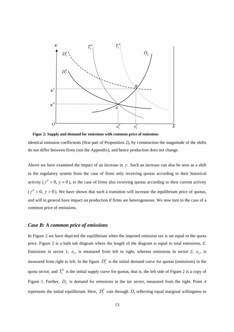
demand for, and supply of, quotas are decreasing in the price of quotas. In Figure 1 we have depicted

demand for, and supply of, quotas (for given values of g, γ0 and γ). In the figure the demand curve cuts

through the supply curve from below. This requires that

1 11 1

1 1

i ii i

y yx

, that is,

1

1 11

( ) 0ii i

yx

, which is fulfilled under our assumption, reflecting that net marginal cost of

emissions is positive ( ( ) 0x yi i i ).

8 With two firms in sector 1, here termed 1 and 2, then for firm 1 the derivative of production wrt. the quota price

partly depends on the term 11 11 11 21 21 21 1( ( ) ( )) ,x y x y p whereas the corresponding term for firm 2 is

21 21 21 11 11 11 1( ( ) ( )) .x y x y p We see that for firm 1 the term will be positive if 11 11 11 21 21 21( ) ( ),x y x y and

could possibly dominate the negative terms in the expression for 111 /y .

A

01D

11D

01T 2

1T

B

11T

O

1

1e 1e

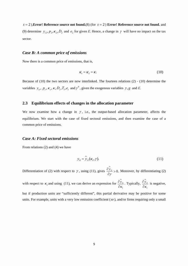
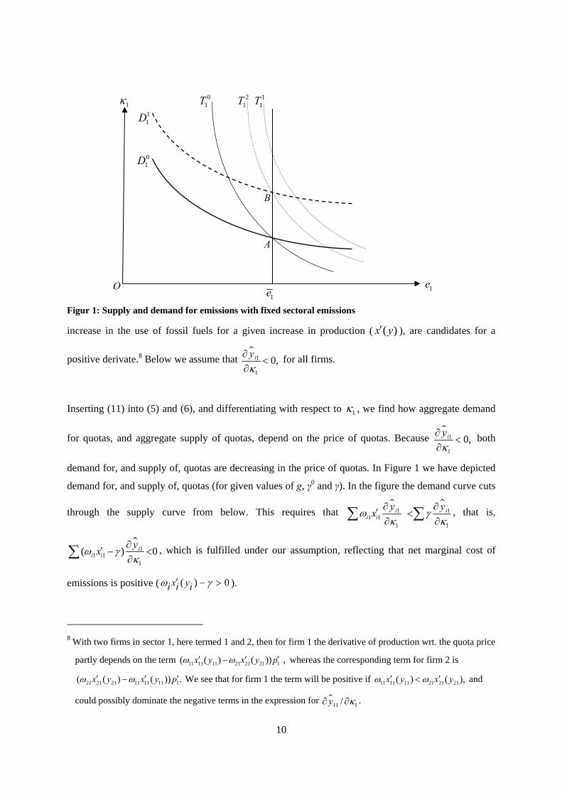
Figur 1: Supply and demand for emissions with fixed sectoral emissions

11

In Figure 1, 01D is the initial demand curve for quotas (emissions), 0

1T is the initial supply curve of

quotas, and A is the initial equilibrium. Assume now that increases. Under our assumptions, both

demand for quotas and supply of quotas will shift upwards (

1 0iy

). The shift in aggregate demand

(from 01D to 1

1D ), together with the assumption of a fixed level of emissions 1,e determine the new

equilibrium B, see Figure 1. As seen from the figure, the price of quotas 1 has increased.

We now examine in more detail how the equilibrium changes due to a shift in . First, the demand

curve shifts by

11 1 ,i

i i

yx

whereas the supply curve shifts by

1

1( )ii

yy

(In Figure 1, 1

1T is

the supply curve after the shift in ). Under our assumptions we do not know whether the shift

(measured vertically) is larger for demand than for supply. In Figure 1 we have assumed that the shift

in demand is smallest, which is consistent with the numerical cases in Section 5. Then the government

has to decrease 0 by so much that the new supply curve ( 21T in Figure 1) goes through B.

So far we have assumed that the government’s sale of quotas is given. Assume the opposite, that is,

the government sells or buys quotas as a response to market changes, and keeps γ0 fixed. Then g is an

endogenous variable, and both 0 and are exogenous. If now increases, then again 01D shifts to

11D , and hence B still represents the new equilibrium. Thus, all prices and quantities are identical

between these two cases. However, the government now has to adjust g such that 21T goes through B.

Hence, in Figure 1 g is decreased (instead of 0 ). From (6) we know that the change in g, when γ0 is

held fixed, has to equal the change in 0 01iy , if g had been held fixed.

The discussion above can be summarized as follows:

Proposition 1: If sectoral emissions are given, and firms in the quota sector receive more quotas for

each unit of production ( increases), the price of emissions increases. To reach the new equilibrium

the government has to either change the number of free quotas related to firms’ emissions in an

earlier period (adjust 0 ), or change its net sale of quotas (adjust g).

As mentioned in the introduction, the first part of Proposition 1 has been shown in previous studies

such as Fischer (2001) and Fischer and Fox (2007). Note, however, that we assume heterogeneous

12

firms, each with a concave production function. This is in contrast to the two above-mentioned studies,

which assumed homogenous firms (modelled as a representative firm), whose unit costs are decreasing

in their emissions rate but otherwise constant.

If firms are identical, an increase in will not change emissions at the firm level simply because total

emissions are given in the quota sector. Hence, also production at the firm level does not change, and

therefore the output price (in the quota sector) is unaltered.

With heterogeneous firms, an increase in will affect emissions and production at the firm level, and

therefore also market shares will change. It seems reasonable to presume that firms that are fossil-fuel

intensive, or firms with a high emission coefficient, will, cet. par., decrease their market shares,

reflecting that these firms will suffer the most from a higher price of quotas (which is caused by the

increase in ). In Appendix A we show that in general these conjectures are correct. We assume that

costs of production consist of two terms, fuel costs and non-fuel costs (the latter is identical across

firms), and prove the following propositions:

Proposition 2: Suppose that sectoral emissions are given and that there are two types of firms in the

quota sector; type 1 is more fossil-fuel intensive than type 2. Assume that firms receive more quotas

for each unit of production ( increases). If non-fuel costs are linear, then production in each firm

does not change. If non-fuel costs are strictly convex, then production in type 1 (2) firm decreases

(increases) and total production increases.

Proposition 3: Suppose that sectoral emissions are given and that there are two types of firms that

differ only with respect to the emission coefficient. If firms receive more quotas for each unit of

production ( increases), then production in firms with the lowest (highest) emission coefficient

increases (decreases), and total production increases.

The intuition behind Propositions 2 and 3 is straight forward. If firms receive more quotas for each

unit of production, then demand for quotas increases and total production tends to increase. Because

total emissions in the sector are fixed, the price of quotas increases. All firms are hurt by the raise in

the quota price, but firms that are fossil-fuel intensive, or have high emission coefficient, are hurt the

most. In these firms production decreases. For the other type of firm, the initial effect of a lower ,

which decreases marginal cost of production, dominates the (generated) effect of a higher quota price,

that is, in these firms production increases. Finally, in the special case of linear non-fuel costs and

13

identical emission coefficients (first part of Proposition 2), by construction the magnitude of the shifts

do not differ between firms (see the Appendix), and hence production does not change.

Above we have examined the impact of an increase in . Such an increase can also be seen as a shift

in the regulatory system from the case of firms only receiving quotas according to their historical

activity ( 0 0, 0 ), to the case of firms also receiving quotas according to their current activity

( 0 0, 0 ). We have shown that such a transition will increase the equilibrium price of quotas,

and will in general have impact on production if firms are heterogeneous. We now turn to the case of a

common price of emissions.

Case B: A common price of emissions

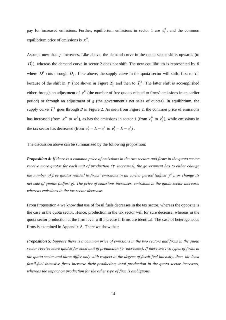
In Figure 2 we have depicted the equilibrium when the imposed emission tax is set equal to the quota

price. Figure 2 is a bath tub diagram where the length of the diagram is equal to total emissions, E.

Emissions in sector 1, 1e , is measured from left to right, whereas emissions in sector 2, 2e , is

measured from right to left. In the figure 01D is the initial demand curve for quotas (emissions) in the

quota sector, and 01T is the initial supply curve for quotas, that is, the left side of Figure 2 is a copy of

Figure 1. Further, 2D is demand for emissions in the tax sector, measured from the right. Point A

represents the initial equilibrium. Here, 01D cuts through 2D reflecting equal marginal willingness to

A

01D

11D

01T

21T

B

2D

O

01e 1

1e E

1

0

Figur 2: Supply and demand for emissions with common price of emissions

14

pay for increased emissions. Further, equilibrium emissions in sector 1 are 01e , and the common

equilibrium price of emissions is 0.

Assume now that increases. Like above, the demand curve in the quota sector shifts upwards (to

11D ), whereas the demand curve in sector 2 does not shift. The new equilibrium is represented by B

where 11D cuts through 2D . Like above, the supply curve in the quota sector will shift; first to 1

1T

because of the shift in (not shown in Figure 2), and then to 21T . The latter shift is accomplished

either through an adjustment of 0 (the number of free quotas related to firms’ emissions in an earlier

period) or through an adjustment of g (the government’s net sales of quotas). In equilibrium, the

supply curve 21T goes through B in Figure 2. As seen from Figure 2, the common price of emissions

has increased (from 0 to 1 ), as has the emissions in sector 1 (from 01e to 1

1e ), while emissions in

the tax sector has decreased (from 0 02 1e E e to 1 1

2 1e E e ) .

The discussion above can be summarized by the following proposition:

Proposition 4: If there is a common price of emissions in the two sectors and firms in the quota sector

receive more quotas for each unit of production ( increases), the government has to either change

the number of free quotas related to firms’ emissions in an earlier period (adjust 0 ), or change its

net sale of quotas (adjust g). The price of emissions increases, emissions in the quota sector increase,

whereas emissions in the tax sector decrease.

From Proposition 4 we know that use of fossil fuels decreases in the tax sector, whereas the opposite is

the case in the quota sector. Hence, production in the tax sector will for sure decrease, whereas in the

quota sector production at the firm level will increase if firms are identical. The case of heterogeneous

firms is examined in Appendix A. There we show that:

Proposition 5: Suppose there is a common price of emissions in the two sectors and firms in the quota

sector receive more quotas for each unit of production ( increases). If there are two types of firms in

the quota sector and these differ only with respect to the degree of fossil-fuel intensity, then the least

fossil-fuel intensive firms increase their production, total production in the quota sector increases,

whereas the impact on production for the other type of firm is ambiguous.

15

Proposition 6: Suppose there is a common price of emissions in the two sectors and firms in the quota

sector receive more quotas for each unit of production ( increases). If there are two types of firms in

the quota sector and these differ only with respect to the emission coefficient, then firms with the

lowest emission coefficient increase their production, total production in the quota sector increases,

whereas the impact on production for the other type of firm is ambiguous.

The results in Propositions 5 and 6 are quite similar to those in Propositions 2 and 3. The exception is

the impact on firms being fossil-fuel intensive or having a high emission coefficient. In Propositions 2

and 3, production in these firms decreases (or is unchanged in a special case), whereas in Propositions

5 and 6 the effect is ambiguous. The difference reflects that in the latter case emissions decrease in

sector 2, thereby opening up for increased emissions in sector 1 because total emissions are fixed.

3 Description of the numerical model LIBEMOD

LIBEMOD is a numerical multi-market equilibrium model for the energy sector. Its main focus is on

the electricity and natural gas industry in Western Europe, but it also covers markets for other fuels

like coal and oil. The model is a synthesis of the bottom up and top-down modeling traditions. On the

one hand it offers a detailed description of the electricity and natural gas industry in Western Europe,

in particular production of electricity, and on the other hand it has a clear foundation in economic

theory by deriving structural behavioral relations from well-specified optimization problems, and

imposing that all markets should clear.

LIBEMOD is well suited to analyze the impact of different allocation mechanisms for CO2 quotas

because the model has a rich description of costs in electricity production. In the model, the responses

of profit-maximizing electricity producers to allocation mechanisms have impacts on production and

investment of electricity, and might also differ between electricity technologies, for example between

coal-fired plants, gas-fired plants and renewables. LIBEMOD determines all energy quantities and all

energy prices, and CO2 prices are also determined within the model.

We now give a more detailed description of the model; see Aune et al. (2008) for a complete

description of the model, including detailed documentation of data sources and calibration strategy.

LIBEMOD distinguishes between model countries and other countries. In a model country, there is

production, investment, trade and consumption of all energy goods, that is, electricity, natural gas,

three types of coal (coking coal, steam coal and lignite), oil, and biomass. In LIBEMOD, each of

sixteen countries in Western Europe (Austria, Belgium, Denmark, Finland, France, Germany, Greece,

Ireland, Italy, the Netherlands, Norway, Spain, Sweden, Switzerland, Portugal and the United

16

Kingdom) is a model country, whereas all other countries in the world are represented mainly through

supply of, and demand for, coal and oil.

Electricity and natural gas are traded in competitive well-integrated Western European markets, using

existing capacity in international transmission of these energy goods. These capacities will be

expanded (in the model) if there are profitable investment opportunities. Coking coal, steam coal and

oil are traded in competitive global markets, whereas lignite (used for emission-intensive coal-power

production) and biomass (used to produce electricity) is traded in national markets only.

There are four groups of users of energy in each model country. First, there is intermediate demand

from electricity producers: for example, gas power producers demand natural gas. Furthermore, there

is demand from end users: the household, industry and transport sectors, though the latter demands

only oil products. For end users, demand is derived from a nested CES utility function with five levels.

At the top-nest level, there are substitution possibilities between energy-related goods and other forms

of consumption. At the second level, consumers face a trade-off between consumption based on the

different energy sources. Each of these is a nest describing complementarity between the actual energy

source and consumption goods that use this energy source (for example, electricity and electrical

appliances). Finally, the fourth and fifth levels are specific to electricity in defining the substitution

possibilities between summer and winter (season) and between day and night. Thus, except for

electricity, energy goods are traded in annual markets. Note that the calibrated parameters of the utility

functions differ between end users and countries.

In each model country, there is production of electricity by various technologies: steam coal power,

lignite power, gas power, oil power, reservoir hydro power, pumped storage power, nuclear power,

waste power and wind power. Some of these are not available in all countries. There are costs related

to electricity production: fuel costs, non-fuel operating costs, maintenance costs (related to the

maintained power capacity), start-up costs and investment costs. The power producer obtains revenues

either from using the maintained power capacity to produce and sell electricity, or by selling part of

the maintained power capacity to a national system operator who buys reserve power capacity in order

to ensure (if necessary) that the national electricity system does not break down.

Power producers face some technical constraints. For example, maintained capacity should not exceed

installed capacity. In addition, there are technology-specific constraints. For example, for reservoir

hydro, the reservoir filling at the end of a season cannot exceed the reservoir capacity, and total use of

water cannot exceed total availability of water (the sum of seasonal inflow of water and reservoir

filling at the end of the previous season). Each power producer maximizes profits subject to the

17

technical constraints. This optimization problem implies a number of first-order conditions, which

determine the operating and investment decisions of the producer.

LIBEMOD distinguishes between existing power plants - those that were available for production in

the data year 2000 - and new plants. For existing plants, the capacity is exogenously depreciated over

time and cannot be expanded. Moreover, for each type of fossil fuel based technology, and for each

model country, efficiency typically varies across existing plants. New plants are “built” in the model if

such investments are profitable. For new fossil fuel based technologies, efficiency does not differ

between the same type of plant, but differs across technologies.

LIBEMOD determines all energy quantities – investment, production, trade and consumption – all

energy prices, both producer prices and end-user prices, and also emission of CO2 by sector and

country. The model has been calibrated to the year 2000, imposing that the parameters should

reproduce observed demand, costs and efficiency distributions in 2000. For markets that we assume

were competitive in 2000, that is, the coal and crude oil markets, calibrated prices will be identical to

observed market prices. For other good, for example, natural gas and electricity, observed prices differ

from calibrated prices, reflecting market imperfections in 2000 whereas we impose competitive

markets in the calibration equilibrium.9

For the CES utility functions (one for each type of end-user in each model country), the parameters are

calibrated to minimize the deviation from exogenous own-price and cross-price demand elastiticies,

where the target values are based on literature estimates. For households, the own-price elasticities are

in the range of -0.4 to -0.6, while for industry the range runs from -0.5 to -0.7. For each model country

there is a load curve with four segments – one for each time period. According to our data, demand is

typically higher in winter than in summer (heating requires more energy than cooling), and higher

during the day than at night. For a more detailed description of LIBEMOD, including data sources, see

Aune et al. (2008).

4 Policy scenarios

In the numerical analysis we will examine the effects in the Western European energy market of

different allocation mechanisms. The four sectors in LIBEMOD are divided into two groups: The

electricity sector and the “rest-sector” (i.e., industry, household and transport sectors). For the former

9 The model is solved in USD2000 prices, but the model results are converted to Euro2010 using a PPP conversion rate and a

producer price index for the Euro area (http://stats.oecd.org/Index.aspx?DataSetCode=SNA_TABLE4)

18

sector we assume that all electricity producers in Western Europe are part of a common emission

trading system (ETS). For the rest-sector we assume that each country implements a CO2-tax, which is

either country-specific or equal across countries (more details below). We will consider the year 2010,

which is in the middle of the Kyoto period 2008-2012, and assume throughout that the Western

European countries as a group comply with their Kyoto targets.10 Moreover, for each country, the sum

of emissions in the rest-sector and the allocated quotas to the ETS must equal the country’s national

emissions target. Note that in the policy scenarios we implicitly assume that the implemented policy

was known to investors already in the year 2000, i.e., the data year of the model. This was obviously

not the case – the results should therefore be interpreted as potential effects around ten years after the

announcement of the different policies.

The description above has certain similarities to the actual policy situation in the EU, but there are also

significant differences. In particular, although the electricity sector accounts for a majority of EU ETS

emissions, the system also covers other energy producing sectors and most energy-intensive industries.

Moreover, the EU ETS comprises all member states, not only the Western European ones. However,

the objective of this study is not to mimic the EU ETS as such, but to get a better understanding of

how different ways of allocating free quotas may have an influence on the electricity market.

We distinguish between two alternative sets of policy scenarios. The two sets correspond to the two

cases analysed in Section 2 above, i.e., Case A and Case B (see Table 1). We assume throughout that

there is no auctioning in the ETS, i.e., all issued quotas are allocated to the installations. For reasons of

exposition we first present a set of scenarios corresponding to Case B, where we assume that the price

of CO2 is identical across countries and sectors. This requires that the common CO2 tax for non-ETS

sectors in all countries and the allocation factor for the ETS (i.e., electricity) sector are adjusted so that

the ETS price equals the CO2 tax and total emissions across countries and sectors equal the joint

Kyoto target.11 With unconditional or lump sum allocation of quotas (or alternatively auctioning of

quotas), this outcome will be cost-effective and equal to a scenario with a uniform CO2-tax across all

sectors and countries in Western Europe. If quotas are allocated differently, however, the outcome

may be different. In particular, the share of emissions between the electricity sector and the rest-sector

may depend on the chosen allocation mechanism.

10 As LIBEMOD does not model the energy markets of EU Member States beyond EU15, we consider the emission targets

defined by the EU’s Burden Sharing Agreement (http://ec.europa.eu/clima/documentation/ets/docs/com_1999_230_en.pdf)

for the EU countries.

11 This scenario will in general not be in accordance with the Burden sharing agreement mentioned above. However, the

agreement can be attained by an appropriate level of quota trade between the governments, which would not affect the

outcome of our partial equilibrium model.

19

It may be difficult for policy makers to fine-tune the allocation in the way described above. Moreover,

some could argue that the share of emissions across sectors should be held fixed, so-called sector

grandfathering. Thus, in the second set of policy scenarios corresponding to Case A in Section 2, we

assume that the total allocation of quotas (and thus total emissions in the electricity sector in Western

Europe) is fixed and based on the electricity sector’s share of total emissions in the base year of the

model (i.e., 2000). Moreover, emissions in the rest-sector in each individual country are also fixed and

derived from base year emissions. In these scenarios, the price of CO2 will typically vary between

sectors (and between countries for the rest-sector).12 Note that total emissions over all model countries

and sectors are the same in Case A and B.

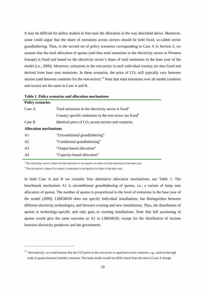
Table 1. Policy scenarios and allocation mechanisms

Policy scenarios

Case A Total emissions in the electricity sector is fixeda

Country specific emissions in the rest-sector are fixedb

Case B Identical price of CO2 across sectors and countries

Allocation mechanisms

A1 “Unconditional grandfathering”

A2 “Conditional grandfathering”

A3 “Output-based allocation”

A4 “Capacity-based allocation”

a The electricity sector’s share of total emissions is set equal to its share of total emissions in the base year.

b The rest-sector’s share of a country’s emissions is set equal to its share in the base year.

In both Case A and B we consider four alternative allocation mechanisms, see Table 1. The

benchmark mechanism A1 is unconditional grandfathering of quotas, i.e., a variant of lump sum

allocation of quotas. The number of quotas is proportional to the level of emissions in the base year of

the model (2000). LIBEMOD does not specify individual installations, but distinguishes between

different electricity technologies, and between existing and new installations. Thus, the distribution of

quotas is technology-specific and only goes to existing installations. Note that full auctioning of

quotas would give the same outcome as A1 in LIBEMOD, except for the distribution of income

between electricity producers and the government.

12 Alternatively, we could assume that the CO2-price in the rest-sector is equalized across countries, e.g., realized through

trade in quotas between member countries. The main results would not differ much from the ones in Case A though.

20

The second mechanism A2 also assumes that quotas are grandfathered to existing firms. However,

quotas will be withdrawn from installations that shut down (i.e., do not maintain) their capacity. If, for

example, maintained capacity of existing coal power producers in a country is reduced by k percent

compared to the base year level, coal power producers will only receive (100-k) percent of the quotas

they would have received if they did not shut down capacity. Obviously, this allocation mechanism

gives increased incentives to maintain production capacity compared to the benchmark mechanism, as

the producers lose valuable quotas if they shut down capacity.

The third mechanism A3 does not involve any grandfathering. Instead, quotas are distributed in

proportion to current production, i.e., output-based allocation, which was examined in the analytical

model in Section 2. As shown in Section 2, this allocation mechanism acts as an implicit production

subsidy, and hence gives increased incentives to produce electricity. Note, however, that only fossil-

based electricity production receives quotas, in line with e.g. the EU ETS.

Finally, the fourth mechanism A4 assumes that quotas are distributed in proportion to maintained

capacity. Thus, similar to A3, mechanism A4 is connected to present activity, not to the past. This

mechanism will give higher incentives to invest in and maintain production capacity, but not to

produce (at least not directly). Again, only fossil-based power plants receive quotas.

Comparing with the allocation rules in the EU ETS, allocation in the first two periods (2005-2007 and

2008-2012) has varied across member states and sectors, but in general it has been a mixture of

allocation mechanism A2 for existing installations and A4 for new installations and capacity

expansions at existing installations.13 In the next period (2013-2020), allocation rules are mostly

harmonized across the EU. Electricity producers will as a default no longer receive allowances, but ten

of the new member states (EU-12 minus Slovakia and Slovenia) have got an option to allocate a

limited number of allowances to electricity generators that have been in operation since (or had started

to invest before) the end of 2008. The member states can then choose between allocation mechanisms

similar to A2 or A4. Other sectors will still be given substantial amounts of free allowances (in all

member states), using a mixture of allocation mechanisms similar to A3 and A4.14

13 Allocation rules have not been harmonized across EU member states, so the comparison is only an approximation. For

instance, some countries have chosen different allocation parameters for investments in different power technologies,

whereas others have chosen equal parameters. Note that combining A2 for existing installations and A4 for new

installations (and capacity expansions) gives the same outcome as allocation mechanism A4 in our model simulations.

14 Allocation to an installation will be proportional to historic production level (2007-8), but adjusted whenever the operating

capacity is reduced or increased substantially. New installations will receive quotas in proportion to operating capacity.

21

One interpretation of our results is therefore that they may provide insight into how the links between

the EU ETS and the power market in Western Europe may change when going from the second to the

third period (by comparing A2 and A4 with A1). Moreover, it demonstrates how the power market

could have been affected if electricity generators had been treated in the same way as other industries

in the EU ETS (by considering A3 and A4).

5 Numerical results

5.1 Base case 2010

Before we examine the effects of the different policies, let us take a brief look at the base case scenario

in 2010. Remember that the model is calibrated to the data year 2000. Compared to that year, the

model accounts for growth in demand due to economic growth from 2000 to 2010. Moreover, existing

capacities in electricity production and transmission in 2000 are depreciated at a fixed annul rate. On

the other hand, profitable investments in electricity production and transmission of electricity and

natural gas are assumed to be in place in 2010.15 Still, we should not expect the base case scenario for

2010 to be identical to the actual market situation in 2010, as there are a number of factors (including

new policies) influencing the market that is not accounted for in the base case of the model.

In the base case scenario for 2010, CO2-emissions in Western Europe are 25 percent above the joint

annual Kyoto target for the years 2008-12. The electricity sector accounts for about one third of

emissions in Western Europe, cf. Table 2 below. The average whole price of electricity is 40 Euro per

MWh (see Table 3), with national prices varying in the range 32-43 Euro per MWh (see the Appendix

for country details). The average whole prices of steam coal, natural gas and oil are respectively 65,

146 and 249 Euro per toe.16

Partly due to relatively low coal prices, coal power production grows substantially compared to 2000,

see Table 4 (remember that the base case assumes no new climate policies after 2000). The market

share of coal power is thus 37 percent in the base case. Nuclear power, gas power and hydro power

have market shares of respectively 24, 21 and 14 percent, whereas other renewables have merely 5

15 The supply functions for gas to Europe have also been adjusted from 2000 to 2010.

16 Coal and electricity prices in the base case scenario are quite close to actual price levels in 2010, whereas gas and oil prices

were significantly higher in reality. Of course, in 2010 energy prices were influenced by the EU ETS, so it may seem more

relevant to compare actual 2010-prices with the policy scenarios below.

22

percent. Oil power is not profitable. Around one quarter of power production in 2010 comes from new

plants, i.e., plants built after 2000.

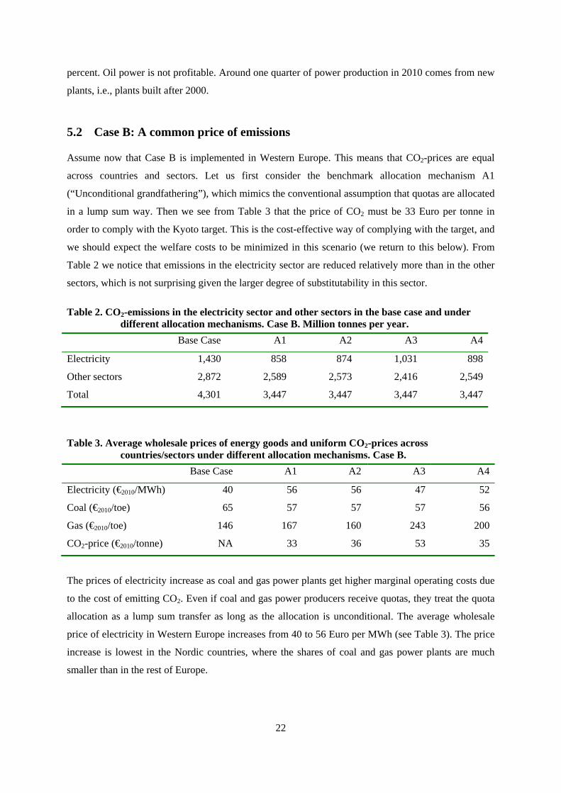
5.2 Case B: A common price of emissions

Assume now that Case B is implemented in Western Europe. This means that CO2-prices are equal

across countries and sectors. Let us first consider the benchmark allocation mechanism A1

(“Unconditional grandfathering”), which mimics the conventional assumption that quotas are allocated

in a lump sum way. Then we see from Table 3 that the price of CO2 must be 33 Euro per tonne in

order to comply with the Kyoto target. This is the cost-effective way of complying with the target, and

we should expect the welfare costs to be minimized in this scenario (we return to this below). From

Table 2 we notice that emissions in the electricity sector are reduced relatively more than in the other

sectors, which is not surprising given the larger degree of substitutability in this sector.

Table 2. CO2-emissions in the electricity sector and other sectors in the base case and under different allocation mechanisms. Case B. Million tonnes per year.

Base Case A1 A2 A3 A4

Electricity 1,430 858 874 1,031 898

Other sectors 2,872 2,589 2,573 2,416 2,549

Total 4,301 3,447 3,447 3,447 3,447

Table 3. Average wholesale prices of energy goods and uniform CO2-prices across countries/sectors under different allocation mechanisms. Case B.

Base Case A1 A2 A3 A4

Electricity (€2010/MWh) 40 56 56 47 52

Coal (€2010/toe) 65 57 57 57 56

Gas (€2010/toe) 146 167 160 243 200

CO2-price (€2010/tonne) NA 33 36 53 35

The prices of electricity increase as coal and gas power plants get higher marginal operating costs due

to the cost of emitting CO2. Even if coal and gas power producers receive quotas, they treat the quota

allocation as a lump sum transfer as long as the allocation is unconditional. The average wholesale

price of electricity in Western Europe increases from 40 to 56 Euro per MWh (see Table 3). The price

increase is lowest in the Nordic countries, where the shares of coal and gas power plants are much

smaller than in the rest of Europe.

23

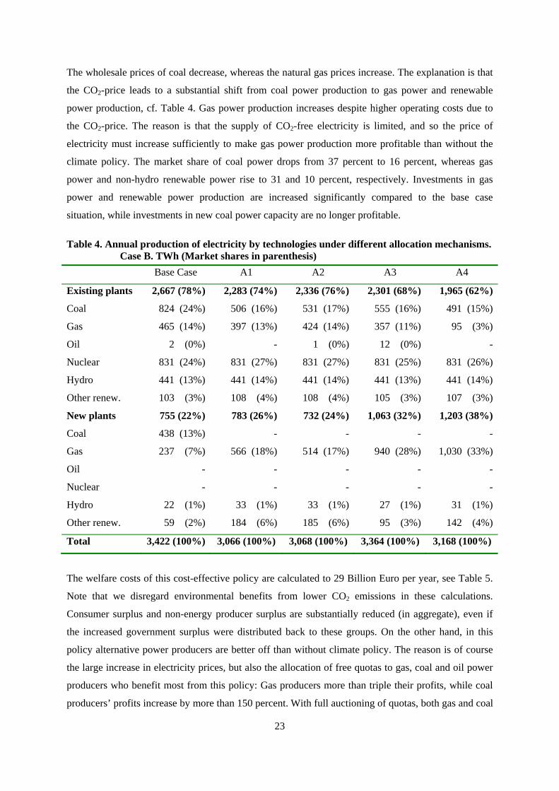
The wholesale prices of coal decrease, whereas the natural gas prices increase. The explanation is that

the CO2-price leads to a substantial shift from coal power production to gas power and renewable

power production, cf. Table 4. Gas power production increases despite higher operating costs due to

the CO2-price. The reason is that the supply of CO2-free electricity is limited, and so the price of

electricity must increase sufficiently to make gas power production more profitable than without the

climate policy. The market share of coal power drops from 37 percent to 16 percent, whereas gas

power and non-hydro renewable power rise to 31 and 10 percent, respectively. Investments in gas

power and renewable power production are increased significantly compared to the base case

situation, while investments in new coal power capacity are no longer profitable.

Table 4. Annual production of electricity by technologies under different allocation mechanisms. Case B. TWh (Market shares in parenthesis)

Base Case A1 A2 A3 A4

Existing plants 2,667 (78%) 2,283 (74%) 2,336 (76%) 2,301 (68%) 1,965 (62%)

Coal 824 (24%) 506 (16%) 531 (17%) 555 (16%) 491 (15%)

Gas 465 (14%) 397 (13%) 424 (14%) 357 (11%) 95 (3%)

Oil 2 (0%) - 1 (0%) 12 (0%) -

Nuclear 831 (24%) 831 (27%) 831 (27%) 831 (25%) 831 (26%)

Hydro 441 (13%) 441 (14%) 441 (14%) 441 (13%) 441 (14%)

Other renew. 103 (3%) 108 (4%) 108 (4%) 105 (3%) 107 (3%)

New plants 755 (22%) 783 (26%) 732 (24%) 1,063 (32%) 1,203 (38%)

Coal 438 (13%) - - - -

Gas 237 (7%) 566 (18%) 514 (17%) 940 (28%) 1,030 (33%)

Oil - - - - -

Nuclear - - - - -

Hydro 22 (1%) 33 (1%) 33 (1%) 27 (1%) 31 (1%)

Other renew. 59 (2%) 184 (6%) 185 (6%) 95 (3%) 142 (4%)

Total 3,422 (100%) 3,066 (100%) 3,068 (100%) 3,364 (100%) 3,168 (100%)

The welfare costs of this cost-effective policy are calculated to 29 Billion Euro per year, see Table 5.

Note that we disregard environmental benefits from lower CO2 emissions in these calculations.

Consumer surplus and non-energy producer surplus are substantially reduced (in aggregate), even if

the increased government surplus were distributed back to these groups. On the other hand, in this

policy alternative power producers are better off than without climate policy. The reason is of course

the large increase in electricity prices, but also the allocation of free quotas to gas, coal and oil power

producers who benefit most from this policy: Gas producers more than triple their profits, while coal

producers’ profits increase by more than 150 percent. With full auctioning of quotas, both gas and coal

24

producers would stand to lose, but power producers as a group would still gain as producers using

CO2-free energy would increase their profits by 60 percent. Consumers and non-energy producers

would still lose out even if they get the revenues from auctioning of quotas.

Table 5. Economic welfare changes compared to Base Case. Case B. Billion Euro per year

A1 A2 A3 A4

Consumer and non-energy producer surplus -151 -158 -190 -152

Power producer surplus 43 44 5 21

Other energy producer surplus and trade surplus 3 0 22 11

Government surplus 77 83 115 80

Total -29 -30 -49 -40

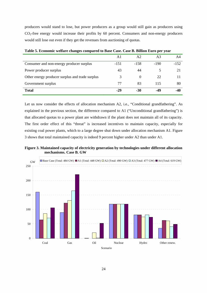
Let us now consider the effects of allocation mechanism A2, i.e., “Conditional grandfathering”. As

explained in the previous section, the difference compared to A1 (“Unconditional grandfathering”) is

that allocated quotas to a power plant are withdrawn if the plant does not maintain all of its capacity.

The first order effect of this “threat” is increased incentives to maintain capacity, especially for

existing coal power plants, which to a large degree shut down under allocation mechanism A1. Figure

3 shows that total maintained capacity is indeed 9 percent higher under A2 than under A1.

Figure 3. Maintained capacity of electricity generation by technologies under different allocation mechanisms. Case B. GW

0

50

100

150

200

250

Coal Gas Oil Nuclear Hydro Other renew.

Scenario

GW Base Case (Total: 484 GW) A1 (Total: 448 GW) A2 (Total: 490 GW) A3 (Total: 477 GW) A4 (Total: 619 GW)

25

With more capacity available, production of electricity from existing plants also increases compared to

the cost-effective outcome in A1.17 This is seen in Table 6. We notice that especially supply from old

coal power plants increases in A2 compared to A1. This crowds out some production from new gas

power plants, so that total production of electricity is approximately the same under A1 and A2. The

share of coal is slightly higher in A2, whereas the share of gas is slightly lower.

Consistent with almost unchanged production, the price of electricity is also almost the same in A2 as

in A1.18 The average price of gas decreases by four percent. On the other hand, the price of CO2

increases by about nine percent as the allocation mechanism stimulates capacity maintenance and thus

production (as a first order effect), and so the price must increase in order to comply with the overall

target. Moreover, the electricity sector now has a bigger share of total emissions as the higher CO2-

price reduces emissions in the rest-sector.

The costs of complying with the overall emissions target increase by five percent (relative to A1)

when the quota allocation to power plants is conditioned on maintained capacity. Consumers and non-

energy producers are worse off due to a higher CO2-tax, but this has its counterpart in higher

government tax revenues. Gas producers lose profits as reduced gas power production leads to lower

gas prices, whereas power plants using lignite are the main winners among power producers. The

higher total welfare costs are due to the fact that more expensive power plants (accounting for the

shadow costs of CO2-emissions) are employed to produce almost the same amount of electricity. The

cost differential is moderated by the fact that there are beneficial terms-of-trade effects for Western

Europe as whole in A2, related to lower import prices of natural gas (compared to A1). The opposite is

the case in A3 and A4, cf. the gas prices in Table 3.

The first two allocation mechanisms allocate quotas based on historic emissions. The other two

mechanisms allocate quotas based on plants’ current activity levels, i.e., in proportion to either output

(A3) or (maintained) capacity (A4). Consequently, the latter two mechanisms give enhanced

incentives to respectively produce (A3) or maintain/invest in power capacity (A4) for the fossil-based

plants that receive quotas.

17 Not all the maintained capacity is used, however. For instance, oil power capacities are maintained in all countries under

A2, but only used in one country.

18 Both total production and the average price increase marginally, which may seem inconsistent. The explanation is that the

average price is a weighted average over four time periods and 16 regions. Thus, the price falls in some periods/regions

and increases in other periods/regions.

26

The first order effect of allocation mechanism A3 (compared to A1) is to increase electricity

production in coal and gas power plants. This leads to lower electricity prices, whereas the price of

CO2 must increase in order to comply with the overall emissions target. These price effects reduce the

profitability of coal and gas power plants, and the higher CO2-price is clearly most harmful for (old)

coal power producers. As a consequence, output-based allocation (A3) is most favourable for gas

power plants, which explains why gas power increases its market share from 31 percent (under A1) to

39 percent (under A3), cf. Table 4. This is consistent with the analytical results derived in Section 2,

showing that the least emission-intensive producers will benefit from output-based allocation.

The increased gas power production comes from new gas power plants, whereas old gas power plants

actually produce less than in A1. The reason is that new plants are more effective than existing plants,

and hence emit less CO2 per unit kWh produced. The market share of coal power is about the same, as

the effect of higher CO2-price more or less matches the effect of increased production incentives.

Renewable electricity production drops, however, due to lower electricity prices (see below).

Increased investments in gas power capacity crowds out investments in especially wind power

capacity. Total power production increases by 10 percent compared to A1. The CO2-price ends up 60

percent higher in A3 than in A1, which is also consistent with the analytical results in Section 2.

As indicated already, the price of electricity is reduced even more in A3 compared to A1 and A2; in

A3 the price of electricity is 15 percent lower than in A1. There are two reasons why the price is lower

(and production higher) in A3 than in A2. First, A3 has the highest price of CO2, which is due to the

strong incentives to produce and thus emit under this allocation mechanism. A higher CO2-price

means that less emissions take place in the rest-sector, and thus more emissions are allowed in the

electricity sector (see Table 2). Second, the emission-intensity is reduced in A3 compared to A2, as

allocation mechanism A2 mostly favour old coal power plants, while allocation mechanism A3 mostly

favour new gas power plants. Combined, these two factors imply that production is higher and

electricity prices lower in A3 than in A2.

The economic welfare costs of allocation mechanism A3 are significantly higher than under A1 and

A2, i.e., 70 percent higher than under A1. This might seem counter-intuitive inasmuch as more and

cleaner electricity is produced under A3. The explanation is that the implicit subsidy provided by the

allocation mechanism A3 stimulates more supply from more expensive (though somewhat cleaner)

power plants. Someone has to pay for these higher costs of supply, and we notice that the group of

power producers is significantly worse off with this allocation mechanism despite the implicit

production subsidy, see Table 5. Even the group of gas producers loses profits despite the large

expansion of gas power, as new gas power plants to some degree crowd out old plants. Consumers are

27

also worse off under A3 than under A1, but not if extra government surplus is distributed to the

consumers. Then they are more or less indifferent, due to a combination of lower electricity prices and

substantially higher gas prices (vis-à-vis A1).

The last allocation mechanism A4 makes it more profitable to maintain existing capacity and invest in

new capacity, but not necessarily to produce electricity. Still, when more capacity is available,

production will typically also increase as the marginal cost of producing one more unit is lower when

investment costs are sunk. As shown in Figure 3, total power production capacity is indeed highest

under this allocation mechanism. In particular, investments in new gas power plants are increased

relative to all other scenarios, including A3. In addition, much more of the existing coal and gas

capacity are maintained.

From Table 4 we notice that total electricity production increases slightly compared to A1 and A2

(grandfathered allocation), i.e., by three percent, but is lower than under output-based allocation (A3),

which stimulates production directly. Production from new gas power plants is, however, higher under

A4 than under A3, whereas production from existing gas and coal power plants is reduced compared

to all other scenarios. The reduction is particularly strong for existing gas power plants. The reason is

that increased supply from new gas power plants harms existing gas power plants (which are less

efficient than the new ones) via three channels: Higher gas prices, higher CO2-prices, and lower

electricity prices.

The price of CO2 under A4 lies between the price level under A1 and A2. The price of electricity,

however, is six percent lower than under A1 and A2, which is consistent with the higher level of

production. The welfare costs are substantially lower with allocation mechanism A4 than with A3. The

main reason is the much higher CO2 price under A3, which substantially shifts emission reductions

from the electricity sector to the other sectors (compare with the cost-effective solution A1 in Table 2).

Nevertheless, the welfare costs are 40 percent higher than under A1, mostly because it leads to

excessive levels of maintained power capacity.

Looking at the increase in the average electricity price (relative to base case) and the CO2-price under

the four different allocation mechanisms, we notice that the relationship between these two varies a

lot. Under the cost-effective allocation mechanism A1, the ratio is 0.47 tonne CO2 per MWh.19 The

corresponding ratios under A2, A3 and A4 are 0.43, 0.13 and 0.34 respectively. This illustrates quite

clearly that the so-called pass-through of CO2-prices into the electricity price does not only depend on

19 (56 €/MWh – 40 €/MWh) / (33 €/ton CO2) = 0.47 ton CO2 per MWh

28

whether coal or gas power (old or new) is on the margin, but also on the way quotas are allocated to

the power producers, working through the multimarket equilibria, notably the markets for fuel inputs.

With output-based allocation, the pass-through rate (0.13) is in fact only one-third of the emission

intensity of new gas power plants (0.38 tonne CO2 per MWh), and one sixth of the emission intensity

of new coal power plants (0.78 tonne CO2 per MWh).

5.3 Case A: Fixed sectoral emissions

Assume now instead that Case A is implemented, which means that a certain share of the overall

emissions target is allocated to the electricity sector, irrespective of allocation mechanism. This share

is set equal to the sector’s share of emissions in the base year, i.e., 27 percent. We notice from Table 2

that the share is lower than in the base case scenario of 2010 (33 percent), but it is slightly higher than

in the cost-effective emission reduction scenario described above (Case B-A1), where the electricity

sector accounted for 25 percent of emissions.

Most of the qualitative insight reached above for Case B, such as the differences between the four

allocation mechanisms, carries over to Case A. Thus, we will not go into all the details here. We will

rather highlight the main differences between Case A and B, and refer the interested reader to the

tables in Appendix B.

With lump sum allocation of quotas (A1: “Unconditional grandfathering”), the price of CO2 in the

electricity sector is about 29 Euro per tonne (see Table 6), i.e., 13 percent lower than with equal CO2-

price across all sectors (Case B-A1). On the other hand, for the other sectors the weighted average

price of CO2 across Western Europe is 50 Euro per tonne. The explanation is of course that it is less

costly to reduce emissions in the power sector, where more substitution possibilities are present. This

is well known to policy makers in Europe, who seem to put more ambitious targets on this sector than

on other sectors. Note, however, that the CO2 price for the other sectors varies quite substantially

across countries due to different emission targets and different costs of reducing emissions (e.g.,

because of differences in fuel mix and industry structure).

Under allocation mechanism A3 the CO2 price is higher in the electricity sector than in the rest of the

economy, and we notice from Table 6 that the quota price is more than twice as high under A3 than

under A1. In the Case A scenarios, emissions in the electricity sector cannot increase, and thus the

price of emissions has to increase even more under Case A-A3 than under Case B-A3.

29

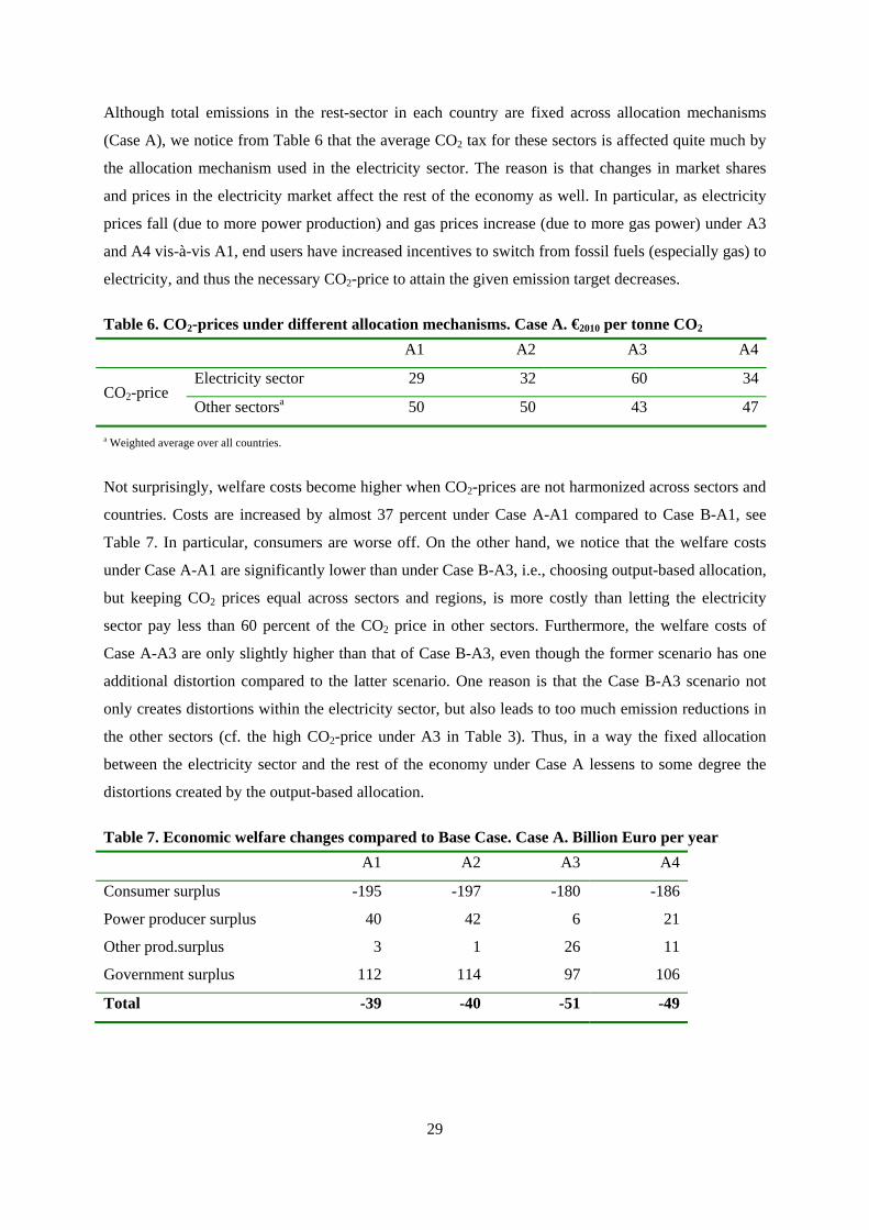
Although total emissions in the rest-sector in each country are fixed across allocation mechanisms

(Case A), we notice from Table 6 that the average CO2 tax for these sectors is affected quite much by

the allocation mechanism used in the electricity sector. The reason is that changes in market shares

and prices in the electricity market affect the rest of the economy as well. In particular, as electricity

prices fall (due to more power production) and gas prices increase (due to more gas power) under A3

and A4 vis-à-vis A1, end users have increased incentives to switch from fossil fuels (especially gas) to

electricity, and thus the necessary CO2-price to attain the given emission target decreases.

Table 6. CO2-prices under different allocation mechanisms. Case A. €2010 per tonne CO2

A1 A2 A3 A4

CO2-price Electricity sector 29 32 60 34

Other sectorsa 50 50 43 47

a Weighted average over all countries.

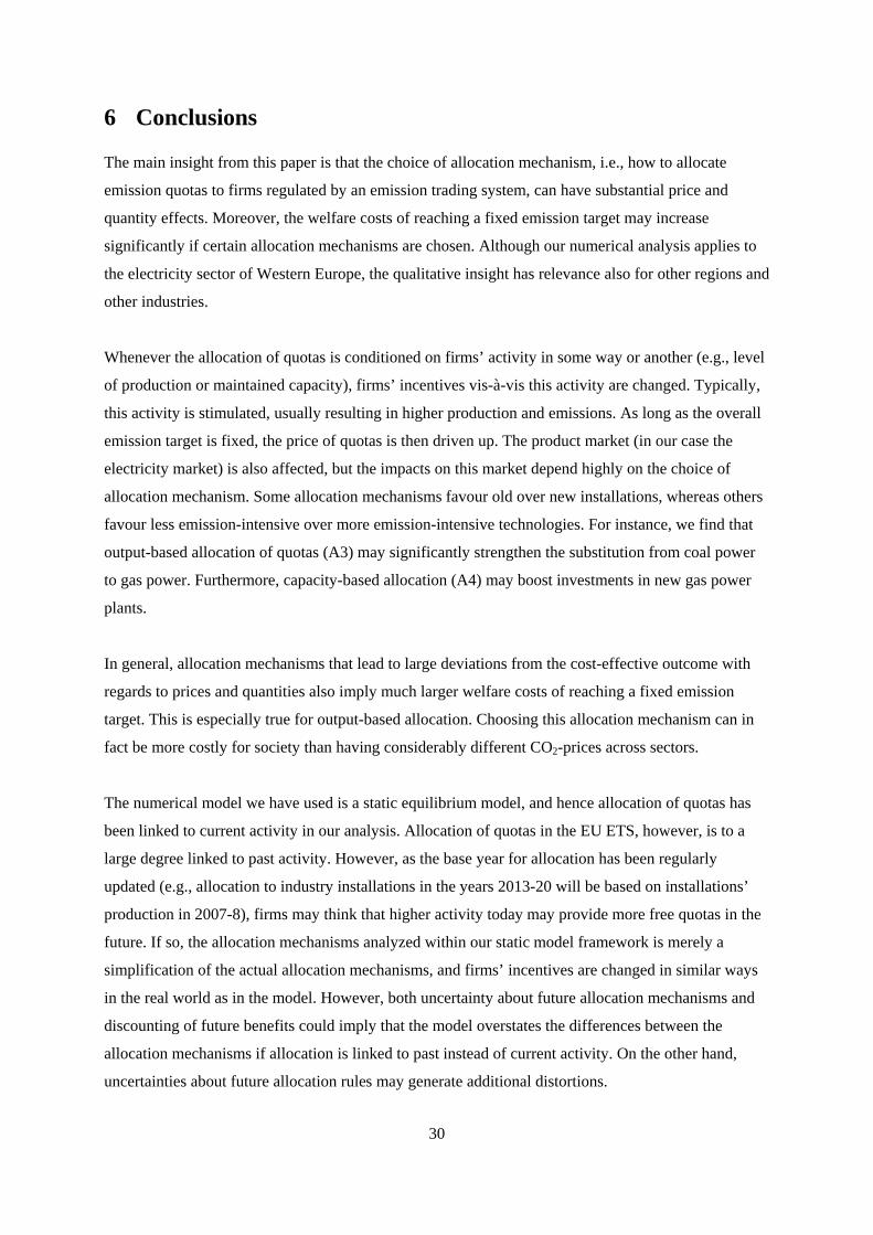
Not surprisingly, welfare costs become higher when CO2-prices are not harmonized across sectors and

countries. Costs are increased by almost 37 percent under Case A-A1 compared to Case B-A1, see

Table 7. In particular, consumers are worse off. On the other hand, we notice that the welfare costs

under Case A-A1 are significantly lower than under Case B-A3, i.e., choosing output-based allocation,

but keeping CO2 prices equal across sectors and regions, is more costly than letting the electricity

sector pay less than 60 percent of the CO2 price in other sectors. Furthermore, the welfare costs of

Case A-A3 are only slightly higher than that of Case B-A3, even though the former scenario has one

additional distortion compared to the latter scenario. One reason is that the Case B-A3 scenario not

only creates distortions within the electricity sector, but also leads to too much emission reductions in

the other sectors (cf. the high CO2-price under A3 in Table 3). Thus, in a way the fixed allocation

between the electricity sector and the rest of the economy under Case A lessens to some degree the

distortions created by the output-based allocation.

Table 7. Economic welfare changes compared to Base Case. Case A. Billion Euro per year

A1 A2 A3 A4

Consumer surplus -195 -197 -180 -186

Power producer surplus 40 42 6 21

Other prod.surplus 3 1 26 11

Government surplus 112 114 97 106

Total -39 -40 -51 -49

30

6 Conclusions

The main insight from this paper is that the choice of allocation mechanism, i.e., how to allocate

emission quotas to firms regulated by an emission trading system, can have substantial price and

quantity effects. Moreover, the welfare costs of reaching a fixed emission target may increase

significantly if certain allocation mechanisms are chosen. Although our numerical analysis applies to

the electricity sector of Western Europe, the qualitative insight has relevance also for other regions and

other industries.

Whenever the allocation of quotas is conditioned on firms’ activity in some way or another (e.g., level

of production or maintained capacity), firms’ incentives vis-à-vis this activity are changed. Typically,

this activity is stimulated, usually resulting in higher production and emissions. As long as the overall

emission target is fixed, the price of quotas is then driven up. The product market (in our case the

electricity market) is also affected, but the impacts on this market depend highly on the choice of

allocation mechanism. Some allocation mechanisms favour old over new installations, whereas others

favour less emission-intensive over more emission-intensive technologies. For instance, we find that

output-based allocation of quotas (A3) may significantly strengthen the substitution from coal power

to gas power. Furthermore, capacity-based allocation (A4) may boost investments in new gas power

plants.

In general, allocation mechanisms that lead to large deviations from the cost-effective outcome with

regards to prices and quantities also imply much larger welfare costs of reaching a fixed emission

target. This is especially true for output-based allocation. Choosing this allocation mechanism can in

fact be more costly for society than having considerably different CO2-prices across sectors.

The numerical model we have used is a static equilibrium model, and hence allocation of quotas has

been linked to current activity in our analysis. Allocation of quotas in the EU ETS, however, is to a

large degree linked to past activity. However, as the base year for allocation has been regularly

updated (e.g., allocation to industry installations in the years 2013-20 will be based on installations’

production in 2007-8), firms may think that higher activity today may provide more free quotas in the

future. If so, the allocation mechanisms analyzed within our static model framework is merely a

simplification of the actual allocation mechanisms, and firms’ incentives are changed in similar ways

in the real world as in the model. However, both uncertainty about future allocation mechanisms and

discounting of future benefits could imply that the model overstates the differences between the

allocation mechanisms if allocation is linked to past instead of current activity. On the other hand,

uncertainties about future allocation rules may generate additional distortions.

31

As explained above, the electricity sector will as a general rule no longer receive quotas in the EU

ETS from 2013, but most of the new member states (EU-12) will nevertheless continue to allocate

quotas to their power installations. Our welfare results may provide some indications about the

benefits of departing from free allocation to this sector, or alternatively, the costs of continuing this

practice. Note, however, that the allocation mechanism used for this sector in the EU ETS is not the

most costly one in our analysis (A3), but rather a mixture of two others (A2 and A4). On the other

hand, with different allocation rules across countries, additional inefficiencies may arise.

The remaining sectors of the EU ETS will still receive substantial amounts of quotas, using a mixture

of allocation mechanism A3 and A4. Our analysis may suggest that this could be quite costly for the

EU compared to pure auctioning. However, the objective of free allocation to these sectors is to

prevent carbon leakage (cf. Böhringer et al., 2010). Thus, it is difficult to judge in general whether the

extra costs showing up in our analysis are higher or lower than the eventual benefits of reduced

leakage. Still, our results suggest that free allocation of quotas to sectors with little or no carbon

leakage is suboptimal.

References

Aune, F.R., R. Golombek, S.A.C. Kittelsen and K.E. Rosendahl (2008): Liberalizing European

Energy Markets. An Economic Analysis, Cheltenham, UK: Edward Elgar Publishing.

Bode, S. (2006): Multi-period emissions trading in the electricity sector—winners and lowers, Energy

Policy 34, 680-691.

Bunn, D. and C. Fezzi (2007): Interaction of European Carbon Trading and Energy Prices, Fondazione

Eni Enrico Mattei Working Paper: 123.

Burtraw D, D. Kahn and K. Palmer (2006): CO2 allowance allocation in the regional greenhouse gas

initiative and the effect on electricity investors, The Electricity Journal 19 (2), 79-90.

Burtraw, D. and K. Palmer (2008): Compensation Rules for Climate Policy in the Electricity Sector,

Journal of Policy Analysis and Management 27(4), 819-847.

Böhringer, C. and A. Lange (2005a): Economic implications of alternative allocation schemes for

emission allowances, Scandinavian Journal of Economics 107, 563-581.

32

Böhringer, C. and A. Lange (2005b): On the design of optimal grandfathering schemes for emission

allowances, European Economic Review 49, 2041-2055.

Böhringer, C., C. Fischer and K.E. Rosendahl (2010): The Global Effects of Subglobal Climate

Policies, The B.E. Journal of Economic Analysis & Policy 10 (2) (Symposium), Article 13.

Böhringer, C. and K.E. Rosendahl (2010): Green Serves the Dirtiest. On the Interaction between Black

and Green Quotas, Journal of Regulatory Economics 37, 316–325.

Chen, Y., J. Sijm, B.F. Hobbs and W. Lise (2008): Implications of CO2 emissions trading for short-run

electricity market outcomes in northwest Europe, Journal of Regulatory Economics 34(3), 251-281.

Ellerman, A.D. (2008): New Entrant and Closure Provisions: How do they Distort? The Energy

Journal, Special Issue to Acknowledge the Contribution of Campbell Watkins to Energy Economics,

63-76.

Fell, H. (2010): EU-ETS and Nordic Electricity: A CVAR Analysis, The Energy Journal 31(2), 1-26.

Fischer, C. (2001): Rebating Environmental Policy Revenues: Output-Based Allocations and Tradable

Performance Standards, RFF Discussion Paper 01–22, Resources for the Future.

Fischer, C. and A. K. Fox (2007): Output-based allocation of emissions permits for mitigating tax and

trade interactions, Land Economics 83, 575-599.

Goulder, L. H. (1995): Environmental taxation and the double dividend: A reader’s guide,

International Tax and Public Finance 2, 157-183.

House of Representatives (2009): The American Clean Energy and Security Act (H.R. 2454), Bill

Text as Passed by House of Representatives.

http://energycommerce.house.gov/Press_111/20090701/hr2454_house.pdf

Kirat, D. and I. Ahamada (2011): The impact of the European Union emission trading scheme on the

electricity-generation sector, Energy Economics, doi:10.1016/j.eneco.2011.01.012.

33

Lise, W., J. Sijm and B. F. Hobbs (2010): The Impact of the EU ETS on Prices, Profits and Emissions

in the Power Sector: Simulation Results with the COMPETES EU20 Model, Environmental and

Resource Economics 47, 23–44.

Montgomery, W. D. (1972): Markets in licenses and efficient pollution control programs, Journal of

Economic Theory 5, 395-418.

Neuhoff, K., K. Keats Martinez and M. Sato (2006): Allocation, incentives and distortions: The impact

of EU ETS emissions allowance allocations to electricity sector, Climate Policy 6, 73-91.

Newbery, D.M. (2008): Climate change policy and its effect on market power in the gas market,

Journal of the European Economic Association 6(4), 727–751.

Rosendahl, K.E. (2008): Incentives and quota prices in an emissions trading scheme with updating,

Journal of Environmental Economics and Management 56, 69-82.

Rosendahl, K.E. and H. Storrøsten (2011a): Emissions trading with updated allocation: Effects on

entry/exit and distribution, Environmental and Resource Economics 49, 243-261.

DOI 10.1007/s10640-010-9432-z

Rosendahl, K.E. and H. Storrøsten (2011b): Output-based allocation and investment in clean

technologies, Discussion Papers No. 644, Statistics Norway.

http://www.ssb.no/publikasjoner/pdf/dp644.pdf

Sijm, J.P.M., K. Neuhoff and Y. Chen (2006): CO2 cost pass through and windfall profits in the power

sector, Climate Policy 6(1), 49–72.

Simshauser, P. and T. Doan (2009): Emissions Trading, Wealth Transfers and the Wounded Bull

Scenario in Power Generation, The Australian Economic Review 42(1), 64–83.

Sterner, T. and A. Muller (2008): Output and Abatement Effects of Allocation Readjustment in Permit

Trade, Climatic Change 86, 33-49.

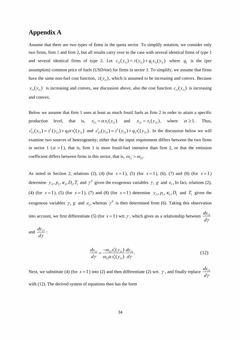
34

Appendix A

Assume that there are two types of firms in the quota sector. To simplify notation, we consider only

two firms, firm 1 and firm 2, but all results carry over to the case with several identical firms of type 1

and several identical firms of type 2. Let 1 1 1 1 1 1( ) ( ) ( )i i i i ic y z y q x y where 1q is the (per

assumption) common price of fuels (USD/toe) for firms in sector 1. To simplify, we assume that firms

have the same non-fuel cost function, 1( )iz y , which is assumed to be increasing and convex. Because

1 1( )i ix y is increasing and convex, see discussion above, also the cost function 1 1( )i ic y is increasing

and convex.

Below we assume that firm 1 uses at least as much fossil fuels as firm 2 in order to attain a specific

production level, that is, 11 1 11( )x x y and 21 1 21( )x x y , where 1. Thus,

11 11 11 1 1 11( ) ( ) ( )c y z y q x y and 21 21 21 1 1 21( ) ( ) ( )c y z y q x y . In the discussion below we will

examine two sources of heterogeneity; either that the input requirement differs between the two firms

in sector 1 ( 1 ), that is, firm 1 is more fossil-fuel intensive than firm 2, or that the emission

coefficient differs between firms in this sector, that is, 11 21.

As noted in Section 2, relations (2), (4) (for 1s ), (5) (for 1s ), (6), (7) and (8) (for 1s )

determine 1 1 1 1 1, , , ,iy p D T and 0 given the exogenous variables , g and 1 ,e In fact, relations (2),

(4) (for 1s ), (5) (for 1s ), (7) and (8) (for 1s ) determine 1 1 1 1, , ,iy p D and 1T given the

exogenous variables , g and 1 ,e whereas 0 is then determined from (6). Taking this observation

into account, we first differentiate (5) (for 1s ) wrt. , which gives us a relationship between 11dy

d

and 21dy

d:

11 21 1 21 21

11 1 11

( ).

( )

dy x y dy

d x y d

(12)

Next, we substitute (4) (for 1s ) into (2) and then differentiate (2) wrt. , and finally replace 11dy

d

with (12). The derived system of equations then has the form

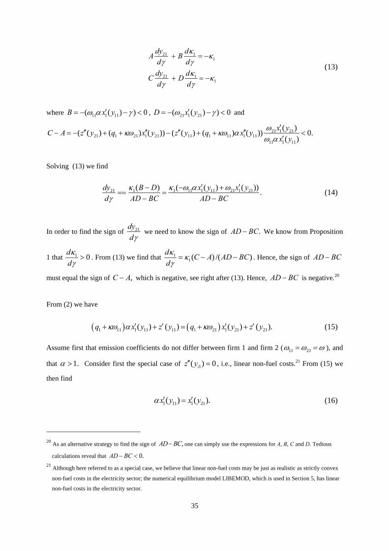
35

21 11

21 11

dy dA B

d d

dy dC D

d d

(13)

where 11 1 11( ( ) ) 0B x y , 21 1 21( ( ) ) 0D x y and

21 1 2121 1 21 1 21 11 1 11 1 11

11 1 11

( )( ( ) ( ) ( )) ( ( ) ( ) ( )) 0.

( )

x yC A z y q x y z y q x y

x y

Solving (13) we find

21 1 1 11 1 11 21 1 21( ) ( ( ) ( )).

dy B D x y x y

d AD BC AD BC

(14)

In order to find the sign of 21dy

d we need to know the sign of .AD BC We know from Proposition

1 that 1 0d

d

. From (13) we find that 1

1( ) /( )d

C A AD BCd

. Hence, the sign of AD BC

must equal the sign of ,C A which is negative, see right after (13). Hence, AD BC is negative.20

From (2) we have

1 11 1 11 11 1 21 1 21 21( ) ( ) ( ) ( ).q x y z y q x y z y (15)

Assume first that emission coefficients do not differ between firm 1 and firm 2 ( 11 21 ), and

that 1. Consider first the special case of 1( ) 0iz y , i.e., linear non-fuel costs.21 From (15) we

then find

1 11 1 21( ) ( ).x y x y (16)

20 As an alternative strategy to find the sign of ,AD BC one can simply use the expressions for A, B, C and D. Tedious

calculations reveal that 0.AD BC

21 Although here referred to as a special case, we believe that linear non-fuel costs may be just as realistic as strictly convex

non-fuel costs in the electricity sector; the numerical equilibrium model LIBEMOD, which is used in Section 5, has linear

non-fuel costs in the electricity sector.

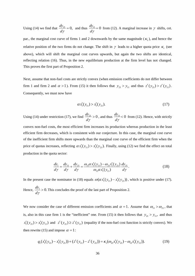
36

Using (14) we find that 21 0,dy

d and thus 11 0

dy

d from (12). A marginal increase in shifts, cet.

par., the marginal cost curve of firms 1 and 2 downwards by the same magnitude ( 1 ), and hence the

relative position of the two firms do not change. The shift in leads to a higher quota price 1 (see

above), which will shift the marginal cost curves upwards, but again the two shifts are identical,

reflecting relation (16). Thus, in the new equilibrium production at the firm level has not changed.

This proves the first part of Proposition 2.

Next, assume that non-fuel costs are strictly convex (when emission coefficients do not differ between

firm 1 and firm 2 and 1 ). From (15) it then follows that 21 11y y and thus 21 11( ) ( )z y z y .

Consequently, we must now have

1 11 1 21( ) ( ).x y x y (17)

Using (14) under restriction (17), we find 21 0dy

d , and thus 11 0

dy

d from (12). Hence, with strictly

convex non-fuel costs, the most efficient firm increases its production whereas production in the least

efficient firm decreases, which is consistent with our conjecture. In this case, the marginal cost curve

of the inefficient firm shifts more upwards than the marginal cost curve of the efficient firm when the

price of quotas increases, reflecting 1 11 1 21( ) ( ).x y x y Finally, using (12) we find the effect on total

production in the quota sector:

1 11 21 11 1 11 21 1 21 21

11 1 11

( ) ( ).

( )

dy dy dy x y x y dy

d d d x y d

(18)

In the present case the nominator in (18) equals 1 11 1 21( ( ) ( ))x y x y , which is positive under (17).

Hence, 1 0.dy

d This concludes the proof of the last part of Proposition 2.

We now consider the case of different emission coefficients and 1. Assume that 11 21 , that

is, also in this case firm 1 is the “inefficient” one. From (15) it then follows that 21 11,y y and thus

1 21 1 11( ) ( )x y x y and 21 11( ) ( )z y z y (equality if the non-fuel cost function is strictly convex). We

then rewrite (15) and impose 1:

1 1 11 1 21 11 21 1 21 1 21 11 1 11( ( ) ( )) ( ( ) ( )) ( ( ) ( )).q x y x y z y z y x y x y (19)

37

From the discussion above we know that the left hand side of (19) is negative, and hence the right

hand side of (19) also has to be negative:

21 1 21 11 1 11( ) ( ).x y x y (20) Thus in the present case the nominator in (14) is negative and the nominator in (18) is positive. Hence,

21 0dy

d and 1 0.

dy

d Finally, using (12) we have 11 0

dy

d . This concludes the proof of

Proposition 3.

We now turn to the case of a common price of emissions in the two sectors. This case is defined by

relations (2) - (10), see discussion above. In order to find the equilibrium effects of a shift in , we

first use (10) to replace 1 and 2 with . Next, combining (5) - (9) and differentiating wrt. we

find

21 221 1 21 2 2

11

11 1 11

( ).

( )

dy dyx y x

dy d dd x y

(21)

Next, substituting (4) (for 2s ) into (3) and differentiating, we find a relationship between 2dy

d and

d

d

, which is then substituted into (21):

221 2 2

21 1 2111 2 2 2 2

11 1 11

( )( )

.( )

dy x dx y

dy d P c x d

d x y

(22)

We then substitute (4) (for 1s ) into (2) and differentiate, and then use (22) to substitute for 11dy

d.

The resulting system of equations has the same form as (13), but with different coefficients; , ,A B C

and .D We find that

22 2 1 1 11

11 1 11 21 1 2121 11 1 11 2 2 2 2

( ) ( ) ( )( ( ) ( ))

( )( )( )

x q x yx y x y

dy x y P c xB D

d AD BC AD BC

(23)

38

Further, using (22) we find that the effect on total production in the quota sector 1 11 21( )y y y is

221 2 2

11 1 11 21 1 211 11 1 11 2 2 2 2

11 1 11

( )( ( ) ( ))

( )( )

( )

dy x dx y x y

dy d x y P c x d

d x y

(24)

In order to sign the denominator in (23), we use the same type of argument as in the case of fixed

sectoral emissions: Solving the system of equations we find 11( ) /( )

dC A AD BC

d

. From

Proposition 4 we know that this derivative is positive. Moreover, it can be shown that 0C A and

hence 0.AD BC

We now consider the different cases of heterogeneous firms. Assume first that emission coefficients

do not differ between firm 1 and firm 2 ( 11 21 ), and that 1. Consider first the special

case of 1( ) 0,iz y that is, 1 11 1 21( ) ( )x y x y , see (16). Then the first term in the nominator of (23)

is zero. The second term in the nominator of (23) is always negative. Because we know that the

denominator in (23) is negative, see discussion above, we have shown that 21 0.dy

d Further, in our

case the first term in the nominator of (24) is zero, whereas the second term is always positive and the

denominator is positive. Hence, 1 0.dy

d Finally, from (22) we see that the first term in the nominator

is negative (this is the same term as in the case of fixed sectoral emissions), whereas the second term is

positive (this term reflects lower emissions in the tax sector, which opens up for more emissions, and

thus more production, in firm 1). Hence, the impact on production of firm 1 is ambiguous.

Next, consider the case of non-fuel costs being strictly convex when emission coefficients do not

differ between firm 1 and firm 2, and 1 . We then have 1 11 1 21( ) ( ),x y x y see (17). Then the

first term in the nominator of (23) is negative, and the first term in the nominator of (24) is positive.

From the discussion above it then follows that 21 0dy

d and 1 0.

dy

d Again, the impact on

production of firm 1 is ambiguous, see (22).

Finally, consider the case of different emission coefficients ( 11 21 ) and 1. We then have

21 1 21 11 1 11( ) ( ),x y x y see (20). Like in the previous case the first term in the nominator of (23) is

39

negative, and the first term in the nominator of (24) is positive. Hence, 21 0,dy

d 1 0

dy

d and the

impact on production of firm 1 is ambiguous. This concludes the proof of Proposition 5.

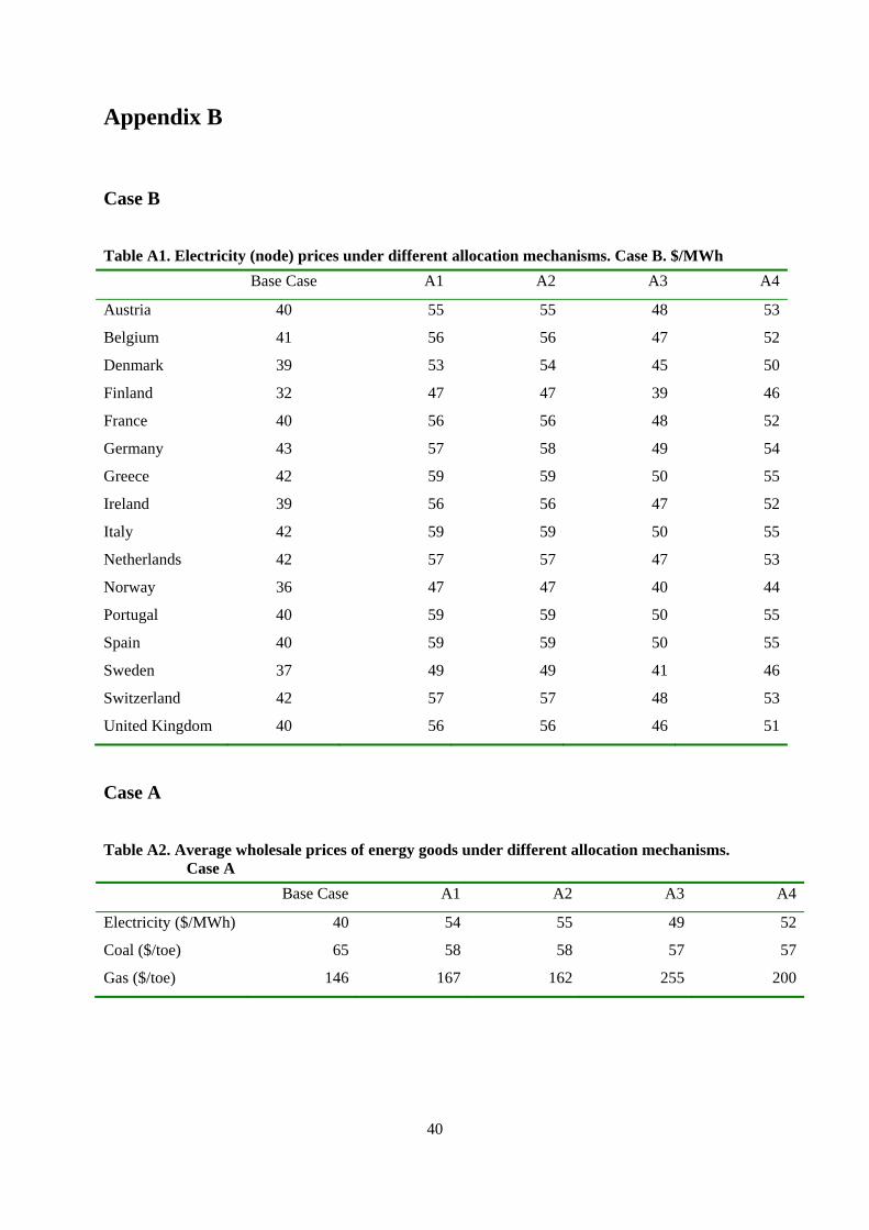
40

Appendix B

Case B

Table A1. Electricity (node) prices under different allocation mechanisms. Case B. $/MWh

Base Case A1 A2 A3 A4

Austria 40 55 55 48 53

Belgium 41 56 56 47 52

Denmark 39 53 54 45 50

Finland 32 47 47 39 46

France 40 56 56 48 52

Germany 43 57 58 49 54

Greece 42 59 59 50 55

Ireland 39 56 56 47 52

Italy 42 59 59 50 55

Netherlands 42 57 57 47 53

Norway 36 47 47 40 44

Portugal 40 59 59 50 55

Spain 40 59 59 50 55

Sweden 37 49 49 41 46

Switzerland 42 57 57 48 53

United Kingdom 40 56 56 46 51

Case A

Table A2. Average wholesale prices of energy goods under different allocation mechanisms. Case A

Base Case A1 A2 A3 A4

Electricity ($/MWh) 40 54 55 49 52

Coal ($/toe) 65 58 58 57 57

Gas ($/toe) 146 167 162 255 200

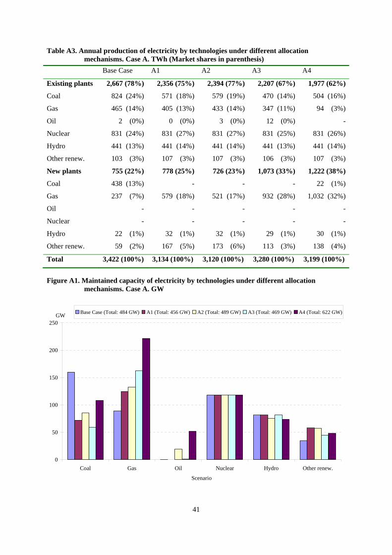
41

Table A3. Annual production of electricity by technologies under different allocation mechanisms. Case A. TWh (Market shares in parenthesis)

Base Case A1 A2 A3 A4

Existing plants 2,667 (78%) 2,356 (75%) 2,394 (77%) 2,207 (67%) 1,977 (62%)

Coal 824 (24%) 571 (18%) 579 (19%) 470 (14%) 504 (16%)

Gas 465 (14%) 405 (13%) 433 (14%) 347 (11%) 94 (3%)

Oil 2 (0%) 0 (0%) 3 (0%) 12 (0%) -

Nuclear 831 (24%) 831 (27%) 831 (27%) 831 (25%) 831 (26%)

Hydro 441 (13%) 441 (14%) 441 (14%) 441 (13%) 441 (14%)

Other renew. 103 (3%) 107 (3%) 107 (3%) 106 (3%) 107 (3%)

New plants 755 (22%) 778 (25%) 726 (23%) 1,073 (33%) 1,222 (38%)

Coal 438 (13%) - - - 22 (1%)

Gas 237 (7%) 579 (18%) 521 (17%) 932 (28%) 1,032 (32%)

Oil - - - - -

Nuclear - - - - -

Hydro 22 (1%) 32 (1%) 32 (1%) 29 (1%) 30 (1%)

Other renew. 59 (2%) 167 (5%) 173 (6%) 113 (3%) 138 (4%)

Total 3,422 (100%) 3,134 (100%) 3,120 (100%) 3,280 (100%) 3,199 (100%)

Figure A1. Maintained capacity of electricity by technologies under different allocation mechanisms. Case A. GW

0

50

100

150

200

250

Coal Gas Oil Nuclear Hydro Other renew.

Scenario

GWBase Case (Total: 484 GW) A1 (Total: 456 GW) A2 (Total: 489 GW) A3 (Total: 469 GW) A4 (Total: 622 GW)