School of Business and Economics

Price Determination in Coffee Market:

The Impact of Supply and Demand shifts

— John Ssenkaaba

Master’s Thesis in Economics - May 2019

Acknowledgement

Firstly, am grateful to God almighty for the good health and wellbeing that were necessary to

completion of this work.

I wish to express my gratitude to my Supervisors, Associate professor Eirik Eriksen Heen

and Associate professor Sverre Braathen Thyholdt for sharing their knowledge and guidance

with me in the most efficient way to this accomplishment.

With great regards, I would like to express my appreciation to all the staff at the school of

business and economics, all courses that were part of my master’s program have been great

and useful.

To all my classmates, friends and family, thank you very much for your love and support.

2

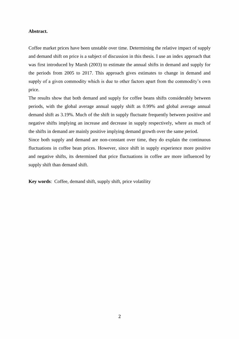
Abstract.

Coffee market prices have been unstable over time. Determining the relative impact of supply

and demand shift on price is a subject of discussion in this thesis. I use an index approach that

was first introduced by Marsh (2003) to estimate the annual shifts in demand and supply for

the periods from 2005 to 2017. This approach gives estimates to change in demand and

supply of a given commodity which is due to other factors apart from the commodity’s own

price.

The results show that both demand and supply for coffee beans shifts considerably between

periods, with the global average annual supply shift as 0.99% and global average annual

demand shift as 3.19%. Much of the shift in supply fluctuate frequently between positive and

negative shifts implying an increase and decrease in supply respectively, where as much of

the shifts in demand are mainly positive implying demand growth over the same period.

Since both supply and demand are non-constant over time, they do explain the continuous

fluctuations in coffee bean prices. However, since shift in supply experience more positive

and negative shifts, its determined that price fluctuations in coffee are more influenced by

supply shift than demand shift.

Key words: Coffee, demand shift, supply shift, price volatility

3

Table of Content:

Acknowledgement …………………………………………………………………………….1

Abstract ………………………………………………………………………………………. 2

List of figures and tables ………………………………………………………………………5

Chapter 1: Introduction ..………………………………………………………………… 6

1.1 Introduction …………………………………………………………………………… 6

1.2 Problem Statement ……………………………………………………………………. 7

1.3 Research questions ………………………………………………………………….... 8

Chapter 2: Literature Review ………………………………………………………………10

2.1 Demand and/or Supply ……………………………………………………………...10

2.2 Back ground to the study of demand and supply ……………………………………11

2.3 World coffee production and market situation ……………………………………...12

2.3.1 World demand ………………………………………………………………...12

2.3.2 World coffee supply and market …………………………………………...…14

2.3.3 Arabicas Vs Robustas ……………………………………………………….16

2.3.4 Current production by region ………………………………………………...18

2.4 The International Coffee Agreement (ICA) …………………………………………….19

Chapter 3: Method and Data ……………………………………………………………….22

3.1 Methodology for demand shift ……………………………………………………...22

3.2 Methodology for supply shift ……………………………………………………….27

3.3 Methodology for price determination ……………………………………………….29

3.4 Data …………………………………………………………………………………29

3.4.1 Quantity data …………………………. …………………………………….29

3.4.2 Price data …………………………………………………………………….30

3.4.3 Elasticity parameters.………………………………………………………...31

Chapter 4: Results and Discussions…………………………………………………………33

4.1 Introduction …………………………………………………………………………33

4.2 Results ……………………………………………………………………………....33

4.3 Discussions ……………………………....................................................................36

4.4 Sensitivity analysis ………………………………………………………………….39

Chapter 5: Summary and Conclusion ………………………………………………………41

4

5.1 Summary ……………………………………………………………………………41

5.2 Conclusions ………………………………………………………………………....42

References ……………………………………………………………………. 43

Appendix ……………………………………………………………………… 46

5

Figures and Tables.

List of figures

Figure 1: Quarterly world coffee prices ……………………………………………………….7

Figure 2: Coffee producing countries by type and region …………………………………...15

Figure 3: Coffee production by region ……………………………………………………….19

Figure 4: Horizontal shift in demand between two periods ………………………………….23

Figure 5: Vertical shift in demand …………………………………………………………...26

Figure 6: Horizontal supply and demand shift, impact on prices ……………………………27

List of Tables

Table 1: Summary statistics of price and quantity data ……………………………………...31

Table 2: Elasticity parameters’ summary statistics ………………………………………….32

Table 3: Relative changes in quantities and price ……………………………………………34

Table 4: Supply and Demand shifts, 2005-2017 …………………………………………….35

Table 5: Supply and Demand growth index, 2005=100 ………………………………….….38

Table 6: New annual average supply shifts ……………………………………………….…39

Table 7: New annual average demand shifts ………………………………………………...40

6

Chapter 1: Introduction

1.1 Introduction.

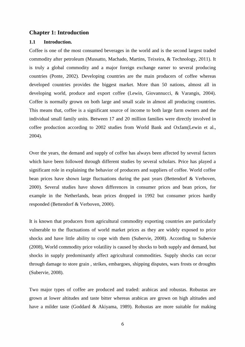
Coffee is one of the most consumed beverages in the world and is the second largest traded

commodity after petroleum (Mussatto, Machado, Martins, Teixeira, & Technology, 2011). It

is truly a global commodity and a major foreign exchange earner to several producing

countries (Ponte, 2002). Developing countries are the main producers of coffee whereas

developed countries provides the biggest market. More than 50 nations, almost all in

developing world, produce and export coffee (Lewin, Giovannucci, & Varangis, 2004).

Coffee is normally grown on both large and small scale in almost all producing countries.

This means that, coffee is a significant source of income to both large farm owners and the

individual small family units. Between 17 and 20 million families were directly involved in

coffee production according to 2002 studies from World Bank and Oxfam(Lewin et al.,

2004).

Over the years, the demand and supply of coffee has always been affected by several factors

which have been followed through different studies by several scholars. Price has played a

significant role in explaining the behavior of producers and suppliers of coffee. World coffee

bean prices have shown large fluctuations during the past years (Bettendorf & Verboven,

2000). Several studies have shown differences in consumer prices and bean prices, for

example in the Netherlands, bean prices dropped in 1992 but consumer prices hardly

responded (Bettendorf & Verboven, 2000).

It is known that producers from agricultural commodity exporting countries are particularly

vulnerable to the fluctuations of world market prices as they are widely exposed to price

shocks and have little ability to cope with them (Subervie, 2008). According to Subervie

(2008), World commodity price volatility is caused by shocks to both supply and demand, but

shocks in supply predominantly affect agricultural commodities. Supply shocks can occur

through damage to store grain , strikes, embargoes, shipping disputes, wars frosts or droughts

(Subervie, 2008).

Two major types of coffee are produced and traded: arabicas and robustas. Robustas are

grown at lower altitudes and taste bitter whereas arabicas are grown on high altitudes and

have a milder taste (Goddard & Akiyama, 1989). Robustas are more suitable for making

7

instant coffee as they produce a higher volume for a unit weight of beans. On average, arabica

prices are 10% higher than Robusta prices (Goddard & Akiyama, 1989).

In several coffee producing countries, coffee accounts for at least 20 percent of the total

export earnings, where approximately 100 million people are affected directly by the coffee

trade (Lewin et al., 2004). Therefore, changes in demand, supply and price of coffee would

destabilize the economies of the producing countries and the world market as well.

However, the prices of coffee have been fluctuating over time. These price volatilities have

had several consequences in different producing countries. The consequences of the crisis in

each country and region have been different according to the industry structure of the country

concerned.

1.2 Problem Statement.

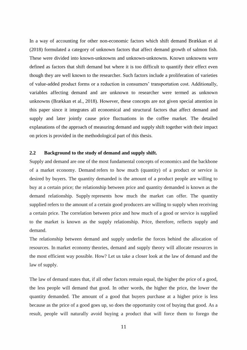
Price volatility in coffee has been a common occurrence in the industry for a long time, as it is

the case to most markets for agricultural commodities (Tomek & Robinson, 2003). In general,

agricultural produce are characterized with a combination of short periods of high and volatile

prices and long periods of low prices and low volatility (Deaton & Laroque, 1992). Therefore,

price instabilities in agricultural commodities, coffee inclusive are inevitable. Over the period

since 1970s, prices have averaged a 3 percent per year price decline for arabica and a 5

percent decline for Robusta (Lewin et al., 2004).

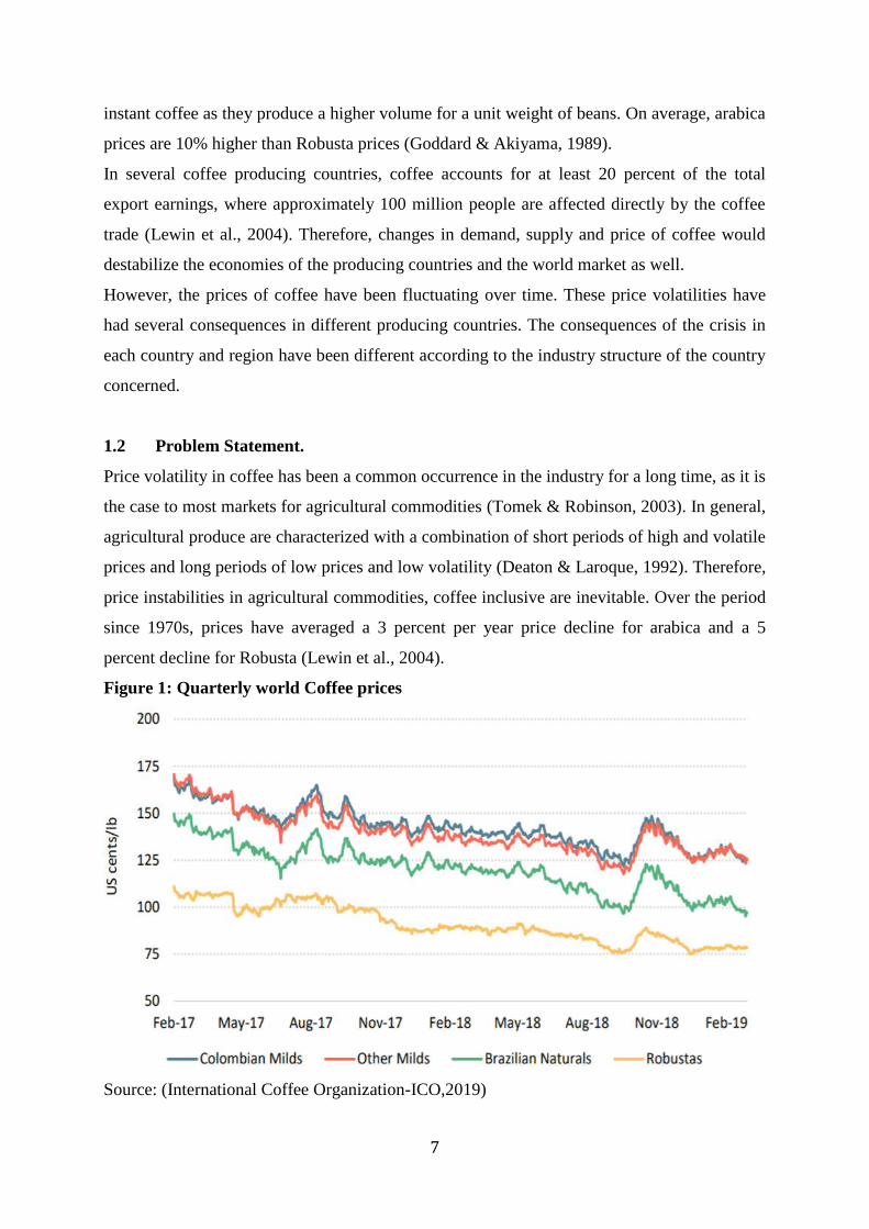
Figure 1: Quarterly world Coffee prices

Source: (International Coffee Organization-ICO,2019)

8

The falling trend in prices was characterized by among others the combination of increased

productivity, rising production as new lower-cost producers enter the market , rising share of

export prices, and a sequence of renewable planting and innovation that follows price spikes

that occur occasionally, usually following a frost or drought in Brazil (Lewin et al., 2004).

As in the market of other agricultural commodities, long spells of declines in coffee prices are

followed with short spells of increase in prices. This could also be attributed to several factors

such as farmers’ speculations. Once excess supply is in the system and prices have fallen,

these stocks act as a restraint on price increases coming from a short-run supply fluctuations

because traders will hold stocks for both speculative reasons, expecting to sell them for a

profit at a later date if price rise, and for precautionary reasons expecting to meet sales

obligations to roasters during shorter periods of coffee unavailability (Lewin et al., 2004)

In figure 1 above, price for all forms of coffee beans are represented and the patterns shows

quarterly fluctuations according to ICO (2019) for most recent records. Robusta’s prices are

relatively lower than all Arabica coffee types, nevertheless none of the coffee types exhibits

constant price trends over time.

The exogenous factors that shift demand and supply contributes to unexplained changes in

price of agricultural and perishable commodities. Therefore, this thesis studies the way prices

fluctuations in the global coffee market has been influenced by un explained changes in

demand and/ or supply. Prices can increase due to increased demand or reduced supply.

Demand and supply factors can also simultaneously contribute to changes in food prices

(Trostle, 2010).

1.3 Research question.

As coffee is one of the most foreign exchange earners for majority of the producing

developing countries, it’s also a source of consumer satisfaction both to importing and

producing countries. Therefore, understating the growth in demand and supply for coffee and

their impact on price is a global concern hence a point of concentration in this thesis. In this

regard the following questions have been formulated as a basis for this research:

1. What is the level and nature of demand growth for coffee in the world market over a

given period?

2. What is the level and nature of supply growth of coffee in the world market over a

given period?

3. What is the impact of demand and supply shifts on coffee price volatility in the world

market?

9

The concept of demand shifters and supply shifters is applied to understand the level and the

nature of growth in accordance to the given research questions. In this case the nature can be a

positive shift, a negative shift or a combination of the two. The Level of growth is a

percentage at which a given variable has changed or shifted from one period to another.

When either demand or supply for a given commodity shifts, future prices are affected. This

research therefore concludes by determining if really shifts are experienced in the coffee

market to know the reason behind substantial unstable coffee prices in the world market.

10

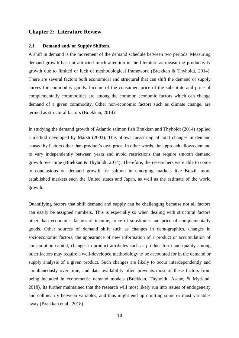
Chapter 2: Literature Review.

2.1 Demand and/ or Supply Shifters.

A shift in demand is the movement of the demand schedule between two periods. Measuring

demand growth has not attracted much attention in the literature as measuring productivity

growth due to limited or luck of methodological framework (Brækkan & Thyholdt, 2014).

There are several factors both economical and structural that can shift the demand or supply

curves for commodity goods. Income of the consumer, price of the substitute and price of

complementally commodities are among the common economic factors which can change

demand of a given commodity. Other non-economic factors such as climate change, are

termed as structural factors (Brækkan, 2014).

In studying the demand growth of Atlantic salmon fish Brækkan and Thyholdt (2014) applied

a method developed by Marsh (2003). This allows measuring of total changes in demand

caused by factors other than product’s own price. In other words, the approach allows demand

to vary independently between years and avoid restrictions that require smooth demand

growth over time (Brækkan & Thyholdt, 2014). Therefore, the researchers were able to come

to conclusions on demand growth for salmon in emerging markets like Brazil, more

established markets such the United states and Japan, as well as the estimate of the world

growth.

Quantifying factors that shift demand and supply can be challenging because not all factors

can easily be assigned numbers. This is especially so when dealing with structural factors

other than economics factors of income, price of substitutes and price of complementally

goods. Other sources of demand shift such as changes in demographics, changes in

socioeconomic factors, the appearance of new information of a product or accumulation of

consumption capital, changes in product attributes such as product form and quality among

other factors may require a well-developed methodology to be accounted for in the demand or

supply analysis of a given product. Such changes are likely to occur interdependently and

simultaneously over time, and data availability often prevents most of these factors from

being included in econometric demand models (Brækkan, Thyholdt, Asche, & Myrland,

2018). Its further maintained that the research will most likely run into issues of endogeneity

and collinearity between variables, and thus might end up omitting some or most variables

away (Brækkan et al., 2018).

11

In a way of accounting for other non-economic factors which shift demand Brækkan et al

(2018) formulated a category of unknown factors that affect demand growth of salmon fish.

These were divided into known-unknowns and unknown-unknowns. Known unknowns were

defined as factors that shift demand but where it is too difficult to quantify their effect even

though they are well known to the researcher. Such factors include a proliferation of varieties

of value-added product forms or a reduction in consumers’ transportation cost. Additionally,

variables affecting demand and are unknown to researcher were termed as unknown

unknowns (Brækkan et al., 2018). However, these concepts are not given special attention in

this paper since it integrates all economical and structural factors that affect demand and

supply and later jointly cause price fluctuations in the coffee market. The detailed

explanations of the approach of measuring demand and supply shift together with their impact

on prices is provided in the methodological part of this thesis.

2.2 Background to the study of demand and supply shift.

Supply and demand are one of the most fundamental concepts of economics and the backbone

of a market economy. Demand refers to how much (quantity) of a product or service is

desired by buyers. The quantity demanded is the amount of a product people are willing to

buy at a certain price; the relationship between price and quantity demanded is known as the

demand relationship. Supply represents how much the market can offer. The quantity

supplied refers to the amount of a certain good producers are willing to supply when receiving

a certain price. The correlation between price and how much of a good or service is supplied

to the market is known as the supply relationship. Price, therefore, reflects supply and

demand.

The relationship between demand and supply underlie the forces behind the allocation of

resources. In market economy theories, demand and supply theory will allocate resources in

the most efficient way possible. How? Let us take a closer look at the law of demand and the

law of supply.

The law of demand states that, if all other factors remain equal, the higher the price of a good,

the less people will demand that good. In other words, the higher the price, the lower the

quantity demanded. The amount of a good that buyers purchase at a higher price is less

because as the price of a good goes up, so does the opportunity cost of buying that good. As a

result, people will naturally avoid buying a product that will force them to forego the

12

consumption of something else they value more. The general principle of the law of demand

was introduced by Marshall in the 1920s (Marshall, 1961). Like the law of demand, the law of

supply demonstrates the quantities that will be sold at a certain price (A. Smith, 1863). But

unlike the law of demand, the supply relationship shows an upward slope. This means that the

higher the price, the higher the quantity supplied. Producers supply more at a higher price

because selling a higher quantity at a higher price increases revenue.

Demand shift and supply shift however assumes a constant commodity price. In other words,

these variables can increase or decrease in response to other factors other than commodity’s

own price. In chapter 3, graphical explanations and equations are provided to give a broad

picture on the differences between change in quantity demanded or supplied and change in

demand or supply (demand shift and supply shift for this case).

In accordance to Brækkan (2014), the true nature of demand and supply curves caused a

controversy among economists. In what was termed as the notorious “pitfalls debate” between

Frisch (1933) and Leontief (1929), the former violently disagrees when the later derived a

procedure for estimating supply and demand curves by using only price and quantity data

based on independence of demand and supply principle (Brækkan, 2014). Frisch stated that

the nature of the specific data would contradict the underlying assumption of independence

between shifts in supply and demand. Brækkan (2014) further notes that the disagreement

reflects two fundamental approaches to demand and supply analysis; in one the economic

theory of supply and demand comprises the essential foundation for useful data analysis; in

the other, the data at hand be taken into consideration in any analytical approach. Therefore,

Leontief was considered a strong proponent of the use of quantitative data in estimating

demand and supply whereas Frisch is considered the founder of econometrics (Brækkan,

2014).

2.3 World Coffee production and Market Situation

2.3.1 World demand.

World demand for coffee in 2003 was approximately 115 million bags, comprised of about 87

million bags in importing countries and 28 million bags in producing countries (Lewin et al.,

2004). Additionally, 65 percent of the world’s coffee was consumed by just 17 percent of the

world’s population before 2004 which indicates opportunities for market growth.

13

From continental perspective, European countries consumed the highest dollar worth of

imported coffee during 2018 with purchases valued at US dollars (USD) 18.2 billion or

58.8% of the global total. In second place were North American importers at 22.6% while

13.6% of coffee imports were delivered to Asia. Africa and Oceania imported nearly the same

amount that accounted for 1.8% each. Much of the Oceania’s imports is dominated by

Australia and New Zealand, and then Latin America imported 1.3% excluding Mexico but

including the Caribbean (Daniel, 2019). It is clearly not a surprise that Asia, Africa and South

America imports the least amount of coffee since they are the major producing regions.

Therefore, although much of their produce is exported, they also reserve a proportion to be

consumed in their domestic markets.

The United states is one of the world’s largest coffee importers, they import from a variety of

different countries, which are aggregated into different groups representing a certain number

of broadly defined types of coffee (Goddard & Akiyama, 1989). In the year 1964-1982, the

United states of America remained the world’s largest importer and it imported between 27

and 45 percent of total worlds imports. According to Akiyama (1969), the United states of

America re-exported only a small percentage of its coffee imports of about 7 percent and the

rest was observed in domestic consumption. Like in most countries, coffee consumption in

the United States of America is affected by the structure of the population. Immediately after

the postwar period, the income elasticity of coffee was negative for small children and youth

and positive for the elderly (Hughes, 1969). In other words, coffee becomes an inferior good

as one gets younger and, in most cases, a normal good for the elderly. Therefore, a change in

the population structure can be another factor the results into substantial shift in demand for

coffee in a given economy

In Sweden, there is a wide spread belief that consumer coffee prices are high relative to bean

prices and that lower consumer prices would lead to substantial increase in bean export from

third world countries (Durevall, 2007). A low-price elasticity of demand for coffee in Sweden

was established at 0.19 for the period between 1968 and 2002, and it was determined that

impact of price decrease would be small because of the long-run coffee demand is dominated

by changes in the population structure in combination with different preferences across age

group

14

2.3.2 world coffee supply and market.

As earlier mentioned, coffee is mainly produced by world’s developing countries especially in

South America, Asia and Africa. Brazil, Colombia and Vietnam are the major producers. In

accordance to United States Department of Agriculture (USDA), it was estimated that world

production has been rising by an average of 1.8 percent per year since 1965, which was a

consistent increase despite the decrease in real prices (Lewin et al., 2004). The growth rate

drops to 1.4 percent when these three producing countries are removed from the picture

implying that the most recent growth of the world supply came from the first two of these

origins.

In the periods between the year 1960 and 2003, production from Latin America was the

highest followed by Africa. However, Asia experienced an increasing trend and Africa

exhibited a relatively constant and later a decreasing trend in gross production. Therefore,

towards the late 1990s, total production from Asia surpassed total production in Africa.

Brazil and other countries in the Central South America are the major producers of Arabica

coffee while majority of African and Asian countries are the major producers of Robusta. The

International Coffee Agreement (ICA) divides coffee output into four major groups. These

include two groups for washed arabicas, and one group each for natural arabicas and robustas.

Additionally, the washed arabica group is divided in two as Colombian Milds and Other

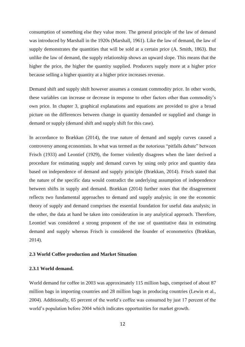
Milds. The following table shows Fifty-five producing countries by principal type and region.

15

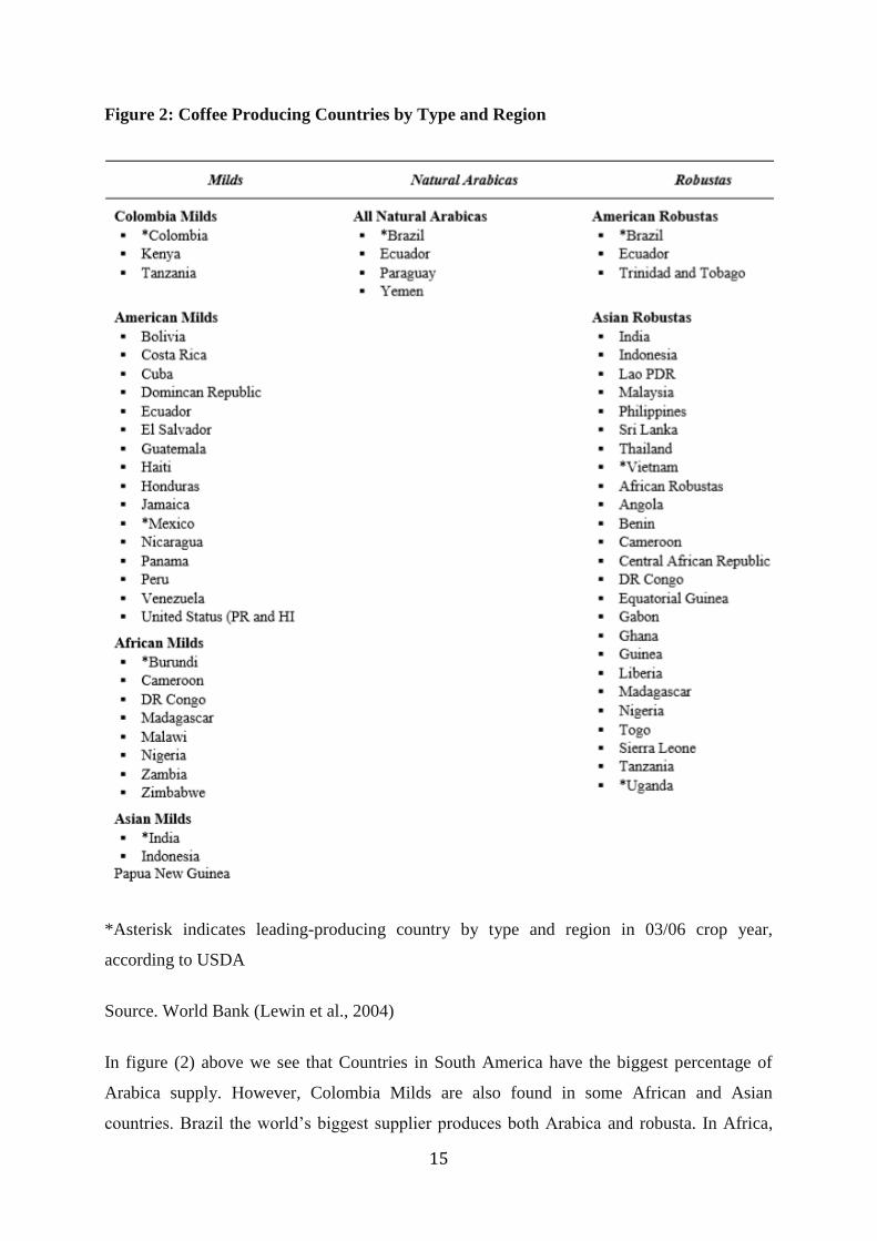
Figure 2: Coffee Producing Countries by Type and Region

*Asterisk indicates leading-producing country by type and region in 03/06 crop year,

according to USDA

Source. World Bank (Lewin et al., 2004)

In figure (2) above we see that Countries in South America have the biggest percentage of

Arabica supply. However, Colombia Milds are also found in some African and Asian

countries. Brazil the world’s biggest supplier produces both Arabica and robusta. In Africa,

16

Uganda is a major supplier of Robusta despite the changing quantity levels. Below is a

detailed explanation of the major coffee types, their sub categories and their place of

production.

2.3.3 Arabicas vs Robatas.

Arabicas

Arabica contributes about 70 percent of total production in the world (Bunn, Läderach,

Rivera, & Kirschke, 2015). It is a type of coffee made from the beans of the coffee arabica

plant. Arabica coffee is said to have originated in southwestern highlands of Ethiopia where it

was eaten as stimulant by the Oromo tribe. Furthermore, It went to Arabia in the 7th century

where it was said to have been born, hence the name “Arabica coffee” (Dena, 2018).

In accordance to figure (2), Arabica is categorized into natural and Colombian Milds. Natural

Arabica is unwashed arabica, where the production process does not involve water. The

cherries are dried in the sun or in mechanical dryers and then milled to produce green beans.

The two biggest producers of Natural Arabica are Brazil and Ethiopia (Lewin et al., 2004).

The quality of natural arabica is substantially high due absence of water contacts which would

affect the produce during fermentation of water and the cherry. Lewin et al (2014) notes that

both Brazil and Ethiopia produce some washed and (in Brazil) semi-washed coffee.

Therefore, Brazilian arabica have a major impact on the world’s coffee market given both the

country’s total volume and the willingness of the industry to use them to replace other

arabicas in their blends according to price.

Washed Arabicas is another category of arabica as shown in figure (2), which is also

separated into Colombian Milds (mostly for Colombia) and other Milds (mostly for

American, African and Asian). Colombia and Kenya are among the major producers of

Colombian Milds. In the two countries, the cost of production is quite high due to the efforts

made to maintain the quality of the output. Colombia alone is the world’s largest producer of

washed arabica and the world’s second largest producer of coffee in general (Lewin et al.,

2004). A series of Unique circumstances including fertilizers subsidies in the early 1990s

briefly pushed production to reach a record high of 18 million bags in early 2000s (Lewin et

al., 2004). Despite the shirking production area, Colombia’s increased productivity per

17

hectare is an important factor in its ability to control quality and costs, still according to

Lewin (2004).

The two East African Countries of Kenya and the United Republic of Tanzania both produce

some of the world’s finest washed arabicas, although the United Republic of Tanzania

produces both arabica and Robusta (Lewin et al., 2004).

“Other Milds category” involves all washed arabicas from other producing countries other

than Colombia. These include American Milds, Asian Milds and African Milds. In Latin

America, Central American production peaked at 21.3 million bags in 1990-2000, which later

experienced some shifts with countries such as El Salvador and Panama, unable to sustain

their periodic advances, making production to fall for three consecutive years because of low

prices between 2000 and 2003 (Lewin et al., 2004). In 1993 Peru became a significant washed

arabica producer whose production rose to nearly 3 million bags during the same crop year.

According to Lewin (2004), the production growth came because of two sets of influences:

First, higher coffee prices following the Brazil frost led economic incentives to shift illicit

crops, and this was aided at the same time by a steep drop in the price of some illicit drug

crops following successful action by the Colombian government that broke the supply chain

for these products. The second set of influence was a combination of internal political and

economic liberalization, as well as a partial settlement of the security situation that allowed

farmers access to land that gave them confidence in expanding production. Venezuela,

Ecuador and Bolivia also produce washed arabica with Ecuador producing both washed and

unwashed Arabica. The quantities from these countries are relatively lower due to political

instabilities, poor infrastructure and other structural factors according to Lewin (2004).

Robustas.

Robusta accounts to almost 30 percent of the total world coffee production, with Vietnam and

Brazil as the biggest producers (Lewin et al., 2004). Robusta is noted for its resistance to

diseases hence suitable for growth in tropical environments of Africa which are most

vulnerable to pests and diseases (Van der Vossen, 2009). Although Robusta coffee has a

flavor that is inferior to that of arabica coffee, with a caffeine content more than double , it

has in proportion a greater stimulating action, and also offered advantages to the

manufacturers of instant coffee extracts, and also has a higher content soluble extractives

which makes it more economical in the manufacturers of instant coffee (R. F. Smith, 1985).

18

Vietnam is by far the main producer after Brazil but Ivory Coast, Indonesia and Uganda are

also major players (Ponte, 2002). In accordance to figure (2) Robustas is categorized

according to the place of origin, which clearly shows that there are more Asian and African

producing countries than Latin America robustas producers.

In Asia Vietnam’s Robusta production grew at an average rate of about 27 percent per year in

early 2000s making it the second largest producer of Robusta after Brazil and the world’s

third largest producer of coffee in general after Brazil and Colombia. According to Lewin

(2004) Brazil and Vietnam together added 20 million bags to the world supply since 1991.In

Africa, Robusta production is dominated by two main producers Ivory Coast which produces

only Robusta and Uganda of which 90 percent is Robusta (Lewin et al., 2004).

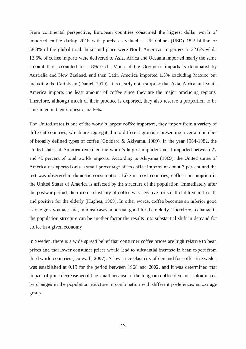
2.3.4 Current World production by Region

Currently, South America is by far the largest producer due to the presence of Brazil and

Colombia which are world giants in production of both arabica and robusta coffee. According

to International Coffee Organization (ICO), Brazil’s production in coffee year 2018/19,

amounted to a record 60.1million bags, which has contributed to oversupply of coffee in this

crop year, and Colombia is estimated to have harvested 14.2 million bags, an increase of 2.7%

compared to the previous year 2017/18 (ICO, 2019). Asia and Oceania take the second step,

Central America and Mexico in the third place and Africa the least place, as shown by figure

(3) below:

19

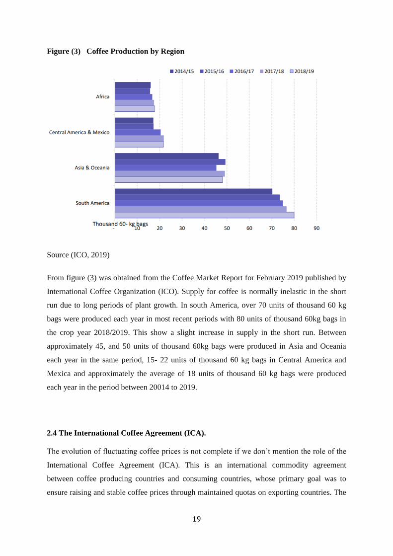
Figure (3) Coffee Production by Region

Source (ICO, 2019)

From figure (3) was obtained from the Coffee Market Report for February 2019 published by

International Coffee Organization (ICO). Supply for coffee is normally inelastic in the short

run due to long periods of plant growth. In south America, over 70 units of thousand 60 kg

bags were produced each year in most recent periods with 80 units of thousand 60kg bags in

the crop year 2018/2019. This show a slight increase in supply in the short run. Between

approximately 45, and 50 units of thousand 60kg bags were produced in Asia and Oceania

each year in the same period, 15- 22 units of thousand 60 kg bags in Central America and

Mexica and approximately the average of 18 units of thousand 60 kg bags were produced

each year in the period between 20014 to 2019.

2.4 The International Coffee Agreement (ICA).

The evolution of fluctuating coffee prices is not complete if we don’t mention the role of the

International Coffee Agreement (ICA). This is an international commodity agreement

between coffee producing countries and consuming countries, whose primary goal was to

ensure raising and stable coffee prices through maintained quotas on exporting countries. The

20

agreement was signed in 1962 (Mehta & Chavas, 2008) for the first time, and later it

temporarily collapsed in 1989 (Charveriat, Practice: Agriculture, & Land, 2001).The ICA

evolved from the Inter-American Coffee Agreement (IACA) signed in 1940 between the

United States and fourteen Latin-American coffee producing countries, which was aimed to

lessen the burden imposed by the loss of European market to Latin American producers

(Pichop & Kemegue, 2005). Following the signing of IACA, the United states restricted its

importing quotas to a certain amount and the Latin American countries restricted their

production, which doubled the prices by the end of 1940. Prices increased continuously until

the attainment of degree of equilibrium in 1957.

An attempt to maintain the price, gave way to the signing of the first ICA, where a target price

was set, and export quotas were allocated to each producing country. The requirements of the

agreement were supervised by the International Coffee Organization (ICO). According to

Pichop and Kemegue (2005), members mutually agreed to stabilize prices by increasing

consumption, achieve a long- term equilibrium between production and consumption and

assure adequate supply to consumers and markets to producers at equitable prices. In

stabilizing market prices, ICO increased quotas when price rose above the set price, and the

quotas were decreased whenever prices fell below the set price (Daviron & Ponte, 2005).

During the operation of the ICA, two coffee markets co-existed with one involving consumers

from member countries and the other involving consumers in non-member countries.

Therefore, the imposition of the world quota caused prices in member market to rise above

the free trade price, and prices in the nonmember market to fall below the level, according to

Pichop and Kemegue (2005). So Coffee exporters thus faced two distinct markets: one with

high prices constrained by quotas and the other unconstrained with low prices, a situation

which was earlier predicted (Mikesell, 1963).

In 1983, new quotas were instituted on each producer, which brought about some

disagreements among the member states. The changing consumer tastes in favor of milder and

high-quality coffee (Daviron & Ponte, 2005), led to major producers especially Brazil not to

comply to new quotas set. Brazil for example failed to reduce its quotas despite its falling

market share. This, together with the dissatisfaction among importing member countries

stemmed from the lower prices paid by nonmember countries led to failure of the ICA in

1989. Free markets were therefore established and the agreement became a mere statement of

good intentions from member states (Pichop & Kemegue, 2005).

21

The most recent agreement is the International Coffee Agreement 2007, the seventh since

1962. This is agreed by exporting and importing countries, where the European Union (EU) is

taken as on importing country to represent 28 individual countries.

Unlike the previous agreements, “ the 2007 agreement will strengthen the ICO’s role as the

forum for intergovernmental consultations, facilitate international trade through increased

transparency and access to relevant information, promote a sustainable coffee economy for

the benefit of all stakeholders and particularly of small-scale farmers in coffee producing

countries”, (ICO, 2007)

22

Chapter 3 Method and Data

3.1 Methodology for demand shift

The approach used to measure shifts in demand and supply is based on works of Mash (2003),

where it was first introduced and later used by different researchers in agricultural and food

commodity economics. In the study about demand for beef in the United States, Marsh

defined shifts in the retail demand for beef as a percentage change difference between

observed retail beef prices and estimated retail prices holding demand constant (Marsh, 2003).

Demand shift as explained in Chapter 2 entails a movement of the demand schedule, the

inward and outward movement of the demand curve represents decrease and increase in

demand respectively. However, the movement can be either horizontally or vertically

(Wohlgenant & policy, 2011).

A horizontal shift can be interpreted as a change in quantity demanded at a given price while

a vertical shift can be interpreted as the change in consumers’ willingness to pay for a given

quantity (Brækkan et al., 2018). In this study for coffee, the demand shift in quantity direction

(horizontal) is chosen. It’s is also noted that when given Horizontal shift, the corresponding

vertical shift can simply be obtained (Sun & Kinnucan, 2001).

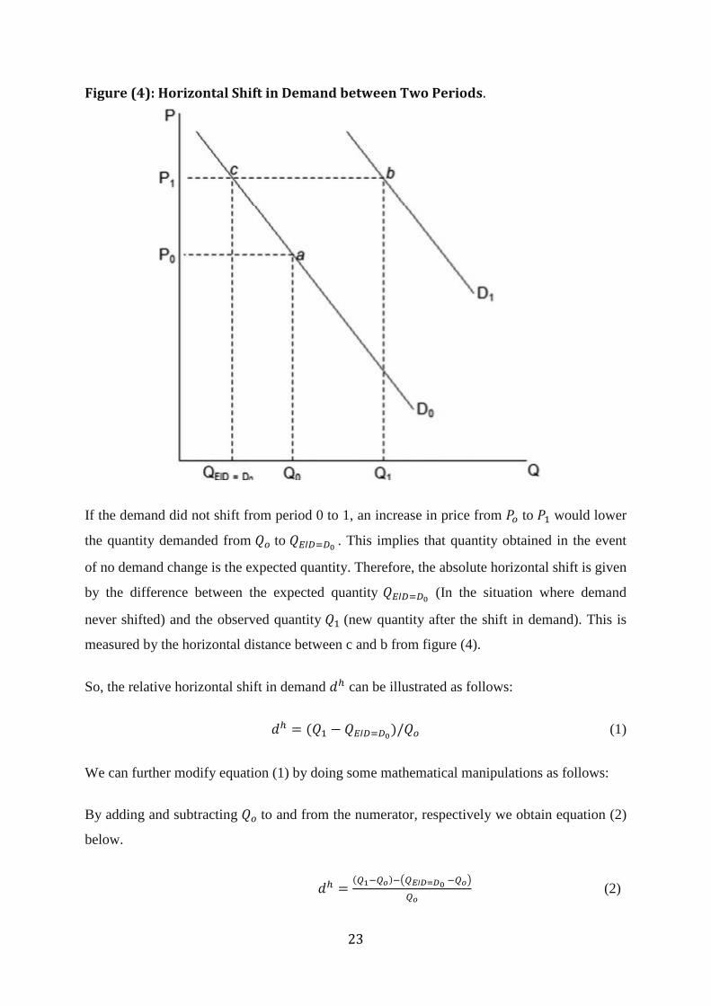
In figure (4) below, a shift in quantity direction is illustrated when demand is studied for two

periods 0 and 1. Each period is represented by its own demand schedule.

𝐷𝑜 is the demand schedule for period 0 and 𝐷1 is the demand schedule for period 1. 𝑃𝑜 and 𝑄𝑜

are equilibrium price and the quantity for periods 0, respectively. 𝑃1 and 𝑄1 are equilibrium

price and quantity in period 1, respectively.

23

Figure (4): Horizontal Shift in Demand between Two Periods.

If the demand did not shift from period 0 to 1, an increase in price from 𝑃𝑜 to 𝑃1 would lower

the quantity demanded from 𝑄𝑜 to 𝑄𝐸𝘐𝐷=𝐷0 . This implies that quantity obtained in the event

of no demand change is the expected quantity. Therefore, the absolute horizontal shift is given

by the difference between the expected quantity 𝑄𝐸𝘐𝐷=𝐷0 (In the situation where demand

never shifted) and the observed quantity 𝑄1 (new quantity after the shift in demand). This is

measured by the horizontal distance between c and b from figure (4).

So, the relative horizontal shift in demand 𝑑ℎ can be illustrated as follows:

𝑑ℎ = (𝑄1 − 𝑄𝐸𝘐𝐷=𝐷0)/𝑄𝑜 (1)

We can further modify equation (1) by doing some mathematical manipulations as follows:

By adding and subtracting 𝑄𝑜 to and from the numerator, respectively we obtain equation (2)

below.

𝑑ℎ =(𝑄1−𝑄𝑜)−(𝑄𝐸𝘐𝐷=𝐷0 −𝑄𝑜)

𝑄𝑜 (2)

24

Equation (2) shows the difference between the actual and the expected relative change in

quantity where, (𝑄1 − 𝑄𝑜)/𝑄𝑜 = 𝑄∗is the observed relative change in quantity,

and (𝑄𝐸𝘐𝐷=𝐷0 −𝑄𝑜)

𝑄𝑜= 𝑄𝐸

∗ is the relative difference between expected quantity in period 1 and

observed quantity in period zero.

Now we must determine the value of 𝑄𝐸∗ by using the common definition of the price

elasticity of demand (η)

η =percentage change in quantity

percentage change in price

η =

Q1−𝑄0𝑄𝑜

𝑃1−𝑃𝑜

𝑃𝑜 (3)

In this case, we must use the expected quantity 𝑄𝐸𝘐𝐷=𝐷0 in case of no demand shift instead of

𝑄1, which gives the following expression:

η =

Q𝐸𝘐𝐷=𝐷0−𝑄0

𝑄𝑜𝑃1−𝑃𝑜

𝑃𝑜 (4)

Simplifying of the equation (4) by doing cross multiplication we obtain the following

expression:

(𝑄𝐸𝘐𝐷=𝐷0 −𝑄𝑜)

𝑄𝑜=

η(P1−𝑃𝑜)

𝑃𝑜 (5)

From equation (5) the expression of the Left-Hand Side (LHS) is equal to the expected

relative change in quantity 𝑄𝐸∗ . In accordance with the demand schedule, 𝐷𝑜, the price change

corresponding to 𝑄𝐸∗ is the relative price change,

𝑃1−𝑃0

𝑃𝑂= 𝑃∗ , on the Right-Hand Side (RHS)

of the equation (5).

25

This follows that if given the change in price, 𝑃∗ and the predetermined elasticity of demand

η,we can solve equation (5) for the relative change in quantity 𝑄𝐸∗ . Therefore, equating the

LHS to the RHS of equation (5) we obtain the following expression:

𝑄𝐸∗ = ηP∗ (6)

By substituting for 𝑄𝐸∗ from equation (6) into equation (2), the relative shift in demand can be

obtained as follows.

𝑑ℎ = 𝑄∗ − ηP∗ (7)

Alternatively, we define the expected relative change in quantity as follows

𝑄∗ = 𝑑ℎ + ηP∗ (8)

The asterisks (*) denotes relative change throughout this study. In other words, relative

changes for the commodity in question “coffee” with regards to price and expected quantity

will be obtained in the subsequent chapter.

In addition, the elasticities from the previous research will be used to cater for the values of η

as shown in chapter 4 of the analysis section.

Figure (4), Illustrates horizontal shifts in demand 𝑑ℎ which is mathematically obtained in

equation (7). When given the horizontal shift in demand, the corresponding vertical shift can

be obtained dividing by the negative elasticity of demand (Sun & Kinnucan, 2001). Hence the

expression for demand shift from the price side is obtained in equation (9) below:

𝑑𝑣 =𝑑ℎ

− η (9)

The argument for vertical shift in demand is not different from that of the horizontal shift in

demand. The only unique aspect is that the during vertical shift in demand, the expected price

level 𝑃𝐸𝘐𝐷=𝐷0 is determined at a point in case demand is assumed not to have shifted as

illustrated by figure (5) below.

26

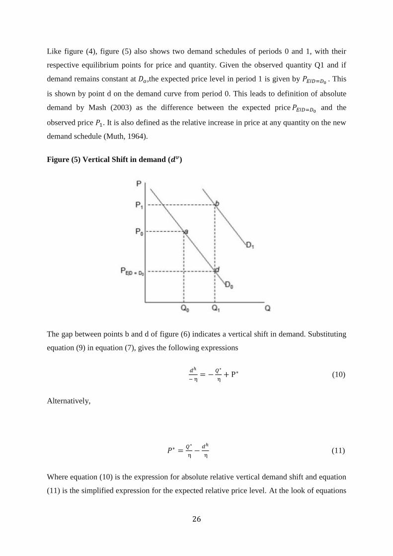
Like figure (4), figure (5) also shows two demand schedules of periods 0 and 1, with their

respective equilibrium points for price and quantity. Given the observed quantity Q1 and if

demand remains constant at 𝐷𝑜,the expected price level in period 1 is given by 𝑃𝐸𝘐𝐷=𝐷0 . This

is shown by point d on the demand curve from period 0. This leads to definition of absolute

demand by Mash (2003) as the difference between the expected price 𝑃𝐸𝘐𝐷=𝐷0 and the

observed price 𝑃1. It is also defined as the relative increase in price at any quantity on the new

demand schedule (Muth, 1964).

Figure (5) Vertical Shift in demand (𝒅𝒗)

The gap between points b and d of figure (6) indicates a vertical shift in demand. Substituting

equation (9) in equation (7), gives the following expressions

𝑑ℎ

− η= −

𝑄∗

η+ P∗ (10)

Alternatively,

𝑃∗ =𝑄∗

η−

𝑑ℎ

η (11)

Where equation (10) is the expression for absolute relative vertical demand shift and equation

(11) is the simplified expression for the expected relative price level. At the look of equations

27

(10), the vertical demand shift is identical to horizontal demand shift if the elasticity of

demand is -1.

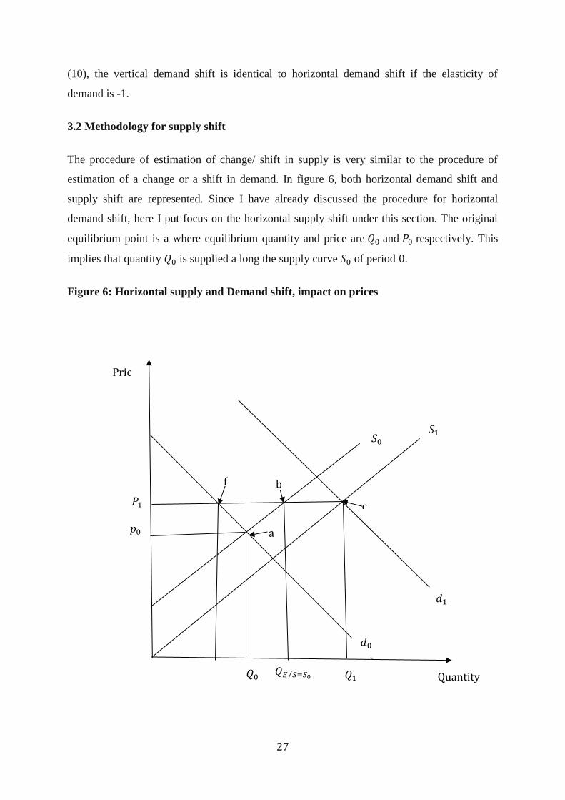
3.2 Methodology for supply shift

The procedure of estimation of change/ shift in supply is very similar to the procedure of

estimation of a change or a shift in demand. In figure 6, both horizontal demand shift and

supply shift are represented. Since I have already discussed the procedure for horizontal

demand shift, here I put focus on the horizontal supply shift under this section. The original

equilibrium point is a where equilibrium quantity and price are 𝑄0 and 𝑃0 respectively. This

implies that quantity 𝑄0 is supplied a long the supply curve 𝑆0 of period 0.

Figure 6: Horizontal supply and Demand shift, impact on prices

Price

𝑆0 𝑆1

𝑑0

𝑑1

𝑄1 𝑄𝐸 𝑆⁄ =𝑆0 𝑄0

𝑝0

𝑃1

b

c

f

a

Quantity

28

An increase in supply from period between period 0 and 1 can change the equilibrium to

point c if the outward shift of the supply curve from 𝑆0 to 𝑆1is accompanied by the demand

shift as shown by curve 𝑑0to 𝑑1. This will lead to equilibrium quantity 𝑄1.However, if only

demand changed in period 1 and supply curve never shifted, 𝑄𝐸𝘐𝑆=𝑆0 would have been the

new quantity supplied at a higher new price 𝑝1.

In this case the observed quantity for period 1 is 𝑄1 and the expected quantity (in case of no

supply shift) is 𝑄𝐸𝘐𝑆=𝑆0 . The absolute shift in supply is defined as the horizontal difference

between the supply schedules in periods 0 and 1, which is equal to the horizontal distance

between points c and b in figure 6.

Following the same procedure as shift in demand from equation (1) to equation (7), we obtain

the following expression for horizontal shift in supply.

𝑆ℎ = 𝑄𝑠∗ − 𝜀𝑃∗ (12)

Where: 𝑆ℎ is the horizontal shift in supply of coffee.

𝜀 is the price elasticity of supply.

𝑃∗ is the relative change in price.

The vertical supply shift can be computed simply by dividing equation (12) by negative

elasticity of supply, hence expression below:

𝑆ℎ

− 𝜀 = −

QS∗

𝜀 + P∗ (13)

29

3.3 Methodology for price Determination

Under the Equilibrium Displacement Model (EDM), the forces of demand and supply

determines the equilibrium price. When demand curve shifts out words to represent a growth

in demand without a substantial growth in supply in the same period, consumers would

compete for the scarce commodity hence forcing producers to supply at higher prices. In the

same way a fall in demand will force suppliers to lower the prices to attract and encourage

buyers.

When supply increase (positive shift in supply), it may create excess supply in case demand

remained constant, hence forcing producers to sell at lower prices to encourage buyers to take

up their excess surplus in the market. A decrease in supply will create scarcity of a product,

hence selling the competitive scarce commodity at higher prices.

Therefore, whenever demand or supply shift, prices are directly affected and determined

within the EDM. If the outcome of the study represents continuous shifts in supply and

demand, it will automatically tell something about the continuous price fluctuation in the

coffee market.

3.4 Data

The international Coffee Organization (ICO) avails free data to download from 1990 to

present. The ICO is an intergovernmental organization established by the United Nations in

1962, including both coffees’ producing and consuming member countries (Osorio, 2002). It

specifically addresses world coffee problems and issues in view of coffee’s exceptional

economic importance and development implications.

I relation to the period 2005-2017, I was able to download the required quantities and prices.

All quantities are given in thousands of 60kg bags and prices are in US cents per pound.

3.4.1 Quantity Data

Quantity data gives the amount of coffee beans that are demanded and supplied. On supply

side, I consider data about total production by all exporting countries. According to ICO, all

exporting countries are categorized into five production seasons depending on when each

30

country harvests coffee beans. These periods include April, July and October. Additionally,

quantities for both Arabica and Robusta were given for each country that produce both.

However, this research is based on aggregation of all forms of coffee and all seasons of

harvest are treated as a one-year production period. Therefore, the final data set that

represented the supply for each year is a summation of all production in all countries. In this

regard, annual production totals in thousands of 60kg bags were obtained to represent

quantity supplied.

Import data is used to represent demand. Even though most producing countries have

domestic demand, more of their production totals is exported to the international market

(Balassa, 1990). Therefore, demand for coffee from most developing producing countries is

almost equivalent to the amount that is exported. ICO provides quantities imported by the

European Union, Japan, Russian Federation, Tunisia, USA and Switzerland. Tunisia is the

only African importing country represented and none from Asia. However much some

African and Asian countries import a given amount to supplement their domestic production,

their share on total imports in very small (Slob, Osterhaus, & Challenges of Fair Trade, 2006)

and it cannot influence the results of this study. Total quantity imported in thousands of 60kg

bags were for each year were obtained.

3.4.2 Price Data

ICO provides a variety of prices which includes price given to growers, retail prices and ICO

Composite indicator prices. I chose to use ICO composite price indicator for simplicity. This

is the annual average ICO obtained from group indicator prices. According to ICO (2019)

group indicator prices are prices to all forms of coffee which include Colombian milds, Other

milds, Brazilian naturals and Robusta. In the same coffee market, prices of all forms of coffee

are cointegrated, hence forming the ICO composite indicator price that is a representative of

all forms of coffee prices

The nature of ICO composite price indicator is also supported by other studies that tested co-

integration among various types of coffee. Ghoshray (2010) found overwhelming support for

co-integration when non-linear Exponential Smooth Transition Autoregressive(ESTAR )

adjustment approach was used to test the prices of different coffee types (Ghoshray, 2010).

31

This therefore implies a single market and the average of all prices give reliable results

(R.Carter, William E, & Guay 2018), since a price change in a particular type of coffee would

lead to a similar change in the price of other quality of coffee in the market.

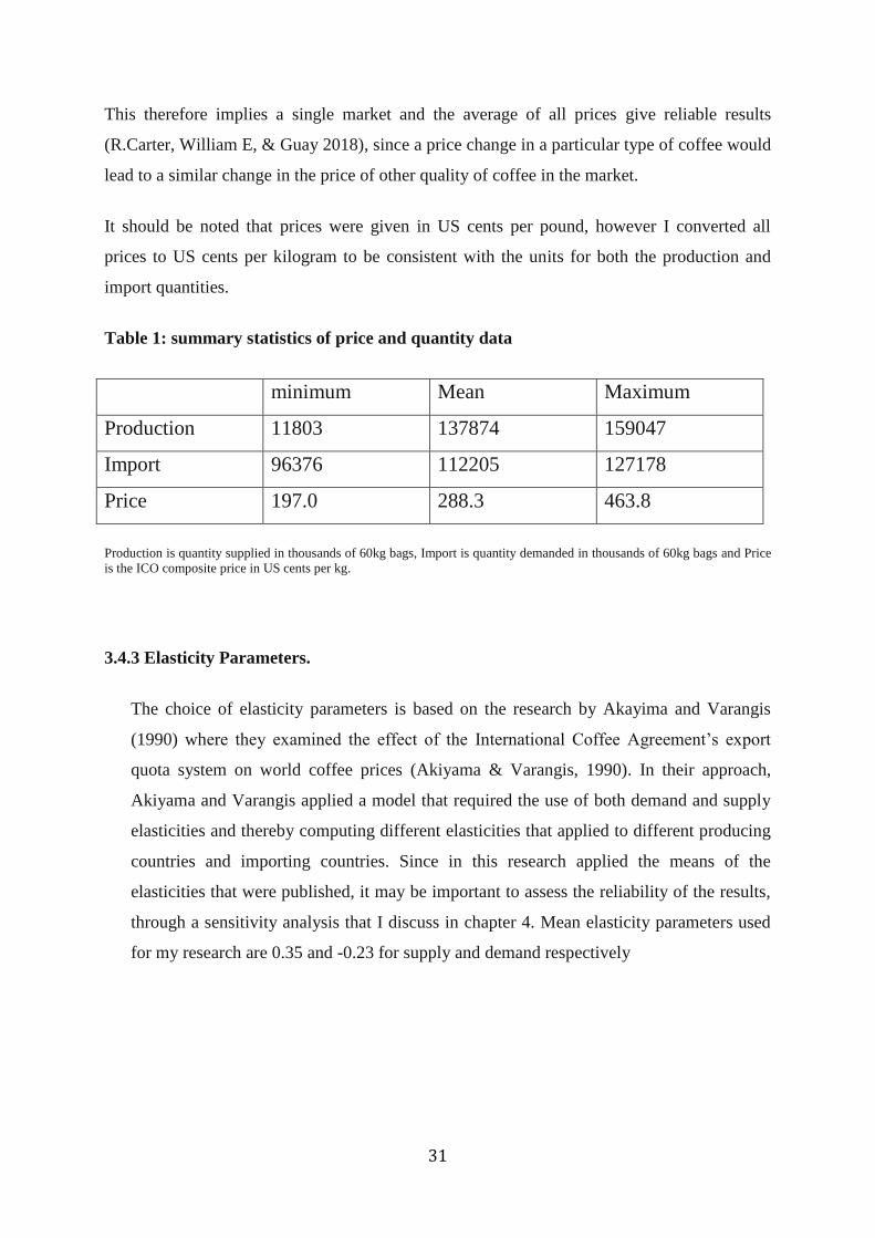
It should be noted that prices were given in US cents per pound, however I converted all

prices to US cents per kilogram to be consistent with the units for both the production and

import quantities.

Table 1: summary statistics of price and quantity data

minimum Mean Maximum

Production 11803 137874 159047

Import 96376 112205 127178

Price 197.0 288.3 463.8

Production is quantity supplied in thousands of 60kg bags, Import is quantity demanded in thousands of 60kg bags and Price

is the ICO composite price in US cents per kg.

3.4.3 Elasticity Parameters.

The choice of elasticity parameters is based on the research by Akayima and Varangis

(1990) where they examined the effect of the International Coffee Agreement’s export

quota system on world coffee prices (Akiyama & Varangis, 1990). In their approach,

Akiyama and Varangis applied a model that required the use of both demand and supply

elasticities and thereby computing different elasticities that applied to different producing

countries and importing countries. Since in this research applied the means of the

elasticities that were published, it may be important to assess the reliability of the results,

through a sensitivity analysis that I discuss in chapter 4. Mean elasticity parameters used

for my research are 0.35 and -0.23 for supply and demand respectively

32

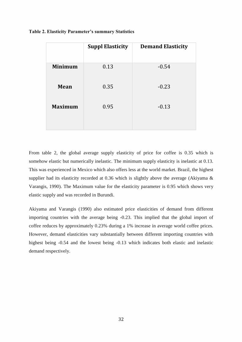
Table 2. Elasticity Parameter’s summary Statistics

Suppl Elasticity

Demand Elasticity

Minimum

Mean

Maximum

0.13

0.35

0.95

-0.54

-0.23

-0.13

From table 2, the global average supply elasticity of price for coffee is 0.35 which is

somehow elastic but numerically inelastic. The minimum supply elasticity is inelastic at 0.13.

This was experienced in Mexico which also offers less at the world market. Brazil, the highest

supplier had its elasticity recorded at 0.36 which is slightly above the average (Akiyama &

Varangis, 1990). The Maximum value for the elasticity parameter is 0.95 which shows very

elastic supply and was recorded in Burundi.

Akiyama and Varangis (1990) also estimated price elasticities of demand from different

importing countries with the average being -0.23. This implied that the global import of

coffee reduces by approximately 0.23% during a 1% increase in average world coffee prices.

However, demand elasticities vary substantially between different importing countries with

highest being -0.54 and the lowest being -0.13 which indicates both elastic and inelastic

demand respectively.

33

Chapter 4: Results and Discussions.

4.1 Introduction:

This section includes presentation of the results obtained after the analysis of the data using

the index approach as discussed in the methodology section in chapter 3. It also gives a

simple overview regarding the estimation procedure. All the analysis is done using Microsoft

Excel and R-studio. A shift in demand and supply are all given as percentages which

represents a percentage change in quantity demanded or supplied when price is held constant.

The results of demand and supply shifts exhibits both positive and negative values that

represent growth and reduction respectively. The positive shift indicates that a consumer is

willing to buy a higher quantity of coffee beans than in the previous period when price is

unchanged. For example, a 5% shift in demand implies that importing countries will bring in

5% more coffee than in the previous period even when price remain unchanged. Also, a 5%

positive shift in supply implies that exporters can produce 5% more coffee than in the

previous period at a constant price.

In addition to price and quantities, the choice of elasticity parameters used is the mean of all

obtained predetermined elasticities of demand and supply for demand and supply shift

respectively. This is a good representative of all countries where elasticity values were

obtained. Therefore, 0.35 and -0,23 are the respective elasticities of demand and supply used.

Both elasticity values are almost inelastic. A sensitivity analysis is performed later in this

section by using different values of the elasticity parameters to establish the consistency and

reliability of the results.

4.2 Results

Relative changes in quantity supplied and demanded together with relative changes in price

where estimated first in accordance the procedure of the index approach before application of

the elasticity parameters. These relative changes are represented in the table3 below:

34

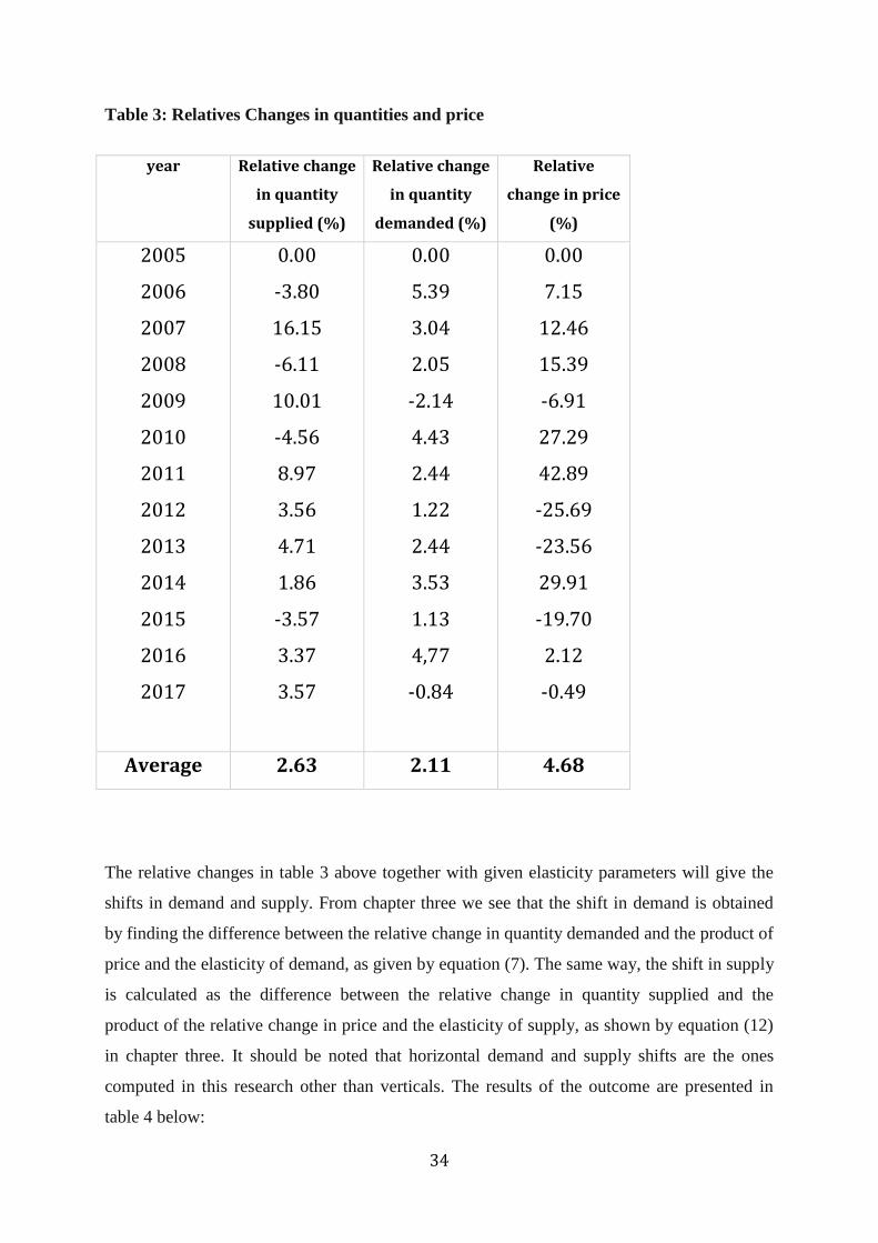
Table 3: Relatives Changes in quantities and price

year Relative change

in quantity

supplied (%)

Relative change

in quantity

demanded (%)

Relative

change in price

(%)

2005

2006

2007

2008

2009

2010

2011

2012

2013

2014

2015

2016

2017

0.00

-3.80

16.15

-6.11

10.01

-4.56

8.97

3.56

4.71

1.86

-3.57

3.37

3.57

0.00

5.39

3.04

2.05

-2.14

4.43

2.44

1.22

2.44

3.53

1.13

4,77

-0.84

0.00

7.15

12.46

15.39

-6.91

27.29

42.89

-25.69

-23.56

29.91

-19.70

2.12

-0.49

Average 2.63 2.11 4.68

The relative changes in table 3 above together with given elasticity parameters will give the

shifts in demand and supply. From chapter three we see that the shift in demand is obtained

by finding the difference between the relative change in quantity demanded and the product of

price and the elasticity of demand, as given by equation (7). The same way, the shift in supply

is calculated as the difference between the relative change in quantity supplied and the

product of the relative change in price and the elasticity of supply, as shown by equation (12)

in chapter three. It should be noted that horizontal demand and supply shifts are the ones

computed in this research other than verticals. The results of the outcome are presented in

table 4 below:

35

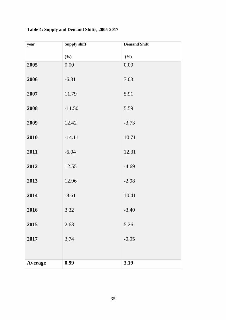
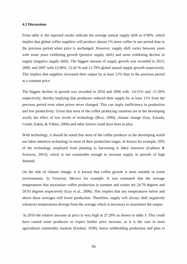
Table 4: Supply and Demand Shifts, 2005-2017

year

Supply shift

(%)

Demand Shift

(%)

2005

2006

2007

2008

2009

2010

2011

2012

2013

2014

2016

2015

2017

0.00

-6.31

11.79

-11.50

12.42

-14.11

-6.04

12.55

12.96

-8.61

3.32

2.63

3,74

0.00

7.03

5.91

5.59

-3.73

10.71

12.31

-4.69

-2.98

10.41

-3.40

5.26

-0.95

Average 0.99 3.19

36

4.3 Discussions

From table 4, the reported results indicate the average annual supply shift as 0.99%, which

implies that global coffee suppliers will produce almost 1% more coffee in one period than in

the previous period when price is unchanged. However, supply shift varies between years

with some years exhibiting growth (positive supply shift) and some exhibiting decline in

supply (negative supply shift). The biggest amount of supply growth was recorded in 2013,

2009, and 2007 with 12.96%, 12.42 % and 11.79% global annual supply growth respectively.

This implies that suppliers increased their output by at least 11% than in the previous period

at a constant price.

The biggest decline in growth was recorded in 2010 and 2008 with -14.31% and -11.50%

respectively, thereby implying that producers reduced their supply by at least 11% from the

previous period even when prices never changed. This can imply inefficiency in production

and low productivity. Given that most of the coffee producing countries are in the developing

world, the effect of low levels of technology (Rice, 1999), climate change (Gay, Estrada,

Conde, Eakin, & Villers, 2006) and other factors could have been in play.

With technology, it should be noted that most of the coffee producer in the developing world

use labor intensive technology in most of their production stages. In Kenya for example, 50%

of the technology employed from planting to harvesting is labor intensive (Gathura &

Sciences, 2013), which is not sustainable enough to increase supply in periods of high

demand.

On the side of climate change, it is known that coffee growth is most suitable in warm

environments. In Veracruz, Mexico for example. It was estimated that the average

temperatures that maximizes coffee production in summer and winter are 24.79 degrees and

20.03 degrees respectively (Gay et al., 2006). This implies that any temperatures below and

above these averages will lower production. Therefore, supply will always shift negatively

whenever temperatures diverge from the average which is necessary to maximiser the output.

In 2010 the relative increase in price is very high at 27.29% as shown in table 3. This could

have caused some producers to expect further price increase, as it is the case in most

agricultural commodity markets (Ezekiel, 1938), hence withholding production and plan to

37

supply more at a later date during further price increase, hence a fall in supply in 2011 by -

6.04%.

The small average annual supply shift (0.99%) for period of 2005-2017 implies that the

difference in positive growths and negative growths is very minimal. In the Equilibrium

Displacement Model, increase in supply and a decrease in supply have different impacts on

future prices. Therefore, frequent shifts in opposite directions (growth and negative growth)

explains the unexplained price frequent fluctuations in coffee market. A growth in supply

leads to excess supply that is sold at lower prices while a decline in supply create scarcity,

which eventually pushes prices even higher.

Demand shift from period 2005 to 20017 also vary substantially. A series of growth and

decline is also observed, and the average annual shift is 3.19%. This implies that on average

importers are willing to take 3.19% more coffee in a given period than the previous period

even when prices are held constant. 10.71% is the maximum annual growth which is the one

that corresponds to 2010 and -4.69% of 2012 is the highest decline in global demand for

coffee. On average the global demand for coffee is increasing each year. A bigger positive

average annual growth implies that demand growth is relatively higher than a decline in

demand. This can be explained by the level of necessity of coffee to world consumers

(Chiciudean, Funar, & Chiciudean, 2013), the world population structure (Gutierrez,

Villacorta, Cure, & Ellis, 1998), introduction of new market (Kim & Mauborgne, 1999) and

other factors that affect demand for coffee other than product own price. Most of these factors

were discussed in detail in chapter two.

However, since none of the periods exhibit zero shift, prices are also directly affected by the

continuous shifts in demand through the Equilibrium displacement model. At a constant price

and a given elasticity of demand, a positive shift in demand will result into competition on a

given product, pushing prices higher and a fall in demand will force suppliers to sell at a

lower price, hence lowering the price. Continuous shifts will push prices up and down thereby

creating price instabilities in the coffee market. The results of table 3 indicates that supply of

coffee shifts more than demand. Therefore, fluctuations in prices are influenced more from

the supply side rather than demand side.

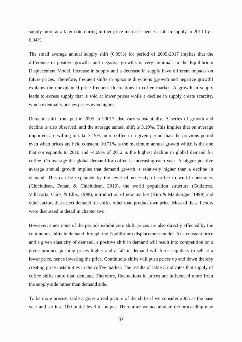
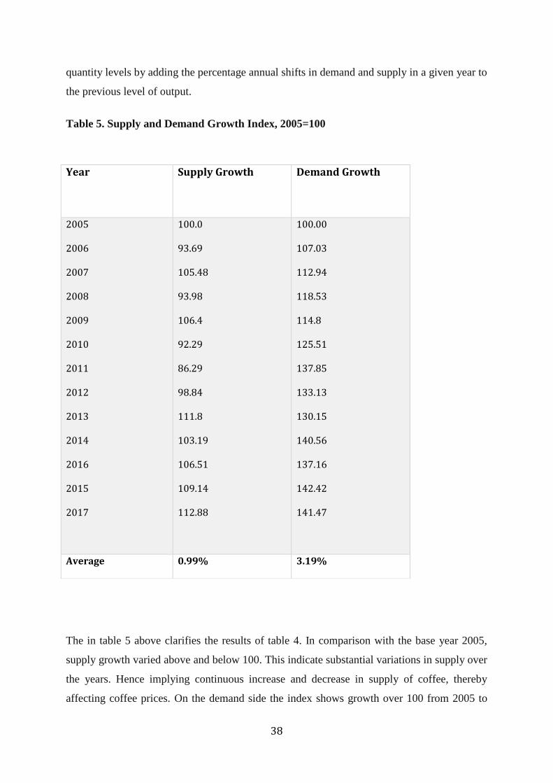
To be more precise, table 5 gives a real picture of the shifts if we consider 2005 as the base

year and set it at 100 initial level of output. There after we accumulate the proceeding new

38

quantity levels by adding the percentage annual shifts in demand and supply in a given year to

the previous level of output.

Table 5. Supply and Demand Growth Index, 2005=100

The in table 5 above clarifies the results of table 4. In comparison with the base year 2005,

supply growth varied above and below 100. This indicate substantial variations in supply over

the years. Hence implying continuous increase and decrease in supply of coffee, thereby

affecting coffee prices. On the demand side the index shows growth over 100 from 2005 to

Year

Supply Growth Demand Growth

2005

2006

2007

2008

2009

2010

2011

2012

2013

2014

2016

2015

2017

100.0

93.69

105.48

93.98

106.4

92.29

86.29

98.84

111.8

103.19

106.51

109.14

112.88

100.00

107.03

112.94

118.53

114.8

125.51

137.85

133.13

130.15

140.56

137.16

142.42

141.47

Average 0.99% 3.19%

39

2017. However, some declines in annual average growth were experienced in some years

although their effects are not big enough to reduce the index below 100. This shows that

demand is steadily increasing with only a few years of small decline.

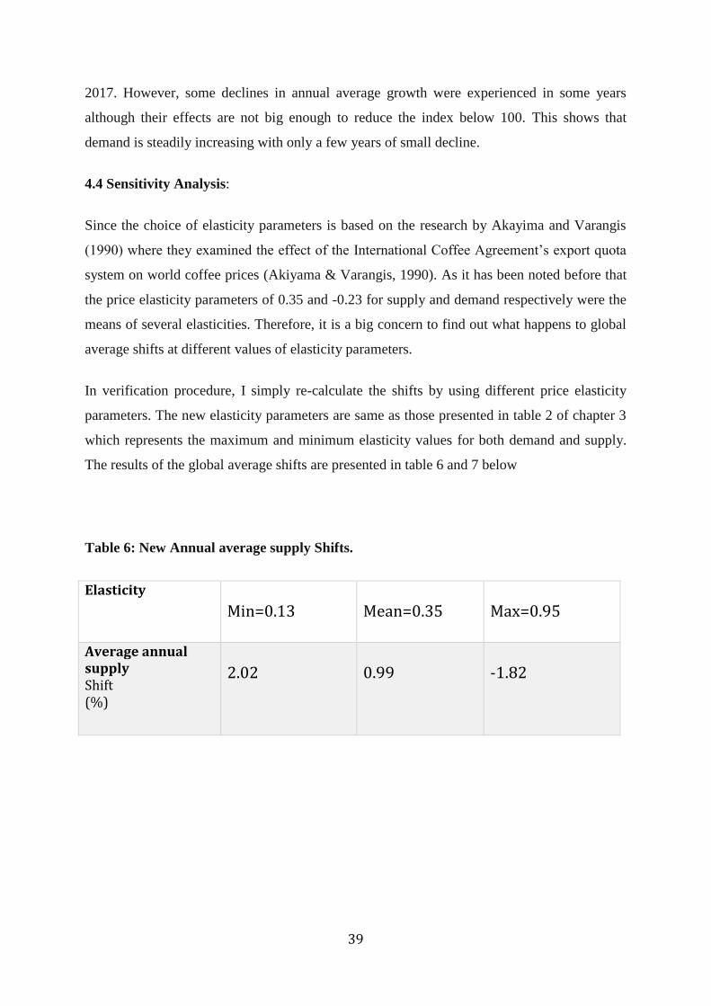
4.4 Sensitivity Analysis:

Since the choice of elasticity parameters is based on the research by Akayima and Varangis

(1990) where they examined the effect of the International Coffee Agreement’s export quota

system on world coffee prices (Akiyama & Varangis, 1990). As it has been noted before that

the price elasticity parameters of 0.35 and -0.23 for supply and demand respectively were the

means of several elasticities. Therefore, it is a big concern to find out what happens to global

average shifts at different values of elasticity parameters.

In verification procedure, I simply re-calculate the shifts by using different price elasticity

parameters. The new elasticity parameters are same as those presented in table 2 of chapter 3

which represents the maximum and minimum elasticity values for both demand and supply.

The results of the global average shifts are presented in table 6 and 7 below

Table 6: New Annual average supply Shifts.

Elasticity Min=0.13

Mean=0.35

Max=0.95

Average annual supply Shift (%)

2.02

0.99

-1.82

40

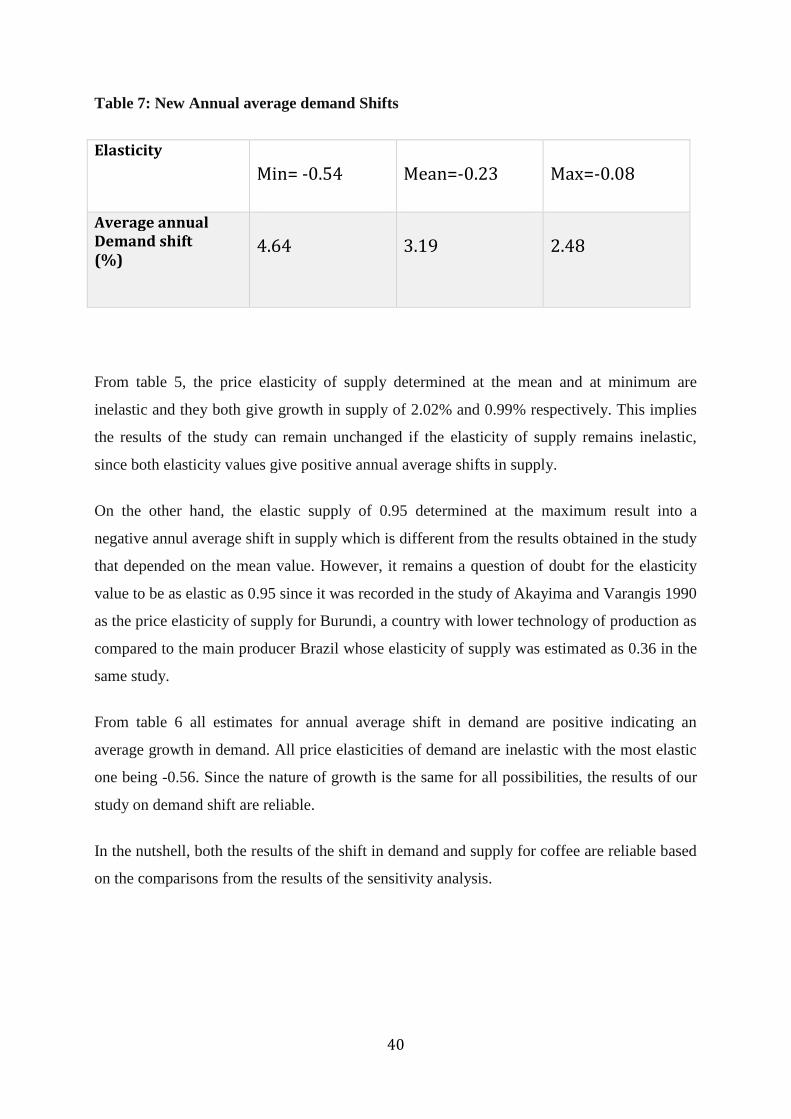
Table 7: New Annual average demand Shifts

Elasticity Min= -0.54

Mean=-0.23

Max=-0.08

Average annual Demand shift (%)

4.64

3.19

2.48

From table 5, the price elasticity of supply determined at the mean and at minimum are

inelastic and they both give growth in supply of 2.02% and 0.99% respectively. This implies

the results of the study can remain unchanged if the elasticity of supply remains inelastic,

since both elasticity values give positive annual average shifts in supply.

On the other hand, the elastic supply of 0.95 determined at the maximum result into a

negative annul average shift in supply which is different from the results obtained in the study

that depended on the mean value. However, it remains a question of doubt for the elasticity

value to be as elastic as 0.95 since it was recorded in the study of Akayima and Varangis 1990

as the price elasticity of supply for Burundi, a country with lower technology of production as

compared to the main producer Brazil whose elasticity of supply was estimated as 0.36 in the

same study.

From table 6 all estimates for annual average shift in demand are positive indicating an

average growth in demand. All price elasticities of demand are inelastic with the most elastic

one being -0.56. Since the nature of growth is the same for all possibilities, the results of our

study on demand shift are reliable.

In the nutshell, both the results of the shift in demand and supply for coffee are reliable based

on the comparisons from the results of the sensitivity analysis.

41

Chapter 5: Summary and Conclusion

5.1 Summary

This thesis consists of five chapters. Chapter one introduces the concept of coffee, its

importance and the benefits the world’s population derives from the commodity. It also

introduces the problem statement where the concept of price fluctuation in coffee market is

explained and how it has been experienced in different forms of coffee. Chapter one ends with

the research questions which acts as the basis for this thesis.

Chapter two gives the literature review of the thesis. It starts by introducing the concept of

demand and supply shift, the previous research that is based on the same concept as the one

used in this thesis. It further gives the difference between demand/supply shift and change in

quantity demanded/supplied. It still gives literature on the foundations of the studies

concerning measurement of supply and demand. Chapter two is extended to give an over view

of the world supply and demand in connection to coffee. Here, importers and exporters are

mainly discussed to represent demand and supply respectively. More discussion on countries

which export various forms of coffee is given, and finally the role of the ICA to impact coffee

demand, supply and price has been discussed at the end of this chapter.

Chapter three is the methodology section of this thesis. It starts by introducing the concepts of

demand shift and how it is estimated by an index approach that was first introduced by Marsh

(2003). It later gives a mathematical derivation of the expression that measures demand shift.

Furthermore, the concept of supply shift is also introduced in this section and later its

expression derived. Lastly, chapter three gives an overview of the data used which includes

both price, quantities and the elasticity parameters.

Chapter four shows the analysis, presentation of the results, discussion of the results and

verification of the reliability of the results.

Finally, chapter five contain the summary of the thesis and the conclusion, that represent the

general understanding of the outcome and some possible recommendation for further research

that can stem from this thesis.

42

5.2 Conclusion.

Understanding the reason behind price volatility of agricultural commodities is a topic of

debate among researchers and agricultural economists. In coffee market, prices are not stable.

This thesis helps to explain the price uncertainties in the coffee market by looking at the shifts

in demand and supply of coffee beans. This is achieved by answering the research questions

such as: (1) what is the level and nature of demand and supply growth/ shift of coffee? and (2)

what is the impact of supply and demand shift on coffee price fluctuations in the market?

By using an index approach developed by Marsh (2003), I examined the global supply and

demand growth for coffee beans. The results indicate that Supply of coffee shifts substantially

over time. This give an average annual shift in supply of 0.99%, thereby implying that

producing countries on average increase their production by almost 1% in one period than in

the previous period at a constant price. Demand shift also vary considerably over time with an

average annual shift of 3.19%. Therefore, importers take 3% more coffee in one period than

the previous when price is unchanged.

Since neither supply nor demand for coffee is constant over the period, prices are directly

affected. Therefore, continuous coffee price fluctuations are partly explained by continuous

shifts in demand and supply.

However, the shifts in supply for coffee varies more than the shift in demand. This is

represented by a smaller average annual shift in supply relative to demand shift. Continuous

patterns of growth and declines are more experienced from the supply side than the demand

side over the period from 2005 to 2017. This implies that the changes in prices are essentially

more influenced by shifts in supply than shifts in demand.

This research can be extended by disentangling the effects on either supply or demand which

are responsible for respective shifts. Factors such as substitution effect, income effect and

others can be studied independently using a similar approach to verify how much they

influence demand shifts. Also, different exogenous factors can be studied independently with

the same approach to see how much each influence supply shift of coffee given data

availability. This thesis integrates the effect of all factors without establishing the effect of

each individual economic or structural factors.

43

Refrencess

Akiyama, T., & Varangis, P. N. J. T. W. B. E. R. (1990). The impact of the International

Coffee Agreement on producing countries. 4(2), 157-173.

Balassa, B. J. W. d. (1990). Incentive policies and export performance in Sub-Saharan Africa.

18(3), 383-391.

Bettendorf, L., & Verboven, F. J. E. R. o. A. E. (2000). Incomplete transmission of coffee

bean prices: evidence from the Netherlands. 27(1), 1-16.

Brækkan, E. H. (2014). Why do Prices Change? An Analysis of Supply and Demand Shifts

and Price Impacts in the Farmed Salmon Market.

Brækkan, E. H., Thyholdt, S. B., Asche, F., & Myrland, Ø. J. E. R. o. A. E. (2018). The

demands’ they are a-changin’.

Brækkan, E. H., & Thyholdt, S. B. J. M. R. E. (2014). The bumpy road of demand growth—

an application to Atlantic salmon. 29(4), 339-350.

Bunn, C., Läderach, P., Rivera, O. O., & Kirschke, D. J. C. C. (2015). A bitter cup: climate

change profile of global production of Arabica and Robusta coffee. 129(1-2), 89-101.

Charveriat, C. J. O. P., Practice: Agriculture, F., & Land. (2001). Bitter coffee: How the poor

are paying for the slump in coffee prices. 1(1), 31-44.

Chiciudean, D., Funar, S., & Chiciudean, G. J. B. U. H. (2013). Study Regarding the

Influence of Country of Origin (COO) over the Consumer Decision-Making Process

in Buying Food. 70(2), 407-408.

Daniel, W. (2019). Coffee Imports by Country. Retrieved from

http://www.worldstopexports.com/coffee-imports-by-country/

Daviron, B., & Ponte, S. (2005). The coffee paradox: Global markets, commodity trade and

the elusive promise of development: Zed books.

Deaton, A., & Laroque, G. J. T. R. o. E. S. (1992). On the behaviour of commodity prices.

59(1), 1-23.

Dena, H. (2018). What is Arabica Coffee? Arabica vs. Robusta: 11 Tasty Differences.

Retrieved from https://enjoyjava.com/arabica-coffee/

Durevall, D. J. F. P. (2007). Demand for coffee in Sweden: The role of prices, preferences

and market power. 32(5-6), 566-584.

Ezekiel, M. J. T. Q. J. o. E. (1938). The cobweb theorem. 52(2), 255-280.

Gathura, M. N. J. I. J. o. A. R. i. B., & Sciences, S. (2013). Factors affecting small-scale

coffee production in Githunguri District, Kenya. 3(9), 132.

44

Gay, C., Estrada, F., Conde, C., Eakin, H., & Villers, L. J. C. C. (2006). Potential impacts of

climate change on agriculture: a case of study of coffee production in Veracruz,

Mexico. 79(3-4), 259-288.

Ghoshray, A. J. B. o. E. R. (2010). The extent of the world coffee market. 62(1), 97-107.

Goddard, E., & Akiyama, T. J. A. E. (1989). United States demand for coffee imports. 3(2),

147-159.

Gutierrez, A. P., Villacorta, A., Cure, J. R., & Ellis, C. K. J. A. d. S. E. d. B. (1998).

Tritrophic analysis of the coffee (Coffea arabica)-coffee berry borer [Hypothenemus

hampei (Ferrari)]-parasitoid system. 27(3), 357-385.

Hughes, J. J. J. A. J. o. A. E. (1969). Note on the US Demand for Coffee. 51(4), 912-914.

ICO. (2007). International Coffee Agreement 2007. Retrieved from

http://www.ico.org/ica2007.asp

ICO. (2019). Coffee Market Report: Coffee prices diverge in February 2019. Retrieved from

http://www.ico.org/documents/cy2018-19/cmr-0219-e.pdf

Kim, W. C., & Mauborgne, R. J. H. b. r. (1999). Creating new market space. 77(1), 83-93.

Lewin, B., Giovannucci, D., & Varangis, P. (2004). Coffee markets: new paradigms in global

supply and demand.

Marsh, J. M. J. A. J. o. A. E. (2003). Impacts of declining US retail beef demand on farm-

level beef prices and production. 85(4), 902-913.

Marshall, A. (1961). Principles of economics: An introductory volume: Macmillan London.

Mehta, A., & Chavas, J.-P. J. J. o. D. E. (2008). Responding to the coffee crisis: What can we

learn from price dynamics? , 85(1-2), 282-311.

Mikesell, R. F. J. T. A. E. R. (1963). International commodity stabilization schemes and the

export problems of developing countries. 75-92.

Mussatto, S. I., Machado, E. M., Martins, S., Teixeira, J. A. J. F., & Technology, B. (2011).

Production, composition, and application of coffee and its industrial residues. 4(5),

661.

Muth, R. F. J. O. E. P. (1964). The derived demand curve for a productive factor and the

industry supply curve. 16(2), 221-234.

Osorio, N. J. I. C. O., London. Available online: http://www. ico.

org/documents/globalcrisise. pdf. (2002). The global coffee crisis: a threat to

sustainable development.

Pichop, G. N., & Kemegue, F. M. J. S. W. b. j. (2005). International coffee agreement:

Incomplete membership and instability of the cooperative game. 2006.

45

Ponte, S. J. W. d. (2002). Thelatte revolution'? Regulation, markets and consumption in the

global coffee chain. 30(7), 1099-1122.

R.Carter, H., William E, G., & Guay , C. L. (2018). Principles of Econometrics. (5th ed.).

Rice, R. A. J. G. R. (1999). A place unbecoming: the coffee farm of northern Latin America.

89(4), 554-579.

Slob, B., Osterhaus, A. J. B. U. S., & Challenges of Fair Trade, B. F. T. A. O. (2006). A fair

share for coffee producers.

Smith, A. (1863). An Inquiry into the nature and causes of the Wealth of Nations: With a life

of the author, an introductory discourse, notes, and supplemental dissertations By JR

M'Culloch: Ad. and Ch. Black.

Smith, R. F. (1985). A history of coffee. In Coffee (pp. 1-12): Springer.

Subervie, J. J. J. o. A. E. (2008). The variable response of agricultural supply to world price

instability in developing countries. 59(1), 72-92.

Sun, C., & Kinnucan, H. W. J. S. J. o. A. F. (2001). Economic impact of environmental

regulations on southern softwood stumpage markets: a reappraisal. 25(3), 108-115.

Tomek, W., & Robinson, K. (2003). Agricultural Product Prices. NY. In: Cornell Univerrsity

Press.

Trostle, R. (2010). Global agricultural supply and demand: factors contributing to the recent

increase in food commodity prices (rev: DIANE Publishing.

Van der Vossen, H. J. E. A. (2009). The cup quality of disease-resistant cultivars of Arabica

coffee (Coffea arabica). 45(3), 323-332.

Wohlgenant, M. K. J. T. o. h. o. t. e. o. f. c., & policy. (2011). Consumer demand and welfare

in equilibrium displacement models. 0-44.

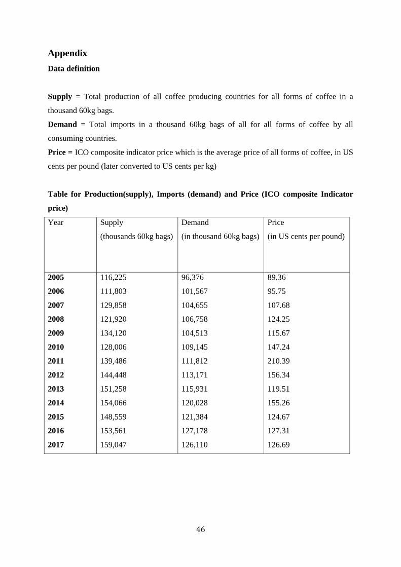
46

Appendix

Data definition

Supply = Total production of all coffee producing countries for all forms of coffee in a

thousand 60kg bags.

Demand = Total imports in a thousand 60kg bags of all for all forms of coffee by all

consuming countries.

Price = ICO composite indicator price which is the average price of all forms of coffee, in US

cents per pound (later converted to US cents per kg)

Table for Production(supply), Imports (demand) and Price (ICO composite Indicator

price)

Year

Supply

(thousands 60kg bags)

Demand

(in thousand 60kg bags)

Price

(in US cents per pound)

2005

2006

2007

2008

2009

2010

2011

2012

2013

2014

2015

2016

2017

116,225

111,803

129,858

121,920

134,120

128,006

139,486

144,448

151,258

154,066

148,559

153,561

159,047

96,376

101,567

104,655

106,758

104,513

109,145

111,812

113,171

115,931

120,028

121,384

127,178

126,110

89.36

95.75

107.68

124.25

115.67

147.24

210.39

156.34

119.51

155.26

124.67

127.31

126.69