Price Discovery, Volatility Spillovers and Adequacy of Speculation

in Cheese Spot and Futures Market

by

Marin Bozic and T. Randall Fortenbery

Suggested citation format: Bozic, M. and T. R. Fortenbery. 2012. “Price Discovery, Volatility Spillovers and Adequacy of Speculation in Cheese Spot and Futures Market.” Proceedings of the NCCC-134 Conference on Applied Commodity Price Analysis, Forecasting, and Market Risk Management. St. Louis, MO. [http://www.farmdoc.illinois.edu/nccc134].

Price Discovery, Volatility Spillovers and Adequacy of Speculation in Cheese Spot and Futures Market

Marin Bozic and

T. Randall Fortenbery*

Paper presented at the NCCC-134 Conference on Applied Commodity Price Analysis, Forecasting, and Market Risk Management

St. Louis, Missouri, April 16-17, 2012

Copyright 2012 by Marin Bozic and T. Randall Fortenbery. All rights reserved. Readers may make verbatim copies of this document for non-commercial purposes by any means, provided that this

copyright notice appears on all such copies.

* Marin Bozic (mbozic@umn.edu) is Assistant Professor in the Department of Applied Economics at the University of Minnesota-Twin Cities and T. Randall Fortenbery is Professor and Small Grains Endowed Chair in the School of Economic Sciences at the Washington State University. The funding support of the Economic Research Service of the U.S. Department of Agriculture under the Cooperative Agreement No. 144-PRJ29WK is gratefully acknowledged. Any opinions, findings, conclusions, or recommendations expressed in this publication are those of the authors and do not necessarily reflect the view of the U.S. Department of Agriculture. 

1

Price Discovery, Volatility Spillovers and Adequacy of Speculation in Cheese Spot and Futures Market

Practitioner’s Abstract: We investigate price discovery, volatility spillovers and impacts of speculation in the dairy sector. Examining the time series properties of cheese cash and implied futures price we find that the unit root hypothesis is strongly rejected for cash prices, while unit roots cannot be rejected for nearby futures prices in the framework that carefully controls for rollovers. To explain this result, we built a model that illustrates the time series properties of the nearby futures price series for a futures contract written on a second-order stationary cash series and identified the mean-reverting nonlinear dynamics that will occur at rollovers. Given the time series properties of the cash and futures series we propose an error-correction model using spreads between cash and the second nearby futures instead of the cointegration vector. To account for volatility dynamics we propose an extension of the BEKK variance model that we refer to as GARCH-MEX. That model does not restrict the sign of the additional regressors on the conditional variances, and can easily insure positive-definiteness of the conditional covariance matrix. We find that the flow of information in the mean model is predominantly from futures to cash, while volatility spillovers are bidirectional. It is possible that cash prices that include unfilled bid/offers react differently to increases in volatility in futures prices than sales cash prices, indicating that liquidity in the cash market is reduced with increase in conditional volatility of the futures price. Utilizing GARCH-MEX model we find strong evidence against the hypothesis that excessive speculation is increasing the conditional variance of futures prices. If anything, speculation may in fact be inadequate, and further research with daily speculative positions and high-frequency futures prices is needed to identify the effect of increased speculation on realized volatility of futures prices, bid-ask spread and magnitude of slippage.

JEL Codes: G13, Q13, C22 Keywords: implied cheese futures, unit root tests, volatility spillovers, speculation, GARCH-MEX

1. Introduction

There has been considerable interest in recent years concerning the overall performance of commodity futures markets, and the extent to which futures activity has led to price instability in cash markets. Much of the recent work in futures/cash price relationships has focused on the first moment of the price distribution and deep (large volume) markets (e.g. Irwin, Sanders and Merrin, 2009; Sanders, Irwin and Merrin, 2010; Hamilton, 2009; Gilbert, 2010). However, equally important are the relationships between the second and higher moments of futures/cash price distributions. Specifically, does price action in the futures market result in increased instability (volatility) in cash markets? As noted by Witherspoon (1993), market composition may impact market stability, and, as noted by Fortenbery and Zapata (2004), this may be more apparent in thin markets.

Dairy markets are unique for several reasons, not the least of which is the relative age of the futures markets for dairy. Dairy futures markets have existed since 1993, but underwent

2

continual re-design through the early 2000’s. The re-designs were in response to both changes in dairy market structure, and changes in dairy policy. Early work on dairy suggested that there were problems with the relationships between dairy futures and cash markets (Fortenbery and Zapata, 1997). In later work, it appeared that the issues had resolved themselves (Fortenbery, Cropp and Zapata, 1997; Thraen 1999). However, recent price action has again called into question the relationship between futures and cash markets for dairy, the impacts of technical innovation in the dairy sector on price performance, and the role of public policy in promoting price stability. Past work on price performance is dated given recent changes in both production and price policy.

This paper investigates price action and performance in dairy markets in several ways. First, the actual relationship between cash and futures price is studied. Both futures and cash markets have undergone significant changes over the last ten years, and their relationship to each other has not been examined recently. Futures changes include changes in futures contract design, delivery specifications, and the actual dairy commodities traded. On the cash side, the closing of the Green Bay Cheese Exchange, its replacement by a cash market in Chicago, and changes in both cash market structure and technology adoption in production may have impacted the cash/futures relationships.

We open the essay with a brief review of literature examining the information flow between cash and futures markets and the impact of speculators activity on both. In the second section, we describe the daily wholesale cash market for cheese as well as futures contracts for cheese and other dairy futures. A technique for calculating ‘implied’ cheese futures price for the period before actual cheese futures contract started trading is then discussed. Time series properties of cash and nearby futures cheese price are evaluated next. The fourth section discusses in further detail the concepts of causality as they are commonly used in the applied econometrics literature. An error-correction model with a GARCH-BEKK variance structure is then proposed as an appropriate analytical framework given the results of unit root tests, followed by the discussion of empirical results. To examine the influence of speculators on price volatility new GARCH model is proposed that nests BEKK variance structure while allowing flexibility in the direction of impact of additional regressors included in the variance model. We apply this model to evaluate the adequacy of speculation in the Class III milk futures. Paper concludes with policy implications and suggestions for further research.

1. Literature review

Do futures markets, by facilitating speculation, increase cash price volatility? Early work by Working (1960, Feb) in onion futures demonstrated that speculative support at harvest time reduced both seasonal price range and price adjustments at the end of the marketing year, as needed adjustments were better anticipated and incorporated in prices earlier. Gray (1963) extended Working’s analysis to include seasonal patterns in onion cash prices after the trade in onion futures was prohibited. He found that pronounced seasonality in cash prices, reduced during the years of intense futures trading, had returned after onion futures were discontinued.

In addition to reductions in seasonality and earlier anticipation of adjustments needed at the end of a marketing year, futures may reduce year-to-year price fluctuations. Whereas the first two

3

effects are mediated through the impacts of futures prices on storage decisions, the last effect will be present if the futures prices are perceived as reliable guides to production planning, and farmers engage in what Working (1962) calls anticipatory hedging.

Powers (1970) investigated live beef and pork belly markets around the time futures contracts were first introduced for these commodities. He modeled weekly cash prices as the sum of two components assumed to be uncorrelated: the systematic component associated with fundamental economic conditions and the error or random component which represents noise and disturbance in the price system. He employed a variate difference method to separate systematic and random components, and then calculated the variance of the random part separately for four year periods before and after the introduction of futures markets. For both commodities he analyzes, he found that the variance of the noise decreased after futures contracts were introduced, but offered no statistical evidence that reduction can be attributed to information services performed by the futures market. Taylor and Leuthold (1974) examined the impact of new futures market on the variance of average annual, monthly and weekly of livestock cash prices, and found that while weekly and monthly variances decreased, the effect on annual variability was not statistically significant. They conjecture that the differential effect of futures market introduction on different frequencies may be due to a contract design, as livestock contracts at that time did not trade for horizons sufficiently long to influence the behavior of livestock breeders, given the long reproductive cycle of cattle. Brorsen, Oellerman and Farris (1989) extended the analysis to daily live cattle cash price variability. In their theoretical model, faster information assimilation was enabled by the introduction of a futures market, and the transmission of that information to the cash market resulted in increased daily variability in cash prices, and a reduction in cash price autocorrelation. Empirical analysis encompassing periods before and after live cattle futures were introduced confirmed their hypotheses. They concluded that live cattle futures improved the cash market efficiency, but increased short-term price risk.

Cox (1976) proposed that introducing of a futures market may attract a new set of traders who acquire and process information in order to predict future cash prices, but do not handle the physical commodity. Speculators participating in the futures market may be more informed about the future supply and demand conditions than commercial parties. If that is the case, the addition of a futures market will enable the cash market to more quickly absorb the most recent information. The testable hypotheses emerging from Cox’s work are twofold. First, the addition of a futures market will change the time series properties of the cash prices, with autoregressive components in cash price process fading in importance. In addition, expected prices will be more reliable predictors of future cash prices, i.e. the variance of the price-forecast error will decrease.

Turnovsky (1983) adds to the literature by showing that in the case where producers are risk averse, introduction of a futures market will affect not only the information set based on which the expectation of future spot prices are made, but also the slopes of the supply and inventory demand functions as they depend on the degree of price stability. He found that under a wide

4

range of behavioral assumptions the futures market reduces both cash price volatility and long run average spot price.

Newbery (1987) extended Turnovsky’s basic idea that futures markets can insure against risk, and thus increase the supply of otherwise risky activities. He built a model in which farmers must choose among two competing plant breeds, one that produces less output but with no uncertainty and another that is risky, but produces higher average yield. Once hedging with futures becomes available farmers may trade some price risk for increased production risk. If a sufficient number of producers exhibited such behavior, then the volatility of cash price may in fact increase. In his study the futures market did not destabilize cash price through speculative activities but through the impact on producer decision-making.

The price discovery function of the futures market is the ability of the futures prices to quickly absorb new price-relevant information and transmit it through to the cash prices. Price discovery has been the subject of a vast empirical literature, and some examples include Garbade and Silber (1983), Oellerman and Farris (1985), Schroeder and Goodwin (1991), Fortenbery and Zapata (1993, 1997), Zapata and Fortenbery (1996), and Yang and Bessler (2001). In early work, dynamic models in either price levels or differenced prices were utilized. With development of time series methods that can appropriately address nonstationarity of prices, researchers have started using co-integration models to analyze price discovery. Of particular interest for the present study are articles analyzing the price discovery in thin markets. In such settings, Brockman and Tse (1995), Fortenbery and Zapata (1997), Mattos and Garcia (2006) and Ivanov and Cho (2011) find that price discovery can be hampered by the lack of liquidity or institutional constraints. This is manifested as either lack of cointegrating relationship between cash and futures market or lower information share of futures market in the price discovery process.

Impact of speculation on price levels and volatility dynamics has been recently investigated in several papers. For example, in his testimony before the U.S. Senate, Masters (2008) argued that institutional investors are among the major factors affecting commodities prices, and Gilbert (2010) argues that index futures investment was the principal channel through which monetary and financial activity have affected food prices in the second half of 2000s. However, Irwin, Sanders and Merrin (2009) argue that bubbles in futures prices are not likely, and find that speculative positions do not Granger cause futures price changes. Earlier work by Streeter and Tomek (1992) finds that volatility of soybeans futures decreases as Working’s T index of speculation increases. Du, Yu and Hayes (2011) find a positive impact of speculation on crude oil price volatility. Using more detailed data, Brunetti and Büyükşahin (2009) and Brunetti, Büyükşahin and Harris (2011) find that increased speculative activity does not destabilize financial markets, and in fact predicts lower realized volatility in crude oil and other markets they analyze. However, Tang and Xiong (2010) find that futures prices of different commodities in the US became increasingly correlated with each other and this trend was significantly more pronounced for commodities in the two popular GSCI and DJ-UBS commodity indices. Büyükşahin and Robe (2011) note that correlations between the returns on commodity and on

5

equity indices increase significantly amid greater activity by speculators in general and one type of traders in particular – hedge funds. These results may indicate that while speculators overall help increase market liquidity, they increase the sensitivity of commodity prices to macroeconomic shocks.

2. Data

In this paper, we are interested in evaluating information flows between spot and futures markets in the dairy sector. While we are ultimately interested in price discovery for milk price, there is in fact no national spot market for fluid milk. Given that the fluid milk prices are linked to the prices of milk used in cheese production, the second best approach to investigating cash-futures relations seems to be to look at the cash and futures markets for cheese. This section describes the aspects of the milk pricing environment in the U.S. that are relevant to my research question.

Pricing of milk in the U.S. is highly regulated under Federal Milk Marketing Orders (FMMO). Three main objectives of the FMMOs are: 1) insuring market price stability, 2) preventing processors from exercising market power over milk producers and 3) insuring adequate supply and orderly marketing of fluid milk.

The primary instrument FMMOs use to achieve these objectives is to set minimum prices that handlers of Grade A milk must pay to farmers. The fundamental principle currently used to determine minimum milk price is measure the value of milk as a function of milk ingredients that have desirable nutritional qualities: milk protein, butterfat, and milk solids (lactose, whey proteins, minerals, lactic acid).

Values of the principal milk components are inferred from derived dairy products like cheese, butter, dry whey and non-fat dry milk. Finally, in order to calculate a minimum price of milk, a standard composition of milk in terms of percentages of each ingredient is assumed. In particular, the standard used by the USDA assumes that milk used for the production of cheese consists of 3.5% butterfat, 2.99% protein and 5.69% other solids. The USDA differentiates between milk used for cheese production and milk used in production of dry products. The former is referred to as Class III milk, and the latter Class IV milk. Similarly, milk used for fluid consumption is termed Class I milk, and its minimum price exceeds the price of manufacturing milk. For milk produced for consumption, the ‘ingredient’ that carries the additional value is the location of marketing.

The flowchart in Figure 1 presents the procedure the USDA uses to arrive at the Class III and Class IV manufacturing milk prices. First, major producers of butter, dry whey, nonfat dry milk and cheese are surveyed weekly. Monthly averages of these prices, with weeks weighted by volume, are used to infer the average monthly price of the ingredients. In particular, let B

tP be the

average surveyed price of butter in month t . Then the value of butterfat is calculated as

B B Bt t tbf P C Y (1)

where BtC is the USDA’s estimate of the national average cost of manufacturing a pound of

butter, termed make allowance in industry jargon, and BY is the yield, i.e. the pounds of butter that can be manufactured from one pound of butterfat. This is assumed equal to 1.20. Make

6

allowances for dairy products change very infrequently, and only after a lengthy administrative process that involves public hearings where manufacturers present arguments on what should be deemed a fair assessment of production costs. Currently, the butter make allowance stands at $0.1715. This value changed only 4 times since the beginning of 2000. Similar to butterfat, the value of other milk solids is inferred from a surveyed value of dry whey:

W W Wt t ts P C Y (2)

where WtP is the price of dry whey and W

tC is the dry whey make allowance, currently set at

$0.1991 per pound. Although the name of the final product may indicate that it contains nothing but solids, it is the fact that dry whey does contains some moisture. USDA formula assumes that yield WY equals 1.03, i.e. a pound of other milk solids will make 1.03 pounds of dry whey.

Calculating the value if nonfat milk solids, tnfs , proceeds in exactly the same fashion. The

nonfat dry milk make allowance, currently at $0.1678/lbs, is deducted from the surveyed price for nonfat dry milk, and the difference is then multiplied by 0.99.

The dairy product that serves as the base for the calculation of the protein price is cheddar cheese that is 4 to 30 days old, sold in 40 pound blocks or 500 pound barrels. Cheese yield depends nonlinearly on the amount of protein and butterfat in milk, as the interaction of these components is recognized as an important contributor to yield. The following formula accounts for that effect

0.9 1.17C C CP C C CPBt t t t t tpr P C Y P C Y bf (3)

where CtP is the surveyed price of cheese, C

tC is the cheese make allowance, currently at

$0.2003/lbs, CPY is the cheese yield from protein, and CPBY is the multiplier accounting for interaction effects between protein and butterfat. The assumed ratio of protein to butterfat in cheese is 1.17 which explains the last multiplier.

After the prices of all ingredients have been calculated, arriving at the final Class III and Class IV prices is a simple two-step process. First, the price of skim milk is calculated for both classes. For Class III, the skim milk price is calculated as the weighted average of protein and other solids.

3 3.1 5.9t t tC skim pr os (4)

Similarly, the Class IV skim milk price is

4 9.0t tC skim nfs (5)

Finally, Class III and Class IV milk prices are obtained by adding a butterfat price to skim milk prices.

3 0.965 3 3.5

4 0.965 4 3.5t t t

t t t

C C skim bf

C C skim bf

(6)

7

Unlike prices for particular ingredients, the prices for skim milk and final class prices are expressed as U.S. dollars per hundredweight (100lbs). At each step of the process, derived prices are rounded to four decimal points.

The Chicago Mercantile Exchange (CME) operates a spot market for cheese that trades each business day from 10.45-10.55 a.m. Cheese trades in carloads weighing between 40,000 and 44,000 pounds, packed as either 40lbs blocks or 500lbs barrels. Cheese may not be less than four days or more than 30 days of age on the date of sale. This market is often regarded as thin, given that only a handful of trades occur each day, and on 40% of the trading days no sale occurs at all. Nevertheless, it is precisely this market that serves as a the price discovery center for many cash dairy products, and the weekly NASS national survey price for cheese exhibits a 0.99 correlation with the previous week average spot cheese price.

Perhaps due to the thinness of the CME cash cheese market, it is a custom to report the last bid or last offer as the daily closing price if they remained uncovered or unfilled. This renders public data on spot cheese prices problematic for econometric analysis, as the prices are often not transaction prices and are not indicative of the current market equilibrium price.

To address this issue,we have obtained the intraday cash market data that specifies each price quote as either sales, bid or offer, and have used only the last sales price of the day in my analysis. If no trade has occurred on a particular day, we use the last observed transaction price from an earlier date.

Next, we need to obtain a cheese futures price. Although cheese futures were among the first dairy futures contracts created in the early 1990s, the contracts were discontinued after the federal milk marketing order reform of 2000. Since 2000 on there were no cheese futures available, until new cash-settled cheese futures contract started trading in July 2010. As presented in the second essay of this thesis, the correlation between announced Class III price and the monthly average NASS survey cheese price is 0.95, which means we could use Class III futures, appropriately scaled, as a proxy for cheese futures prices. However, if we seek to pin down current market expectation of the price of cheese in the future, then such an approach is still imperfect and subject to substantial measurement error, as it disregards the changes in expectations regarding prices of other milk components that enter the Class III milk price formula: namely, butterfat and other milk solids.

From 2000 until September 2005, the only dairy futures contracts publicly available where Class III and Class IV milk and a deliverable butter contract. We can use the butter contract to infer the implied futures price of butterfat. To calculate the implied futures price of cheese, we would need to know the implied futures price of protein, in addition to butterfat. Using Class III and Class IV futures and the implied price for butterfat, we calculate the implied futures price for Class III and Class IV skim milk. In order to obtain an implied protein price, we need implied futures price for other milk solids. Class III and IV skim milk prices are functions of butterfat and other milk solids, and butterfat and nonfat milk solids respectively. Using only the implied skim milk prices we cannot uniquely identify the implied futures price of the three ingredients that enter the formulas for skim milk prices. However, if we make an assumption about the future price ratio of nonfat milk solids to other milk solids then we can use implied Class III and Class IV skim milk price to estimate the conditional expectation of implied futures price for other milk solids as well as protein.

8

In particular, we assume that the ratio of the monthly announced average price for nonfat dry milk and dry whey is an AR(1) process. When calculating conditional expectations of the implied cheese futures at time t , we only use the observations of dry whey and nonfat dry milk prices available on that date in fitting the coefficients of the stated AR(1) regression. In this way the conditional expectation of the implied futures cheese price is obtained using only information available to traders.

Measurement errors using this approximation method arises from two sources. First is uncertainty regarding the ratio of nonfat dry milk to dry whey prices. The other potential source of error comes from the fact that the butter contract is not cash-settled against the NASS survey price. Instead, physical delivery is required at certified warehouses. This may be cause for additional differences at settlement between the CME cash cheese price and the implied cheese futures price calculated using the butter futures contract.

In September 2005 cash-settled butter contract was introduced. From that point on we use the cash-settled butter contract in calculating the implied cheese futures price. In May 2007, a dry whey contract was introduced. This allows us to identify the implied futures price of other milk solids, and consequently the last source of measurement error is removed. Figure 3 compares the implied cheese futures obtained using all three approximation methods and, for the period after July 2010, actually observed cheese futures prices. While there is some difference between the implied cheese futures price in the early months of 2007 as obtained using various approximation methods, all methods give very similar results for the predominant part of the past four years. In particular, we find that the absolute difference between implied and observed cheese futures is never higher than 2 cents per cwt., which probably reflects the transaction costs of riskless arbitrage (i.e. bid-ask spread, assuming that exchange members can trade without paying any transaction fees) combined with the effects of rounding to four decimal points at each step in deriving the various class milk prices.

This results in a total sample period that spans July 11, 2000 (the first day Class IV contract traded) through April 4, 2011, the last day for which cash price data was available to us. The total number of observations is 2670.

2. Time Series Properties of Cheese Cash and Futures Prices.

In order to appropriately model the information flow between cash and futures markets, it is important to understand the time series properties of both cash and futures price series. In particular, when prices are non-stationary, estimating models in price levels may result in spurious regressions. On the other hand, if prices are co-integrated, estimating models with differenced series will result in a misspecified model, and the cointegration framework should be utilized instead.

In this section we evaluate the time series properties of cheese cash and futures prices. We find that the null hypothesis of unit roots presence is strongly rejected for cash prices. Results are mixed for nearby futures prices, and vary with data frequency, horizon to maturity and the method of constructing lagged prices in regressions used for estimating Augmented Dickey-Fuller tests. Further, the simple difference between concurrent cash and nearby futures price is

9

strongly mean-reverting. In what follows we review the theoretical predictions for time series properties of cash and futures prices and build a simple model to illustrate the kind of nonlinearities that a nearby futures price series may exhibit when a cash price series is second-order stationary. The patterns observed in unit-root results closely match predictions of the illustrative model.

2.1. Unit root tests

I employ three types of unit root tests: the Dickey-Fuller (DF), Augmented Dickey-Fuller (ADF) with automatic lag selection based on AIC criteria and the Phillips-Perron test (PP). For the Dickey-Fuller (1979) test for unit roots in the absence of serial correlation we estimate a regression with an included constant term but no time trend. The null hypothesis assumes that true process is a random walk.

The estimated regression is:

1t t ty y u (7)

with the assumed true process under the null hypothesis of

21 , ~ 0,t t t ty y u u N (8)

Under the null hypothesis, ˆˆ ˆ1 / has a non-standard distribution, and for large samples

critical values for rejecting the null at 10%, 5% and 1% confidence level are -2.57, -2.86 and -3.43 respectively.

Augmented Dickey-Fuller tests (Said and Dickey, 1984) correct for serial correlation in residuals by including higher-order autoregressive terms in the regression. Similar to equation (7) above, we estimate an autoregression that includes a constant term. The null hypothesis is that the data are generated by a unit root autoregression with no drift.

The estimated regression is

1 1 2 2 1 1 1...t t t p t p t ty y y y y (9)

where 1t t ty y y . The true process is assumed to be the same specification as in (9) with

0 and 0 . The OLS t test for 0 has a non-standard distribution and critical values are the same as in Dickey-Fuller test listed above. To select the appropriate lag structure, we estimate the model with 0 through 20 lags, and choose the specification with the lowest AIC criteria.

Finally, we also estimate the Phillips-Perron (1988) tests for unit roots in presence of serial correlation. The estimated regression is

1t t ty y u (10)

with the true process assumed to be:

10

1t t ty y u (11)

The test statistic used in this test is

1/2 ˆ2 20, 0,

ˆ

ˆˆ 1 1ˆ ˆˆ ˆ/ˆ 2

T

T

Tt T T T T

T

TZ

s

(12)

where 1,

1

ˆ ˆ ˆT

j T t t jt j

T u u

, ˆtu are OLS sample residuals from the estimated regression,

1 2

1

ˆT

T tt

s T k u

, k is the number of parameters in estimated regression, ˆˆT

is the OLS

standard error for ̂ , and 20, ,

1

ˆ ˆ ˆ2 11

q

T T j Tj

j

q

is the Newey-West estimator of error

variance with q lags chosen based on minimial AIC criteria in the ADF lag selection process.

Critical values for tZ are the same as in Dickey-Fuller and Augmented Dickey-Fuller tests.

RATS 8.01 was used for these tests as it provides the user with easy-to-use commands for the tests as well as selecting the optimal lag structure to be used in the ADF and Phillips-Perron tests.

It has been noted that results of unit-root test may vary with data frequency (Tomek and Wang, 2007), so we estimate these tests for both daily and weekly data frequency. In addition, since CME cash market for cheese is not very liquid, and sales transactions do not occur on about 40 percent of trading days in the sample, we construct an irregular frequency data keeping only those days when the cash market did in fact record a sales transaction either in 40lbs cheese blocks or 500lbs cheese barrels.

Perhaps due to low cash market liquidity, it is a custom in the cheese industry to report the last uncovered offer or last unfilled bid as the closing cash price for the day. While our primary cash price series only contains sales records, it may be of interest to examine if any of the results regarding cash/futures information flow are sensitive to the choice of cash price series (i.e. closing sales price vs. closing prices that may be a bid or offer). For that reason, we perform unit root tests on these publicly reported closing cash prices as well, and denote them with a (B/O) suffix to differentiate from the regular sales price series. In addition, we account for potential seasonality in cash prices by testing for the presence of unit roots in the residuals from regressions of cash prices on quarterly indicator variables rather than testing for unit roots in cash prices directly.

I examine the sensitivity of ADF test results to the specification of lagged prices in the estimated regression. Recall that the futures price series is always an n-th nearby series, i.e. concatenation of segments taken from different futures contract months at the time when those contracts were the n-th contract to maturity. Denote by i

tf a futures price on time t for a contract expiring at iT .

Then jth-nearby is a sequence of futures prices that can be represented as

11

1 1 1 1 1 1 1

1 1 1 21 1 2 1... , ,..., , , ,..., , ...

i j i j i j i j i j

i i i i i i ij t t T T T T TF f f f f f f f

(13)

For example, the 2nd nearby futures price series is constructed by taking the prices of the February contract in the month of January, the March contract in the month of February, etc. Notice that in such a nearby series from time to time two consecutive prices will correspond to different contract months. For example, when the January contract settles, the 2nd nearby futures price will be the one from March, while one day earlier, i.e. on the last day the January contract traded, the 2nd nearby futures price will refer to a February contract futures price. As a consequence, using inbuilt software commands that do not account for this information will produce differenced prices for equation (9) that are occasionally corresponding to different contract months. To check if this is influencing the test results, we estimate a regression that insures that differenced prices always come from the same contract month, but is other otherwise equivalent to regression estimated by the inbuilt RATS command, i.e. the number of lags are determined via AIC criteria. In particular, we estimate the following regression

1 1 2 2 1 1 1...t t t p t p t tf f f f f (14)

where 1i i

t t tf f f and right hand side variable 1 1i

t tf f .

Finally, to account for possible sensitivity to the choice of rollover date, we perform unit root tests of nearby series that are constructed by rolling over included contracts on the days when the 1st nearby contract expires, as well as on the day when the 1st nearby has 3 trading days to maturity left.

Results of the unit root tests are presented in Table 1. The null hypothesis of unit roots is strongly rejected for cash cheese prices. This holds true irrespective of the data frequency used, whether 40lbs blocks or barrels are examined, and whether the series is based on sales prices or publicly reported daily closing prices that may include unfilled bids and uncovered offers.

The situation is more complex in unit root test results for nearby futures prices. The ADF test for unit roots rejects the null for the second nearby futures series at a 5% confidence level irrespective of the data frequency used, while data frequency seems to matter for the 3rd, 4th and 5th nearby series. Irrespective of the rollover procedure used, tests done with weekly data are more likely to reject a unit root. The Phillips-Perron statistics are generally higher for weekly data frequency than those obtained using daily and sales only frequency. For daily and sales-only data, with the exception of the 1st nearby contract, the ADF test statistic falls as time-to-maturity increases, i.e. the ADF t-statistic is higher for the 2nd nearby than for the 3rd nearby, etc. The most striking result is the difference in t-statistics from the regular ADF regression that does not account for contract rollovers in constructing differenced prices, and the equivalent regressions that do. When regressions like (14) are estimated, the t-statistics next to lagged price of the same contract are very small, and the null hypothesis of unit roots is never rejected. This happens regardless of data frequency, time to maturity horizon and rollover method used. Regressions (14) evaluate the time series properties of within-contract segments, ignoring dynamics at contract rollovers. Therefore, these results suggest that unit root results based on ADF regressions may be driven by the nature of the price changes at the rollover time. In particular, this indicates that nearby futures price series are nonlinear - martingales within each contract segment, and mean-reverting at contract rollovers. As rollovers occur more frequently for weekly

12

data the explanation offered above is consistent with unit roots tests more strongly rejecting the null for weekly data series.

Of special interest is evaluating the time series properties of the cash-futures price spread, denoted ,n td and defined as the difference between contemporaneous average cash prices and n-th

nearby futures price , ,n t t n td c f . In this context the cash price is a simple average of blocks

and barrels cash sales prices for a particular day. Results are reported for spreads calculated using second and fifth nearby futures, and spreads are always found to be strongly stationary. If the fifth nearby futures were indeed nonstationary, and if the cash price was truly stationary, then no linear combination of the two series could be stationary. The fact that the null is strongly rejected for spreads using the fifth nearby futures is additional evidence suggesting there are nonlinearities in the nearby futures prices.

There are three questions that naturally arise as a reaction to these results. First, what does economic theory suggests about the time series properties of cash and futures commodity prices? Second, what kind of nonlinearities should we expect in nearby futures prices, when cash prices are stationary? And finally, what is the appropriate way to model information flows between cash and futures markets in the face of observed stationarity in cash prices and nonlinearities in nearby futures prices. The first two questions are answered in the next subsection, while the model specification issues are left for the next part of the paper.

2.2. Economic theory and time series properties of agricultural cash and futures prices

Early studies of cash/futures linkages used regression in price levels or differenced series (e.g. Oellerman and Farris, 1985). However, in many commodities, and especially when using daily data, researchers have found that both cash and futures contain unit root (e.g. Schneider and Goodwin, 1991; Ivanov and Cho, 2011). These findings have been disputed both on theoretical and statistical grounds. As far as theory is concerned, it has been claimed that agricultural price theory does not support the hypothesis that all shocks to prices are persistent (Tomek and Wang, 2007). Furthermore, misspecified models that do not account for structural breaks may bias the results towards accepting the null hypothesis of unit root presence, and unit roots test that have low power will not be effective in differentiating between integrated and stationary, but highly persistent time series (Geweke and Porter-Hudok, 1983).

Theoretical priors regarding time series properties of cash and futures prices are remarkably different. As far as cash price is concerned, the fundamental property of prices emerging in perfectly competitive markets is the necessity of zero long-run economic profit for the marginal producer. That condition implies that profit margind will be a mean-reverting time series. Consequently, if the long-run industry average cost curve is flat (a case of constant returns to scale), any permanent shift in the demand function will produce only temporary shock to cash prices, while permanent changes in input costs will shift the long-run average cost curve and thus induce a structural change in cash price series. Even with constant long run average costs, if production cannot adjust quickly to demand shocks in the short run, cash prices may exhibit high a degree of persistency and rather slow reversion to long-run averages. Finally, if returns to scale

13

are either decreasing or increasing, shifts in demand will manifest as permanent shocks to cash price series.

While the time series properties of cash prices are argued based on production theory, the time series characteristics of futures price series emerge from finance theory. If the futures market is efficient (i.e. if futures prices fully account for all available information) then prices within a single contract will be martingales if the marginal risk premium is zero, submartingales if marginal risk premium is positive (i.e. futures are downward biased and traders having long position are rewarded), and supermartingales if the marginal risk premium is negative (i.e. futures are upward biased and traders having short position are rewarded). In each case, by deducting the marginal risk premium we can arrive at a martingale series whose direction of change cannot be predicted based on concurrently available information. From this it follows that whether the risk premium is present or not, efficient futures prices will be nonstationary, i.e. all shocks to futures prices are permanent.

Suppose now that there exists a second-order stationary cash price series for some commodity, and that a futures contract is written on that commodity. Assume further that there is no basis at futures contract expiry, i.e. the terminal futures price equals the cash price prevailing at contract expiry. Finally, assume that futures prices are efficient and embody no risk premium. What will be the time series properties of an n-th nearby futures price series?

Let be the unconditional mean of the cash price, and 2c be the unconditional variance. By the

Wold decomposition theorem (Wold, 1954) we know that there exists the unique fundamental moving average representation of the cash price stochastic process:

0

t i t ii

c

(15)

where 0 1. Denote futures price at time t for a contract that expires at time T by Ttf . Efficient

futures prices that do not incorporate risk premiums will be unbiased predictors of cash prices at contract expiry:

Tt t Tf E c (16)

Using Wiener-Kolmogorov prediction formula (Hansen and Sargent, 1980) we can express futures prices at time t as

0

Tt t T t i t iT t

i

Lf

L

(17)

where the annihilation operator replaces all negative lag values by zero. An alternative, and

equivalent expression for (17) is

Tt i T i

i T t

f

(18)

14

We first exploit notation in (18) to show that under the assumptions of this model, any change to futures prices of a single contract must come from unanticipated information shocks 1t . First,

express 1T

tf using Wiener-Kolmogorov formula as

1 1 1 11( 1)

T Tt i T i i T i t t T t tT t

i T t i T t

f f

(19)

Since 1 0t tE it follows that 1T T

t t tE f f and we have established the martingale property

of futures prices of the same contract. If in addition fundamental moving average coefficients increase in absolute value as their index decreases (this would be the case for AR(1) models for example) then the conditional variance of futures prices

2 21 1

Tt t T t cVar f (20)

will be increasing as time to maturity decreases. This is the well-known “Samuelson Effect“. From the analysis undetaken above, it would be wrong to conclude that because prices within a single futures contract are martingales that such must also be true for an n-th nearby futures price series. Let the first nearby futures price series be constructed by rolling contracts over one day before the delivery date:

31 1 2 2

1 1 2 21 1 1 1,..., , ,... , ,...TT T T TT T T TF f f f f f (21)

Let us take a closer look at the MA representation of futures prices around the rollover date:

1

1 1

1

1 11

k

k k k k

k

k k k k

k k

TT T T i T i

i

TT T T i T i

i T T

f E c

f E c

(22)

The difference in consecutive futures prices of this nearby series at rollover time is

1

1 111

k k

k k k k k k k k

T TT T T T T T T i i T i

i

f f

(23)

Only the first part of the difference, 1k k kT T T , is not known at time 1kT , while the second part,

the infinite sum, is fully known at that time. It follows that

1

11 1 11

k k k

k k k k k k k

T T TT T T T T i i T i T

i

E f f f

(24)

The first nearby futures price series will not have the martingale properties, and changes in the nearby price sequence at rollover time are partially predictable. To give a simple example, suppose that current first nearby contract is the March contract, and tomorrow the first nearby contract will be the futures price for delivery in April, i.e. rollover is to occur tomorrow. Then

15

the expected change in the first nearby price series is the simple difference between today's price for April delivery and today's price for March delivery.

We can extract some further insight from (24). If it so happens that the cash price at time 1kT ,

11

k kT i T ii

c

is above the long run mean , then the sum 1

ki T ii

will be positive. When

fundamental moving average coefficients are monotonically declining in absolute value, i.e. , , 0i ji j a i j then the infinite sums from expression (22) can be ordered in absolute

value:

1

1 1k k

k k

i T i i T ii T T i

(25)

If condition (25) holds, and 1kTc then

11

0k k kT T i i T i

i

. In other words, the

predictable component in the first nearby price change at contract rollover will be mean-reverting. In addition, because cash price is assumed to be second-order stationary, moving

average coefficients are square summable, i.e. 2

0i

i

. This implies that

lim 0i i (26)

Since for a fixed t kk T t it follows that

1 1

0

lim lim lim

lim lim

k

k k k k

k k

Tk t T k t T T k t T

k t j T j k T t j t jj i o

E f E E c E c

E

(27)

In words, the long-run expected value of the first nearby futures price series is the unconditional mean of the cash price. This characteristic is shared with any second-order stationary series: if a variable is second-order stationary then forecasts of the variables value far into the future will eventually converge to an uninformed prior which is the unconditional mean of the variable. That must be so since any shocks that explain current deviations of that variable from its unconditional mean will eventually die out. The result that the long-run forecast of the first nearby futures price series is the unconditional mean of the cash price stands in sharp contrast to characteristics of series that exhibit martingale properties. For such a series, limk t k tx x ,

i.e. all shocks are permanent, and the long-run forecast is equal to the last observed value of the variable.

The argument that the first nearby price series will be mean-reverting at contract rollover carries forward to the n-th nearby series. Let us compare the first and an n-th nearby price series at rollover. For the first nearby series, price change at rollover time is given in (23). Since futures prices are assumed unbiased predictors of future cash prices, we can rewrite (23) as

16

1

11 1k k

k k k k k k

T TT T T T T Tf f E c E c

(28)

Similarly, for the n-th nearby price series, 1

11 1k n k n

k k k k n k k n

T TT T T T T Tf f E c E c

. From (26) it

follows that

11lim 0k n k n

k k

T Tn T Tf f (29)

In other words, the predictabile part of price change for n-th nearby contract at rollover time will be smaller the higher the n is. Mean-reverting changes at contract rollover will be most pronounced in the first nearby, less so in the second nearby, and even less in the third nearby price series, etc.

In conclusion, we have illustrated using a simple example that when the cash price series is second-order stationary, futures prices for a specific contract will be a martingale, but not a random walk, as random walk assumes constant variance of shocks, and in we expect to see the Samuelson effect, i.e. increases in futures price volatility as time to maturity declines. Furthermore, the n-th nearby futures series will be nonlinear, having martingale properties within each contract segment, and mean-reverting changes at contract rollover. When fundamental MA coefficients are monotonically declining in absolute value, mean-reverting change at contract rollover will be less prononuced for further horizon series.

Suppose that we apply unit root tests that assume linearity in the variable being tested and posit as a null hypothesis that the process contains a unit root, e.g. a Dickey-Fuller type test or Phillips-Perron test. Based on these insights we would expect to see the following:

1) The null hypothesis will likely be rejected for cash prices 2) The null hypothesis will likely not be rejected for a single contract futures price series 3) The null hypothesis will be more likely to be rejected for n -th nearby than for 1n -th

nearby. 4) The more observations there are between rollover periods, the less likely the null

hypothesis will be rejected. Consequently, reducing data frequency increases the likelihood of rejecting the null hypothesis.

The results we obtained for unit root tests applied to cheese cash and nearby futures prices are consistent with these predictions. In particular,

1. The null is always rejected for cash prices 2. Regressions like (14) that test for unit root presence in contract segments, and ignore

dynamics at contract rollovers never reject the null hypothesis. 3. For daily and sales-only data frequencies, test statistics for ADF and Phillips-Perron tests

mostly decline from 2nd to 5th nearby series, although we not test if they are statistically significantly different.

4. Unit roots are rejected for all tested nearby series when weekly frequency is used, but tests fails to reject unit roots for a majority of the nearby series when higher data frequency is employed.

17

We should also notice that not all predictions of the model above hold for cash markets. In particular, for daily and sales-only data the test statistic used in the ADF test is higher for second than for the first nearby series, indicating a stronger mean-reversion at rollover time for the second series. This should not be surprising, however, as we have shown in another part of the thesis that volatility of futures prices declines dramatically in the last 4 weeks of contract life. This may be due to formula-based contract settlement procedure. In conclusion, my simple forecasting model demonstrates a high ability to explain observed patterns in unit-root tests results.

3. Information flows between cheese cash and futures markets

When examining the information flow between cash and futures markets, it is standard practice to use the cointegration framework developed by Johansen and Juselius (1990). Bessler and Covey (1991) were among the first to introduce this method to commodity price analysis. Examples relevant for this chapter include Fortenbery and Zapata (1997) and Thraen (1999), papers that applied co-integration to analyses of dairy futures and cash markets. In this section, we first define the concepts of causality as they are commonly understood and used in modern applied econometrics. Next we discuss causality in mean, better known as ‘Granger causality’, causality in variance and second-order causality as well as testable restrictions on model parameters that correspond to these concepts. We then propose an error-correction model incorporating GARCH structure on errors as a framework to examine information flows between cheese cash and futures markets. Given the apparent stationarity of cheese cash prices, coupled with nonlinearities in nearby futures prices, we build a model similar to an error-correction model, with the role of cointegrating vector taken by the spread between cash and the 2nd nearby futures price. The addition of a GARCH error structure allows us to examine volatility spillovers between the cash and the futures markets. In addition, the GARCH structure results in a framework that allows us to perform a preliminary examination of the role of speculators on market volatility when available data on trader positions has low frequency.

1. Concepts of causality

Operational definitions of causality are summarized in Granger (1980). Consider a universe in which all variables are measured at prespecified time points at constant intervals 1, 2,...t We

are interested in the possibility that a series ty causes another series tx . Let nI be an information

set available at time n , consisting of terms of the series tx

: , 0n n jI x j (30)

Denote an information set that includes information on both series tx and ty with nJ

: , 0n n j n jJ x y j (31)

Let 1 |n nF x I be the conditional distribution of 1tx given nI with conditional mean

1 |n nE x I .

Non-causality in distribution occurs if ny does not cause 1nx with respect to nJ , or

18

1 1| |n n n nF x I F x J (32)

In other words, knowing the history of variable y does not improve probabilistic forecasts of the variable x . For the sake of completeness, we should state that Granger defined non-causality and causality differently. Let n be the universal information set, i.e. a set containing all the

information in universe available at time n . Then ny is said to cause 1nx if

1 1| |n n n n nF x F x y (33)

The difference between the concepts of non-causality and causality is large, if we adhere strictly to definitions (32) and (33). The former equation requires us to observe only histories of the series tx and ty while the latter expression stipulates omniscience. Given the definitions above,

rejecting non-causality is necessary, but not sufficient to demonstrate causality. In defining the non-causality in mean and variance, we follow the exposition by Comte and Lieberman (2000).

Non-causality in mean occurs if ny does not Granger cause 1nx in mean, denoted as 1

G

n ny x ,

or

1 1| |n n n nE x I E x J (34)

Given some information set n , the conditional variance of the one-step ahead forecast will be

2

1 1 |t t n nE x E x

. Non-causality in variance was first introduced in Granger, Robins

and Engle (1986). We follow Comte and Lieberman (2000) in differentiating between non-causality in variance and second-order non-causality.

Non-causality in variance happens when variable ny does not cause 1nx in variance, denoted

1

V

n ny x , or

2 2

1 1 1 1| |n n n n n n n nE x E x I I E x E x J J (35)

Second-order non-causality, denoted 1

GRE

n ny x , is obtained if

2 2

1 1 1 1| |n n n n n n n nE x E x J I E x E x J J (36)

Unlike non-causality in variance which fully restricts the information set used in forecasting, in second-order non-causality information from ny is allowed to be utilized in calculating the

conditional mean of 1tx , but not the expected square deviation from the conditional mean. In

this terminology, the concept of causality in second moments, as introduced by Granger, Robins and Engle (1986), corresponds to second-order non-causality. The relationship between non-causality in mean, non-causality in variance and second-order non-causality is as follows:

19

1 1 1 and V G GRE

n n n n n ny x y x y x

(37)

It suffices to show that ny Granger causes 1nx in the mean to establish variance causality. This

renders second-order non-causality a more interesting concept, for it is neither necessary nor sufficient for causality in means to exist for second-order causality to be present.

Testing for second-order non-causality Cheung and Ng (1996) propose a two-step approach where the first step consists of estimating univariate time series models that allow for a time-varying conditional mean and variance, i.e. a univariate GARCH(1,1) model. In the second stage, residuals of the univariate models are squared and standardized by dividing with the conditional variance. The square-standardized residuals are then utilized in a cross-correlation function (CCF) to test for the presence of causality in variance. The authors argue that this method may be superior to multivariate GARCH modeling because it is simpler to implement, and does not rely on correctly specifying the functional form of inter-series dynamics.

Comte and Lieberman (2000) show that in GARCH models with a BEKK conditional covariance structure, second-order non-causality is equivalent to specific restrictions on ARCH and GARCH parameters. Consider a BEKK representation of a bivariate GARCH(1,1) model as suggested by Engle and Kroner (1995). The conditional covariance, tH is given by the formula

0 0 1 1 1t t t tH C C A A G H G (38)

with

1,11 21 11 12 11 12

21 22 21 22 21 22 2,

t

t tt

h h a a g gH A G

h h a a g g

In the covariance matrix tH , 11h is the conditional variance of the first series, 22h is the

conditional variance of the second series and 12 21h h is the conditional covariance between the

series. Given that expressions for ARCH and GARCH in the conditional covariance are written in (38) as a quadratic form, it will help our intuition to rewrite it in a simpler way.

2 2 2 2 2 2 2 211 1 11 1, 1 11 21 1, 1 2, 1 21 2, 1 11 11, 1 11 21 12, 1 21 22, 1

2 212 2 11 12 1, 1 21 12 11 22 1, 1 2, 1 21 22 2, 1

11 12 11, 1 21 12 11 22 12, 1 21 22 22, 1

2 2t t t t t t t

t t t t

t t t

h c a a a a g h g g h g h

h c a a a a a a a a

g g h g g g g h g g h

2 2 2 2 2 2 2 2

22 3 22 1, 1 22 12 1, 1 2, 1 12 2, 1 22 22, 1 22 12 12, 1 12 22, 12 2t t t t t t th c a a a a g h g g h g h

(39)

Let tx be indexed as the first and ty as the second series in the model above. Comte and

Lieberman show that the second-order non-causality and coefficients of the BEKK GARCH(1,1) correspond as given below.

20

1 21 210, 0GRE

n ny x a g (40)

One reason Cheung and Ng opted to pursue a cross-correlation function approach was that at the time, asymptotic theory was not worked out for multivariate GARCH. In fact, Comte and Lieberman warn us in 2000 that while it was a common practice to employ likelihood-based tests, such as Wald, Lagrange multiplier test or likelihood ratio test to evaluate statistical properties of restrictions on GARCH parameters, the asymptotic distributions of these tests in the general multivariate GARCH(p,q) were still unknown. Fortunately, Comte and Lieberman (2003) and Ling and McAleer (2003) prove both consistency and asymptotic normality of quasi-maximum likelihood estimator. That enables us to use the standard approach in testing second-order non-causality. In particular, to test the restrictions of (40) we need to estimate both restricted and unrestricted model. Under the null hypothesis of second-order non-causality, critical value of the test statistic will be given by 2 2,0.95 5.9915

3.2.Model for evaluating information flows between cash and futures cheese prices.

In previous section the time-series properties of cash and nearby futures price were evaluated. Given the results, it makes little sense to pursue a standard cointegration approach, for cash price is clearly not an integrated process, and nearby futures price seems to be a nonlinear concatenation of unit-roots within-contract segments and mean-reverting changes at contract rollovers. The basic idea of cointegration is that if two integrated variables get too far apart, at least one of them will adjust to bring the variables closer together. A framework that allows the difference between cash and futures cheese price to carry valuable forecasting information seems like a rather reasonable approach. We have seen that such spreads exhibits strong mean-reverting characteristics, so the model that naturally presents itself is the following:

1 11 1 1 11 1 1 1 1 1

2 21 1 2 21 1 2 2 1 2

... ...

... ...

i it t p t p t p t p t t

i i it t p t p t p t p t t

c c c f f d

f c c f f d

(41)

where 1 1 1i

t t td c f , and all futures prices are for the second nearby contract, with i being the

contract month/year index of the second-nearby contract at time t . In the above model, information flow between the two markets can arise from two effects. First, short-term dynamics may be important. For example, if the futures market closes the day higher than yesterday, that may help predict the direction of cash cheese prices the following morning. The predictive power in this example may originate from several different causal mechanisms. First, it may be that futures prices have discovered new information, and the cash price will incorporate it in the next trading session. Alternatively, it may be that traders in both markets get the information at the same time, but if futures market is open for trading, and cash market already closed for the day then the first lag of the changes in futures prices could have predictive power simply due to differences in market trading hours. This could happen even if no additional price discovery in futures markets took place. The other source of information flow may come from the spread between the cash and the second nearby futures price. Second nearby contracts have time to maturity between 22 and 44 trading days. The cheese futures contract is financially settled against the USDA announced national average monthly cheese price that will closely match the

21

average of CME cash prices observed from 30 to 10 trading days to maturity. If the spread between the cash and futures price is large, one of these two variables will have to eventually adjust and reduce the spread. If futures prices accurately anticipate the average cash price near the contract expiry, then the spread between cash and the futures price will have forecasting power in predicting changes in cash prices.

Given the definition of Granger non-causality in mean, we can state that futures prices do not Granger cause cash prices if the following restrictions on model coefficients hold:

1

1

0, 1,..,

0i i p

(42)

For non-causality from cash to futures prices the same restrictions are to be applied to the corresponding coefficients in the second equation of the model (41).

In addition to forecasting price changes, we are interested in volatility dynamics and spillovers between the two markets. One approach would be to add the BEKK structure to errors as in (38). In addition to spillovers, we are interested in evaluating the impact of speculative activity on volatility levels and dynamics. A standard method to include additional regressors to BEKK variance model is to expand the structure to what is called BEKK-X:

10 0 1 1 1 1

2

~ 0, 'tt t t t t t

t

N H H C C A A G H G D Dx

(43)

Given that the coefficients next to the additional regressor enter variance equation (43) as a quadratic form, the sign of the coefficients for the impact on variance of both cash and futures prices is always restricted to be positive. To see that, expand 1' tD DS as follows

2 2

11 11 11 211 1 12

21 22 21 22 21 22 22

0 0' t t t

d d d dD Dx x x

d d d d d d d

(44)

It turns out that the BEKK specification can only test if the increase in an additional regressor in the variance equation is associated with an increase in the conditional variance of cash and futures prices. As such, a hypothesis that speculation may reduce the conditional variance of futures price cannot be easily tested with this model specification, and an alternative model structure needs to be developed.

One possibility would be a bivariate EGARCH model introduced first by Koutmos and Tucker (1996) to evaluate dynamic interactions between spot and futures in the stock markets. Following Nelson (1991), it is the logarithm of the conditional variance in their EGARCH model that is modeled as a linear function of past conditional log-variances and magnitude of realized shocks in the previous period. Exponential form allows this modeling approach to admit additional regressors in the variance equation while preserving the positive definiteness of the conditional covariance matrix. Similar models were used by Tse (1999), Bhar (2001), Zhong, Darrat and Ottero (2005) and Bhar and Nikolova (2009).

22

While variations of the bivariate EGARCH model used by these authors allows for high degree of flexibility, the exponential form may present estimation problems. In addition, it may be of help to have a model that nests a BEKK model with means as in (41) and variance model as in (38) as a special case where additional regressors in the variance equation are found to have no influence on the variance dynamics.

In what follows, we expand the BEKK model without imposing a particular sign on the coefficient of the additional regressor in the variance equation, while preserving the positive-definiteness of the conditional covariance matrix. Let the mean model be as in (41).

We introduce additional regressors in the variance equation through an exponential function that multiplies the BEKK structure. In a standard BEKK model, we have

10 0 1 1 1

2

~ 0, tt t t t t

t

N H H C C A A G H G

(45)

We can expand the variance model in the following way

1

2

~ 0, tt t t t

t

N H H X H

(46)

where tH is given by the expression in (45), the symbol stands for Hadamard product, i.e.

element-by-element multiplication, and the matrix tX is defined as

1 1

12 1 2 1

t

t t

x

t x x

eX

e e

(47)

Due to the BEKK form, tH will be positive definite, and to insure positive definiteness of tH it

will suffice to impose the following restriction on the parameter 12 :

12 1 2

1

2 (48)

As we shall demonstrate, restriction (48) is equivalent to restricting the impact of additional regressors to have influence only on conditional variances of the two series, but not on their conditional correlation. Denote the elements of tH as

11,

12, 22,

tt

t t

H

(49)

Since the exponential form is used for all elements of tX , the diagonal elements of tH will be

positive. To insure positive definiteness of tH and it will be sufficient that the determinant of the

tH matrix is positive.

23

1 1 2 1 12 12

11, 22, 22, 0t t tx x xt t t tH e e e (50)

With restriction (48) this is reduced to

1 1 2 12

11, 22, 22,t tx x

t t t tH e (51)

The positive range of the exponential function together with positive-definiteness of tH imposed

by the BEKK structure jointly guarantees that tH will be positive-definite. In practice, we

recommend starting with the unrestricted version given in (47), and after the model is estimated checking for positive-definiteness of the conditional covariance matrix for each observation. If that is violated for any data point, the stated restriction will resolve the problem.

I propose that this new GARCH model be called GARCH-MEX, or BEKK-MEX, where MEX stands for multiplicative exponential heteroskedasticity induced by additional regressors. GARCH-MEX may be estimated in two variations, depending on whether a researcher believes that the impact of an additional regressor is exhausted in the present period or propagated forward through the GARCH structure. In the first case, we would model the variance with

1

2

0 0 1 1 1

~ 0, tt

t

t t t

t t t t

N H

H X H

H C C A A G H G

(52)

and in the second case, the BEKK structure for tH would be modified to

0 0 1 1 1t t t tH C C A A G H G (53)

In words, specification (53) allows the impact of additional regressors to influence future variances through the GARCH structure.

GARCH-MEX has four important characteristics:

1) If additional regressors do not explain volatility, i.e. 1 12 2 0 , the model collapses

to a standard BEKK model. 2) Since the exponential function is always positive, signs of coefficients 1 2, do not need

to be restricted as in (44). 3) The covariance matrix is always positive definite, as demonstrated in (51). 4) With restriction (48) additional regressors impact only conditional variances of individual

series, but not conditional correlation directly.

1 2 1

1 1 2 1

1

212, 12, 12,

1 111, 12, 11, 22,2 2

11, 22,

t

t t

S

t t t

S St t t t

t t

e

e e

(54)

24

However, conditional correlation is time-varying, and in specification (53) influenced by additional regressors indirectly, through impacts on lagged conditional variances that enter the BEKK structure.

The complete model for evaluating information flows between cash and futures prices, and the influence of speculators on volatility dynamics is as follows:

1 11 1 14 4 11 1 14 4 1 1 1

2 21 1 24 4 21 1 24 4 2 1 2

... ...

... ...

i it t t t t t t

i i it t t t t t t

c c c f f d

f c c f f d

(55)

1

2

0 0 1 1 1

~ 0, tt

t

t t t

t t t t

N H

H X H

H C C A A G H G

(56)

1 1 1 1

12 1 12 1 2 1 2 1

t t

t t t t

S c

t S c S c

eX

e e

(57)

In the MEX matrix, we have used lagged cash prices in addition to a measure of speculative adequacy, to control for possible confounding if speculative activity coincides with cycles in milk prices.

The model can be estimated in several variations. First, prices can be expressed as either levels or logarithms. Second, data frequency can be daily, ‘sales-only’ or weekly. However, for daily and ‘sales-only’ frequencies we cannot estimate the impact of speculators as that data is only available on a weekly basis. We test 14 different measures of speculative adequacy which are described in the next section. We may test both variations of GARCH-MEX model, i.e. allowing additional regressors to have an effect that propagates dynamically through the GARCH structure as in (56) or restrict the BEKK structure to

0 0 1 1 1t t t tH C C A A G H G (58)

Finally, we may impose the restriction

12 1 2

12 1 2

1

21

2

(59)

to test if conditional correlation is impacted by speculative activity and cash price levels.

3.3.Measures of speculative adequacy

To evaluate the impact of speculators on cheese markets, we use a measure of speculative activity in Class III milk futures prices. We chose Class III milk futures as it is the most liquid

25

dairy futures market, and tied to cheese futures through a no-arbitrage condition that connects futures prices for butter, cheese, whey and Class III contracts. In the absence of trading costs, cheese futures price can be represented as simple linear combinations of butter, whey and Class III milk prices. Thus, whichever variable influences the conditional variance of Class III milk futures, it will influence the conditional variance of cheese futures price as well. Data for speculators’ position are obtained from Commitments of Traders (COT) report published weekly by the Commodity Futures Trading Commission (CFTC). COT only presents data for selected markets that the CFTC considers to be important to monitor closely, and cheese futures are not currently included in the COT report.

A classical measure of speculative adequacy is called Working’s T, and was introduced by Working (1960, May). Denote commercial (hedging) long positions with LH , SH is the

commercial short position, LS is the noncommercial (speculative) long, and SS speculative short

positions, all measured by the amount of contracts held. When short hedging exceeds long hedging, Working’s T is calculated as

2

1 SL L

S L S L

SS HT

H H H H

(60)

If the hedging position is net long, i.e. L SH H then the formula becomes

1 L

S L

ST

H H

(61)

To calculate T, all open interest (excluding noncommercial spreading) has to be allocated to these four categories ( LH , SH , SS , LS ) . That means that nonreportable positions, for which we

have no information relative to their speculative or hedging nature, have to be allocated to the above categories. Working’s T measures the ‘adequacy’ of speculation. The minimum value is equal to 1. Markets with T-index less than 1.15 are considered to have insufficient liquidity (Irwin and Sanders, 2010).

There are at least nine ways to allocate nonreportable positions in the calculation of Working’s T-index. First, we may allocate them in such way as to obtain the upper or lower bounds of the index as in Peck (1980). We denote these calculations as “upper bound” and “lower bound”. Another approach would be to base the allocation rules on informal feedback based on personal conversations from brokers managing accounts of traders in class III milk. It was suggested to me by Mr. Phil Plourd, the manager of a company that was among the first to offer risk management services to dairy sector, that it might be reasonable to treat all nonreportable short positions as commercial, and split nonreportable long positions equally between the speculative and hedging categories. Working’s T calculated in such way is reffered to as “industry”. Irwin and Sanders (2010) follow Rutledge (1977) and allocate nonreportable positions to the commercial, noncommercial and index trader categories in the same proportion as that which is observed for reporting traders. Denote index obtained using their method as “proportional”.

The problem with this approach is that it ignores the similarity between position profiles of nonreportables and the stated three categories. To illustrate this point with a simple example we

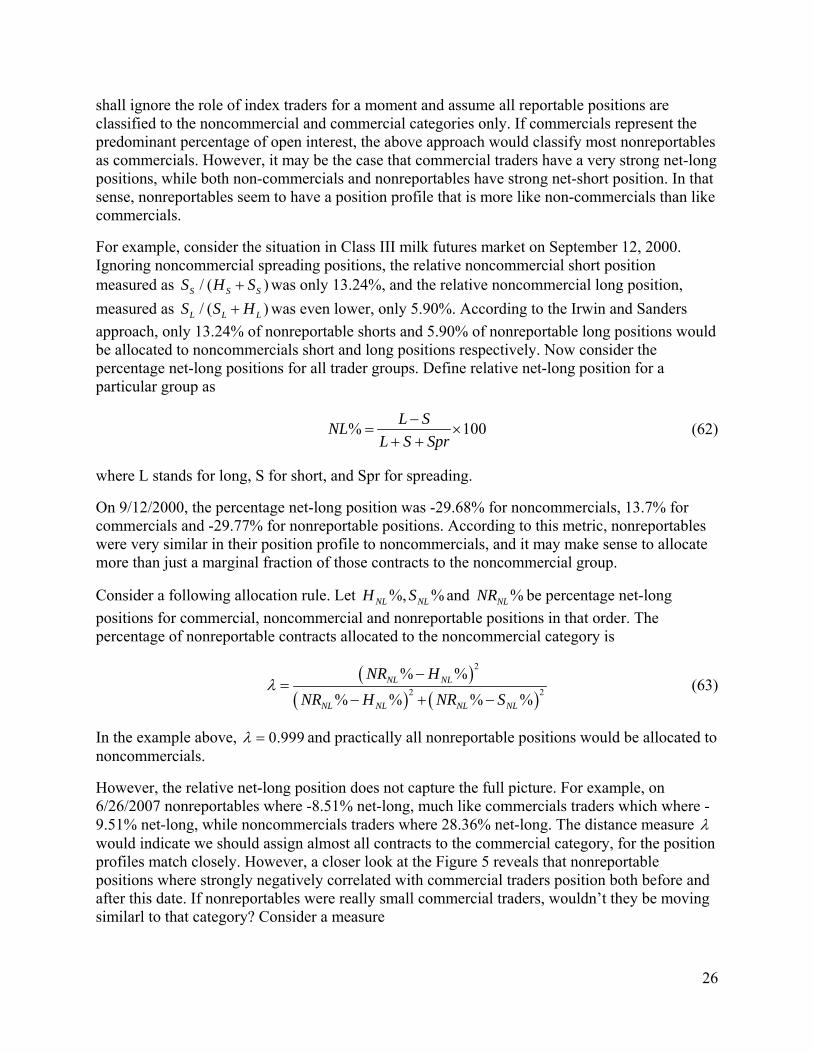
26

shall ignore the role of index traders for a moment and assume all reportable positions are classified to the noncommercial and commercial categories only. If commercials represent the predominant percentage of open interest, the above approach would classify most nonreportables as commercials. However, it may be the case that commercial traders have a very strong net-long positions, while both non-commercials and nonreportables have strong net-short position. In that sense, nonreportables seem to have a position profile that is more like non-commercials than like commercials.

For example, consider the situation in Class III milk futures market on September 12, 2000. Ignoring noncommercial spreading positions, the relative noncommercial short position measured as / ( )S S SS H S was only 13.24%, and the relative noncommercial long position,

measured as / ( )L L LS S H was even lower, only 5.90%. According to the Irwin and Sanders

approach, only 13.24% of nonreportable shorts and 5.90% of nonreportable long positions would be allocated to noncommercials short and long positions respectively. Now consider the percentage net-long positions for all trader groups. Define relative net-long position for a particular group as

% 100L S

NLL S Spr

(62)

where L stands for long, S for short, and Spr for spreading.

On 9/12/2000, the percentage net-long position was -29.68% for noncommercials, 13.7% for commercials and -29.77% for nonreportable positions. According to this metric, nonreportables were very similar in their position profile to noncommercials, and it may make sense to allocate more than just a marginal fraction of those contracts to the noncommercial group.

Consider a following allocation rule. Let %, %NL NLH S and %NLNR be percentage net-long

positions for commercial, noncommercial and nonreportable positions in that order. The percentage of nonreportable contracts allocated to the noncommercial category is

2

2 2

% %

% % % %NL NL

NL NL NL NL

NR H

NR H NR S

(63)

In the example above, 0.999 and practically all nonreportable positions would be allocated to noncommercials.

However, the relative net-long position does not capture the full picture. For example, on 6/26/2007 nonreportables where -8.51% net-long, much like commercials traders which where -9.51% net-long, while noncommercials traders where 28.36% net-long. The distance measure would indicate we should assign almost all contracts to the commercial category, for the position profiles match closely. However, a closer look at the Figure 5 reveals that nonreportable positions where strongly negatively correlated with commercial traders position both before and after this date. If nonreportables were really small commercial traders, wouldn’t they be moving similarl to that category? Consider a measure

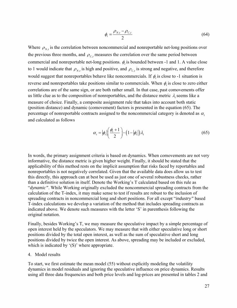
27

, ,

2N t C t

t

(64)

Where ,N t is the correlation between noncommercial and nonreportable net-long positions over

the previous three months, and ,C t measures the correlation over the same period between

commercial and nonreportable net-long positions. t is bounded between -1 and 1. A value close

to 1 would indicate that ,N t is high and positive, and ,C t is strong and negative, and therefore

would suggest that nonreportables behave like noncommercials. If t is close to -1 situation is

reverse and nonreportables take positions similar to commercials. When t is close to zero either

correlations are of the same sign, or are both rather small. In that case, past comovements offer us little clue as to the composition of nonreportables, and the distance metric t seems like a

measure of choice. Finally, a composite assignment rule that takes into account both static (position distance) and dynamic (comovement) factors is presented in the equation (65). The percentage of nonreportable contracts assigned to the noncommercial category is denoted as tand calculated as follows

11

2t

t t t t

(65)

In words, the primary assignment criteria is based on dynamics. When comovements are not very informative, the distance metric is given higher weight. Finally, it should be stated that the applicability of this method rests on the implicit assumption that risks faced by reportables and nonreportables is not negatively correlated. Given that the available data does allow us to test this directly, this approach can at best be used as just one of several robustness checks, rather than a definitive solution in itself. Denote the Working’s T calculated based on this rule as “dynamic”. While Working originally excluded the noncommercial spreading contracts from the calculation of the T-index, it may make sense to test if results are robust to the inclusion of spreading contracts in noncommercial long and short positions. For all except “industry” based T-index calculations we develop a variation of the method that includes spreading contracts as indicated above. We denote such measures with the letter ‘S’ in parenthesis following the original notation.

Finally, besides Working’s T, we may measure the speculative impact by a simple percentage of open interest held by the speculators. We may measure that with either speculative long or short positions divided by the total open interest, as well as the sum of speculative short and long positions divided by twice the open interest. As above, spreading may be included or excluded, which is indicated by ‘(S)’ where appropriate.

4. Model results

To start, we first estimate the mean model (55) without explicitly modeling the volatility dynamics in model residuals and ignoring the speculative influence on price dynamics. Results using all three data frequencies and both price levels and log-prices are presented in tables 2 and

28

3. Results are consistent and suggest that short-term dynamics in cash prices do not influence the direction of futures prices. Futures prices seem to have one-day momentum dynamics as the coefficient of differenced futures prices lagged once is significant. In both model specifications cash prices adjust to the cash-futures spread. However, weak evidence of futures prices adjusting to the spread is found only when using publicly reported closing cash prices that may be bids or offers (not transactions), and that seems to be the only observable difference between the model specifications. It seems that the data frequency only influences the magnitude of the spread coefficient in the cash equation. The coefficient is -0.068 for daily frequency and -0.33 for weekly frequency. The relative magnitude closely resembles the change in frequency – one week contains 5 trading days, and the coefficient in the weekly equation is about 5 times as big as the one in the model estimated using daily frequency.

The next topic of interest includes the volatility spillovers between cash and futures markets. We estimate the standard BEKK model using weekly frequency and price data in levels. Results are reported in Table 3. Several results are interesting. First, when the mean model was estimated without a specified variance structure, we found very little evidence that futures prices adjust to the spread between cash and futures. That adjustment coefficient is now found to be significant. Next, we find that volatility spillovers are bidirectional. Coefficients 21 and 21 capture the

spillovers from futures to cash markets. We see that both coefficients are negative, although only

21 is significant. To measure the sign of an average impact of these spillovers, we calculate the

share of the cash conditional variance attributable to futures for each observation, and take an average. We find that on average, volatility spillovers are negative. Estimating the model for cash data that include unfilled bids and uncovered offers, we find that this result is reversed and that volatility spillovers are positive. While this analysis is preliminary, and robustness of these results needs to be further checked, it is interesting to consider what this would really mean in practice. Cash markets for cheese are very thin, and not more than a handful of sales occur per one trading session, and often it is the case that no sales happen. This result could indicate that in turbulent times price discovery in cash markets is done via bids/offers, while sales are few. That would make sense, since this is a surplus market. In thin markets, an agent that is one of the few sellers with a surplus of cheese to sell and believes that price will continue to increase is likely to wait and try to capture a better price in one of the following trading sessions. A recent Government Accountability Office study (2007) of the cheese spot market brings further examples that fit well with this story:

“Between January 1, 1999, and February 2, 2007, the closing price for block cheese fluctuated based on unfilled bids and uncovered offers on at least 17 percent of the trading days. During the same time period, the barrel market closing price fluctuated based on unfilled bids and uncovered offers 28 percent of trading days.

• Between March 1, 2004, and April 16, 2004, block cheese prices increased from $1.49 to $2.20 per pound, or 48 percent, on the CME spot cheese market based primarily on unfilled bids to buy cheese, with only four carloads of block cheese bought or sold during this period.

• Between October 26, 2004, and November 19, 2004, block cheese prices rose from $1.57 to $1.80 per pound, or 14 percent, with completed transactions for only three carloads of cheese completed during this period."

29

In conclusion, my reading of these results is that higher volatility in the futures market translates to higher volatility in cash market if we look at closing prices that may be bids or offer quotes. But when it comes to sales prices, they are less likely to follow as fast, and sales cash forecast variance declines in times of high volatility in the futures.

Finally, we estimate the full model (55)-(57). We have estimated four variations of the model. Model 1 imposes restriction (58), i.e. effects of additional regressors does not enter the GARCH structure in the subsequent period, while Model 2 allows such effects to be present as in equation (56). For both model versions, we first allow the conditional correlation to be directly impacted by speculators, and check if the conditional covariance matrix was positive definite at each data point after the estimation is completed. Results from estimation that insures positive definiteness of the covariance matrix ex ante by restricting correlation via (59) are also presented. To further check robustness of the results, we estimate the model for 14 alternative measures of speculative influence described in the previous section. It needs to be noted that these robustness checks cannot completely compensate for the potential measurement errors that can arise from the fact that imputed, rather than observed cheese futures prices were used prior to July 2010.

Results, presented in Table 4, reveal that Working’s T index in the Class III milk futures are on average much lower than any of the twelve agricultural futures markets analyzed recently by Irwin and Sanders (2010). For example, they find that average T-index for corn was 1.15, 1.17 in soybeans, 1.44 in CBOT wheat, 1.86 in feeder cattle, and 1.14 in cocoa. Using their method, we find that T-index is only 1.03 in the class III milk futures. My alternative calculations based on dynamics of nonreportable positions bring the T-index up to 1.10, and in fact the theoretical upper bound obtained by allocating all of the nonreportables to noncommercial traders is 1.16. Irwin and Sanders state that value of 1.15 would be historically considered an inadequate amount of speculation to efficiently meet hedging demands and facilitate the transfer of risk.

We find that Model 1 with unrestricted correlation almost always fails to converge. Overall, the highest likelihood is obtained using variation 2 of the model with unrestricted conditional correlations. In each case the conditional covariance is found to be positive definite for all observations. In most specifications, likelihood ratio test rejects restricted correlation version of model 2 in favor of unrestricted correlationFor conditional variance of the futures price, coefficients of speculative adequacy are always either negative or not statistically significantly different from zero. This constitutes strong evidence that there is no excessive speculation in the Class III milk prices. In fact, according to standards suggested by Irwin and Sanders (2010), it could be that speculation in Class III milk futures market is inadequate. My current results indicate that on a weekly frequency, more noncommercial presence would predict lower conditional variance of the futures prices.

5. Conclusions and directions for future research

The task of this essay was to examine price discovery, volatility spillovers and impacts of speculation in the dairy sector. We have developed a method that allows for the calculation of implied cheese futures prices for a period before cheese futures actually started trading. Evidence for periods when cheese futures did trade suggests that utilized approximation methods perform very well. Examining the time series properties of cheese cash and implied futures price we find

30

that the unit root hypothesis is strongly rejected for cash prices, while unit roots cannot be rejected for nearby futures prices in the framework that carefully controls for rollovers. To explain this result, we built a model that illustrates the time series properties of the nearby futures price series for a futures contract written on a second-order stationary cash series and identified the mean-reverting nonlinear dynamics that will occur at rollovers. Given the time series properties of the cash and futures series we propose an error-correction model using spreads between cash and the second nearby futures instead of the cointegration vector. To account for volatility dynamics we employ the GARCH-BEKK structure. We find that the flow of information in the mean model is predominantly from futures to cash, while volatility spillovers are bidirectional. It is possible that cash prices that include unfilled bid/offers react differently to increases in volatility in futures prices than sales cash prices, though this result may not be robust and further research is needed to identify if liquidity in the cash market is reduced with increase in conditional volatility of the futures price. We propose an extension of the BEKK variance model that we refer to as GARCH-MEX. That model does not restrict the sign of the additional regressors on the conditional variances, and can easily insure positive-definiteness of the conditional covariance matrix. Utilizing that model to evaluate the impact of speculation we find strong evidence against the hypothesis that excessive speculation is increasing the conditional variance of futures prices. If anything, speculation may in fact be inadequate, and further research with daily speculative positions and high-frequency futures prices is needed to identify the effect of increased speculation on realized volatility of futures prices, bid-ask spread and magnitude of slippage.

Strong desirability of higher liquidity is clearly seen in the dairy futures products. CME offers seven dairy futures products, but Class III milk has by far the highest open interest, volume and is probably the only dairy futures market to attract speculative interest. While processors hedge their input prices with class III milk, most dairy farmers are interested in protecting their milk mailbox prices which depend on both Class III and Class IV futures prices. In fact, in the second quarter of 2011, the minimum price of fluid milk was calculated using Advanced Class IV, not Class III milk prices. However, Class IV milk futures did not attract significant additional volume, and Class III milk futures remain the center for price risk transfer. Several dairy groups have recently proposed legislative measures that would simplify milk pricing. From a price risk management point of view, simplifying the milk pricing process could enhance the price discovery role of the futures prices, bring new hedging interest to the futures contract and consequently attract more speculative capital. My results indicate more speculative presence could lead to a more stable futures market.

The finding of bidirectional volatility spillovers could indicate that cash prices do also help discover the price levels in the futures market. However, since the cash market trades for only ten minutes in the morning, if the new information is incorporated in the futures market by the end of the day, then a model that uses only daily closing data will fail to uncover the information transmission arising from lagged cash price, as the information flow occurs at a higher frequency. However, this market setting can also be turned to a researcher’s advantage. Given that the cash market is open for only short periods of time each day makes it rather easy to uncover information flows from cash to futures if high-frequency futures prices are used. For example, one dairy broker (Schalla, 2011) summarized in his blog the events of one particularly turbulent day in the cheese markets, following several weeks of increases in cheese blocks prices on the spot market, mostly on unfilled bids and with little or no sales transactions:

31

“9:05 a.m. – July Milk opens the day trading session at $20.13/cwt., off 4 cents from the day before.

10:45 a.m. – Heading into the daily cash cheese session, July drops a minimal 4 cents from the open to $20.09.

10:48 a.m. – Cash cheese session closes with no action seen in either the Block or Barrel market. This spooks the milk market, and the July contract free-falls to $19.87, 22 cents lower than just three minutes earlier.”

By focusing on activity of the futures markets immediately after the close of the cash market we can identify the information contribution of the cash market. Should we find it to be substantial, that will be an additional cause for worry. The CME cash market is very thin, and agents trading on this market may exhibit market power that is inconsistent with perfect competition that agricultural cash markets are usually taken to be. A previous study of the National Cheese Exchange (NCE) undertaken by Mueller et al. (1996) found the presence of cash price manipulation. Shortly afterwards NCE was closed and cheese spot trading moved to the Chicago Board of Trade. While a recent GAO (2007) study indicates that safeguards against market manipulation are stronger at CBOT than they were at the NCE, further analytical study of cash market behavior is needed.

In conclusion, while the specifics of milk pricing, the nature of milk production, and the thinness of cash and futures cheese markets presented me with interesting challenges in evaluating the market characteristics, the overall conclusion is actually quite simple – effective price discovery needs deep and liquid futures as well as cash markets. Any proposed policy change should be evaluated by its potential to simplify and deepen market based price discovery and risk management. If there is any excessive volatility in milk prices, it is more likely to be a consequence of overregulation which leads to fragmented and thin markets, rather than animal spirits of profit-seeking speculators.

32

References

Bessler, D. A. and T. Covey (1991). Cointegration: Some results on U.S. cattle prices. The Journal of Futures Markets 11 (4), 461-474.

Bhar, R. (2001). Return and volatility dynamics in the spot and futures markets in Australia: An intervention analysis in a bivariate EGARCH-x framework. The Journal of Futures Markets 21 (9), 833-850.

Bhar, R. and B. Nikolova (2009). Return, volatility spillovers and dynamic correlation in the BRIC equity markets: An analysis using a bivariate EGARCH framework. Global Finance Journal 19 (3), 203-218.

Brockman, P. and Y. Tse (1995). Information shares in canadian agricultural cash and futures markets. Applied Economics Letters 2, 335-338.

Brorsen, B. W., C. M. Oellermann, and P. L. Farris (1989). The live cattle futures market and daily cash price movements. The Journal of Futures Markets 9 (4), 273-282.

Brunetti, C. and B. Büyükşahin (2009). Is speculation destabilizing? Working Paper, Available from URL: http://papers.ssrn.com/sol3/papers.cfm?abstract_id=1393524 [accessed 25 June, 2011]

Brunetti, C., B. Büyükşahin, and J. H. Harris (2011). Speculators, prices and market volatility. Working Paper, Available from URL: http://papers.ssrn.com/sol3/papers.cfm?abstract_id=1736737 [accessed 25 June, 2011]

Büyükşahin, B. and M. A. Robe (2011). Speculators, commodities and Cross-Market linkages. Working Paper, Available from URL: http://papers.ssrn.com/sol3/papers.cfm?abstract_id=1707103 [accessed 25 June, 2011]

Cheung, Y. and L. K. Ng (1996). A causality-in-variance test and its application to financial market prices. Journal of Econometrics 72 (1-2), 33-48.

Comte, F. and O. Lieberman (2000). Second-Order noncausality in multivariate GARCH processes. Journal of Time Series Analysis 21 (5), 535-557.

Comte, F. and O. Lieberman (2003). Asymptotic theory for multivariate GARCH processes. Journal of Multivariate Analysis 84 (1), 61-84.

Cox, C. C. (1976). Futures trading and market information. The Journal of Political Economy 84 (6), 1215-1237.

Dickey, D. A. and W. A. Fuller (1979). Distribution of the estimators for autoregressive time series with a unit root. Journal of the American Statistical Association 74 (366), 427-431.

Du, X., C. L. Yu, and D. J. Hayes (2011). Speculation and volatility spillover in the crude oil and agricultural commodity markets: A Bayesian analysis. Energy Economics 33 (3), 497-503.

33

Fortenbery, T. R. and H. O. Zapata (1993). An examination of cointegration relations between futures and local grain markets. The Journal of Futures Markets 13 (8), 921-932.

Fortenbery, T. R. and H. O. Zapata (1997). An evaluation of price linkages between futures and cash markets for cheddar cheese. The Journal of Futures Markets 17 (3), 279-301.

Fortenbery, T. R., R. A. Cropp, and H. Zapata (1997). Analysis of expected price dynamics between fluid milk futures contracts and cash prices for fluid milk. Journal of Agribusiness 15 (2), 215-234.

Fortenbery, T. R. and H. O. Zapata (2004). Developed speculation and underdeveloped markets – the role of futures trading on export prices in less developed countries. European Review of Agricultural Economics 31 (4), 451-471.

GAO (2007). Spot Cheese Market - Market oversight has increased, but concerns remain about potential manipulation. Technical report. U.S. Government Accountability Ofice.

Garbade, K. D. and W. L. Silber (1983). Price movements and price discovery in futures and cash markets. The Review of Economics and Statistics 65 (2), 289-297.

Geweke, J. and S. Porter-Hudak (1983). The estimation and application of long memory time series models. Journal of Time Series Analysis 4 (4), 221-238.

Gilbert, C. L. (2010). How to understand high food prices. Journal of Agricultural Economics 61 (2), 398-425.

Granger, C. W. J. (1980). Testing for causality: A personal viewpoint. Journal of Economic Dynamics and Control 2 (2-4), 329-352.

Granger, C. W. J., R. P. Robins, and R. F. Engle (1986). Wholesale and Retail Prices: Bivariate Time-Series Modeling with Forecastable Error Variances in Model Reliability (eds. David Belsley and Edwin Kuh), pp. 1-16. Cambridge, MA: The MIT Press.

Gray, R. W. (1963). Onions revisited. Journal of Farm Economics 45 (2), 273-276.

Hamilton, J. D. (2009). Causes and consequences of the oil shock of 2007–08. Brookings Papers on Economic Activity, (Spring), 215-261.

Hansen, L. P. and T. J. Sargent (1980). Formulating and estimating dynamic linear rational expectations models. Journal of Economic Dynamics and Control 2, 7-46.

Irwin, S. H., D. R. Sanders, and R. P. Merrin (2009). Devil or angel? the role of speculation in the recent commodity price boom (and bust). Journal of Agricultural and Applied Economics 41 (2), 377-391.

Irwin, S. H. and D. R. Sanders (2010). The impact of index and swap funds on commodity futures Markets: Preliminary results. OECD Food, Agriculture and Fisheries Working Papers 27, OECD Publishing.

Ivanov, S. and J. H. Cho (2011). A study of the factors affecting price discovery in commodity markets. Proceedings of the 2011 Southwestern Finance Association Conference, Available at

34

URL: http://www.southwesternfinance.org/conf-2011/swfa2011_submission_24.pdf [accessed 25 June, 2011]

Johansen, S. and K. Juselius (1990). Maximum likelihood estimation and inference on cointegration - with applications to the demand for money. Oxford Bulletin of Economics and Statistics 52 (2), 169-210.

Koutmos, G. and M. Tucker (1996). Temporal relationships and dynamic interactions between spot and futures stock markets. The Journal of Futures Markets 16 (1), 55-69.

Ling, S. and M. McAleer (2003). Asymptotic theory for a vector ARMA-GARCH model. Econometric Theory 19 (02), 280-310.

Masters, M. W. (2008). Testimony before the commodity futures trading commission. May 20, 2008. Accessed from URL: http://hsgac.senate.gov/public/_files/052008Masters.pdf. [accessed June 25, 2011]

Mattos, F. and P. Garcia (2006). Identifying price discovery and risk transfer in thinly traded markets: Evidence from Brazilian agricultural futures markets. The Review of Futures Markets 14 (4), 469-480.

Mueller, W. F., B. W. Marion, M. H. Sial, and F. E. Geithman (1996, March). Cheese pricing: A study of the National Cheese Exchange. Technical report, Deparment of Agricultural Economics, University of Wisconsin-Madison, Madison, WI.

Nelson, D. B. (1991). Conditional heteroskedasticity in asset returns: A new approach. Econometrica 59 (2), 347-370.

Newbery, D. M. (1987). When do futures destabilize spot prices? International Economic Review 28 (2), 291-297.

Oellermann, C. M. and P. L. Farris (1985). Futures or cash: Which market leads live beef cattle prices? The Journal of Futures Markets 5 (4), 529-538.

Peck, A. E. (1980). The role of economic analysis in futures market regulation. American Journal of Agricultural Economics 62 (5), 1037-1043.

Phillips, P. C. B. and P. Perron (1988). Testing for a unit root in time series regression. Biometrika 75 (2).

Powers, M. J. (1970). Does futures trading reduce price fluctuations in the cash markets? The American Economic Review 60 (3), 460-464.

Rutledge, D. J. S. (1977). Estimation of hedging and speculative positions in futures markets - an alternative approach. Food Research Institute Studies 16 (3), 205-211.

Said, S. E. and D. A. Dickey (1984). Testing for unit roots in autoregressive-moving average models of unknown order. Biometrika 71 (3), 599-607.

35

Sanders, D. R., S. H. Irwin, and R. P. Merrin (2010). The adequacy of speculation in agricultural futures markets: Too much of a good thing? Applied Economic Perspectives and Policy 32 (1), 77-94.

Schalla, S. (2011). Control the emotions and impulsive decisions that milk market volatility can produce. Available at URL: http://www.agweb.com/livestock/dairy/blog/Know_Your_Market_281/?Year=2011&Month=6. [accessed 25 June, 2011]

Schroeder, T. C. and B. K. Goodwin (1991). Price discovery and cointegration for live hogs. The Journal of Futures Markets 11 (6), 685-696.

Streeter, D. H. and W. G. Tomek (1992). Variability in soybean futures prices: An integrated framework. The Journal of Futures Markets 12 (6), 705-728.

Tang, K. and W. Xiong (2010). Index investment and financialization of commodities. NBER Working Paper No. 16835. Available from URL: http://www.nber.org/papers/w16385 [accessed 25 June, 2011]

Taylor, G. S. and R. M. Leuthold (1974). The influence of futures trading on cash cattle price variations. Food Research Institute Studies 13 (1), 29-35.

Thraen, C. S. (1999). A note: The CSCE cheddar cheese cash and futures price long-term equilibrium relationship revisited. The Journal of Futures Markets 19(2), 233-244.

Wang, D. and W. G. Tomek (2007). Commodity prices and unit root tests. American Journal of Agricultural Economics 89 (4), 873-889.

Wold, H. (1954). A Study in the Analysis of Stationary Time Series. Almqvist & Wiksell.

Turnovsky, S. J. (1983). The determination of spot and futures prices with storable commodities. Econometrica 51 (5), 1363-1387.

Tse, Y. (1999). Price discovery and volatility spillovers in the DJIA index and futures markets. The Journal of Futures Markets 19 (8), 911-930.

Yang, J., D. A. Bessler, and D. J. Leatham (2001). Asset storability and price discovery in commodity futures markets: A new look. The Journal of Futures Markets 21 (3), 279-300.

Witherspoon, J. T. (1993). How price discovery by futures impacts the cash market. The Journal of Futures Markets 13 (5), 469-496.

Working, H. (1960, Feb). Price effects of futures trading. Food Research Institute Studies 1 (1), 3-31.

Working, H. (1960, May). Speculation on hedging markets. Food Research Institute Studies 1 (2), 185-220.

Working, H. (1962). New concepts concerning futures markets and prices. The American Economic Review 52 (3), 431-459.

36

Zapata, H. O. and T. R. Fortenbery (1996). Stochastic interest rates and price discovery in selected commodity markets. Review of Agricultural Economics 18, 643-654.

Zhong, M., A. Darrat, and R. Otero (2004). Price discovery and volatility spillovers in index futures markets: Some evidence from Mexico. Journal of Banking & Finance 28 (12), 3037-3054.

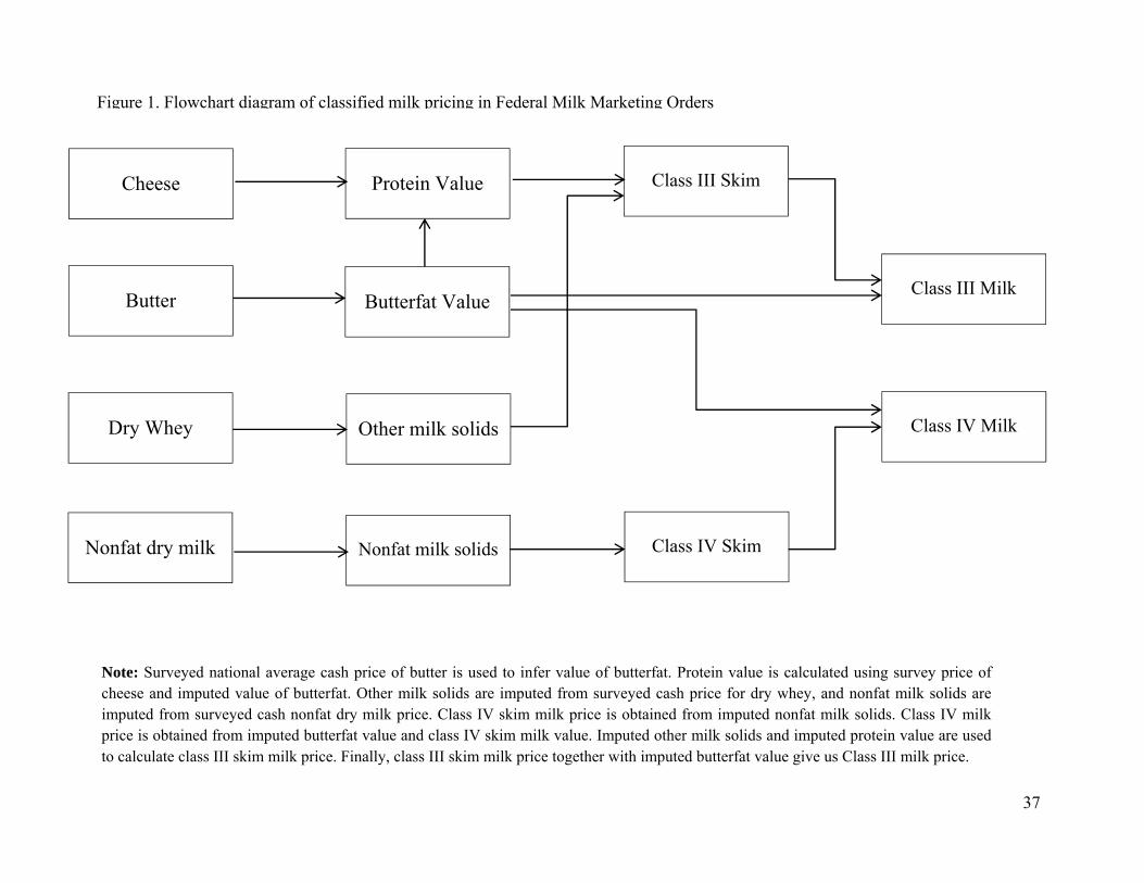
37

Cheese

Butter

Dry Whey

Nonfat dry milk

Protein Value

Butterfat Value

Other milk solids

Nonfat milk solids

Class III Skim

Class IV Skim

Class III Milk

Class IV Milk

Note: Surveyed national average cash price of butter is used to infer value of butterfat. Protein value is calculated using survey price of cheese and imputed value of butterfat. Other milk solids are imputed from surveyed cash price for dry whey, and nonfat milk solids are imputed from surveyed cash nonfat dry milk price. Class IV skim milk price is obtained from imputed nonfat milk solids. Class IV milk price is obtained from imputed butterfat value and class IV skim milk value. Imputed other milk solids and imputed protein value are used to calculate class III skim milk price. Finally, class III skim milk price together with imputed butterfat value give us Class III milk price.

Figure 1. Flowchart diagram of classified milk pricing in Federal Milk Marketing Orders

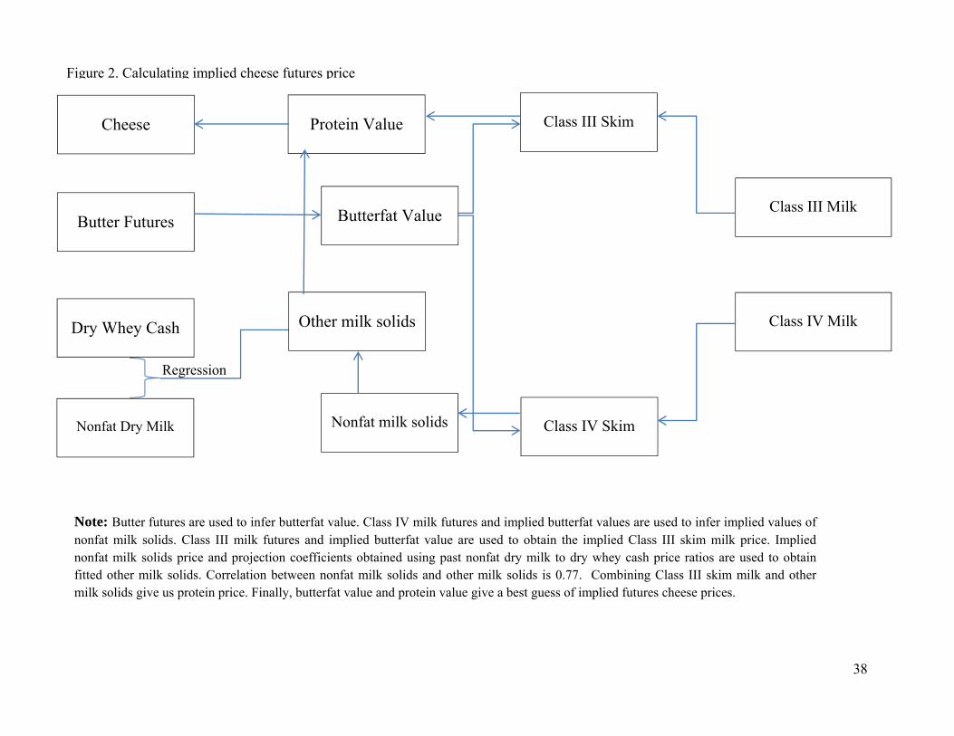
38

 

 

 

 

Cheese

Butter Futures

Dry Whey Cash

Nonfat Dry Milk

Protein Value

Nonfat milk solids

Class III Skim

Class IV Skim

Class III Milk

Class IV Milk

Regression

Note: Butter futures are used to infer butterfat value. Class IV milk futures and implied butterfat values are used to infer implied values of nonfat milk solids. Class III milk futures and implied butterfat value are used to obtain the implied Class III skim milk price. Implied nonfat milk solids price and projection coefficients obtained using past nonfat dry milk to dry whey cash price ratios are used to obtain fitted other milk solids. Correlation between nonfat milk solids and other milk solids is 0.77. Combining Class III skim milk and other milk solids give us protein price. Finally, butterfat value and protein value give a best guess of implied futures cheese prices.

Figure 2. Calculating implied cheese futures price

Butterfat Value

Other milk solids

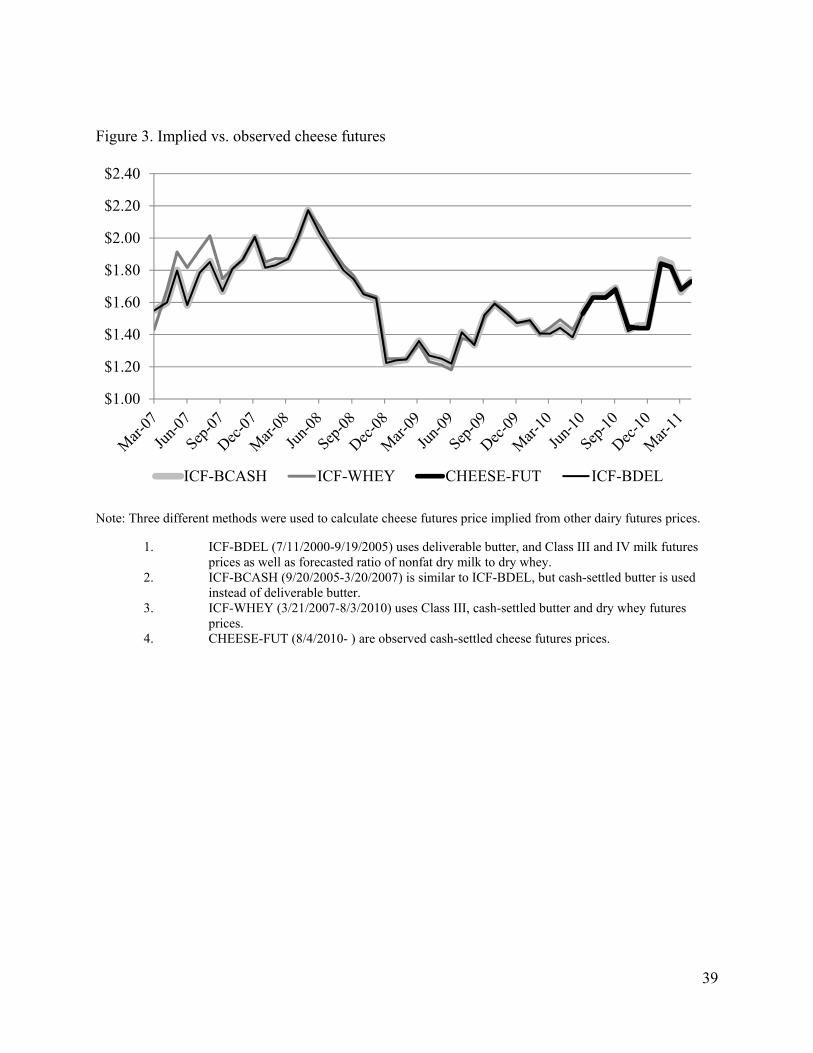
39

 

Figure 3. Implied vs. observed cheese futures

Note: Three different methods were used to calculate cheese futures price implied from other dairy futures prices.

1. ICF-BDEL (7/11/2000-9/19/2005) uses deliverable butter, and Class III and IV milk futures prices as well as forecasted ratio of nonfat dry milk to dry whey.

2. ICF-BCASH (9/20/2005-3/20/2007) is similar to ICF-BDEL, but cash-settled butter is used instead of deliverable butter.

3. ICF-WHEY (3/21/2007-8/3/2010) uses Class III, cash-settled butter and dry whey futures prices.

4. CHEESE-FUT (8/4/2010- ) are observed cash-settled cheese futures prices.

$1.00

$1.20

$1.40

$1.60

$1.80

$2.00

$2.20

$2.40

ICF-BCASH ICF-WHEY CHEESE-FUT ICF-BDEL

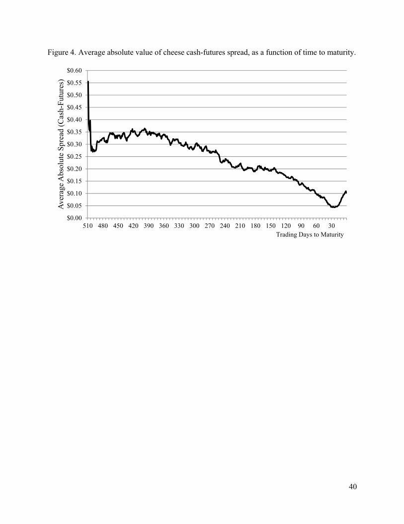
40

Figure 4. Average absolute value of cheese cash-futures spread, as a function of time to maturity.

$0.00

$0.05

$0.10

$0.15

$0.20

$0.25

$0.30

$0.35

$0.40

$0.45

$0.50

$0.55

$0.60

510 480 450 420 390 360 330 300 270 240 210 180 150 120 90 60 30

Ave

rage

Abs

olut

e S

prea

d (C

ash-

Fut

ures

)

Trading Days to Maturity

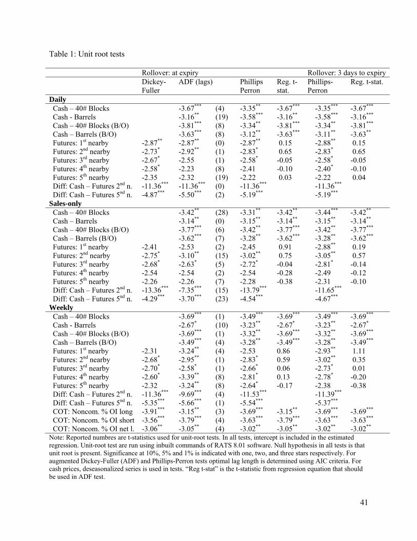
41

Table 1: Unit root tests

Note: Reported numbres are t-statistics used for unit-root tests. In all tests, intercept is included in the estimated regression. Unit-root test are run using inbuilt commands of RATS 8.01 software. Null hypothesis in all tests is that unit root is present. Significance at 10%, 5% and 1% is indicated with one, two, and three stars respectively. For augmented Dickey-Fuller (ADF) and Phillips-Perron tests optimal lag length is determined using AIC criteria. For cash prices, deseasonalized series is used in tests. “Reg t-stat” is the t-statistic from regression equation that should be used in ADF test.

Rollover: at expiry Rollover: 3 days to expiry Dickey-

Fuller ADF (lags) Phillips

Perron Reg. t-stat.

Phillips-Perron

Reg. t-stat.

Daily Cash – 40# Blocks -3.67*** (4) -3.35** -3.67*** -3.35*** -3.67*** Cash - Barrels -3.16** (19) -3.58*** -3.16** -3.58*** -3.16*** Cash – 40# Blocks (B/O) -3.81*** (8) -3.34** -3.81*** -3.34** -3.81*** Cash – Barrels (B/O) -3.63*** (8) -3.12** -3.63*** -3.11** -3.63** Futures: 1st nearby -2.87** -2.87** (0) -2.87** 0.15 -2.88** 0.15 Futures: 2nd nearby -2.73* -2.92** (1) -2.83* 0.65 -2.83* 0.65 Futures: 3rd nearby -2.67* -2.55 (1) -2.58* -0.05 -2.58* -0.05 Futures: 4th nearby -2.58* -2.23 (8) -2.41 -0.10 -2.40* -0.10 Futures: 5th nearby -2.35 -2.32 (19) -2.22 0.03 -2.22 0.04 Diff: Cash – Futures 2nd n. -11.36*** -11.36*** (0) -11.36*** -11.36*** Diff: Cash – Futures 5nd n. -4.87*** -5.50*** (2) -5.19*** -5.19*** Sales-only Cash – 40# Blocks -3.42** (28) -3.31** -3.42** -3.44*** -3.42** Cash – Barrels -3.14** (0) -3.15** -3.14** -3.15** -3.14** Cash – 40# Blocks (B/O) -3.77*** (6) -3.42** -3.77*** -3.42** -3.77*** Cash – Barrels (B/O) -3.62*** (7) -3.28** -3.62*** -3.28** -3.62*** Futures: 1st nearby -2.41 -2.53 (2) -2.45 0.91 -2.88** 0.19 Futures: 2nd nearby -2.75* -3.10** (15) -3.02** 0.75 -3.05** 0.57 Futures: 3rd nearby -2.68* -2.63* (5) -2.72* -0.04 -2.81* -0.14 Futures: 4th nearby -2.54 -2.54 (2) -2.54 -0.28 -2.49 -0.12 Futures: 5th nearby -2.26 -2.26 (7) -2.28 -0.38 -2.31 -0.10 Diff: Cash – Futures 2nd n. -13.36*** -7.35*** (15) -13.79*** -11.65*** Diff: Cash – Futures 5nd n. -4.29*** -3.70*** (23) -4.54*** -4.67*** Weekly Cash – 40# Blocks -3.69*** (1) -3.49*** -3.69*** -3.49*** -3.69*** Cash - Barrels -2.67* (10) -3.23** -2.67* -3.23** -2.67* Cash – 40# Blocks (B/O) -3.69*** (1) -3.32** -3.69*** -3.32** -3.69*** Cash – Barrels (B/O) -3.49*** (4) -3.28** -3.49*** -3.28** -3.49*** Futures: 1st nearby -2.31 -3.24** (4) -2.53 0.86 -2.93** 1.11 Futures: 2nd nearby -2.68* -2.95** (1) -2.83* 0.59 -3.02** 0.35 Futures: 3rd nearby -2.70* -2.58* (1) -2.66* 0.06 -2.73* 0.01 Futures: 4th nearby -2.60* -3.39** (8) -2.81* 0.13 -2.78* -0.20 Futures: 5th nearby -2.32 -3.24** (8) -2.64* -0.17 -2.38 -0.38 Diff: Cash – Futures 2nd n. -11.36*** -9.69*** (4) -11.53*** -11.39*** Diff: Cash – Futures 5nd n. -5.35*** -5.66*** (1) -5.54*** -5.37*** COT: Noncom. % OI long -3.91*** -3.15** (3) -3.69*** -3.15** -3.69*** -3.69*** COT: Noncom. % OI short -3.56*** -3.79*** (4) -3.63*** -3.79*** -3.63*** -3.63*** COT: Noncom. % OI net l. -3.06** -3.05** (4) -3.02** -3.05** -3.02** -3.02**

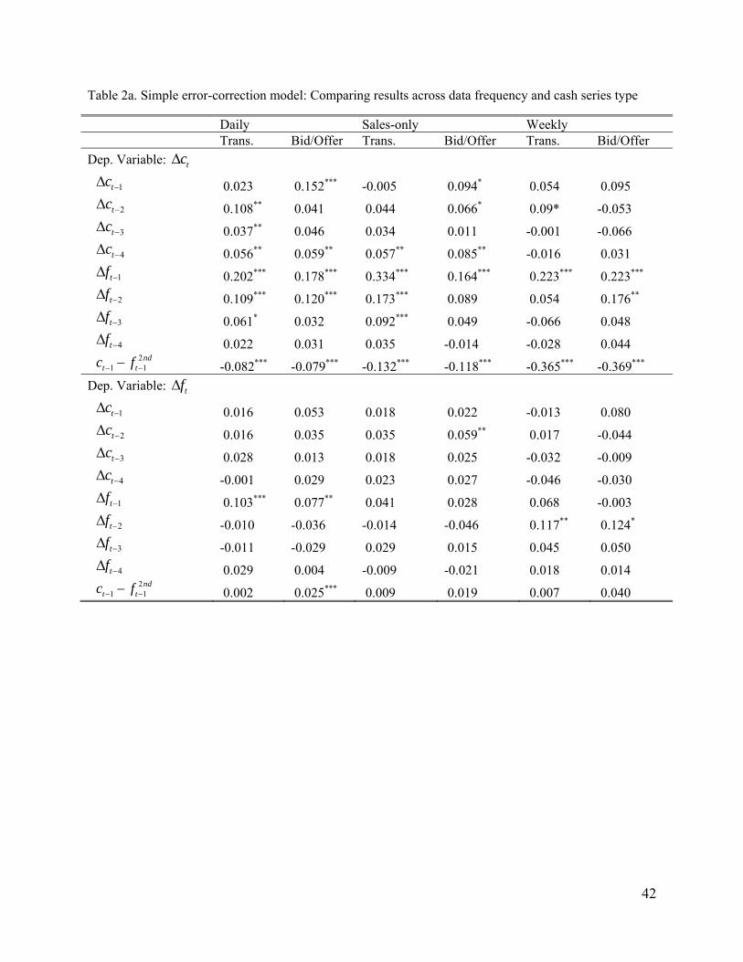
42

Table 2a. Simple error-correction model: Comparing results across data frequency and cash series type

Daily Sales-only Weekly Trans. Bid/Offer Trans. Bid/Offer Trans. Bid/Offer

Dep. Variable: tc

1tc 0.023 0.152*** -0.005 0.094* 0.054 0.095 2tc 0.108** 0.041 0.044 0.066* 0.09* -0.053 3tc 0.037** 0.046 0.034 0.011 -0.001 -0.066 4tc 0.056** 0.059** 0.057** 0.085** -0.016 0.031 1tf 0.202*** 0.178*** 0.334*** 0.164*** 0.223*** 0.223*** 2tf 0.109*** 0.120*** 0.173*** 0.089 0.054 0.176** 3tf 0.061* 0.032 0.092*** 0.049 -0.066 0.048 4tf 0.022 0.031 0.035 -0.014 -0.028 0.044 2

1 1nd

t tc f -0.082*** -0.079*** -0.132*** -0.118*** -0.365*** -0.369***

Dep. Variable: tf 1tc 0.016 0.053 0.018 0.022 -0.013 0.080 2tc 0.016 0.035 0.035 0.059** 0.017 -0.044 3tc 0.028 0.013 0.018 0.025 -0.032 -0.009

4tc -0.001 0.029 0.023 0.027 -0.046 -0.030 1tf 0.103*** 0.077** 0.041 0.028 0.068 -0.003 2tf -0.010 -0.036 -0.014 -0.046 0.117** 0.124* 3tf -0.011 -0.029 0.029 0.015 0.045 0.050 4tf 0.029 0.004 -0.009 -0.021 0.018 0.014 2

1 1nd

t tc f 0.002 0.025*** 0.009 0.019 0.007 0.040  

 

 

 

 

 

 

 

 

 

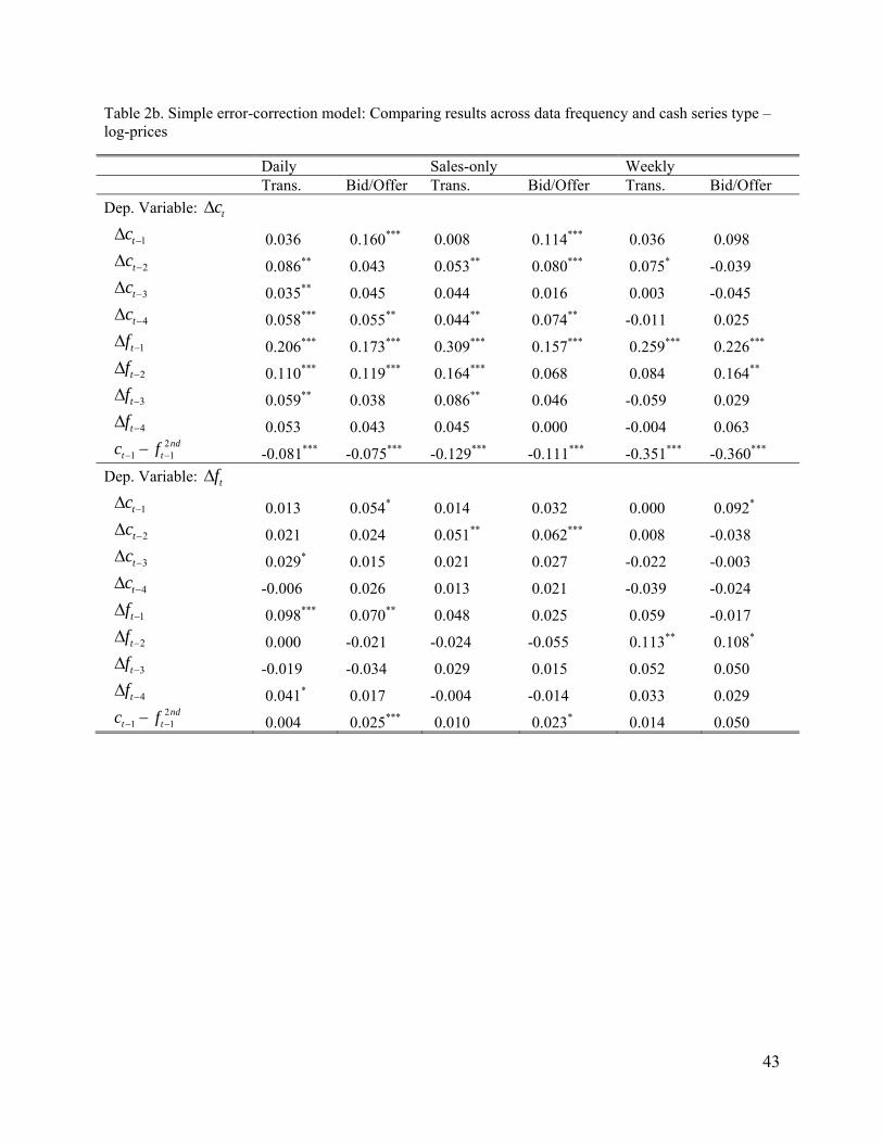
43

Table 2b. Simple error-correction model: Comparing results across data frequency and cash series type – log-prices

Daily Sales-only Weekly Trans. Bid/Offer Trans. Bid/Offer Trans. Bid/Offer

Dep. Variable: tc 1tc 0.036 0.160*** 0.008 0.114*** 0.036 0.098 2tc 0.086** 0.043 0.053** 0.080*** 0.075* -0.039 3tc 0.035** 0.045 0.044 0.016 0.003 -0.045 4tc 0.058*** 0.055** 0.044** 0.074** -0.011 0.025 1tf 0.206*** 0.173*** 0.309*** 0.157*** 0.259*** 0.226*** 2tf 0.110*** 0.119*** 0.164*** 0.068 0.084 0.164** 3tf 0.059** 0.038 0.086** 0.046 -0.059 0.029 4tf 0.053 0.043 0.045 0.000 -0.004 0.063 2

1 1nd

t tc f -0.081*** -0.075*** -0.129*** -0.111*** -0.351*** -0.360***

Dep. Variable: tf 1tc 0.013 0.054* 0.014 0.032 0.000 0.092* 2tc 0.021 0.024 0.051** 0.062*** 0.008 -0.038 3tc 0.029* 0.015 0.021 0.027 -0.022 -0.003

4tc -0.006 0.026 0.013 0.021 -0.039 -0.024 1tf 0.098*** 0.070** 0.048 0.025 0.059 -0.017 2tf 0.000 -0.021 -0.024 -0.055 0.113** 0.108* 3tf -0.019 -0.034 0.029 0.015 0.052 0.050 4tf 0.041* 0.017 -0.004 -0.014 0.033 0.029 2

1 1nd

t tc f 0.004 0.025*** 0.010 0.023* 0.014 0.050  

 

 

 

 

 

 

 

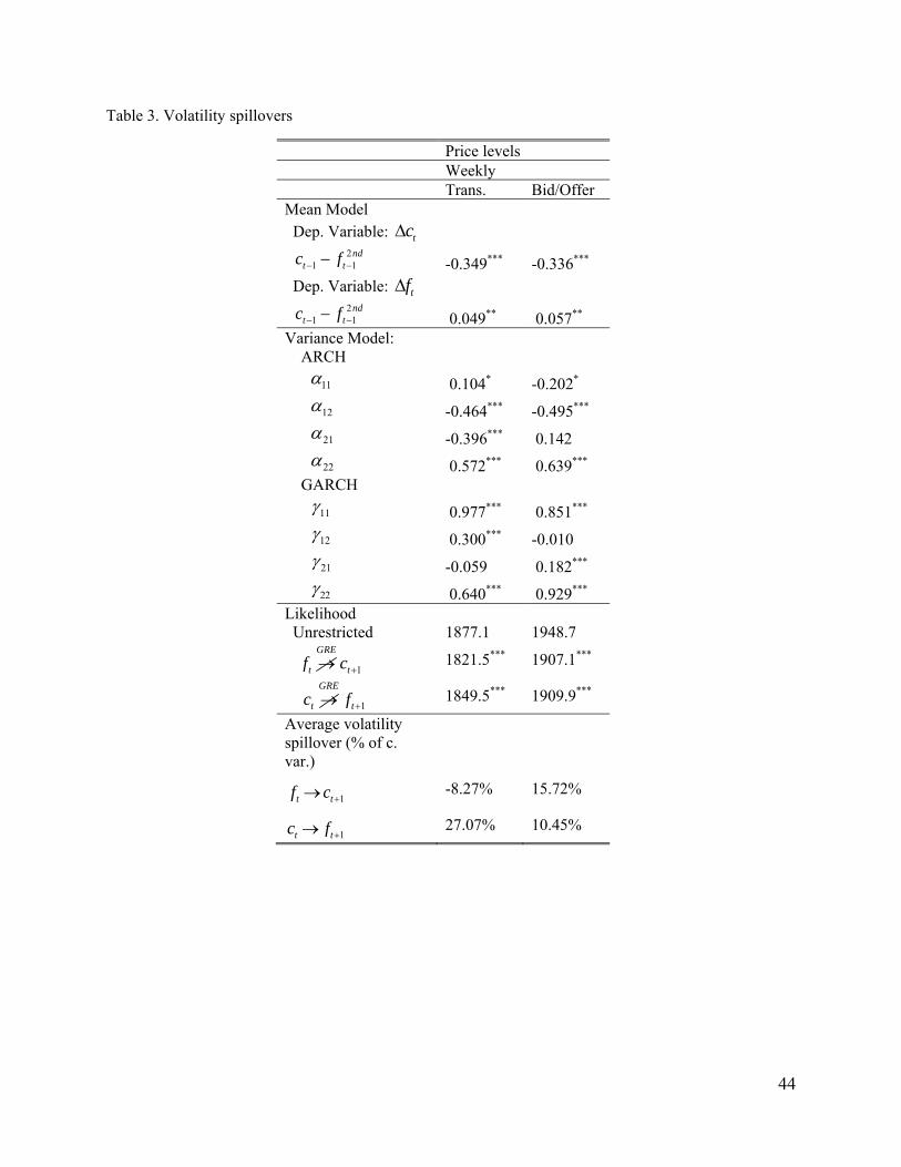
44

Table 3. Volatility spillovers

Price levels Weekly Trans. Bid/Offer Mean Model Dep. Variable: tc 2

1 1nd

t tc f -0.349*** -0.336*** Dep. Variable: tf 2

1 1nd

t tc f 0.049** 0.057** Variance Model: ARCH 11 0.104* -0.202* 12 -0.464*** -0.495*** 21 -0.396*** 0.142 22 0.572*** 0.639*** GARCH 11 0.977*** 0.851*** 12 0.300*** -0.010 21 -0.059 0.182*** 22 0.640*** 0.929*** Likelihood Unrestricted 1877.1 1948.7

1

GRE

t tf c 1821.5*** 1907.1***

1

GRE

t tc f 1849.5*** 1909.9***

Average volatility spillover (% of c. var.)

1t tf c -8.27% 15.72%

1t tc f 27.07% 10.45%

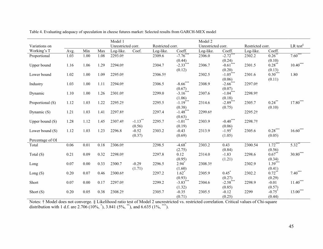
45

Table 4. Evaluating adequacy of speculation in cheese futures market: Selected results from GARCH-MEX model

Model 1 Model 2 Variations on Working’s T

Unrestricted corr. Restricted corr. Unrestricted corr. Restricted corr. LR test§ Avg. Min Max Log-like. Coef. Log-like. Coeff. Log-like. Coeff. Log-like. Coeff.

Proportional 1.03 1.00 1.08 2293.0† 2309.6 -7.76***

(0.44) 2306.0 -2.72***

(0.24) 2302.2 0.26**

(0.10) 7.60***

Upper bound 1.16 1.06 1.29 2294.0† 2304.7 -2.33***

(0.12) 2306.7 -0.61***

(0.20) 2301.5 0.28**

(0.13) 10.40***

Lower bound 1.02 1.00 1.09 2295.0† 2306.5† 2302.5 -1.05***

(0.06) 2301.6 0.30***

(0.11) 1.80

Industry 1.03 1.00 1.11 2294.0† 2306.5 -8.66***

(0.67) 2308.9 -2.66***

(0.07) 2297.0†

Dynamic 1.10 1.00 1.26 2301.0† 2299.0 -3.16***

(1.06) 2307.6 -1.04***

(0.18) 2298.9†

Proportional (S) 1.12 1.03 1.22 2295.2† 2295.5 -1.19*** (0.38)

2314.6 -2.89***

(0.75) 2305.7 0.24**

(0.10) 17.80***

Dynamic (S) 1.21 1.03 1.41 2297.8† 2297.4 -1.48***

(0.63) 2299.6† 2295.2†

Upper bound (S) 1.28 1.12 1.45 2307.4† -1.13**

(0.56) 2295.7 -1.01***

(0.19) 2303.9

-0.40***

(0.06) 2298.7†

Lower bound (S) 1.12 1.03 1.23 2296.8 -0.52 (0.37)

2303.2 -0.43 (0.69)

2313.9 -1.95*

(1.05) 2305.6 0.28***

(0.05) 16.60***

Percentage of OI Total 0.06 0.01 0.18 2306.0† 2298.5 -4.68*

(2.75) 2303.2 0.43

(0.84) 2300.54 1.72***

(0.56) 5.32**

Total (S) 0.21 0.09 0.32 2298.0† 2297.8 0.12 (0.95)

2314.0 -1.83 (1.21)

2298.6 0.67** (0.34)

30.80***

Long 0.07 0.00 0.33 2300.7 -0.29 (1.71)

2296.5 2.94* (1.60)

2308.3† 2302.9 1.39***

(0.41)

Long (S) 0.20 0.07 0.46 2300.6† 2297.2 1.62* (0.93)

2305.9 0.45* (0.27)

2302.2 0.72**

(0.29) 7.40***

Short 0.07 0.00 0.17 2297.0† 2299.2 -3.83***

(1.32) 2304.6 -2.58***

(0.85) 2298.9 -0.01

(0.57) 11.40***

Short (S) 0.20 0.05 0.38 2308.2† 2305.7 -0.35(0.71)

2305.5 -0.12 (0.25)

2299 -0.75*

(0.44) 13.00***

Notes: † Model does not converge. § Likelihood ratio test of Model 2 uncrestricted vs. restricted correlation. Critical values of Chi-square distribution with 1 d.f. are 2.706 (10%, *), 3.841 (5%, **), and 6.635 (1%, ***).