Price Dispersion and Inflation Persistence

Price Dispersion and Inflation Persistence

Takushi Kurozumi and Willem Van Zandweghe

Bank of Japan and FRB Kansas City

SWET 2017August 5, 2017

Disclaimer: The views expressed are those of the authors and should not be interpreted as those of the Bank of Japan, theFederal Reserve Bank of Kansas City, or the Federal Reserve System.

Kurozumi (BOJ) & Van Zandweghe (FRBKC) Price Dispersion & Inflation Persistence SWET 2017 1 / 27

Empirical impulse responses to a monetary policy shock

0 5 10 15 20-0.9

-0.6

-0.3

0

0.3

0.6

pp

Federal Funds Rate

0 5 10 15 20-0.4

-0.2

0

0.2

0.4

pp

Annualized Inflation Rate

0 5 10 15 20

Quarters since shock

-0.6

-0.3

0

0.3

0.6

0.9

%

Output

0 5 10 15 20


-0.6

-0.3

0

0.3

0.6

%

Labor Productivity


Intrinsic or inherited inflation inertia

The New Keynesian Phillips Curve (NKPC) governs inflationdynamics in sticky price models of monetary policy.

NKPC has difficulty accounting for inflation persistence because it ispurely forward-looking, so literature has incorporated lags of inflation.

Intrinsic inflation inertia remains controversial.

Assumptions—rule-of-thumb price setting, price indexation—are oftendeemed implausible.

Benati (2008) finds that the degree of inflation persistence varies withthe monetary policy regime across countries.

To account for inflation persistence without resorting to intrinsicinflation inertia, NKPC must inherit persistence in driving process.


Staggered pricing model with positive trend inflation hasdifficulty generating inflation persistence

Inflation dynamics in generalized NKPC depends on relative pricedistortion (RPD), reflects productivity loss due to price dispersion.

Price dispersion → demand dispersion → RPD.

Lagged RPD is an endogenous state variable, potential source ofpersistence.

However, we find the inertia of RPD has a minor effect on inflationpersistence, while it may generate a counterfactual decline in outputper hour after an expansionary shock.

⇒ Dynamics of RPD creates tension between generating plausibleresponses of inflation and output per hour.


A “smoothed-off” kink in demand curves alters therelationship between price dispersion and RPD

-100 -50 50 100Relative demand (%)

-10

-5

5

10Relative price (%)

θ=10, ϵ=0

θ=10, ϵ=-9

Generalization of Dixit-Stiglitz preferences for product diversity(Kimball, 1995; Smets and Wouters, 2007).

Kink generates strategic complementarity: large demand loss for highrelative price and small demand gain for low relative price.


Responses of inflation and output per hour consistent withVAR evidence

The kink introduces measure of price dispersion, distinct from RPD,which appears in NKPC.

Lagged price dispersion is a second endogenous state variable.

A policy shock generates a large and persistent response of pricedispersion and a muted response of RPD, allowing plausible responsesof both inflation and output per hour.

⇒ Large, persistent response of price dispersion is inherited by theresponse of inflation, which becomes persistent and hump-shaped.

⇒ Muted response of RPD prevents a counterfactual decline of outputper hour.


Credible permanent disinflation

With intrinsic inflation inertia, a permanent decline in trend inflationgenerates a gradual decline in inflation and a recession.

Without the inertia inflation jumps to its new trend rate and outputnever deviates from its trend level.

In our model with trend inflation and a kink in demand curves, acredible disinflation induces a gradual decline in inflation and arecession even absent intrinsic inflation inertia.


Overview

1 Model

2 Quantitative analysis

3 Conclusion


A model with trend inflation and kinked demand curves

Representative final-good producer combines differentiated goods intoa single product according to household preferences.

Curvature in demand curves for differentiated goods.

Continuum of monopolistically competitive intermediate-goodproducers face Calvo price rigidity.

Fixed cost of production gives rise to increasing returns to scale.

Monetary authority conducts interest rate policy and has positiveinflation target.

Representative household.


Representative final-good firm

Following Dotsey & King (2005), demand for differentiated good f is

Yt(f ) =Yt

1 + ε

[(Pt(f )

Ptdt

)−θ(1+ε)

+ ε

].

Parameter ε ≤ 0 governs curvature, which is measured as −εθ, and

dt =

[∫ 1

0(Pt(f )/Pt)

1−θ(1+ε) df

] 11−θ(1+ε)

is a measure of price dispersion.

The case ε = 0 is the familiar CES case:

Demand Yt(f ) = Yt (Pt(f )/Pt)−θ.

Price index Pt = [∫ 1

0(Pt(f ))1−θdf ]1/(1−θ) ⇔ dt = 1.




Yt(f ) =Yt

1 + ε

[(Pt(f )

Ptdt

)−θ(1+ε)

+ ε

].


dt =

[∫ 1

0(Pt(f )/Pt)

1−θ(1+ε) df

] 11−θ(1+ε)





0(Pt(f ))1−θdf ]1/(1−θ) ⇔ dt = 1.




Yt(f ) =Yt

1 + ε

[(Pt(f )

Ptdt

)−θ(1+ε)

+ ε

].


dt =

[∫ 1

0(Pt(f )/Pt)

1−θ(1+ε) df

] 11−θ(1+ε)





0(Pt(f ))1−θdf ]1/(1−θ) ⇔ dt = 1.


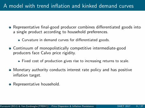
Intermediate-good firms

Minimize production costs s.t. technology

Yt(f ) =

{Nt(f )− φ if Nt(f ) ≥ φ0 otherwise.

Combining production function, intermediate-good demand, and labormarket clearing yields expression for output per hour

Yt

Nt=

(1− φ

Nt

)(st + ε

1 + ε

)−1

.

The RPD is a measure of demand dispersion:

st + ε

1 + ε=

∫ 1

0

Yt(f )

Ytdf .




Yt(f ) =



Yt

Nt=

(1− φ

Nt

)(st + ε

1 + ε

)−1

.


st + ε

1 + ε=

∫ 1

0

Yt(f )

Ytdf .




Yt(f ) =



Yt

Nt=

(1− φ

Nt

)(st + ε

1 + ε

)−1

.


st + ε

1 + ε=

∫ 1

0

Yt(f )

Ytdf .



Each period, a fraction α of firms keeps prices unchanged, while theremaining 1− α firms sets the price to maximize profits (p∗).

Under staggered price setting lags of price dispersion and RPD areendogenous state variables

(dt)1−θ(1+ε) = (1− α) (p∗t )1−θ(1+ε) + α

(dt−1

πt

)1−θ(1+ε)

(dt)−θ(1+ε) st = (1− α) (p∗t )−θ(1+ε) + α

(dt−1

πt

)−θ(1+ε)

st−1.



Each period, a fraction α of firms keeps prices unchanged, while theremaining 1− α firms sets the price to maximize profits (p∗).

Under staggered price setting lags of price dispersion and RPD areendogenous state variables

(dt)1−θ(1+ε) = (1− α) (p∗t )1−θ(1+ε) + α

(dt−1

πt

)1−θ(1+ε)

(dt)−θ(1+ε) st = (1− α) (p∗t )−θ(1+ε) + α

(dt−1

πt

)−θ(1+ε)

st−1.


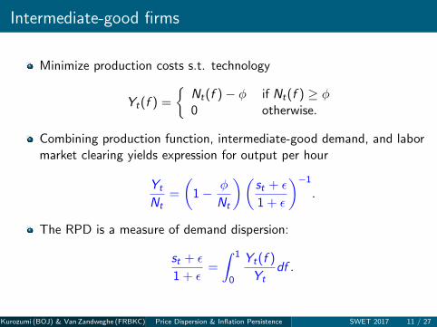
Monetary authority and household

Monetary authority sets the short-term interest rate according to aTaylor-type rule with interest rate smoothing:

log it = (1− ρ) [log i + φπ (logπt−logπ)] + ρ log it−1 + εt .

Representative household chooses final-good consumption, laborsupply, and riskless bonds to maximize utility

E0

∞∑t=0

βt

(logCt −

N1+σnt

1 + σn

)

subject to budget constraint.


Generalizing the NKPC

At the zero trend inflation rate or, equivalently, with full indexation tothe trend inflation rate,

πt = βEt πt+1 +(1− α)(1− αβ)

αmct .

At a positive trend inflation rate without price indexation, theNKPC generalizes as

πt = βEt πt+1 +(1− απθ−1)(1− αβπθ)

απθ−1mct + ϕt

where ϕt = αβπθEtϕt+1

+ β(π − 1)(1− απθ−1)[θEt πt+1 + (1− αβπθ)Etmct+1

].


Generalizing the NKPC

At the zero trend inflation rate or, equivalently, with full indexation tothe trend inflation rate,

πt = βEt πt+1 +(1− α)(1− αβ)

αmct .

At a positive trend inflation rate without price indexation, theNKPC generalizes as

πt = βEt πt+1 +(1− απθ−1)(1− αβπθ)

απθ−1mct + ϕt

where ϕt = αβπθEtϕt+1

+ β(π − 1)(1− απθ−1)[θEt πt+1 + (1− αβπθ)Etmct+1

].


Adding a kink in demand, inflation inherits inertia fromprice dispersion in generalized NKPC

πt = βEt πt+1 +(1− απγ−1)(1− αβπγ)

απγ−1[1− εγ/(γ − 1− ε)]mct + ϕt + ψt

− γ(1− απγ−1)[αβπγ−1(π − 1)(γ − 1) + ε(1− αβπγ)]

απγ−1[γ − 1− ε(γ + 1)]dt

+

(Et dt+1 −

1

απγ−1dt

)− αβπγ−1

(dt −

1

απγ−1dt−1

)using shorthand γ = θ(1 + ε) and ε = f (ε, α, β, θ, π).


Adding a kink in demand, inflation inherits inertia fromprice dispersion in generalized NKPC

πt = βEt πt+1 +(1− απγ−1)(1− αβπγ)

απγ−1[1− εγ/(γ − 1− ε)]mct + ϕt + ψt

− γ(1− απγ−1)[αβπγ−1(π − 1)(γ − 1) + ε(1− αβπγ)]

απγ−1[γ − 1− ε(γ + 1)]dt

+

(Et dt+1 −

1

απγ−1dt

)− αβπγ−1

(dt −

1

απγ−1dt−1

)using shorthand γ = θ(1 + ε) and ε = f (ε, α, β, θ, π).


Effects of RPD on the dynamics of inflation and outputper hour

RPD can increase inflation persistence through real marginal cost:

mct =

(1 +

σn

1 + φY

1+εs+ε

)Yt +

σns

s+ε

1 + φY

1+εs+ε

st .

RPD can change the sign of response of output per hour:

Yt − Nt =

(φ

Y

1 + ε

s + ε

)Nt −

s

s + εst . (1)


Quarterly calibration

Preferences and technology

β Subjective discount factor 0.99

σn Inverse of the elasticity of labor supply 0.5

α Probability of no price change 0.75

θ Parameter governing the price elasticity of demand 10

ε Degree of strategic complementarity −9, 0

Monetary policy

φπ Policy response to inflation 1.5

ρ Policy response to lag of interest rate 0.9

π Annualized trend inflation rate 2.5%


Impulse responses to a monetary policy shock in the caseof no kink in demand curves

0 5 10 15 20-0.6

-0.5

-0.4

-0.3

-0.2

-0.1

0

0.1

pp

Federal Funds Rate

0 5 10 15 20

0

0.2

0.4

0.6

0.8

1

pp


0 = 0;: = 2:5%

0 5 10 15 20


-0.2

0

0.2

0.4

0.6

0.8

1

1.2

%

Output

0 5 10 15 20


-0.1

-0.05

0

0.05

0.1

%

Output Per Hour


Trend inflation has minor influence on inflation persistencebut major influence on output per hour

0 5 10 15 20-0.6

-0.5

-0.4

-0.3

-0.2

-0.1

0

0.1

pp

Federal Funds Rate

0 5 10 15 20

0

0.2

0.4

0.6

0.8

1

pp


0 = 0;: = 2:5%0 = 0;: = 0

0 5 10 15 20


-0.2

0

0.2

0.4

0.6

0.8

1

1.2

%

Output

0 5 10 15 20


-0.1

-0.05

0

0.05

0.1

%

Output Per Hour


Kink gives rise to persistent and hump-shaped response ofinflation and positive response of output per hour

0 5 10 15 20-0.6

-0.5

-0.4

-0.3

-0.2

-0.1

0

0.1

pp

Federal Funds Rate

0 5 10 15 20

0

0.2

0.4

0.6

0.8

1

pp


0 = !9;: = 2:5%0 = 0;: = 2:5%0 = 0;: = 0

0 5 10 15 20


-0.2

0

0.2

0.4

0.6

0.8

1

1.2

%

Output

0 5 10 15 20


-0.1

-0.05

0

0.05

0.1

%

Output Per Hour


Persistent rise in price dispersion with muted response ofRPD

0 5 10 15 20


0

0.01

0.02

0.03

0.04

0.05

0.06

0.07

0.08

0.09

0.1

%

Relative Price Distortion (RPD)

0 = !90 = 0

0 5 10 15 20


0

0.05

0.1

0.15

0.2

0.25

%

Relative Price Dispersion


Effect of the kink in demand curves on the slope of the(generalized) NKPC

-9 -6 -3 0

0

0

0.02

0.04

0.06

0.08

0.1

Trend inflation rate = 2.5%Trend inflation rate = 0


Effects of a credible permanent decline in trend inflation

Volcker disinflation in early 1980s: gradual decline in inflation andrecession.

NKPC generates a gradual decline in inflation and a temporary declinein output, provided the model contains intrinsic inflation inertia.

Generalized NKPC generates similar responses, provided the modelcontains a kink in demand curves.


A one percentage point decline in trend inflation:NKPC with full price indexation to past inflation

0 5 10 15 20

Quarters since disinflation

-1

-0.9

-0.8

-0.7

-0.6

-0.5

-0.4

-0.3

-0.2

-0.1

0

pp d

evia

tion

from

initi

al s

tead

y st

ate

Inflation

0 = 0, indexation

0 5 10 15 20


-1.2

-1

-0.8

-0.6

-0.4

-0.2

0

0.2

0.4

% d

evia

tion

from

initi

al s

tead

y st

ate

Output


A one percentage point decline in trend inflation:Generalized NKPC but no kink in demand

0 5 10 15 20


-1

-0.9

-0.8

-0.7

-0.6

-0.5

-0.4

-0.3

-0.2

-0.1

0

pp d

evia

tion

from

initi

al s

tead

y st

ate

Inflation

0 = 00 = 0, indexation

0 5 10 15 20


-1.2

-1

-0.8

-0.6

-0.4

-0.2

0

0.2

0.4

% d

evia

tion

from

initi

al s

tead

y st

ate

Output


A one percentage point decline in trend inflation:Generalized NKPC and a kink in demand

0 5 10 15 20


-1

-0.9

-0.8

-0.7

-0.6

-0.5

-0.4

-0.3

-0.2

-0.1

0

pp d

evia

tion

from

initi

al s

tead

y st

ate

Inflation

0 = !90 = 00 = 0, indexation

0 5 10 15 20


-1.2

-1

-0.8

-0.6

-0.4

-0.2

0

0.2

0.4

% d

evia

tion

from

initi

al s

tead

y st

ate

Output


Conclusion

Models of the monetary transmission mechanism have difficultyaccounting for observed inflation inertia without assuming it isintrinsic.

A positive trend inflation rate has a minor influence on inflationpersistence and can induce a counterfactual response of productivityto a policy shock.

Combination of positive trend inflation, kink in demand curves, andfixed cost in production can generate responses of inflation andproductivity in line with empirical evidence.

Model improves responses to a transitory policy shock and apermanent disinflation.


Documents

Price Dispersion and Inflation Persistence