Price wars and collusion in the Spanish electricity market

23 (2005) 155–181

www.elsevier.com/locate/econbase

Price wars and collusion in the Spanish

electricity market

Natalia Fabraa,T, Juan Torob

aUniversidad Carlos III de Madrid, Spain, and CEPRbCentrA, Spain

Received 26 November 2002; received in revised form 15 January 2004; accepted 31 January 2005

Available online 7 April 2005

Abstract

We analyze the time-series of prices in the Spanish electricity market by means of a time varying–

transition-probability Markov-switching model. Accounting for changes in demand and cost

conditions (which reflect changes in input costs, capacity availability and hydro power), we show

that the time-series of prices is characterized by two significantly different price levels. Using a

Cournot model among contracted firms, we characterize firms’ optimal deviations from a collusive

agreement, and identify trigger variables that could be used to discourage deviations. By interpreting

the effects of the triggers in affecting the likelihood of starting a price war, we are able to infer some

of the properties of the collusive strategy that firms might have followed.

D 2005 Elsevier B.V. All rights reserved.

JEL classification: C22; L13; L94

Keywords: Electricity markets; Tacit collusion; Markov switching

1. Introduction

During the last decade decentralized electricity markets have been created in Britain,

Norway, Sweden, the United States, Australia, Argentina, and Spain, to name but a few.

0167-7187/$ -

doi:10.1016/j.

T Correspon

Getafe Madrid

E-mail add

International Journal of Industrial Organization

see front matter D 2005 Elsevier B.V. All rights reserved.

ijindorg.2005.01.004

ding author. Economics Department, Universidad Carlos III de Madrid, Calle Madrid 126, 28903

, Spain.

ress: [email protected] (N. Fabra).

N. Fabra, J. Toro / Int. J. Ind. Organ. 23 (2005) 155–181156

The details differ from country to country, but the different processes of reform share some

common features. These include the breaking up of the formerly vertically integrated

companies; the unbundling of generation, transmission, distribution and retailing; the

reliance on spot markets as a mean to allocate production and determine prices; and the

design of new institutional mechanisms to govern access to the transmission network.

This new form of regulation has raised concerns about the ability of electricity

producers to exercise market power and its effects on the efficiency of the market. The

recent empirical literature on market power in electricity markets is now vast. The studies

have identified strategic bidding and output decisions by individual firms (Borenstein and

Bushnell, 1999; Wolak, 2000, 2003; Wolfram, 1998) and have measured the departures of

market outcomes from the competitive benchmark (Borenstein et al., 2002; Joskow and

Kahn, 2002; Wolfram, 1999). All these studies have focused on the unilateral exercise of

market power, but little attention has been devoted to analyze collusive attempts to

exercise market power in a dynamic context.1 Nonetheless, electricity markets present

several features that facilitate the sustainability of collusion more than most other markets:

trading takes place on a daily basis and it is organized as a uniform-price auction,2 firms

are capacity constrained, demand is very inelastic in the short-term, and there is typically a

small number of players protected by high entry barriers. Both theory and experience

suggest that these factors may allow firms to coordinate their strategies, and hence

compete less aggressively with each other over time, through collusive agreements.

The analysis of the performance of the Spanish electricity spot market during 1998

provides a unique opportunity to perform an empirical analysis of firms’ dynamic

interaction. The availability of detailed data allows the use of changes in prices, firms’

market shares and cost fluctuations in order to identify potential attempts to exercise

market power in a dynamic context. Moreover, the analysis of this market uncovers

interesting effects regarding the link between firms’ bidding incentives and contract

positions. In the Spanish electricity market, firms are entitled to recover their stranded

costs through the so-called Competition Transition Costs (CTCs), which play a similar role

as contracts. In particular, given that CTCs are computed as a decreasing function of

market prices, they reduce firms’ incentives to raise prices. This effect is asymmetric

across firms, not only because firms’ market shares differ, but also because their (fixed)

shares over these payments are asymmetric. It is precisely this asymmetry that makes it

feasible to identify the effect of CTCs on firms’ bidding incentives.

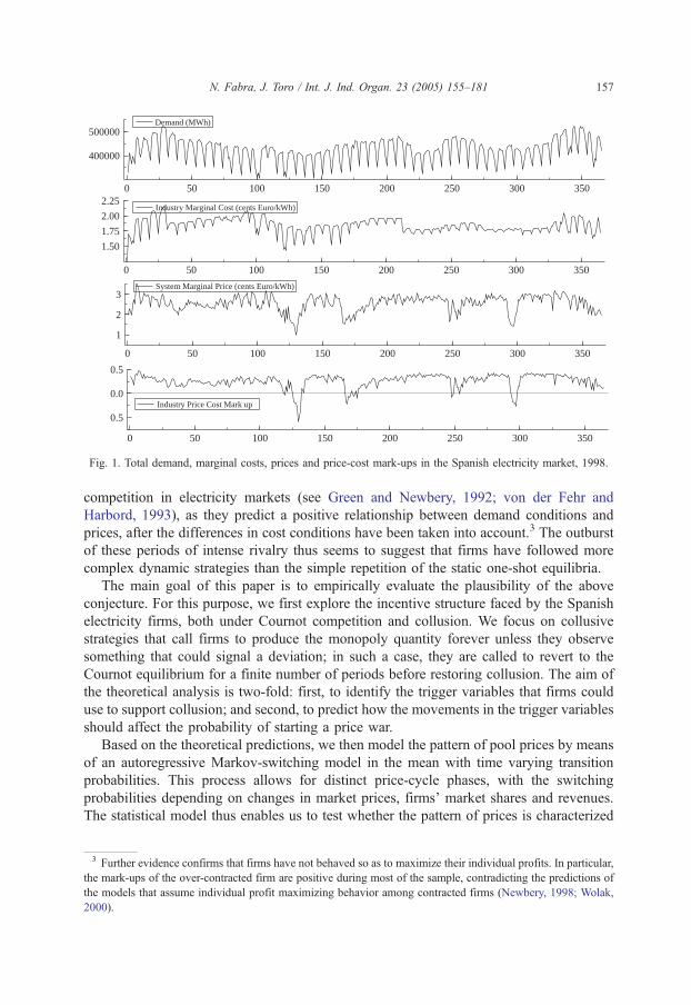
Fig. 1 plots the time series of demand, prices and the estimated marginal costs and

price-cost mark-ups in the Spanish electricity market from January 1998 to December

1998. Prices show a systematic relationship with the evolution of demand and cost

conditions throughout most of the time period. However, there are five to seven episodes

in which prices fall below their usual prevailing levels. These price jumps seem to be

uncorrelated with cost movements, as can be inferred from the series of price-cost mark-

ups. Furthermore, this pattern of prices is not consistent with the static models of price

1 Puller’s (2000) empirical analysis of collusion in the Californian electricity market is an exception.2 In a model applicable to electricity markets, Fabra (2003) shows that the sustainability of collusion is easier in

uniform-price auctions as compared to discriminatory auctions.

0 50 100 150 200 250 300 350

400000

500000Demand (MWh)

0 50 100 150 200 250 300 350

1.50

1.75

2.00

2.25Industry Marginal Cost (cents Euro/kWh)

0 50 100 150 200 250 300 350

1

2

3System Marginal Price (cents Euro/kWh)

0 50 100 150 200 250 300 350

0.5

0.0

0.5

Industry Price Cost Mark up

Fig. 1. Total demand, marginal costs, prices and price-cost mark-ups in the Spanish electricity market, 1998.

N. Fabra, J. Toro / Int. J. Ind. Organ. 23 (2005) 155–181 157

competition in electricity markets (see Green and Newbery, 1992; von der Fehr and

Harbord, 1993), as they predict a positive relationship between demand conditions and

prices, after the differences in cost conditions have been taken into account.3 The outburst

of these periods of intense rivalry thus seems to suggest that firms have followed more

complex dynamic strategies than the simple repetition of the static one-shot equilibria.

The main goal of this paper is to empirically evaluate the plausibility of the above

conjecture. For this purpose, we first explore the incentive structure faced by the Spanish

electricity firms, both under Cournot competition and collusion. We focus on collusive

strategies that call firms to produce the monopoly quantity forever unless they observe

something that could signal a deviation; in such a case, they are called to revert to the

Cournot equilibrium for a finite number of periods before restoring collusion. The aim of

the theoretical analysis is two-fold: first, to identify the trigger variables that firms could

use to support collusion; and second, to predict how the movements in the trigger variables

should affect the probability of starting a price war.

Based on the theoretical predictions, we then model the pattern of pool prices by means

of an autoregressive Markov-switching model in the mean with time varying transition

probabilities. This process allows for distinct price-cycle phases, with the switching

probabilities depending on changes in market prices, firms’ market shares and revenues.

The statistical model thus enables us to test whether the pattern of prices is characterized

3 Further evidence confirms that firms have not behaved so as to maximize their individual profits. In particular,

the mark-ups of the over-contracted firm are positive during most of the sample, contradicting the predictions of

the models that assume individual profit maximizing behavior among contracted firms (Newbery, 1998; Wolak,

2000).


by different price levels, whether the effects of the trigger variables are statistically

significant, and whether the signs of these effects coincide with those predicted by the

theory.

Our results support the hypothesis that two distinct price levels characterize the time

series of prices in the Spanish electricity market during 1998. Furthermore, most of the

triggers considered appear significant and they report the predicted signs. In particular, the

probability of starting a price war increases when the market share and revenues of the

over-contracted (under-contracted) firm increase (decrease) and the market price increases

above its usually prevailing level. In summary, our results suggest that the Spanish

electricity producers might have been alternating between episodes of collusion and price

wars, consistently with the theoretical predictions.

The paper is organized as follows. In the next section, we provide an overview of the

Spanish electricity industry and its market rules. In Section 3, we analyze a Cournot game

among contracted firms to understand firms’ incentive structure. Section 4 contains the

empirical analysis, including the data description, the empirical model, the summary of the

results, and their interpretation. Section 5 of the paper concludes.

2. The Spanish electricity industry

In 1997, the Spanish electricity industry experienced fundamental changes.4 It evolved

from a system in which the allocation of output among the electricity producers was based

on yardstick competition to one that relied on market forces as a way of finding the most

economic use of the available resources. Under the current regulatory design, transactions

are organized through a series of sequential markets—primarily, the day-ahead market and

the intra-day markets- and technical processes governed by the System Operator.

The day-ahead market concentrates most of the transactions.5 All available production

units, excluding those already committed to a physical contract, must participate in it as

suppliers. They are asked to submit, each day on a day-ahead basis, the minimum prices at

which they are willing to make their generation available in each of the 24 hourly

markets.6 The demand side is comprised of the distributors, retailers, external agents and

qualified consumers, who are also required to submit the maximum prices at which they

are willing to consume electricity, and commit in a similar fashion as suppliers. On the

basis of these supply and purchase bids, the Market Operator constructs the industry

supply and demand curves, ranking the production and demand units in increasing and

decreasing merit order, respectively. The intersection between the industry supply and

demand curves determines the market clearing price (the so-called System Marginal Price

4 The reforms were implemented through the Electricity Law 54/1997 of 27 November 1997. See Crampes and

Fabra (in press), Arocena et al. (1999) and Fabra Utray (2004) for an overview and discussion.

6 Sale and purchase bids can be made by considering from 1 to 25 energy blocks in each hour, with the

proposed price. The bid schedules have to be increasing (decreasing) in the quantity offered (demanded). The

supply bids can be simple, or they can include additional conditions, such as indivisibility, load gradient,

minimum income and scheduled shutdown.

5 In 1998, the daily market concentrated 99% of all the electricity traded.

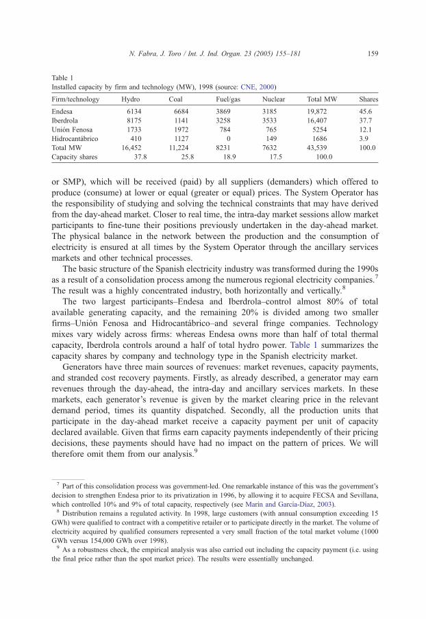
Table 1

Installed capacity by firm and technology (MW), 1998 (source: CNE, 2000)

Firm/technology Hydro Coal Fuel/gas Nuclear Total MW Shares

Endesa 6134 6684 3869 3185 19,872 45.6

Iberdrola 8175 1141 3258 3533 16,407 37.7

Union Fenosa 1733 1972 784 765 5254 12.1

Hidrocantabrico 410 1127 0 149 1686 3.9

Total MW 16,452 11,224 8231 7632 43,539 100.0

Capacity shares 37.8 25.8 18.9 17.5 100.0


or SMP), which will be received (paid) by all suppliers (demanders) which offered to

produce (consume) at lower or equal (greater or equal) prices. The System Operator has

the responsibility of studying and solving the technical constraints that may have derived

from the day-ahead market. Closer to real time, the intra-day market sessions allow market

participants to fine-tune their positions previously undertaken in the day-ahead market.

The physical balance in the network between the production and the consumption of

electricity is ensured at all times by the System Operator through the ancillary services

markets and other technical processes.

The basic structure of the Spanish electricity industry was transformed during the 1990s

as a result of a consolidation process among the numerous regional electricity companies.7

The result was a highly concentrated industry, both horizontally and vertically.8

The two largest participants–Endesa and Iberdrola–control almost 80% of total

available generating capacity, and the remaining 20% is divided among two smaller

firms–Union Fenosa and Hidrocantabrico–and several fringe companies. Technology

mixes vary widely across firms: whereas Endesa owns more than half of total thermal

capacity, Iberdrola controls around a half of total hydro power. Table 1 summarizes the

capacity shares by company and technology type in the Spanish electricity market.

Generators have three main sources of revenues: market revenues, capacity payments,

and stranded cost recovery payments. Firstly, as already described, a generator may earn

revenues through the day-ahead, the intra-day and ancillary services markets. In these

markets, each generator’s revenue is given by the market clearing price in the relevant

demand period, times its quantity dispatched. Secondly, all the production units that

participate in the day-ahead market receive a capacity payment per unit of capacity

declared available. Given that firms earn capacity payments independently of their pricing

decisions, these payments should have had no impact on the pattern of prices. We will

therefore omit them from our analysis.9

7 Part of this consolidation process was government-led. One remarkable instance of this was the government’s

decision to strengthen Endesa prior to its privatization in 1996, by allowing it to acquire FECSA and Sevillana,

which controlled 10% and 9% of total capacity, respectively (see Marın and Garcıa-Dıaz, 2003).

9 As a robustness check, the empirical analysis was also carried out including the capacity payment (i.e. using

the final price rather than the spot market price). The results were essentially unchanged.

8 Distribution remains a regulated activity. In 1998, large customers (with annual consumption exceeding 15

GWh) were qualified to contract with a competitive retailer or to participate directly in the market. The volume of

electricity acquired by qualified consumers represented a very small fraction of the total market volume (1000

GWh versus 154,000 GWh over 1998).


Last, the incumbent generators are entitled to recover their stranded costs through the so-

called Competition Transition Costs (CTC) during a 10-year period. The maximum amount

of these payments was computed as the difference between the net present value of the

revenues that firms were entitled to receive under the former regulatory regime and firms’

market expected revenues, under the assumption that the competitive market price would be

3.6 c/kWh on average. The amount of CTCs to be paid to the whole industry in a particular

year is computed as the difference between the total revenues earned through the regulated

tariff and the regulated costs.10 The Law 54/1997 established that this residual amount

would be shared among firms on the basis of some predetermined shares: 51.2% for

Endesa, 27.1% for Iberdrola, 12.9% for Union Fenosa and 5.7% for Hidrocantabrico.

Two conditions were imposed on the value of the CTCs to be received by a firm over

the transition period. First, if the average price received by a firm exceeded 3.6 c/kWh, the

extra revenues should be deducted from the firm’s maximum CTC entitlement. And

second, a firm’s CTC revenues could not exceed the maximum entitlement established by

the Law 54/1997. These two conditions imposed a price-cap and a price-floor on the pool

price. On the one hand, it would not be profitable for any firm to raise prices over 3.6 c/

kWh, as any increase in market revenues would be offset by the reduction in the firm’s

total CTC entitlement.11 On the other hand, it would not be profitable to reduce prices to a

level below one that allowed a firm to obtain its maximum entitlement, given that the

reduced market revenues would not be compensated by an increase in its CTC revenues.12

In the next section we present and solve a simple game that incorporates some of the

features of the Spanish electricity market that are relevant in understanding firms’ pricing

incentives.

3. The theoretical framework

Consider an industry in which two firms simultaneously decide how much to produce,

qi, i=1, 2, at constant marginal costs cz0. The market price is determined as a function of

firms’ quantity choices, P( q1+q2), where P (d ) is the inverse demand function, which is

decreasing in the total quantity produced. Furthermore, we assume that firm i=1, 2 is

entitled to receive an extra-payment [s�P( qi+qj)]ai, where s is a fixed tariff and ai is

firm i’s (exogenously given) contracted quantity. Firms’ contract positions are taken as a

proxy for CTCs. We will assume P(a1+a2)Nc.

10 Mainly, payments to distributors (who are reimbursed their costs of buying electricity in the spot market plus a

rate of return), payments for transmission, payments to generators in the so-called Special Regime (mainly,

renewables and cogenerators) and subsidies for burning national coal.11 This assertion is valid as long as firms do not discount the future stream of profits very strongly, and as long as

they perceive full regulatory certainty about the payment of their total CTC entitlements. This second concern

started to play a role from 1999 onwards, when the European Commission opened up an investigation to

determine whether the CTCs were State Aids, in which case they would have been banned.12 The maximum amount of CTCs was fixed at 11,951.5m, 1774.6 of which were subsidies to national coal, and

the rest was the maximum amount to be divided among the incumbent firms. In 1998, firms perceived CTCs

which amounted to 633.5m. The maximum entitlements of Endesa and Iberdrola were reduced by o67.5m and

o47.15m, respectively, because their average prices exceeded 3.6 co/kW h. See CNE (2000) for a more detailed

description.


First, assume that firms choose their quantities non-cooperatively. Firm i’s profit

maximization problem given an output level qj of the rival firm, i=1, 2, ip j, is:13

maxqiz0

pi qi; qj� �

¼ P qi þ qj� �

� c� �

qi þ s � P qi þ qj� ��

ai

An optimal quantity choice for firm i given its rival’s output must therefore satisfy the

first-order condition:

P V qi þ qj� �

qi � ai½ � þ P qi þ qj� �

� c ¼ 0 ð1Þ

For each qj, we let Ri( qj) denote firm i’s best response function. A pair of quantity choices

( q1*,q2*) is a Nash equilibrium if and only if these quantities satisfy the first-order condition

(1) for the two firms.

Second, assume that firms choose quantities so as maximize joint profits. Their

maximization problem is given by:14

maxqz0

pm qð Þ ¼ P qð Þ � c½ �qþ s � P qð Þ½ � a1 þ a2½ �

The monopoly quantity, denoted qm, must satisfy the first-order condition:

P V qmð Þ qm � a1 þ a2ð Þ½ � þ P qmð Þ � c ¼ 0 ð2Þ

Therefore, any quantity profile ( q1m,q2

m) such that q1m+q2

m=qm would allow firms to

attain monopoly profits. However, as shown in Proposition 1 below, unless each firm’s

production at the monopoly solution equals its contracted quantity, i.e., qim=ai, i=1, 2,

firms will have unilateral incentives to deviate. Proposition 1 further explores the

conditions under which a firm will optimally deviate from the monopoly solution by either

reducing or increasing output.

Proposition 1. From any quantity profile (q1m,q2

m) such that q1m+q2

m=qm, firm i’s optimal

deviation is to reduce output if and only if the rival is over-contracted at the monopoly

solution. Formally, Ri (qjm)bqi

mfqjmbaj.

Proof.We proceed by comparing the marginal profit functions (1) and (2). Graphically, we

want to assess whether the slope of the tangent to a firm’s individual profit function

evaluated at the monopoly quantities is upward or downward sloping.

Extracting (2) from (1) evaluated at ( qim,qj

m), for i=1, 2, ip j, we obtain

Bpi qmi ; qmj

� �Bqi

�Bpm qmi þ qmj

� �Bqi

¼ � P V qmð Þ � qmj � ajh i

:

Given that the first-order condition for the monopolist is satisfied with equality,

and given that PV( q)b0, it follows that firm i’s marginal profit function is downward

13 We assume that the objective function is concave in qi so that satisfaction of first order condition is sufficient

for Ri( qj) to be firm i’s optimal choice given the production of its rival.14 Again, we assume that the objective function is concave in q so that satisfaction of first order condition is

sufficient for qm to be an optimal choice.


sloping at ( qim,qj

m) if and only if the rival firm is over-contracted at the monopoly

solution, i.e.,

Bpi qmi ; qmj

� �Bqi

b0fqmj baj:

From the concavity of the profit function, it follows that a firm facing an over-

contracted rival deviates from the monopoly solution by reducing output. Note that in a

standard game with no contract positions, qjmNaj=0. Hence, in the absence of contracts,

we obtain the standard result that a firm’s best response is always to increase output.

5

To illustrate our previous results, suppose that the demand function takes the linear

form P( q)=1�q1�q2. Assumption P(a1+a2)Nc implies 1�a1�a2N0.Using (2), the monopoly outcome is characterized by

qm ¼ 1þ a1 þ a22

P qmð Þ ¼ 1� a1 � a22

pm ¼ 1� a1 � a22

2þ s a1 þ a2½ �

Similarly, using the first-order condition (1), we find that firm i’s reaction function is15

Ri qj� �

: qi ¼1� qj

2þ ai

2; i ¼ 1; 2; ipj: ð3Þ

Solving the system of reaction functions, the Cournot equilibrium outcome is

characterized, for i=1,2, by

q4i ¼1� aj þ 2ai

3

P q4i ; q4j

� �¼ 1� a1 � a2

3

pi q4i ; q4j

� �¼ 1� ai � aj

3

2þ sai:

By comparing the monopoly and the Cournot solutions, note that the monopoly price

exceeds the Cournot price. Nevertheless, whenever firms’ contracted quantities are

sufficiently large, i.e., a1+a2N1/3 , collusion among contracted firms yields lower prices

15 Note that a firm’s contracted quantity shifts its reaction function out, but does not affect its slope.


than Cournot competition among non-contracted firms. That is, contracts make colluding

firms more aggressive, even absent price wars.

To analyze whether a deviant firm increases or decreases its production with respect to

the monopoly solution, we extract qim from the reaction function (3) evaluated at qj

m:

Ri qmj

� �� qmi ¼

qmj � aj2

Hence, as stated in Proposition 1 above, the optimal deviation involves reducing output

if the rival firm is over-contracted.

Last, we are interested in identifying the observable consequences of firms’ optimal

deviations. Building on Proposition 1, if a firm facing an over-contracted rival deviates, it

would do so by reducing its output. Such a deviation would cause a reduction in its market

share, an increase in prices, and accordingly, an increase in its rival’s market revenues.

Similarly, if a firm facing an under-contracted rival deviates, it would do so by increasing

output. Such a deviation would cause an increase in its market share, a reduction in prices,

and accordingly, a reduction in its rival’s market revenues.

The following corollary summarizes these effects.

Corollary 1. Index firms such that firm 1 is over-contracted and firm 2 is undercontracted,

i.e., q1mba1 and q2

mNa2:

(i) An optimal deviation by either firm would cause a reduction (increase) in firm 2’s

(firm 1’s) market share. If q1mNq2

m; it would also lead to an increase in the

Herfindahl–Hirschman Index (i.e., the sum of the squared market shares).

(ii) An optimal deviation by firm 1 would reduce prices and firm 2’s market revenues.

An optimal deviation by firm 2 would increase prices and firm 1’s market revenues.

3.1. Empirical predictions

The Cournot model developed above allows us to derive some empirical

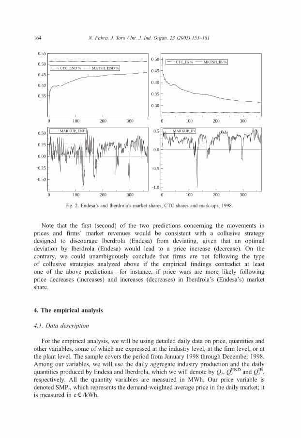
predictions. From Fig. 2, note that Endesa is over-contracted, that Iberdrola is

under-contracted, and that Endesa’s production exceeds Iberdrola’s during most of the

sample. Hence, applying Corollary 1, the empirical findings listed below would be

consistent with firms following some sort of collusive strategy that calls firms to compete

fiercely with each other only after observing something that could signal a deviation (in

the right direction).

Changes in firms’ market shares: The probability of starting a price war increases

following a reduction in Iberdrola’s market share and an increase in Endesa’s market share.

Equivalently, price wars are more likely following an increase in the HHI.

Changes in prices and firms’ market revenues: If a price increase makes a price war

more likely, an increase in Endesa’s market revenues should also increase the probability

of starting a price war. Alternatively, if a price reduction makes a price war more likely, a

reduction in Iberdrola’s market revenues should also increase the probability of starting a

price war.

0 100 200 300

0.35

0.40

0.45

0.50

0.55

CTC_END % MKTSH_END %

0 100 200 300

0.30

0.35

0.40

0.45

0.50CTC_IB % MKTSH_IB %

0 100 200 300

-0.50

-0.25

0.00

0.25

0.50 MARKUP_END

0 100 200 300

-1.0

-0.5

0.0

0.5 MARKUP_IB

Fig. 2. Endesa’s and Iberdrola’s market shares, CTC shares and mark-ups, 1998.


Note that the first (second) of the two predictions concerning the movements in

prices and firms’ market revenues would be consistent with a collusive strategy

designed to discourage Iberdrola (Endesa) from deviating, given that an optimal

deviation by Iberdrola (Endesa) would lead to a price increase (decrease). On the

contrary, we could unambiguously conclude that firms are not following the type

of collusive strategies analyzed above if the empirical findings contradict at least

one of the above predictions—for instance, if price wars are more likely following

price decreases (increases) and increases (decreases) in Iberdrola’s (Endesa’s) market

share.

4. The empirical analysis

4.1. Data description

For the empirical analysis, we will be using detailed daily data on price, quantities and

other variables, some of which are expressed at the industry level, at the firm level, or at

the plant level. The sample covers the period from January 1998 through December 1998.

Among our variables, we will use the daily aggregate industry production and the daily

quantities produced by Endesa and Iberdrola, which we will denote by Qt, QtEND and Qt

IB,

respectively. All the quantity variables are measured in MWh. Our price variable is

denoted SMPt, which represents the demand-weighted average price in the daily market; it

is measured in co/kWh.


In addition, we have constructed estimates of marginal costs and mark-ups (Borenstein

et al., 2002; Joskow and Kahn, 2002; Wolfram, 1999 use similar estimation techniques).

For this purpose, we have first derived the shot-run thermal cost curve at the firm level by

estimating the marginal production costs for each generating plant, on a daily basis.16 The

short-run marginal costs of a thermal plant (including nuclear, coal, oil and natural gas

plants) depend on the type of fuel it burns, the cost of the fuel, the plant’s heat rate (i.e., the

efficiency rate at which each plant converts the heat content of the fuel into output), and

the short-run variable cost of operating and maintaining the plant (O&M).17 We have

assumed that the costs of the fossil-fuels are those negotiated daily in the international

input markets.18 In addition, to calculate the cost of the coal plants, we have added an

estimate of transportation costs based on the distance between each plant and the nearest

harbor where coal is delivered. Last, we have assumed that the available capacity of each

plant equals its average availability over a given month in those days in which the plant

was not subject to scheduled maintenance or forced outages; a plant’s available capacity is

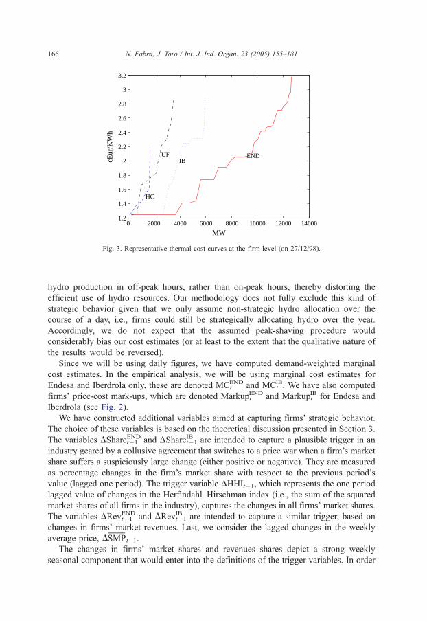
assumed to be zero otherwise.19 By aggregating the capacities of a firm’s thermal plants in

increasing cost order, we obtain an estimate of its thermal cost curve in a given day (see

Fig. 3).

To obtain hourly marginal cost estimates, we need to intersect each firm’s thermal

cost curve with its thermal production in every hour, i.e., its total production net of its

hydro production. For this purpose, we need to assume how firms allocate total hydro

production during the day, given that we lack information on the hourly figures. Our

data set distinguishes between each firm’s daily pondage hydro and run of the river.

Whereas firms can choose when to allocate the former, they cannot choose when to

produce with the latter. Hence, we have allocated run of the river production evenly over

the day. For pondage hydro, we have assumed that firms use it non-strategically and

allocate it to high demand hours. This results in firms equalizing thermal production

across the hours in which they allocate pondage hydro power, i.e., firms peak-shave

each hour. Bushnell (2003) finds that strategic firms may have an incentive to increase

16 There are intertemporal and operational constraints that affect firms’ costs (e.g. start-up costs or ramping

rates). Our cost estimation does not take these into account (see Borenstein et al., 2002 for a discussion of how

this could affect the estimates).17 The information on the types of fuel burned by each plant, together with their heat rates and operating and

maintenance costs, has been obtained from Red Electrica de Espana (REE is the Spanish Transmission Owner and

System Operator).18 We have not considered firms’ obligation to burn domestic coal, and the subsidies obtained from so doing. For

coal units, we use the MCIS Index, for fuel units we use the F.O. 1% CIF NWE prices, and for gas units we use

the Gazexport–Ruhrgas prices. All series are in co/te. We have obtained this information from UNESA (the

Spanish National Union of Electricity companies). For nuclear plants, we have assumed a fixed input cost equal to

0.5 co/te; this does not affect the results as nuclear plants are never marginal.19 In a study of the British electricity market, Wolfram (1999) assigns each plant a capacity below its declared

capacity to capture the strategic withholding aimed at increasing capacity payments (Patrick and Wolak, 1997). In

the Spanish electricity market, capacity payments are fixed per MW declared available, implying that firms do not

have incentives to under-declare their available capacities. Nevertheless, it must be noted that the scheduling of

planned outages for maintenance may be subject to strategic considerations (e.g. it may be profitable to shift

scheduled outages from off-peak to on-peak periods, see Patrick and Wolak, 1997 for evidence on this).

0 2000 4000 6000 8000 10000 12000 140001.2

1.4

1.6

1.8

2

2.2

2.4

2.6

2.8

3

3.2

END IB

UF

HC

MW

cEur

/KW

h

Fig. 3. Representative thermal cost curves at the firm level (on 27/12/98).


hydro production in off-peak hours, rather than on-peak hours, thereby distorting the

efficient use of hydro resources. Our methodology does not fully exclude this kind of

strategic behavior given that we only assume non-strategic hydro allocation over the

course of a day, i.e., firms could still be strategically allocating hydro over the year.

Accordingly, we do not expect that the assumed peak-shaving procedure would

considerably bias our cost estimates (or at least to the extent that the qualitative nature of

the results would be reversed).

Since we will be using daily figures, we have computed demand-weighted marginal

cost estimates. In the empirical analysis, we will be using marginal cost estimates for

Endesa and Iberdrola only, these are denoted MCtEND and MCt

IB. We have also computed

firms’ price-cost mark-ups, which are denoted MarkuptEND and Markupt

IB for Endesa and

Iberdrola (see Fig. 2).

We have constructed additional variables aimed at capturing firms’ strategic behavior.

The choice of these variables is based on the theoretical discussion presented in Section 3.

The variables DShareENDt�1 and DShareIBt�1 are intended to capture a plausible trigger in an

industry geared by a collusive agreement that switches to a price war when a firm’s market

share suffers a suspiciously large change (either positive or negative). They are measured

as percentage changes in the firm’s market share with respect to the previous period’s

value (lagged one period). The trigger variable DHHIt�1, which represents the one period

lagged value of changes in the Herfindahl–Hirschman index (i.e., the sum of the squared

market shares of all firms in the industry), captures the changes in all firms’ market shares.

The variables DRevENDt�1 and DRevIBt�1 are intended to capture a similar trigger, based on

changes in firms’ market revenues. Last, we consider the lagged changes in the weekly

average price, DSMPt�1.

The changes in firms’ market shares and revenues shares depict a strong weekly

seasonal component that would enter into the definitions of the trigger variables. In order

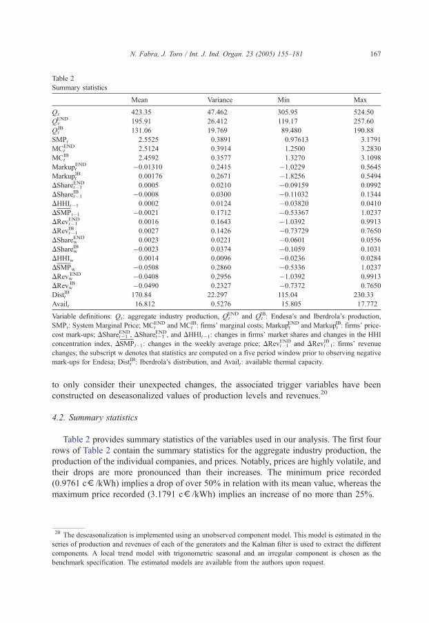
Table 2

Summary statistics

Mean Variance Min Max

Qt 423.35 47.462 305.95 524.50

QtEND 195.91 26.412 119.17 257.60

QtIB 131.06 19.769 89.480 190.88

SMPt 2.5525 0.3891 0.97613 3.1791

MCtEND 2.5124 0.3914 1.2500 3.2830

MCtIB 2.4592 0.3577 1.3270 3.1098

MarkuptEND �0.01310 0.2415 �1.0229 0.5645

MarkuptIB 0.00176 0.2671 �1.8256 0.5494

DShareENDt�1 0.0005 0.0210 �0.09159 0.0992

DShareIBt�1 �0.0008 0.0300 �0.11032 0.1344

DHHIt�1 0.0002 0.0124 �0.03820 0.0410

DSMP t�1 �0.0021 0.1712 �0.53367 1.0237

DRevENDt�1 0.0016 0.1643 �1.0392 0.9913

DRevIBt�1 0.0027 0.1426 �0.73729 0.7650

DShareENDw 0.0023 0.0221 �0.0601 0.0556

DShareIBw �0.0023 0.0374 �0.1059 0.1031

DHHIw 0.0014 0.0096 �0.0236 0.0284

DSMPw �0.0508 0.2860 �0.5336 1.0237

DRevwEND �0.0408 0.2956 �1.0392 0.9913

DRevwIB �0.0490 0.2327 �0.7372 0.7650

DisttIB 170.84 22.297 115.04 230.33

Availt 16.812 0.5276 15.805 17.772

Variable definitions: Qt: aggregate industry production, QtEND and Qt

IB: Endesa’s and Iberdrola’s production,

SMPt: System Marginal Price; MCtEND and MCt

IB: firms’ marginal costs; MarkuptEND and Markupt

IB: firms’ price-

cost mark-ups; DShareENDt�1 , DShareENDt�1 , and DHHIt�1: changes in firms’ market shares and changes in the HHI

concentration index, DSMP t�1: changes in the weekly average price; DRevENDt�1 and DRevIBt�1: firms’ revenue

changes; the subscript w denotes that statistics are computed on a five period window prior to observing negative

mark-ups for Endesa; DisttIB: Iberdrola’s distribution, and Availt: available thermal capacity.


to only consider their unexpected changes, the associated trigger variables have been

constructed on deseasonalized values of production levels and revenues.20

4.2. Summary statistics

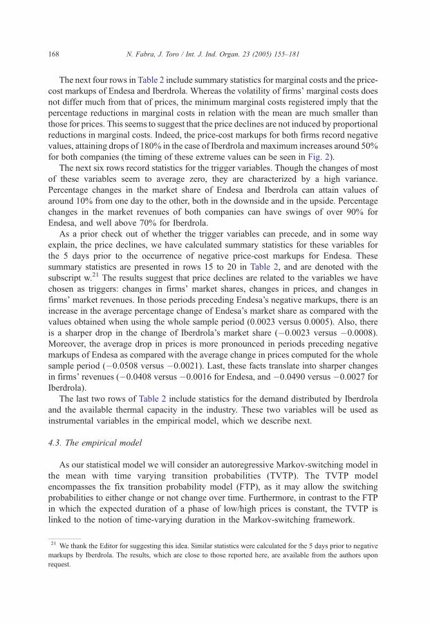
Table 2 provides summary statistics of the variables used in our analysis. The first four

rows of Table 2 contain the summary statistics for the aggregate industry production, the

production of the individual companies, and prices. Notably, prices are highly volatile, and

their drops are more pronounced than their increases. The minimum price recorded

(0.9761 co/kWh) implies a drop of over 50% in relation with its mean value, whereas the

maximum price recorded (3.1791 co/kWh) implies an increase of no more than 25%.

20 The deseasonalization is implemented using an unobserved component model. This model is estimated in the

series of production and revenues of each of the generators and the Kalman filter is used to extract the different

components. A local trend model with trigonometric seasonal and an irregular component is chosen as the

benchmark specification. The estimated models are available from the authors upon request.


The next four rows in Table 2 include summary statistics for marginal costs and the price-

cost markups of Endesa and Iberdrola. Whereas the volatility of firms’ marginal costs does

not differ much from that of prices, the minimum marginal costs registered imply that the

percentage reductions in marginal costs in relation with the mean are much smaller than

those for prices. This seems to suggest that the price declines are not induced by proportional

reductions in marginal costs. Indeed, the price-cost markups for both firms record negative

values, attaining drops of 180% in the case of Iberdrola andmaximum increases around 50%

for both companies (the timing of these extreme values can be seen in Fig. 2).

The next six rows record statistics for the trigger variables. Though the changes of most

of these variables seem to average zero, they are characterized by a high variance.

Percentage changes in the market share of Endesa and Iberdrola can attain values of

around 10% from one day to the other, both in the downside and in the upside. Percentage

changes in the market revenues of both companies can have swings of over 90% for

Endesa, and well above 70% for Iberdrola.

As a prior check out of whether the trigger variables can precede, and in some way

explain, the price declines, we have calculated summary statistics for these variables for

the 5 days prior to the occurrence of negative price-cost markups for Endesa. These

summary statistics are presented in rows 15 to 20 in Table 2, and are denoted with the

subscript w.21 The results suggest that price declines are related to the variables we have

chosen as triggers: changes in firms’ market shares, changes in prices, and changes in

firms’ market revenues. In those periods preceding Endesa’s negative markups, there is an

increase in the average percentage change of Endesa’s market share as compared with the

values obtained when using the whole sample period (0.0023 versus 0.0005). Also, there

is a sharper drop in the change of Iberdrola’s market share (�0.0023 versus �0.0008).

Moreover, the average drop in prices is more pronounced in periods preceding negative

markups of Endesa as compared with the average change in prices computed for the whole

sample period (�0.0508 versus �0.0021). Last, these facts translate into sharper changes

in firms’ revenues (�0.0408 versus �0.0016 for Endesa, and �0.0490 versus �0.0027 for

Iberdrola).

The last two rows of Table 2 include statistics for the demand distributed by Iberdrola

and the available thermal capacity in the industry. These two variables will be used as

instrumental variables in the empirical model, which we describe next.

4.3. The empirical model

As our statistical model we will consider an autoregressive Markov-switching model in

the mean with time varying transition probabilities (TVTP). The TVTP model

encompasses the fix transition probability model (FTP), as it may allow the switching

probabilities to either change or not change over time. Furthermore, in contrast to the FTP

in which the expected duration of a phase of low/high prices is constant, the TVTP is

linked to the notion of time-varying duration in the Markov-switching framework.

21 We thank the Editor for suggesting this idea. Similar statistics were calculated for the 5 days prior to negative

markups by Iberdrola. The results, which are close to those reported here, are available from the authors upon

request.


The autoregressive TVTP Markov-switching model of prices allows for distinct price-

cycle phases (collusive price phase/price war phase) with state-dependent means, and for

dynamics of prices with the lagged predetermined variables.22 The state of prices is not

known with certainty. The econometrician can neither observe the state of prices nor

deduce the state directly. These states are assumed to be path dependent and evolve

according to a first-order Markov process with TVTP coefficients. The TVTP model with

state-dependent mean can be presented as:23

SMPt ¼ lStþ bZt þ vst

lSt¼ l0 1� Stð Þ þ l1St

St ¼ 0; 1: ð4Þ

where SMPt is the system marginal price in period t; lStis the mean of prices in state St;

which can either be a collusive state, St=0, or a price war state, St=1 (i.e., l0zl1), and Zt

is a group of variables that are likely to influence prices and measured as deviations from

their means.

The stochastic process for St can be summarized by the following transition probability:

P St ¼ stjSt�1 ¼ st�1;wt�1ð Þ;

where st is a possible realization of the random variable St. We assume serial correlation of

the states (e.g. a collusive period is likely to be followed by another collusive period). The

variable wt�1 is likely to influence the transition probabilities, and it is henceforth referred

to as dtrigger variableT.24,25

The matrix of transition probabilities that governs the stochastic process is given by:

Kt�1 ¼q wt�1ð Þ 1� p wt�1ð Þ1� q wt�1ð Þ p wt�1ð Þ

�;

�ð5Þ

22 In this respect, we depart from Ellison (1994) since he allows for autoregressive residuals, which in our view

could be a sign of misspecification because of the omission of lagged dependent variables.

24 Two issues need to be stressed. First, we have explicitly written lagged wt�1, because the theory predicts that

firms should react immediately after they observe an anomalous behavior of the trigger variables. And second, it

might be reasonable to allow the transition probability p(wt�1) to depend on the number of periods firms have

been in a price war, i.e. on duration, dt�1. We are aware that omitting the dependence of p(wt�1) on dt�1 might

lead to inconsistent estimates of the response of wt�1 on p. This should not affect our main results however. We

are only interested in determining the probability of entering into a price war, 1�q(wt�1); which should not be

dependent on duration.25 In order to obtain consistent and normally distributed estimates from our maximum likelihood estimators, the

trigger-variables chosen should be conditionally uncorrelated with the states, given the current prices (see Engle et

al., 1983; Filardo, 1994). This would allow us to estimate consistently our TVTP model using jointly the

conditional maximum likelihood estimator (MLE) and the filtering methods proposed in Hamilton (1989). This is

the case of our trigger variables.

23 Eq. (4) could include the trigger-variables (wt�1). However, we formulate our model with the trigger-variables

influencing only the transition probabilities, to emphasize the contribution of the TVTP on the price dynamics.


where q(wt�1)=P(St=0|St�1=0; wt�1) and p(wt�1)=P(St=0|St�1=1; wt�1). In words,

q(wt�1) captures the probability of being in a collusive state (St=0) given that the previous

period was a collusive state (St�1=0) and given the values recorded for the trigger variable

in the previous period (wt�1). That is, the probability of switching to a given state

(collusion/price war) depends on the given state and the value of the trigger variable in the

previous period.

In searching for a particular functional form of the transition probabilities, we will use

the logistic function:26

P St ¼ kjSt�1 ¼ l;wt�1ð Þ ¼exp klk;0 þ klk;1wt�1

� �1þ exp klk;0 þ klk;1wt�1

� � ; l; k ¼ 0; 1:

where (klk, l, k=0, 1) are unrestricted parameters. We are interested in characterizing the

probability of starting a price war. This is given by

1� q wt�1ð Þ ¼ P St ¼ 1jSt�1 ¼ 0;wt�1ð Þ ¼ 1�exp k00;0 þ k00;1wt�1

� �1þ exp k00;0 þ k00;1wt�1

� � : ð6Þ

Thus the parameter estimate k00,1 reflects the influence of wt�1 on 1�q(wt�1).27

With autoregressive dynamics of order 1 the conditional density distribution of SMPt,

given St, St�1, SMPt�1, wt�1 and Zt, is defined by f, and can be written as:

f SMPtjSt; St�1; SMPt�1;wt�1;Ztð Þ

¼X1st¼0

X1st�1¼0

f SMPt; St ¼ st; St�1 ¼ st�1jSMPt�1;wt�1;Ztð Þ

¼X1st¼0

X1st�1¼0

f SMPtjSt ¼ st; St�1 ¼ st�1; SMPt�1;wt�1;Ztð Þ

P St ¼ st; St�1 ¼ st�1jSMPt�1;wt�1;Ztð Þ

¼X1st¼0

X1st�1¼0

f SMPtjSt ¼ st; St�1 ¼ st�1; SMPt�1;wt�1;Ztð Þ

P St ¼ stjSt�1 ¼ st�1;wt�1ð ÞP St�1 ¼ st�1jwt�1ð Þ

26 As in binary response models different specifications are available for mapping the index function

(k lk ,0+k lk ,1wt�1, k, l=0, 1) into a probability. We could have tried other alternatives for our transformation

function ( F(d )) such as a normal or a Cauchy cumulative distribution function instead of the logistic specification

chosen. However, we have preferred the latter specification since it is more tractable. For the normal and Cauchy

cumulative distribution function there is no close form expression for F(x) and it has to be evaluated numerically.

This would have increased the amount of calculations in the type of models that we use in the paper which are

already very computer intensive.27 Note that the sign of marginal effect of wt�1 on the probability of starting a price war will have the opposite

sign as the E00,1s.


and the likelihood function is:

L hð Þ ¼XTt¼1

ln f SMPtjSMPt�1;Zt;wt�1; hð Þ;

where h are the parameters of interest. The states are unobserved by the econometrician

and the filter developed in Hamilton (1989) is used to jointly estimate the parameters of

the model and the process governing the states.

In order to analyze the pattern of prices in the Spanish electricity market, we will

estimate a supply equation of the form,

SMPt ¼ b0 þ b1MCENDt þ b2MCIB

t þ b3QENDt þ b4Q

IBt þ b5Q

Rt : ð7Þ

Our supply equation defines SMPt as function of a constant, b0, the marginal cost of the

main generators, MCtEND and MCt

IB; their production levels, QtEND and Qt

IB, and the

residual demand not served by them, QtR=[Qt�Qt

END�QtIB] (i.e., covered through

imports, the production of the non-strategic firms, etc.).

Our previous discussion suggests that in the Spanish electricity market the SMPt might

be better characterized by a changing mean, with two different price levels, and that the

dynamics of switching from one price state to the other might be influenced by some

strategic variables. In order to formulate Eq. (7) as in (4), we express the variables in

deviations from their means and allow the mean of prices to fluctuate between two states.

Last, we introduce autoregressive dynamics to allow for cross-price effects. This results in

our equation of interest,

SMPt � lSt¼ q SMPt�1 � lSt�1

� �þ bZt þ vst ð8Þ

where b is the vector of parameters in the linear part of the model, Zt=[MCtEND�

E(MCtEND), MCt

IB�E(MCtIB), Qt

END�E(QtEND), Qt

IB�E(QtIB), Qt

R�E(QtR)]V is the

corresponding vector of variables measured in deviations from their means, the

term vts~N(0,rs) captures innovations or shocks unmodelled in our supply equation

and lStdenotes the time varying mean of prices, where St denotes the state, with St=0

if t is a collusive period (high prices), and St=1 if t belongs to a price war (low

prices).

Note that there could be three potential sources of endogeneity of the Zt variables. The

demand not served by the strategic firms, QtR, and the quantities they produce, Qt

END and

QtIB, are likely to be correlated with innovations in our price Eq. (8). In order to address

this endogeneity problem we respectively instrument these variables with weekend

dummies, the available thermal capacity in the industry, and the demand distributed by

Iberdrola (see Table 2 for summary statistics of these variables). These are all valid

instruments as they are correlated with the corresponding variables but unrelated with

innovations in prices. The weekend dummies capture most of the variation of the demand

not served by the strategic firms and they are unrelated with innovations in prices.

Moreover, the thermal available capacity should be correlated with QtEND and uncorrelated

with innovations in prices. Last, the amount distributed by Iberdrola should be related to

QtIB and unrelated with innovations in prices (the amount served by any distributor is

independent of wholesale prices as final consumers pay a regulated tariff, set in advance).


4.4. The results and their interpretation

In our empirical analysis we consider six models that differ in the variables that are

used as triggers. The different models are labelled from 1 to 6, corresponding to the use of

DShareENDt�1 , DShareIBt�1, DHHIt�1, DSMPt�1, DRevENDt�1 and DRevIBt�1, respectively.

Estimates are computed by numerically maximizing the conditional likelihood.28 Table

3 reports results for our set of models. The signs of the coefficients associated with the

relevant variables are as expected. Increases in the marginal costs of Endesa and Iberdrola

induce an increase in prices, as reported by the positive signs of b1 and b2. The coefficient

of the Endesa’s production (b3) is strongly significant and reports a positive coefficient.

The point estimate of the coefficient associated with Iberdrola’s production (b4) reports a

negative sign, though a confidence interval constructed at the 5% level of significance

would also include positive values as well as zero. Finally, the demand not served by the

two main generators is strongly significant and the negative sign of b5 is consistent with

the predictions of the model.

Table 3 presents enough evidence to support the hypothesis that two distinct price

levels characterize the time series of prices. The point estimates of the state-dependent

means are statistically different and their magnitudes differ statistically and economically

according to the asymptotic standard errors. The sample dichotomizes in two phases that

exhibit a low (price war phase) and a high price (collusive phase), given the technology

and production information embodied in Eq. (8).

Table 3 also lists the estimates for the transition probability equation. All of the

points estimates of the k00,0 and k11,0 parameters are statistically significant at the

5% level; but some of the points estimates of the E00,1 and k11,1 parameters are

not significantly different from zero. Nevertheless, a test for joint significance of

these point estimates rejects the null of a FTP model for all models. In more

detail, for the parametrization of the transition probability [1�q(wt�1)] in Eq. (6),

the test for the non-influence of the trigger-variables in the process for the transition

probabilities is a test for H0: k00,1=0 and k11,1=0. The null considers a restricted model

where the trigger variables do not influence the transition probabilities of switching, to and

from, the two different price states. Under the null of no time variation in the transition

probabilities, the FTP model is rejected if W=2 (log(h)� logR(h)) exceeds the v2(2),where log(h) and logR(h) are the log-likelihoods of the restricted and unrestricted model.

The results for the FTP model indicated a value for the likelihood of 20.9747.29 The p-

values resulting from these tests are reported in the last row of Table 3. The hypothesis of a

FTP is rejected at 5% for all models. Therefore, our results show that there is further

information embodied in the trigger-variables that accounts for the transition dynamics

from high to low price states.

In order to quantify the effect of a variation of the trigger variables in the

transition probabilities of entering into a price war, we have calculated the marginal

28 In the estimation, we have scaled the quantity variables dividing them by 10,000 in order to put all the

variables in a similar scale. This is required for the purpose of facilitating the numerical maximization.29 The results of the FTP model are not reported in this paper and are available from the authors upon request.

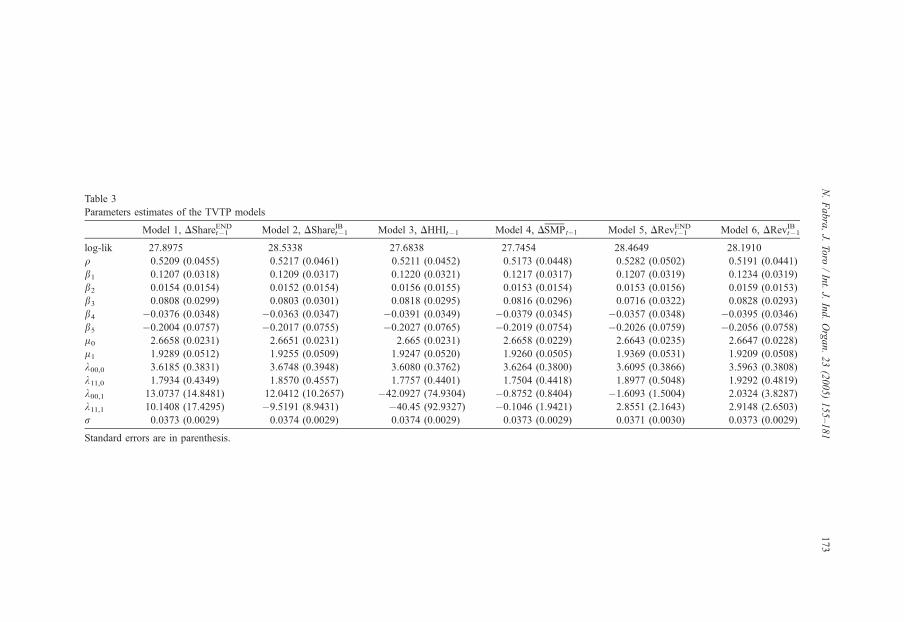
Table 3

Parameters estimates of the TVTP models

Model 1, DShareENDt�1 Model 2, DShareIBt�1 Model 3, DHHIt�1 Model 4, DSMP t�1 Model 5, DRevENDt�1 Model 6, DRevIBt�1

log-lik 27.8975 28.5338 27.6838 27.7454 28.4649 28.1910

q 0.5209 (0.0455) 0.5217 (0.0461) 0.5211 (0.0452) 0.5173 (0.0448) 0.5282 (0.0502) 0.5191 (0.0441)

b1 0.1207 (0.0318) 0.1209 (0.0317) 0.1220 (0.0321) 0.1217 (0.0317) 0.1207 (0.0319) 0.1234 (0.0319)

b2 0.0154 (0.0154) 0.0152 (0.0154) 0.0156 (0.0155) 0.0153 (0.0154) 0.0153 (0.0156) 0.0159 (0.0153)

b3 0.0808 (0.0299) 0.0803 (0.0301) 0.0818 (0.0295) 0.0816 (0.0296) 0.0716 (0.0322) 0.0828 (0.0293)

b4 �0.0376 (0.0348) �0.0363 (0.0347) �0.0391 (0.0349) �0.0379 (0.0345) �0.0357 (0.0348) �0.0395 (0.0346)

b5 �0.2004 (0.0757) �0.2017 (0.0755) �0.2027 (0.0765) �0.2019 (0.0754) �0.2026 (0.0759) �0.2056 (0.0758)

l0 2.6658 (0.0231) 2.6651 (0.0231) 2.665 (0.0231) 2.6658 (0.0229) 2.6643 (0.0235) 2.6647 (0.0228)

l1 1.9289 (0.0512) 1.9255 (0.0509) 1.9247 (0.0520) 1.9260 (0.0505) 1.9369 (0.0531) 1.9209 (0.0508)

k00,0 3.6185 (0.3831) 3.6748 (0.3948) 3.6080 (0.3762) 3.6264 (0.3800) 3.6095 (0.3866) 3.5963 (0.3808)

k11,0 1.7934 (0.4349) 1.8570 (0.4557) 1.7757 (0.4401) 1.7504 (0.4418) 1.8977 (0.5048) 1.9292 (0.4819)

k00,1 13.0737 (14.8481) 12.0412 (10.2657) �42.0927 (74.9304) �0.8752 (0.8404) �1.6093 (1.5004) 2.0324 (3.8287)

k11,1 10.1408 (17.4295) �9.5191 (8.9431) �40.45 (92.9327) �0.1046 (1.9421) 2.8551 (2.1643) 2.9148 (2.6503)

r 0.0373 (0.0029) 0.0374 (0.0029) 0.0374 (0.0029) 0.0373 (0.0029) 0.0371 (0.0030) 0.0373 (0.0029)

Standard errors are in parenthesis.

N.Fabra,J.

Toro

/Int.J.

Ind.Organ.23(2005)155–181

173

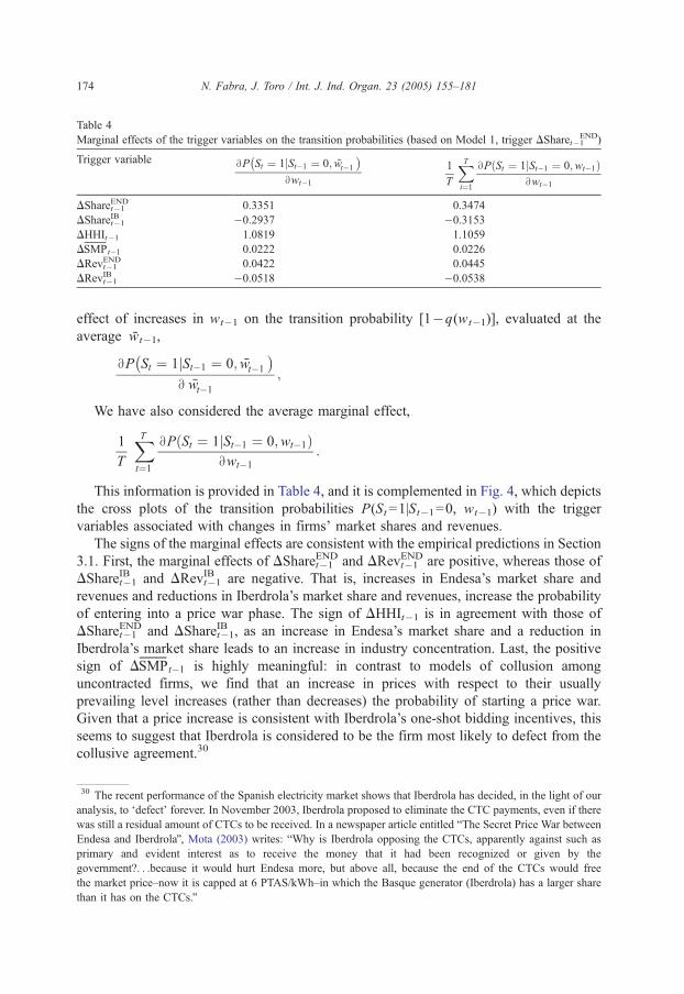
Table 4

Marginal effects of the trigger variables on the transition probabilities (based on Model 1, trigger DSharet�1END)

Trigger variable BP St ¼ 1jSt�1 ¼ 0; wt�1

� �Bwt�1

1

T

XTi¼1

BP St ¼ 1jSt�1 ¼ 0;wt�1ð ÞBwt�1

DShareENDt�1 0.3351 0.3474

DShareIBt�1 �0.2937 �0.3153

DHHIt�1 1.0819 1.1059

DSMP t�1 0.0222 0.0226

DRevENDt�1 0.0422 0.0445

DRevIBt�1 �0.0518 �0.0538


effect of increases in wt�1 on the transition probability [1�q(wt�1)], evaluated at the

average wt�1,

BP St ¼ 1jSt�1 ¼ 0; wt�1

� �B wt�1

;

We have also considered the average marginal effect,

1

T

XTt¼1

BP St ¼ 1jSt�1 ¼ 0;wt�1ð ÞBwt�1

:

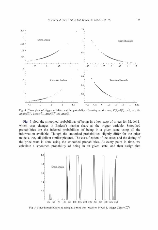
This information is provided in Table 4, and it is complemented in Fig. 4, which depicts

the cross plots of the transition probabilities P(St=1|St�1=0, wt�1) with the trigger

variables associated with changes in firms’ market shares and revenues.

The signs of the marginal effects are consistent with the empirical predictions in Section

3.1. First, the marginal effects of DShareENDt�1 and DRevENDt�1 are positive, whereas those of

DShareIBt�1 and DRevIBt�1 are negative. That is, increases in Endesa’s market share and

revenues and reductions in Iberdrola’s market share and revenues, increase the probability

of entering into a price war phase. The sign of DHHIt�1 is in agreement with those of

DShareENDt�1 and DShareIBt�1, as an increase in Endesa’s market share and a reduction in

Iberdrola’s market share leads to an increase in industry concentration. Last, the positive

sign of DSMPt�1 is highly meaningful: in contrast to models of collusion among

uncontracted firms, we find that an increase in prices with respect to their usually

prevailing level increases (rather than decreases) the probability of starting a price war.

Given that a price increase is consistent with Iberdrola’s one-shot bidding incentives, this

seems to suggest that Iberdrola is considered to be the firm most likely to defect from the

collusive agreement.30

30 The recent performance of the Spanish electricity market shows that Iberdrola has decided, in the light of our

analysis, to ddefectT forever. In November 2003, Iberdrola proposed to eliminate the CTC payments, even if there

was still a residual amount of CTCs to be received. In a newspaper article entitled bThe Secret Price War between

Endesa and IberdrolaQ, Mota (2003) writes: bWhy is Iberdrola opposing the CTCs, apparently against such as

primary and evident interest as to receive the money that it had been recognized or given by the

government?. . .because it would hurt Endesa more, but above all, because the end of the CTCs would free

the market price–now it is capped at 6 PTAS/kWh–in which the Basque generator (Iberdrola) has a larger share

than it has on the CTCs.Q

-.05 0 .05 .1

.025

.05

.075

.1

.125

Share Endesa

-.15 -.1 -.05 0 .05 .1 .15

.05

.1

.15

Share Iberdrola

-.5 0 .5 1 1.5

.1

.2

.3

Revenues Endesa

-.5 -.25 0 .25 .5 .75 1 1.25

.02

.04

.06

Revenues Iberdrola

Fig. 4. Cross plots of trigger variables and the probability of starting a price war, P(St=1|St�1=0, wt), for

DShareENDt�1 , DShareIBt�1, DRev

ENDt�1 and DRevIBt�1.


Fig. 5 plots the smoothed probabilities of being in a low state of prices for Model 1,

which uses changes in Endesa’s market share as the trigger variable. Smoothed

probabilities are the inferred probabilities of being in a given state using all the

information available. Though the smoothed probabilities slightly differ for the other

models, they all deliver similar pictures. The classification of the states and the dating of

the price wars is done using the smoothed probabilities. At every point in time, we

calculate a smoothed probability of being in an given state, and then assign that

25 50 75 100 125 150 175 200 225 250 275 300 325 350

0.2

0.4

0.6

0.8

1.0

Share Endesa

Fig. 5. Smooth probabilities of being in a price war (based on Model 1, trigger DShareENDt�1 ).

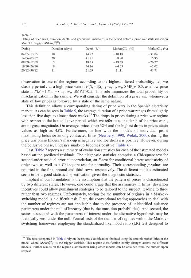
Table 5

Dating of price wars, duration, depth, and generators’ mark-ups in the period before a price war starts (based on

Model 1, trigger DSharet�1END)

Dating Duration (days) Depth (%) MarkupENDt�1 (%) MarkupIBt�1 (%)

04/05–13/05 10 44.27 �10.18 �31.04

14/06–03/07 20 41.21 8.80 15.95

08/09–12/09 5 18.75 �19.38 �26.77

19/10–26/10 8 34.16 �4.63 �2.02

20/12–30/12 11 21.69 21.11 41.71


observation to one of the regimes according to the highest filtered probability, i.e., we

classify period t as a high-price state if P(St=1|St�1=st�1, wt, SMPt)b0.5, as a low-price

state if P(St=1|St�1=st�1, wt, SMPt)N0.5. This rule minimizes the total probability of

misclassification in the sample. We will consider the definition of a price war whenever a

state of low prices is followed by a state of the same nature.

This definition allows a corresponding dating of price wars in the Spanish electricity

market. As can be seen in Table 5, the average duration of a price war ranges from slightly

less than five days to almost three weeks.31 The drops in prices during a price war regime

with respect to the last collusive period–which we refer to as the depth of the price war–,

are of great magnitude. On average, prices drop 32% and the highest drops in prices attain

values as high as 45%. Furthermore, in line with the models of individual profit

maximizing behavior among contracted firms (Newbery, 1998; Wolak, 2000), during the

price war phase Endesa’s mark-up is negative and Iberdrola’s is positive. However, during

the collusive phase, Endesa’s mark-up becomes positive (Table 6).

Last, Table 7 reports a summary of evaluation statistics for each of the estimated models

based on the predicted residuals. The diagnostic statistics comprise a Chi-square test for

second-order residual error autocorrelation, an F-test for conditional heteroscedasticity of

order two, as well as a Chi-square test for normality. Their corresponding p-values are

reported in the first, second and third rows, respectively. The different models estimated

seem to be a good statistical specification given the diagnostic statistics.

Implicit in our formulation is the assumption that the pattern of prices is characterized

by two different states. However, one could argue that the asymmetry in firms’ deviation

incentives could allow punishment strategies to be tailored to the suspect, leading to three

rather than two regimes. Unfortunately, testing for the number of regimes in a Markov-

switching model is a difficult task. First, the conventional testing approaches to deal with

the number of regimes are not applicable due to the presence of unidentified nuisance

parameters under the null of linearity (that is, the transition probabilities). And second, the

scores associated with the parameters of interest under the alternative hypothesis may be

identically zero under the null. Formal tests of the number of regimes within the Markov-

switching framework employing the standardized likelihood ratio (LR) test designed to

31 The results reported in Table 5 rely on the regime classification obtained using the smooth probabilities of the

model where DShareENDt�1 is the trigger variable. This regime classification hardly changes across the different

models. Further results on the regime classification using other models can be obtained from the authors upon

request.

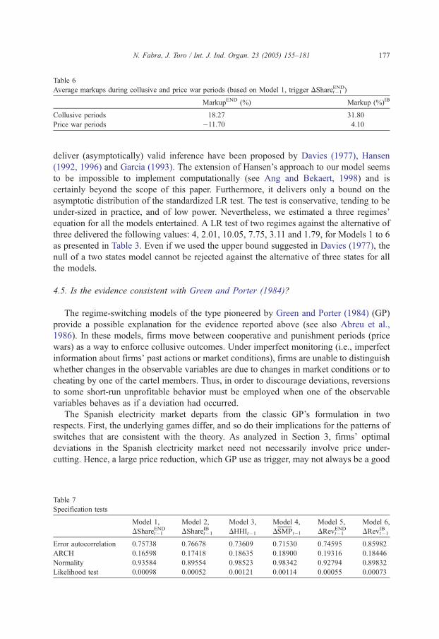
Table 6

Average markups during collusive and price war periods (based on Model 1, trigger DShareENDt�1 )

MarkupEND (%) Markup (%)IB

Collusive periods 18.27 31.80

Price war periods �11.70 4.10


deliver (asymptotically) valid inference have been proposed by Davies (1977), Hansen

(1992, 1996) and Garcia (1993). The extension of Hansen’s approach to our model seems

to be impossible to implement computationally (see Ang and Bekaert, 1998) and is

certainly beyond the scope of this paper. Furthermore, it delivers only a bound on the

asymptotic distribution of the standardized LR test. The test is conservative, tending to be

under-sized in practice, and of low power. Nevertheless, we estimated a three regimes’

equation for all the models entertained. A LR test of two regimes against the alternative of

three delivered the following values: 4, 2.01, 10.05, 7.75, 3.11 and 1.79, for Models 1 to 6

as presented in Table 3. Even if we used the upper bound suggested in Davies (1977), the

null of a two states model cannot be rejected against the alternative of three states for all

the models.

4.5. Is the evidence consistent with Green and Porter (1984)?

The regime-switching models of the type pioneered by Green and Porter (1984) (GP)

provide a possible explanation for the evidence reported above (see also Abreu et al.,

1986). In these models, firms move between cooperative and punishment periods (price

wars) as a way to enforce collusive outcomes. Under imperfect monitoring (i.e., imperfect

information about firms’ past actions or market conditions), firms are unable to distinguish

whether changes in the observable variables are due to changes in market conditions or to

cheating by one of the cartel members. Thus, in order to discourage deviations, reversions

to some short-run unprofitable behavior must be employed when one of the observable

variables behaves as if a deviation had occurred.

The Spanish electricity market departs from the classic GP’s formulation in two

respects. First, the underlying games differ, and so do their implications for the patterns of

switches that are consistent with the theory. As analyzed in Section 3, firms’ optimal

deviations in the Spanish electricity market need not necessarily involve price under-

cutting. Hence, a large price reduction, which GP use as trigger, may not always be a good

Table 7

Specification tests

Model 1,

DShareENDt�1

Model 2,

DShareIBt�1

Model 3,

DHHIt�1

Model 4,

DSMPt�1

Model 5,

DRevENDt�1

Model 6,

DRevIBt�1

Error autocorrelation 0.75738 0.76678 0.73609 0.71530 0.74595 0.85982

ARCH 0.16598 0.17418 0.18635 0.18900 0.19316 0.18446

Normality 0.93584 0.89554 0.98523 0.98342 0.92794 0.89832

Likelihood test 0.00098 0.00052 0.00121 0.00114 0.00055 0.00073


signal of cheating; accordingly, it is not clear whether it should be expected to trigger price

wars.

The other difference with respect to GP is related to the information available to the

Spanish electricity producers. In particular, in contrast with GP who assume that only

prices but not quantities are observed, the Spanish electricity producers observe both

aggregate quantities and prices at gate-closure. Nevertheless, this does not imply that the

Spanish electricity producers may perfectly detect their rivals’ potential deviations. First,

the generation coming from the must-run resources (mainly, cogeneration and renewables)

is not known. And second, firms’ available capacities are subject to random shocks, out of

firms’ control (e.g. capacities may suffer random outages, or be increased due to an excess

of run of the river hydro power). This implies that a firm’s departure from any agreed upon

market share may have resulted either from cheating by a rival, or from any of those

random and unobservable factors cited above. Therefore, even if the sources of imperfect

information differ, the Spanish electricity producers are faced with the same kind of signal

extraction problem as in a GP type of model.32

To assess whether the evidence is consistent with GP, we proceed by comparing our

empirical findings with their main predictions. First, the fact that two distinct price levels

characterize the time series of prices in the Spanish electricity market confirms GP’s

prediction that price wars should be observed in equilibrium. Second, the statistical

significance of the trigger variables is consistent with GP’s prediction that price wars must

be linked to movements in the trigger variables. Third, since the effects of the triggers

coincide with the theoretical findings, GP’s prediction that price wars should be more

likely to occur when the trigger variables move as if a deviation had taken place is

confirmed. Unfortunately, the lack of data on individual bids does not allow us to test GP’s

prediction that deviations should not take place in equilibrium. Nevertheless, the

information contained in Table 5 may shed some light on this issue. It shows that the

behavior of firms’ mark-ups in the period that triggers the price war is not homogenous

across the different price wars, probably suggesting that deviations are not taking place (or

at least, not always in the same direction).

Having said all this, there are other reasons that indicate caution regarding

interpretation of the evidence as support for GP’s model. The incentive structure

embedded in GP’s model requires a high degree of rationality, which cannot be reasonably

expected in a market that has only recently started to operate. Furthermore, firms’ optimal

deviations in GP’s model are symmetric, implying that movements in the trigger variables

do not convey any information about the potential deviator. In our case, the asymmetry in

firms’ deviation incentives should in principle allow punishments to be tailored to the

suspect. The fact that a three-state model is rejected in our data contradicts the use of an

32 There is an alternative branch of the literature on collusion in markets subject to variable demand, exemplified

by the models of Rotemberg and Saloner (1986) and Haltiwanger and Harrington (1991). In these models, which

assume perfect monitoring, price wars do not arise as equilibrium phenomena. Instead, the sustainability of

collusion is maintained through smoother price adjustments, which depend on current or future demand

conditions. However, we believe that perfect monitoring is an unrealistic assumption in the Spanish electricity

market.


optimal collusive device, and hence casts some doubts on the applicability of GP’s model

to our data set.

Indeed, there could be several alternative explanations, other than collusion, for the

phenomena that we observe in the Spanish data. For instance, if firms were not pursuing

collusive strategies, the existence of periods of low prices could be accounted for by mixed

strategy pricing or by the lack of coordination on the multiple price equilibria (see von der

Fehr and Harbord, 1993). However, if this were the case, there should be no reason to

observe such a persistence in each price state as we observe in the data. Furthermore, there

should not be a systematic relationship between the trigger variables and the occurrence of

price wars, i.e., their coefficients should be non-significant.

5. Conclusions

We have analyzed the dynamic exercise of market power in the Spanish electricity

market during 1998 using daily observations on demand, prices and other variables that

allow us to obtain accurate marginal costs estimates at the firm level. The Spanish

electricity market has interesting institutional features that make this analysis relevant both

for public policy, as well as from a methodological perspective.

As in all decentralized electricity markets, trading in the Spanish electricity market

takes place through a series of daily auctions. Both theory and experience suggest that the

daily repetition of auctions may have a dramatic effect on market performance, as it allows

firms to learn to coordinate their strategies and hence compete less aggressively with each

other over time, through collusive agreements. However, unlike other markets, collusion in

the Spanish electricity market need not result in high price-cost margins, precisely because

the Spanish electricity producers are entitled to earn some regulatory payments, which are

computed in a similar fashion as bContracts for DifferencesQ. The theoretical predictions

imply that an over-contracted firm may find it in its private interest to reduce prices, as this

strategy may lead to an increase in its contract revenues that more than compensates for

the reduction in prices. Thus, even in a static context, the value of firms’ mark-ups does

not provide a precise measure of firms’ ability to exercise market power. To overcome this

difficulty, our analysis has exploited the movements in prices, firms’ market shares and

revenues in order to infer firms’ ability to exercise market power in a dynamic context.

The performance of the Spanish electricity market during 1998 is not consistent with

the predictions of models of individual profit maximizing behavior. In particular, the over-

contracted firm should have produced at prices below marginal costs, and the movements

in prices should have been fully explained by changes in demand and cost conditions.

These observations have led us to conjecture that the Spanish electricity producers may

have been engaged in some kind of tacit agreement that distorted market outcomes from

the predictions of the theories of individual profit maximizing behavior.

Our analysis has been designed to test the above conjecture. In order to identify the

plausible triggers that firms could have used to support collusion, we have first identified

firms’ optimal deviations from a model of joint-profit maximizing behavior. This model

predicts that price wars should be triggered when the market share and revenues of the

under-contracted firm decrease, and those of the over-contracted firm increase. We have


tested these predictions empirically by modelling the time series of prices as a Markov-

switching process in the mean, with time-varying transition probabilities that depend on

changes in firms’ market shares, revenues, and market prices. The results confirm that the

time series of prices is characterized by two distinct price levels. Furthermore, most of the

triggers considered appear to be significant and report the same signs as those predicted by

the theory. These results offer further support to the claim that the way in which the CTCs

have been computed has had an important impact in firms’ bidding incentives.

Acknowledgments

Special thanks are due to Giulio Federico, Soren Johansen and Massimo Motta. James

Bushnell, Kristi Green, Inigo Herguera, Ed Kahn, Matt Shum, Steve Puller and seminar

participants at the University of California Energy Institute (2003 POWER Conference),

Universidad Carlos III de Madrid (2002 EARIE Conference), and Universidad

Complutense de Madrid (February 2003) provided helpful suggestions. Detailed

comments by two anonymous referees and the Editor, Igal Hendel, also contributed to

improve the paper. Antonio Jesus Sanchez provided excellent research assistance. All

errors remain our own responsibility. Research reported in this paper was partly carried out

while the first author was at the IDEI (Toulouse) and the UCEI (Berkeley) and the second

author was at Oxford University; we are indebted to them for their hospitality and

encouragement.

References

Abreu, D., Pierce, D., Stacchetti, E., 1986. Optimal Cartel equilibria with imperfect monitoring. Journal of

Economic Theory 39, 251–269.

Ang, A., Bekaert, G., 1998. Regime Switches in Interest Rates. Working Paper, Stanford University.

Arocena, P., Kuhn, K.-U., Regibeau, P., 1999. Regulatory reform in the Spanish electricity industry: a miss

opportunity for competition. Energy Policy, 387–399.

Borenstein, S., Bushnell, J., 1999. An empirical analysis of the potential for market power in California’s

electricity industry. Journal of Industrial Economics XLVII (3), 285–323.

Borenstein, S., Bushnell, J., Wolak, F., 2002. Measuring market inefficiencies in California’s restructured

wholesale electricity market. American Economic Review 92 (5), 1376–1405.

Bushnell, J., 2003. A mixed complementarity model of hydro-thermal electricity competition in the Western U.S.

Operations Research 51 (1).

CNE, 2000. El Funcionamiento del Mercado Electrico en el Ano 1998. Technical report, Comision Nacional de la

Energıa, Madrid.

Crampes, C., Fabra, N., in press. The Spanish electricity industry: plus ca change. . ., Energy Journal.

Davies, R.B., 1977. Hypothesis testing when a nuisance parameter is present only under the alternative, 64,

247–254.

Ellison, G., 1994. Theories of Cartel stability and the joint executive committee. Rand Journal of Economics 25,

37–57.

Engle, R.F., Hendry, D.F., Richard, J., 1983. Exogeneity. Econometrica 51, 277–304.

Fabra, N., 2003. Tacit collusion in repeated auctions: uniform versus discriminatory. Journal of Industrial

Economics L1 (3), 271–293.

Fabra Utray, J., 2004. Un Mercado Para la Electricidad: Liberalizacion o Regulacion? Marcial Pons, Madrid.


Filardo, A., 1994. Business-cycle phases and their transitional dynamics. Journal of Business Economics and

Statistics 12, 299–308.

Garcia, R., 1993. Asymptotic null distribution of the likelihood ratio test in Markov switching models. Technical

report, Universite de Montreal.

Green, R., Newbery, D., 1992. Competition in the British electricity spot market. Journal of Political Economy

100, 929–953.

Green, E.J., Porter, R.H., 1984. Noncooperative collusion under imperfect price information. Econometrica 52

(1), 87–100.

Haltiwanger, J., Harrington, J., 1991. The impact of cyclical demand movements on collusive behavior. Rand

Journal of Economics 22, 89–106.

Hamilton, J.D., 1989. A new approach to the economic analysis of nonstationary time series and the business

cycle. Econometrica 57, 357–384.

Hansen, B.E., 1992. The likelihood ratio test under non-standard conditions: testing the Markov Switching Model

of GNP. Journal of Applied Econometrics 7, S61–S82.

Hansen, B.E., 1996. Erratum: the likelihood ratio test under non-standard conditions: testing the Markov

Switching Model of GNP, 11, 195–199.

Joskow, P., Kahn, E., 2002. A quantitative analysis of pricing behavior in California’s wholesale electricity market

during Summer 2000. The Energy Journal 22 (4), 1–35.

Marın, P., Garcıa-Dıaz, A., 2003. Strategic bidding in electricity pools with short-lived bids: an application to the

Spanish market. International Journal of Industrial Organization 21, 201–222.

Mota, J., 2003. La Guerra Secreta Entre Endesa e Iberdrola. El Pais Negocios 18 (November).

Newbery, D., 1998. Competition, contracts, and entry in the electricity spot market. Rand Journal of Economics

29 (4), 726–749.

Patrick, R., Wolak, F., 1997. The impact of market rules and market structure on the price determination process

in the England and Wales electricity market. Working Paper, PWP-047, University of California, POWER.

Puller, S., 2000. Pricing and firm conduct in California’s deregulated electricity market, PWP-080. UCEI,

California.

Rotemberg, J., Saloner, G., 1986. A supergame theoretic model of price wars during booms. American Economic

Review 70, 390–407.

von der Fehr, N., Harbord, D., 1993. Spot market competition in the UK electricity industry. The Economic

Journal 103, 531–546.

Wolak, F., 2000. An empirical analysis of the impact of hedge contracts on bidding behavior in a competitive

electricity market. International Economic Journal 14 (2), 1–39.

Wolak, F., 2003. Measuring unilateral market power in wholesale electricity markets: the California market,

1998–2000. American Economic Review, Papers and Proceedings May, 425–430.

Wolfram, C., 1998. Strategic bidding in a multi-unit auction: an empirical analysis of bids to supply electricity in

England and Wales. Rand Journal of Economics 29 (4), 703–725.

Wolfram, C., 1999. Measuring duopoly power in the British spot market. American Economic Review 89,

805–826.

Documents

Price wars and collusion in the Spanish electricity market