Prices, Wages and the U.S. NAIRU in the 1990s

January 2001

(Revised June 2001)

Douglas Staiger Dartmouth College

and the National Bureau of Economic Research

James H. Stock Kennedy School of Government, Harvard University

and the National Bureau of Economic Research

and

Mark W. Watson* Department of Economics and Woodrow Wilson School, Princeton University

and the National Bureau of Economic Research

*Prepared for the conference on the Sustainable Employment Initiative, sponsored by the Century and Russell Sage Foundations. We thank David Autor for helpful discussions and William Dickens and Robert Solow for detailed comments on an earlier version of this paper.

Prices, Wages and the U.S. NAIRU in the 1990s

ABSTRACT

Using quarterly macro data and annual state panel data, we examine various explanations of the low rate of price inflation, strong real wage growth, and low rate of unemployment in the U.S. economy during the late 1990s. Many of these explanations imply shifts in the coefficients of price and wage Phillips curves. We find, however, that once one accounts for the univariate trends in the unemployment rate and in the rate of productivity growth, these coefficients are stable. This suggests that many explanations, such as persistent beneficial supply shocks, changes in firms’ pricing power, changes in price expectations arising from shifts in Fed policy, and changes in wage setting behavior miss the mark. Rather, we suggest that explanations of movements of wages, prices and unemployment over the 1990s, and indeed over the past forty years, must focus on understanding the univariate trends in the unemployment rate and in productivity growth and, perhaps, the relation between the two. Douglas Staiger Department of Economics Dartmouth College Rockefeller Hall, Room 322 Hanover, NH 03755-3514 James H. Stock Kennedy School of Government Harvard University Cambridge, MA 02138 Mark W. Watson Department of Economics Princeton University Princeton, NJ 08544 Keywords: Phillips Curve, natural rate, productivity JEL Classification: E31, E50

1

1. Introduction

One of the most salient features of the U.S. expansion in the second half of the

1990s was the combination of low price inflation, strong real wage growth, and low and

falling unemployment. On its face, this runs counter to the postwar U.S. experience that

periods of low unemployment and strong wage growth are associated with rising rates of

inflation. This paper undertakes an empirical investigation of the extent to which

changes in price setting behavior, changes in wage setting behavior, and fundamental

changes in product and labor markets led to this happy coincidence.

The facts are summarized in figure 1. Figure 1a is a scatterplot of the change in

the annual rate of price inflation, as measured by the GDP deflator, vs. the unemployment

rate in the previous year, from 1960 – 1999; for example, the point labeled “98” indicates

the unemployment rate in 1998 and the change in the rate inflation from 1998 to 1999.

Figure 1b is a comparable scatterplot, except that the series on the vertical axis is the

annual percentage growth rate of real wages, as measured by compensation per hour in

the nonfarm business sector, deflated by the GDP deflator. The regression line estimated

using data from 1960-1992 is plotted in both figures. These regression lines are simple

estimates of the price and wage Phillips curves. The NAIRU is defined to be the value of

the unemployment rate at which the price regression predicts no change in inflation,

which corresponds to the intersection of the regression line and the horizontal line in

figure 1a. Alternatively, the wage-based NAIRU is the value of the unemployment rate

at which the wage regression line predicts real wage growth that coincides with the

2

growth in labor productivity, which is given by the intersection of the regression line and

the horizontal line in figure 1b.

Three features are evident from these scatterplots. First, both the wage and price

Phillips curves reflect a negative correlation between the unemployment rate in one year

and inflation in the next: the correlation in figure 1a for the 1960 – 1992 sample is -0.55,

and the correlation in figure 1b is -0.65. Second, the data for 1993 – 1999 (highlighted in

the figure) are peculiar, relative to the earlier data: although unemployment fell from

7.5% in 1992 to 4.1% in 1999, the rate of price inflation was essentially constant over

this period (it fell by an average of 0.1% per year). Third, from 1993 to 1999 real wages

increased substantially: real wages grew by an average of 1.5% over this period,

consistent with little if any shift in the NAIRU in this wage scatterplot and, if anything, a

steeper wage Phillips curve regression line.

The theories that have been proposed to explain these events fall into two groups:

theories in which “The Phillips curve is alive and well but…” and those that proclaim

that “the Phillips curve is dead.”

Most of the proposed theories are in the “alive and well but…” group. According

to these theories, the price Phillips curve – the regression line in figure 1a – continues to

have a negative slope, but it has been shifting inwards. Such a shift is indicated by the

arrow and dashed line in figure 1a. Similarly, the strong growth of real wages in the late

1990s in figure 1b is attributed by these theories to the surge in productivity: workers are

reaping the rewards of using more powerful tools. The differences among these theories

arise in the particulars of how they explain the inward shift of the price inflation Phillips

curve: some focus on price setting behavior of firms, others focus on labor markets,

3

while others suggest that we simply have been the lucky recipients of favorable supply

shocks (falling energy prices and favorable terms of trade shocks).

The theories that focus on pricing behavior have several variants. One is that

globalization has increased competition in the product market, thereby squeezing

markups and yielding one-time reductions in markups and prices (e.g. Brayton et. al.

[1999]). Similar arguments can be made about the possible effect of the Internet on price

competition for some goods. A different argument is that the credibility of the

commitment of the Federal Reserve Board to controlling inflation has increased, and that

this has had the effect of reducing expected inflation which in turn moderates actual price

increases posted by producers.

The theories that focus on labor markets suggest that the source of the inward

shift in the Phillips curve lies with a decline in the natural rate of unemployment. Several

such theories are surveyed and analyzed empirically in Katz and Krueger (1999). Some

emphasize changes in how people look for work (using temporary help firms, using the

Internet, etc.). Others emphasize changes in the composition of the work force, including

the aging of the workforce as the baby boom enters an age traditionally associated with

high degrees of labor force attachment, the entry of “welfare mothers” into the workforce

as a consequence of welfare reform, and the removal of many marginal workers from the

workforce either because of incarceration (Katz and Krueger [1999]) or because of

relaxed Social Security Disability Insurance (SSDI) provisions (Autor and Duggan

[2000]).

Finally, some of these theories stress the role of good luck. For much of the

1990s, energy prices were declining and the U.S. enjoyed a strong dollar. Gordon (1998)

4

explored these sources in detail, and concluded that they explain part, but far from all, of

the price inflation/unemployment puzzle of the 1990s.

In contrast, “The Phillips Curve is dead” theories interpret the 1990s not as an

inward drift in the Phillips curve, but rather as a fundamental change in the relation

between unemployment and inflation. According to these theories, it is the slope of the

Phillips curve that has shifted, not the intercept: the Phillips curve now is the dotted line

in Figure 1a, which was fit to the data from 1993 – 1999. This curve has a slope of zero.

This more radical interpretation requires more radical theories. The popular press

versions of these theories stress that increased price competition in the new economy

prevents firms from responding to market tightness by increasing prices, thereby

eliminating any relation between measures of aggregate activity, such as unemployment,

and changes in the rate of price inflation.

Subtler versions of these theories involve nonlinearities in firm behavior when

inflation is low. Akerlof, Dickens and Perry (1996) suggest that reluctance by firms to

give negative nominal wage cuts means that steady state hiring depends on the rate of

inflation; in particular, the equilibrium unemployment rate falls when inflation falls.

Taylor (2000) develops a different theory of state-dependence of the NAIRU; in his

model, low inflation itself leads firms to expect reduced pricing power, which in turn

contributes to reduced inflation and reduces the sensitivity of inflation to growth in

demand. Akerlof, Dickens and Perry (2000) provide a model of price setting in which

some firms find it convenient to predict zero inflation as long as inflation is low,

permitting the unemployment rate to be persistently low without igniting inflation.

Empirically, this is the same thing as the NAIRU falling when the inflation rate gets low.

5

In all three of these models, the NAIRU is not permanently low, but rather its low value

is contingent upon the monetary authority holding down inflation.

This paper has two objectives. The first, more modest one is to document the

shifts in Figure 1. To a considerable extent, this entails updating earlier estimates of

Phillips curves and NAIRUs along the lines of Staiger, Stock and Watson (1997a, 1997b)

and Gordon (1998). The second, more ambitious objective is to provide new evidence,

based on quarterly macro data and on a panel of annual data for U.S. states from 1979 –

1999, that helps us to parse the theories outlined above or, at least, to rule out some

families of theories.

We do this by addressing three specific questions. First did the Phillips curve

break down in the 1990s, or did it simply shift, with a new and evolving NAIRU? That

is, which class of theories – “the Phillips curve is dead” or “the Phillips curve is alive,

but…” has more empirical support? We conclude that the weight of the evidence

supports the “alive but…” group of theories: the evidence suggests that the price Phillips

curve has shifted in, not flattened out.

This leads to the second question: why has the price Phillips curve shifted in?

That is, does the empirical evidence help to distinguish between the many theories of the

inward drift in the price Phillips Curve? In our view, the weight of the empirical

evidence points towards explanations that involve special features in labor markets. The

macro evidence suggests that changes in price setting behavior cannot explain the broad

stability of the relation between price inflation and measures of economic activity.

Rather, the explanation for the shifting unemployment Phillips curve seems to lie in

declines in the univariate trend rate of unemployment.

6

The third question, then, is whether labor productivity gains during the 1990s can

explain the apparently aberrant recent behavior of real wages in Figure 1b. That is, is the

wage Phillips curve as resilient empirically as the price Phillips curve, once we have

accounted for productivity? Our answer is yes: adjusting for trend labor productivity

gains accounts for the discrepancies that otherwise appear between the price and wage

Phillips curves.

In short, once one allows for the univariate trends in the unemployment rate and

the rate of productivity growth, the 1990s present no wage or price puzzles. Backward

looking price Phillips curves are stable when the unemployment rate is specified as a gap,

that is, as the deviation from its univariate trend value. Similarly, wage Phillips curves

are stable when wages are adjusted for changes in trend productivity growth and when

the regressions are specified using activity gaps. This implies that theories of the 1990s

that focus on favorable supply shocks, changes in pricing power of firms and markups, or

changes in the negotiating power of labor all miss the mark, for these theories imply

persistent errors and/or coefficient instability that we fail to find. Rather, this evidence

points to underlying economic forces that change the univariate trends of the

unemployment rate and the growth rate of productivity. Unfortunately, our regressions

using the state data fail to isolate any economic or demographic determinants of the trend

unemployment rate.

The plan of the paper is as follows. Sections 2 – 5 analyze quarterly U.S. macro

data from 1960 – 2000. We begin in section 2 by estimating the long-run trends in the

macro data and discussing how we estimate output gaps. Section 3 addresses issues of

econometric specification and estimation of the price and wage Phillips curves and

7

associated time-varying NAIRUs (TV-NAIRUs). These Phillips curves are specified

using output gaps, which are the difference between the output measure and its low

frequency univariate trend component. As Hall (1999) and Cogley and Sargent (2001)

argue, the low frequency trend component can be thought of as an estimate of the natural

rate of unemployment; thus this approach allows separate identification of the NAIRU

and the natural rate. Section 4 reports empirical price Phillips relations estimated both

with the unemployment rate gap and with gaps based on other measures of economic

activity. Consistent with the findings in Staiger, Stock and Watson (1997a), Stock (1998)

and Stock and Watson (1999b), we find stability and predictive content in these broader

measures, which suggests that the “Phillips curve is dead” theories are premature. In

section 5, we turn to wage Phillips curves and examine the role of productivity gains in

explaining the recent rise in real wages.

Sections 6-9 focus on the state panel data. Although some authors in this

literature have used state level data (notably Katz and Krueger [1999] and Lerman and

Schmidt [1999]), their use has been limited and we are able to consider a large number of

new variables and, accordingly, to use the state data to examine the various theories.

Specifications and econometric issues, including our instrumental variables (IV) method

for alleviating errors-in-variables bias arising from using the state data, are discussed in

section 6. The data set is described in section 7, and benchmark results are presented in

section 8. Section 9 reports results of using additional variables to explore the stability of

the Phillips curve and to examine theories about sources of shifts in the NAIRU.

Conclusions are summarized in section 10.

8

A remark on terminology is in order before proceeding. In conventional usage,

the “NAIRU” is the rate of unemployment consistent with price inflation remaining

constant; the “NAWRU” is the rate of unemployment consistent with wage inflation

remaining constant; and the “NAIRCU” is the rate of capacity utilization consistent with

price inflation remaining constant. In this paper, we consider both wage and price

inflation and consider other activity indexes, including building permits and

demographically adjusted unemployment. We could, then, report TV-NAWRCUs, TV-

NAIRBPs, TV-NAWRDUs, and so on. But we do not find these acronyms helpful.

Instead, we shall call them all TV-NAIRUs and, when needed, shall add specificity

through the use of adjectives.

2. Trends in the Macro Data

2.1 Method for Estimating Univariate Trends and Constructing Gaps

Let yt be a quarterly time series, and let *ty denote its trend. Unless explicitly

noted otherwise, *ty is estimated by passing yt through a two-sided low pass filter, with a

cutoff frequency corresponding to 15 years. Essentially, this estimates *ty as a long two-

sided weighted moving average of yt with weights that sum to one. Estimates of the trend

at the beginning and end of the sample are obtained by extending (padding) the series

with autoregressive forecasts and backcasts of yt, constructed from an estimated AR(4)

model (with a constant term) for the first difference of yt. The “gap” value of yt, gty , is

defined to be the deviation of yt from its trend value; that is, gty = yt – *

ty . Thus, the

9

trend value of the unemployment rate is the value of the unemployment rate resulting

from the low pass filter, and the unemployment gap is the difference between the actual

unemployment rate and the long run trend in unemployment.

2.2 Description of the Aggregate U.S. Data

The U.S. data are quarterly from 1959:I to 2000:II. The primary price measure is

the GDP deflator, but in our sensitivity analysis we also consider the personal

consumption expenditure (PCE) deflator, the Consumer Price Index (CPI) and the

deflator for the nonfarm business component of GDP . All rates of inflation are

computed as πt = 400ln(Pt/Pt-1), where Pt is the level of the price index in quarter t.

Several measures of wages are used. Our primary measure is compensation per

hour in the nonfarm business sector. For sensitivity checks, we also consider the

Employment Cost Index (both total compensation and wages and salaries only), average

hourly earnings of nonagricultural production workers, and compensation per hour in

manufacturing. Wage growth rates are computed as ωt = 400ln(Wt/Wt-1), where Wt is the

level of the wage index.

Labor productivity is measured by output per hour of all workers in the nonfarm

business sector, except when we consider compensation per hour in manufacturing, in

which case labor productivity is measured by output per hour of all workers in

manufacturing.

Economic activity is variously measured by the total unemployment rate, a

demographically adjusted unemployment rate, the rate of capacity utilization, and

housing starts (building permits). The demographically adjusted unemployment rate was

10

constructed as weighted average of the unemployment rates for 14 age-gender categories

(ages 16-19, 20-24, 25-34, 35-44, 45-54, 55-64, 65+, each by male/female), weighted by

the shares of each age group in the 1985 labor force.

Supply shock variables in the Phillips curve regressions are Gordon’s (1982) price

control series, the relative price of food and energy, and exchange rates.

Data sources for all series are given in the Data Appendix.

2.3 Low Frequency Properties of the Data

Figure 2 presents quarterly time series data and their estimated trends for (a) price

inflation (GDP deflator), (b) wage inflation (compensation per hour), (c) real wage

growth (compensation per hour deflated by GDP deflator inflation), (d) labor productivity

growth, (e) the unemployment rate, (f) the demographically adjusted unemployment rate,

(g) building permits (housing starts), and (h) the rate of capacity utilization. The “gaps”

of each of these variables is the difference between the quarterly data and their estimated

trends. Table 1 shows the sample mean of each of these series over each of the four

decades in the sample and, as a measure of persistence in the series, a 95% confidence

interval for the largest root in a univariate autoregression with six lags.

Figure 2 and table 1 show several important features of these data. First consider

wages, prices and productivity. Figures 2a and 2b show substantial low-frequency (trend)

variability in price and nominal wage inflation. As shown in table 1, this low frequency

variability leads to confidence intervals for the largest AR root that range from 0.90 to

1.02 (which, notably, include a unit AR root). Nominal wage growth less productivity

growth is also persistent: the confidence interval for its largest AR root is 0.81 to 1.00.

11

In contrast, real wage growth and, especially, real wage growth less productivity

growth are considerably less persistent, and 95% confidence intervals for their largest AR

roots do not include unity. Still, the decade-long averages in real wages show

considerable variability, and the ratio of the largest to the smallest decadal average varies

by a factor of more than 2.5. Table 1 shows that these decade-long changes in real wage

growth rates are broadly consistent with movements in the growth of labor productivity:

real wage growth and labor productivity growth were both high in the 60’s, low in the

80’s, etc. The relationship is stronger when wages, prices and productivity all pertain to

the non-farm business sector than when the GDP deflator is used to construct real wages.

Average real wage growth adjusted for productivity changes little over the decades in the

sample.

Formally, the hypothesis of a unit root in productivity is rejected, which taken

literally indicates that productivity growth is stationary. This characterization, however,

does not allow for the possibility of slowly changing mean productivity growth rates that

lie at the heart of the new economy debate. From a statistical point of view, if there is a

highly persistent component of productivity growth but its variance is small relative to

variations induced by cyclical movements and measurement error, then it will be difficult

to detect and the series can spuriously appear to be stationary.

These results are consistent with price inflation and nominal wage inflation

adjusted for productivity growth sharing a common stochastic trend that disappears from

real wage growth adjusted for productivity growth. In the terminology of integration and

cointegration, this suggests that price inflation is integrated of order 1 (is I(1)), wage

inflation less productivity growth is I(1), and real wage growth less productivity growth

12

is I(0); that is, price inflation is cointegrated with wage inflation less productivity

growth, with a cointegrated vector of (1, -1).1

Consistent with this specification, the level of productivity adjusted real wages

(equivalently, the “markup” or “labor’s share”) appears to be I(1). When real wages are

computed using the GDP deflator, there is a marked downward trend in the markup, but

when the GDP deflator is replaced by the non-farm business deflator, much of the trend

disappears. In either case, the series is very persistent and a unit autoregressive root

cannot be rejected.

The unemployment rate, building permits (housing starts) and capacity utilization

are shown in Figures 2e-2h. The unemployment rate trend exhibits large variability

(Figure 2e), and most of this variability remains in the demographically adjusted

unemployment rate (Figure 2f). In contrast, the trends in building permits and capacity

utilization (Figures 2g and 2h) show much less variability. Table 1 indicate that the

unemployment rate series are much more persistent than the building permits and

capacity utilization series: unit autoregressive roots cannot be rejected for both

unemployment series, but can be rejected for both building permits and capacity

utilization.

In summary, these statistics suggest that price inflation and nominal wage

inflation, adjusted for productivity growth, are cointegrated. Real wages and productivity

growth move together at low frequencies, although these movements are small in

magnitude compared with the noise and cyclical movements in these series. The

1 Application of the Horvath-Watson (1995) test rejects the null hypothesis of noncointegration of these two series against the alternative that they are cointegrated with the cointegrating vector of (1, -1) at the 1% significance level (the test statistic was computed with four lags).

13

unemployment rate and the demographically adjusted unemployment rate appear to be

I(1), but capacity utilization and building permits are I(0).

3. Specification and Estimation of Macro Price and Wage Equations

3.1 Specification

Our specifications and estimation methodology follows along the lines of Gordon

(1982), King, Stock and Watson (1995), Staiger, Stock and Watson (1997b), and Gordon

(1998), with some modifications.

Because prices and wages are codetermined and because we will examine both

price and wage Phillips curves, it is useful to consider these curves as a system. The

discussion of Section 2.3 suggests that it is fruitful to treat wage inflation and price

inflation as a cointegrated system, in which each variable being integrated of order one

and having the single cointegrating vector implying that real wage growth net of

productivity growth is integrated of order zero.

Motivation from a system without lag dynamics. Let πt denote the rate of price

inflation, let ωt be the rate of nominal wage inflation (the growth rate of nominal wages),

and let θt be the growth rate of labor productivity (all expressed in units of percentage

annual growth rates). Let xt be a demand gap variable, for example the output gap or the

unemployment gap constructed using the method of Section 2.1. Let Zt be a vector of

mean zero variables representing observable supply shocks (such as shifts in the relative

prices of food and energy) that might affect wage and price setting and thus might enter

either the wage or price equations.

14

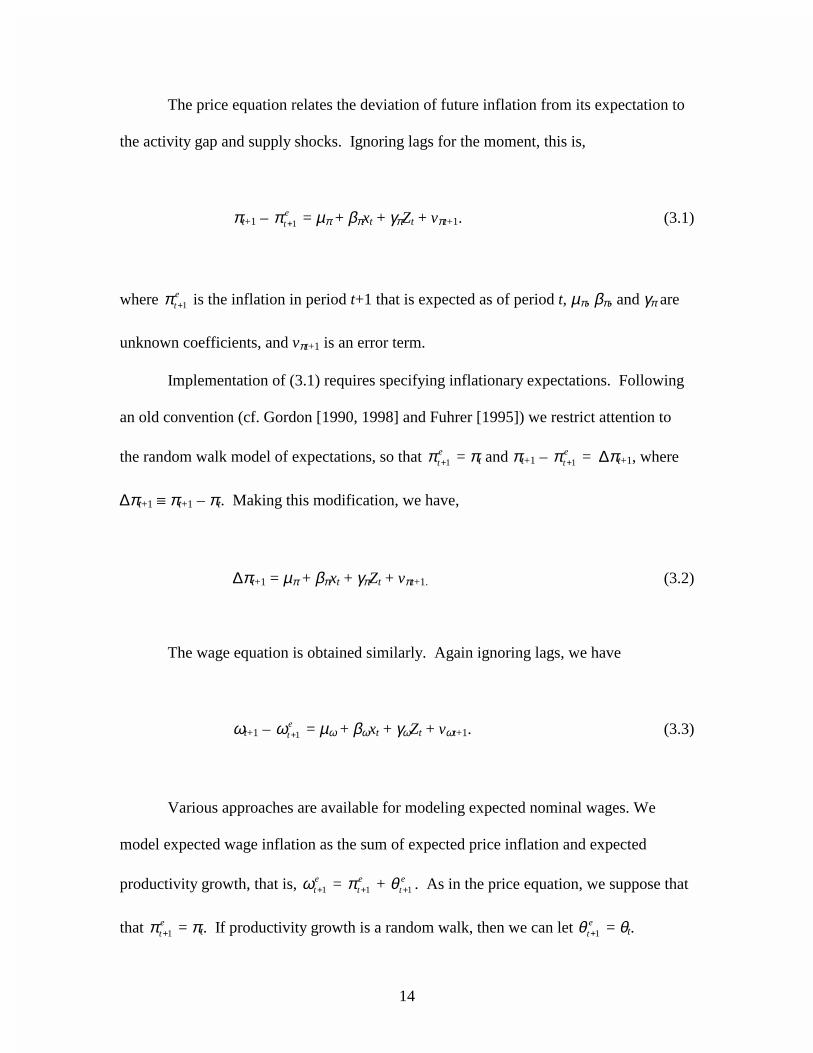
The price equation relates the deviation of future inflation from its expectation to

the activity gap and supply shocks. Ignoring lags for the moment, this is,

πt+1 – 1etπ + = µπ + βπxt + γπZt + vπt+1. (3.1)

where 1etπ + is the inflation in period t+1 that is expected as of period t, µπ, βπ, and γπ are

unknown coefficients, and vπt+1 is an error term.

Implementation of (3.1) requires specifying inflationary expectations. Following

an old convention (cf. Gordon [1990, 1998] and Fuhrer [1995]) we restrict attention to

the random walk model of expectations, so that 1etπ + = πt and πt+1 – 1

etπ + = ∆πt+1, where

∆πt+1 � πt+1 – πt. Making this modification, we have,

∆πt+1 = µπ + βπxt + γπZt + vπt+1. (3.2)

The wage equation is obtained similarly. Again ignoring lags, we have

ωt+1 – 1etω + = µω + βωxt + γωZt + vωt+1. (3.3)

Various approaches are available for modeling expected nominal wages. We

model expected wage inflation as the sum of expected price inflation and expected

productivity growth, that is, 1etω + = 1

etπ + + 1

etθ + . As in the price equation, we suppose that

that 1etπ + = πt. If productivity growth is a random walk, then we can let 1

etθ + = θt.

15

However, productivity growth has a cyclical component, so an alternative method used

by Gordon (1998) is to model 1etθ + = *

tθ , where *tθ is trend productivity growth. We will

use this latter approach as the base specification, but will also report results based on the

alternative specification in which 1etθ + = θt. This leads to a specification of the wage

equation of,

ωt+1–*tθ –πt = µω + βωxt + γωZt + vωt+1, (3.4)

Incorporation to lag dynamics. The specifications (3.2) and (3.4) omit lag

dynamics. Our treatment of dynamics is motivated by the observation, made in section

2.3, that nominal wage growth less productivity growth, or less trend productivity

growth, appears to be cointegrated with price inflation. That is, ωt+1–*tθ and πt are

arguably cointegrated. This leads to the triangular representation of cointegrated

variables, in which xt and Zt are treated as exogenous variables:

∆πt+1 = µπ + αππ(L)∆πt + απω(L)(ωt–*

1tθ − –πt-1) + βπxt + απx(L)∆xt + γπZt + vπt+1, (3.5)

ωt+1–*tθ –πt = µω + αωπ(L)∆πt + αωω(L)(ωt–

*1tθ − –πt-1) + βωxt + αωx(L)∆xt + γωZt + vωt+1.

(3.6)

where µπ, βπ, etc. are coefficients and αππ(L), etc. are lag polynomials. Specifications

(3.5) and (3.6) allow lagged effects of xt but, following the literature, not of the supply

shock variable Zt.

16

These two specifications form the basis for our time series analysis. The price

equation differs from most Phillips curve specifications because it includes a term

allowing feedback from real wages net of productivity to future price changes. The wage

equation also allows for feedback from price changes to future wage changes. Our

motivation for these equations has been to move from the static system (3.2) and (3.4)

using the tools of cointegration theory. Note however that our resulting equations are the

same as the general specification considered by Gordon (1998, equations (7) and (8)).2

An alternative specification that we explore in the empirical section adds a lag of

the level of productivity adjusted real wages (ln(Wt-1/Pt-1)-ln(Productivityt-1)) to the right

hand side of (2.5) and (2.6). This specification, a version of which goes back to the

classic paper by Sargan (1964), is appropriate when this term is I(0). As the analysis in

the last section suggested, this assumption seems at odds with the data used here, but

versions of the specification has been used for both wage and price equations using data

from the U.S. and other countries (c.f. Barlow and Stadler (undated), Blanchflower and

Oswald (1994), Brayton, Roberts and Williams (1999), and Holden and Nymoen

(1999).) Blanchard and Katz (1997) (and references cited there) contain a useful of

discussion of this specification as it applied to the wage Phillips curve, and we will

discuss this issue more in the context of the state Phillips curves specified in section 6.

3.2 Estimation of TV-NAIRUs

Specifications (3.5) and (3.6) use the “gap” variable xt, constructed as difference

between the activity variable and its univariate trend, but what should appear in the

2 Gordon’s (1998) derivation differs from ours, and he does not discuss cointegration explicitly. However, by imposing sums of coefficients in his lag polynomials to equal one (which he does in his empirical work),

17

Phillips curve is the deviation between the variable and the NAIRU. So, if the univariate

trend and the variable’s NAIRU are different, then (3.5) and (3.6) should include another

term that captures this difference. We model the difference between the NAIRU and the

univariate trend as a time varying intercept in these Phillips curves, and estimate this

difference from estimates of the time varying intercept.

To make this clear, consider the system in which the activity measure is the rate

of unemployment, ut, and let Ntu denote the possibly time-varying NAIRU. If the

NAIRU does not equal the univariate trend *tu , then (3.5) is properly specified as

∆πt+1 = µπ + αππ(L)∆πt + απω(L)(ωt-*

1tθ − -πt-1) + βπ(ut-Ntu ) + απu(L)∆(ut-

Ntu ) + γπZt + vπt+1

≅ (µπ+ βπ[ *tu - N

tu ])+ αππ(L)∆πt + απω(L)(ωt-*

1tθ − -πt-1) + βπgtu + απu(L)∆ut + γπZt + vπt+1

(3.7)

where gtu = ut -

*tu is the unemployment gap where second equation makes the

approximation that, because Ntu is slowly varying, the term απu(L)∆ N

tu is negligible.

Thus, to the extent that the univariate trend in unemployment *tu differs from the NAIRU

Ntu , the gap specification (3.5) will have a time varying intercept. An identical argument

applies to the wage equation (3.6).

This reasoning leads to a modification of the system (3.5) and (3.6), in which the

intercepts are allowed to vary over time:

the resulting system is equivalent to (3.2) and (3.4) which in turn implies that the system is cointegrated.

18

∆πt+1 = µπt + αππ(L)∆πt + απω(L)(ωt–*

1tθ − –πt-1) + βπgtu + απx(L)∆xt + γπZt + vπt+1, (3.8)

ωt+1–*tθ –πt = µωt + αωπ(L)∆πt + αωω(L)(ωt–

*1tθ − –πt-1) + βω

gtu + αωx(L)∆xt + γωZt + vωt+1.

(3.9)

If the slope coefficients are stable, any intercept drift in these equations arises from a

departure of the NAIRU from the trend unemployment rate.

Our method for estimating the intercept drift follows King, Stock and Watson

(1995), Staiger, Stock and Watson (1997b), and Gordon (1998) and adopts an unobserved

components model for the intercept, in which the intercept follows a random walk:

µπt+1 = µπt + ηπt+1, where ηπt+1 is i.i.d. N(0, 2

πησ ) (3.10)

µωt+1 = µωt + ηωt+1, where ηωt+1 is i.i.d. N(0, 2

ωησ ) (3.11)

The random walk specification is flexible way to track smooth changes in the intercept.

The initial condition for the random walk is identified by the unconditional means of the

regressors, so we construct the regressors to have mean zero and initialize the random

walk around zero.

According to the system (3.8) and (3.9), time variation in the wage and price

equation intercepts arises from changes in *tu - N

tu , and this means that the innovations

ηπt+1 and ηωt+1 should be the same. We shall examine this by estimating the intercept

drift separately for the price and wage equations and comparing the results. In addition,

we shall (separately) test the hypotheses that 2

πησ = 0 and 2

ωησ = 0 using the QLR or sup-

19

Wald test (Quandt [1960], Andrews [1993]). The parameters 2

πησ can be estimated by

maximum likelihood, but the MLE has a distribution that piles up at zero when these are

small and is thus unsatisfactory. Instead we construct confidence intervals and median-

unbiased estimates of 2

πησ and 2

ωησ using the methods in Stock and Watson (1998), as

discussed in Staiger, Stock and Watson (1997b) and Stock (1998, 1999).

The estimate of the NAIRU, ˆNtu based on one of these estimated equations is

obtained by combining the univariate drift and the intercept drift. Because µπt = βπ( *tu -

Ntu ) (with mean zero regressors), we have the estimator,

|*| ˆ

t TNt T tu u π

π

µβ

= − , (3.12)

where β̂ is the estimator of β and µπt|T is the estimator of µπt obtained from the Kalman

smoother based on the estimated parameters of the system.

We have motivated this treatment of the parameter drift by observing that we

want a consistent framework that is flexible enough to handle activity measures with

quite different trends. However, this formulation has two additional advantages. First, it

allows separate identification of the univariate trend and the NAIRU. Second, since

much of the time variation in the NAIRU is likely to be associated with changes in the

trend unemployment rate, the method can be viewed as a device akin to prewhitening to

obtain more precise estimates of the TV-NAIRU.

20

4. Macro Estimates of Price Phillips Curves

4.1 Benchmark Price Regressions

Benchmark estimates of regressions of the form (3.8), using various activity gaps,

are reported in table 2. The specifications include standard supply shock variables

(Gordon’s [1982] series for wage and price controls and the relative price of food and

energy). For comparability to conventional specifications, these specifications do not

include the error correction term (real wages less trend productivity, ωt-*

1tθ − -πt-1) or its

lags as regressors; these are included in results reported in the next section. The first row

reports the estimated value of the coefficient on the level of the activity gap (which is

equivalent to the sum of the coefficients on the current and lagged gaps in a specification

in which lags of xt, rather than of ∆xt), its standard error, and the p-value for the sup-Wald

statistic testing the stability of this coefficient. The second block of entries report the

trend value of the activity measure, and the third block of entries reports the estimated

TV-NAIRU (the sum of the univariate trend and the estimated deviation of the trend

arising from intercept drift). Standard errors for the NAIRU, and for its change since

1992, are computed using the Kalman smoother standard error formula and do not

incorporate estimation error, which would increase them. The final row reports the

median unbiased estimate of the standard deviation of the change in the intercept; if the

population counterpart of this coefficient is zero, there is no parameter drift, so the TV-

NAIRU for that activity measure equals its univariate trend.

Four results are notable. First, the slope coefficient shows the pro-cyclical nature

of the change in inflation and is statistically significant in each of these specifications.

21

The estimated value of the slope coefficient in the unemployment specification is

comparable to estimates obtained elsewhere in this literature using different sample

periods and different series, cf. Staiger, Stock and Watson (1997b, table 1) although they

are approximately half the size of the coefficients in Gordon (1998, table 3).

Second, the TV-NAIRU is estimated to have fallen by approximately 1.6

percentage points from 1992 to 2000; the decline is only slightly less if it is measured

using the demographically adjusted unemployment rate. In contrast, the NAIRU for

capacity utilization and building permits is relatively stable, for example, the decline in

the capacity utilization TV-NAIRU is only two-thirds of the Kalman smoother standard

error of the estimated decline.3

Third, for all practical purposes the estimated NAIRUs are simply the univariate

trends in the various activity measures. This can be seen by comparing the selected

univariate trend values and the estimated TV-NAIRUs shown in table 2, or the sample

paths of these values for the unemployment specification plotted in figure 3. The reason

why the TV-NAIRU and trend values are so similar follows from the data analysis in

Section 2. Neglecting lags and the supply shocks, the Phillips curve is

*1 1( ) ( )g N

t t t t tu u u vπ π ππ β β+ +∆ = − − + (4.1)

From the data analysis in section 2, ∆πt+1 is I(0), and by construction so is the

unemployment gap, gtu . This means that there cannot be large persistent deviations of

3 Garner (1994) pointed out the stability of Phillips curves specified with capacity utilization estimated with data through the early 1990s. Gordon (1998) and Stock (1998) estimated TV-NAIRUs for capacity

22

Ntu from *

tu : if there were, these would be transmitted to ∆π, but since ∆π is I(0), it does

not contain large persistent movements. Mechanically, this means that in all the

specifications, the median-unbiased estimate of the standard deviation of the intercept

drift is very small; indeed, it is nearly the same value in each specification, between 0.022

and 0.027. This corresponds to a change in the intercept between .044 and .054

percentage points per year, which is nearly two orders of magnitude less than the

standard deviation of the dependent variable, the quarterly change in inflation at an

annual rate. In all the specifications, the 90% confidence interval includes 0, so the

hypothesis of no parameter drift in these equations cannot be rejected at the 5%

significance level.

While the TV-NAIRU and univariate are very similar, figure 3 does show some

differences between Ntu and *

tu . The deviation in the 1960s and early 1970s is associated

with the trend increase in inflation over this period, and the deviation in the early 1980s is

associated with a decline in the trend rate of inflation.

The fourth result from table 2 concerns the time variation in the slope of the

Phillips curve. The p-values for tests of no slope change range from 0.02 to 0.16,

suggesting possible time variation in the slope. To investigate the magnitude and timing

of this variation, we estimated a model that allowed to slope coefficient to vary, but held

the intercept constant. Specifically, βπ was modeled as a random walk with innovation

variance estimated using the method described in Stock and Watson (1998). Figure 4

shows the estimates of the time varying slope coefficients for the specification using the

unemployment rate obtained by the Kalman smoother together with ±2 standard error

utilization and found they were quite stable compared with TV-NAIRUs for the unemployment rate. Our

23

bands and the OLS slope estimate. Most of the time variation evident in the slope occurs

in the mid 1970’s, and the estimated slope remained essentially unchanged during the

1990’s. Similar results obtain using the other variables (capacity utilization, building

permits and the demographically adjusted unemployment rate). These results are

consistent with some small amount of time variation in the Phillips curves slope over the

sample, but little time variation in the past dozen or so years.

4.2 Sensitivity Analysis

Table 3 summarizes 36 alternative Phillips curves regressions that examine the

sensitivity of the benchmark results in table 2. These regressions differ by: the price

index used to measure inflation; the activity measure used; whether supply shock control

variables are included; whether the error correction term and its lags are included;

whether the log-level of the productivity adjusted real wage (the “markup”) is included;

and how many lags are included in the specifications. The statistics reported in the table

are the same as in table 2, except that to save space the values of the level of the trend

activity measure and the associated TV-NAIRU are not reported; rather only the change

in the TV-NAIRU from 1992 to 2000 (and its Kalman smoother standard error, ignoring

estimation uncertainty) is reported.

These results suggest eight conclusions.

First, the specifications in which the unemployment rate gap is the activity

variable are robust to these changes. The coefficient on the unemployment rate gap is

fairly stable, with estimates ranging from -.25 to -.37 across specifications, with all the

estimated coefficients within a standard error of –0.3. The TV-NAIRUs estimated with

results confirm these findings and extend them through the end of the 1990s.

24

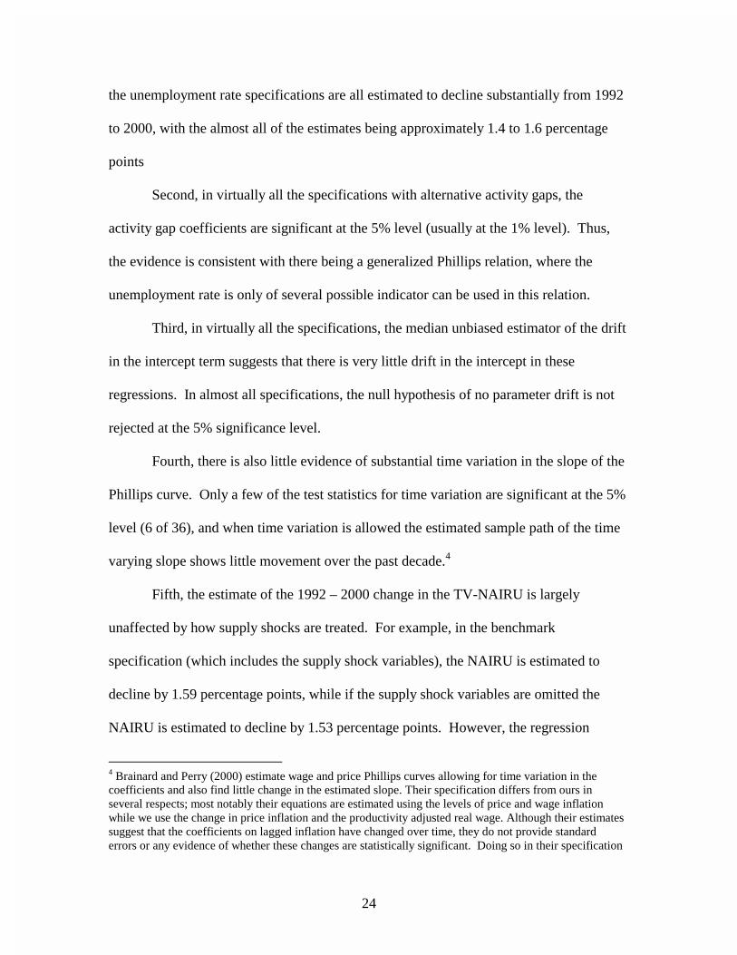
the unemployment rate specifications are all estimated to decline substantially from 1992

to 2000, with the almost all of the estimates being approximately 1.4 to 1.6 percentage

points

Second, in virtually all the specifications with alternative activity gaps, the

activity gap coefficients are significant at the 5% level (usually at the 1% level). Thus,

the evidence is consistent with there being a generalized Phillips relation, where the

unemployment rate is only of several possible indicator can be used in this relation.

Third, in virtually all the specifications, the median unbiased estimator of the drift

in the intercept term suggests that there is very little drift in the intercept in these

regressions. In almost all specifications, the null hypothesis of no parameter drift is not

rejected at the 5% significance level.

Fourth, there is also little evidence of substantial time variation in the slope of the

Phillips curve. Only a few of the test statistics for time variation are significant at the 5%

level (6 of 36), and when time variation is allowed the estimated sample path of the time

varying slope shows little movement over the past decade.4

Fifth, the estimate of the 1992 – 2000 change in the TV-NAIRU is largely

unaffected by how supply shocks are treated. For example, in the benchmark

specification (which includes the supply shock variables), the NAIRU is estimated to

decline by 1.59 percentage points, while if the supply shock variables are omitted the

NAIRU is estimated to decline by 1.53 percentage points. However, the regression

4 Brainard and Perry (2000) estimate wage and price Phillips curves allowing for time variation in the coefficients and also find little change in the estimated slope. Their specification differs from ours in several respects; most notably their equations are estimated using the levels of price and wage inflation while we use the change in price inflation and the productivity adjusted real wage. Although their estimates suggest that the coefficients on lagged inflation have changed over time, they do not provide standard errors or any evidence of whether these changes are statistically significant. Doing so in their specification

25

standard errors of the specifications with supply shocks are significantly smaller than

those with the supply shock omitted. Evidently these variables are important for

explaining one-off changes in inflation, but not the kind of persistent changes that could

be confused with a change in the NAIRU.

Sixth, the estimated recent decline in the TV-NAIRU is essentially unaffected by

whether the total unemployment rate or the demographically adjusted unemployment rate

is used. This is consistent with the discussion in Gordon (1998) and Stock (1999) that

although demographic shifts might be associated with increases in the NAIRU in the

1970s, the timing of demographic shifts is not aligned with this sharp recent decline.

Seventh, these results confirm the finding in table 2, columns (3) and (4) that TV-

NAIRUs estimated using the rate of capacity utilization and building permits have been

relatively stable; for capacity utilization the change from 1992 to 2000 is less than its

Kalman smoother standard error.

Eighth, adding the error correction term to the benchmark specification decreases

the standard error of the regression slightly but does not change the estimates of the slope

coefficient of the TV-NAIRU. This suggests that the estimated decline in the NAIRU is

not a spurious consequence of neglecting feedback from wages to prices. Table 3 also

shows results for a specification that includes the markup of prices over productivity

adjusted wages is included (or equivalently, when we include the log level of the

productivity adjusted real wage). Including this variable reduces somewhat the estimated

decline of the unemployment NAIRU, from 1.59 percentage points in the base

specification to 1.42 in the specification including this term. Thus, this term is estimated

would require handling the persistence of their regressors, in addition to the usual issues arising in time-varying coefficients.

26

to contribute perhaps 0.2 percentage points to the decline in the NAIRU. Taken together,

these results suggest that there is limited or no evidence that feedback from wages to

prices has particularly served to hold down prices during the 1990s.

4.3 Summary of Main Findings

The regression results in tables 2 and 3 indicate a stable and statistically

significant relation between future changes in price inflation and current economic

activity as measured by various activity gaps. In addition, in these gap specifications

there is very little evidence of drift in the intercept or the slope, either in terms of

statistical significance or in terms of the point estimates of the drift from 1992 to 2000.

Finally, including supply shocks does not change substantially the estimates of the

declines in the NAIRU.

We interpret these findings as being inconsistent with the “Phillips curve is dead”

theories of the 1990s. They are inconsistent with theories that place considerable weight

on changes in price setting behavior in the 1990s, for these theories would imply

important drift in the intercept or slope of the Phillips curve. They also are inconsistent

with theories that place great weight on sustained “good luck” in the form of favorable

supply shocks. Said differently, once the Phillips curves are specified in gaps, there are

no price equation puzzles to explain. Because trend capacity utilization and trend

building permits are approximately flat, the only “puzzle” about the price Phillips curve

is why the univariate trend in the unemployment rate has fallen. Once we have accounted

for the univariate trend in the unemployment rate, these price inflation Phillips curves fit

quite nicely throughout the decade and indeed throughout the 1960 –2000 sample period.

27

5. Macro Estimates of Wage Phillips Curves

This section presents empirical estimates of wage Phillips curves and TV-

NAIRUs using the unemployment rate and other indicators of economic activity. The

discussion parallels the previous section: section 5.1 presents some benchmark estimates;

the robustness of these estimates to alternative specifications are examined in section 5.2;

and conclusions are summarized in section 5.3.

5.1 Benchmark Wage Regressions

Benchmark regression estimates. Benchmark wage regressions are reported in

table 4, using the same format as table 2.

The most striking result in table 4 is that these specifications are very similar to

the benchmark price regressions reported in the corresponding columns of table 2. The

slope coefficients in table 4 are larger, but the standard deviation of the dependent

variable in table 4 is also larger than in table 2. The slope coefficients are all statistically

significant at the 5% level. Although the levels of the TV-NAIRUs are different in table

2 than in table 4 (because the variables have different means), the changes in the TV-

NAIRUs are almost the same.5 For example, the TV-NAIRU based on total

unemployment in the price equation in column 1 of table 2 is estimated to decline by 1.59

5 The difference between the levels of the NAIRUs in price and wage Phillips curve reflects the decline in labor’s share over the sample period computed using Nonfarm business (NFB) wages, NFB productivity and the GDP price deflator. This magnitude of this decline is evident from the 10th row of table 1. However, as the last row table 1 shows, there is a much smaller decline when the NFB price deflator is used. Consequently the levels of the NAIRU for the wage Phillips curves using the NFB deflator are closer to the values in the price Phillips curves.

28

percentage points from 1992 to 2000; based on the labor share specification in table 4,

this decline is estimated to be 1.52 percentage points. The quantitative declines in the

TV-NAIRUs are the same for the other activity variables in the two tables.

A key similarity between the price results in table 1 and the wage results in table 4

is that the intercept drift is negligible in both tables. Although the median unbiased

estimate is larger in table 4 than in table 2, the dependent variable in table 4 is more

variable and the standard error of the regression in the wage regressions is twice that of

the price regressions, so the relative variability in the intercept is virtually identical in the

price and wage specifications. In all specifications in table 4, the 90% confidence

interval for the standard deviation of the change in the intercept includes zero, that is, the

hypothesis of no parameter drift cannot be rejected in any of these specifications at the

5% significance level.

Figure 5 plots the estimated TV-NAIRU for unemployment based on the

specification in column 1 of table 4, where the TV-NAIRU is adjusted so that it has the

sample sample mean as the univariate trend in the unemployment rate (cf. footnote 5).

Inspection of this figure underscores that there is effectively no difference between the

TV-NAIRU and the univariate trend in unemployment. This is the same conclusion as

was drawn from the price TV-NAIRU plotted in figure 3. Comparison of figures 3 and 5

reveals that the TV-NAIRUs estimated from the price Phillips curve in table 2, column 1

and the wage Phillips curve in table 4, column 1 (shifted up per footnote 5) are essentially

identical. The reason for this is that, in both specifications, the median unbiased estimate

indicates negligible intercept drift.

29

Table 4 indicates that there is little evidence of changes in the slope of the wage

Phillips curve. The p-values for the test of the null hypothesis of no change in the slope

ranges from 0.10 to 0.99. Figure 6 shows the estimated values of the time varying slope

in the unemployment rate wage Phillips curve using a specification that parallels the

results for the price Phillips curve shown in figure 4. The point estimates suggest a slight

steepening of the wage Phillips curve over the past decade (consistent with the scatterplot

in figure 1b), but the standard error bands make it clear that these changes are far from

statistically significant.

5.2 Sensitivity Analysis

Table 5 summarizes results for 48 variations of the wage Phillips curves. Some of

these variations are similar to the sensitivity checks reported in table 3, for example

changing the definition of the wage series, changing the number of lags, etc. Inspection

of table 5 reveals that main conclusions from table 4, particularly the lack of intercept and

slope drift in the gap specifications, are robust to these changes. However, there are

some important differences among these specifications.

Most notably, these wage specifications are less stable than the price

specifications to changes in definitions of the variables. For example, the slope

coefficient is often insignificant in specifications in which the GDP deflator is replaced

by the PCE deflator or the CPI, as well as in specifications in which wage growth is

measured using the ECI (total compensation or wages and salaries) or average hourly

earnings. (The sample period for the specifications using the ECI data was limited to

1982-1999.) The results using compensation per hour are, however, consistent with the

30

benchmark results. Overall, however, these results suggest that the presence of a Phillips

curve specified using trend unit labor costs are rather delicate.

An important result in table 5 is that replacing trend productivity growth with its

sample average growth rate results in coefficients on the activity variable that are

essentially unchanged, but induces intercept drift that is both economically large and,

now, statistically significant. In contrast to the benchmark estimate, in which the

unemployment rate TV-NAIRU is estimated to have fallen by 1.52 percent from 1992 –

2000, the specification using average productivity growth shows a decline of only 0.79

percentage points in the estimated TV-NAIRU. Said differently, when the recent

increase in trend productivity is excluded from the specification, the intercept in Phillips

curve adjusts to track the increase in real wages. The amount of the required adjustment

is large: the change in the intercept implies an increase in the long run mean change in

the growth rate of wages by 0.84 percentage points.

5.3 Summary of Main Findings

These regressions point to a stable Phillips relation between trend unit labor costs

and the various activity measures over this period, although the macro wage

specifications are more delicate than the macro price specifications examined in section

4. When the slope coefficient is precisely estimated, these specifications produce

estimates of the 1992 – 2000 change in the TV-NAIRU that are strikingly similar to those

produced by the price Phillips curves. In contrast, if the dependent variable is future

wage inflation less current price inflation, so that the role of productivity growth is

ignored, then the behavior of the wage and price regressions is inconsistent, with real

31

wage inflation appearing in the second half of the 1990s. Specifications of the wage

Phillips curves that ignore productivity growth appear unstable in the 1990s, while

specifications that incorporate the productivity growth are stable.

6. Specification and Estimation of State Wage Phillips Curves

6.1 Specification of State-Level Wage Phillips Curves

The state regression specifications have the same basic form as the macro

regressions, but data limitations lead to several modifications. For example, because the

state data are annual, the timing conventions of the quarterly and annual specifications

differ. Temporal aggregation by averaging both sides of (3.4) over the four quarters in

the year results in a relation between time series with dates that overlap by three quarters.

We approximate this by using as the dependent variable ωt+1-θt+1-πt+1 (robustness to

different timing conventions is investigated in section 8.2). Also, we use the

unemployment rate as the activity variable in all of the state Phillips curves.

These considerations lead to the state-level variant of (3.4),

ωit+1–θit+1–πt+1 = β(uit – Nitu ) + ζt + vit+1, (6.1)

where ωit+1 is the percentage growth in the nominal wage in state i from year t to year

t+1, θit+1 is the annual percentage growth in labor productivity, uit is the unemployment

rate, Nitu is the NAIRU for state i in year t (i.e. the state TV-NAIRU) , ζt are macro

shocks (the sum of γωZt and vt+1 in (3.4)), and vit is an error term that has mean zero and

32

which is uncorrelated with the macro shocks ζt. The subscript t runs over the years in the

sample, which differ slightly across specifications depending on data availability. As is

discussed in the next section, in our data set state nominal wage growth ωit+1 and the

unemployment rate uit are computed from the Current Population Survey (CPS). State

productivity θit is constructed in two different ways, either as the annual percentage

growth of gross state product, less the growth of state employment, or from national

industry-level productivity data weighted by the output share of each industry in the state.

The state TV-NAIRU can usefully be thought of as consisting of several

components: the national TV-NAIRU ( Ntu ), features that are unique to each state which

are constant over the sample such as climate (φi), and institutional considerations that

affect search and matching in the labor market, some of which are measured (Xit) and

some of which are not (εit). That is, the state TV-NAIRU can be expressed as,

N Nit t i it itu u Xφ γ ε= + + +� . (6.2)

Substitution of (6.2) into (6.1) and rearranging yields our base state regression

specification:

ωit+1–θit+1–πt+1 = αi + δt + βuit + γXit + vit+1, (6.3)

where αi = –βφi are state effects and δt = ζt – β Ntu are time effects.

33

It is worth making three remarks about the specification (6.3). First, unlike the

macro regressions, this benchmark specification for the state panel regressions does not

include lags of either the unemployment rate or the labor share. The reason for this is

practical: with only twenty annual observations, it is unlikely that we will estimate lag

dynamics with any precision, and in any event the lag dynamics will be less pronounced

at the annual level than at the quarterly level used in the macro data. In sensitivity

checks, however, we report the results of specifications that include lags.

Second, as we discussed above, there is some debate over whether the correct

specification of this model should include a lagged wage level on the right hand side –

i.e. should the model be specified in terms of wage levels (the “wage curve”) or real wage

growth less productivity (the Phillips curve)? Specifications using wage growth have the

implication that states’ productivity-adjusted real wages can drift arbitrarily far apart over

long periods, and this is implausible since capital and labor can flow across state

boundaries. However, the empirical evidence suggests that capital and labor migrate

slowly enough that the Phillips curve specification fits that data better than wage curve

specifications with substantial mean reversion (cf., Blanchard and Katz (1992, 1997),

Card and Hyslop (1997), Autor and Staiger (in progress)). This leads us to use the

Phillips curve as our benchmark specification, although in our sensitivity analysis we

consider specifications that include the levels of productivity adjusted real wages.

Third, πt is not indexed by state in (6.3). This is done because data on prices by

state are not available; thus, deflation is done using the national price level (the CPI-U).

Because (6.3) includes state effects, this means that the estimates of the slope coefficients

β and γ are invariant to which inflation variable is used (CPI, GDP deflator, etc.), whether

34

it is dated t+1 or t, or indeed whether the dependent variable is not deflated at all (i.e. is

ωit+1–θit+1). The only role of the deflator is to identify the time effects {δt} and thereby to

identify the macro TV-NAIRU from this state specification.

6.2 Estimation of a National TV-NAIRU from the State Regressions

Estimates of the annual national TV-NAIRU can be obtained from the year effects

in the state regressions. The year fixed effects contain movements in the national TV-

NAIRU, macro shocks, and estimation error. Thus, these year fixed effects must be

filtered to obtain estimates of the national TV-NAIRU.

The filtering strategy used here parallels that used in the macro analysis. That is,

the filter is applied so that it estimates the difference between the TV-NAIRU and the

univariate trend in unemployment; this univariate trend is then added back in to obtain

an estimate of the national TV-NAIRU. Specifically, as noted following (6.3), δt = ζt –

β Ntu . To maintain consistency with the treatment of the NAIRU in the macro

regressions, rewrite this as, δt + β *tu = ζt – β( N

tu – *tu ), where *

tu is the univariate trend in

unemployment. Thus,

δt + β *tu = µt + ζt, (6.4)

where µt = – β( Ntu – *

tu ).

Equation (6.4) has the same form as (3.9), in the sense that the intercept drift term

µt arises from the difference between the NAIRU and the univariate trend in

35

unemployment, except that (6.4) has no regressors (the observable and unobservable

macro shocks are combined and contained in ζt). Accordingly, the national TV-NAIRU

is estimated as |Nt Tu = *

tu + µt|T/ β̂ (see equation (3.12), where β̂ is the estimate of β from

the state regressions and µt|T is the Kalman smoother estimate of µt, where µt is modeled

as following a random walk (as in equation (3.10)), ζt is modeled as serially uncorrelated,

and the dependent variable in (6.4) is *ˆ ˆt tuδ β+ , where t̂δ are the estimated time effects.

6.3 Instrumental Variables Estimation Strategy

As is discussed in the next section, the state data on unemployment are obtained

from the merged outgoing rotation groups (MORG) of the Current Population Survey

(CPS). Because many states have a small number of CPS respondents, these estimates

are quite noisy, which leads to errors-in-variables bias. To avoid this bias, we use an IV

approach. The MORG sample can be split into two independent samples, depending on

whether the month is odd or even (although households appear twice in the MORG, the

odd and even months have no households in common). Estimates from both the odd and

even month samples will be measured with error, but because the samples are randomly

drawn the estimation error is independent in these two samples. Thus one set of

estimates can be used as an instrument for the other set of estimates. In particular, we use

unemployment rates estimated from the even months as in instrument for unemployment

rates estimated in the odd months, and vice versa. In some of our specification (e.g. those

with lags of the dependent variable) the measurement error will be correlated between the

independent and dependent variables as well. Therefore, we replace all variables in the

36

equation (both dependent and independent) with estimates from odd months, and

instrument with corresponding estimates from even months.6

6.4 Weighting the Observations

There is some ambiguity about whether the state regressions are best estimated by

weighting the observations. The sampling error in the dependent variable will be smaller

for larger states, but this sampling error is only one component of the error term, so the

actual form of heteroskedasticity is unknown. Simple IV (2SLS) has the virtue of taking

no stand on the form of this heteroskedasticity, and treats each state as an independent,

equally useful experiment. On the other hand, weighting the observations can provide an

approximate adjustment for this heteroskedasticity, and if implemented using

employment weights it also produces estimates more directly related to aggregate

coefficients, in particular the aggregate NAIRU estimates constructed from the state data

will reflect population weights. Because of this ambiguity, we report results using both

weighted and unweighted observations, where the weights are given the values of state

employment.

6 This instrumenting strategy is simple but statistically inefficient. For an alternative more efficient method see Autor and Staiger (in progress).

37

7. The State Data Set

Our state-level analysis relies on a dataset containing annual observations on each

of 48 states (excluding DC, Alaska and Hawaii) from 1979 to 1999. The annual data on

each state were derived from a variety of sources as described below.

7.1 Data Derived from the Current Population Survey

We derive most of our variables, including annual estimates of wages,

unemployment, and labor force characteristics for each state, from the merged outgoing

rotation groups (MORG) of the CPS. The MORG data are available from 1979 through

1999. One quarter of the CPS sample each month (the outgoing rotation groups) is asked

a variety of labor force questions, for a total sample of over 300,000 individuals each

year. For each individual who reports being in the labor force, the survey provides the

person’s labor force status (unemployed or not in reference week), gender, race

(white/black/other), gender, marital status (married or not) and age. Education is

reported in each year, but because the format of the question changed in 1992 we have

recoded the education variable into a set of 10 consistent categories. Most recent

industry of employment is reported by all individuals who have worked in the last 5

years, and we collapsed this information into 11 major industries.

For individuals who are currently working, we calculated their hourly wage as

usual weekly earnings divided by usual weekly hours. Earnings at the topcode were

multiplied by 1.5, and wages below the 1st percentile were set equal to the wage at the 1st

percentile. We also calculated whether these persons were self-employed, a union

38

member or covered by a union contract (only available since 1983) or worked as

temporary help. To be defined as a temporary help worker, one had to report working in

the Personnel Supply Services industry, and report being paid by the hour. This

definition is the same as that used by Autor (2001) and Segal and Sullivan (1997), but it

is believed that at least 50% of temporary workers misreport their industry in the CPS.

Finally, we calculated potential experience as age minus years of education minus 6,

where years of education were imputed after 1991 based on the respondent’s reported

education category, race and gender.

Using the individual-level data for all individuals who were in the labor force

from the MORG, we constructed state-level estimates for each year based on three

samples: the full MORG, the respondents from even-numbered months, and the

respondents from odd-numbered months. Households that appear in the MORG sample

in even-numbered months do not appear in the odd-numbered months, so as noted above,

that estimation error in these two samples will be independent. In each sample, we

constructed weighted estimates for each state and year (using weights provided by the

CPS) of the unemployment rate, and the fraction of the labor force in each age, education,

race, and gender category. In addition, for employed individuals we calculated the

fraction of the workforce in each major industry, working in the temporary help industry,

self-employed, and covered by a union contract (or a union member). Finally, we

calculated average and median log hourly wages for all workers, for hourly workers, and

for full-time workers.

To construct state-level estimates of wages and unemployment that adjusted for

changes over time in characteristics of the workforce, we estimated separate cross-section

39

regressions for each year. In particular, for each year we estimated a regression of either

unemployment status or the log hourly wage on state fixed effects and controlled for 10

education categories, 3 race categories, a quartic in experience, and an interaction

between gender and all other regressors. In addition, controls for 11 major industries

were included in the wage equation (but not the unemployment equation). Based on this

regression, each state’s adjusted mean wage was predicted using that state’s intercept and

the average value of the covariates in the US over 79-98 period (calculated from the

MORG).

7.2 Supplemental State Level Data

In addition to the MORG data, we use a variety of labor market measures that are

available by state and year over most of our time period.7 Data for each state on the UI

replacement rate are available through 1998 from the Information Technology Support

Center (ITSC) Unemployment Insurance web site (www.itsc.state.md.us). Data on the

minimum wage has been derived from various issues of the Monthly Labor Relations

Review. Data on the proportion of employment in the temporary services sector comes

from county business patterns (this data is only available through 1996, so our

specifications use it with a one year lag to avoid losing observations). Finally, the

proportion of the population age 25-64 on DI and SSI has been estimated from

administrative data and provided to us by David Autor and Mark Duggan.

State estimates of labor productivity growth were derived from data on Gross

State Product (GSP) and total full-time and part-time employment (from Table SA25)

available from the BEA web site by state and major industry for 1978-1998

40

(www.bea.doc.gov). For each state, we constructed estimates of labor productivity

growth in two ways. Our primary method uses state-level estimates of GSP and

employment, and calculates labor productivity growth in each year as 100[ln(GSPt/GSPt-

1) – ln(employmentt/employmentt-1)]. Our secondary method is to estimate productivity

growth in each state as a weighted average of the national-level estimates of labor

productivity growth in 11 major industries. National-level estimates of labor productivity

growth in each industry were derived from national estimates of GSP and employment as

above. Each industry’s productivity growth was weighted by the employment share in

that industry (as estimated from the MORG) in a given state and year to derive state-level

estimates of labor productivity growth.

8. Empirical Sate Wage Phillips Curves

8.1 Benchmark Estimated Phillips Curves

Benchmark wage Phillips curve regressions of the form (6.3) are reported in table

6. These benchmark regressions do not include any structural variables (Xit) that might

explain the movements in the NAIRU; these variables will be added in section 9.

Four features of table 6 are noteworthy. First, including state effects substantially

changes the value of the coefficient on the unemployment rate. Although the state effects

are usually jointly insignificant at the 5% level in these and subsequent regressions,

7 We thank David Autor for providing us with much of this data.

41

excluding them evidently introduces omitted variables bias into the estimated slope so

henceforth the state effects will be retained.

Second, using IV estimation to mitigate errors in variables bias leads to

coefficients on the unemployment rate that are approximately one-third larger than the

OLS estimates. This is consistent with the standard measurement error model and its

prediction that errors-in-variables biases the OLS estimate towards zero. An important

issue in IV regression is whether the instruments are correlated with the variable they are

instrumenting; that is, whether they are “weak” or not. When there is a single variable

being instrumented, this can be checked by seeing if the F-statistic on the instruments in

the first stage regression is at least 10 (Staiger and Stock [1997]). For the regressions in

table 6, this first stage F is always at least 100, which gives us confidence in applying

standard asymptotic distribution theory to these IV regressions.

Third, the time effects are jointly significant in all specifications.

Fourth, the estimated slope of the state Phillips curve is large and statistically

significant. In our preferred specification (IV with state and time effects), the estimated

slope is -.59 with a standard error of .11. This estimate is twice what we obtained using

the quarterly macro data (-.28 in table 2, column 1), although it is comparable to the

macro estimates in Gordon (1998). Because the state regressions control for both time

and state effects, these results suggest that idiosyncratic movements in a state’s

unemployment rate portend large idiosyncratic changes in the rate of growth of real

wages.

42

8.2 Sensitivity Analysis

Tables 7 and 8 summarize results from several modifications to the benchmark

specification. Table 7 shows results from changes in the estimation procedure (weighting

the observations and alternative IV estimators); changes in the wage and unemployment

variables (adjustments for changing demographics, industry mix, etc.); changes in the

measure and treatment of productivity; and changes in the assumed timing of the

variables. Table 8 summarizes results from specifications with more general dynamics.

We discuss each of these in turn.

The first two rows of table 7 consider different estimators. The benchmark

specification (IV with time and state effects, shown in the last column of table 6 and

repeated at the top of table 7), used unweighted observations with observations for even

months of the MORG used as instruments for observations corresponding to odd months.

Specification (1) in table 7 reverses this and uses odd months as instruments for the even

months. Specification (2) weights the state observations by state employment. In both

specifications, this results in little change from the benchmark model.

Specifications (3)-(9) use different measures of wages and the unemployment

rate. Specifications (3)-(6) use adjusted wage and employment data. The adjusted

measures were computed by controlling for education, experience, race, gender, and

industry (depending on the variable and specification) as detailed in the table notes, using

the adjustment method described in section 7.1. The benchmark specification uses the

sample average wages of all workers (as described in section 7.1) and specifications (7)-

(9) consider alternative wage series (median wage of all workers, mean wage of full time

43

workers, mean wage of hourly employees). The slope coefficient on the unemployment

rate is essentially unaffected by these modifications to the benchmark specification.

Specifications (10)-(12) modify the way productivity enters the model.

Specification (10) omits productivity from the analysis, so that the dependent variable in

the regression is the log of real wage growth. Specification (11) adds productivity as a

regressor, relaxing the constraint of a unit elasticity implicit in the benchmark model.

Both of these changes to the benchmark specification lead to slightly larger estimates of

the slope coefficient. The estimated productivity elasticity from specification (11) (not

shown) is small (0.17 with a standard error of .13). There are several possible

explanations for this. This result is consistent with substantial measurement error in the

state productivity data. Additionally, even state productivity, precisely measured,

contains short term fluctuations, and if it is trend productivity rather than annual

productivity that is reflected in wages (as we have assumed in the macro specifications)

then these estimates would be further biased towards zero. Finally, it might be that

productivity only affects wage growth with a lag, an explanation that we investigate

below.

Specification (12) uses an alternative measure of state productivity, the weighted

average industry productivity growth that was described in section 7.2. This change

produces a further steepening of the estimated Phillips curve.

The final two specifications in table 7 change the dating of productivity growth

and then unemployment rate. Specification (13) uses replaces θit+1 with θit, and

specification (14) replaces uit with uit+1. Both changes result in a somewhat smaller

44

estimated slope, suggesting that the timing convention in the benchmark specification is

appropriate.

Changes in the dynamic specification. Table 8 considers changes in the dynamic

specification of the model. Table 8a allows the lagged level of productivity adjusted real

wages to enter the regression, relaxing the unit root constraint implied by the Phillips

curve specification. We show results for both OLS and IV, specifications that include

and exclude the productivity adjustments to real wages, and specifications that include

the demographic and industry mix adjustments to wages. The OLS estimates show some

evidence supporting mean reversion in real wages: the coefficients on lagged real wages

range from -.09 to -.15 (implying AR roots of .85 to .91 for annual real wages) and

appear to be statistically significant. However, measurement error in the MORG wage

series imply that the OLS estimators have a negative bias. When IV is used to eliminate

this bias, the estimated coefficients on lagged wages are much closer to zero and are

statistically insignificant in the specifications that include productivity adjustments. (See

Blanchard and Katz (1997) for similar estimates.)

Table 8b summarizes results for two specifications that allow distributed lags of

wage growth and the unemployment rate in the model. These changes have little effect

on the estimated slope of the Phillips curve, and the additional lagged variables are

jointly insignificant in the regression.

Summary of the sensitivity analysis. The benchmark specification relates annual

observations of productivity adjusted real wage growth to unemployment rates one year

earlier together with time and state effects. The estimated slope is approximately –0.6

45

and there are no additional dynamics. The results in tables 7 and 8 are broadly consistent

with this specification.

8.3 National TV-NAIRUs Estimated Using the State Data

Estimates of the national TV-NAIRU derived from the estimated time effects in

the benchmark model are plotted in figure 7. Also shown are results from the

specification that omits productivity and uses the real wage instead of unit labor cost as

the dependent variables (specification (10) of table 7). These estimates were computed

by the method described in section 6.2. The figure also plots the national unemployment

rate and its univariate trend. The mean of the dependent variables in the two state

regressions differ, so for comparison purposes the state estimates of the national TV-

NAIRUs have been shifted so that they have the same mean as the national

unemployment rate over the 1979-1997 period.

The estimated national TV-NAIRU based on the state unit labor cost regression is

similar to the univariate trend in national unemployment, and thus is similar to the TV-

NAIRUs estimated using the macro data. In contrast, the estimated national TV-NAIRU

based on the state real wage regression falls only slightly in the 1990s. Mechanically,

this arises because the real wage regressions implicitly introduce drift in the mean

productivity growth rate into the NAIRU: the sharp increase in real wages in the late

1990s implies that the unemployment rate must have been well below the NAIRU during

this period, if one neglects increases in the growth rate of productivity. Upon

incorporating productivity into the dependent variable in the state panel regressions, the

NAIRU falls substantially. This, then, is consistent with the conclusion from the analysis

46

of the macro data that incorporating productivity reconciles the strong real wage growth

of the 1990s with an estimate of a declining unemployment TV-NAIRU estimated in

price regressions.

We conclude from these estimates that, despite substantial differences in the data

sets, span, and periodicity, the state and macro evidence are mutually consistent. This

sanguine conclusion must be tempered by a recognition that both the state estimates of

the TV-NAIRUs are quite imprecise: the Kalman smoother estimate of the standard error

on the decline in the state estimate of the TV-NAIRU from 1992 to 1997 using unit labor

costs is 0.7 percentage points, and this standard error ignores estimation error. This

imprecision should not be too surprising because the national estimates are based on

smoothing the time series of estimated time effects that has only 20 annual observations.

9. State Evidence on Structural Sources of Shifts in the NAIRU

This section reports the results of state panel regressions that examine the stability

of the Phillips curve over time and across regions and that include variables that represent

possible structural factors that determine the NAIRU. Our conclusions from the state

regressions are summarized at the end of this section.

9.1 Stability

The stability of the wage Phillips curves over time and across regions is

investigated in table 9. There is no evidence that the slope of the Phillips has changed

over time. This is shown in table 9 using productivity adjusted real wage growth; similar

47

results, not reported in the table, were obtained using real wage growth without a

productivity adjustment. This confirms Katz and Krueger’s (1999) results using OLS

that the state Phillips curve has been stable over time.

Interestingly, there is some evidence that the coefficient on the unemployment

rate differs depending on the region of the country (where regions are defined to be the

four Census regions). The Northeast and the West are estimated to have flatter Phillips

curves than elsewhere. These regional interactions are marginally significant (the p-value

is .07). Understanding whether there actually is regional variation in this slope, and if so

why, is an interesting topic for future resource.

9.2 Demographics and Education

We now turn to regressions that investigate possible structural reasons that the

NAIRU might change over time. The first such regressions examine the role of

demographics and education, a theme recently emphasized by Shimer (1998).

Table 10 reports the results of regressions which include, either individually or

together, the percent of high school dropouts, the percent of college graduates, the

percent white in the work force, the percent female in the workforce, and the percent of

the workforce aged between 25 and 54 years. These variables and the unemployment rate

are measured in percentage points. The estimated coefficients are large, but so are their

standard errors, and none of the demographic or education variables are statistically

significant at the 5% level, either individually or jointly. For example, the coefficient on

the percent of high school dropouts in the second column is –0.099, which implies that a

one percentage point increase in the fraction of high school dropouts is associated with a

48

decrease in the NAIRU of 0.15 percentage points (-.099/.642). However the standard

error of this estimated effect is very large (0.23 percentage points) so that this

specification produces a 95% confidence interval for the effect of a 1 percentage point

increase in high school dropouts on the NAIRU that ranges from a decline of 0.6

percentage points to an increase of 0.3 percentage points. The large standard errors

reflect the fact that, once state and time effects have been removed, there is only limited

within-state variation in these slow moving demographic variables.

Lerman and Schmidt (1999) have claimed that the recent rise (and impending

decline) in the share of prime-age workers, along with the continuing rise in the share of

college-educated workers, are key factors in understanding recent (and future) changes in

the labor market.8 However, the timing of these demographic shifts do not coincide well

with the downturn in the estimated NAIRU since 1992. In particular, the share of the

workforce with a college degree increased steadily in both the 1980s and 1990s, which

would suggest a steady decline in the NAIRU over the entire period. Similarly, the share

of the workforce between the ages of 25 and 54 increased dramatically between 1979 and

1992, but has been flat or even declined since then. Thus, neither of these factors

increased at a higher rate in the 90s, which is what would be needed to explain the sudden

decline in the NAIRU after 1992. Despite the inability of these demographic shifts to

explain recent changes in the NAIRU, it is worth noting that the point estimates imply

8 Lerman and Schmidt (1999) also present some limited evidence suggesting that there is no relationship between the unemployment rate and wage growth in the late 1990s, which is at odds with the evidence we present in table 6. In particular, they report no relationship between growth in wages at the state level from 1995 (Q1) to 1998 (Q1) and a state’s unemployment rate quartile in 1998 (Q1), based on three months of CPS data from 1995 and 1998. A number of aspects of the Lerman and Schmidt evidence are likely to bias their estimate toward finding no relationship. In particular, the small sample sizes from using only 3 months of data exacerbate the measurement error issues in the unemployment rate. More importantly, their focus on a single 3-year difference with unemployment measured at the end of the difference is at odds with the usual Phillips curve specification that focuses on short differences and lagged unemployment.

49

that the impending decline in the share of prime-age workers over the next twenty years

(as the baby boomers retire) would exert upward pressure on the NAIRU. Thus,

reconciling the state-level estimates of demographic effects on the NAIRU with the

macro-level evidence in changes in the NAIRU is an important topic of future research.

9.3 Industry Characteristics and Temporary Help

Table 11 reports results for regressions including industry characteristics and the

relative size of the temporary help industry in the state.

The results suggest that increases in the share of retail trade and services are

associated with increases in the NAIRU, relative to manufacturing, but these effects are

not statistically significant. Similarly, the point estimates suggest that increases in

temporary help and self employment lead to declines in the NAIRU, but again, these

estimated effects are not statistically significant.9

9.4 Government Policies

Table 12 examines the effect of state labor market policies on the NAIRU. These

include the percent of the prime aged workforce on social security disability or SSI, the

minimum wage, the growth of the minimum wage, and the unemployment insurance

replacement rate.

None of the coefficients on these regressors is statistically significant at the 5%

level in any of the specifications.

50

9.5 Summary of State Results

The finding that the unemployment rate significantly enters equations for either

the change in labor share or real wage equations is highly robust to changes in

specification, including lags, using different measures of wages, using demographically

adjusted data, and controlling for a large number of possible structural determinants of

the NAIRU. The coefficient is estimated to be approximately –0.6. This coefficient is

stable over time, although there seem to be some intriguing but uninvestigated variations

in this coefficient over different regions of the country.

In contrast, the state evidence on the determinants of the NAIRU is generally

negative. None of the state labor market policy variables enter statistically significantly.

Neither industry composition nor the size of the temporary help sector are statistically

significant determinants of the NAIRU in the IV regressions. Of the demographic and

education variables, there is some evidence that relatively more workers in the prime age

work group contribute to reductions in the NAIRU, but this effect is estimated very

imprecisely.

Despite the lack of statistical significance of these effects, it is worth checking

whether the point estimates of the coefficients are consistent with these variables

potentially having an economically substantial effect on the NAIRU, and in particular the

evolution of the NAIRU through the 1990s. The point estimates associated with the

demographic variables are, in fact, consistent with these variables having economically

large effects, but the timing of these effects is inconsistent with their playing an important

role in the fall in the NAIRU since 1992; rather, they contribute to a decline in the

9 Katz and Krueger (1999) find a statistically significant effect of temporary help on the NAIRU in Phillips curves estimated from state data. Their result appears to depend in an important way on the particulars of

51

NAIRU prior to 1992, but their contribution is estimated to have increased the national

NAIRU since 1992.

The point estimates associated with the industry mix variables, including

temporary help (table 11, last column) do point to a contribution that would lower the

NAIRU by approximately half a percentage point from 1992 to 1997, but this effect is not

statistically significant.

Overall, these state panel regressions fail to pinpoint any economic determinants

of the TV-NAIRU. This accords with the macro evidence in Stock (1999) that education

and demographic variables are inconsistent at the macro level with the trends in the

NAIRU. Our finding contrasts somewhat with Katz and Krueger, who find some

evidence that the rise of the temporary help industry has contributed to the fall in the

national NAIRU (they estimate that temporary help has reduced the national TV-NAIRU

by approximately 0.4 percentage points since 1990). Our specifications differ somewhat

from theirs, however, and we find that the effect of temporary help is not robust.

10. Conclusions

We assess these results by returning to the three questions of the introduction.

First did the Phillips curve break down in the 1990s, or did it simply shift, with a

new and evolving NAIRU? In both our macro and state analysis, we found abundant

evidence of a stable relation both between both the change in price inflation and activity

gaps of economic activity, and between unit labor costs and these activity gaps. These

their specification and estimator (OLS).

52

two pieces of evidence are confirmatory and are particularly striking because the state

panel estimates included time effects, thereby eliminating the variation in the data that

drives the macro estimates. Moreover, in the macro analysis we found evidence that

there was little intercept drift when the regressions were estimated as gaps; that is, when

specified in gaps, neither the price nor the wage Phillips curve has shifted in the 1990s.

Thus, this evidence falls squarely on the side of the “Phillips curve is alive and well

but...” theories.

Second, given this finding, why has the price Phillips curve shifted in? The

macro analysis suggests that the answer is not that we have had a particularly fortunate

string of supply shocks; we did in the mid-1990s, but they were subsequently reversed.

In addition, both the macro and state evidence suggests that an autonomous shift in wage

or price setting behavior by firms also is not an important part of the inflation-

unemployment story of the 1990s: had changes in price or wage setting behavior been the

reason for the apparent decline in the NAIRU, the NAIRU and the univariate trend in

unemployment would differ, but they do not. This finding is reinforced by the limited

role we found for industry mix variables in the state panel data analysis. This suggests

that labor market factors, such as demographics, the rise of the temporary help industry,

or labor market policies must be the source of the changes in the NAIRU. Curiously,

however, our results do not point in this direction. The macro estimates of the change in

the NAIRU from 1992 – 2000 using the demographically adjusted unemployment rate are

virtually the same as using the total unemployment rate. Similarly, our attempts to

identify structural determinants of the NAIRU using the state data were disappointing.

53

Several effects pointed in the right direction, but the state data did not provide precise

estimates of these effects.

Third, can the labor productivity gains of the 1990s explain the apparently

aberrant recent behavior of real wages in Figure 1b? Yes: the TV-NAIRUs estimated

both on the macro and state data are the same whether the change in inflation or real

wages less productivity are the dependent variable, and differ sharply during the 1990s

only when the productivity component is omitted from wages.

The simplest summary of these results is that, once one accounts for the univariate

trends in the unemployment rate and in productivity, the1990s present no price or wage

puzzles. Thus, the task is to explain trend movements in productivity and in

unemployment. In our framework, trend unemployment and the NAIRU are identified

separately, but as it happens these two series track each other very closely. Because the

long run trend components of the rates of inflation and unemployment are essentially

unrelated in the postwar U.S. data (Stock and Watson [1999a]), we are skeptical of

explanations that link the two such as those of Akerlof, Dickens and Perry (1996) or

Taylor (2000).

It is potentially more promising to consider explanations that directly link the

trend components of productivity growth and the unemployment rate. These univariate

trends, which are plotted in figure 8a, show a striking and intriguing negative correlation.

The recent coincident increase in productivity growth and decrease in the unemployment

rate recalls a similar pattern in the early 1960s. This pattern reversed itself in the 1970’s,

when trend productivity growth fell and the trend unemployment rate increased. The

close relationship between the series also can be seen in the scatterplot of the series

54

shown in figure 8b. Of course, the figure must be viewed with caution since unrelated

trends can spuriously appear to be correlated. Indeed, it seems reasonable to think of

figure 8b as four data observations – 1960-67, 1967-1980, 1980-1993 and 1993-2000 –

and it is difficult to be sure of a correlation with only four observations. Yet, we find the

empirical results strong enough, and the question important enough, to warrant further

attention by both macro and labor economists.

55

Data Appendix

This appendix documents some features of the macroeconomic data used in section 2-5. All series are from DRI Basic Economics Database (formerly Citibase). Quarterly averages were used for variables that were available monthly Listed below is the database mnemonic, a brief series description, and the series abbreviation used in tables 2-4: Price Series GDPD Gross Domestic Product: Implicit Price Deflator (GDP Def) GMDC Pce,Implicit price deflator (PCE Def) PUNEW CPI-U All Items CPI (CPI) LBGDPU Nonfarm Business: Implicit Price Deflator (NFB Def) Wage Series LBPUR Compensation Per Hour,Employees: Nonfarm Business (Comp/Hr) LEH Avg Hr Earnings Of Prod Wkrs: Total Private Nonagric (AHE PW) LCP Employment Cost Index (Compensation): Priv. Ind. Wks (ECC-C) LWI Employment Cost Index (Wage & Salar.):Privt Ind.Wks (ECC-WS) Real Activity Variables LHUR Unemployment Rate: All Workers, 16 Years & Over (Civ. Unemp) HSBR Housing Authorized: Total New Private Housing Units (Bldg. Perm.) IPXMCA Capacity Util Rate: Manufacturing (Cap. Util.) Productivity LBOUTU Output Per Hour All Persons: Nonfarm Business LOUTM Output Per Hour Of All Persons, Index - Manufacturing Other Variables PUXX CPI-U: All Items Less Food And Energy EXVUS Foreign Exchange Value Of The Us Dollar Constructed Variables Exchange Rate: EXVUS from 1973:1 through 2000:6. From 1959:1-1972:12 this is a trade-weighted average of the $ exchange rates for France, Germany, Italy, Japan and the United Kingdom descrideb in Stock and Watson (1989). The two series were linked in 1973:1. Relative Price of Food and Energy: ln(punenwt/punewt-1) – ln(puxxt/puxxt-1). Wage a Price Control Variable: This variable takes on the values 0.8 from 1971:3-1972:3, -0.4 from 1974:2-1974:2, -1.6 from 1974:3-1974:4, -0.4 from 1975:1-1975:1, and 0 for all other dates. It is taken from Gordon (1982).

56

The specifications that included “Supply Shocks” included 4 lags of the relative price of food and energy, 4 lags of the log-difference of the exchange rate, and the wage and price control variable. Demographically Adjusted Unemployment Rate: See text. Bias Corrections for the CPI Inflation Series: CPI price inflation was adjusted for the improvements in measurement implemented by the Bureau of Labor Statistics, as suggested in Gordon (1998). The adjustments were taken from the Economic Report of the President (1998 page 80, Table 2.4). The values used are: -.12 from 1995:1 to 1995:4, -.22 from 1996:1 to 1996:4, -.28 from 1997:1 to 1997:4, -.49 from 1998:1 to 1998:4, and -.69 from 1999:1 to 2000:2.

57

References

Andrews, D.W.K. (1993), “Tests for Parameter Instability and Structural Change with Unknown Change Point,” Econometrica 61, no. 4, 821 – 856.

Akerlof, G.A., W.T. Dickens, and G.L. Perry (1996), “The Macroeconomics of Low

Inflation,” Brookings Papers on Economic Activity 1996 (1), 1 – 76. Akerlof, G.A., W.T. Dickens, and G.L. Perry (2000), “Near-Rational Wage and Price

Setting and the Optimal Rates of Inflation and Unemployment,” Brookings Papers on Economic Activity 2000 (1), forthcoming.

Autor, D.A. and M.G. Duggan (2000), “Disability Recipiency and the Decline in

Unemployment: Assessing the Contribution of the 1984 Disability Reforms,” manuscript, Harvard University.

Autor, D.A. and D. Staiger (in progress), “Is There a Phillips Curve in Regional Wage

Data?” Autor, D.A. (2001), “Why do Temporary Help Firms Provide Free General Skills

Training?” Quarterly Journal of Economics, forthcoming. Barlow, D. and G.W. Stadler (undated), “The Dynamics of Wages and Prices in the

United States,” manuscript, University of Newcastel upon Tyne. Blanchard, O.J. and L.F. Katz (1992), “Regional Evolutions,” Brookings Papers on

Economic Activity 1992 (1), 1 – 61. Blanchard, O.J. and L.F. Katz (1997), “What We Know and Do Not Know About the

Natural Rate of Unemployment,” Journal of Economic Perspectives 11, no. 1, 51 – 72.

Blanchflower, D. an A. Oswald (1994), The Wage Curve, Cambridge: MIT Press. Brainard, W.C. and G.L. Perry (2000), "Making Policy in a Changing World," in Economic Events, Ideas, and Policies: The 1960s and After, George L. Perry and

James Tobin, eds., Brookings Institution Press Brayton, F., J. Roberts and J. Williams (1999), “What’s Happened to the Phillips Curve?”

manuscript, Division of Research and Statistics, U.S. Federal Reserve Board. Card, D. and D. Hyslop (1997), “Does Inflation ‘Grease the Wheels of the Labor

Market’?”, in C. Romer and D. Romer (eds.), Reducing Inflation: Motivation and Strategy, University of Chicago Press for the NBER, 71 – 122.

58

Cogley, T. and T. Sargent (2001), “Evolving Post-World War II U.S. Inflation Dynamics,” forthcoming, NBER Macroeconomic Annual 2001.

Fair, R.C. (2000), “Testing the NAIRU Model for the United States,” Review of

Economics and Statistics 82, no. 1, 64 – 71. Fuhrer, J.C. (1995), “The Phillips Curve is Alive and Well,” New England Economic

Review of the Federal Reserve Bank of Boston, March – April, 41 – 56. Galbraith, J.K. (1997), “Time to Ditch the NAIRU,” Journal of Economic Perspectives

11, no. 1, 93 – 108. Garner, C.A. (1994), “Capacity Utilization and U.S. Inflation,” Economic Review of the

Federal Reserve Bank of Kansas City, 79, no. 4, 5 – 23. Gordon, R.J. (1982), “Inflation, Flexible Exchange Rates, and the Natural Rate of

Unemployment,” in Workers, Jobs and Inflation, M.N. Baily (ed.), Brookings. Gordon, R.J. (1990), “U.S. Inflation, Labor’s Share, and the Natural Rate of

Unemployment,” in Economics of Wage Determination,” H. Konig (ed.), Berlin: Springer – Verlag.

Gordon, R.J. (1997), “The Time-Varying NAIRU and its Implications for Economic

Policy,” Journal of Economic Perspectives 11, no. 1, 11 – 32. Gordon, R.J. (1998), “Foundations of the Goldilocks Economy: Supply Shocks and the

Time-Varying NAIRU,” Brookings Papers on Economic Activity 1998 (2), 297 – 333.

Hall, R. (1999), “Comment on Rethinking the Role of the NAIRU in Monetary Policy:

Implications of Model Formulation and Uncertainty,” in Monetary Policy Rules, edited by J.B. Taylor, NBER Conference Report (University of Chicago Press, Chicago IL).

Holden, S. and R. Nymoen (1999), “Measuring structural unemployment: NAWRU-

estimates in the Nordic countries,” manuscript University of Oslo. Horvath, M.T.K. and M.W. Watson (1995), “Testing for Cointegration When Some of

the Cointegrating Vectors are Prespecified,” Econometric Theory 11, 952-984 Katz, L.F. and A.B. Krueger (1999), “The High-Pressure U.S. Labor Market of the

1990s,” Brookings Papers on Economic Activity 1999 (1), 1 – 87. King, R.G., J.H. Stock and M.W. Watson (1995), “Temporal Instability of the

Unemployment-Inflation Relationship, Economic Perspectives of the Federal Reserve Bank of Chicago, May – June, 2 – 12.

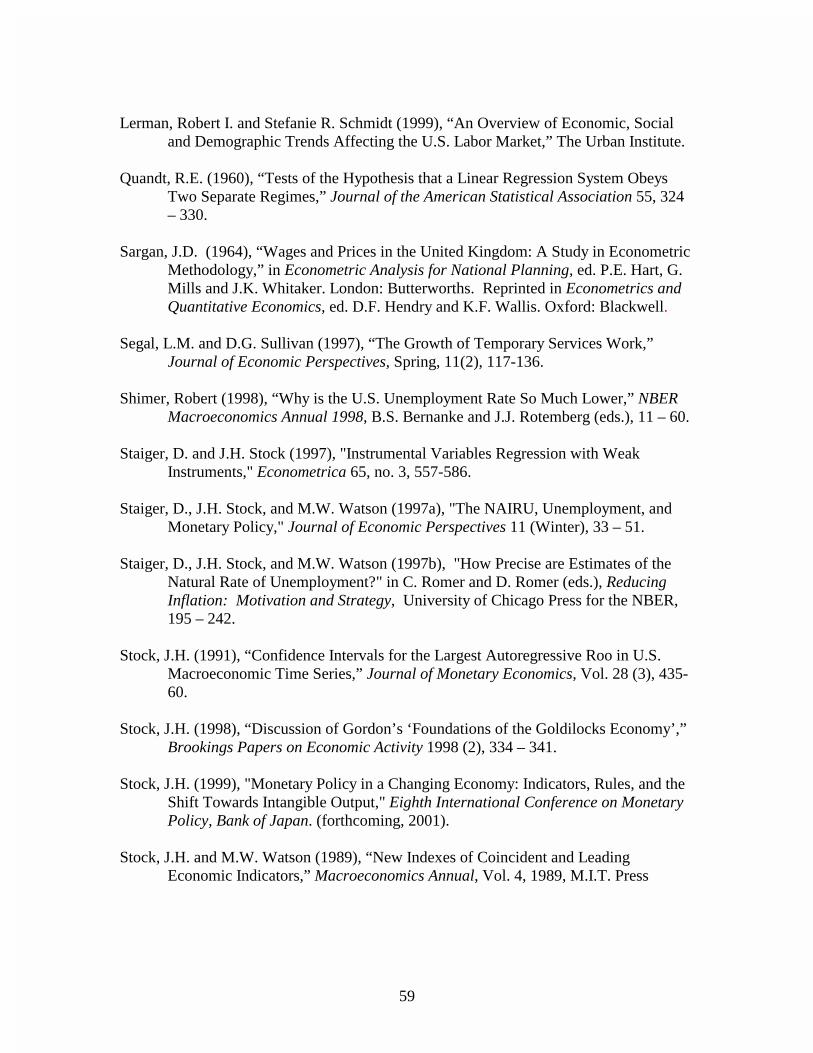
59

Lerman, Robert I. and Stefanie R. Schmidt (1999), “An Overview of Economic, Social

and Demographic Trends Affecting the U.S. Labor Market,” The Urban Institute. Quandt, R.E. (1960), “Tests of the Hypothesis that a Linear Regression System Obeys

Two Separate Regimes,” Journal of the American Statistical Association 55, 324 – 330.

Sargan, J.D. (1964), “Wages and Prices in the United Kingdom: A Study in Econometric

Methodology,” in Econometric Analysis for National Planning, ed. P.E. Hart, G. Mills and J.K. Whitaker. London: Butterworths. Reprinted in Econometrics and Quantitative Economics, ed. D.F. Hendry and K.F. Wallis. Oxford: Blackwell.

Segal, L.M. and D.G. Sullivan (1997), “The Growth of Temporary Services Work,”

Journal of Economic Perspectives, Spring, 11(2), 117-136. Shimer, Robert (1998), “Why is the U.S. Unemployment Rate So Much Lower,” NBER

Macroeconomics Annual 1998, B.S. Bernanke and J.J. Rotemberg (eds.), 11 – 60. Staiger, D. and J.H. Stock (1997), "Instrumental Variables Regression with Weak

Instruments," Econometrica 65, no. 3, 557-586. Staiger, D., J.H. Stock, and M.W. Watson (1997a), "The NAIRU, Unemployment, and

Monetary Policy," Journal of Economic Perspectives 11 (Winter), 33 – 51. Staiger, D., J.H. Stock, and M.W. Watson (1997b), "How Precise are Estimates of the

Natural Rate of Unemployment?" in C. Romer and D. Romer (eds.), Reducing Inflation: Motivation and Strategy, University of Chicago Press for the NBER, 195 – 242.

Stock, J.H. (1991), “Confidence Intervals for the Largest Autoregressive Roo in U.S.

Macroeconomic Time Series,” Journal of Monetary Economics, Vol. 28 (3), 435-60.

Stock, J.H. (1998), “Discussion of Gordon’s ‘Foundations of the Goldilocks Economy’,”

Brookings Papers on Economic Activity 1998 (2), 334 – 341. Stock, J.H. (1999), "Monetary Policy in a Changing Economy: Indicators, Rules, and the

Shift Towards Intangible Output," Eighth International Conference on Monetary Policy, Bank of Japan. (forthcoming, 2001).

Stock, J.H. and M.W. Watson (1989), “New Indexes of Coincident and Leading

Economic Indicators,” Macroeconomics Annual, Vol. 4, 1989, M.I.T. Press

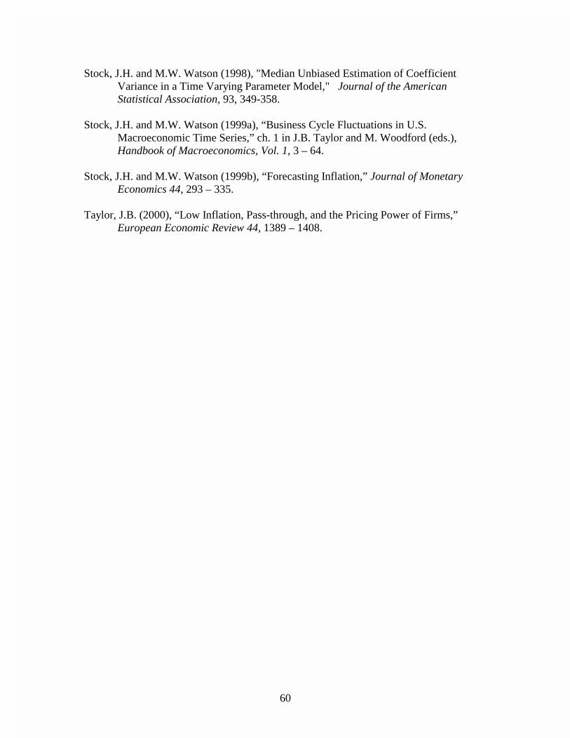
60

Stock, J.H. and M.W. Watson (1998), "Median Unbiased Estimation of Coefficient Variance in a Time Varying Parameter Model," Journal of the American Statistical Association, 93, 349-358.

Stock, J.H. and M.W. Watson (1999a), “Business Cycle Fluctuations in U.S.

Macroeconomic Time Series,” ch. 1 in J.B. Taylor and M. Woodford (eds.), Handbook of Macroeconomics, Vol. 1, 3 – 64.

Stock, J.H. and M.W. Watson (1999b), “Forecasting Inflation,” Journal of Monetary

Economics 44, 293 – 335. Taylor, J.B. (2000), “Low Inflation, Pass-through, and the Pricing Power of Firms,”

European Economic Review 44, 1389 – 1408.

Table 1

Descriptive Statistics for Trend Characteristics of the Data

Sample Mean Series

60:1-69:4

70:1-79:4

80:1 89:4

90:1-99:4

95% CI for the largest AR

root Price Inflation 2.47 6.50 4.46 2.23 0.90 to 1.02 Nominal Wage Growth Rate 4.95 8.05 5.36 3.72 0.91 to 1.02 Nominal Wage-Productivity Growth Rate

2.22 6.09 3.94 1.70 0.81 to 1.00

Real Wage1 Growth Rate 2.48 1.55 0.90 1.49 < 0.93 Real Wage2 Growth Rate 2.86 1.81 1.15 1.71 < 0.89 Real Wage1-Productivity Growth Rate

-0.25 -0.40 -0.52 -0.52 < 0.77

Real Wage2-Productivity Growth Rate

0.14 -0.15 -0.27 -0.30 < 0.77

Productivity Growth Rate 2.72 1.96 1.42 2.02 < 0.80 Real Wage1/Productivity (Log) -.029 -.067 -.080 -.138 0.97 to 1.03 Real Wage2/Productivity (Log) -.014 -.010 -.012 -.052 0.91 to 1.02 Unemployment Rate 4.78 6.21 7.27 5.76 0.89 to 1.02 Dem. Adj. Unemp. Rate 5.04 6.06 7.26 6.11 0.86 to 1.01 Building Permits (Log) 7.07 7.31 7.24 7.17 < 0.89 Capacity Utilization Rate 85.0 81.6 79.0 80.9 < 0.93 Notes: Columns 2-5 show the sample means of the series listed in the first column over the sample period indicated in the second row. The final column shows the 95 confidence for the largest root in a univariate AR(6) model (including the constant). The sample period for the regression was 1960:1-2000:2. The confidence interval was computed using the approximation developed in Stock (1991), for highly persistent series. Several of the series were not very persistent, and Stock’s method could only be used to compute an upper confidence bound. Real Wage1 uses price inflation computed from the GDP deflator, and Real Wage2 uses price inflation computed from the price deflator for the non-farm business sector.

Table 2

Phillips Curve Estimates from Macroeconomic Data Price Inflation Equation

∆πt+1 = βπ(ut-

Ntu ) + αππ(L)∆πt + απx(L)∆ut + γπZt + vπt+1

Civilian Unemployment

Rate

Demographically Adjusted

Unemployment Rate

Capacity Utilization

Building Permits

Phillips Curve Slope (SE)

[Stability P-value]

-0.28 (0.10 ) [0.06 ]

-0.26 (0.09 ) [0.13 ]

0.09 (0.03 ) [0.02 ]

2.18 (0.44 ) [0.16 ]

Trend Values

1970 4.33 4.39 85.51 7.27 1980 7.79 7.55 78.74 7.23 1990 6.40 6.66 80.84 7.18 2000 4.48 4.83 81.02 7.31

Change 1992-2000

-1.60 -1.59 -0.57 0.17

NAI Trend

Values (SE)

1970 4.62 ( 0.41 ) 4.66 ( 0.44 ) 84.86 ( 1.25 ) 7.23 ( 0.05 ) 1980 7.73 ( 0.39 ) 7.50 ( 0.42 ) 79.11 ( 1.20 ) 7.25 ( 0.05 ) 1990 6.38 ( 0.41 ) 6.65 ( 0.44 ) 80.86 ( 1.25 ) 7.18 ( 0.05 ) 2000 4.49 ( 0.54 ) 4.84 ( 0.58 ) 80.67 ( 1.65 ) 7.33 ( 0.07 )

Change 1992-2000

-1.60 ( 0.47 ) -1.59 ( 0.48 ) -0.88 ( 1.39 ) 0.18 ( 0.07 )

SER 0.92 0.93 0.94 0.91

TVP Std. Error (90% Conf. Int.)

0.026 (0.000 -0.114 )

0.023 (0.000 -0.106 )

0.024 (0.000 -0.107)

0.028 (0.000 -0.115 )

Notes: Results for the first column use the civilian unemployment rate as u in the estimated equation. The row labeled Phillips Curve Slope shows the estimates of βπ, with the standard error in parentheses, and the p-value of the QLR stability test in brackets. Trend Values are the (univariate) low-pass estimates of trend unemployment rate, and NAI Trend Values are the estimated values of the NAIRU computed using the Kalman smoother, as described in the text. SER is the standard error of the regression, and the TVP Std. Error is the median unbiased estimate of the standard deviation of the change in the equation’s constant term. The equation was estimated using 4 lags of ∆πt, two lags of ∆ut; the vector Z contained Gordon’s (1982) wage and price control variable, two lags of the relative price of food and energy and two lags of the exchange rate. The sample period is 1960:1-2000:2. Results in the remaining columns replace u with the demographically adjusted unemployment rate, capacity utilization and building permits.

Table 3 Alternative Phillips Curve Estimates from Macroeconomic Data

Price Inflation Equation

∆πt+1 = βπ(ut-Ntu ) + αππ(L)∆πt + απx(L)∆ut + αωω(L)(ωt–

*1tθ − –πt-1) + αωω (L)∆ωt + γπZt + vπt+1

Price Activity Np Na Ng Nr Nx Ne Nw Nm PC Slope SER TVPSE ∆ NAITV: median ub

∆ Intercept: median ub

∆ NAITV: 5%

∆Intercept: 5%

A. Baseline Specification (Table 1) GDP Def Civ. Unemp. 4 2 1 2 2 0 0 0 -0.28 (0.10 ) [0.06 ] 0.92 0.026 -1.60 ( 0.47 ) -0.00 ( 0.13 ) -1.62 ( 0.68 ) -0.01 ( 0.19 ) GDP Def Dem Adj. UR 4 2 1 2 2 0 0 0 -0.26 (0.09 ) [0.13 ] 0.93 0.023 -1.59 ( 0.48 ) -0.00 ( 0.12 ) -1.62 ( 0.75 ) -0.01 ( 0.19 ) GDP Def Cap. Util. 4 2 1 2 2 0 0 0 0.09 (0.03 ) [0.02 ] 0.94 0.024 -0.88 ( 1.39 ) 0.03 ( 0.13 ) -1.19 ( 2.14 ) 0.06 ( 0.19 ) GDP Def Bldg. Perm. 4 2 1 2 2 0 0 0 2.18 (0.44 ) [0.16 ] 0.91 0.028 0.18 ( 0.07 ) -0.02 ( 0.14 ) 0.20 ( 0.09 ) -0.05 ( 0.19 )

B. Different Price Indices PCE Def Civ. Unemp. 4 2 1 2 2 0 0 0 -0.28 (0.11 ) [0.20 ] 1.08 0.017 -1.61 ( 0.33 ) -0.00 ( 0.09 ) -1.59 ( 0.71 ) 0.00 ( 0.20 ) PCE Def Dem Adj. UR 4 2 1 2 2 0 0 0 -0.26 (0.11 ) [0.29 ] 1.09 0.015 -1.60 ( 0.31 ) -0.00 ( 0.08 ) -1.58 ( 0.75 ) 0.00 ( 0.20 ) PCE Def Cap. Util. 4 2 1 2 2 0 0 0 0.10 (0.03 ) [0.49 ] 1.07 0.020 -0.70 ( 1.08 ) 0.01 ( 0.11 ) -1.05 ( 1.95 ) 0.05 ( 0.20 ) PCE Def Bldg. Perm. 4 2 1 2 2 0 0 0 2.02 (0.54 ) [0.19 ] 1.08 0.021 0.18 ( 0.05 ) -0.01 ( 0.11 ) 0.19 ( 0.10 ) -0.03 ( 0.20 )

CPI Civ. Unemp. 4 2 1 2 2 0 0 0 -0.39 (0.14 ) [0.16 ] 1.34 0.000 -1.60 ( . ) 0.00 ( 0.00 ) -1.57 ( 0.53 ) 0.01 ( 0.20 ) CPI Dem Adj. UR 4 2 1 2 2 0 0 0 -0.37 (0.14 ) [0.19 ] 1.35 0.000 -1.59 ( . ) 0.00 ( 0.00 ) -1.56 ( 0.55 ) 0.01 ( 0.20 ) CPI Cap. Util. 4 2 1 2 2 0 0 0 0.15 (0.04 ) [0.19 ] 1.34 0.000 -0.57 ( 0.00 ) 0.00 ( 0.00 ) -1.04 ( 1.40 ) 0.07 ( 0.20 ) CPI Bldg. Perm. 4 2 1 2 2 0 0 0 3.63 (0.71 ) [0.05 ] 1.37 0.028 0.18 ( 0.04 ) -0.01 ( 0.15 ) 0.18 ( 0.06 ) -0.03 ( 0.20 )

C. Adding lags of wage inflation and error-correction term GDP Def Civ. Unemp. 4 2 1 2 2 1 4 0 -0.25 (0.10 ) [0.07 ] 0.91 0.026 -1.67 ( 0.55 ) -0.02 ( 0.14 ) -1.75 ( 0.77 ) -0.04 ( 0.19 ) GDP Def Dem Adj. UR 4 2 1 2 2 1 4 0 -0.23 (0.10 ) [0.16 ] 0.92 0.024 -1.65 ( 0.56 ) -0.01 ( 0.13 ) -1.76 ( 0.84 ) -0.04 ( 0.19 ) GDP Def Cap. Util. 4 2 1 2 2 1 4 0 0.09 (0.03 ) [0.02 ] 0.94 0.025 -0.74 ( 1.49 ) 0.02 ( 0.13 ) -0.83 ( 2.21 ) 0.02 ( 0.19 ) GDP Def Bldg. Perm. 4 2 1 2 2 1 4 0 2.05 (0.44 ) [0.20 ] 0.91 0.030 0.20 ( 0.07 ) -0.04 ( 0.15 ) 0.21 ( 0.09 ) -0.07 ( 0.19 )

D. Increasing lag length GDP Def Civ. Unemp. 8 4 1 2 2 0 0 0 -0.34 (0.12 ) [0.34 ] 0.89 0.052 * -1.71 ( 0.68 ) -0.04 ( 0.23 ) -1.66 ( 0.55 ) -0.02 ( 0.19 ) GDP Def Dem Adj. UR 8 4 1 2 2 0 0 0 -0.31 (0.12 ) [0.27 ] 0.91 0.050 * -1.70 ( 0.74 ) -0.03 ( 0.23 ) -1.66 ( 0.62 ) -0.02 ( 0.19 ) GDP Def Cap. Util. 8 4 1 2 2 0 0 0 0.10 (0.03 ) [0.00 ] 0.94 0.043 -1.15 ( 1.95 ) 0.06 ( 0.20 ) -1.10 ( 1.83 ) 0.06 ( 0.19 ) GDP Def Bldg. Perm. 8 4 1 2 2 0 0 0 2.29 (0.50 ) [0.23 ] 0.92 0.042 0.19 ( 0.09 ) -0.05 ( 0.20 ) 0.19 ( 0.08 ) -0.04 ( 0.19 ) GDP Def Civ. Unemp. 8 4 1 4 4 0 0 0 -0.34 (0.12 ) [0.42 ] 0.89 0.044 * -1.67 ( 0.60 ) -0.02 ( 0.21 ) -1.65 ( 0.56 ) -0.02 ( 0.19 ) GDP Def Dem Adj. UR 8 4 1 4 4 0 0 0 -0.31 (0.12 ) [0.33 ] 0.91 0.041 -1.65 ( 0.65 ) -0.02 ( 0.20 ) -1.65 ( 0.62 ) -0.02 ( 0.19 ) GDP Def Cap. Util. 8 4 1 4 4 0 0 0 0.11 (0.03 ) [0.01 ] 0.94 0.036 -1.06 ( 1.69 ) 0.05 ( 0.18 ) -1.11 ( 1.81 ) 0.06 ( 0.19 ) GDP Def Bldg. Perm. 8 4 1 4 4 0 0 0 2.25 (0.51 ) [0.38 ] 0.92 0.043 0.20 ( 0.09 ) -0.05 ( 0.20 ) 0.19 ( 0.09 ) -0.04 ( 0.19 )

E. Eliminating RPFE ExRates and W&P Control Variables GDP Def Civ. Unemp. 4 2 0 0 0 0 0 0 -0.37 (0.10 ) [0.08 ] 1.00 0.048 -1.55 ( 0.61 ) 0.02 ( 0.23 ) -1.56 ( 0.53 ) 0.01 ( 0.19 ) GDP Def Dem Adj. UR 4 2 0 0 0 0 0 0 -0.34 (0.10 ) [0.17 ] 1.02 0.048 -1.53 ( 0.67 ) 0.02 ( 0.23 ) -1.55 ( 0.57 ) 0.01 ( 0.20 ) GDP Def Cap. Util. 4 2 0 0 0 0 0 0 0.11 (0.03 ) [0.05 ] 1.02 0.050 * -1.40 ( 2.09 ) 0.09 ( 0.23 ) -1.17 ( 1.74 ) 0.07 ( 0.20 ) GDP Def Bldg. Perm. 4 2 0 0 0 0 0 0 1.78 (0.44 ) [0.24 ] 1.03 0.031 0.18 ( 0.09 ) -0.01 ( 0.16 ) 0.18 ( 0.11 ) -0.01 ( 0.20 )

F. Adding Markup Variable GDP Def Civ. Unemp. 4 2 1 2 2 0 0 2 -0.27 (0.09 ) [0.09 ] 0.91 0.035 -1.43 ( 0.65 ) 0.05 ( 0.17 ) -1.41 ( 0.72 ) 0.05 ( 0.19 ) GDP Def Dem Adj. UR 4 2 1 2 2 0 0 2 -0.24 (0.09 ) [0.19 ] 0.92 0.035 -1.40 ( 0.73 ) 0.05 ( 0.17 ) -1.38 ( 0.80 ) 0.05 ( 0.19 ) GDP Def Cap. Util. 4 2 1 2 2 0 0 2 0.09 (0.03 ) [0.02 ] 0.93 0.023 -0.96 ( 1.41 ) 0.03 ( 0.12 ) -1.36 ( 2.24 ) 0.07 ( 0.19 )

GDP Def Bldg. Perm. 4 2 1 2 2 0 0 2 2.08 (0.44 ) [0.26 ] 0.90 0.025 0.16 ( 0.06 ) 0.02 ( 0.13 ) 0.16 ( 0.09 ) 0.03 ( 0.19 ) GDP Def Civ. Unemp. 8 4 1 2 2 0 0 2 -0.32 (0.12 ) [0.34 ] 0.89 0.043 * -1.44 ( 0.64 ) 0.05 ( 0.20 ) -1.45 ( 0.60 ) 0.05 ( 0.19 ) GDP Def Dem Adj. UR 8 4 1 2 2 0 0 2 -0.28 (0.12 ) [0.27 ] 0.90 0.040 -1.43 ( 0.69 ) 0.05 ( 0.19 ) -1.43 ( 0.68 ) 0.05 ( 0.19 ) GDP Def Cap. Util. 8 4 1 2 2 0 0 2 0.10 (0.03 ) [0.01 ] 0.93 0.036 -1.18 ( 1.80 ) 0.06 ( 0.18 ) -1.25 ( 1.94 ) 0.07 ( 0.19 ) GDP Def Bldg. Perm. 8 4 1 2 2 0 0 2 2.20 (0.50 ) [0.28 ] 0.91 0.032 0.16 ( 0.07 ) 0.03 ( 0.16 ) 0.16 ( 0.09 ) 0.03 ( 0.19 )

Notes: This table contains alternative estimates of the price Phillips Curve equation and the TV NAIRU. The first column shows the price series used to construct π, and the second column shows the activity variable used for u. The next columns shows a set of parameters that described the specification: Np = number of lags of inflation, Na = number of lags of activity variable, Ng is a binary variable indicating inclusion(1)/exclusion(0) of Wage and Price Variable (Gordon (1982)), Nr = number of lags of the relative price of food and energy, Nx = number of lags of exchange rates, Ne is a binary variable indicating inclusion(1)/exclusion(0) of the wage/price/productivity error correction term (ωt–

*1tθ − –πt-1), Nw = number of lags of ∆ω, and Nm=number of lags of markup variable

described in the text. The next three columns are described in the notes to Table 1. An asterisk in the column labeled TVPSE indicates that the estimated TVPSE is significantly different from 0 at the 5% level. The columns labeled ∆ NAITV show the change in the NAIRU (or the NAI trend value) from 1992:1-2000:1, and the columns labeled ∆ Intercept show the implied in the equation’s constant term over the same period. These are presented for two value of the standard error of the change in the constant: the median unbiased estimate (shown in column (6)), and a value of .039 (which implies a standard deviation of the change in the constant of 5% over the sample period.) The sample period is 1960:1-2000:1 for all estimated equations.

Table 4 Phillips Curve Estimates from Macroeconomic Data

Wage Inflation Equation

ωt+1–*tθ –πt = βω(ut-

Ntu ) + αωπ(L)∆πt + αωω(L)(ωt–

*1tθ − –πt-1) + αωu(L)∆ut + vωt+1

Civilian

Unemployment Rate

Demographically Adjusted

Unemployment Rate

Capacity Utilization

Building Permits

Phillips Curve Slope (SE)

[Stability P-value]

-0.42 (0.19 ) [0.10 ]

-0.39 (0.18 ) [0.10 ]

0.11 (0.05 ) [0.29 ]

2.00 (0.78 ) [0.99 ]

Trend Values

1970 4.33 4.39 85.51 7.27 1980 7.79 7.55 78.74 7.23 1990 6.40 6.66 80.84 7.18 2000 4.48 4.83 81.02 7.31

Change 1992-2000

-1.60 -1.59 -0.57 0.17

NAI Trend Values

1970 3.75 ( 0.46 ) 3.72 ( 0.49 ) 88.61 ( 1.37 ) 7.40 ( 0.10 ) 1980 6.98 ( 0.43 ) 6.67 ( 0.46 ) 81.92 ( 1.34 ) 7.41 ( 0.09 ) 1990 5.39 ( 0.46 ) 5.58 ( 0.49 ) 84.09 ( 1.37 ) 7.40 ( 0.10 ) 2000 3.54 ( 0.58 ) 3.80 ( 0.61 ) 84.26 ( 1.43 ) 7.52 ( 0.12 )

Change 1992-2000

-1.52 ( 0.43 ) -1.52 ( 0.43 ) -0.59 ( 0.45 ) 0.16 ( 0.09 )

SER 1.81 1.81 1.82 1.81

TVP Std. Error (90% Conf. Int.)

0.034 (0.000 -0.186)

0.031 (0.000 -0.182)

0.009 (0.000 -0.150

0.034 (0.000 -0.187

Notes: The equation was estimated using 4 lags of ∆πt, 4 lags of (ωt–*

1tθ − –πt-1) and two lags of

∆ut. See notes to table 1 for a description of the table entries.

Table 5 Alternative Phillips Curve Estimates from Macroeconomic Data

Wage Inflation Equation

ωt+1–*tθ –πt = βω(ut-

Ntu ) + αωπ(L)∆πt + αωω(L)(ωt–

*1tθ − –πt-1) + αωu(L)∆ut + vωt+1

Wage Price Activity Nw Na Np Pr PC Slope SER TVPSE ∆ NAITV: median ub

∆ Intercept: median ub

∆ NAITV: 5%

∆ Intercept: 5%

A. Baseline Specification (Table 3) Comp/Hr GDP Def Civ. Unemp. 4 2 4 2 -0.42 (0.19 ) [0.10 ] 1.81 0.034 -1.52 ( 0.43 ) 0.03 ( 0.18 ) -1.49 ( 0.50 ) 0.05 ( 0.21 ) Comp/Hr GDP Def Dem Adj. UR 4 2 4 2 -0.39 (0.18 ) [0.10 ] 1.81 0.031 -1.52 ( 0.43 ) 0.03 ( 0.17 ) -1.47 ( 0.54 ) 0.05 ( 0.21 ) Comp/Hr GDP Def Cap. Util. 4 2 4 2 0.11 (0.05 ) [0.29 ] 1.82 0.009 -0.59 ( 0.45 ) 0.00 ( 0.05 ) -1.18 ( 1.93 ) 0.07 ( 0.21 ) Comp/Hr GDP Def Bldg. Perm. 4 2 4 2 2.01 (0.78 ) [0.99 ] 1.81 0.034 0.16 ( 0.09 ) 0.03 ( 0.19 ) 0.15 ( 0.10 ) 0.04 ( 0.21 ) B. Alternative productivity trends

Comp/Hr GDP Def Civ. Unemp. 4 2 4 1 -0.42 (0.19 ) [0.14 ] 1.86 0.102 * -0.76 ( 1.10 ) 0.35 ( 0.47 ) -1.42 ( 0.50 ) 0.07 ( 0.21 ) Comp/Hr GDP Def Dem Adj. UR 4 2 4 1 -0.38 (0.19 ) [0.13 ] 1.86 0.101 * -0.67 ( 1.22 ) 0.35 ( 0.46 ) -1.40 ( 0.55 ) 0.07 ( 0.21 ) Comp/Hr GDP Def Cap. Util. 4 2 4 1 0.12 (0.05 ) [0.56 ] 1.87 0.090 * -3.73 ( 3.59 ) 0.37 ( 0.42 ) -1.36 ( 1.79 ) 0.09 ( 0.21 ) Comp/Hr GDP Def Bldg. Perm. 4 2 4 1 1.79 (0.81 ) [0.84 ] 1.87 0.076 0.04 ( 0.21 ) 0.23 ( 0.37 ) 0.13 ( 0.12 ) 0.07 ( 0.21 ) Comp/Hr GDP Def Civ. Unemp. 4 2 4 3 -0.40 (0.19 ) [0.33 ] 1.80 0.056 -1.57 ( 0.73 ) 0.01 ( 0.29 ) -1.61 ( 0.53 ) -0.00 ( 0.21 ) Comp/Hr GDP Def Dem Adj. UR 4 2 4 3 -0.36 (0.18 ) [0.32 ] 1.80 0.056 -1.56 ( 0.79 ) 0.01 ( 0.29 ) -1.60 ( 0.58 ) -0.00 ( 0.21 ) Comp/Hr GDP Def Cap. Util. 4 2 4 3 0.11 (0.05 ) [0.21 ] 1.81 0.046 -0.81 ( 2.21 ) 0.03 ( 0.24 ) -0.72 ( 1.94 ) 0.02 ( 0.21 ) Comp/Hr GDP Def Bldg. Perm. 4 2 4 3 1.84 (0.78 ) [0.75 ] 1.81 0.058 0.17 ( 0.16 ) -0.00 ( 0.30 ) 0.18 ( 0.11 ) -0.01 ( 0.21 )

C. Alternative price indices Comp/Hr NFB Def Civ. Unemp. 4 2 4 2 -0.36 (0.19 ) [0.24 ] 1.87 0.025 -1.58 ( 0.38 ) 0.01 ( 0.14 ) -1.52 ( 0.59 ) 0.03 ( 0.21 ) Comp/Hr NFB Def Dem Adj. UR 4 2 4 2 -0.32 (0.18 ) [0.24 ] 1.87 0.015 -1.58 ( 0.27 ) 0.00 ( 0.09 ) -1.50 ( 0.66 ) 0.03 ( 0.21 ) Comp/Hr NFB Def Cap. Util. 4 2 4 2 0.11 (0.05 ) [0.43 ] 1.88 0.000 -0.57 ( 0.00 ) 0.00 ( 0.00 ) -1.08 ( 2.00 ) 0.05 ( 0.21 ) Comp/Hr NFB Def Bldg. Perm. 4 2 4 2 2.94 (0.84 ) [0.78 ] 1.84 0.017 0.17 ( 0.03 ) 0.00 ( 0.09 ) 0.17 ( 0.07 ) 0.02 ( 0.21 ) Comp/Hr PCE Def Civ. Unemp. 4 2 4 2 -0.29 (0.19 ) [0.10 ] 1.84 0.088 * -0.78 ( 1.42 ) 0.24 ( 0.42 ) -1.43 ( 0.72 ) 0.05 ( 0.21 ) Comp/Hr PCE Def Dem Adj. UR 4 2 4 2 -0.26 (0.18 ) [0.10 ] 1.84 0.086 -0.71 ( 1.56 ) 0.23 ( 0.41 ) -1.40 ( 0.81 ) 0.05 ( 0.21 ) Comp/Hr PCE Def Cap. Util. 4 2 4 2 0.08 (0.05 ) [0.50 ] 1.84 0.074 -3.61 ( 4.72 ) 0.23 ( 0.36 ) -1.45 ( 2.73 ) 0.07 ( 0.21 ) Comp/Hr PCE Def Bldg. Perm. 4 2 4 2 1.73 (0.83 ) [0.89 ] 1.83 0.087 0.05 ( 0.24 ) 0.22 ( 0.41 ) 0.15 ( 0.12 ) 0.05 ( 0.21 ) Comp/Hr CPI Civ. Unemp. 4 2 4 2 -0.17 (0.20 ) [0.13 ] 1.85 0.098 * -0.86 ( 2.59 ) 0.13 ( 0.45 ) -1.53 ( 1.21 ) 0.01 ( 0.21 ) Comp/Hr CPI Dem Adj. UR 4 2 4 2 -0.15 (0.19 ) [0.12 ] 1.85 0.095 * -0.78 ( 2.97 ) 0.12 ( 0.44 ) -1.51 ( 1.41 ) 0.01 ( 0.21 ) Comp/Hr CPI Cap. Util. 4 2 4 2 0.06 (0.06 ) [0.71 ] 1.86 0.085 -3.27 ( 6.83 ) 0.16 ( 0.41 ) -1.09 ( 3.54 ) 0.03 ( 0.21 ) Comp/Hr CPI Bldg. Perm. 4 2 4 2 2.04 (0.87 ) [0.78 ] 1.83 0.109 * 0.13 ( 0.24 ) 0.08 ( 0.49 ) 0.17 ( 0.10 ) -0.00 ( 0.21 )

D. Alternative wage indices AHE PW GDP Def Civ. Unemp. 4 2 4 5 -0.15 (0.12 ) [0.55 ] 1.12 0.077 * -1.33 ( 2.18 ) 0.04 ( 0.33 ) -1.46 ( 1.32 ) 0.02 ( 0.20 ) AHE PW GDP Def Dem Adj. UR 4 2 4 5 -0.14 (0.12 ) [0.48 ] 1.13 0.077 * -1.29 ( 2.31 ) 0.04 ( 0.33 ) -1.44 ( 1.39 ) 0.02 ( 0.20 ) AHE PW GDP Def Cap. Util. 4 2 4 5 0.04 (0.03 ) [0.35 ] 1.11 0.061 * -1.89 ( 6.85 ) 0.05 ( 0.28 ) -1.33 ( 4.86 ) 0.03 ( 0.20 ) AHE PW GDP Def Bldg. Perm. 4 2 4 5 1.08 (0.55 ) [0.70 ] 1.11 0.086 * 0.17 ( 0.33 ) 0.00 ( 0.35 ) 0.17 ( 0.18 ) 0.00 ( 0.20 )

Comp/Hr Man GDP Def Civ. Unemp. 4 2 4 5 -0.50 (0.21 ) [0.45 ] 2.01 0.141 * -1.69 ( 1.20 ) -0.05 ( 0.60 ) -1.71 ( 0.43 ) -0.05 ( 0.21 ) Comp/Hr Man GDP Def Dem Adj. UR 4 2 4 5 -0.47 (0.21 ) [0.45 ] 2.02 0.140 * -1.69 ( 1.27 ) -0.05 ( 0.60 ) -1.70 ( 0.45 ) -0.05 ( 0.21 ) Comp/Hr Man GDP Def Cap. Util. 4 2 4 5 0.13 (0.06 ) [0.44 ] 2.04 0.137 * -1.19 ( 4.57 ) 0.08 ( 0.59 ) -0.29 ( 1.65 ) -0.04 ( 0.21 ) Comp/Hr Man GDP Def Bldg. Perm. 4 2 4 5 0.98 (0.92 ) [0.92 ] 2.06 0.146 * 0.14 ( 0.63 ) 0.03 ( 0.62 ) 0.22 ( 0.22 ) -0.04 ( 0.21 )

ECC-C GDP Def Civ. Unemp. 4 2 4 2 -0.14 (0.11 ) [0.33 ] 0.58 0.000 -1.60 ( 0.00 ) 0.00 ( 0.00 ) -1.27 ( 1.22 ) 0.05 ( 0.17 )

ECC-C GDP Def Dem Adj. UR 4 2 4 2 -0.12 (0.10 ) [0.37 ] 0.58 0.000 -1.59 ( 0.00 ) 0.00 ( 0.00 ) -1.24 ( 1.37 ) 0.04 ( 0.17 ) ECC-C GDP Def Cap. Util. 4 2 4 2 0.03 (0.04 ) [0.01 ] 0.59 0.000 -0.57 ( 0.00 ) 0.00 ( 0.00 ) -4.38 ( 6.30 ) 0.10 ( 0.17 ) ECC-C GDP Def Bldg. Perm. 4 2 4 2 0.99 (0.55 ) [0.66 ] 0.58 0.000 0.17 ( 0.00 ) 0.00 ( 0.00 ) 0.14 ( 0.17 ) 0.04 ( 0.17 )

ECC-WS GDP Def Civ. Unemp. 4 2 4 2 -0.06 (0.12 ) [0.10 ] 0.76 0.106 * 5.16 ( 5.83 ) 0.39 ( 0.34 ) 1.52 ( 3.17 ) 0.18 ( 0.18 ) ECC-WS GDP Def Dem Adj. UR 4 2 4 2 -0.07 (0.12 ) [0.15 ] 0.76 0.104 * 4.35 ( 5.06 ) 0.39 ( 0.33 ) 1.18 ( 2.78 ) 0.18 ( 0.18 ) ECC-WS GDP Def Cap. Util. 4 2 4 2 0.03 (0.05 ) [0.82 ] 0.77 0.088 * -10.64 ( 9.08 ) 0.34 ( 0.31 ) -5.62 ( 5.43 ) 0.17 ( 0.18 ) ECC-WS GDP Def Bldg. Perm. 4 2 4 2 2.02 (0.72 ) [0.10 ] 0.73 0.130 * -0.06 ( 0.18 ) 0.47 ( 0.36 ) 0.06 ( 0.09 ) 0.22 ( 0.18 )

E. Increasing lag length Comp/Hr GDP Def Civ. Unemp. 8 4 8 2 -0.49 (0.25 ) [0.05 ] 1.79 0.055 -1.37 ( 0.57 ) 0.11 ( 0.28 ) -1.48 ( 0.43 ) 0.06 ( 0.21 ) Comp/Hr GDP Def Dem Adj. UR 8 4 8 2 -0.45 (0.24 ) [0.06 ] 1.81 0.053 -1.35 ( 0.62 ) 0.10 ( 0.28 ) -1.46 ( 0.47 ) 0.06 ( 0.21 ) Comp/Hr GDP Def Cap. Util. 8 4 8 2 0.12 (0.07 ) [0.33 ] 1.81 0.029 -0.91 ( 1.29 ) 0.04 ( 0.16 ) -1.19 ( 1.70 ) 0.08 ( 0.21 ) Comp/Hr GDP Def Bldg. Perm. 8 4 8 2 2.47 (0.92 ) [0.79 ] 1.82 0.027 0.16 ( 0.06 ) 0.02 ( 0.15 ) 0.15 ( 0.09 ) 0.05 ( 0.21 ) F. Eliminating lags of price inflation Comp/Hr GDP Def Civ. Unemp. 4 2 0 2 -0.12 (0.17 ) [0.01 ] 1.93 0.000 -1.60 ( 0.00 ) 0.00 ( 0.00 ) -1.16 ( 1.72 ) 0.05 ( 0.21 ) Comp/Hr GDP Def Dem Adj. UR 4 2 0 2 -0.09 (0.17 ) [0.01 ] 1.93 0.000 -1.59 ( 0.00 ) 0.00 ( 0.00 ) -0.97 ( 2.46 ) 0.05 ( 0.21 ) Comp/Hr GDP Def Cap. Util. 4 2 0 2 0.01 (0.05 ) [0.22 ] 1.93 0.000 -0.57 ( 0.00 ) 0.00 ( 0.00 ) -6.79 (23.06 ) 0.06 ( 0.21 ) Comp/Hr GDP Def Bldg. Perm. 4 2 0 2 1.07 (0.78 ) [0.85 ] 1.91 0.000 0.17 ( 0.00 ) 0.00 ( 0.00 ) 0.13 ( 0.20 ) 0.04 ( 0.21 )

Notes: Notes: This table contains alternative estimates of the wage Phillips Curve equation and the TV NAIRU. The first column shows the wage series used to construct ω, the next column shows price series used to construct π and the third column shows the activity variable used for u. The next columns shows a set of parameters that described the specification: Nw= number of lags of real wages, Np = number of lags of inflation, Na = number of lags of activity variable, Pr = trend estimate of productivity growth (1=Average value of NFB productivity growth, 1960-2000; 2=low-pass filter of NFB productivity growth using I(0) AR extrapolation; 3=low-pass filter of NFB productivity growth using I(1) AR extrapolation; 5=2=low-pass filter of manufacturing productivity growth using I(0) AR extrapolation). The remaining columns are described in the notes to Table 2. The sample period is 1960:1-2000:1 for all estimated equations except those including ECC-C and ECC-WS, which used the sample period 1982:1-2000:1.

Table 6

Phillips Curve Estimates from State Data

ωit+1–θit+1–πt+1 = αi + δt + βuit + vit+1 OLS IV Phillips Curve Slope (SE) -0.165

(0.045) -0.409 (0.070)

-0.208 (.061)

-0.586 (0.113)

Year Effects P-Value

0.00 0.00 0.00 0.00

State Effects P-value

Excluded 0.81 Excluded 0.94

R2 0.26 0.29 NA NA Notes: N=912 (1979-1997). IV estimates use even months of MORG as instrument for odd months.

Table 7 Alternative Phillips Curve Estimates

ωit+1–θit+1–πt+1 = αi + δt + βuit + vit+1

Deviation of Specification from Benchmark PC Slope (SE) (0) None -0.586 (0.113) (1) IV Odd month IV for Even Months -0.447 (0.113) (2) Weighting by Size of State Workforce -0.542 (0.089) (3) Adjusted Wages2 and Unemployment Rate1 -0.506 (0.097) (4) Adjusted Unemployment Rate1 -0.535 (0.111) (5) Adjusted Unemployment Rate2 -0.534 (0.129) (6) Adjusted Wages2 -0.552 (0.098) (7) Wages – Median/All -0.625 (0.151) (8) Wages – Mean/Full Time -0.526 (0.128) (9) Wages – Mean/Hourly -0.660 (0.119) (10) Productivity Growth Omitted -0.637 (0.092) (11) Productivity Growth Uses as a Regressor -0.654 (0.094) (12) Weighted Industry Productivity Growth -0.718 (0.095) (13) Productivity Growth dated “t” -0.418 (0.114) (14) Unemployment dated “t+1” -0.385 (0.112) Notes: The table shows estimates of the Phillips curve slope and associated standard error for alternative specifications. The first column describes the deviation from the benchmark model (given in the last column of table 6 and labeled (0) in this table). Specification (1) reverses the role of instruments and regressors in the baseline specification. Specification (2) uses weighted IV, where the weights are the size of the state workforce. Specifications (3)-(6) use adjusted values for wages and/or the unemployment rate. Variables with a “1” subscript were adjusted using cross-section regressions each year that controlled for 10 education categories, 3 race categories, a quartic in potential experience, and an interaction between gender and all other regressors. Variables with a “2” subscript used these regressors together with 11 major industry indicator variables. Specifications (7)-(9) use alternative wage measures: Median hourly wage for all workers, mean hourly wage for full-time workers, and mean hourly wage for workers paid on hourly basis. Specification (10) uses the dependent variables ωti+1-πt+1, (11) adds θit+1 as a regressor (relaxing the unit elasticity constraint), and (12) uses a weighted industry measure of state productivity growth. Specification (13) used the dependent variable ωit+1–θit–πt+1 , and specification (14) uses uit+1 as the regressor. (The results are invariant to the timing of πt because of the include or time effects.) The sample period for Specification (10) was 1979-98 (N=960), and was 1979-97 (N=912) for all other specifications.

Table 8 Alternate Specification of Phillips Curve Dynamics

A. Relaxing the Unit Root Constraint on Real Wages

ωit+1–θit+1–πt+1 = αi + δt + βuit + γ[ln(Wit/Pt) – ln(Productivityit)] + vit+1

Variable OLS IV Unemployment

Rate -0.401 (.065)

-0.375 (.062)

-0.480 (.049)

-0.581 (.113)

-0.548 (.097)

-0.612 (.089)

Real Wage -0.103

(.021) -0.090 (.022)

-0.146 (.015)

-.010 (.034)

-0.028 (.030)

-0.057 (.026)

Productivity Adjustment

Yes Yes No Yes Yes No

Adjusted Wages2 No Yes No No Yes No

Notes: Specifications with “No” productivity adjustment omit the terms θit+1 from the dependent variable and ln(Productivityit) from the regressor. See notes to table 7 for the definition of Adjusted Wages2. B. Allowing Distributed Lags

ωit+1–θit+1–πt+1 = αi + δt + βuit + αω(L)[ωit-θit-πt] + αu(L)∆ut + vit+1

Variable Coefficient (SE) uit -0.486 (.131) -0.549 (.161) ωit-θit-πt 0.051 (.103) 0.031 (.107) ωit-1-θit-1-πt-1 -0.210 (.094) ∆ut -0.404 (.345) -0.141 (.411) ∆ut-1 -0.020 (.520)

P-Value for αω(L)=0 .62 .08 P-Value for αu(L)=0 .24 .86 Notes: The sample period is 1981-97 (N=816)

Table 9: Stability of Phillips Curve through Time and Space

ωit+1–θit+1–πt+1 = αi + δt + βit uit + vit+1

Variable Coefficient (SE)

uit -0.586 (.113) -0.623 (.142) -0.736 (.139) uit � 1(tr1984) 0.066 (.143) uit� 1(tr1992) 0.014 (.204) uit � 1(i in Northeast) 0.509 (.198) uit � 1(i in North Central) 0.065 (.159) uit � 1(i in West) 0.214 (.203) Temporal Stability p-Value 0.895 Spatial Stability p-Value 0.065 Notes: The sample period is 1979-1997 (N=912). The temporal stability p-value is associated with the Wald test for the hypothesis that the coefficients on uit interacted with the time indicators are zero. The spatial stability p-value is associated with the Wald test for the hypothesis that the coefficients on uit interacted with the region indicators are zero.

Table 10 Demographic Variables and the Phillips Curve

ωit+1–θit+1–πt+1 = αi + δt + β uit + γ Xit + vit+1

Variable Coefficient (SE)

Unemployment rate -0.586 (.113)

-0.642 (.147)

-0.550 (.134)

-0.604 (.120)

-0.542 (.159)

-0.526 (.320)

%High School Dropout -0.099 (.140)

-0.081 (.189)

%College Graduate 0.299 (.345)

0.577 (.918)

%White 0.233 (.543)

0.164 (2.000)

%Female -0.328 (.621)

0.030 (1.378)

%Age 25-54 -0.113 (.285)

-0.381 (.981)

Education Variables p-Value 0.339 0.704 All Demographics p-Value 0.712 Notes: The sample period is 1979-97 (N=912).

Table 11 Industry Characteristics and the Phillips Curve

ωit+1–θit+1–πt+1 = αi + δt + β uit + γ Xit + vit+1

Variable Coefficient (SE) Unemployment rate

-0.586 (.113)

-0.823 (.170)

-1.084 (.397)

-0.599 (.115)

-0.575 (.115)

-0.854 (.179)

%Durable Mfg. 0.333 (.227)

0.196 (.283)

%Non-durable Mfg.

-0.166 (.303)

-0.247 (.312)

%Retail Trade 0.275 (.708)

0.161 (.715)

%Services 1.045 (.501)

1.113 (.526)

%Temp Help (CPS)

-19.239 (13.567)

%Temp Help (CBP)

-0.290 (.324)

-0.159 (.383)

%Self-Employed

-0.196 (.272)

-0.437 (.487)

Major Industry p-Value 0.153 0.164 All Industry Variables p-Value 0.312 Notes: The sample period is 1979-97 (N=912).

Table 12 Government Policy Variables and the Phillips Curve

ωit+1–θit+1–πt+1 = αi + δt + β uit + γ Xit + vit+1

Variable Coefficient (SE) Unemployment rate -0.586 (.113) -0.576 (.120) -0.603 (.114) -0.591 (.114) -0.600 (.122) %Of 25-64 on DI 0.360 (.606) 0.376 (.611) %Of 25-64 on SSI 0.046 (.577) 0.025 (.578) Minimum Wage (99$) -0.414 (.864) -0.354 (.879) %Growth in Min. Wage -0.085 (.049) -0.084 (.049) UI Replacement Rate 0.015 (.043) 0.017 (.043) DI/SSI Variables p-Value 0.746 0.749 Min. Wage Variables p-Value 0.207 0.210 All Policy Variables p-Value 0.566 Notes: The sample period is 1979-97 (N=912).

Figure 1aPrice Inflation and Unemployment

-4

-3

-2

-1

0

1

2

3

4

2 3 4 5 6 7 8 9 10

Unemployment Rate (t)

Infl

atio

n C

han

ge

bet

wee

n (

t) a

nd

(t+

1)

9398

97

96 95

94

1960-1992 Regression Line

Shifted PC 1993-1998

1993-1998 Regression Line

Figure 1bReal Wage Inflation and Unemployment

-3

-2

-1

0

1

2

3

4

5

2 3 4 5 6 7 8 9 10

Unemployment Rate (t)

Infl

atio

n C

han

ge

bet

wee

n (

t) a

nd

(t+

1)

93

98

97

9695

94

1960-1992 Regression Line

Shifted PC 1993-1998

1993-1998 Regression Line

Average Labor Productivity Growth Rate

Figure 3NAIRU From Price Phillips Curve

0

2

4

6

8

10

12

1960 1965 1970 1975 1980 1985 1990 1995 2000

Year

Per

cen

t

Unemployment Rate

NAIRU Estimate

Trend Unemployment

± 2 SE Bands for NAIRU

Figure 4Slope from Baseline Price Phillips Curve

-1

-0.8

-0.6

-0.4

-0.2

0

0.2

0.4

0.6

1960 1965 1970 1975 1980 1985 1990 1995 2000

Year

Slo

pe

Co

effi

cien

t

OLS Estimate

TVP Estimate

± 2 SE Bands for TV Slope

Figure 5NAIRU From Wage Phillips Curve

0

2

4

6

8

10

12

1960 1965 1970 1975 1980 1985 1990 1995 2000

Year

Per

cen

t

Unemployment Rate

NAIRU Estimate

Trend Unemployment

± 2 SE Bands for NAIRU

Figure 6Slope from Baseline Wage Phillips Curve

-1.6

-1.4

-1.2

-1

-0.8

-0.6

-0.4

-0.2

0

0.2

0.4

0.6

0.8

1

1960 1965 1970 1975 1980 1985 1990 1995 2000

Year

Slo

pe

Co

effi

cien

t

OLS Estimate

TVP Estimate

± 2 SE Bands for TV Slope

Figure 7State Estimates of TV NAIRU

4

6

8

10

1979 1980 1981 1982 1983 1984 1985 1986 1987 1988 1989 1990 1991 1992 1993 1994 1995 1996 1997 1998

Year

Per

cen

t

Unemployment Rate

Trend Unemployment Rate

NAIRU Without Productivity

NAIRU With Productivity

Figure 8aTrend Unemployment and Productivity Growth

0

1

2

3

4

5

6

7

8

9

1960 1965 1970 1975 1980 1985 1990 1995 2000

Year

Per

cen

t

Unemployment Rate Trend

Productivity Growth Trend

Figure 8bUnemployment Rate and Productivity Growth Trends

0

0.5

1

1.5

2

2.5

3

3.5

3 4 5 6 7 8 9

Unemployment Rate

Pro

du

ctiv

ity

Gro

wth

1967:III

1960:I

1980:III

2000:II

1993:I