Pricing Default Risk: The Good, The Bad, and The Anomaly

Munich Personal RePEc Archive

Pricing Default Risk: The Good, The

Bad, and The Anomaly

Ferreira Filipe, Sara and Grammatikos, Theoharry and

Michala, Dimitra

University of Luxembourg, University of Luxembourg, University of

Luxembourg

1 February 2014

Online at https://mpra.ub.uni-muenchen.de/53373/

MPRA Paper No. 53373, posted 04 Feb 2014 17:07 UTC

Pricing Default Risk: The Good, The Bad, and The Anomaly

Sara Ferreira Filipe*, Theoharry Grammatikos*, Dimitra Michala*

Luxembourg School of Finance

February 2014

ABSTRACT

While the empirical literature has often documented a “default anomaly”, i.e. a negative relation

between default risk and stock returns, standard theory suggests that default risk should be priced

in the cross-section. In this paper, we provide an explanation for this apparent puzzle using a new

approach. First we calculate monthly physical probabilities of default (PDs) for a large sample of

European firms. Second we decompose these estimated PDs into systematic and idiosyncratic

components; we measure the systematic part as the sensitivity of the physical PD to an aggregate

measure of default risk. While sorting stocks based on physical PDs confirms a possible default

anomaly, we find that the relation between the systematic default risk and stock returns is in fact

positive. Our results therefore suggest that risker stocks, as measured by the physical PDs, will

tend to underperform because they have on average lower exposures to aggregate default risk.

Their riskiness is mostly idiosyncratic and can be diversified away.

JEL Codes: G11, G12, G15, G33

Keywords: Default Risk, Merton model, Default Anomaly, Idiosyncratic Risk

* Luxembourg School of Finance, University of Luxembourg, 4 rue Albert Borschette, L-1246, Luxembourg. Emails:

[email protected]; [email protected]; [email protected]. Dimitra Michala is the corresponding

author (Tel: +352 4666446805).

We would like to thank Ali NasserEddine for excellent research assistance. This research is financially supported by

the European Investment Bank University Research Sponsorship Program. All errors are our own.

1

Finance theory suggests that, if default risk is systematic and thus non-diversifiable, it should be positively

correlated with expected stock returns in the cross-section of firms. However, the empirical studies in the

literature have delivered contradictory findings regarding the sign and significance of this relation. In this

paper, we aim to bridge the gap between these seemingly puzzlingly results, by using a novel approach to

study the relation between default risk and stock returns in Europe.

Early studies show that small stocks have higher returns than big stocks (Banz, 1981, the so-called size

effect) and that value stocks have higher returns than growth stocks (Fama and French, 1992, the so-called

value effect). In line with theory, Chan and Chen (1991) and Fama and French (1996) suggest that size and

book-to-market (BM) respectively proxy for a priced default risk factor. Validating this explanation,

Vassalou and Xing (2004) and Chava and Purnanandam (2010) document a positive relation between

default risk and stock returns in the US. In a recent working paper, Aretz, Florackis and Kostakis (2013)

report similar findings using an international sample. On the contrary, several other studies find a negative

relation between default risk and returns, the so-called “default anomaly”. Examples are Dichev (1998),

Griffin and Lemmon (2002), Campbell, Hilscher and Szilagyi (2008), Garlappi, Shu and Yan (2008),

Avramov et al. (2009), Da and Gao (2010), Garlappi and Yan (2011), and Conrad, Kapadia, and Xing

(2012) in the US, and Gao, Parsons and Shen (2013) internationally.1

Both literature strands above focus on the firm’s physical probability of default (PD) as a measure of

default risk. In most cases, they use either market-based PDs calculated under the Merton’s framework, or

accounting-based PDs such as Altman’s Z-score, Ohlson’s O-score, and the popular measure used by

Campbell, Hilscher and Szilagyi (2008). Hence, these studies implicitly assume that physical PDs are

monotonically related to risk-neutral PDs and that, as physical PDs increase, so does the exposure to

1 Some of the explanations offered to explain this puzzling evidence are: (i) Violations of the absolute priority rule

(Garlappi, Shu and Yan, 2008; Garlappi and Yan, 2011): Higher shareholder bargaining power reduces the risk of the

shareholders’ residual claim, thus returns close to default; (ii) Long-run risk (Avramov, Cederburg, and Hore, 2011):

Firms close to default are less exposed to long-run risk because they are not expected to live long, and hence have

lower returns; (iii) Glory (Conrad, Kapadia, and Xing, 2012): Firms with high default risk are glory stocks that realize

high returns in the future, so their current low returns are not a good estimate of their future returns. (iv) Psychological

reasons (Gao, Parsons and Shen, 2013): Investors are overconfident for high default risk stocks, keeping their prices

high and subsequently leading to sudden corrections and low returns.

2

aggregate default risk. However, George and Hwang (2010) argue that a firm’s physical PD does not

necessarily reflect its systematic default risk (SDR) exposure. In a theoretical model, they show that firms

with high SDR exposures choose low leverage levels, which in turn lowers their physical PDs, therefore

creating a negative relation between PDs and returns. In the same spirit, Kapadia (2011) finds that firms

with high physical PDs do not co-vary with aggregate distress, suggesting that the low returns of high PD

stocks are not due to exposure to aggregate distress. Similarly, Avramov, Cederburg and Hore (2011) show

that firms with high idiosyncratic volatility (often identified as firms with high PDs) have low SDR

exposures and low returns, thus suggesting a link between idiosyncratic volatility and default anomalies.2

Following George and Hwang’s (2010) and Kapadia’s (2010) influential work, many recent working

papers use proxies of risk-neutral PDs instead of physical PDs to measure default risk, and most document

a positive relation between default risk and returns. Examples are Chan-Lau (2006), Nielsen (2013),

Ozdagli (2013), and Friedwald, Wagner and Zechner (2013), who use credit default swap (CDS) spreads,

and Anginer and Yildizhan (2013), who use corporate bond spreads to proxy for risk-neutral PDs. The main

disadvantage of these studies is that they can only calculate risk-neutral PDs for firms that have CDS or

bond information available. These firms constitute around 20% of total firms and are usually the largest

ones. Particularly in the case of CDS, reliable data is available only after 2004.

In this paper, we extend the above recent literature and study the relation between default risk and stock

returns using a new and more comprehensive approach. First, we follow Vassalou and Xing (2004) to

compute monthly physical PDs (our findings are, however, robust to different methodologies).3 We then

use a simple and intuitive method to decompose the estimated physical PDs into systematic and

idiosyncratic components. In particular, our measure of individual firm SDR exposures is calculated as the

2 Other studies that document a negative relation between IV and stock returns (the IV anomaly) include Ang et al.

(2006) and Barinov (2012). Also, Lopez (2004), in an earlier study, shows that under the asymptotic single risk factor

approach (ASRF) used in Basel II, as a firm’s PD increases and it approaches possible default, idiosyncratic factors

begin to take on a more important role relative to the common, systematic risk factor. He suggests that the reasons

why firms experience rising PDs are mainly idiosyncratic and not as closely linked to the general economic

environment summarized by the single, common factor. 3 Vassalou and Xing (2004) describe the advantages of the Merton model versus other traditional PD measures, such

as accounting models and bond information.

3

sensitivity of the physical PD to an aggregate measure of default risk. We refer to these sensitivities as the

SDR betas. As a proxy for aggregate default risk, we use the CBOE Volatility Index (VIX). Following this

approach, we are able to study the relation between returns and the two components of physical PD

separately and detect where the default anomaly originates. Perhaps more importantly, we can also examine

a much wider sample than the studies that use CDS or bond data, with significant implications. The

inclusion of smaller firms in the sample allows us to reconcile the new findings on SDR exposures with the

earlier results on size and book-to-market, thus contributing to the overall understanding of default effects.

Therefore, our sample includes more than 800,000 firm-months (more than 8,000 firms), from 22

countries in Europe, during the period 1990-2012. For all of these firms, we are able to compute physical

PDs and perform the subsequent decomposition (to the best of our knowledge, this is also the first academic

study to apply the Merton model to European data). The time horizon includes the introduction of the Euro

and the European sovereign crisis and excludes the years before 1990, in which the majority of existing

studies focuses on. Notably, we also include micro-cap stocks, which are often neglected in previous

studies, but constitute the vast majority of traded firms in European exchanges.

Our approach outlined above also builds on other results in the literature. For instance, VIX is a good

proxy for aggregate default risk since it is positively correlated with credit spreads, as documented in the

literature on CDS (Pan and Singleton, 2008) and corporate bonds (Collin-Dufresne, Goldstein, and Martin,

2001; Schaefer and Strebulaev, 2008).4 Moreover, VIX is strongly correlated with European volatility

indices (correlations higher than 0.90), which are generally available only from 2000 onwards. Several

studies also connect VIX with stock returns. Ang et al. (2006) calculate the sensitivity of individual returns

to changes in VIX, and show that firms that perform well when VIX increases experience low average

returns because they are a hedge against market downside risk. Barinov (2012) additionally shows that both

firms with very negative and very positive return sensitivities to VIX changes are smaller and have higher

4 VIX is also positively correlated with other proxies of aggregate default risk, such as the mean and median PD of all

firms in our sample (correlations higher than 0.50). Our results remain robust if we use the median PD instead (as

Hilscher and Wilson, 2013), but this can be a rather noisy measure.

4

BM ratios.5 Similarly, we measure the riskiness of a firm using the sensitivity of its physical PD to VIX; a

stock with low sensitivity will therefore be a safe haven against aggregate default risk. Our main hypothesis,

which we confirm empirically, is that a stock with low sensitivity (not necessarily low PD) will have lower

average returns, whereas investors will require a premium for holding stocks with high exposure to

aggregate default risk.

To verify this conjecture, we first sort stocks into quintile portfolios based on their physical PDs and,

in line with the literature that documents a default anomaly, we find that the difference in returns between

high and low PD stocks is negative and that the returns almost monotonically decrease as the PD increases.

Moreover, in accordance with George and Hwang (2010), we find that stocks in the highest PD quintile

have relatively low SDR exposures, as measured by the SDR betas. We then sort stocks into quintile

portfolios based on their SDR betas instead; as expected, we find a positive and significant relationship

between this measure of default risk and returns. Interestingly, there are non-monotonic patterns across the

SDR betas portfolios. On average, the firms in the low and high SDR beta portfolios are smaller, have

higher BM, and higher physical PDs than the firms in medium SDR beta portfolios. They also have higher

loadings on the market and size factors, as well as higher leverage ratios (LRs) and lower return on assets

(ROA). Friewald, Wagner and Zechner (2013) document the same patterns in portfolios sorted based on

credit risk premia estimated from CDS spreads. These findings are evidence that our estimates of SDR

exposures convey information that is different from that incorporated in traditional risk factors and stock

characteristics. Finally, we show that the SDR betas are negatively related to the idiosyncratic component

(measured by the alphas of the same exposure regressions, to which we refer as IDR alphas).6 As in the

case of physical PDs, sorting stocks into quintiles based on this idiosyncratic component delivers evidence

of a negative return relation.

5 Bansal et al. (2013) build a theoretical model that depicts these relationships. 6 Similarly, Avramov et al. (2013) document a negative cross-sectional relation between exposures to systematic and

firm-specific risks.

5

Our results therefore suggest that riskier stocks, as measured by the physical PDs, will tend to

underperform because they have on average lower exposures to aggregate default risk. Their riskiness is

mostly idiosyncratic and can be diversified away, thus providing an explanation for the default anomaly

typically found in the literature. Further tests with double-sorting portfolios allow us to confirm these

findings, i.e. high-IDR alpha stocks are a hedge against downside market conditions. On the contrary, it is

the systematic component of default risk, measured by the SDR betas, that requires a return premium.

The remainder of the study is organized as follows. Section I describes the data. Section II studies the

relation between the physical PDs and stock returns. Section III first describes our method to decompose

the physical PDs into systematic and idiosyncratic components, and then discusses the relation between

these different components and stock returns. Section IV performs further tests and provides more evidence

to our explanation of the default anomaly. Finally, Section V concludes.

I. The Data

Our study covers publicly listed firms from the majority of countries in Europe, during the period January

1990 – December 2012. As our main data sources, we use Thomson Reuter’s Datastream for market data

and Thomson Reuter’s Worldscope database for the firms’ accounting information.

To guarantee a certain level of market exchange activity, we include in our analysis only the 22

European countries that had established exchanges on or before 1980 (for a total of 34 exchanges). We

exclude years 1980-1989 due to the limited number of companies with available data. We also follow

previous studies in the field and exclude financial firms (ICB7 8000 Financials) and firms with negative

BM ratios. To reduce the influence of outliers and account for measurement errors, we exclude firms with

a market capitalization below the 1st percentile for all observations. This essentially leaves in our sample

firms with a market capitalization roughly above one million euros. Moreover we only retain firms that

7 The Industry Classification Benchmark (ICB) is an industry classification taxonomy launched by Dow Jones and

FTSE in 2005.

6

have at least two years of data available, so we have enough history for the calculation of physical PDs. To

avoid duplicate observations, we do the following. For firms that are traded in more than one European

exchange, we keep data from the market where the firm has been traded for the longest period. This is

almost always the home market. Finally, if a firm has issued more than one type of common shares, we use

data of the share type that constitutes the majority of common equity.

An important feature of our database is the compiled information on default events. As the reason for

delisting is not usually available in Datastream, we manually track the status of the delisted firms from

other sources (such as Amadeus and Orbis Europe databases), as well as various public internet sources.

Therefore, we are able to identify if a firm delisting is due to default (bankruptcy or liquidation) or other

reasons (i.e. mergers). To illustrate this point, Table 1 reports the average number of active firms per year,

as well as the number of firms that were delisted due to default each year. Nonetheless, the information on

delisting returns is also not available in Datastream. Thus we follow Campbell, Hilscher and Szilagyi (2008)

and use the last available full-month return, assuming that our portfolios sell stocks that are delisted (due

to default) at the end of the month before delisting.8

(TABLE 1)

After applying the filters described above and merging different data sources, we are able to calculate

physical PDs and draw results for a final sample of 806,157 firm-months (corresponding to 8,439 firms)

across the 22 European countries. Table 2 characterizes this final sample with respect to the distribution of

firms across size classes and countries. Unlike most previous studies, we include nano and micro-cap

stocks, which constitute the vast majority of traded firms in European exchanges. In terms of international

breakdown, the representativeness of the different countries in our sample seems to be in line with the

literature (e.g. Gao, Parsons, and Shen, 2013). Unsurprisingly, more developed markets contribute with a

8 This approach gives a conservative estimate of the default anomaly. Results are qualitatively the same if we follow

Vasssalou and Xing (2004) and set delisting returns for stocks that default equal to -100 percent (assuming a zero

recovery rate).

7

greater share of observations to the sample, with the U.K. (32.54%), France (13.34%) and Germany

(13.08%) collectively comprising more than half of it.

(TABLE 2)

We also resort to various other public data sources. Regarding volatility indexes, we use the CBOE

VIX, as well as the Europeans VSTOXX, VFTSE and VDAX (for EUROSTOXX 50, FTSE 100 and DAX

respectively). We focus on VIX in the main analysis, as it is the only index available from January 1990

on. The Fama-French factors SMB and HML and the market factor EMKT for Europe are obtained from

Kenneth French’s web page. For the risk-free rate, we use monthly observations of the 1-year T-bill,

available from the Federal Reserve Board Statistics.9

II. The Physical Probabilities of Default and Stock Returns

A. Calculating Physical PDs

We follow Vassalou and Xing (2004) in calculating our main physical PD measure. As their

methodology is based on the Merton model, we also refer to the estimated physical PD as the Merton

measure. In order to calculate monthly PDs under this approach, we use data on current and long-term debt,

as well as market capitalization for all the firms in our sample.10 We perform all calculations for the

individual monthly PDs in local currency to minimize the effect of exchange rate volatility. Appendix A

presents more details on the Merton measure, its calculation and overall performance.

Table 3 shows descriptive statistics for the estimated Merton measure by country. Since other firm

characteristics, such as size and BM ratios, have been associated to default risk in the literature, Table 3

also includes descriptive statistics for these variables (along with raw average returns). Overall the results

show that there is significant heterogeneity among European countries, in terms of PDs, size, and BM.

9 We use a US risk-free rate since we do not have long enough time series of data for the German equivalent. Similarly,

Kenneth French calculates the European factors using a US risk-free rate. 10

We obtain the firm’s “Current Liabilities” (WC03101), “Long-Term Debt” (WC03251) and “Common Equity”

(WC03501) from Worldscope’s annual accounting data. Daily market values are from Datastream.

8

Markets such as Romania (16.69%) and Bulgaria (14.29%) have the highest average PDs, and other

countries such as Switzerland (3.13%) and the Netherlands (3.42%) have very low average PDs.

(TABLE 3)

Although the performance results in Appendix A suggest that the Merton measure is indeed a good

default predictor, we also calculate an alternative default measure for robustness purposes. In particular, we

follow Campbell, Hilscher and Szilagyi (2008) in calculating a physical PD measure using a multi-period

logit regression framework. We refer to this alternative PD as the CHS measure. We are able to calculate

the CHS measure for 755,243 firm-months (7,980 firms). For more details on the methodology, please refer

to Appendix B.

Figure 1 summarizes the results. In Panel A, we plot the monthly aggregate Merton and CHS measures

for firms in the overall sample (defined as simple averages of the values of all firms). The two PD measures

have a very high correlation of 0.92, but their magnitude is different and the CHS measure produces lower

PDs than the Merton measure. The columns in the plot denote recession periods in the Euro area (as

indicated by the OECD), so we can also observe that both measures vary greatly with the business cycle

and increase during downturns. Panel B plots the monthly aggregate Merton measure and values of the

volatility index VIX at the end of each month. It is again apparent that Merton PDs and VIX comove closely

together throughout the economic cycle. Both are higher during recessions, when economic theory suggests

that the stochastic discount factor is high. This finding provides initial evidence that VIX captures aggregate

default risk information.

(FIGURE 1)

For brevity reasons, and given the high correlation between the two PD measures, we only use the

estimated Merton measure to present the results. We justify this choice in two ways. First, the CHS measure

may suffer from a look-ahead bias, since we use data from the whole sample period to estimate PDs.

Second, we are able to estimate the CHS measure for a smaller sample of firms compared to the Merton

case. Nonetheless, our results are robust to the choice of physical PD measure.

9

B. The Default Anomaly: Physical PDs and Stock Returns

As a first part of our analysis, we study the possible existence of a default anomaly in Europe. In particular,

we explore the cross-sectional relation between stock returns and default risk by conducting portfolio sorts

on the physical PDs, i.e. the Merton measure.

Each month, from January 1990 to December 2012, we use the most recent PD for each firm and sort

the stocks into five portfolios. To account for possible country effects (concentration of risky stocks in

certain countries and/or accounting differences), we follow an approach similar to Lewellen (1999) and

Barry et al. (2002): at the beginning of each month, we adjust the available PDs from stocks in the overall

sample by the average country PD. Then we sort all stocks into portfolios based on the adjusted PDs.11

Table 4 reports the results. In Panel A, we report both equally and value-weighted monthly raw and

risk-adjusted returns (alphas) of the five portfolios. We also construct high-low portfolios, which go long

the 20% highest PD stocks and short the 20% lowest PD stocks, and report raw returns and alphas for these

portfolios (the alphas are obtained using the factor-mimicking portfolios for Europe available on Kenneth

French’s website). The results show that the difference in returns between high and low PD stocks is almost

always negative, in line with the literature that documents a possible default anomaly (i.e. a puzzling

negative relation between default risk and returns). This relation is almost monotonic, but differences are

not always significant. Thus, there is some evidence that the highest PD stocks earn on average lower

returns than the lowest PD stocks, though this underperformance does not demonstrate strong significance.

(TABLE 4)

In Panel B of Table 4, we report the estimated factor loadings for excess equally and value-weighted

returns on the four Fama-French-Carhart factors. We find that high PD portfolios have higher loadings on

11 If the integration among European markets is high, it is not necessary to adjust the PDs by the country average.

Nevertheless, our sample consists of 22 European countries and three of them are not members of the European Union,

thus it is not very plausible to assume a very high degree of integration. Gao, Parsons and Shen (2013) in a recent

working paper follow a different approach to neutralize country effects: at the end of each month, they sort stocks

within every country based on their PD and then form pooled portfolios. This way they ensure an even representation

of all countries in every portfolio. However, their strategy might lead to aggregation of stocks with very heterogeneous

default characteristics in the same portfolio and attribution of stocks with very similar default characteristics to

different portfolios.

10

the market factor (EMKT), the size factor (SMB) and the value factor (HML). This shows the prevalence

of small and value stocks in the high PD portfolios. To complement this analysis, in Panel C we report some

relevant characteristics of the five portfolios. As shown, the variation in PD is quite high among the

portfolios. Stocks in the lowest PD quintile have an average PD close to zero, whereas stocks in the highest

PD quintile have a PD above 22%. Average size is monotonically decreasing along the portfolios and

average BM is monotonically increasing, again reflecting the dominance of small and high BM firms among

the high PD stocks. Specifically, stocks in the highest PD portfolio are on average around 10 times smaller

than stocks in the low PD portfolio and have BM around three times higher. The high PD stocks also have

high leverage ratios (LRs) and, in accordance with Chen and Zhang (2010), low return on assets (ROA).

III. Understanding Default Effects

A. Decomposing the Physical PDs into Systematic and Idiosyncratic Components

A.1. The Motivation

Our findings in the previous section appear to be supportive of the existence of a default anomaly, since an

investing strategy that buys the highest PD stocks and shorts the lowest PD stocks has on average negative

returns. At a first glance, these results suggest that default risk is, at best, not priced in the cross-section of

stock returns. However finance theory suggests that, only if default risk is systematic and thus non-

diversifiable, it should be positively correlated with expected stock returns. In other words, investors

demand a premium to hold stocks of firms with high exposures to aggregate default risk, not necessarily

firms with high physical PDs. In fact, George and Hwang (2010) argue that a firm’s physical PD does not

necessarily reflect its SDR exposure. In a theoretical model, they show that firms with high exposures to

aggregate default risk choose a low leverage level, which in turn lowers their physical PDs and creates a

negative relation between PDs and returns. Hence, several recent studies use limited samples where CDS

or bond data is available to calculate proxies of risk-neutral PDs, and most of these studies document a

positive relation between default risk and returns. Therefore we now investigate empirically if the physical

11

PDs, calculated using the Merton approach applied to a large sample of firms, are a good measure of firm

exposure to aggregate default risk.

A.2. The Methodology

To calculate SDR exposures, we follow the approach of Hilscher and Wilson (2013) and Anginer and

Yildizhan (2013), by assuming that a firm’s PD is exposed to a single common factor. This factor is the

aggregate default risk. Therefore the firm’s SDR exposure is measured as the sensitivity of its PD to this

factor (we refer to this sensitivity as the SDR beta). To compute monthly SDR betas for all firms in our

sample, we estimate the following regression for each firm over 24-months rolling windows: 𝑃𝑃𝑃𝑃𝑖𝑖,𝑡𝑡 = 𝛼𝛼𝑖𝑖𝐼𝐼𝐼𝐼𝐼𝐼 + 𝛽𝛽𝑖𝑖𝑆𝑆𝐼𝐼𝐼𝐼𝑋𝑋𝑡𝑡 + 𝜀𝜀𝑖𝑖,𝑡𝑡 , (1)

where 𝑃𝑃𝑃𝑃𝑖𝑖,𝑡𝑡 is the physical PD for firm 𝑖𝑖 in month 𝑡𝑡 (i.e. the Merton measure), 𝑋𝑋𝑡𝑡 is the aggregate default

risk measure, 𝛼𝛼𝑖𝑖𝐼𝐼𝐼𝐼𝐼𝐼 is the IDR alpha and 𝛽𝛽𝑖𝑖𝑆𝑆𝐼𝐼𝐼𝐼 is the SDR beta for firm 𝑖𝑖 in month 𝑡𝑡, obtained from the

rolling regressions method.12 We are able to calculate SDR betas and IDR alphas for 624,084 firm-months

(7,140 firms) for the period from January 1992 to December 2012.13

A.3. VIX and Aggregate Default Risk

As a proxy for aggregate default risk, we use the volatility index VIX. We are not the first to link VIX with

default risk. Several studies find VIX to be an important determinant of credit spreads, as shown in the

literature on CDS (Pan and Singleton, 2008) and on corporate bonds (Collin-Dufresne, Goldstein, and

Martin, 2001; Schaefer and Strebulaev, 2008). Table 5 motivates further the use of VIX in our empirical

analysis. Panel A presents summary statistics for VIX and its monthly change, ∆mVIX. Panel B reports the

highly positive correlation coefficients between VIX and three European volatility indices, which suggests

that VIX successfully captures aggregate volatility in Europe. Panel C of Table 5 reports the negative

12 The specification in (1) does not of itself constrain the PD to lie between zero and one. Hilscher and Wilson (2013)

argue that this is not a problem, as long as most of the estimated PDs are small (so that 𝑃𝑃(1 − 𝑃𝑃) ≈ 𝑃𝑃). Our estimated

PDs satisfy this condition. 13 The sample is smaller than before because we need two years of PD history for the estimation. Essentially, we

cannot calculate SDR betas for January 1990 to December 1991.

12

correlation coefficients between ∆mVIX and the monthly change of two widely used European stock

indices, EUROSTOXX 50 and MSCI Europe. This finding is in line with the theoretical model of Bansal

et al. (2013), according to which stock returns have on average negative volatility betas. Panel D of Table

5 reports the negative correlation coefficients of ∆mVIX with EMKT and SMB, which is in accordance with

And et al. (2006). For HML, the correlation is very low. Last, the regression results of Panel E show that

VIX can explain a substantial portion of time-variation in both the aggregate and the median physical PD,

as measured by the Merton measure (the results are robust if we use the CHS measure instead).14

(TABLE 5)

A.4. Physical PDs, Systematic Betas, and Idiosyncratic Alphas

Does the physical PD accurately reflect the firm’s SDR exposure? We argue that this is not the case. In

accordance with George and Hwang (2010), we find that stocks in the highest PD quintile have high

leverage but relatively low SDR exposures, as measured by the SDR betas. These stocks also have very

high positive IDR alphas (see Table 4, Panel C), thus a large fraction of their default risk is attributable to

the idiosyncratic component. These findings provide initial evidence that the documented default anomaly

may be explained by the use of physical PDs as the default measure. Therefore, we now turn to the analysis

of the relations between stocks returns and the two components of default separately.

B. SDR Betas and Stock Returns: A Premium on Exposures to Aggregate Default Risk

To examine if exposures to aggregate default risk are rewarded in the cross-section of stock returns, we

repeat the portfolio analysis of Section II.B now using the SDR betas as the sorting variable. Each month,

from January 1992 to December 2012, we use the most recent SDR beta for each firm and sort the stocks

14 For robustness purposes, we follow Hilscher and Wilson (2013) and use the median PD as an alternative proxy for

aggregate default risk. Hilscher and Wilson (2013) find that the median PD is highly correlated with the first principal

component which explains the majority of variation in PDs across ratings. However, in our large sample of very

heterogeneous countries, the median PD can be a rather noisy measure. Since all our results are unchanged when we

use median PD as a proxy for aggregate default risk, we only present here the results using VIX.

13

into five portfolios. As before, we adjust monthly SDR betas by their monthly country average. Table 6

reports the results.15

(TABLE 6)

Panel A shows that the difference in returns between high and low SDR beta stocks is now always

positive for both equally and value-weighted returns and significant in the case of equally-weighted returns.

A portfolio strategy buying the highest SDR beta quintile and shorting the lowest SDR beta quintile of

stocks gives an equally-weighted four-factor alpha of 0.33 percent monthly (4.01 percent annually),

significant at a five percent level. The positive relation between returns and SDR betas is almost always

monotonic. Thus, when we use an SDR measure to sort the stocks, there is evidence of a positive relation

between default risk and returns, in line with theoretical models.16

In Panel B, we see that factor loadings on the market factor (EMKT) and the size factor (SMB) do not

decrease monotonically along the SDR beta portfolios. Specifically, both high and low SDR beta stocks

have higher loadings than medium SDR beta stocks. This indicates that small stocks are not homogeneous

with respect to their SDR exposures. The factor loadings on the value factor (HML) are mostly insignificant.

These results suggest that our SDR measure conveys information that is not captured by traditional risk

factors.

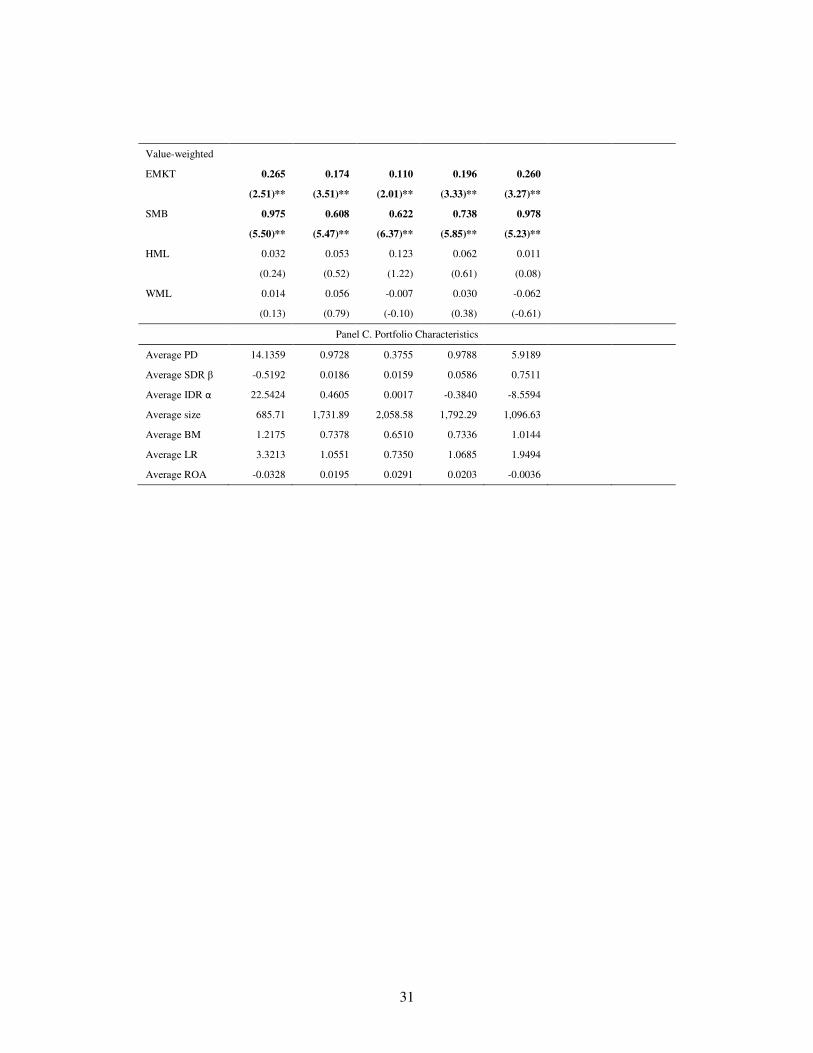
Panel C reports some characteristics of the portfolios. First, SDR betas exhibit large cross-sectional

dispersion, ranging from -0.62 to 0.89, indicating that the effect of aggregate default risk varies substantially

across stocks. In accordance with Barinov (2013), negative SDR betas indicate that these portfolios are

indeed a good hedge against increases in VIX, which justifies their low returns. Second, we find interesting

15 As discussed above, we only report results with the VIX SDR beta as a measure of exposure to aggregate default

risk, but our results are robust if we use the median SDR beta instead. 16 Da and Gao (2010) argue that the high returns of risky stocks are not compensation for SDR, but the result of short-

term return reversal caused by price pressure in the month of portfolio formation. Thus, in accordance with the default

anomaly literature, they find that risky stocks deliver low returns if the second month after portfolio formation is used

instead. To address this critique, we test for return persistence in our SDR beta sorted portfolios. We find no evidence

of return reversal: the return of the highest and lowest SDR beta quintiles differ 8 months before portfolio formation,

the difference is maximized in the portfolio formation month, and persists for almost 8 months after portfolio

formation (even if we assume zero recovery in defaults).

14

non-monotonic patters across the beta portfolios: (a) both high and low SDR beta stocks have higher PDs

than medium SDR beta stocks; (b) they also have higher LRs and lower ROA; (c) they are also, on average,

smaller in size and have higher BM ratios (which is consistent with the results from portfolio sorts on credit

risk premia estimated from CDS spreads by Friewald, Wagner and Zechner, 2013). Therefore the SDR beta

conveys information that is different from that incorporated in other common default risk measures and

stock characteristics. Finally, we find a negative relation between SDR betas and IDR alphas, as the

idiosyncratic component of the PD increases almost monotonically across the SDR beta portfolios. This is

in accordance with Avramov et al. (2013), who document a negative cross-sectional relation between

exposures to systematic and firm-specific risks.

To conclude, the findings in this section show that SDR betas, measured as sensitivities of the physical

PDs to a common aggregate default risk factor (here VIX) are positively related to stock returns and that

high PD stocks can have quite different SDR betas among them.17

C. IDR Alphas and Stock Returns: A negative relation

We now sort stocks based on the IDR alphas.18 Each month, from January 1992 to December 2012, we use

the most recent IDR alpha for each firm and sort the stocks into five portfolios. As before, we adjust monthly

IDR alphas by their country average for this month. Table 7 reports the results.

(TABLE 7)

Panel A shows that the difference in returns between high and low IDR alpha stocks is negative for

both equally and value-weighted returns, as in the case of PDs. It is also significant at a five percent level

for value-weighted returns and CAPM alphas. In Panel B, we see that factor loadings on the market factor

(EMKT) and the size factor (SMB) do not decrease monotonically along the IDR alpha portfolios, but they

17 In unreported results, available upon request, we use double-sorted portfolios to analyze the relation between returns

and SDR betas while controlling for the physical PD. We find that the exposure to aggregate default risk is

significantly rewarded for stocks with low PDs, which are typically stocks less subject to market imperfections. 18 Our results are robust if we measure the idiosyncratic component of default risk as the sum of IDR alphas and

residuals from regression (1).

15

follow the same patterns as for SDR beta portfolios. Specifically, both high and low IDR alpha stocks have

higher loadings than medium IDR alpha stocks. As before, the factor loadings on the value factor (HML)

are not significant. Panel C reports some characteristics of the portfolios. IDR alphas exhibit large cross-

sectional dispersion, ranging from -8.5594 to 22.5424. In accordance with our previous findings on SDR

beta portfolios, both high and low IDR alpha stocks have higher PDs, are smaller, have higher BM and

LRs, and lower ROA than medium IDR alpha stocks. As before, we document a negative relation between

SDR betas and IDR alphas. Therefore, stocks that have low exposures to aggregate default risk are

associated with high firm-specific risks. These results are initial evidence that the default anomaly can be

explained by the non-monotonic relationship between the physical PD and its idiosyncratic component.

IV. Explaining the Default Anomaly

This section sheds more light on the relation between default risk and stock returns. Our main focus is to

understand what the main drivers of the default anomaly are, and therefore we apply a sequential two-sort

procedure to investigate it. Given the results above, we sort on physical PDs while controlling for the

idiosyncratic level of default risk. We use tertiles instead of quintiles to guarantee an adequate number of

stocks in all portfolios. Specifically, each month, we first sort stocks into three portfolios based on their

country-adjusted IDR alpha and, within each IDR alpha portfolio, we further sort stocks in three portfolios,

based on the country-adjusted physical PD. For brevity, we report value-weighted returns but results remain

qualitatively similar for equally-weighted returns. Table 8 reports the results.

(TABLE 8)

Panel A shows the time-series monthly average of the value-weighted returns and alphas, as well as

average monthly returns and alphas for portfolios going long the highest PD tertile and short the lowest PD

tertile of stocks. Interestingly, we find that the default anomaly is significant only for stocks in the highest

IDR alpha tertile, but it is absent in the other two IDR alpha tertiles. Thus, the difference in returns between

16

high and low PD portfolios is negative and significant only when the idiosyncratic component of the PD is

very high. Panel B reports various characteristics of each portfolio. Both stocks in the highest and lowest

IDR alpha tertiles have higher PDs than stocks in the medium IDR alpha tertile. Still, low IDR alpha stocks

have lower PD levels than stocks in the high IDR alpha portfolio. They also differ in terms of their SDR

betas. While stocks in the highest IDR alpha tertile have, on average, negative SDR betas, indicating that

they are a good hedge against aggregate default risk (which explains their low returns), stocks in the lowest

IDR alpha tertile have high SDR betas Another interesting finding is that, in the lowest IDR alpha tertile,

as PD increases, SDR betas rise and IDR alphas fall. This shows that, for stocks with low idiosyncratic risk,

the physical PD is a better proxy to exposures to aggregate default risk. Finally, size and ROA decrease and

BM and LR increase monotonically as PD increases in all three IDR alpha tertiles, indicating that stocks

with high PDs are, on average small, value stocks, with high leverage and low profitability.

Overall, the results above show that the negative relation between physical PD and returns is only

present for stocks with very high firm-specific risk. High IDR alpha stocks have, on average, negative

exposures to aggregate default risk, thus constituting a hedge against bad market conditions. Moreover,

among high IDR alpha stocks, this hedging ability increases as PD increases (i.e. the SDR betas become

more negative). We therefore argue that (1) the so-called “default anomaly” is only found in firms with

high idiosyncratic risk and (2) it is not an “anomaly”, in the sense that the negative returns on the High-

Low PD portfolios are compensated by its hedging ability. On the contrary, for low IDR alpha stocks, the

physical PD is a better measure of the firm’s sensitivity to aggregate default risk; thus, in this case, higher

PD is rewarded with higher returns.

V. Conclusions

In this paper, we shed more light on the recent contradictory literature that studies the relation between

default risk and stock returns. We first follow the Merton model to calculate monthly physical probabilities

of default for individual firms. We then use a novel approach to decompose these estimated PDs into

systematic and idiosyncratic components. Unlike previous studies, our methodology does not require data

17

on bonds or CDS markets. It therefore allows us to carry the analysis for a more comprehensive sample of

European firms, which notably includes micro-cap firms. This heterogeneity is important as previous work

has often associated default risk to other firm characteristics such as size and book-to-market ratios.

Initially, we find evidence consistent with a possible default anomaly, i.e. stocks with high physical

PDs have on average lower returns. However, a closer look shows that the physical PD is usually a poor

measure of exposures to aggregate default risk. Using estimated SDR betas to sort the stocks, we document

a positive and significant relation between default risk and returns. In other words, investors indeed require

a premium to hold stocks that are riskier when aggregate default risk is higher. Therefore it is the

idiosyncratic, not the systematic part, driving the default anomaly. We confirm this conjecture by showing

that stocks sorted on firm-specific risk have on average lower returns. Investors do not require

compensation to hold stocks with high firm-specific risk because these stocks are a source of portfolio

diversification. In fact, we show that stocks with high IDR alphas also have lower (negative) SDR betas. A

double-sort test, where we sort stocks based on their physical PDs after controlling for IDR alphas, finds

that the negative relation between risk and returns is significant only for high IDR alpha stocks.

Our results therefore suggest that riskier stocks, as measured by the physical PDs, will tend to

underperform because they have on average lower exposures to aggregate default risk. Their riskiness is

mostly idiosyncratic and can be diversified away, thus providing an explanation for the default anomaly

typically found in the literature. On the contrary, it is the systematic component of default risk, measured

by the SDR betas, that requires a return premium.

18

References

Altman, Edward I. (1968). “Financial Ratios, Discriminant Analysis and the Prediction of Corporate

Bankruptcy.” The Journal of Finance 23(4), 589-609.

Ang, Andrew, Robert J. Hodrick, Yuhang Xing, and Xiaoyan Zhang. (2006). “The Cross-Section of

Volatility and Expected Returns.” The Journal of Finance 61(1), 259-299.

Anginer, Deniz, and Çelim Yıldızhan. (2013). “Is there a Distress Risk Anomaly? Pricing of Systematic Default Risk in the Cross Section of Equity Returns.” Working Paper.

Aretz, Kevin, Chris Florackis, and Alexandros Kostakis. (2013). “Do Stock Returns Really Decrease with

Default Risk? New International Evidence.” Working paper.

Avramov, Doron, Scott Cederburg, and Satadru Hore. (2011). “Cross-Sectional Asset Pricing Puzzles: A

Long-Run Perspective.” Working Paper.

Avramov, Doron, Tarun Chordia, Gergana Jostova, and Alexander Philipov. (2009). “Credit Ratings and

the Cross-Section of Stock Returns.” Journal of Financial Markets 12(3), 469-499.

Avramov, Doron, Tarun Chordia, Gergana Jostova, and Alexander Philipov. (2013). “Anomalies and

Financial Distress.” Journal of Financial Economics 108(1), 139-159.

Bansal, Ravi, Dana Kiku, Ivan Shaliastovich, and Amir Yaron. (2013). “Volatility, the Macroeconomy, and

Asset Prices.” The Journal of Finance, forthcoming.

Banz, Rolf W. (1981). “The Relationship between Return and Market Value of Common Stocks.” Journal

of Financial Economics 9(1), 3-18.

Barinov, Alexander. (2012). “Aggregate volatility risk: Explaining the small growth anomaly and the new

issues puzzle.” Journal of Corporate Finance 18(4), 763-781.

Bekaert, Geert, Campbell R. Harvey, Christian T. Ludblad, Stephan Siegel. (2013). “The European Union,

the Euro, and Equity Market Integration.” Journal of Financial Economics 109(3), 583-603.

Black, Fischer, and Myron Scholes. (1973). “The Pricing of Options and Corporate Liabilities.” Journal of

Political Economy 81(3), 637-654.

Campbell, John Y., Jens Hilscher, and Jan Szilagyi. (2008). “In Search of Distress Risk.” The Journal of

Finance 63(6), 2899–2939.

Chan, L.K.C., Nai-fu Chen. (1991). “Structural and Return Characteristics of Small and Large Firms. The

Journal of Finance 46(4), 1467-1484.

19

Chan-Lau, J. A. (2006). Is Systematic Default Risk Priced in Equity Returns? A Cross-sectional Analysis

using Credit Derivatives Prices. IMF working paper, 148.

Chava, Sudheer, Amiyatosh Purnanandam. (2010). “Is Default Risk Negatively Related to Stock Returns?”

The Review of Financial Studies 23(6), 2523-2559.

Chen, Long, and Lu Zhang. (2010). “A Better Three-Factor Model That Explains More Anomalies.” The


Collin-Dufresne, Pierre, Robert S. Goldstein, J. Spenser Martin. (2001). “The Determinants of Credit

Spread Changes.” The Journal of Finance 56(6), 2177-2207.

Conrad, Jennifer, Nishad Kapadia, and Yuhang Xing. (2012) “What Explains the Distress Risk Puzzle:

Death or Glory?” Working paper.

Da, Zhi, and Pengjie Gao. (2010). “Clientele Change, Liquidity Shock, and the Return on Financially

Distressed Stocks.” Journal of Financial and Quantitative Analysis 45(1), 27-48.

Dichev, Ilia D. (1998). “Is the Risk of Bankruptcy a Systematic Risk?” The Journal of Finance 53(3), 1131–

1147.

Fama, Eugene F., and Kenneth R. French. (1992). “The Cross-Section of Expected Stock Returns.” The


Fama, Eugene F., and Kenneth R. French. (1996). “Multifactor Explanations of Asset Pricing Anomalies.”

The Journal of Finance 51(1), 55–84.

Fama, Eugene F., and James D. MacBeth. (1973). “Risk, Return, and Equilibrium: Empirical Tests.”

Journal of Political Economy 81(3), 607-636.

Friedwald, Nils, Christian Wagner, and Josef Zechner. (2013). “Credit Risk Premia and Equity Returns.”

The Journal of Finance, forthcoming.

Garlappi, Lorenzo, and Hong Yan. (2011). “Financial Distress and the Cross-Section of Equity-Returns.”

The Journal of Finance 66(3), 789-822.

Garlappi, Lorenzo, Tao Shu, and Hong Yan. (2008). “Default Risk, Shareholder Advantage, and Stock

Returns.” The Review of Financial Studies 21(6), 2743–2778.

Gao, Pengjie, Christopher A. Parsons, and Jainfeng Shen. (2013). “The Global Relation Between Financial

Distress and Equity Returns.” Working paper.

George Thomas J., and Chuan-Yang Hwang. (2010). “A Resolution of the Distress Risk and Leverage

Puzzles in the Cross Section of Stock Returns.” Journal of Financial Economics 96(1), 56-79.

20

Griffin, John M., and Michael L. Lemmon. (2002). “Book-to-Market Equity, Distress Risk and Stock

Returns.” The Journal of Finance 57(5), 2317–2336.

Hilscher, Jens, and Mungo Wilson. (2013). “Credit Ratings and Credit Risk: Is One Measure Enough?”

Working Paper.

Kapadia, Nishad. (2011). “Tracking down Distress Risk.” Journal of Financial Economics 102(1), 167-182.

Kim, Suk Joong, Fariborz Moshirian, Eliza Wu. (2006). “Evolution of International Stock and Bond Market

Integration: Influence of the European Monetary Union.” Journal of Banking and Finance 30(5), 1507-

1534.

Lewellen, Jonathan. (1999). “The Time-Series Relations among Expected Returns, Risk and Book-to-

Market.” Journal of Financial Economics 54(1), 5-43.

Lopez, Jose A. (2004). “The Empirical Relationship between Average Asset Correlation, Firm Probability

of Default, and Asset Size”. Journal of Financial Intermediation 13(2), 263-283.

Merton, Robert C. (1974). “On the Pricing of Corporate Debt: The Risk Structure of Interest Rates.” The


Newey, Whitney K., and Kenneth D. West. (1987). “A Simple, Positive Semi-Definite, Heteroskedasticity

and Autocorrelation Consistent Covariance Matrix.” Econometrica 55(3), 703-708.

Nielsen, Caren Yinxia G. (2013). “Is Default Risk Priced in Equity Returns?” Working Paper.

Ohlson, James A. (1980). “Financial Ratios and the Probabilistic Prediction of Bankruptcy.” Journal of

Accounting Research 18(1), 109‐131.

Ozdagli, Ali K. (2013). “Distressed, but not risky: Reconciling the empirical relationship between financial

distress, market-based risk indicators, and stock returns (and more)”. Working paper.

Pan, Jun, and Kenneth J. Singleton. (2008). “Default and Recovery Implicit in the Term Structure of

Sovereign CDS Spreads.” The Journal of Finance 63(5), 2345–2384.

Schaefer, Stephen M., and Ilya A. Strebulaev. (2008). “Structural Models of Credit Risk are Useful:

Evidence from Hedge Ratios on Corporate Bonds.” Journal of Financial Economics 90(1), 1-19.

Shumway, Tyler, and Vincent A. Warther. (1999). “The Delisting Bias in CRSP’s Nasdaq Data and its

Implications for the Size Effect.” The Journal of Finance 54(6), 2361–2379.

Vassalou, Maria, and Yuhang Xing. (2004). “Default Risk in Equity Returns.” The Journal of Finance

59(2), 831–868.

21

Table 1

Defaulted Firms as a Percentage of Total Firms

The table lists the total number of active firms and delistings due to default for every year

of our sample period. The number of active firms is the average number of firms across

all months of the year. The number of firms that were delisted due to default is hand-

collected data from various public sources.

Year Active Firms Defaults (%)

1990 1,244 1 0.08

1991 1,681 4 0.24

1992 2,072 12 0.58

1993 2,242 6 0.27

1994 2,322 9 0.39

1995 2,374 11 0.46

1996 2,398 14 0.58

1997 2,471 10 0.40

1998 2,526 19 0.75

1999 2,815 20 0.71

2000 2,912 20 0.69

2001 2,985 41 1.37

2002 3,150 41 1.30

2003 3,434 37 1.08

2004 3,548 34 0.96

2005 3,487 39 1.12

2006 3,378 24 0.71

2007 3,406 26 0.76

2008 3,521 83 2.36

2009 3,700 55 1.49

2010 3,906 42 1.08

2011 3,904 39 1.00

2012 3,705 11 0.30

22

Table 2

Characteristics of the Final Sample: Breakdown by Size and Country

This table presents details on the characteristics of our final sample. Panel A shows descriptive statistics for the distribution of firms and

firm-months across size classes. # of firms is the available number of firms for all years for which we are able to calculate monthly

values of the Merton measure. # of firm-months is the number of observations. We provide also the relative fractions of total firms and

firm-months that each size class represents. Finally, the column "Total MC" shows the average total market capitalization of each size

class during the years of the study. We measure market capitalization in millions of euros. Panel B presents the breakdown of firms and

firm-months by country, with corresponding percentages. Start date is the date at which the information on firms of a given country

starts to be available; the end date in our sample, December 2012, is the same for all countries.

Panel A. Breakdown by Size

Segment Size # of firms (%) # of firm-months (%) Total MC (%)

Nano cap < 10 mio 1,419 16.81 106,570 13.22 7,401 0.11

Micro cap < 50 mio 2,631 31.18 219,273 27.20 68,153 1.03

Small cap < 150 mio 1,678 19.88 158,265 19.63 150,178 2.27

Mid cap < 1 bio 1,855 21.98 205,855 25.54 735,025 11.11

Large cap < 50 bio 839 9.94 112,526 13.96 4,239,777 64.07

Mega cap ≥ 50 bio 17 0.20 3,668 0.45 1,417,300 21.42

Overall sample 8,439 806,157 6,617,834

Panel B. Breakdown by Country

Country Start date # of firms (%) # of firm-months (%)

Austria Jan-90 112 1.33 11,676 1.45

Belgium Jan-90 151 1.79 17,842 2.21

Bulgaria Mar-08 130 1.54 4,009 0.50

Czech Republic Mar-98 71 0.84 3,679 0.46

Denmark Jan-90 195 2.31 24,151 3.00

Finland Jan-90 146 1.73 18,589 2.31

France Jan-90 1,126 13.34 111,829 13.87

Germany Jan-90 1,104 13.08 112,428 13.95

Greece Oct-90 315 3.73 35,558 4.41

Hungary Mar-95 45 0.53 3,558 0.44

Ireland Jan-90 68 0.81 8,549 1.06

Italy Jan-90 340 4.03 37,353 4.63

Netherlands Jan-90 213 2.52 28,940 3.59

Norway Jan-90 290 3.44 24,632 3.06

Poland Mar-95 249 2.95 10,620 1.32

Portugal Oct-90 94 1.11 10,002 1.24

Romania Mar-02 65 0.77 2,690 0.33

Serbia Jan-12 47 0.56 445 0.06

Spain Jan-90 175 2.07 22,619 2.81

Sweden Jan-90 525 6.22 42,856 5.32

Switzerland Jan-90 232 2.75 31,695 3.93

United Kingdom Jan-90 2,746 32.54 242,437 30.07

Overall Sample 8,439 100.00 806,157 100.00

23

Table 3

The Merton Measure and Other Firm Characteristics

The table presents descriptive statistics for the average Merton measure, monthly returns, size and BM ratio over the period January 1990 to December 2012. The sample spans 22 European countries. Monthly return is the time-

series average of the cross-sectional average returns within each country. We measure return in euros and express it in percent. Merton measure, size and BM are the time-series averages of the cross-sectional average Merton

measures, market capitalizations and BM ratios. We express the Merton measure in percentage terms (as it is a probability) and market capitalization in millions of euros.

Merton measure Monthly Returns Size BM

Country Mean Median St. Dev. Mean Median St. Dev. Mean Median St. Dev. Mean Median St. Dev.

Austria 4.36 3.08 3.42 0.55 0.58 5.21 541.11 313.22 389.08 0.80 0.78 0.27

Belgium 4.70 3.96 2.88 0.63 0.90 4.16 963.20 889.92 492.07 0.84 0.81 0.18

Bulgaria 14.29 12.99 8.46 -0.64 0.28 8.18 33.02 25.84 22.61 1.74 1.83 0.35

Czech Republic 3.31 1.25 3.87 1.28 1.33 4.38 481.78 505.48 297.82 1.72 1.47 0.68

Denmark 4.09 2.76 3.10 0.69 0.78 4.64 580.10 489.44 337.62 0.90 0.93 0.23

Finland 4.11 2.63 4.63 0.95 0.52 6.22 1,247.22 1,129.59 848.93 0.74 0.69 0.25

France 5.00 4.28 2.53 0.77 0.94 4.63 1,557.86 1,619.24 576.00 0.82 0.81 0.18

Germany 4.67 3.76 3.07 0.55 0.79 3.93 1,457.07 1,443.94 431.23 0.70 0.64 0.23

Greece 6.71 4.61 5.79 1.01 -0.04 10.71 197.65 176.01 137.97 1.12 0.83 0.81

Hungary 9.14 8.76 5.24 1.62 1.15 9.39 82.84 83.77 39.55 1.33 1.33 0.48

Ireland 5.56 4.64 3.13 1.09 1.21 6.48 784.02 799.62 512.20 0.93 0.82 0.35

Italy 6.42 5.72 3.23 0.31 0.22 6.40 1,492.03 1,476.92 930.09 1.00 0.98 0.30

Netherlands 3.42 2.91 2.21 0.58 0.86 4.93 1,832.05 1,866.32 920.79 0.75 0.72 0.21

Norway 7.37 6.85 4.23 1.11 1.43 6.83 508.20 426.60 262.46 0.89 0.86 0.32

Poland 10.27 8.57 9.51 1.31 0.69 10.82 69.94 38.80 58.53 1.27 1.04 0.76

Portugal 7.31 6.69 4.04 0.85 0.20 5.70 659.05 635.25 453.15 1.15 1.11 0.30

Romania 16.69 13.03 10.09 2.02 1.33 9.11 87.34 39.06 87.19 2.15 2.12 0.53

Serbia 12.89 13.26 3.19 0.59 0.45 5.02 17.20 16.96 2.34 3.21 3.19 0.19

Spain 4.16 3.96 2.65 0.68 0.78 5.81 2,142.53 1,995.74 1,246.68 0.89 0.84 0.36

Sweden 6.64 6.21 4.13 1.02 0.91 7.05 1,084.76 886.09 681.68 0.77 0.74 0.28

Switzerland 3.13 2.34 2.41 0.75 0.95 4.54 2,187.33 2,356.76 961.16 0.88 0.83 0.26

United Kingdom 4.27 3.88 2.00 0.81 1.15 5.54 1,288.24 1,367.40 559.96 0.86 0.82 0.23

Overall Sample 5.84 4.44 5.10 0.86 0.82 6.50 1,006.23 765.26 896.78 0.99 0.86 0.50

24

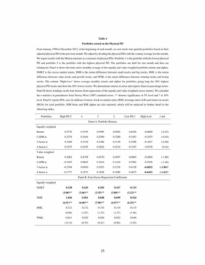
Table 4

Portfolios sorted on the Physical PD

From January 1990 to December 2012, at the beginning of each month, we sort stocks into quintile portfolios based on their

adjusted physical PD in the previous month. We adjust by dividing the physical PDs with the country average for this month.

We report results with the Merton measure as a measure of physical PDs. Portfolio 1 is the portfolio with the lowest physical

PD and portfolio 5 is the portfolio with the highest physical PD. The portfolios are held for one month and then are

rebalanced. Panel A shows the time-series monthly average of the equally and value-weighted portfolio returns and alphas.

EMKT is the excess market return, SMB is the return difference between small stocks and big stocks, HML is the return

difference between value stocks and growth stocks, and WML is the return difference between winning stocks and losing

stocks. The column "High-Low" shows average monthly returns and alphas for portfolios going long the 20% highest

physical PD stocks and short the 20% lowest stocks. We denominate returns in euros and express them in percentage terms.

Panel B shows loadings on the four factors from regressions of the equally and value-weighted excess returns. We calculate

the t-statistics in parentheses from Newey-West (1987) standard errors. ** denotes significance at 5% level and * at 10%

level. Panel C reports PDs, size (in millions of euros), book-to-market ratios (BM), leverage ratios (LR) and return-on-assets

(ROA) for each portfolio. SDR betas and IDR alphas are also reported, which will be analyzed in further detail in the

following tables.

Portfolios High PD 5 4 3 2 Low PD 1 High-Low t-stat

Panel A. Portfolio Returns

Equally-weighted

Return 0.5776 0.5195 0.5985 0.6502 0.6436 -0.0660 (-0.25)

CAPM α 0.2379 0.1644 0.2569 0.3290 0.3453 -0.1075 (-0.44)

3-factor α 0.2269 0.1534 0.2386 0.3130 0.3296 -0.1027 (-0.48)

4-factor α 0.3575 0.2195 0.2922 0.3219 0.3197 0.0378 (0.16)

Value-weighted

Return 0.2062 0.4758 0.4570 0.4597 0.6965 -0.4904 (-1.08)

CAPM α -0.1955 0.0845 0.1014 0.1216 0.3982 -0.5936 (-1.40)

3-factor α -0.2704 0.0450 0.1053 0.1518 0.4128 -0.6832 (-1.84)*

4-factor α -0.1777 0.1973 0.1828 0.1890 0.4675 -0.6452 (-1.63)*

Panel B. Four-Factor Regression Coefficients

Equally-weighted

EMKT 0.238 0.245 0.205 0.167 0.133

(3.00)** (3.66)** (3.35)** (3.08)** (3.12)**

SMB 1.036 0.961 0.848 0.699 0.524

(6.51)** (6.60)** (7.00)** (6.57)** (6.25)**

HML 0.121 0.132 0.143 0.134 0.115

(0.86) (1.07) (1.33) (1.37) (1.46)

WML -0.011 0.025 0.026 0.052 0.049

(-0.14) (0.35) (0.41) (0.86) (1.02)

25

Value-weighted

EMKT 0.286 0.296 0.248 0.177 0.090

(3.28)** (3.56)** (2.91)** (2.52)** (2.09)**

SMB 1.345 1.175 1.001 0.716 0.451

(6.79)** (6.65)** (6.69)** (5.55)** (5.24)**

HML 0.336 0.204 0.088 0.005 0.013

(1.83) (1.31) (0.62) -0.05 -0.15

WML 0.016 -0.034 0.008 0.035 0.021

-0.14 (-0.35) (0.09) (0.43) (0.31)

Panel C. Portfolio Characteristics

Average PD 22.5600 1.7749 0.1614 0.0096 0.0000

Average Size 286.42 530.43 1,000.41 1,707.40 2,674.78

Average BM 1.4545 1.0046 0.7706 0.6097 0.4949

Average LR 4.0889 1.7436 1.0925 0.7103 0.4025

Average ROA -0.0623 -0.0045 0.0177 0.0297 0.0369

Average SDR β 0.0590 0.1574 0.0770 0.0327 0.0060

Average IDR α 14.3208 0.7767 -0.0892 -0.0567 0.1510

26

Table 5

Summary Statistics on VIX

In this table, VIX is the CBOE volatility index and ∆mVIX is the monthly change in VIX. Mean, Std, Skew, and Kurt refer to

the mean, standard deviation, skewness, and kurtosis, respectively. VSTOXX, VFTSE and VDAX are the EUROSTOXX 50,

FTSE 100 and DAX volatility indices, which follow the VIX methodology for the European, UK, and German markets

respectively. ∆mEurostoxx50 is the monthly change in EUROSTOXX 50 and ∆mMSCIEurope is the monthly change in MSCI

Europe. EMKT is the value-weighted excess return on the European market portfolio over the risk-free rate and SMB and HML

are the Fama-French factors for Europe. Aggregate PD is the monthly average and Median PD is the monthly median of the

Merton measure values of all firms. We calculate the t-statistics from Newey-West (1987) standard errors (up to five lags).

Panel A. Summary Statistics on VIX and VIX Monthly Changes (∆mVIX)

Mean Std Skew Kurt

VIX 20.1978 8.0533 2.0133 10.1303

∆mVIX -0.0267 4.2391 0.8229 8.1017

Panel B. Correlation between VIX and Other Volatility Indices

VSTOXX VFTSE VDAX

VIX 0.9100 0.9449 0.9492

Panel C. Correlation between ∆mVIX and European Stock Indices

∆mEUROSTOXX50 ∆mMSCIEurope

∆mVIX -0.6335 -0.5835

Panel D. Correlation between ∆mVIX and Other Factors

EMKT SMB HML

∆mVIX -0.1743 -0.1670 -0.0623

Panel E. Time-Series Regression of the Aggregate and Median Merton measure on VIX

Constant VIX R-squared

Aggregate PD 1.8060 0.1534 0.2686

(5.43) (10.07) Median PD -0.4676 0.0026 0.3112

(-8.30) (11.17)

27

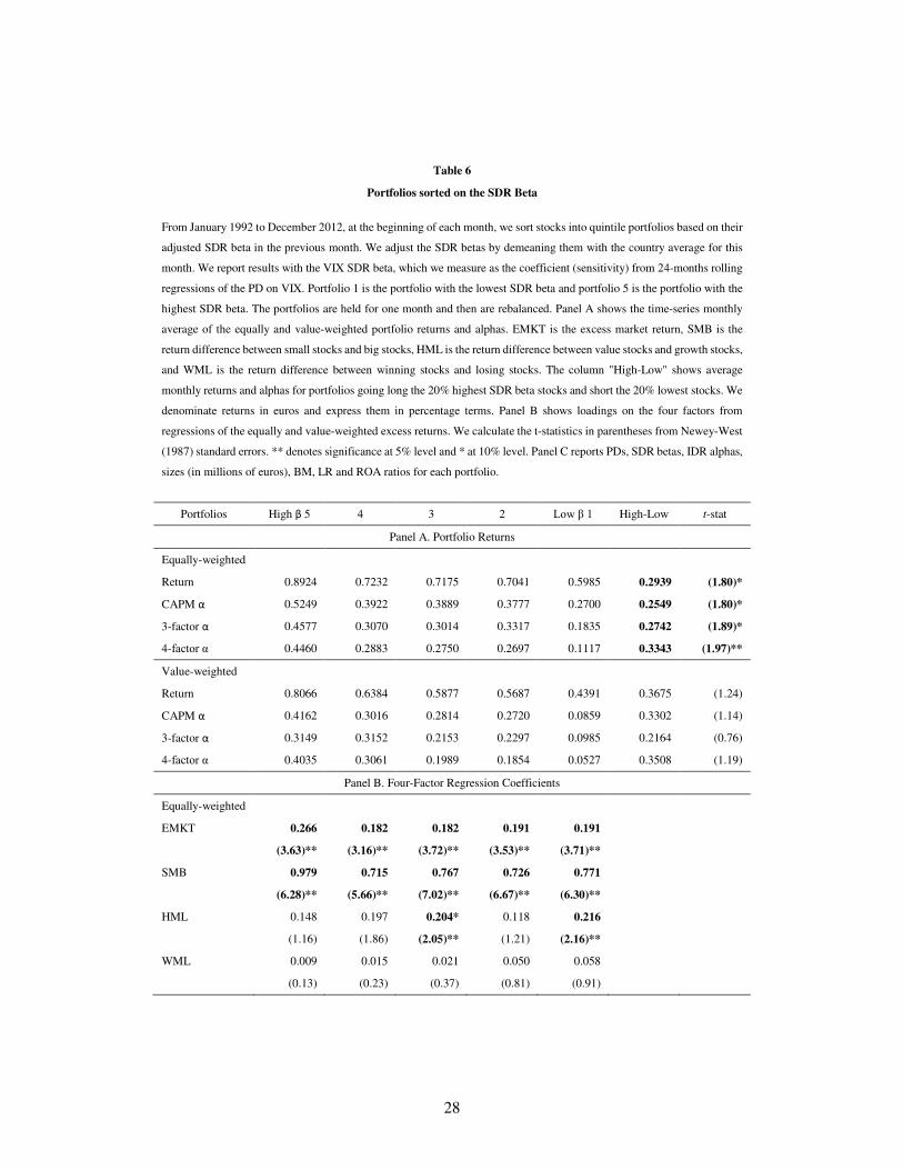
Table 6

Portfolios sorted on the SDR Beta


adjusted SDR beta in the previous month. We adjust the SDR betas by demeaning them with the country average for this

month. We report results with the VIX SDR beta, which we measure as the coefficient (sensitivity) from 24-months rolling

regressions of the PD on VIX. Portfolio 1 is the portfolio with the lowest SDR beta and portfolio 5 is the portfolio with the

highest SDR beta. The portfolios are held for one month and then are rebalanced. Panel A shows the time-series monthly

average of the equally and value-weighted portfolio returns and alphas. EMKT is the excess market return, SMB is the

return difference between small stocks and big stocks, HML is the return difference between value stocks and growth stocks,

and WML is the return difference between winning stocks and losing stocks. The column "High-Low" shows average

monthly returns and alphas for portfolios going long the 20% highest SDR beta stocks and short the 20% lowest stocks. We

denominate returns in euros and express them in percentage terms. Panel B shows loadings on the four factors from

regressions of the equally and value-weighted excess returns. We calculate the t-statistics in parentheses from Newey-West

(1987) standard errors. ** denotes significance at 5% level and * at 10% level. Panel C reports PDs, SDR betas, IDR alphas,

sizes (in millions of euros), BM, LR and ROA ratios for each portfolio.

Portfolios High β 5 4 3 2 Low β 1 High-Low t-stat


Equally-weighted

Return 0.8924 0.7232 0.7175 0.7041 0.5985 0.2939 (1.80)*

CAPM α 0.5249 0.3922 0.3889 0.3777 0.2700 0.2549 (1.80)*

3-factor α 0.4577 0.3070 0.3014 0.3317 0.1835 0.2742 (1.89)*

4-factor α 0.4460 0.2883 0.2750 0.2697 0.1117 0.3343 (1.97)**

Value-weighted

Return 0.8066 0.6384 0.5877 0.5687 0.4391 0.3675 (1.24)

CAPM α 0.4162 0.3016 0.2814 0.2720 0.0859 0.3302 (1.14)

3-factor α 0.3149 0.3152 0.2153 0.2297 0.0985 0.2164 (0.76)

4-factor α 0.4035 0.3061 0.1989 0.1854 0.0527 0.3508 (1.19)


Equally-weighted

EMKT 0.266 0.182 0.182 0.191 0.191

(3.63)** (3.16)** (3.72)** (3.53)** (3.71)**

SMB 0.979 0.715 0.767 0.726 0.771

(6.28)** (5.66)** (7.02)** (6.67)** (6.30)**

HML 0.148 0.197 0.204* 0.118 0.216

(1.16) (1.86) (2.05)** (1.21) (2.16)**

WML 0.009 0.015 0.021 0.050 0.058

(0.13) (0.23) (0.37) (0.81) (0.91)

28

Value-weighted

EMKT 0.287 0.214 0.137 0.133 0.250

(3.60)** (3.82)** (2.54)** (2.45)** (2.38)**

SMB 1.060 0.763 0.652 0.683 0.770

(5.68)** (5.04)** (6.28)** (6.81)** (4.55)**

HML 0.196 -0.040 0.152 0.104 -0.026

(1.37) (-0.36) (1.47) (1.08) (-0.19)

WML -0.071 0.007 0.013 0.036 0.037

(-0.72) (0.09) (0.17) (0.47) (0.43)


Average PD 10.7144 1.6788 0.5810 0.6172 8.7870

Average SDR β 0.8881 0.0516 0.0081 -0.0025 -0.6166

Average IDR α -5.9819 0.3573 0.3122 0.5973 18.7048

Average size 708.81 1,691.08 1,957.37 1,964.43 1,044.72

Average BM 1.1773 0.7985 0.6703 0.6806 1.0280

Average LR 2.8791 1.2538 0.8418 0.8740 2.2675

Average ROA -0.0251 0.0144 0.0272 0.0256 -0.0093

29

Table 7

Portfolios sorted on the IDR Alpha


adjusted IDR alpha in the previous month. We adjust the IDR alphas by demeaning them with the country average for this

month. We report results with the IDR alpha, which we measure as the constant from 24-months rolling regressions of the

PD on VIX. Portfolio 1 is the portfolio with the lowest IDR alpha and portfolio 5 is the portfolio with the highest IDR alpha.

The portfolios are held for one month and then are rebalanced. Panel A shows the time-series monthly average of the equally

and value-weighted portfolio returns and alphas. EMKT is the excess market return, SMB is the return difference between

small stocks and big stocks, HML is the return difference between value stocks and growth stocks, and WML is the return

difference between winning stocks and losing stocks. The column "High-Low" shows average monthly returns and alphas

for portfolios going long the 20% highest IDR alpha stocks and short the 20% lowest stocks. We denominate returns in

euros and express them in percentage terms. Panel B shows loadings on the four factors from regressions of the equally and

value-weighted excess returns. We calculate the t-statistics in parentheses from Newey-West (1987) standard errors. **

denotes significance at 5% level and * at 10% level. Panel C reports PDs, SDR betas, IDR alphas, sizes (in millions of

euros), BM, LR and ROA ratios for each portfolio.

Portfolios High α 5 4 3 2 Low α 1 High-Low t-stat


Equally-weighted

Return 0.6686 0.5484 0.7229 0.8372 0.8545 -0.1858 (-1.17)

CAPM α 0.3437 0.2203 0.3940 0.5016 0.4904 -0.1467 (-1.04)

3-factor α 0.2648 0.1605 0.3193 0.4281 0.4049 -0.1401 (-0.93)

4-factor α 0.1907 0.0888 0.2933 0.3885 0.4263 -0.2357 (-1.32)

Value-weighted

Return 0.4450 0.4243 0.5613 0.6981 0.9573 -0.5124 (-1.97)**

CAPM α 0.0847 0.1073 0.2678 0.3691 0.5894 -0.5046 (-2.00)**

3-factor α 0.0675 0.0905 0.2106 0.3434 0.5682 -0.5007 (-1.86)*

4-factor α 0.0504 0.0209 0.2197 0.3058 0.6456 -0.5952 (-1.81)*


Equally-weighted

EMKT 0.192 0.192 0.184 0.199 0.245

(3.53)** (4.10)** (3.25)** (3.65)** (3.35)**

SMB 0.851 0.706 0.740 0.756 0.903

(6.40)** (5.95)** (6.73)** (6.60)** (6.18)**

HML 0.198 0.154 0.174 0.175 0.182

(1.93) (1.68) (1.69) (1.69) (1.42)

WML 0.060 0.058 0.021 0.032 -0.017

(0.88) (1.02) (0.32) (0.52) (-0.24)

30

Value-weighted

EMKT 0.265 0.174 0.110 0.196 0.260

(2.51)** (3.51)** (2.01)** (3.33)** (3.27)**

SMB 0.975 0.608 0.622 0.738 0.978

(5.50)** (5.47)** (6.37)** (5.85)** (5.23)**

HML 0.032 0.053 0.123 0.062 0.011

(0.24) (0.52) (1.22) (0.61) (0.08)

WML 0.014 0.056 -0.007 0.030 -0.062

(0.13) (0.79) (-0.10) (0.38) (-0.61)


Average PD 14.1359 0.9728 0.3755 0.9788 5.9189

Average SDR β -0.5192 0.0186 0.0159 0.0586 0.7511

Average IDR α 22.5424 0.4605 0.0017 -0.3840 -8.5594

Average size 685.71 1,731.89 2,058.58 1,792.29 1,096.63

Average BM 1.2175 0.7378 0.6510 0.7336 1.0144

Average LR 3.3213 1.0551 0.7350 1.0685 1.9494

Average ROA -0.0328 0.0195 0.0291 0.0203 -0.0036

31

Table 8

Portfolios sorted on the Physical PD controlled by the IDR alpha

From January 1992 to December 2012, at the beginning of each month, we sort stocks into three portfolios based

on their IDR alpha in the previous month. Within each portfolio, we further sort the stocks into three portfolios,

based on their past month's PD. We adjust both IDR alphas and PDs by the country average for this month. The

sequential two-sort procedure produces 9 portfolios in total. The portfolios are held for one month and then are

rebalanced. Panels A shows the time-series monthly average of the value-weighted returns, respectively, for the 9

portfolios as well as average monthly returns and alphas for portfolios going long the 1/3 highest PD stocks and

short the 1/3 lowest PD stocks for all three IDR alpha tertiles. We denominate returns in euros and express them in

percentage terms. We calculate t-statistics in parentheses from Newey-West (1987) standard errors. ** denotes

significance at 5% level and * at 10% level. Panel B reports PDs, SDR betas, IDR alphas, sizes (in millions of

euros), BM, LR and ROA ratios for each portfolio.

High PD Medium PD Low PD High-Low t-stat


Return

High -0.1105 0.2944 0.6686 -0.7791 (-1.90)*

Medium 0.6117 0.4217 0.6185 -0.0068 (-0.03)

Low 0.8658 0.8218 0.8121 0.0537 (0.15)

CAPM α

High -0.4474 -0.0749 0.3600 -0.8074 (-2.03)**

Medium 0.2514 0.1110 0.3369 -0.0855 (-0.34)

Low 0.4839 0.4371 0.4807 0.0032 (0.01)

3-factor α

High -0.5367 -0.2476 0.3854 -0.9221 (-2.45)**

Medium 0.1781 0.0852 0.3037 -0.1256 (-0.61)

Low 0.3494 0.3890 0.4682 -0.1188 (-0.43)

4-factor α High -0.6182 -0.3495 0.3408 -0.9591 (-2.36)**

Medium 0.2728 0.0637 0.2931 -0.0204 (-0.08)

Low 0.3286 0.4680 0.4682 -0.1397 (-0.51)

Panel B. Portfolio Characteristics

Average Probability of Default High α 24.7076 2.0970 0.0269 Medium α 1.4230 0.0179 0.0002 Low α 10.9104 0.9728 0.1867

Average SDR Beta

High α -0.6487 -0.1936 -0.0710 Medium α 0.0488 0.0079 0.0017 Low α 1.0079 0.2979 0.1347

Average IDR Alpha

High α 30.4494 8.2601 2.6320 Medium α 0.0790 -0.0522 -0.0042 Low α -10.3704 -3.8171 -1.8405

Average Size

High α 304.65 695.78 2,305.09 Medium α 869.65 1,964.63 3,044.43 Low α 525.11 1,205.18 2,337.58

32

Average Book-to-Market

High α 1.4969 0.9854 0.6060 Medium α 0.8975 0.6193 0.4949 Low α 1.2925 0.8516 0.5959

Average Leverage Ratio

High α 4.7897 1.8378 0.7441 Medium α 1.3513 0.6996 0.3793 Low α 2.8937 1.3207 0.6827

Average Return-on-Assets High α -0.0606 -0.0063 0.0274 Medium α 0.0104 0.0318 0.0392 Low α -0.0303 0.0138 0.0315

33

Panel A

Panel B

Figure 1. Merton measure, Campbell, Hilscher and Szilagyi Measure and Volatility Index. The figure plots the monthly

aggregate Merton (left scale) and CHS (right scale) measures for firms in the overall sample (Panel A) and the monthly aggregate

Merton measure (left scale) and monthly VIX (right scale) values (Panel B). We define the aggregate Merton and CHS measures

as simple averages of the values of all firms. The Merton measure is the PD estimated following Vassalou and Xing (2002), which

we calculate from the Merton's model. The CHS measure is the one used in Campbell, Hilscher and Szilagyi (2008), which we

calculate from a dynamic logit model using historical defaults. VIX is available daily from the CBOE and represents a measure of

expected stock market volatility. The columns denote recession periods in the Euro area, as indicated by OECD.

0.000

0.000

0.001

0.001

0.001

0.001

0.001

0.002

0.002

0.00

0.02

0.04

0.06

0.08

0.10

0.12Ja

n-9

0

Dec

-90

No

v-9

1

Oct

-92

Sep

-93

Au

g-9

4

Jul-

95

Jun-9

6

May

-97

Ap

r-98

Mar

-99

Feb

-00

Jan

-01

Dec

-01

No

v-0

2

Oct

-03

Sep

-04

Au

g-0

5

Jul-

06

Jun-0

7

May

-08

Ap

r-09

Mar

-10

Feb

-11

Jan

-12

Dec

-12

CH

S m

easu

re

Mer

ton

mea

sure

Correlation = 0.92

Merton measure CHS Measure

0.00

10.00

20.00

30.00

40.00

50.00

60.00

0.00

0.02

0.04

0.06

0.08

0.10

0.12

Jan

-90

Dec

-90

No

v-9

1

Oct

-92

Sep

-93

Au

g-9

4

Jul-

95

Jun-9

6

May

-97

Ap

r-98

Mar

-99

Feb

-00

Jan

-01

Dec

-01

No

v-0

2

Oct

-03

Sep

-04

Au

g-0

5

Jul-

06

Jun-0

7

May

-08

Ap

r-09

Mar

-10

Feb

-11

Jan

-12

Dec

-12

VIX

Mer

ton

mea

sure

Correlation = 0.52

Merton measure VIX

34

Appendix A. The Merton Measure

A.I. Calculating the Physical PDs

Following Vassalou and Xing (2004), we allow only equity and debt in the capital structure of the firm. In

Merton’s model, equity can be viewed as a call option on firm’s assets with a strike price equal to the value

of debt. The reason is that equity is a residual claim, i.e. equity holders lay claim to all cash flows left over

only after debt holders have been satisfied.

The market value of firm’s assets follow a geometric Brownian motion as below: 𝑑𝑑𝑑𝑑𝐴𝐴 = 𝜇𝜇𝑑𝑑𝐴𝐴𝑑𝑑𝑡𝑡 + 𝜎𝜎𝐴𝐴𝑑𝑑𝐴𝐴𝑑𝑑𝑑𝑑, (1)

where 𝑑𝑑𝐴𝐴 is the market value of firm’s assets, with an instantaneous drift 𝜇𝜇, and instantaneous volatility 𝜎𝜎𝐴𝐴. 𝑑𝑑 is a standard Wiener process.

The market value of firm’s equity is given by the Black and Scholes (1973) formula for call options: 𝑑𝑑𝐸𝐸 = 𝑑𝑑𝐴𝐴𝑁𝑁(𝑑𝑑1) − 𝑋𝑋𝑋𝑋−𝑟𝑟𝑟𝑟𝑁𝑁(𝑑𝑑2), (2)

𝑑𝑑1 =ln�𝑉𝑉𝐴𝐴𝑋𝑋 �+�𝑟𝑟+𝜎𝜎𝐴𝐴22 �𝑟𝑟𝜎𝜎𝐴𝐴√𝑟𝑟 , 𝑑𝑑2 = 𝑑𝑑1 − 𝜎𝜎𝐴𝐴√𝑇𝑇, (3)

where 𝑑𝑑𝐸𝐸 is the market value of firm’s equity, 𝑋𝑋 is the book value of debt that has a maturity equal to 𝑇𝑇, 𝑟𝑟

is the risk-free rate, and 𝑁𝑁 is the cumulative density function of the standard normal distribution.

First, we calculate the volatility of equity 𝜎𝜎𝐸𝐸 from daily data of the past 12 months and use it as the

initial value for the estimation of 𝜎𝜎𝐴𝐴. Then, from (2) and (3), we compute 𝑑𝑑𝐴𝐴 for each trading day of the past

12 months using 𝑑𝑑𝐸𝐸 of that day and 𝑋𝑋.19 From the daily values of 𝑑𝑑𝐴𝐴 we calculate 𝜎𝜎𝐴𝐴 for the next iteration.

We repeat this process until the values of 𝜎𝜎𝐴𝐴 from two consecutive observations converge. Once we obtain

19 As Vassalou and Xing (2004) and KMV do, we use current liabilities (WC03101) plus half the long-term debt

(WC03251) to calculate the book value of debt 𝑋𝑋. Also, to account for reporting delays that may influence data

availability, we use the book value of debt at the fiscal year end, only after 4 months have passed from the fiscal year

end.

35

a converged value of 𝜎𝜎𝐴𝐴, we use it to find 𝑑𝑑𝐴𝐴 from (2) and (3). We repeat the process at the end of every

month and obtain monthly values for 𝜎𝜎𝐴𝐴. We use the 1-year T-bill rate at the end of the month as the risk-

free rate. Once we obtain daily values of 𝑑𝑑𝐴𝐴, we compute the drift 𝜇𝜇 as the mean of the change in ln𝑑𝑑𝐴𝐴.

Finally, using the normal distribution implied by Merton, we can show that the theoretical PD at time 𝑡𝑡 is

given by the following formula:

𝑃𝑃𝑃𝑃𝑡𝑡 = 𝑁𝑁(−𝑃𝑃𝑖𝑖𝐷𝐷𝑡𝑡𝐷𝐷𝐷𝐷𝐷𝐷𝑋𝑋 𝑡𝑡𝑡𝑡 𝑃𝑃𝑋𝑋𝐷𝐷𝐷𝐷𝐷𝐷𝐷𝐷𝑡𝑡𝑡𝑡) = 𝑁𝑁(− ln�𝑉𝑉𝐴𝐴,𝑡𝑡𝑋𝑋𝑡𝑡 �+�𝜇𝜇−𝜎𝜎𝐴𝐴22 �𝑟𝑟𝜎𝜎𝐴𝐴√𝑟𝑟 , (4)

where we refer to 𝑃𝑃𝑃𝑃𝑡𝑡 as the Merton measure.

A.II. Evaluating the Performance of the Merton Measure

In order to evaluate the performance of the Merton measure, we employ two widely used measures, the

Hosmer and Lemeshow grouping and the area under the Receiver Operating Characteristic (ROC) curve.

First, based on the Hosmer and Lemeshow method, each month we rank the estimated PDs and divide

them into deciles. Out of the ten groups created (each one containing 1/10 of the firms in that month), the

first group has the smallest average estimated PD and the last the largest. Next, we aggregate the number

of defaulted firms in each decile for each month over the sample period and calculate the corresponding

percentages of the defaulted firms in each decile. The percentage of defaulted firms in the last decile is

58.72. When we look at the last three deciles, this percentage becomes 79.87. This provides us initial

evidence that the Merton measure captures important default-related information.

Second, we construct the area under the ROC curve (AUC) from the estimated PDs versus the actual

status of the firms in each month for all possible cut-off probability values. Specifically, the curve plots the

ratio of correctly classified defaulted firms to actual defaulted firms (sensitivity) and the ratio of wrongly

classified healthy firms to actual healthy firms (1 - specificity) for all possible cut-offs. The AUC ranges

36

from zero to one. A model with an AUC close to 0.5 is considered a random model with no discriminatory

power. An AUC of 0.7 to 0.8 represents good discriminatory power, an AUC of 0.8 to 0.9 very good

discriminatory power and an AUC over 0.9 is exceptional and extremely unusual. The AUC that we obtain

is equal to 0.8212. This result further supports our belief that the Merton measure is indeed a good default

predictor.

As a supplementary and final test, we follow Vassalou and Xing (2004) and compare the PDs of the

defaulted firms (treatment group) with the PDs of a group of non-defaulted firms (control group). For each

defaulted firm, we choose a healthy firm of similar size (market capitalization) and same industry (4-digit

ICB code). We try to match the size of defaulted and healthy firms on the exact month or year of delisting

due to default whenever possible. Figure A1 shows the average PDs of both groups up to 160 months before

delisting. It is apparent that the PDs of both groups move closely together up to four years (48 months)

before delisting. In the beginning of the fourth year before delisting though, the average PD of the treatment

group goes up sharply, whereas the average PD of the control group does not follow this extreme behavior.

Its moderate upward movement can be attributed to general worsening economic conditions in times of

many defaults that move upward all PDs in the economy. The average PD at 𝑡𝑡 = 0 is 0.14 for healthy firms

and 0.34 for defaulted firms (around 1.5 times higher). This final test provides additional support that the

Merton measure captures default risk successfully.

37

Figure A1. Average Merton Measure of treatment group (defaulted firms) and control group (healthy firms). We choose

firms in the control group that have similar size (market capitalization) and same four-digit industry code as those in the treatment

group. Specifically for size, we select firms that have similar size with their defaulted counterparts immediately before they delist.

We also match the month or year of delisting whenever possible.

0.00

0.05

0.10

0.15

0.20

0.25

0.30

0.35

160

155

150

145

140

135

130

125

120

115

110

105

100

95

90

85

80

75

70

65

60

55

50

45

40

35

30

25

20

15

10 5 0

Mer

ton

mea

sure

Months before delisting

Control Group Treatment Group

38

Appendix B. Calculation of the CHS Measure

Following Campbell, Hilscher and Szilagyi (2008), we use eight variables to calculate the CHS measure

(all converted in euros). NIMTA is the ratio of net income (WC07250) to the market-adjusted version of

total assets, where the latter is the sum of the market value of equity and the book value of liabilities

(WC03351); TLMTA is the ratio of total liabilities to the market-adjusted version of total assets; EXRET

is the monthly log excess return relative to the MSCI index of the country that is the firm’s main market;20

SIGMA is the standard deviation of the daily returns over the previous year; RSIZE is the log ratio of firm’s

market value to the total market value of firms in the same country and month; CASHMTA is the ratio of

cash and short-term investments (WC02001) to the market-adjusted version of total assets; MB is the

market-to-book ratio; and PRICE is the log price truncated at the first and third quartiles of the pooled price

distribution. We truncate all other variables at the first and ninety-ninth percentile of their pooled

distributions. We lag all accounting data by at least 4 months and market data by 1 month, to ensure their

availability at the time of default prediction. To avoid excluding firms shortly before they default, we use

data for up to 12 months if more recent data are unavailable.

Table B1 presents summary statistics of these variables. A comparison of Panels B and C reveals the

differences of defaulted observations. They have lower profitability, higher leverage, lower stock excess

returns, higher stock volatility, lower MB ratios and lower prices compared to healthy observations. They

are also smaller. Finally, contrary to the findings of Campbell et al. (2008) for the US, but in accordance

with Aretz, Florackis and Kostakis (2013) for Europe, they hold on average more cash.

Concerning the applied estimation method, we assume that the marginal probability of default over the

next period follows a logistic distribution and is given by:

20 Robustness checks using other indices yield same results.

39

𝑃𝑃𝑃𝑃(𝑌𝑌𝑖𝑖,𝑡𝑡 = 1|𝑥𝑥𝑖𝑖,𝑡𝑡−1) =11+ exp�−α −𝛽𝛽𝑥𝑥𝑖𝑖,𝑡𝑡−1�, (5)

where 𝑌𝑌𝑖𝑖,𝑡𝑡 is an indicator that equals one if the firm defaults in period 𝑡𝑡 and zero otherwise, i.e. if the firm

disappears from the sample for some reason other than default, such as delisting due to a merger; and 𝛽𝛽𝑥𝑥𝑖𝑖,𝑡𝑡−1 is a function of firm-specific characteristics that includes a vector of predictor variables 𝑥𝑥𝑖𝑖,𝑡𝑡−1

known at the end of the previous period. Finally, to capture cross-country differences, we follow two

different methods: (i) we estimate separate models for each country; (ii) we introduce country fixed effects

and estimate only one model.

Table B2 reports the regression results only under method (ii) due to space limitations. The coefficients

confirm the findings from Table C1. The CHS measure is negatively related to profitability (NIMTA),

excess return (EXRET), size (RSIZE), and PRICE. It is positively related to leverage (TLMTA), volatility

(SIGMA), liquidity (CASHMTA) and MB. Most coefficients are significant at a 5% level, with the

exception of CASHMTA and MB. The pseudo-R2 (McFadden’s R2) is 17.4%, indicating a rather good

fit. The pseudo-R2 may look low when compared to R2 values of linear regression models, but such

low values are normal in logistic regression.

40

Table B1

Summary Statistics for the CHS Measure

The table reports summary statistics for all of the accounting and market variables used to calculate the CHS measure. NIMTA is the ratio

of net income (WC07250) to the market-adjusted version of total assets, where the latter is the sum of the market value of equity and the book

value of liabilities (WC03351); TLMTA is the ratio of total liabilities to the market-adjusted version of total assets; EXRET is the monthly log

excess return relative to the MSCI index of the country that is the firm’s main market; RSIZE is the log ratio of firm’s market value to the total

market value of firms in the same country and month; SIGMA is the standard deviation of the daily returns over the previous year; CASHMTA

is the ratio of cash and short-term investments (WC02001) to the market-adjusted version of total assets; MB is the market-to-book ratio; and

PRICE is the log price truncated at the first and third quartiles of the pooled price distribution. All other variables are truncated at the first and

ninety-ninth percentile of their pooled distributions. Panel A describes the distributions of the variables in all observations, Panel B describes

the sample of healthy observations, and Panel C describes the defaulted observations.

NIMTA TLMTA EXRET RSIZE SIGMA CASHMTA MB PRICE

Panel A. All

Mean 0.01 0.45 0.00 -7.98 0.41 0.09 2.33 1.65

Median 0.03 0.44 -0.01 -8.04 0.36 0.06 1.63 1.62

Std.Dev. 0.06 0.23 0.10 2.41 0.20 0.09 2.03 1.03

Min -0.16 0.07 -0.19 -12.01 0.15 0.00 0.40 0.39

Max 0.09 0.84 0.19 -3.61 0.91 0.33 8.22 2.92

N 761,779 761,897 796,573 803,106 803,106 761,578 802,965 803,106

Panel B. Healthy

Mean 0.01 0.45 0.00 -7.98 0.41 0.09 2.33 1.65

Median 0.06 0.23 0.10 2.41 0.20 0.09 2.03 1.03

Std.Dev. 0.03 0.44 -0.01 -8.04 0.36 0.06 1.63 1.62

N 761,257 761,374 795,979 802,511 802,511 761,055 802,370 802,511

Panel C. Defaulted

Mean -0.07 0.64 -0.05 -10.56 0.66 0.10 1.48 0.74

Median 0.09 0.25 0.13 1.88 0.24 0.11 1.90 0.74

Std.Dev. -0.08 0.77 -0.04 -11.39 0.71 0.05 0.69 0.39

N 522 523 594 595 595 523 595 595

41

Table B2

Regression Results for the CHS Measure

The table reports results from the multi-period logit regression of the default indicator on the eight

predictor variables. NIMTA is the ratio of net income (WC07250) to the market-adjusted version of total

assets, where the latter is the sum of the market value of equity and the book value of liabilities

(WC03351); TLMTA is the ratio of total liabilities to the market-adjusted version of total assets; EXRET

is the monthly log excess return relative to the MSCI index of the country that is the firm’s main market;

RSIZE is the log ratio of firm’s market value to the total market value of firms in the same country and

month; SIGMA is the standard deviation of the daily returns over the previous year; CASHMTA is the

ratio of cash and short-term investments (WC02001) to the market-adjusted version of total assets; MB is

the market-to-book ratio; and PRICE is the log price truncated at the first and third quartiles of the pooled

price distribution. We truncate all other variables at the first and ninety-ninth percentile of their pooled

distributions. We lag all accounting data by at least 4 months and market data by 1 month. The model is

estimated for January 1990 to December 2012, with yearly observations. Parameter estimates are given

first followed by chi-square values in parentheses. Standard errors are cluster-robust to correct for

dependence between firm-year observations of the same firm. Numbers significant at the 5% level are in

bold.

NIMTA -4.449 (-7.15)

TLMTA 2.914 (11.33)

EXRET -1.550 (-3.91)

RSIZE -0.455 (-10.29)

SIGMA 2.311 (9.19)

CASHMTA 0.367 (0.75)

MB 0.014 (0.51)

PRICE -0.253 (-3.32)

Constant -14.160 (-27.54)

Firm-year observations 755,243

Firms 7,980

Distressed firms 522

Country fixed effects Yes

Pseudo R-squared 0.174

Log likelihood -3568.9

Wald test 970.0

42

Documents

Pricing Default Risk: The Good, The Bad, and The Anomaly