Pricing Multi-Name Default Swaps with Counterparty … Brothers | Quantitative Credit Research Pricing Multi-Name Default Swaps with Counterparty Risk 19 November 2003 2 Both our main

Pricing Multi-Name Default Swaps withCounterparty Risk

We present a simple methodology for pricing counterparty risk in multi-name default swaps. In an application to

portfolio loss tranches, we show how fair spreads change as we vary a number of relevant parameters. We also

show that allowing for the possibility of default of the protection seller has a much more significant impact on

fair spreads than allowing for the possibility of default of the protection buyer, other things being equal.

Roy Mashal and Marco Naldi

Fixed IncomeQuantitative Credit Research

November 2003

Lehman Brothers | Quantitative Credit Research Pricing Multi-Name Default Swaps with Counterparty Risk

19 November 2003 1

Pricing Multi-Name Default Swaps with Counterparty Risk1

We present a simple and general methodology for pricing counterparty risk in multi-name default swaps, such as nth-to-default baskets and portfolio loss tranches. The main purpose of our analysis is to derive pricing results without running into the problem of nested valuations, ie, without having to explicitly compute the mark-to-market of the swap in each state where the counterparty defaults. Although the proposed methodology can be used in conjunction with any underlying default model (structural, reduced-form, hybrid), we provide explicit pricing examples for loss tranches of different seniorities by means of a simple and computationally efficient time-to-default simulation, where default dependencies among the reference names and the default-risky counterparty are generated by an appropriately calibrated copula function. We show how fair tranche spreads vary as functions of a) the market-implied default probability of the risky counterparty, b) the asymmetry of the mark-to-market recovery at default, and c) the dependence between the default time of the risky counterparty and the default times of the credits referenced by the swap. Finally, we use our methodology to show that allowing for the possibility of default of the protection seller has a much more significant impact on fair spreads than allowing for the possibility of default of the protection buyer, other things being equal.

1. INTRODUCTION

When an agent enters into an unfunded swap with a default-risky counterparty, she should consider the possibility of her counterparty defaulting before the maturity of the contract. In this case, some or all of the contractual obligations will be left unfulfilled, and she may incur a mark-to-market loss. Examples of such situations are:

• A first-to-default protection buyer defaulting before maturity and before the default of the reference name.

• A tranche protection seller defaulting before maturity and before the notional of his exposure is completely eroded by defaults of the reference names.

We present a simple and general methodology for pricing counterparty risk in multi-name default swaps, such as nth-to-default baskets and portfolio loss tranches. The main purpose of our analysis is to derive pricing results without running into the problem of nested valuations, ie, without having to explicitly compute the mark-to-market of the swap in each state where the counterparty defaults. In other words, we are looking for a way to price counterparty risk without having to: (a) calculate the conditional distribution of the default times of the surviving reference credits at some future date; and (b) use this conditional joint distribution to perform a forward valuation. The pay-offs of multi-name credit derivatives are generally linked to dozens − and sometimes hundreds − of credits, and nested valuations are highly impractical even with the simplest model.

1 We would like to thank Vasant Naik, Dominic O’Kane, Claus Pedersen, Lutz Schloegl and Stuart Turnbull for

comments and suggestions, and Sandip Biswas for his precious collaboration in the development of this analysis.

Roy Mashal 212-526-7931

[email protected]

Marco Naldi 212-526-1728

[email protected]

Please see important analyst certification(s) at the end of this report.


19 November 2003 2

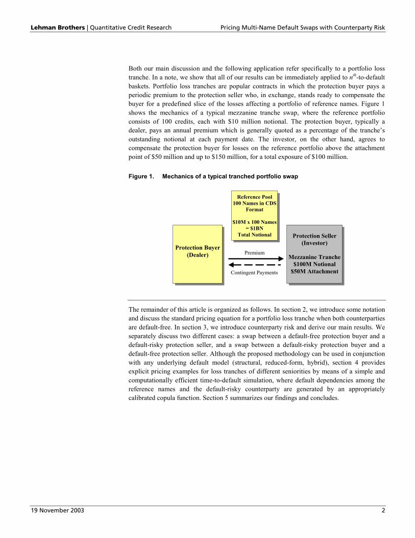
Both our main discussion and the following application refer specifically to a portfolio loss tranche. In a note, we show that all of our results can be immediately applied to nth-to-default baskets. Portfolio loss tranches are popular contracts in which the protection buyer pays a periodic premium to the protection seller who, in exchange, stands ready to compensate the buyer for a predefined slice of the losses affecting a portfolio of reference names. Figure 1 shows the mechanics of a typical mezzanine tranche swap, where the reference portfolio consists of 100 credits, each with $10 million notional. The protection buyer, typically a dealer, pays an annual premium which is generally quoted as a percentage of the tranche’s outstanding notional at each payment date. The investor, on the other hand, agrees to compensate the protection buyer for losses on the reference portfolio above the attachment point of $50 million and up to $150 million, for a total exposure of $100 million.

Figure 1. Mechanics of a typical tranched portfolio swap

Reference Pool 100 Names in CDS

Format

$10M x 100 Names = $1BN

Total Notional

Protection Seller (Investor)

Mezzanine Tranche

$100M Notional $50M Attachment

Protection Buyer(Dealer) Premium

Contingent Payments

The remainder of this article is organized as follows. In section 2, we introduce some notation and discuss the standard pricing equation for a portfolio loss tranche when both counterparties are default-free. In section 3, we introduce counterparty risk and derive our main results. We separately discuss two different cases: a swap between a default-free protection buyer and a default-risky protection seller, and a swap between a default-risky protection buyer and a default-free protection seller. Although the proposed methodology can be used in conjunction with any underlying default model (structural, reduced-form, hybrid), section 4 provides explicit pricing examples for loss tranches of different seniorities by means of a simple and computationally efficient time-to-default simulation, where default dependencies among the reference names and the default-risky counterparty are generated by an appropriately calibrated copula function. Section 5 summarizes our findings and concludes.


19 November 2003 3

2. FAIR DEFAULT SWAP SPREAD WITHOUT COUNTERPARTY RISK

Consider a default-free agent buying protection on a loss tranche from a default-free counter-party. If we denote with A the dollar exposure provided by the tranche, and with L(t) the cumulative dollar loss on the tranche at time t, we can compute the fair compensation for this exposure as the spread S which solves2:

( )

=

−⋅ ∫∑

=

MtM

iii tdLtBEtLAtBES

01

)()()()( . (1)

This expression simply equates the premium leg to the protection leg of the swap. The premium S is paid on the outstanding notional ( A - L(ti) ) at a set of predetermined dates ti, i=1,2,3...,M, while protection is paid at the time the loss is incurred. The expectation is taken with respect to the pricing measure, and all payments are discounted using the term structure of risk-free factors B(t).

Notice that equation (1) holds regardless of the assumptions made with respect to the sources of randomness (default times, recoveries and risk-free rates may all be stochastic) and the model used to generate their (risk-neutral) joint distribution.

To simplify the notation in the remainder of the paper, we introduce the following definitions:

( )∑=

−≡

k

jiii tLAtBkjN )()(),( , j ≤ k,

denotes the sum of discounted outstanding notional of the tranche between the jth and the kth payment dates, and

∫≡

v

u

tdLtBvuP )()(),( , u ≤ v,

denotes the sum of discounted payments received by the protection buyer between t=u and t=v. Notice that the distributions of the random variables N and P depend on the characteristics of the reference credits, such as their market spreads and default correlations, through the dependence on the portfolio loss distribution L. 3

Using these definitions, equation (1) can be conveniently rewritten as:

( )[ ] ( )[ ]MtPEMNES ,0,1 =⋅ . (2)

Note: nth-to-default swaps

Notice that equation (1) becomes the standard pricing equation for an nth-to-default basket swap if we substitute:

( ) ( ))(1 with )( ini tPtLA −− , and

)( with )( tdPLtdL nn ⋅ ,

2 To simplify notation, we do not explicitly consider accrual in any of our pricing equations. 3 The risk-neutral expectation of N(j,k) is often called the risky PV01 of a swap with payment dates tj, tj+1, …, tk-1, tk.


19 November 2003 4

where Pn(t) is a point process that jumps from 0 to 1 at the time of default of the nth reference name, and Ln is the loss-given-default of the nth defaulter (notice that, as long as default times are random, Ln is stochastic even if the loss-given-default of each reference name is assumed to be deterministic).

Using these definitions, everything that follows in this article can be immediately applied to nth-to-default basket swaps.

3. FAIR DEFAULT SWAP SPREAD WITH COUNTERPARTY RISK

In this section, we generalize the pricing of a tranched portfolio swap when one of the counterparties is also subject to default risk. For ease of exposition, we develop our arguments assuming that the default time of the risky counterparty is positively correlated with the default times of the names in the reference set. In reality, this is very often the case, since default events clearly have a systematic component. However, everything that follows can be adapted to a general dependence structure of default times.

3.1. Default-free protection buyer, default-risky protection seller To price a swap between a default-free protection buyer and a default-risky protection seller, we need to specify an assumption regarding the cashflows at the time of default of the risky counterparty. In what follows, we allow for an asymmetric recovery assumption {Q,R ; 0≤Q≤R≤1}, which indicates that the risk-free protection buyer will recover a fraction Q of the mark-to-market of the trade if this is in her favor, but will pay a possibly higher fraction R of the mark-to-market if this is against her. Notice that we allow for Q and R to be stochastic; therefore, when we write “Q≤R” or “Q=R”, we mean that the (in)equality holds for every element of the state space.4 We will denote with SQ,R the fair spread paid to a default-risky investor with a {Q,R ; 0≤Q≤R≤1} settlement in case of default.

We start with some necessary definitions. First, we introduce the additional notation:

=*τ default time of the default-risky protection seller, and

{ }Mt*,min ττ = ,

( ){ }τt:M,...,jz j ≤ ∈= ,21,0max .

In words, τ denotes the default time of the counterparty or the maturity of the deal, whichever comes first, and tz is the last payment date before τ.

Next, we define CPL as the (discounted) loss on the swap for the protection buyer as a result of the counterparty’s default:

( ) ( ) ( )MzNStPSCPL RQMRQ ,1, ,, +−= τ .

Finally, we define the (discounted) mark-to-market of the swap for the protection buyer at the time of the counterparty default, MTM, as

( ) ( )[ ] ( ) ( )[ ])(|,1,)(| ,,, τττ ℑ+−=ℑ= MzNStPESCPLESMTM RQMRQRQ , (3)

4 For example, we can model a stochastic mark-to-market recovery with Q≤R if we assume that Q and R are beta-

distributed on two non-overlapping supports.


19 November 2003 5

where, once again, the expectation is taken with respect to the pricing measure, and ( )τℑ denotes the information available at τ. Equation (3) states that the value of the swap at τ will be given by the difference between the value of the protection leg and the value of the premium leg at τ, and that the valuation will be done conditionally on the information

)(τℑ available at that time.

With this notation in place, we are now ready to write the pricing equation for a default swap between a default-free protection buyer and a default-risky protection seller:

( )[ ] ( )[ ] ( ) ( )( )[ ]RQRQRQ SMTMRSMTMQEPEzNES ,,, ,min,0,1 ⋅⋅+=⋅ τ (4)

The expression in (4) equates the present value of the premium paid up to τ to the present value of the protection received up to τ. In addition, the second term on the right-hand side indicates the present value of the (possibly negative) amount recovered by the protection buyer in case of default of the counterparty.

Our goal in this article is to price counterparty risk without explicitly calculating the mark-to-market of the swap in each state where the counterparty defaults. This would require, for each of these states, a derivation of the joint distribution of all stochastic variables conditional on the information set ( )τℑ ; for instruments with a large number of underlyings, such as portfolio loss tranches, this would be computationally expensive (see Schonbucher (2002)).

It turns out that our task is very simple if we impose the symmetric restriction Q=R, and that the solution to this symmetric problem paves the way for handling the more general (and more realistic) asymmetric recovery. For these reasons, we analyze these two cases separately.

3.1.1. The symmetric case: 0 ≤ Q = R ≤ 1

When 0≤Q=R=T≤1, equation (4) simplifies to:

( )[ ] ( )[ ] ( )[ ]TTTT SCPLTEPEzNES ,, ,0,1 ⋅+=⋅ τ ,

where we have used the law of iterated expectations and the fact that T is known at τ to conclude that:

( )[ ] ( )[ ]TTTT SCPLTESMTMTE ,, ⋅=⋅ .

Substituting for CPL and collecting terms gives:

( ) ( )[ ] ( ) ( )[ ]MTT tPTPEMzNTzNES ,,0,1,1, ττ ⋅+=+⋅+⋅ (5)

Equation (5) shows that the fair spread of this symmetric swap is equivalent to the fair spread on a “step-down” swap whose payments on both legs jump to T times the contractual payments at the time of default of the risky counterparty.

Once we specify the risk-neutral joint distribution of the stochastic variables in the model given the information available today, it is straightforward to compute ST,T. More precisely, the expectations in (5) can be obtained by simulating the stochastic variables in the model, calculating discounted premium and protection payments before and after the counterparty default along each path, and averaging across paths.

Notice also that when Q=R=T=1, equation (5) simplifies to (2), and S1,1 is therefore equal to S, the fair swap spread to be paid to a default-free protection seller. The intuition behind this


19 November 2003 6

result should be clear: if any amount due in case of default is fully recovered by the creditor, counterparty risk cannot have any impact on fair pricing.

On the other extreme, when Q=R=T=0, the swap knocks out and there is no additional inflow (or outflow) if the risky counterparty defaults. The fair value of the knockout spread S0,0 is simply determined by:

( )[ ] ( )[ ]τ,0,10,0 PEzNES =⋅ .

3.1.2. The asymmetric case: 0 ≤ Q ≤ R ≤ 1

An agent entering into a swap with a default-risky protection seller is generally concerned about the asymmetry of the potential mark-to-market settlement: it is likely that only a small fraction of a favorable mark would be recovered if the counterparty defaults, while it is possible that a negative mark would have to be paid in full. Of course, collateral agreements can mitigate the problem, but funding the trade may “kill” the economic rationale for the risky investor. For the pricing to reflect this asymmetry, we need to be able to deal with equation (4) under the assumption that Q≤R.

Solving for SQ,R exactly when Q≤R requires the calculation of the mark-to-market of the swap at τ, and this turns out to be computationally expensive even with the simplest model. Our strategy, therefore, will be to find bounds for RQS , and use their midpoint as an estimate; the

examples in the next section will then show that the proposed bounds are in fact very tight, so that the resulting maximum estimation error turns out to be very small.

The next two propositions identify an upper bound URQS , and a lower bound L

RQS , , such that:

URQRQ

LRQ SSS ,,, ≤≤ .

Proposition 1: An upper bound URQS , is given by QQS , .

First, observe that any symmetric solution TTS , , Q≤T≤R, is an upper bound for RQS , .

Intuitively, the default-free protection buyer is better off if:

1. the fraction of an unfavorable mark-to-market that she would have to pay in case her counterparty defaults decreases from R to T; and

2. the fraction of a favorable mark-to-market that she would recover increases from Q to T.

Therefore, the fair spread to be paid to the risky protection seller has to increase.

Next, notice that with positive dependence between the default time of the protection seller and the default times of the reference names, the mark-to-market in the event of default of the risky counterparty is expected to be in favor of the risk-free protection buyer. Therefore,

QQS , is the lowest of all upper bounds TTS , , Q≤T≤R, and therefore the one of interest to us.

Proposition 2: A lower bound LRQS , can be computed as the solution to:

( )[ ] ( )[ ] ( ) ( )( )[ ]LRQ

LRQ

LRQ SCPLRSCPLQEPEzNES ,,, ,min,0,1 ⋅⋅+=⋅ τ . (6)


19 November 2003 7

Equation (6) is analogous to (4), with the only difference that we have substituted MTM with CPL. By the law of iterated expectations and Jensen’s inequality we have, for any S5:

( ) ( )( )[ ]( ) ( )( ) ( )[ ][ ]( ) ( )[ ] ( ) ( )[ ]( )[ ]( ) ( )( )[ ]SMTMRSMTMQE

SCPLERSCPLEQESCPLRSCPLQEE

SCPLRSCPLQE

⋅⋅

=ℑ⋅ℑ⋅

≤ℑ⋅⋅

=⋅⋅

, min |, |min

|, min, min

ττ

τ

where we have used the fact that Q and R are known at τ, and the observation that, for 10 21 ≤≤≤ KK and ℜ∈x , ( )xKxK 21 ,min is a concave function of x.

A comparison between equations (4) and (6) is now sufficient to conclude that:

RQL

RQ SS ,, ≤ .

The crucial advantage of the proposed methodology is that these bounds can be obtained very easily, without explicitly calculating the value of the swap in the states where the risky counterparty defaults. We have shown earlier that the proposed upper bound

QQU

RQ SS ,, = can be computed as the solution to equation (5). The lower bound, LRQS , , can

be obtained by simulating the stochastic variables in the model, computing discounted premium and protection payments before and after the counterparty default along each path, and numerically solving for the value of L

RQS , that solves equation (6), ie, after substituting

for CPL,

( )[ ] ( )[ ]

( ) ( )( ) ( ) ( )( )( )[ ]. ,1,,,1,min

,0,1

,,

,

MzNStPRMzNStPQE

PEzNESL

RQML

RQM

LRQ

+−⋅+−⋅+

+=

ττ

τ

3.1.3. Window risk

Up to now, we have assumed that if the risky investor defaults, she will do so at a time when she does not owe any money to the protection buyer beyond, possibly, the mark-to-market of the swap. We may want to take into account the fact that, in reality, there is generally a lag between the moment when a loss affecting the tranche is experienced and the moment when the protection seller fulfills the associated obligation. If the counterparty defaults during this period, the protection buyer will suffer a direct loss that must be added to the potential cost of replacing the counterparty for the fulfillment of the remaining contractual obligations.

If we denote with ∆ the length of this window, we can see that the fair spread SQ,R now solves:

( )[ ] ( )[ ]

( ) ( )( )[ ] ( ) ( ) ( ) ( )( )[ ]∆−−⋅−⋅−⋅⋅+

+=⋅

τττ

τ

LLQBESMTMRSMTMQEPEzNES

RQRQ

RQ

1,min,0,1

,,

, (7)

Of course, the longer the window, the lower the fair spread will be. Bounds for SQ,R can be computed as explained earlier.

Notice that modeling window risk in this fashion allows us to account for counterparty risk in cases where the default-risky protection seller does not fund the losses throughout the life of the deal, but only at maturity. In this case, we would simply need to set ∆ =τ in equation (7) and notice that, by definition of cumulative loss, L(0)=0. 5 An alternative way to look at Proposition 2 is to recognize that, by definition, MTM dominates CPL in the sense of

second-order stochastic dominance (see Rothschild and Stiglitz (1970)).


19 November 2003 8

3.2. Default-risky protection buyer, default-free protection seller Analogous arguments can be used to find bounds for the fair spread paid by a default-risky protection buyer to a default-free protection seller. Let us slightly modify our previous definitions so that now:

=*τ default time of the default-risky protection buyer, and

{ }Mt*,min ττ = ,

( ){ }τt:M,...,jz j ≤ ∈= ,21,0max .

Also, a realistic recovery assumption can be represented by {R,Q ; 0≤Q≤R≤1}, in which we now denote with Q the fraction of a favorable mark-to-market that the default-free protection seller would recover, and with R the possibly higher fraction of an unfavorable mark that she would have to pay in the event of default of her risky counterparty.

With this notation in place, the equation for the fair swap spread QRS , is now given by

( )[ ] ( )[ ] ( ) ( )( )[ ]QRQRQR SMTMRSMTMQEPEzNES ,,, ,max,0,1 ⋅⋅+=⋅ τ . (8)

The expression in (8) equates the present value of the premium paid up to τ to the present value of the protection received up to τ. In addition, the second term on the right-hand side indicates the present value of the amount recovered (or paid) by the protection buyer in the event she defaults.

Following the same reasoning employed in the previous section, we can immediately identify bounds L

QRS , and UQRS , such that:

UQRQR

LQR SSS ,,, ≤≤ .

Proposition 3: A lower bound LQRS , is given by RRS , .

Proposition 4: An upper bound UQRS , can be computed as the solution to:

( )[ ] ( )[ ] ( ) ( )( )[ ]UQR

UQR

UQR SCPLRSCPLQEPEzNES ,,, ,max,0,1 ⋅⋅+=⋅ τ .

We conclude this section with the observation that the results obtained so far do not depend on any assumption made with respect to either the sources of randomness or the particular model used to generate their (risk-neutral) joint distribution.

4. APPLICATION: PRICING A SYNTHETIC LOSS TRANCHE

In this section, we offer a practical application of our methodology by pricing a tranched portfolio default swap. Our goal is to answer a number of questions:

1. What is the impact of counterparty risk on the fair spread of a synthetic loss tranche?

2. How do fair spreads vary in response to a change in the market-implied default probability of the risky counterparty?

3. How do fair spreads vary as default correlations between the risky counterparty and the reference names in the swap change?


19 November 2003 9

4. How do fair spreads vary as we change assumptions regarding the mark-to-market recovery at the time of default of the risky counterparty?

5. How tight are the bounds for the fair spread of a contract with asymmetric mark-to-market settlement? In other words, what is the maximum error that we incur in order to avoid the computationally expensive valuation of the remaining portion of the swap in each state where the risky counterparty defaults?

6. Using the fair spread of a swap between two default-free counterparties as a benchmark, is there any symmetry between: (a) the increase in fair spreads paid by a risky protection buyer to a risk-free protection seller; and (b) the decrease in fair spreads paid by a risk-free protection buyer to a risky protection seller?

To apply our methodology, we now have to specify which variables are random, and choose a model to produce their risk-neutral joint distribution. One simple and popular way to proceed is to employ a Gaussian copula to link the market-implied distributions of the default times of all defaultable credits, and add the simplifying assumptions of deterministic recovery rates and a deterministic risk-free term structure. Li (2000) shows that this approach to modeling default times can be interpreted as an extension of a one-period Merton’s model where default times and asset returns share the same correlation matrix.6

Following our discussion in section 3, we first consider a tranched portfolio default swap between a risk-free protection buyer and a default-risky protection seller.

4.1. Default-free protection buyer, default-risky protection seller

As highlighted in the previous sections, we can compute bounds for the fair spread of such a swap by simulating default times given only the information available today. We choose the following parameters for our base-case example:

1. We consider a 5-year default swap referring to a pool of 100 names, each with the same notional amount.

2. Each reference credit has a deterministic recovery rate of 35%.

3. Each reference credit, as well as the default-risky protection seller, has a yearly market-implied (risk-neutral) hazard rate of 2%.

4. Asset correlations between any two credits (including the risky counterparty) are all equal to 25%.

5. Q and R are assumed to be deterministic and equal to 35% and 1, respectively. This means that the risk-free protection buyer is going to recover only 35% of a positive mark-to-market but is going to pay in full for a negative mark-to-market if the protection seller defaults.

6. Every default in the reference set is immediately covered by the protection seller. In other words, there is no window risk as defined in section 3.1.3.

7. The risk-free curve is assumed to be deterministic. Risk-neutral cashflows are moved in time using the discount factors implied by the LIBOR curve as of October 2, 2003.

6 Mashal, Naldi and Zeevi (2003) provide empirical evidence supporting a fat-tailed generalization of this model.

Boscher and Ward (2002) study the consequences of allowing for stochastic recovery rates in this framework.


19 November 2003 10

Beyond the proposed bounds for the fair spread of this swap, we calculate the spread that would be fair if both counterparties were default-free. We compute these spreads for three tranches of different seniority: an equity piece covering the first 5% of the portfolio losses, a mezzanine tranche exposing the investor to the 5−10% slice of the losses, and a senior tranche absorbing the remaining defaults. Figure 2 shows the fair spreads for these tranches obtained from a 50,000-path Monte Carlo simulation. The numbers in parenthesis indicate the standard errors as percentages of the estimates, and show that 50,000 paths, requiring only a handful of seconds on a standard PC, are enough to drive down the standard errors to very reasonable levels.

Figure 2. Fair spreads (% std err in parenthesis). 50K-path Monte Carlo simulation

Equity (0−5%)

Mezzanine (5−10%)

Senior (10−100%)

Risk-Free Fair Spread 22.84% (0.44%) 6.980% (0.73%) 0.285% (1.16%) Upper Bound for Risky Fair Spread 22.56% (0.44%) 6.627% (0.77%) 0.250% (1.27%) Lower Bound for Risky Fair Spread 22.50% (0.44%) 6.576% (0.77%) 0.246% (1.27%)

To understand the magnitude of the error introduced solely by the fact that we compute bounds rather than the exact fair spread, we run a 5-million-path simulation to drive the standard errors down to insignificant levels. We then compute the maximum error that we can make by estimating the fair spread using the midpoint of the computed bounds. Figure 3 reports the results and shows that the proposed bounds are indeed quite tight. Intuitively, the adverse effect of the asymmetric recovery is dampened by the positive dependence between the default time of the protection seller and the default times of the reference credits, which implies that the mark-to-market of the swap is going to be in favor of the protection buyer in most states where the risky counterparty defaults.

Figure 3. Maximum error using midpoint. 5M-path Monte Carlo simulation

Equity (0−5%)

Mezzanine (5−10%)

Senior (10−100%)

Upper Bound for Risky Fair Spread 22.5516% 6.6148% 0.2499% Lower Bound for Risky Fair Spread 22.4986% 6.5637% 0.2463% Midpoint 22.5251% 6.5892% 0.2481% Max Error 2.65 bps 2.55 bps 0.18 bps

We now turn our attention to sensitivity analysis, and study how the bounds for the fair spreads of the three tranches described above change as we vary some of the input parameters.

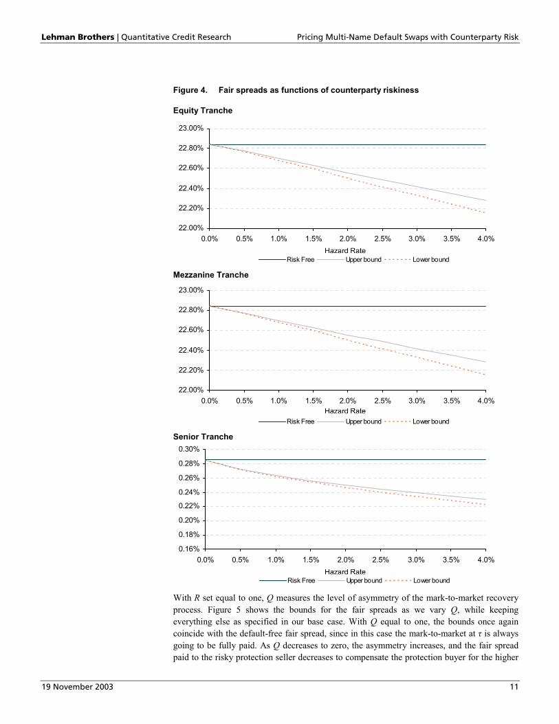
In Figure 4, we let the hazard rate of the protection seller vary between 0% and 4%, while keeping the same parameters for the reference portfolio as well as the same correlations among all credits. When the protection seller is risk-free, both bounds obviously coincide with the risk-free fair spread. As the hazard rate increases, both bounds decrease, and the interval they span becomes larger. Interestingly, the bounds become more convex in the hazard rate of the counterparty as we move up in seniority: since the senior investor will have to cover portfolio losses in very few scenarios, the marginal effect of an increase in her default probability is decreasing.


19 November 2003 11

Figure 4. Fair spreads as functions of counterparty riskiness

Equity Tranche

22.00%

22.20%

22.40%

22.60%

22.80%

23.00%

0.0% 0.5% 1.0% 1.5% 2.0% 2.5% 3.0% 3.5% 4.0%

Risk Free Upper bound Lower bound

Mezzanine Tranche

22.00%

22.20%

22.40%

22.60%

22.80%

23.00%

0.0% 0.5% 1.0% 1.5% 2.0% 2.5% 3.0% 3.5% 4.0%


Senior Tranche

0.16%

0.18%

0.20%

0.22%

0.24%

0.26%

0.28%

0.30%

0.0% 0.5% 1.0% 1.5% 2.0% 2.5% 3.0% 3.5% 4.0%


With R set equal to one, Q measures the level of asymmetry of the mark-to-market recovery process. Figure 5 shows the bounds for the fair spreads as we vary Q, while keeping everything else as specified in our base case. With Q equal to one, the bounds once again coincide with the default-free fair spread, since in this case the mark-to-market at τ is always going to be fully paid. As Q decreases to zero, the asymmetry increases, and the fair spread paid to the risky protection seller decreases to compensate the protection buyer for the higher

GGarnham

Hazard Rate

GGarnham

Hazard Rate

GGarnham

Hazard Rate


19 November 2003 12

expected loss in case of default. Both bounds increase almost linearly in Q for all tranches and, not surprisingly, the interval they span becomes smaller as the asymmetry of the mark-to-market settlement vanishes.

Figure 5. Fair spreads as functions of asymmetry of mark-to-market recovery

Equity Tranche

22.00%

22.20%

22.40%

22.60%

22.80%

23.00%

0% 10% 20% 30% 40% 50% 60% 70% 80% 90% 100%


Mezzanine Tranche

6.20%

6.40%

6.60%

6.80%

7.00%

7.20%

0% 10% 20% 30% 40% 50% 60% 70% 80% 90% 100%


Senior Tranche

0.16%

0.18%

0.20%

0.22%

0.24%

0.26%

0.28%

0.30%

0% 10% 20% 30% 40% 50% 60% 70% 80% 90% 100%


GGarnham

Q

GGarnham

Q

GGarnham

Q


19 November 2003 13

Finally, in Figure 6 we analyze the effect of varying the correlation between the risky protection seller and the credits in the reference portfolio, once again keeping the remaining parameters (including the correlations among the names in the reference set) at the levels fixed in the base case.

The first thing to notice is that our bounds are not tight at low levels of correlation. In particular, when the default time of the counterparty is independent of the default times of the reference credits, the expected mark-to-market of the swap at τ is close to zero (its exact value will generally depend on the shapes of the hazard rates and the risk-free curve). In this case, the only reason for which the spread paid to a risky protection seller should be lower than the one paid to a default-free investor is the asymmetry of the mark-to-market settlement. By definition, this effect cannot be captured by our upper bound, which is the fair spread for a (35%, 35%) symmetric swap, and is therefore very close to the risk-free fair spread.

The second thing to notice is the fact that fair spreads of different tranches behave very differently as we vary the correlation between the risky counterparty and the reference credits. At low levels of correlation, a correlation increase makes the expected mark-to-market at τ more favorable for the protection buyer, since a larger number of defaults are expected to affect the reference portfolio in the states where the counterparty defaults. Because the protection buyer now expects to lose a fraction (1-Q) of a larger mark-to-market, she has to pay a lower spread in order to break even. This holds true for tranches of all seniorities.

At high levels of correlation, however, an equity tranche is already exhausted at τ in a significant proportion of the states where the protection seller defaults. When this is the case, the mark-to-market of the equity swap at τ is obviously equal to zero. A further increase in correlation increases the frequency of such scenarios, and makes the expected mark-to-market at τ less favorable for the protection buyer. Because she now expects to lose a fraction (1-Q) of a smaller mark-to-market, the break-even spread has to increase.

The same reasoning holds for the mezzanine tranche, although the correlation level at which the fair spread reaches its minimum is higher. As far as the senior tranche goes, the fair spread generally decreases monotonically with the correlation between the risky counterparty and the reference credits.

One final observation we can draw from Figure 6 is that the sensitivity of the position of the risk-free protection buyer to an increase in correlation between the risky counterparty and the reference credits is higher for senior tranches than it is for junior tranches.


19 November 2003 14

Figure 6. Fair spreads as functions of correlation between c-p and reference credits

Equity Tranche

22.00%

22.20%

22.40%

22.60%

22.80%

23.00%

0% 5% 10% 15% 20% 25% 30% 35% 40% 45% 50%


Mezzanine Tranche

6.20%

6.40%

6.60%

6.80%

7.00%

7.20%

0% 5% 10% 15% 20% 25% 30% 35% 40% 45% 50%


Senior Tranche

0.16%

0.18%

0.20%

0.22%

0.24%

0.26%

0.28%

0.30%

0% 5% 10% 15% 20% 25% 30% 35% 40% 45% 50%


GGarnham

Correlation

GGarnham

Correlation

GGarnham

Correlation


19 November 2003 15

4.2. Default-risky protection buyer, default-free protection seller We now turn our attention to a swap between a default-risky protection buyer and a default-free protection seller. To compare the bounds for this swap with the ones obtained in the previous section, we keep working with the same base-case parameters on the understanding that:

1. it is now the protection buyer who has a yearly (risk-neutral) hazard rate equal to 2%; and

2. Q=35% is now the fraction of a favorable mark-to-market recovered by the default-free protection seller, while R=1 is the fraction of a favorable mark-to-market recovered by the default-risky protection buyer.

Notice that, from Proposition 3, the lower bound for the fair spread of this swap is given by 1,1S , which is also equal to the fair spread between two default-free counterparties.

Figure 7 shows the bounds for the fair spreads on the same three tranches defined earlier.

Figure 7. Fair spreads (% std err in parenthesis). 50K-path Monte Carlo simulation

Equity (0−5%)

Mezzanine (5−10%)

Senior (10−100%)

Upper Bound for Risky Fair Spread 22.89% (0.45%) 7.027% (0.74%) 0.289% (1.29%)

Lower Bound for Risky Fair Spread (=Risk-Free Fair Spread)

22.84% (0.44%) 6.980% (0.73%) 0.285% (1.16%)

The main observation we can draw from comparing Figure 2 with Figure 7 is that the default riskiness of the protection buyer produces an increase in fair spreads that is significantly smaller than the reduction in fair spreads resulting from the default riskiness of the protection seller. For example, the fair haircut for a 2% hazard rate protection seller on a 5-year mezzanine tranche is 35−40bp (Figure 2), while the fair surcharge for a 2% hazard rate protection buyer is certainly smaller than 5bp (Figure 7).

This difference is due to two main reasons. First, the distribution of the mark-to-market of a loss tranche at any given horizon is strongly asymmetric around zero, since it is bounded on one side by the outstanding notional of the tranche, and on the other by the present value of the remaining premium payments. Therefore, even with independence between the default time of the risky counterparty and the default times of the reference names, the asymmetry of the mark-to-market recovery has a larger impact on the expected loss due to counterparty default when the risky counterparty is the protection seller. Second, with positive default dependence between the risky counterparty and the reference names in the swap, a risky protection buyer tends to default when the mark-to-market is in her favor, while a risky protection seller tends to default when the mark-to-market is against her. For these reasons, allowing for the possibility of default of the protection seller has a much more significant impact on fair prices than allowing for the possibility of default of the protection buyer, other things being equal. Similar observations were made by O’Kane and Schloegl (2002) for single-name default swaps.


19 November 2003 16

5. SUMMARY

Pricing counterparty risk in multi-name default swaps is a challenging task. In principle, one needs to be able to evaluate the mark-to-market of the trade along each path in which the counterparty defaults, and precisely at the time where this default takes place. This, in turn, requires the calculation of the joint distribution of the default times of the surviving credits conditional on the information available at the time of default of the counterparty. In this article, we have suggested a simple methodology that tackles this computational complexity at its root, without imposing any restriction on the choice of the underlying joint default model.

In summary, we have derived two main results:

1. If the mark-to-market recovery is symmetric, then nested valuations are unnecessary and the contract can be exactly priced as a “step-down” swap, defined as a swap whose payments on both legs step down to a fraction of the contractual payments at the time of default of the risky counterparty.

2. If the mark-to-market recovery is asymmetric, as it is more realistic to expect, then bounds for the fair swap spread can be derived by means of a single simulation of joint defaults which uses only current information. These bounds turn out to be surprisingly tight when we have positive dependence between the default time of the risky counterparty and the default times of the reference names in the swap, which is also generally the case.

Applying these results to synthetic loss tranches of different seniorities, we have illustrated how their fair spreads vary as functions of a) the market-implied default probability of the risky counterparty, b) the asymmetry of the mark-to-market recovery at default, and c) the dependence between the default time of the risky counterparty and the default times of the credits referenced by the swap. Moreover, we have shown that allowing for the possibility of default of the protection seller has a much more significant impact on fair spreads than allowing for the possibility of default of the protection buyer, other things being equal.

We conclude with the observation that the methodology presented in this article can be easily extended to price swaps between two default-risky counterparties; the resulting bounds, however, will generally not be as tight as the ones derived above.

REFERENCES

• Boscher, H. and I. Ward, 2002, “Long or short in CDOs”, Risk, October, 125-129.

• Li, D. X., 2000, “On default correlation: a copula function approach”, Journal of Fixed Income, 9, 43-54.

• Mashal R., M. Naldi and A. Zeevi, 2003, “On the dependence of equity and asset returns”, Risk, October, 83-87.

• O’Kane, D. and L. Schloegl, 2002, “A counterparty risk framework for protection buyers”, Lehman Brothers, Quantitative Credit Research Quarterly, Q2.

• Rothschild, M. and J. Stiglitz, 1970, “Increasing risk: I. A definition”, Journal of Economic Theory, 2(3) 225-243.

• Schonbucher, P., 2002, “Copula-dependent default risk in intensity models”, Working Paper, ETH Zurich.

This material has been prepared and/or issued by Lehman Brothers Inc., member SIPC, and/or one of its affiliates (“Lehman Brothers”) and has been approved by Lehman BrothersInternational (Europe), regulated by the Financial Services Authority, in connection with its distribution in the European Economic Area. This material is distributed in Japan by LehmanBrothers Japan Inc., and in Hong Kong by Lehman Brothers Asia Limited. This material is distributed in Australia by Lehman Brothers Australia Pty Limited, and in Singapore by LehmanBrothers Inc., Singapore Branch. This document is for information purposes only and it should not be regarded as an offer to sell or as a solicitation of an offer to buy the securities orother instruments mentioned in it. No part of this document may be reproduced in any manner without the written permission of Lehman Brothers. We do not represent that thisinformation, including any third party information, is accurate or complete and it should not be relied upon as such. It is provided with the understanding that Lehman Brothers is notacting in a fiduciary capacity. Opinions expressed herein reflect the opinion of Lehman Brothers and are subject to change without notice. The products mentioned in this documentmay not be eligible for sale in some states or countries, and they may not be suitable for all types of investors. If an investor has any doubts about product suitability, he should consulthis Lehman Brothers’ representative. The value of and the income produced by products may fluctuate, so that an investor may get back less than he invested. Value and income maybe adversely affected by exchange rates, interest rates, or other factors. Past performance is not necessarily indicative of future results. If a product is income producing, part of thecapital invested may be used to pay that income. Lehman Brothers may make a market or deal as principal in the securities mentioned in this document or in options, futures, or otherderivatives based thereon. In addition, Lehman Brothers, its shareholders, directors, officers and/or employees, may from time to time have long or short positions in such securities or inoptions, futures, or other derivative instruments based thereon. One or more directors, officers, and/or employees of Lehman Brothers may be a director of the issuer of the securitiesmentioned in this document. Lehman Brothers may have managed or co-managed a public offering of securities for any issuer mentioned in this document within the last three years,or may, from time to time, perform investment banking or other services for, or solicit investment banking or other business from any company mentioned in this document.

2003 Lehman Brothers. All rights reserved.Additional information is available on request. Please contact a Lehman Brothers’ entity in your home jurisdiction.

Lehman Brothers Fixed Income Research analysts produce proprietary research in conjunction with firm trading desks that trade as principal in the instrumentsmentioned herein, and hence their research is not independent of the proprietary interests of the firm. The firm’s interests may conflict with the interests of aninvestor in those instruments.Lehman Brothers Fixed Income Research analysts receive compensation based in part on the firm’s trading and capital markets revenues. Lehman Brothers andany affiliate may have a position in the instruments or the company discussed in this report.The views expressed in this report accurately reflect the personal views of Marco Naldi and Roy Mashal, the primary analyst(s) responsible for this report, aboutthe subject securities or issuers referred to herein, and no part of such analyst(s)’ compensation was, is or will be directly or indirectly related to the specificrecommendations or views expressed herein.The research analysts responsible for preparing this report receive compensation based upon various factors, including, among other things, the quality of theirwork, firm revenues, including trading and capital markets revenues, competitive factors and client feedback.

To the extent that any of the views expressed in this research report are based on the firm’s quantitative research model, Lehman Brothers hereby certify (1) thatthe views expressed in this research report accurately reflect the firm’s quantitative research model and (2) that no part of the firm’s compensation was, is or will bedirectly or indirectly related to the specific recommendations or views expressed in this report.

Any reports referenced herein published after 14 April 2003 have been certified in accordance with Regulation AC. To obtain copies of these reports and their certifications,please contact Larry Pindyck ([email protected]; 212-526-6268) or Valerie Monchi ([email protected]; 44-207-011-8035).

Documents

Pricing Multi-Name Default Swaps with Counterparty … Brothers | Quantitative Credit Research Pricing Multi-Name Default Swaps with Counterparty Risk 19 November 2003 2 Both our main