Primary-Market Auctions for Event Tickets: Eliminating the Rents

of “Bob the Broker”?∗

Aditya Bhave† and Eric Budish‡

July 18, 2018

Abstract

Economists have long been puzzled by event-ticket underpricing: underpricing redu-ces revenue for the performer, and encourages socially wasteful rent-seeking by ticketbrokers. What about using an auction? This paper studies the introduction of auctionsinto this market by Ticketmaster. By combining primary-market auction data fromTicketmaster with secondary-market resale value data from eBay, we show that Tic-ketmaster’s auctions “worked”: they substantially improved price discovery, roughlydoubled performer revenues, and, on average, nearly eliminated the arbitrage profitsassociated with underpriced tickets. We conclude by discussing why, nevertheless, theauctions have failed to take off.

Keywords: market design, auctions, primary markets, resale markets, rent-seeking, posi-

tion auctions

∗We are grateful to Kip Levin and especially Debbie Hsu of Ticketmaster, for providing the Ticketmaster auctiondata and teaching us a great deal about event ticket markets. We are grateful to Adam Juda and Aaron Roth forthe Perl scripts we used to obtain eBay data. We thank Glenn Ellison and Steve Tadelis for valuable conferencediscussions. We thank Susan Athey, Sandeep Baliga, Hoyt Bleakley, Peter Coles, Ben Edelman, Jeff Ely, MattGentzkow, Philip Haile, Ali Hortacsu, Paul Klemperer, Alan Krueger, Julie Mortimer, Roger Myerson, Chris Nosko,Matt Notowidigdo, Michael Ostrovsky, Ariel Pakes, David Parkes, Canice Prendergast, Phil Reny, Al Roth, MichaelSchwarz, Jesse Shapiro, Alan Sorensen, Lars Stole, Chad Syverson, and Hal Varian for helpful conversations aboutthis research, as well as seminar participants at eBay Research, the University of Chicago, Duke, the 2012 NYU SternIO Day, Stanford, the 2012 NBER Market Design Working Group Meeting, the 2012 Michigan Auction and MatchingWorkshop, ACM EC 2013, the 2015 Econometric Society winter meetings, and the 2018 Music Industry ResearchAssociation annual conference. We thank Meru Bhanot, Mika Chance, Natalia Drozdoff, Sam Hwang, Yi Sun,and Cameron Taylor for excellent research assistance. Ticketmaster’s primary-market auction data were providedunder a confidentiality agreement, without restrictions on the right to publish other than that artists’ names be keptconfidential in the empirical analysis. Financial support from the National Science Foundation (ICES-1216083) andthe University of Chicago Booth School of Business is gratefully acknowledged.†Bank of America Merrill Lynch, aditya.bhave.17@gmail.com‡Corresponding author. University of Chicago Booth School of Business, eric.budish@chicagobooth.edu.

“It is nevertheless true that gangs of hardened ticket speculators exist and carry on

their atrocious trade with perfect shamelessness.” —New York Times Editorial (1876).

“Several decades ago I asked my class at Columbia to write a report on why successful

Broadway theaters do not raise prices much; instead, they ration scarce seats, espe-

cially through delays in seeing a play. I did not get any satisfactory answers, and

along with many others, I have continued to be puzzled by such pricing behavior.”

—Gary Becker (1991).

“We’re in an industry that prices its product worse than anybody else.” —Terry Barnes,

former chairman of Ticketmaster, in the Wall Street Journal (2006).

1 Introduction

In early 1868, Charles Dickens read from A Christmas Carol at Steinway Hall in New York City.

Tickets sold out in half a day at their face value of $2, and reportedly had a secondary-market value

of as high as $20; another report indicated that a young boy was paid $30 in gold for a good spot

in line (New York Times, November 1867 and December 1867). This phenomenon of event-ticket

underpricing – in which a performer, intentionally or not, sets a price for her event at a level at which

demand substantially exceeds supply – predates even Dickens (Segrave, 2007) and is widespread

in the present day (Leslie and Sorensen, 2014). For instance, when the Disney star Miley Cyrus

(aka Hannah Montana) first toured the US in 2007-2008, tickets with a face value of at most $64

sold out in approximately twelve minutes, and were then immediately posted on secondary-market

venues such as eBay and StubHub at prices that in some instances exceeded $2,000 (Levitt, 2008).

Tickets for the hit broadway show Hamilton sold out so quickly (sometimes in seconds), and were so

expensive in the secondary market (Mankiw, 2016), that its creator and star Lin-Manuel Miranda

began publicly advocating for changes to state ticket broker laws (Miranda, 2016).

Economists have long found this phenomenon puzzling (Becker, 1991, Landsburg, 1993, Rosen

and Rosenfield, 1997, Courty, 2003a, Baliga, 2011). First, underpricing reduces revenues for the

performer. Second, underpricing encourages socially wasteful rent seeking by ticket speculators.

While it is possible to tell stories for why performers may genuinely wish to sell tickets to their fans

1

at a below-market price – e.g., social-good consumption complementarities (Becker, 1991), altruism

(Che et al., 2013, though see also Bulow and Klemperer, 2012) or the sale of complementary goods

over the artist’s lifecycle (Mortimer et al., 2012) – it is hard to argue that artists genuinely wish for

ticket speculators to get tickets at below-market prices and earn arbitrage profits. In that sense,

the true puzzle is the combination of low prices and rent seeking by speculators due to an active

secondary market.

Modern information technology has only exacerbated the scale of this rent seeking. With both

the primary and secondary markets almost exclusively online, what used to be a localized, labor-

intensive activity in the pre-internet era now has few or no geographical boundaries and significant

scale economies. In the Dickens era, and as recently as the late 20th century, the basic rent-seeking

technology in the primary market was getting a good spot in a physical queue, and much of the

secondary market occurred outside the physical venue. A 1999 New York State Attorney General

report described “diggers” in the primary market – groups that “push and intimidate their way to

the front of the line” – and “scalpers” in the secondary market – individuals who stand “in front

of or near the venue for which tickets are being sold” (New York Attorney General, 1999). In the

present day, tickets can be amassed in the primary market online using software bots and sold in the

secondary market on websites such as eBay and StubHub (Zetter, 2010, Ticketmaster Blog, 2011a).

Recent industry estimates are that fully 20% of all tickets purchased in the primary market are

now resold in the secondary market, constituting on the order of $10-15bn of volume annually. In

extreme cases, speculators amass as many as 90% of the tickets available for a particular event.1 In

the colorful words of the Arkansas Attorney General, “All hell broke loose with Hannah Montana”

(Rosen, 2007).

Economic theory suggests there are two basic choices for how to curb this rent seeking. One

choice is to make tickets non-transferable, or otherwise ban resale. This would allow artists to set

whatever price they choose for their ticket, including an artificially low price (e.g., Hamilton awards

46 seats per night at $10 to fans who win a lottery, and prevents resale for these tickets (Paulson,

2016)). We will return to this idea in the conclusion, but note here that the legality of banning1The 20% figure is from a blog post by Ticketmaster’s CEO on 08/12/2011 (Ticketmaster Blog, 2011b), and the

$10-15bn order of magnitude figure is from Tan (2016). The 90% figure is a Ticketmaster estimate, based on softwareused to detect the software bots mentioned in the text. To give a sense of the growth of secondary market activity,Leslie and Sorensen (2014) report that the rate of resale was on the order of 5% in summer 2004 and report industryestimates that the overall secondary market size was about $3bn.

2

resale is fiercely debated, and an entire lobbying organization, the Fan Freedom Project – funded

in part by eBay and StubHub – is dedicated to preserving so-called “resale rights” (Lipka, 2011,

Fan Freedom Inc., Accessed in July 2017).

The second choice, of course, is to set a market-clearing price. This paper studies an effort

to do just that – Ticketmaster’s 2003 introduction of primary-market auctions for concert tickets.

Ticketmaster’s Chief Executive Officer remarked at the time:

“The tickets are worth what they’re worth. If somebody wants to charge $50 for a ticket,

but it’s actually worth $1000 on eBay, the ticket’s worth $1000. I think more and more

our clients – the promoters, the clients in the buildings and the bands themselves –

are saying to themselves ‘Maybe that money should be coming to me instead of Bob the

Broker.’” (Nelson, 2003. Emphasis added)

This paper shows that TM’s primary-market auctions “worked”: the auctions substantially im-

proved price discovery, roughly doubled artist revenues, and, on average, nearly eliminated the

arbitrage profits between the primary market and the secondary market.

Our empirical research design is very simple. We have proprietary data from TM, which indicate

the price at which each ticket was sold in TM’s primary-market auction, for all 2007 concert tours

that used auctions (we will describe the auction rules in detail below, which are interesting in their

own right). The data cover 22 distinct concert tours and 576 distinct concerts. We also have data

from TM that indicate, for each ticket sold by auction, what the fixed price would have been if not

for the auction; this is possible since only a relatively small number of tickets per event were sold by

auction, so it was always the case in our data that some tickets in the same quality tier as those sold

by auction were sold by fixed price.2 Last, we have data from eBay on the secondary-market values

of tickets sold by TM’s auction. Specifically, we scraped all instances where a ticket substantially

identical to a ticket sold in TM’s auction – a ticket to the same event, on the same date, in the

same section and row of the venue – subsequently sold on eBay.3 Given these three types of data,

it is straightforward to calculate the TM auctions’ effect on price discovery, revenues and arbitrage

profits.2For example, for many events all “floor” seats have the same fixed price (i.e., are in the same quality tier), while

only a fraction of floor seats are sold by auction.3The reason that we match tickets at the level of section and row, rather than the precise seat within the row, is

that for privacy reasons eBay listings do not indicate the specific seat. This was standard practice in the secondary

3

Figure 1: Relationship between eBay secondary-market values and TM primary-market prices, bothauction prices and face values

(a) Auction prices0

1000

2000

3000

eB

ay s

econdary

−m

ark

et valu

e

0 1000 2000 3000TM primary−market auction price

eBay secondary−market value unit−slope line

(b) Face values

01000

2000

3000

eB

ay s

econdary

−m

ark

et valu

e

0 1000 2000 3000TM face value

eBay secondary−market value unit−slope line

Notes: Panel (a) indicates the average primary-market auction price and secondary-market resale value for eachconcert-section-row in our matched dataset. Panel (b) indicates the ticket face value and average secondary-marketresale value for each concert-section-row in our matched dataset. Prices are on a per-ticket basis. eBay secondary-market values are net of eBay fees. For more details on the data, see the text of Section 5.

Figure 1 conveys our main results. The left panel is a scatterplot of TM primary-market auction

prices and subsequent eBay secondary-market resale values; each dot is a concert-section-row tuple

(e.g., The Police, 7/29/2007, Section A3, Row 2). The data mostly cluster along the 45-degree

line, which shows that the primary-market auction price is, on average, an accurate reflection of

secondary-market resale value. The mean difference between the auction price and the subsequent

resale value is just $6.07, or around 2% of the average primary-market auction price of $274. This

difference is economically small and statistically indistinguishable from zero. In the right panel,

instead of using the primary-market auction price, we use the ticket’s face value. Now, most of the

data are above the 45-degree line, sometimes dramatically so. This is the underpricing phenomenon.

The mean difference between the face value and the secondary-market resale value is now $136,

representing a 94% return on the average primary-market face value of $145.4 Moreover, the face-

value prices contain much less information about secondary-market values than do the auction

prices. In a regression of secondary-market value on primary-market prices, the R2 is 0.66 using

auction prices versus 0.24 using face-value prices. In sum, the auctions discover significantly higher

market at the time of our data. See Section 5.3 for more details.4The large magnitude is consistent with Leslie and Sorensen (2014)’s finding that the most severe underpricing

occurs for high-quality tickets, which are the focus of TM’s auctions.

4

prices than the counterfactual face values, and these prices are essentially correct on average. The

auctions essentially eliminate the scope for rent seeking, at least on average.

We also explore the auction performance of the most experienced bidders in the TM auction –

the top 1% of bidders, who account for 16% of volume. We find that the experienced bidders – the

“Bob the Brokers” – do in fact statistically outperform the inexperienced bidders, in the sense that

they purchase tickets in the auction with greater subsequent resale profits. However, the magnitude

of their profits is still relatively modest, at $19 per ticket, which is an order of magnitude smaller

than the $136 mean rent associated with purchasing primary-market tickets at their counterfactual

face values. This $19 per ticket can perhaps be interpreted as a return for the time, effort, and risk

associated with ticket speculation (cf. Courty, 2003a,b).

So far we have left vague the specific details of TM’s auction design. It turns out that the auction

TM designed is a variant on the position auctions that Google and other search engine firms use

for keyword advertising (Edelman et al., 2007, Varian, 2007). This similarity makes sense, because

in each case the auction is for a set of vertically-differentiated goods: in the keyword advertising

case, the goods are advertising slots of varying proximity to the top of the search page (e.g., first

slot, second slot, etc). In TM’s case, the goods are tickets of varying proximity to the stage (e.g.,

first row, second row, etc.).

There are two main differences between TM’s auction and the most widely used position auction

format, the Generalized Second Price (GSP) auction. The first difference is that in TM’s auction

successful bidders pay their own bid, rather than the next highest bid; that is the auction is more

like Generalized First Price (GFP) than GSP. However, while GFP has been heavily criticized in

the context of keyword auctions (Edelman and Ostrovsky, 2007), here the distinction between GSP

and GFP seems smaller, both because the auction is one-shot rather than repeated, and because the

difference in quality between successive prizes is small (e.g., there are many pairs of tickets in the

first row, many in the second row, etc.).5 TM perceived that the benefit of using pay-your-own-bid

is that it is simpler to explain to its customers. The second difference is the nature of bids: in

TM’s auction, bids are a per-ticket dollar amount, whereas typically in GSP bids are a per-click

dollar amount. This difference also makes sense for simplicity reasons, because it would be difficult

to bid on a “per-unit-quality” basis, whereas in the keyword advertising setting it is natural to bid5We thank Michael Schwarz for making this point.

5

on a per-click basis.

We provide a theoretical analysis of TM’s auction design, to complement the empirical analysis.

We begin by showing, in the context of an independent private values model adapted from that of

Edelman et al. (2007), that the Ticketmaster auction has an efficient equilibrium. This immediately

implies, via Myerson’s Lemma, that the TM auction is revenue equivalent to GSP, and to other

efficient auction designs such as Vickrey-Clarke-Groves. It also immediately implies that the TM

auction maximizes revenue subject to the constraint that all tickets are sold. Such a constraint

could be interpreted in the context of Becker (1991)’s observation that concerts that do not sell

out may see a discontinuous drop-off in demand, due to their social nature. We then add free entry

by speculators to the model, and show that entry eliminates arbitrage profits for these bidders.

We interpret this set of results – efficiency, constrained revenue maximization, and no arbitrage

for resellers – as formalizing that TM’s auction design is sensible.6 That said, bidding optimally

in the TM auction is strategically complex. We find evidence that bidders in TM’s auctions make

occasional large bidding errors associated with the pay-as-bid nature of the auction, and that these

errors are concentrated amongst inexperienced market participants. This suggests that there may

be gains from modifying TM’s auction format to be less strategically complex, e.g., the Purple

Pricing auction design proposed by Sandeep Baliga and Jeff Ely (cf. Baliga and Ely, 2013a,b).

We briefly mention three ways in which our results contribute to the broader market design

literature beyond the specific context of event-ticket markets. First, our results provide empirical

support for the proposition that, in markets with resale, sensibly designed primary-market auctions

accurately discover secondary-market resale values. This finding may be a useful input to market

design debates in other contexts, for instance, the debate over whether to use auctions in the

market for initial public offerings (IPOs). While there are of course many differences between

concert tickets and shares of stock, there are some important similarities: (i) both are non-trivial

to price; (ii) both have histories of severe underpricing; (iii) both have histories of elaborate rent-

seeking behavior associated with this underpricing (for IPOs, see, e.g., Nocera, 2013); and (iv) both

have secondary markets that are widely viewed to be efficient, suggesting that accurate pricing in

the primary market is a realistic possibility.6By contrast, Gomes and Sweeney (2014) show that the sealed-bid variant of GSP may not have an efficient

Bayes-Nash equilibrium in the Edelman et al. (2007) model; our results show that TM’s variant of GFP does havean efficient Bayes-Nash equilibrium in this model.

6

Second, our paper is, to our knowledge, the first empirical illustration of the usefulness of

position auctions in a context other than online advertising, and also documents a novel variant

on position auctions. These findings should be of interest to the literature on position auctions,

which has been extremely active since Edelman et al. (2007) and Varian (2007)’s studies of position

auctions for keyword advertising.

Third, our results serve as a case study in the use of market design to reduce rent seeking.

Perhaps the oldest objection to market design is to invoke the Coase theorem: market design

details do not ultimately matter, because private trade will eventually lead to the socially optimal

allocation.7 Paul Milgrom (Milgrom, 2004, Section 1.4.1) has called this “One of the most frequent

and misguided criticisms of modern auction design.” Our study is a reminder of why this argument

is flawed – even in the absence of Myerson-Satterthwaite bargaining frictions – because bad market

design can induce socially wasteful rent-seeking behavior on the way to the ultimate allocation (see

also Budish et al., 2015).

The remainder of this paper is organized as follows. Section 2 provides institutional background.

Section 3 describes Ticketmaster’s auction design. Section 4 presents the theoretical model. Section

5 describes our data. Section 6 presents our main empirical results. Section 7 compares experienced

and inexperienced bidders and discusses potential modifications to TM’s auction design. Section 8

concludes by discussing why TM’s auctions, despite “working” in the data, have failed to take off.

2 Institutional Background

“Primary market” refers to the original sale of tickets to an event, by or on behalf of the event

organizer. Ticketmaster, established in 1976, is the world’s largest primary-market ticket distribu-

tion company. In its most recent fiscal year, Ticketmaster sold more than 186 million event tickets

valued at on the order of $28 billion, on behalf of clients including venues, promoters, sports leagues

and teams, and museums and cultural institutions.8 Tickets are typically sold at fixed prices that7This argument was made to one of the authors of the present study on his first day on the faculty at the University

of Chicago, albeit over a friendly dim sum lunch.8Ticketmaster merged with Live Nation, a promoter, venue operator and artist management firm, in January 2010.

The 186 million tickets and $28bn figures are from Live Nation’s 2016 Q4 earnings report (Live Nation EntertainmentInc., 2017), and include Ticketmaster’s secondary market sales (approximately $1bn, Live Nation Entertainment Inc.,2016) in addition to its much-larger primary-market business. Live Nation also sold an additional 298 million ticketsthrough its clients’ box offices.

7

vary coarsely with seat quality, e.g., there might be just 3 or 4 pricing tiers in a venue with tens of

thousands of seats. Tickets typically go on sale months in advance of an event.

“Secondary market” refers to the resale of tickets purchased in the primary market. Ticketmas-

ter has estimated that 20% of all tickets purchased from Ticketmaster in the primary market are

subsequently resold on the secondary market (Ticketmaster Blog, 2011b). Recent industry reports

estimate that secondary-market dollar volume is on the order of $10bn in 2016, and will grow to

$15bn by 2020 (Tan, 2016). At the time of our data, eBay was the largest forum for secondary-

market activity (Mulpuru, 2008); at present the largest forum is StubHub ($4bn annually, eBay,

2017), which has grown substantially since eBay’s acquisition of it in 2007. Ticketmaster itself

entered the secondary market in 2002 with its launch of TicketExchange, and then increased its

presence in 2008 with its purchase of TicketsNow (Ticketmaster Entertainment LLC, 2010). Its

2015 secondary market volume was $1.2bn (Live Nation Entertainment Inc., 2016). See Sweeting

(2012) for a fascinating study of the dynamics of the secondary market, some findings from which

manifest in our data as well; see further discussion in Appendix A.

An important recent study by Leslie and Sorensen (2014) examines the welfare effects of the

secondary market, and finds empirical evidence of substantial costs and benefits of resale. The

main benefit is that it enables Pareto-improving reallocation of tickets, e.g., resale by fans who

no longer can attend the event. The main cost is the rent-seeking activity that the possibility of

resale encourages in the primary market. In Leslie and Sorensen (2014)’s analysis, if price could be

set correctly in the primary market such that rent-seeking activity is eliminated, the main cost of

allowing resale would be eliminated as well. Our paper suggests that this is possible via auctions.

While secondary-market activity has been a part of the event-ticket market for a long time (see

the quotes in the introduction), its scale seems to have increased dramatically with the rise of the

internet.9 There are at least three reasons. First, the internet has lowered the costs of amassing

tickets in the primary market.10 Second, the internet has lowered the cost of reselling tickets in the

secondary market. Third, the internet has made it easier to skirt state rules on ticket reselling (cf.9See the New York Attorney General’s 1999 report “Why Can’t I Get Tickets?” (New York Attorney General,

1999), for an excellent primer on pre-internet ticket reseller tactics.10For instance, Ticketmaster writes on its corporate blog: “There continue to be nefarious online scalpers who use

sophisticated tools – often known as bots – to cut in line ahead of you and scoop up large quantities of tickets, onlyto turn around and sell them to fans at many times the face value of the tickets. The use of these bots is illegal, itviolates our terms of use, and it is on the rise. Worst of all, these bots prevent you from getting a fair shot at ticketsto the event you want to see live” (Ticketmaster Blog, 2011a).

8

Courty, 2000, 2003a, Connolly and Krueger, 2006).

Technology has also changed the publicness of the secondary market, e.g., any ordinary fan can

now look up the secondary-market value of their tickets on eBay. Roth (2007) speculates that this

may have caused a decline in the “repugnance” associated with charging high prices for tickets in

the primary market, a trend that has manifested both in the use of auctions and in the use of

higher fixed prices than in previous eras (cf. Connolly and Krueger, 2006).

3 Ticketmaster’s Primary-Market Auction

In 2003 Ticketmaster introduced auctions as a primary-market pricing method, alongside fixed

price. As discussed in the introduction, Ticketmaster emphasized eliminating the arbitrage profits

of “Bob the Broker”; the initial clients who adopted auctions also emphasized this idea that tickets

are “worth what they are worth” and hence auctions are fair.11 In this section we describe the rules

of the auction in detail.

Which Tickets are Auctioned? For any particular event, the determination of which tickets

to sell by auction (if any), and which to sell by fixed price, is made by TM’s client. In our data,

an average of about 97 tickets are auctioned per concert, with a maximum of 862 tickets. The

auctioned tickets are always of high quality, often in the first few rows of the venue, allowing the

auction to be positioned in TM’s marketing efforts as “premium seat auctions”. This decision to

focus on high-quality tickets is consistent with Leslie and Sorensen (2014)’s finding that high-quality

tickets are associated with the most underpricing and inefficient rent-seeking. TM and the client

organize the auction tickets into discrete quality groups, typically by rows. For instance, in the

auction depicted in Figure 2, the first quality group is “Section A3, A4 or A5, Row 2”, the second

“Section A3, A4 or A5, Row 3”, etc. TM and the client also rank the tickets by quality within each

group. For instance, within Row 2, tickets in Section A4 are ranked above those in Sections A3

and A5 because Section A4 is more centrally located. The groups are designed, however, so that

quality heterogeneity within a group is small.11Said Timothy J. Leiweke, President of the Staples Center in Los Angeles, which hosted the first event to use a

Ticketmaster auction: “Market inefficiencies ... highlight the need for the event promoter to establish prices for liveevent ticketing closer to what the consumer is ultimately willing to pay. One way to establish a fair price for the besttickets is through an online auction, open to the general public, allowing the market to determine the price” (EastSide Boxing, 2003).

9

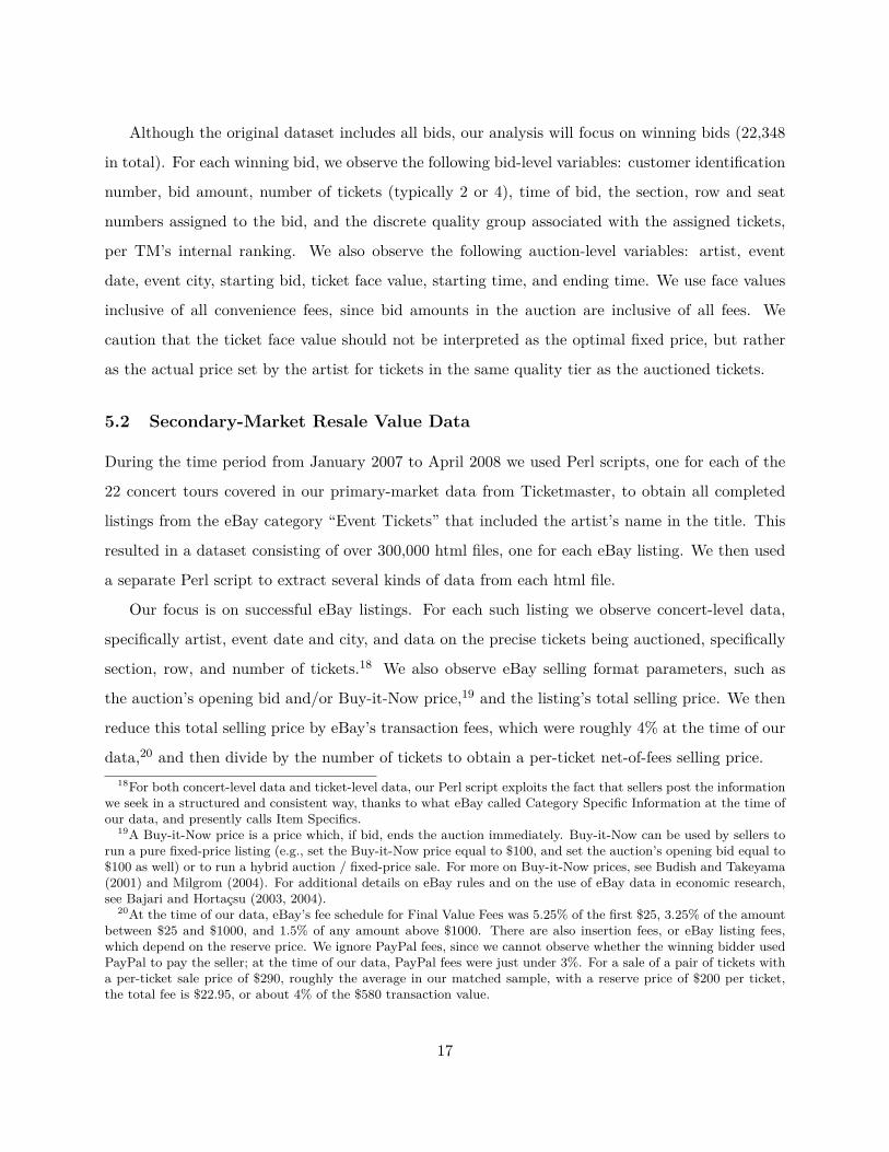
Figure 2: User interface for the Ticketmaster primary-market auction

Notes: This screenshot was taken from the Ticketmaster primary-market auction for tickets to see The Police inFenway Park, Boston, July 29, 2007.

Auction Rules The auction itself lasts for several days, starting and ending at pre-announced

fixed times. The auction dates typically are timed to coincide with the sale of other tickets by fixed

price, for marketing reasons; e.g., in the auction depicted in Figure 2, the auction opened on a

Sunday and ended on a Friday, while the bulk of fixed-price tickets went on sale on the intervening

Tuesday.

The auction has a non-zero per-ticket starting bid, which is set to be approximately equal to

the fixed price (i.e., face value) of other tickets in the same quality tier as the auctioned tickets.12

Bids consist of a per-ticket dollar amount and a desired number of tickets, e.g. 2 or 4. Bidders

can increase their bid amount at any time throughout the auction, but bidders are not allowed to

lower or retract their bids. At the conclusion of the auction, bids are sorted in descending order,

with the highest bid winning the best tickets within the highest quality group, the next highest12Auction bids are inclusive of convenience fees, whereas fixed-price tickets have separately stated face values and

convenience fees. The starting bid in the auction is typically set equal to the face value plus convenience fees of ticketsin the same quality tier as the auctioned tickets, rounded to a multiple of $10 or $25. For instance, in the auctiondepicted in Figure 2, the face value for tickets in the same quality tier as the auction was $225 and convenience feeswere $21.60, for an all-in fixed price of $246.60, and the auction starting bid was set to be $250. Throughout thepaper, when we refer to a ticket’s face value or fixed price, we mean the price inclusive of convenience fees.

10

bid winning the next best tickets in the highest quality group, etc. Ties are broken by order of bid

receipt. Successful bidders pay their bid amount; losing bidders pay zero.

Over the course of the auction, bidders can view the current market-clearing prices by group.

For instance, in the auction depicted in Figure 2, there are enough bids of $540 and higher to fill

the first quality group, enough bids of $420 and higher to fill the first two quality groups, etc.

Additionally, bidders receive email notifications whenever their current bid’s tentative assignment

drops down a quality group. For instance, if the cutoff for the first quality group had just increased

from $530 to $540, any bidders of $530 would just have received a notification.

Starting in April 2007, bidders could also specify a quality threshold indicating the lowest

quality group that their bids were valid for (e.g., valid only for the first 3 quality groups). As

before, at the end of the auction, bids are sorted in descending order with the highest bid winning

the highest-quality tickets, etc. The only modification is that if a bid is reached where the quality

that would be awarded is below the bidder’s threshold, then that bid is skipped.

4 Model

In this section, we provide a theoretical analysis of the Ticketmaster primary-market auction design,

focusing on the original 2003 auction rules. Our analysis both clarifies the relationship between

the TM auction design and the position auctions used widely in internet advertising markets, and

formalizes that the TM auction design is “sensible” in that it satisfies attractive efficiency, revenue

and no arbitrage properties.

Our model closely mirrors that of Edelman et al. (2007). There are K (pairs of) tickets and

n > K ex-ante symmetric, risk-neutral bidders.13 Initially, we think of a bidder as either a fan

who intends to use the tickets herself, or as a speculator acting as a proxy agent on behalf of a

specific fan. Below we will endogenize entry by speculators, in a stylized manner, to derive a simple

no-arbitrage result. The tickets are vertically differentiated, with bidder i’s private valuation for

the kth-best ticket equal to αkvi: vi is bidder i’s type, and αk describes the quality of ticket k,13For expositional purposes, we will refer to a pair of tickets simply as one object, or one ticket.

11

with α1 > α2 > · · · > αK .14 We assume that the quality levels are common knowledge, and we

normalize αK = 1.

Each bidder’s type vi is drawn independently and identically from a distribution with cdf F (·)

and support [0, v̄]. We assume that F (·) is continuously differentiable, with f (·) the corresponding

pdf. The distribution of preferences is common knowledge.

We consider two ways to model the Ticketmaster auction design, sealed-bid and ascending

auction, analogously to how Edelman et al. (2007) consider both a sealed-bid and ascending

auction variant of GSP. The sealed-bid model captures the fact that the TM auction uses a “hard-

close” ending rule (cf. Roth and Ockenfels, 2002), and highlights that bidders are uncertain, at the

moment they bid, of what quality ticket they will win, and indeed whether they will win any ticket

at all. However, the TM auction is not static, and in particular bidders do have some information

at the time they bid about the demand of other bidders (see Figure 2 in the main text). Hence we

also consider an ascending auction model, for completeness. Our main theory results – on efficiency,

constrained revenue maximization, and no arbitrage – obtain under both models.

In the sealed-bid TM auction model, each bidder submits a single bid. The bids are ranked in

descending order, and then the kth-highest bidder wins the kth ticket, for each k = 1, . . . ,K. There

is no reserve price. Winning bidders pay their bid amount, while losers pay nothing. To explain

the difference between this model and Edelman et al. (2007)’s model of GSP, let b(k) denote the

kth-highest bid, for some k ≤ K. In GSP, the kth-highest bidder’s total payment is b(k+1)αk: the

next-highest bid, times the click-through rate. In our model, this bidder’s total payment is simply

b(k): her own bid, without any adjustment for the realized quality.

Our ascending TM auction model is related to the Generalized English Auction (GEA) of

Edelman et al. (2007), analogously to how our sealed-bid model is related to their treatment of

GSP. An auction clock, initialized at p = 0, ascends continuously at the rate of $1 per unit time.

Bidders can “drop” out of the auction at any time; once a bidder drops out of the auction, the

auction is over for her (cf. Milgrom and Weber, 1982). The auction ends when all bidders but one

have dropped. The last remaining bidder gets the best ticket, and pays the amount at which the

next-to-last bidder dropped. The kth-to-last remaining bidder, for k = 2, . . . ,K, gets the kth ticket,

and pays the amount at which she herself dropped. The n−K bidders who do not get a ticket pay14In Edelman et al. (2007), αk is the click-through rate of the kth slot, and vi is the ith advertiser’s private value

per click.

12

zero.

4.1 Efficiency and Revenue Results

4.1.1 Efficiency

Equilibrium of the Sealed-bid TM Auction Let Pk(v) denote the probability that a bidder

whose type is v has the kth-highest type out of the n bidders. We show the following.

Proposition 1. (Efficiency of Sealed-Bid Auction) There exists a symmetric monotonic Bayes-

Nash equilibrium of the sealed-bid TM auction in which all bidders bid according to

b (v) = 1∑Kk=1 Pk (v)

(K∑k=1

Pk (v) (vαk)−K∑k=1

∫ v

0αkPk (x) dx

). (1)

The resulting allocation is efficient.

Function (1) can be interpreted as follows. The first term,∑K

k=1 Pk(v)(vαk)∑K

k=1 Pk(v), is bidder v’s expec-

tation of the value of the ticket she will receive, conditional on being one of the k winners. Note

that this term will be strictly between the value she places on the best ticket, α1v, and the value

she places on the worst ticket, αKv. The second term,∑K

k=1

∫ v0 αkPk(x)dx∑K

k=1 Pk(v), is the amount by which

she shades her bid due to the pay-as-bid nature of the auction. If K = 1 this is just the standard

single-unit auction information rent. When K > 1, the numerator places relatively more weight,

in determining how much to shade, on tickets that are of high quality (the αk term) and on tickets

where bidder v’s value is high enough that it is likely that someone with a lower value than she

wins those tickets (the∫ v

0 Pk (x) dx term). Intuitively, if a ticket is of very low quality (low αk), or

if bidder v is not really in the running for the ticket (the∫ v

0 Pk (x) dx term), then she should not

earn an information rent from that ticket.

Equilibrium of the Ascending TM Auction Consider a bidder of type v. Let v be the lowest

possible type who has not dropped out when all other bidders are following symmetric equilibrium

strategies. At a given point in time, aside from the bidder in question, suppose that there are

k other active bidders in the auction. Then let T (v; v, k) denote the amount of time bidder v

would be willing to wait before dropping out, conditional on the event that none of the other active

13

bidders drop out during this time. Additionally, define the hazard rate in the standard manner,

h (v) = f(v)1−F (v) .

Proposition 2. (Efficiency of Ascending Auction) The unique symmetric perfect Bayesian equili-

brium of the ascending auction is defined by,

T (v; v, k) =

v − v, if k ≥ K,

(αk − αk+1)∫ vv xkh (x) dx, if k < K.

(2)

The resulting allocation is efficient.

The equilibrium of the ascending auction can be understood as follows. Given a bidder with

value v, as long as there are at least K other active bidders in the auction she behaves as if she is

competing in a standard K + 1st-price auction for K units of ticket K. That is, she simply bids up

to her value for the Kth ticket of vαK ≡ v , i.e., her waiting time is v− v. Once ticket K has been

allocated the game changes in an important way: now, bidder v behaves as if she is competing in

an all-pay auction against K − 1 other bidders for the quality increment αK − αK−1. That is, she

is competing for the right not to wind up with ticket K. The all-pay nature of the auction follows

from the fact that waiting is now costly: since she is a winner in the auction, she must pay her bid.

If she survives this auction, she competes against the K − 2 other remaining bidders in an all-pay

auction for the quality increment αK−1 − αK−2, and so forth. The intuition for the equilibrium

waiting time is as in Bulow and Klemperer (1999): bidders equate their marginal cost of waiting,∂T (v;v,k)

∂v , with their marginal benefit from doing so, (αk − αk+1) vkh (v). In the Appendix, we prove

by induction that the above collection of individual auction equilibria constitutes an equilibrium of

the full ascending TM auction game.

4.1.2 Revenue

By Myerson’s Lemma (cf. Milgrom, 2004), since the equilibria described in Section 4.1.1 lead to

an efficient allocation, and the lowest type gets zero surplus, we immediately have the following

corollary:

Corollary 1. (Revenue Performance) The sealed-bid and ascending Ticketmaster auctions are

revenue equivalent to any other efficient auction design in which the lowest type gets zero surplus,

14

such as GSP or Vickrey-Clarke-Groves.

Myerson’s Lemma also implies the following corollary regarding the revenue performance of the

TM auction:

Corollary 2. If v− 1−F (v)f(v) is strictly increasing, the sealed-bid and ascending Ticketmaster auctions

each maximize revenue subject to the constraint that all tickets are always sold.

The constraint that all tickets are always sold can be interpreted in the context of Becker

(1991)’s observation that concerts that do not sell out may see a discontinuous drop-off in demand,

due to their social nature. An optimally set reserve price would increase revenue in our model, but

would risk leaving some tickets unsold. Together, Propositions 1 and 2 and Corollaries 1 and 2

indicate that TM’s auction has attractive efficiency and revenue performance.

4.2 No Arbitrage

So far our analysis has treated the set of bidders as exogenous; these bidders were conceptualized

either as fans or as professional resellers acting as proxies on behalf of specific fans.

In this section we allow for endogenous entry by professional resellers, in the following stylized

manner. There is a continuum of potential bidders in the population, of which a fraction β are

professional resellers, and the remaining are fans. Fans’ types are drawn independently and iden-

tically from the continuously differentiable distribution Ffan(·) with support [0, v̄]. Fix ε > 0 and

w ∈ (ε, v̄). Each reseller’s type is drawn independently and identically from the continuously diffe-

rentiable distribution Fpro(·) with support [w − ε, w]. The interpretation is that w is the expected

price (per unit quality) of a ticket on the secondary market. Resellers also face a small idiosyncra-

tic cost, in the interval [0, ε], associated with participating in the aftermarket. The purpose of the

idiosyncratic cost is to ensure that Fpro(·) can be assumed to be atomless.

In each auction, n bidders are randomly drawn from the above population of potential bidders.

Notice that this process is equivalent to taking n i.i.d. draws from the distribution F (·), where

F (x) = βFpro (x) + (1− β)Ffan (x) . (3)

F (·) has support on [0, v̄], and we assume that F (·) is continuously differentiable ∀β ∈ [0, 1].15

15Since the support of Fpro is a subset of that of Ffan, this is equivalent to assuming that (i) F ′pro (w − ε) = 0 or

15

This method of constructing a population comprising professional resellers and fans allows us to

use the symmetric bidding equilibria that we derived in Propositions 1 and 2.

Let npro ≡ βn and nfan ≡ (1− β)n denote, respectively, the expected number of professional

resellers and fans in the auction. We then model entry by speculators by allowing npro to increase

while nfan remains constant. This approach to endogenizing entry allows for the following simple

no arbitrage statement.

Proposition 3. (No Arbitrage) Let s (v;npro, nfan) denote the expected surplus, conditional on

winning some ticket, of a professional reseller with value v. Under either the sealed-bid or ascending

TM auction, for any v ∈ [w − ε, w] and any finite nfan, limnpro→∞ s (v;npro, nfan) = 0.

Proposition 3 formalizes in a simple manner that free entry by speculators causes them to earn

negligible resale profits, even when we condition on the event that they win a ticket in the auction.

Though a simple result, it highlights an important difference between auctions and fixed-price

selling mechanisms.

5 Data

Our data come from two sources: primary-market auction data provided by Ticketmaster, and

secondary-market resale value data scraped from eBay. Sections 5.1 and 5.2 describe each dataset

in turn. Section 5.3 describes how the datasets are matched.

5.1 Primary-Market Auction Data

Our primary-market auction data cover all Ticketmaster auctions for concert tours that started

in 2007. There are 22 concert tours, 576 concerts, and 759 auctions.16,17 The concerts took place

between March 2007 and April 2008, and the corresponding auctions were conducted between

January 2007 and December 2007.

w = ε, and (ii) F ′pro (w) = 0 or w = v̄.16For the majority of concerts there is just a single auction, but in some cases there are 2 or more auctions for the

same event. For instance, it is somewhat common for there to be a separate auction for tickets in the first row. Thiscan be understood as an auction design response to the large perceived difference in quality between the first andsecond rows; e.g., under TM’s original bidding language (pre April 2007), such a difference would have caused therefrequently to be bidders with negative realized surplus.

17We drop all concerts in Canada. These concerts comprise less than 2% of our primary-market dataset.

16

Although the original dataset includes all bids, our analysis will focus on winning bids (22,348

in total). For each winning bid, we observe the following bid-level variables: customer identification

number, bid amount, number of tickets (typically 2 or 4), time of bid, the section, row and seat

numbers assigned to the bid, and the discrete quality group associated with the assigned tickets,

per TM’s internal ranking. We also observe the following auction-level variables: artist, event

date, event city, starting bid, ticket face value, starting time, and ending time. We use face values

inclusive of all convenience fees, since bid amounts in the auction are inclusive of all fees. We

caution that the ticket face value should not be interpreted as the optimal fixed price, but rather

as the actual price set by the artist for tickets in the same quality tier as the auctioned tickets.

5.2 Secondary-Market Resale Value Data

During the time period from January 2007 to April 2008 we used Perl scripts, one for each of the

22 concert tours covered in our primary-market data from Ticketmaster, to obtain all completed

listings from the eBay category “Event Tickets” that included the artist’s name in the title. This

resulted in a dataset consisting of over 300,000 html files, one for each eBay listing. We then used

a separate Perl script to extract several kinds of data from each html file.

Our focus is on successful eBay listings. For each such listing we observe concert-level data,

specifically artist, event date and city, and data on the precise tickets being auctioned, specifically

section, row, and number of tickets.18 We also observe eBay selling format parameters, such as

the auction’s opening bid and/or Buy-it-Now price,19 and the listing’s total selling price. We then

reduce this total selling price by eBay’s transaction fees, which were roughly 4% at the time of our

data,20 and then divide by the number of tickets to obtain a per-ticket net-of-fees selling price.18For both concert-level data and ticket-level data, our Perl script exploits the fact that sellers post the information

we seek in a structured and consistent way, thanks to what eBay called Category Specific Information at the time ofour data, and presently calls Item Specifics.

19A Buy-it-Now price is a price which, if bid, ends the auction immediately. Buy-it-Now can be used by sellers torun a pure fixed-price listing (e.g., set the Buy-it-Now price equal to $100, and set the auction’s opening bid equal to$100 as well) or to run a hybrid auction / fixed-price sale. For more on Buy-it-Now prices, see Budish and Takeyama(2001) and Milgrom (2004). For additional details on eBay rules and on the use of eBay data in economic research,see Bajari and Hortaçsu (2003, 2004).

20At the time of our data, eBay’s fee schedule for Final Value Fees was 5.25% of the first $25, 3.25% of the amountbetween $25 and $1000, and 1.5% of any amount above $1000. There are also insertion fees, or eBay listing fees,which depend on the reserve price. We ignore PayPal fees, since we cannot observe whether the winning bidder usedPayPal to pay the seller; at the time of our data, PayPal fees were just under 3%. For a sale of a pair of tickets witha per-ticket sale price of $290, roughly the average in our matched sample, with a reserve price of $200 per ticket,the total fee is $22.95, or about 4% of the $580 transaction value.

17

Figure 3: eBay auction webpage for tickets that were sold in the Ticketmaster auction shown inFigure 2

An example of an eBay auction webpage is depicted as Figure 3. This eBay listing was for a

pair of tickets in Section A3, Row 3 to see the Police at Fenway Park on July 29, 2007; this is the

same concert whose TM auction webpage we depicted above in Figure 2. This eBay listing resulted

in a total sale price of $999.99, or $499.995 per ticket before fees.

Unlike the primary-market data, we do not observe seat numbers in the eBay data. For instance,

notice in Figure 3 that Section and Row are data fields that eBay allows the seller to fill in (and

that this particular seller did fill in), but that there is no such data field for seat number.21 Thus

when comparing the primary and secondary markets, we conduct our analysis at the section-row

level, as described in Section 5.3.

We drop all observations in which just a single ticket was sold, because prices for individual

tickets are not representative of per-ticket prices for sets of two or more tickets (most consumers

wish to attend concerts in groups rather than alone). We also drop observations in which the seller

elected to use eBay’s “Dutch auction” format for selling variable quantities of tickets, because eBay

sellers are inconsistent about whether they complete the “Number of Tickets” field on the eBay

webpage based on the number of tickets awarded per winning bid (typically 1, 2 or 4) or based on21Listing tickets at the section and row but not seat level is a common practice on all of the secondary market

websites of which we are aware. See further discussion of this issue in Section 5.3.

18

the total number of tickets the seller has available. As a result we are unable to reliably compute

the price paid per ticket. Together, single-ticket and Dutch auction observations comprise about

14% of our eBay listings.

5.3 Matching Primary- and Secondary-Market Data

In this section we describe our procedure for matching the Ticketmaster primary-market data to

the eBay secondary-market data. There are three specific issues that are important to highlight.

First, the eBay data indicate the section and row in which the auctioned tickets are located,

but not the precise seat numbers. This was standard practice in the secondary market for tickets

at the time of our data, both for seller privacy reasons and because quality heterogeneity within

a section-row is usually of negligible importance relative to the importance of the section and row

information.22,23 For this reason, we match the two datasets at the level of the concert-section-row

(“c-s-r”).

Second, eBay section and row data are input by eBay sellers, and are non-standardized. For

instance, eBay sellers typically use the string “1” in the Row field to describe tickets that are in

Row 1, but we also observe entries of “#1”, “**1**”, “1st”, “1 !!!!”, “First”, “one”, “1 WOW!”, and

dozens of others. We handle this issue as follows. First, we create a dictionary that translates all

observed eBay row input strings into standardized terms; e.g., all of the Row entries listed above

get translated into “1”. We then create a venue-specific section dictionary, which translates each

observed eBay section input string into a section name that appears on the seating chart of the

venue for the event in question. Last, we match the eBay data to the Ticketmaster data at the

level of concert-section-row, using the two dictionaries.

Third, when a particular c-s-r tuple has multiple TM primary-market auctions and/or multi-

ple eBay secondary-market transactions, an issue arises as to how exactly to match the two sets

of transactions. Our main specification for the analyses in Section 6 performs this match by ag-22In addition to typically being of negligible importance, seat data are also typically difficult to interpret. For

instance, for the auction depicted in Figure 2, the Fenway Park concert seat map indicates that Section A4 is slightlymore centrally located than Sections A3 and A5, and it is obvious that “Row 2” is higher quality than “Row 3”, butinformation on what seat number is most centrally located within Section A4 - Row 2 is not readily available. As itturns out there are 24 seats within this row, and seats 12 and 13 are the most centrally located.

23While seat data being of negligible importance is typical, there are a handful of venues where heterogeneity inseat quality within a row is of sufficient importance that Ticketmaster demarcated distinct quality groups within arow in the auction. As a robustness exercise, we omitted these venues from the analysis; the results moved very little.

19

Table 1: Summary statistics for matched primary- and secondary-market data

Full TM Data Set Matched Data Set % MatchedConcerts 576 464 80.56%c-s-r tuples 5,796 1,645 28.38%TM transactions 22,348 8,425 37.70%eBay transactions N/A 3,532 N/A

Matched Data Set Mean Std Dev 25th Perc 75th PercTM transactions perc-s-r tuple

5.12 7.45 2 6

eBay transactions perc-s-r tuple

2.15 5.92 1 2

Notes: “c-s-r” stands for concert-section-row. For details, see Sections 5.1-5.3.

gregating eBay transactions at the c-s-r level. Specifically, for each c-s-r, we calculate the mean

price over all eBay transactions in the c-s-r, and then match this mean secondary-market value to

each TM primary-market transaction. For robustness, we also consider a specification that instead

aggregates the TM transactions at the c-s-r level and treats each eBay observation separately, a

specification that aggregates both TM and eBay transactions at the c-s-r level, and a specification

that compares the minimum TM auction price in a c-s-r to the average eBay price in a c-s-r (cf.

Appendix B.1). The advantage of our main specification is that it allows us to analyze the TM

primary-market data at more granularity than the c-s-r level; e.g., we can ask whether experienced

bidders obtain better auction outcomes than inexperienced bidders.

Table 1 provides summary statistics on our matched dataset.

6 Do Primary-Market Auctions Discover Secondary-Market Va-

lues?

6.1 No Arbitrage

Figure 1 (in the introduction) presents a scatterplot of our matched dataset at the level of the

concert-section-row (c-s-r). In panel (a), the horizontal axis denotes the average price per ticket

in the TM primary-market auction for the c-s-r, and the vertical axis denotes the average price

per ticket in the eBay secondary market for the c-s-r. The vertical distance between a point and

20

the 45-degree line represents the average profits associated with resale for that c-s-r. Panel (b) is

identical, except that the horizontal axis denotes the tickets’ face values.

The reasonably close fit of the data in panel (a) to the 45-degree line – especially in contrast

to the data in panel (b) – conveys both that primary-market auction prices are informative of

secondary-market prices and that average resale profits are small. Figure 4 presents a histogram of

these resale profits. The mean resale profit is $6.07, or 2.2% of the mean primary-market auction

price of $274.35. The 95% confidence interval of this estimate, clustering errors at the concert level,

is [-$7.57, $18.59];24 unclustered, the confidence interval is [$2.93, $9.20]. Thus, the arbitrage profits

associated with buying tickets in the TM primary-market auction are economically small, and, in

our preferred specification, statistically indistinguishable from zero. Robustness tests reported in

Appendices B.1 and B.2 suggest that, if anything, the $6.07 estimate is too high and mean arbitrage

profits are slightly negative.25

Figure 4: Distribution of resale profits

00.0

20.0

40.0

60.0

80.1

00.1

20.1

40.1

6fr

action o

f m

atc

hed o

bs. w

ith this

resale

pro

fit le

vel

−500 −400 −300 −200 −100 0 100 200 300 400 500eBay secondary−market value minus TM primary−market auction price

Notes: Resale profits are calculated as the difference between the eBay secondary-market value and the Ticketmasterprimary-market auction price. Profits are on a per-ticket basis and are net of eBay fees. For more details, see thetext.

24The reason to cluster standard errors at the concert level is that it seems natural to think of each concert asits own market. Although tickets for some concerts are sold in multiple auctions, we expect unobservables such assecondary-market demand to be correlated within a concert.

25Over our four matching specifications, the 95% confidence intervals admit estimates of net arbitrage profitsranging from -$38.52 to +$18.59. If we assume that all sellers pay PayPal fees in addition to standard eBay fees,the 95% confidence interval for arbitrage profits becomes [-$16.10, +$10.86] under the main specification. For fulldetails, see Appendices B.1 and B.2.

21

There are two other interesting features of the distribution of resale profits to highlight. First,

there is substantial variance: while the mean arbitrage profits are close to zero, there are specific

tickets where the secondary-market value turns out to be substantially higher than the primary-

market auction price, and vice versa. This variance is of course consistent with no arbitrage, which

is a statement about a speculator’s expected profits from participating in the TM auction. Second,

the distribution is slightly asymmetric, with a skewness of -0.69. The modal outcome of small

positive profits ($25-$50 per ticket) is greater than the mean outcome of essentially zero profits,

and the left tail (large losses) has more density than the right tail (large gains). We will return to

this asymmetry below in Section 7.1 and Appendix B.

Table 2, column (1) regresses the eBay secondary-market value on the TM primary-market

price. The regression best fit line is not the 45-degree line in Figure 1, panel (a), but rather has

a positive constant ($47.38) and a slope less than one (0.85), with both differences statistically

significant. This is another view of the same phenomena depicted in Figure 4, namely the positive

mode and the fat left tail.

Table 2: Price-informativeness regression results

eBay Secondary-Market Value (1) (2) (3)TM primary-market auction price 0.85 0.80

(0.07) (0.09)TM face value 1.74 0.33

(0.28) (0.18)Constant ($) 47.38 28.31 13.57

(16.90) (31.96) (17.73)R2 0.66 0.24 0.66Akaike Information Criterion 12.73 13.53 12.71Schwarz Information Criterion 31,117 37,825 30,975Notes: The dependent variable is eBay secondary-market value. For de-tails, see the text.

Table 2, column (2) regresses the eBay secondary-market value on the TM primary-market face

value. The interesting things to note are not the coefficients themselves but the informativeness

measures. By all measures, face values are substantially less informative than auction prices. For

instance, the R2 in the face-value regression is just 0.24 as compared to 0.66 in the auction-price

regression. Moreover, once we include primary-market auction prices in the regression of secondary-

market value on primary-market price, there is very little additional information in ticket face

22

values. By comparing columns (1) and (3) of Table 2, we see that inclusion of face values in

the regression has little effect on measures of informativeness such as R2, the Akaike Information

Criterion, or the Schwarz Information Criterion.

Face values are also systematically too low – this is the old and well-known underpricing pheno-

menon. This underpricing manifests most clearly in the scatterplot, with most of the mass in Figure

1, panel (b), being above the 45-degree line.26 On average, the difference between the secondary-

market resale value and the primary-market face value is $135.85, with a standard deviation of

$215.24. In aggregate, over all of the tickets in our TM data, the TM auction raised $16.9mm of

revenues, whereas the face values would have raised just $8.5mm.

Altogether, our results confirm the basic benefits of using auctions over fixed prices: auction

prices are more informative, raise more revenue, and nearly eliminate the arbitrage profits between

the primary market and the secondary market. Please see Appendix A for robustness checks

concerning the results in this section.

7 Professional Resellers versus Ordinary Consumers

7.1 Resale Profits

Our results in Section 6.1 show that primary-market auctions nearly eliminate the average arbitrage

opportunity associated with systematically underpriced tickets. If “Bob the Broker” purchases a

random ticket in the TM auctions, and then resells in the secondary market, he earns negligible

profits.

However, professional resellers may have specialized knowledge about which tickets to purchase,

or be better at strategically bidding in the auction, than ordinary consumers. Hence, to fully assess

whether the auctions eliminate the rents of Bob the Broker, we ideally would look separately at

the arbitrage profits of professional resellers and ordinary individuals. If arbitrage profits are small

on average, but large for professional resellers, this would cast the results of the previous section

in a different light.

While we cannot directly observe in our data whether a particular bidder is a professional26Observe that uninformativeness and underpricing are distinct phenomena. For instance, if face values are always

one-half of secondary-market value, face values would be highly informative (R2 = 1), despite there being systematicunderpricing.

23

Figure 5: Resale profits, experienced versus inexperienced TM auction participants

0.0

02

.004

.006

.008

kern

el density

−500 0 500eBay secondary−market value minus TM primary−market auction price

experienced bidders inexperienced bidders

Notes: Experienced TM auction participants are defined as participants who win tickets in at least 10 TM auctions.For more details, see the text.

reseller, we can exploit the fact that our TM data contain a unique bidder identifier to define a

simple measure of experience in the auction, namely, the number of distinct auctions that the bidder

has won. We define a bidder as experienced if the bidder wins at least 10 TM auctions (overall, not

just restricted to the matched data). Such bidders account for 1% of the bidders in the TM data

and roughly 16% of the transaction volume. We classify bidders who win between 1-9 auctions as

inexperienced. We think of auction experience as a proxy for being a professional reseller.27

Figure 5 compares the distribution of resale profits for experienced and inexperienced bidders.

While the distributions are remarkably similar overall, notice that the distribution for experienced

bidders is to the right of the distribution for inexperienced bidders. The difference in means is

statistically significant at the 1% level, with experienced bidders purchasing tickets with resale

profits of $19.49 per ticket, while inexperienced bidders purchase tickets with resale profits of $2.47

per ticket.28

27Over half of the volume in the TM data is accounted for by bidders who win just a single TM auction (overall,not just restricted to matched data). The remaining 23% of volume corresponds to bidders with 2-9 transactions.We also consider a definition of experience based on the bidder winning at least 2 TM auctions in at least 2 cities(overall, not just restricted to the matched data). Such bidders account for 5% of bidders in the TM data and 24%of transaction volume. The results are very similar to our main specification. Last, we consider versions of both the10+ auctions measure and the 2 auctions-2 cities measure based on bids rather than wins. Again, the results movevery little. See Appendix B.3.

28We performed a decomposition of the $17.02 difference in profits between experienced and inexperienced bidders,and found that the difference is driven mostly by section-row selection within a concert ($9.22). There are also

24

The figure also suggests that experience accounts for some of the asymmetry in the distribution

of arbitrage profits. Specifically: (i) the most experienced bidders are significantly more likely to

generate small positive profits of between $0 and $100 per ticket: 53.0% of transactions versus

42.4% of transactions (significant at 1%); and (ii) the most experienced bidders are significantly

less likely to have large losses that exceed -$100 per ticket: 11.7% of transactions versus 14.7% of

transactions (significant at 5%). That is, the mode of small positive profits is disproportionately

experienced bidders, whereas the fat left tail of large losses is disproportionately inexperienced

bidders.

The fact that experienced bidders earn small positive profits on average is perhaps reassuring,

because economic logic dictates that professional resellers should earn a return for the time and

effort associated with reselling. While we cannot say whether $19.49 per ticket is large or small

relative to time and effort costs, we emphasize that it is an order of magnitude smaller than the

$135.85 per ticket that bidders earn from resale under the counterfactual of using face values instead

of the auction.

7.2 Overbidding

In addition to looking at the matched data, as above, we can also directly examine the TM bid-

ding data for differences in bidding behavior between experienced and inexperienced bidders. In

particular, given the pay-as-bid nature of the TM auction design and the criticism of such auctions

in Friedman (1991) and Edelman and Ostrovsky (2007), we examine what we call “overbidding” –

paying substantially more than is necessary to win tickets of a particular quality level.29 We find

evidence of occasional severe overbidding for tickets in the highest quality group in a given auction

(e.g., 1st row): 13.91% of winning bids for tickets in the best quality group are at least 25% higher

than was necessary to win seats in that group, 5.22% are at least 50% higher than was necessary,

differences from artist selection ($1.68), concert selection ($3.45), and paying a lower price than inexperienced biddersfor seats in the same section-row ($2.68). Of these, section-row selection within a concert and paying a lower pricefor seats in the same section-row may reflect expertise in the auction per se (e.g., understanding that a bid that isprovisionally winning for row 1 may get bumped down to row 2 if outbid), whereas artist and concert selection seemmore likely to reflect superior information regarding what artist-city pairs will be highly demanded in the aftermarket,rather than skill at the auction per se.

29As can be seen in Figure 2, TM organizes tickets into quality groups in a manner that keeps within-groupheterogeneity small. In a few auctions in our data, however, the heterogeneity of tickets within the highest qualitygroup seemed to be non trivial.

25

Table 3: Overbidding analysis

Cutoff Overbid Percentage 25% 50% 100% Share in Full Dataset% overbids at least this large 13.91% 5.22% 1.01% (N = 6, 125)Of the overbidsExperienced bidders 5.99%*** 2.19%*** 0.00%*** 14.71%Inexperienced bidders 94.01%*** 97.81%*** 100.00%*** 85.29%First auction 74.53%*** 77.50%*** 75.81%* 66.76%Last auction 80.05%*** 83.44%*** 80.65%** 69.04%Only auction 65.02%*** 68.44%*** 62.90% 56.05%

Notes: Overbidding summary statistics for the winning bids in the highest quality group in the TM primary-market auction. Each winning bid’s overbid percentage is calculated as (bid amount) / (lowest bid amount thatwon tickets in the highest quality group) - 1. The winning bid is included in the 25% (respectively, 50%, 100%)column if the overbid percentage is at least 25% (respectively, 50%, 100%). A bidder is defined as Experiencedif he wins tickets in at least 10 TM auctions. First auction and Last auction are computed based on the date onwhich the auction ends. Only equals both First and Last. The column Share in Full Dataset refers to all winningbids in the highest quality group in the TM primary-market auction, not just overbids. “***” (respectively,“**”, “*”) means that the one-sided p-value of the difference between the figure reported in the overbiddingcolumn and the share in the full dataset is significant at the 1% (respectively, 5%, 10%) confidence level, basedon a Bernoulli test. For more details, see the text.

and 1.01% of winning bids are at least 100% higher than was necessary.30 Table 3 shows that

these overbids are rarely submitted by experienced bidders, and are disproportionately submitted

by inexperienced bidders, especially for the overbids of at least 50%. We also find that overbidders

disproportionately exit the market (i.e., they never bid again in another auction), though it is

difficult to assign causality to this relationship.

It is not clear whether overbidding by inexperienced bidders should be viewed as a market

design feature or a bug. On the one hand, overbidding by definition raises the artist’s revenue in

a particular auction. On the other hand, overbidding is correlated with an effect – bidder exit –

that is negative for the long-run health of the marketplace. Additionally, the risk of overbidding

might deter some potential bidders from entering the market in the first place. This is analogous

to the concern that Milton Friedman raised with respect to pay-as-bid US Treasury auctions, and

which motivated Friedman’s proposal of uniform-price auctions as an alternative. In a uniform-price

auction, Friedman wrote, “no one is deterred from bidding by fear of being stuck with an excessively30It is typically not possible to pay substantially more than other bidders for any quality group other than the

first. For instance, in the auction depicted in Figure 2, a bid of $1000 would win tickets in the highest quality groupand pay substantially more than was necessary ($540 as of this screen shot), whereas any bid between $310 to $420would pay an amount within $20 of the amount necessary to win tickets in the assigned row. In our data overall,85.11% of winning bids are within $0-$10 of the next winning bid, and 94.09% are within $0-$50.

26

high price” (Friedman, 1991). Experience from other market design contexts also suggests that there

are important benefits from reducing the strategic complexity of participating in a market (Roth,

2008, Azevedo and Budish, 2018).

One way to mitigate strategic complexity would be to change the pay-as-bid element of TM’s

auction design to uniform pricing within row; e.g., all winners of tickets in row k pay the highest

winning bid for row k + 1. Call this the Generalized Uniform Price auction. Another interesting

idea is the auction design proposal of Sandeep Baliga and Jeff Ely (Baliga and Ely, 2013a,b), called

Purple Pricing, which features uniform pricing within each quality tier and is descending price

rather than ascending price.

8 Conclusion

This paper studies Ticketmaster’s introduction of auctions into the primary market for event tic-

kets. Our basic findings suggest that the auctions worked (as auctions should!): price discovery

substantially improved; artist revenues roughly doubled versus the fixed-price counterfactual; and,

perhaps most importantly, the auctions eliminated or at least substantially reduced potential re-

sale profits for speculators. The only negative we found in the data was that inexperienced bidders

made occasional large bidding mistakes, but this could be addressed by slight modification of the

auction rules, e.g., to uniform pricing within each row or to the Purple Pricing auction design of

Sandeep Baliga and Jeff Ely (Baliga and Ely, 2013a,b).

And yet . . . over the decade that has passed since the time of the data, rather than coming

into more widespread use, primary-market auctions for event tickets have if anything disappeared.

Hand checking suggests that in Summer 2017 there are zero concert tours using TM auctions.31

Lexis-Nexis searches suggest that Ticketmaster auctions were in use from their introduction in 2003

through around 2011, with a peak in around 2005-2008, but that, with limited exceptions, they

have not been used since.32

31In July 2017 we hand-checked all Ticketmaster concerts in arenas or stadiums in New York, Boston, Chicago,Los Angeles, and San Francisco and found zero concerts using auctions. We also did ad hoc searching using Googleand Lexis-Nexis.

32We did a Lexis-Nexis search on the phrase “Ticketmaster” and then any one of a large number of phrases suchas “ticket auction”, “Ticketmaster auction”, “premium seat auction”, “premium ticket auction”, “primary marketauction”, etc. and then hand checked articles and press releases for evidence of the use of Ticketmaster’s auctions.We found relevant articles and press releases in each year from 2003 through 2011, but zero relevant articles for theperiod 2012-present. For the period 2012-present we also hand checked all articles with the words “Ticketmaster” and

27

We conclude by speculating as to why auctions have failed to take off. As discussed in the

introduction, economic theory suggests that there are two basic choices for how to eliminate the

rents of and rent-seeking by “Bob the Broker”: ban resale or set a market-clearing price. While

auctions are no longer in use, what has at least partly taken off is using available data, including

historical resale values, to set fixed prices in the primary market that more accurately approximate

market clearing. An anecdote along these lines is the broadway show Hamilton. We mentioned in

the introduction that Hamilton adopted resale bans for 46 high-quality tickets per night, priced at

just $10; they also sold an undisclosed number of high-quality tickets per night at $895 per ticket, a

new Broadway record, with that price chosen based on observed resale values at the time (Paulson,

2016). More systematic evidence comes from examining pricing practices for Major League Baseball

teams. Baseball teams host 81 home games per year, and can use historical secondary-market data,

historical sales patterns, and even knowledge about which opponents and pitchers are popular with

fans to set prices for a particular game.33 We hand collected data from baseball teams’ websites,

and found that all 30 teams vary their prices by game at least somewhat, with on average 18

distinct pricing combinations (i.e., unique vectors of ticket prices) and on average a 2.2 : 1 price

ratio between the most expensive and cheapest date.34

We conjecture that the popularity of this practice relative to auctions partly reflects the sim-

plicity and convenience for fans of posted prices relative to auctions, as has been documented more

widely by Einav et al. (2018), and partly reflects a harder-to-model “repugnance” cost of ticket

auctions (Roth, 2007). It will be interesting to see if the Purple Pricing market design, which

has the flexible price discovery of an auction but aims to mitigate these harder-to-model negative

aspects of auctions, comes into more widespread use.

Some artists and events have indeed banned resale for their events, though this practice too

remains relatively rare, and an entire 501(c)(4) lobbying organization, the Fan Freedom Project

(initially funded by eBay and StubHub), is devoted to making the practice illegal (Lipka, 2011, Fan

“auction” (a much wider screen) and found just three reported examples of TM auctions being used: the 2012-2013Justin Bieber “Believe” tour (Williams, 2012), and two charity events.

33The industry term for this practice is “dynamic pricing” (Goldstein, 2012, Rishe, 2012).34We hand collected ticket prices from team ticketing websites (e.g., for the Chicago Cubs,

http://mlb.mlb.com/ticketing/pricing.jsp?c_id=chc&layout=gameflow) during the last week of July 2017. Ourdata, which are meant to be illustrative, will understate the total amount of variation because they only containabout 40% of the baseball season. The average price ratio is computed by taking the unweighted average across alltypes of tickets each team sells of the ratio of the maximum price to the minimum price for that type of ticket, andthen averaging across teams.

28

Freedom Inc., Accessed in July 2017). We mentioned the 2007 Miley Cyrus / Hannah Montana

tour in the introduction, in which tickets had a low face value, sold out in minutes, and then

appeared on secondary-market sites at much higher prices, eliciting outrage from disappointed

pre-teens, their parents, and several state Attorneys General. For the artist’s35 next tour, in

2009, Disney again set below-market prices, but this time adopted technology that eliminated the

possibility of secondary-market activity: just as airplane tickets are non-transferable because they

are attached to the passenger’s name, 2009 Miley Cyrus tickets were non-transferable because they

were attached to a specific credit card, that had to be presented in person at the concert venue

(Waddell, 2009). Other artists to have experimented with non-transferable tickets include Bruce

Springsteen, Metallica, Justin Bieber and U2 (Brooks, 2017, Farhi, 2010).

The 2012 Summer Olympics in London provide a cautionary tale regarding resale bans, and

may illustrate why they remain rare. Tickets in the primary market were allocated in large part

to corporate sponsors, who frequently discover at the last minute that they are unable to attend

(unlike Hannah Montana fans it seems). As a result, there were large blocks of empty seats at

the Olympics, which was both wasteful and embarrassing for the event’s organizers (Economist,

2012). An interesting question for future research is how best to design such a ticketing system;

presumably, optimal design incentivizes ticket-holders who are unable to attend the event to return

their tickets back to the center, but in a way that does not induce speculative behavior. Airlines

accomplish this goal using a combination of refunds and cancellation fees (cf. Ely et al., 2017); a

difference between event tickets and airline tickets is that airlines do not care per se about filling

the plane, only about revenue, whereas event organizers may care per se about filling the venue.

Setting market-clearing prices and banning resale are two ways to modify the primary market

to eliminate Bob the Broker’s rents. Ticketmaster has also aggressively expanded into the secon-

dary market, acquiring TicketsNow for $265 million in 2008 (as well as UK based Get Me In! for

an undisclosed amount), entering into secondary-market partnerships with the National Basketball

Association, National Hockey League and National Football League (Major League Baseball has

a partnership with StubHub), and most recently launching a secondary market within ticketmas-

ter.com called Verified Resale that lists available primary-market tickets alongside secondary-market35A point of clarification: in 2007 Miley Cyrus toured as both herself and her fictional alter ego, Hannah Montana.

This was called the “Best of Both Worlds Tour”, for obvious reasons. In 2009 Miley Cyrus toured only as herself,sans alter ego.

29

tickets.36 This business exploits Ticketmaster’s unique ability, for events where it manages the pri-

mary market, to verify the authenticity of tickets in the secondary market. In 2015, Ticketmaster’s

secondary-market business had $1.2 billion of transaction volume, with 34% year-on-year growth;37

this business barely existed at the time of our auction data. With transaction fees of about 20-25%

in the resale market – of the full resale value, not of just the markup versus the fixed price – perhaps

eliminating the rents of Bob the Broker is less profitable than sharing them.36See Smith (2008a, 2008b) for press coverage of the TicketsNow and Get Me In! acquisitions. See The Associated

Press (2007), and Jessop (2012) for press coverage of the secondary-market partnerships with the NFL and NBA, aswell as http://www.ticketmaster.com/about/our-history.html for a corporate timeline of Ticketmaster that indicates2007 as the date of the three sports league partnerships. See Newman (2007) and ESPN.com news services (2012)on MLB’s partnership with StubHub. See http://www.ticketmaster.com/verified for an overview of TicketmasterVerified Tickets.

37See the section “Ticketmaster Delivers Record Year” of the Chief Executive Officer’s letter in Live Nation’s 2015Annual Report (Live Nation Entertainment Inc., 2016).

30

References

Eduardo Azevedo and Eric Budish. Strategy-proofness in the Large. Working Paper, July 2018.

Patrick Bajari and Ali Hortaçsu. The Winner’s Curse, Reserve Prices, and Endogenous Entry:

Empirical Insights from eBay Auctions. RAND Journal of Economics, 34(2):329–355, 2003.

Patrick Bajari and Ali Hortaçsu. Economic Insights from Internet Auctions. Journal of Economic

Literature, 42(2):457–486, 2004.

Sandeep Baliga. How to Increase Revenue at Next Restaurant, April 11, 2011. URL http://

cheaptalk.org/2011/04/11/how-to-increase-revenue-at-next-restaurant/.

Sandeep Baliga and Jeff Ely. Big News, February 11, 2013a. URL https://cheaptalk.org/2013/

02/11/big-news/.

Sandeep Baliga and Jeff Ely. The Power of Purple Pricing. Harvard Business Review, May 8,

2013b. URL https://hbr.org/2013/05/any-business-trying-to-sell.

Gary S. Becker. A Note on Restaurant Pricing and Other Examples of Social Influences on Price.

Journal of Political Economy, 99(5):1109–1116, 1991.

Simon Board and Andy Skrzypacz. Revenue Management with Forward Looking Buyers. Journal

of Political Economy, 124(4):1046–1087, 2016.

Dave Brooks. After Rocky Start, U2 Sorts Out Paperless Ticket Issues on Joshua Tree

Tour, May 18, 2017. URL http://www.billboard.com/articles/business/7800921/

u2-joshua-tree-tour-paperless-ticket-issues.

Eric Budish and Lisa Takeyama. Buy Prices in Online Auctions: Irrationality on the Internet?

Economics Letters, 72:325–33, 2001.

Eric Budish, Peter Cramton, and John Shim. The High-Frequency Trading Arms Race: Frequent

Batch Auctions as a Market Design Response. The Quarterly Journal of Economics, 130(4):

1547–1621, 2015.

Jeremy Bulow and Paul Klemperer. The Generalized War of Attrition. American Economic Review,

89(1):175–189, 1999.

31

Jeremy Bulow and Paul Klemperer. Regulated Prices, Rent-Seeking, and Consumer Surplus. Jour-

nal of Political Economy, 120(1):160–186, 2012.

Yeon-Koo Che, Ian Gale, and Jinwoo Kim. Assigning Resources to Budget-Constrained Agents.

Review of Economic Studies, 80(1):73–107, 2013.

Marie Connolly and Alan Krueger. Rockonomics: The Economics of Popular Music. Handbook on

the Economics of Art and Culture, Chapter 20:667–719, 2006.

Pascal Courty. An Economic Guide to Ticket Pricing in the Entertainment Industry. Louvain

Economic Review, 66(1):167–192, 2000.

Pascal Courty. Some Economics of Ticket Resale. Journal of Economic Perspectives, 17(2):85–97,

2003a.

Pascal Courty. Ticket Pricing Under Demand Uncertainty. Journal of Law and Economics, 46(2):

627–52, 2003b.

East Side Boxing. Lewis vs Johnson: Ticket Buyers Can Set Their Own Price For Best Seats Before

They Go On-Sale, April 25, 2003. URL https://www.boxing247.com/news/st2504.php.

eBay. 2016 Annual Report / Form 10-K, February 2017. URL http://files.shareholder.com/

downloads/ebay/6171987215x0x977008/81EA0A42-11FF-4D30-860B-18D1A5DC3C5D/2017_

eBay_AnnualReport.pdf.

Economist. Bring on the Touts, August 4, 2012. URL https://www.economist.com/leaders/

2012/08/04/bring-on-the-touts.

Benjamin Edelman and Michael Ostrovsky. Strategic Bidder Behavior in Sponsored Search Aucti-

ons. Decision Support Systems, 43(1):192–198, 2007.

Benjamin Edelman, Michael Ostrovsky, and Michael Schwarz. Internet Advertising and the Gene-

ralized Second-Price Auction: Selling Billions of Dollars Worth of Keywords. American Economic

Review, 97(1):242–259, March 2007.

32

Liran Einav, Theresa Kuchler, Jonathan Levin, and Neel Sundaresan. Assessing Sale Strategies

in Online Markets using Matched Listings. American Economic Journal: Microeconomics, 7(2):

215–247, 2015.

Liran Einav, Chiara Farronato, Jonathan Levin, and Neel Sundaresan. Auctions versus Posted

Prices in Online Markets. Journal of Political Economy, 126(1):178–215, 2018.

Jeffrey C. Ely, Daniel F. Garrett, and Toomas Hinnosaar. Overbooking. Journal of the European

Economic Association, 15(6):1258–1301, 2017.

ESPN.com news services. MLB renews deal with StubHub, Decem-

ber 12, 2012. URL http://www.espn.com/mlb/story/_/id/8732189/

major-league-baseball-stubhub-renew-secondary-ticket-market-deal.

Fan Freedom Inc. Fan Freedom Website, Accessed in July 2017. URL http://www.fanfreedom.

org.

Paul Farhi. ‘Paperless ticketing’ aims to thwart scalping at concerts, sports events, July

5, 2010. URL http://www.washingtonpost.com/wp-dyn/content/article/2010/07/04/

AR2010070404180.html.

Milton Friedman. How to Sell Government Securities. Wall Street Journal, page A8, August 28,

1991.

Jacob Goldstein. Baseball Teams Are Acting Like Airlines, March 6,

2012. URL http://www.npr.org/blogs/money/2012/03/05/147982995/

at-the-ballpark-ticket-prices-change-as-fast-as-the-weather?.

Renato Gomes and Kane Sweeney. Bayes-Nash Equilibria of the Generalized Second-Price Auction.

Games and Economic Behavior, 86:421–437, 2014.

Alicia Jessop. The NBA and Ticketmaster Announce a Partnership Creating a New Ticketing

Method, August 20, 2012. URL https://www.forbes.com/sites/aliciajessop/2012/08/20/

the-nba-and-ticketmaster-announce-a-partnership-creating-a-new-ticketing-method/

#4a5d75254f7a.

33

Steven E. Landsburg. The Armchair Economist: Economics and Everyday Life. The Free Press,

1993.

Phillip Leslie and Alan Sorensen. Resale and Rent-seeking: An Application to Ticket Markets.

Review of Economic Studies, 81(1):266–300, 2014.

Steven D. Levitt. What Do I Have in Common with Hannah Mon-

tana?, January 8, 2008. URL http://www.freakonomics.com/2008/01/08/

what-do-i-have-in-common-with-hannah-montana/.

Mitch Lipka. Paperless Tickets: Is Ticketmaster Hurting Consumers?, March

29, 2011. URL http://blogs.reuters.com/reuters-wealth/2011/03/29/

paperless-tickets-is-ticketmaster-hurting-consumers/.

Live Nation Entertainment Inc. Annual Report 2015, February 2016. URL http://s1.q4cdn.

com/788591527/files/doc_financials/2015/Annual-Report.pdf.

Live Nation Entertainment Inc. Q4 Earnings Release, February 2017. URL http://s1.q4cdn.

com/788591527/files/doc_news/2016/Q4/4Q16_Earnings-Release_FINAL.pdf.

N. Gregory Mankiw. I Paid $2,500 for a ‘Hamilton’ Ticket. I’m Happy About

It., October 21, 2016. URL https://www.nytimes.com/2016/10/23/upshot/

i-paid-2500-for-a-hamilton-ticket-im-happy-about-it.html.

Paul Milgrom. Putting Auction Theory to Work. Cambridge University Press, 2004.

Paul R. Milgrom and Robert J. Weber. A Theory of Auctions and Competitive Bidding. Econo-

metrica, 50(5):1089–1122, 1982.

Lin-Manuel Miranda. Stop the Bots from Killing Broadway, June 7, 2016. URL https://www.

nytimes.com/2016/06/07/opinion/stop-the-bots-from-killing-broadway.html.

Julie Holland Mortimer, Chris Nosko, and Alan Sorensen. Supply Responses to Digital Distribution:

Recorded Music and Live Performances. Information Economics and Policy, 24(1):3–14, 2012.

Sucharita Mulpuru. The Future of Online Secondary Ticketing. Technical report, Forrester Rese-

arch, 2008.

34

Chris Nelson. Ticketmaster Auction Will Let Highest Bidder Set Concert Pri-

ces, September 1, 2003. URL https://www.nytimes.com/2003/09/01/business/

media-ticketmaster-auction-will-let-highest-bidder-set-concert-prices.html.

New York Times. Mr. Dickens’ Readings – Sale of Tickets for the Second Course, December 12,

1867a.

New York Times. Mr. Dickens in Boston - The Excess Demand for Tickets, November 20, 1867b.

New York Times. A Carnival of Crime, November 20, 1876.

Mark Newman. MLB.com partners with StubHub, August 2, 2007. URL https://web.archive.

org/web/20160222120127/http://m.mlb.com/news/article/2125070//.

Joe Nocera. Rigging the I.P.O. Game, March 9, 2013. URL http://www.nytimes.com/2013/03/

10/opinion/sunday/nocera-rigging-the-ipo-game.html.

New York (State) Department of Law. Why Can’t I Get Tickets?: Report on Ticket Distribution

Practices / Office of New York State Attorney General Eliot Spitzer, 1999.

Michael Paulson. ‘Hamilton’ Raises Ticket Prices: The Best Seats Will Now

Cost $849, June 8, 2016. URL https://www.nytimes.com/2016/06/09/theater/

hamilton-raises-ticket-prices-the-best-seats-will-now-cost-849.html.

Patrick Rishe. Dynamic Pricing: The Future of Ticket Pricing in Sports, Ja-

nuary 6, 2012. URL http://www.forbes.com/sites/prishe/2012/01/06/

dynamic-pricing-the-future-of-ticket-pricing-in-sports/.

Ellen Rosen. In the Race to Buy Concert Tickets, Fans Keep Losing, October 6, 2007. URL

http://www.nytimes.com/2007/10/06/business/06money.html.

Sherwin Rosen and Andrew M. Rosenfield. Ticket Pricing. Journal of Law and Economics, 40(2):

351–376, 1997.

Alvin E. Roth. Repugnance as a Constraint on Markets. Journal of Economic Perspectives, 21(3):

37–58, 2007.

35

Alvin E. Roth. What Have We Learned From Market Design? Economic Journal, 118(March):

285–310, 2008.

Alvin E. Roth and Axel Ockenfels. Last-Minute Bidding and the Rules for Ending Second-Price

Auctions: Evidence from eBay and Amazon Auctions on the Internet. American Economic

Review, 92(4):1093–1103, 2002.

H.L. Royden and P.M. Fitzpatrick. Real Analysis. Pearson, fourth edition, 2010.

Kerry Segrave. Ticket Scalping: An American History, 1850-2005. McFarland & Co., 2007.

Ethan Smith. Ticketmaster Buys Major Reseller, January 15, 2008a. URL https://www.wsj.com/

articles/SB120036522352890281.

Ethan Smith. Ticketmaster Acquires U.K.-Based Get Me In, January 28, 2008b. URL https:

//www.wsj.com/articles/SB120157608344624355.

Ethan Smith and Sarah Silver. To Protect Its Box-Office Turf, Ticketmaster Plays Rivals’ Tune,

September 12, 2006. URL http://online.wsj.com/article/SB115802470458860177.html.

Andrew Sweeting. Price Dynamics in Perishable Goods Markets: The Case of Secondary Markets

for Major League Baseball Tickets. Journal of Political Economy, 120(6):1133–1172, 2012.

Gillian Tan. StubHub is EBay’s Next Ticket to Ride, June 22, 2016. URL https://www.

bloomberg.com/gadfly/articles/2016-06-22/stubhub-ebay-s-next-ticket-to-ride.

The Associated Press. Ticketmaster Signs Resale Deal With N.F.L., December 19, 2007. URL

http://www.nytimes.com/2007/12/19/business/19ticket.html.

Ticketmaster Blog. The Ongoing Battle to Make Access to Tickets Fair for You, June 9,

2011a. URL http://web.archive.org/web/20111012042211/http://blog.ticketmaster.

com/2011/06/09/the-ongoing-battle-to-make-access-to-tickets-fair-for-you/.

Ticketmaster Blog. An Open Letter to Fans and Partners on Ticket Reselling, August 12,

2011b. URL http://web.archive.org/web/20111012043620/http://blog.ticketmaster.

com/2011/08/12/an-open-letter-to-fans-and-partners-on-ticket-reselling.

36

Ticketmaster Entertainment LLC. Fiscal Year 2009 Form 10-K, February 2010.

Hal R. Varian. Position Auctions. International Journal of Industrial Organization, 25(6):1163–

1178, 2007.

Ray Waddell. Miley Cyrus Fights Scalpers with Paperless Tickets, June 21, 2009. URL http:

//www.reuters.com/article/2009/06/21/us-cyrus-idUSTRE55K0CX20090621.

Phil Williams. Justin Bieber Hold Instructions, September 19, 2012. URL http://www.

documentcloud.org/notes/print?docs[]=435883.

Kim Zetter. Wiseguys Plead Guilty in Ticketmaster Captcha Case, November 19, 2010. URL

http://www.wired.com/threatlevel/2010/11/wiseguys-plead-guilty/.

37

Appendix (not for publication)

A Selection Concerns

Our eBay data are not a complete census of secondary-market activity, and for this reason one might

worry that our results in Section 6.1 are affected by selection. We have three specific concerns.

The first potential concern is that our analysis only uses successful eBay listings – listings where

either the seller’s Buy-it-Now price was accepted, or where the seller’s auction elicited bids of at

least their reserve price. For any particular listing, our estimate of aftermarket value conditional on

success would be higher than that conditional on failure, so we might worry about a positive bias

entering our analysis of the secondary market. This would cause us to over-estimate the prevalence

of profitable resale opportunities. Since our main results in Section 6.1 suggest that arbitrage profits

are small, we do not need to worry about this type of selection driving our main results.38

A second potential concern is specific to eBay Buy-it-Now listings. Suppose that eBay sellers

set their Buy-it-Now price equal to their tickets’ true average aftermarket value plus a noise term

that represents seller error. We then will observe more sales when the seller error term is negative

than when it is positive. This will cause a negative bias in our estimate of secondary-market values,

and hence cause us to under-estimate the returns to speculation. However, arbitrage profits are

actually higher for pure Buy-it-Now listings (+$23.86) than for all other listings (-$13.46).39 Thus,

our results do not appear to be driven by eBay sellers who set their Buy-it-Now prices too low.

A third potential concern relates to our only seeing the portion of the aftermarket that occurs

on eBay, as opposed to other venues such as StubHub. If the eBay component of the aftermarket

is a random sample of the total aftermarket, then our use of just eBay data will cause us to have

less power than if we had the full aftermarket, but will not cause bias. If the eBay component is

non-random, however, this could cause bias. No arbitrage logic partly mitigates this concern: if

eBay prices are systematically lower than StubHub prices (each net of fees), then arbitrageurs can

buy on eBay to resell on StubHub (cf. Sweeting, 2012). However, we worry about the following:38Our main results are also not driven by selection stemming from the fact that seat numbers are not typically

observed by eBay buyers. This institutional feature would allow professional resellers to make profits by acquiringlow-quality seats within rows in the primary market, as long as such behavior is not fully accounted for by buyers inthe secondary market. Such selection, though, would again cause us to over-estimate the returns to speculation.

39This finding is consistent with results in Einav et al. (2015), which suggest that Buy-it-Now transaction pricesare consistently higher than non-BIN transaction prices, across a wide variety of eBay categories.

38

what if a seller’s strategy is to initially post their tickets at a high fixed price on a venue such as

StubHub, and only if that fixed-price posting is unsuccessful, to run an auction on eBay. That is,

what if sellers use eBay as a last-minute “salvage market” to ensure that their tickets are sold.40 In

this case eBay prices will be lower than average, which would cause us to under-estimate the returns

to speculation. Given the direction of our results in Section 6.1, this is an important concern.

To address this third concern, we compare the distribution of arbitrage profits associated with

resales on eBay that occur close to the event date, when we should worry about salvage-market

effects, with the arbitrage profits associated with all other eBay resales. See Figure A1. eBay sales

in the last 30 days before the event are associated with mean arbitrage losses of -$24.16 per ticket,

whereas the arbitrage profits associated with all other eBay sales are +$40.93 per ticket. Notice as

well that the early distribution has a higher mode than does the late distribution (small positive

profits), and that the late distribution has a fatter left tail (large losses). While these findings are

consistent with the declining-price phenomenon documented by Sweeting (2012), they also suggest

that we should be worried about salvage-market effects being present in our data.41

A conservative response is to discard secondary-market data from the final days before the

concert occurs as possibly tainted, and interpret the +$40.93 mean arbitrage profits prior to the

last 30 days as a conservative upper bound on arbitrage profits.42 A second response is that failing

to resell early is a real risk in this market (cf. Board and Skrzypacz, 2016),43 and that the returns

to speculation should be calculated based on the full sample of early and late eBay resales. A piece40The institutional reason why one might worry that sellers initially post on StubHub and then salvage on eBay, as

opposed to the other way around, is the difference between the two venues’ fee structures. StubHub does not chargelisting fees and allows sellers to maintain their fixed price listing for as long as they like; eBay does charge listing fees,and depending on the type of seller most listings last for 7-10 days. Thus, posting a ticket at a high fixed price fora long period of time is free on StubHub (ex opportunity costs), but costly on eBay. Pushing in the other direction,StubHub provides stronger buyer protection and transaction support than does eBay (e.g., ensuring that the buyersuccessfully receives the tickets from the seller), and these services may be especially valuable when the amount oftime before an event is limited.

41Another interesting feature of the comparison of early to late eBay resales is that the primary-market auctionprices are substantially more informative of early resale values: the R2 of early eBay prices on TM primary-marketauction prices is 0.77, versus 0.55 for late, and 0.66 for the full sample. This is consistent with results in Sweeting(2012), which show that the variance of secondary-market prices is much higher in the final days before an event.

42The 95% confidence interval of this pre-last-30-days estimate is [$26.64, $54.28]. If we discard the final 15 days,rather than 30, the estimate is $34.82 (95% CI: [$21.63, $47.87]).

43Board and Skrzypacz (2016) characterize the optimal dynamic mechanism for sellers of perishable goods whenbuyers are forward looking. The optimal mechanism involves declining posted prices, followed by an auction in thefinal period. The auction can be interpreted as a salvage market, since its purpose is to ensure sale (modulo anoptimally set reserve price) in the last period before the good expires. See Sweeting (2012) for further discussion ofthis paper and related dynamic pricing literature.

39

Figure A1: Resale profits, late eBay sales versus all other eBay sales

0.0

02

.004

.006

.008

kern

el density

−500 0 500eBay secondary−market value minus TM primary−market auction price

late eBay sales all other eBay sales

Notes: Late eBay sales are defined as eBay sales that occur within the last 30 days before the event. For more details,see the text.

of evidence in support of this latter interpretation comes from looking at the difference between

early eBay resales conducted using eBay’s pure fixed-price selling format and eBay’s pure auction

format. Early pure BIN listings are associated with large, statistically significant profits of $48.24

per ticket. Early pure auctions, by contrast, are associated with negative profits of -$20.00 per

ticket.44 Early BIN listings are where we should be most worried about our first selection concern,

namely, that we only observe arbitrage profits for successful eBay listings. Using a high BIN price

early also is consistent with optimal dynamic pricing behavior (Board and Skrzypacz, 2016). Early

auction listings, on the other hand, should represent an unbiased estimate of the aftermarket value

of the tickets at that particular moment in time. The fact that these profits are negative suggests

that the TM primary-market auctions are not leaving large positive secondary-market profits on

the table.45

44Following Einav et al. (2015), we classify an eBay sale as pure fixed price if the listing uses a Buy-it-Now priceand does not allow bidders to bid less than the BIN amount, and classify an eBay sale as a pure auction if it doesnot use a BIN and uses a low starting bid. The -$20.00 figure in the text defines a low starting bid as < 50% of theticket’s face value. If we use < 10% instead, the figure is -$15.75.

45The early pure auctions exercise can also be interpreted as a response to the first selection concern describedabove. Since pure auctions nearly always result in a sale, one need not worry about bias from the use of only successfuleBay listings. Under this interpretation, the -$20.00 can be viewed as a conservative lower bound on arbitrage profits.

40

B Additional Robustness Tests

B.1 Robustness of Main Results to Alternative Matching Specifications

As discussed in Section 5.3, there are four potential ways to match primary- and secondary-market

observations within the same concert-section-row tuple. In our main specification, we match each

TM primary-market transaction with the average price of the eBay secondary-market transactions

for the c-s-r in question. This approach allows us to exploit all of the variation in the winning bids

in Ticketmaster’s high-quality dataset. In this section, we consider the robustness of our results

to three alternative matching specifications. First, we match each secondary-market transaction

with the average price of the primary-market transactions for the c-s-r in question. Next, for each

c-s-r, we match the average price of the primary-market transactions with the average price of

the secondary-market transactions. Last, for each c-s-r, we match the minimum primary-market

auction price with the average secondary-market price. We consider this specification to address

the possibility that, within a c-s-r, bidders who paid higher prices in the primary-market auctions

were less likely to resell their tickets in the secondary market.

Table B1 lists the average profits associated with buying tickets in the TM primary-market

auctions and then reselling in the eBay secondary market, for each of four above-discussed matching

specifications. 95% confidence intervals are calculated using the bootstrap, with the data clustered

at the concert level (cf. footnote 24).

Over all of our specifications, the 95% confidence intervals admit estimates of arbitrage profits,

net of eBay transaction fees, ranging from -$38.52 to +$18.59.

41

TableB1:

Summarystatist

icsforarbitrag

eprofi

ts,an

dpricediscoveryregressio

nresults

,un

derdiffe

rent

approa

ches

toda

taag

gregation.

Price-Disc

overyRegression

Unitof

Ana

lysis

NAv

g.Pr

ofit($)

Clustered

CI($)

Mod

e($)

Skew

ness

Slop

eCon

stan

t($)

R2

TM

Tran

saction

8,42

56.07

[-7.57,

18.59]

28.46

-0.69

0.85

47.38

0.66

(mainspecificatio

n)(0.07)

(16.90

)eB

ayTr

ansaction

3,53

2-20.45

[-38.52

,-3.44

]22

.89

-0.61

0.76

40.03

0.57

(0.06)

(14.98

)CSR

Com

bina

tion

1,64

6-18.17

[-26.91

,-9.42

]22

.50

-1.75

0.77

43.64

0.65

(0.07)

(15.82

)CSR

Com

bina

tion

1,64

6-7.41

[-16.27

,1.35]

25.00

-1.09

0.79

46.82

0.63

(min.TM

price)

(0.07)

(15.92

)N

otes

:Fo

rde

tails

onthediffe

rent

approaches

toda

taaggregation,

seeSe

ction5.3.

Con

fiden

ceintervalsarecalculated

atthe95%

level.

Stan

dard

errors

areclusteredat

theconcertlevelan

darecalculated

viabo

otstrap.

Mod

esarecalculated

from

kernel

density

estim

ates

that

applytheEpa

nechnikovkernel

functio

nto

agrid

of1,500po

ints

ontheinterval

[-$500,

+$500].

The

price-discoveryregression

results

pertainto

theregression

ofeB

aysecond

ary-marketvalueon

TM

prim

ary-marketau

ctionprice.

42

B.2 Robustness of Main Results to Assumptions on eBay Transaction Fees

While all eBay sellers pay eBay fees (i.e., final-value fees and insertion fees), we do not observe

whether a given eBay seller transacted using PayPal, or some other method such as cash or check.

Therefore, in our main specification, we subtract eBay fees from the eBay transaction price, but

do not consider PayPal fees, which were roughly a bit less than 3% of the eBay sale price at the

time of our data.46

Table B2 reports gross profits, profits net of eBay fees, and profits net of both eBay fees and

PayPal fees. Over all of our these specifications, the 95% confidence intervals admit estimates of

profits ranging from -$16.10 to +$30.31.

46See footnote 20 for further details on PayPal fees.

43

TableB2:

Summarystatist

icsforarbitrag

eprofi

ts,a

ndpricediscoveryregressio

nresults

,und

erdiffe

rent

assumptions

oneB

aytran

sactionfees.

Price-Disc

overyRegression

NAv

g.Pr

ofit($)

Clustered

CI($)

Mod

e($)

Skew

ness

Slop

eCon

stan

t($)

R2

ResalePr

ofits

Gross

ofeB

ayFe

es8,42

517

.03

[2.81,

30.31]

37.20

-0.48

0.87

52.98

0.66

(0.07)

(17.05

)ResalePr

ofits

Net

ofeB

ayFe

es8,42

56.07

[-7.57,

18.59]

28.46

-0.69

0.85

47.38

0.66

(mainspecificatio

n)(0.07)

(16.90

)ResalePr

ofits

Net

ofeB

ayFe

es8,42

5-1.94

[-16.10

,10.86

]24

.23

-0.97

0.83

45.80

0.66

andPa

yPal

Fees

(0.07)

(16.44

)N

otes

:Fo

rde

tails

oneB

ayfees,s

eeSe

ction5.2.

Forallo

ther

aspe

ctsof

thetableseetheno

testo

TableB1.

44

B.3 Robustness of Results on Bidder Experience

In Section 7, we show that experienced bidders, defined as those who win at least 10 TM auctions,

earn modest positive arbitrage profits from buying in the TM auctions and reselling on eBay. The

profits of experienced bidders are significantly higher than those of inexperienced bidders, namely,

those who win less than 10 TM auctions. Since our classification of experienced and inexperienced

bidders is somewhat arbitrary, we consider the robustness of our results on bidder experience to an

alternative classification.

In particular, we define an experienced bidder as one who wins TM auctions for concerts in at

least two different cities, performed by at least two different artists. Therefore inexperienced bidders

are those who win tickets to just one event, those who are avid followers of a given artist (who follow

just one artist across several cities), and those who simply enjoy live musical events (i.e., those who

attend several concerts in a given city). The reasoning behind this alternative specification is that

bidders who are not professional resellers are likely to fall into one of the three aforementioned

categories of inexperienced bidders. Table B3 shows that the results on bidder experience are

qualitatively unchanged when we employ our alternative classification. In both the main and

the alternative specifications, (i) experienced bidders make small positive profits (significant at

1% and 10%, respectively), (ii) inexperienced bidders make essentially zero arbitrage profits, and

iii) the profits of experienced bidders are significantly larger than those of inexperienced bidders

(significant at 1%). Our results also remain qualitatively unchanged if we define either measure

of bidder experience based on the number of auctions the bidder participated in rather than the

number of auctions the bidder won.

45

TableB3:

Summarystatist

icsforarbitrag

eprofi

ts,an

dpricediscoveryregressio

nresults

,fordiffe

rent

defin

ition

sof

bidd

erexpe

rienc

e.

Price-Disc

overyRegression

NAv

g.Pr

ofit($)

95%

CI($)

Mod

e($)

Skew

ness

Slop

eCon

stan

t($)

R2

Expe

rienc

edbidd

ers

≥10

tran

sactions

1,78

519

.49

[5.32,

33.04]

29.94

0.75

0.95

32.03

0.67

(mainspecificatio

n)(0.09)

(19.14

)≥

2citie

san

dartis

ts2,59

715

.02

[-1.96,

29.87]

30.17

-0.50

0.90

41.88

0.68

(0.09)

(21.12

)Inexpe

rienc

edbidd

ers

<10

tran

sactions

6,64

02.47

[-12.26

,15.65

]27

.83

-0.89

0.83

49.17

0.65

(mainspecificatio

n)(0.07)

(17.18

)<

2citie

sor

artis

ts5,82

82.09

[-12.66

,15.28

]27

.16

-0.79

0.82

50.45

0.64

(0.06)

(16.10

)N

otes

:Fo

rde

tails

onbidd

erexpe

riencemeasures,

seeSe

ction7.

Forallo

ther

aspe

ctsof

thetableseetheno

testo

TableB1.

46

B.4 Proofs

Proof of Proposition 1

Proof. Let us look for a symmetric equilibrium in which all bidders use the same bidding function b (·).We initially assume and later prove that b (·) is strictly increasing, so that there is a one-to-one relationshipbetween bids and valuations. Therefore we can think of a bid b̂ as the submission of a valuation v̂, suchthat b̂ = b (v̂). The bidder can then be thought of as choosing the submitted valuation v̂ optimally, giventhe bidding function b (·). The bidder thus maximizes her expected value from the auction by solving thefollowing program:

maxv̂

K∑k=1

[vαk − b (v̂)]Pk (v̂) ,

wherePk (x) =

(n− 1k − 1

)F (x)n−k (1− F (x))k−1 (4)

is the probability that a bidder with valuation x wins the kth object. In order for b (·) to define a symmetricequilibrium, the first-order condition requires that the bidder’s expected value must be maximized at hertrue valuation v. That is,

K∑k=1

([vαk − b (v)]P ′k (v)− Pk (v) b′ (v)

)= 0. (5)

We can use (5) to solve for the equilibrium bidding function as follows. Rearranging terms,

K∑k=1

vαkP′k (v) =

K∑k=1

(b (v)P ′k (v) + Pk (v) b′ (v))

= d

dv

(b (v)

K∑k=1

Pk (v))

=⇒ b (v)K∑k=1

Pk (v)− b (0)K∑k=1

Pk (0) =∫ v

0x

K∑k=1

αkP′k (x) dx.

But Pk (0) = 0,∀k ∈ {1, · · · ,K}, and so

b (v) =1∑K

k=1 Pk (v)

∫ v

0x

K∑k=1

αkP′k (x) dx. (6)

We can then use integration by parts to derive (1):

b (v) =1∑K

k=1 Pk (v)

K∑k=1

∫ v

0xαkP

′k (x) dx

=1∑K

k=1 Pk (v)

(K∑k=1

αk [xPk (x)]|x=vx=0 −

K∑k=1

∫ v

0αkPk (x) dx

)

=1∑K

k=1 Pk (v)

(K∑k=1

Pk (v) (vαk)−K∑k=1

∫ v

0αkPk (x) dx

).

47

To finish the proof we must confirm, as we had assumed above, that the bidding function (1) is strictlyincreasing. Using (6), notice that

b′ (v) =

(∑K

k=1 Pk (v)) (v∑K

k=1 αkP′k (v)

)−(∑K

k=1 P′k (v)

) (∫ v0 x∑K

k=1 αkP′k (x) dx

)(∑K

k=1 Pk (v))2

=⇒ Sign{b′ (v)

}= Sign

{(K∑k=1

Pk (v)

)(v

K∑k=1

αkP′k (v)

)−

(K∑k=1

P ′k (v)

)(∫ v

0x

K∑k=1

αkP′k (x) dx

)}.

Lemma 1. For any x ∈ (0, v̄),∑Kk=1 αkP

′k (x) > 0.

Proof. Let x ∈ (0, v̄). Define αK+1 ≡ 0. We have

K∑k=1

αkP′k (x) =

K∑k=1

αk(n− 1k − 1

)F (x)n−k−1 (1− F (x))k−2 [(n− k) (1− F (x))− (k − 1)F (x)] f (x)

= (n− 1) f (x)

(K∑k=1

αk(n− 2k − 1

)F (x)n−k−1 (1− F (x))k−1 −

K∑k=2

αk(n− 2k − 2

)F (x)n−k (1− F (x))k−2

)

= (n− 1) f (x)

(K∑k=1

αk(n− 2k − 1

)F (x)n−k−1 (1− F (x))k−1 −

K∑k=1

αk+1(n− 2k − 1

)F (x)n−k−1 (1− F (x))k−1

)

=K∑k=1

[αk − αk+1] (n− 1)(n− 2k − 1

)F (x)n−k−1 (1− F (x))k−1 f (x)

> 0.

The first equality follows from the definition of P ′k (·), and the second results from algebraic manipulation.The third equality is obtained by shifting the index of the second sum and using αK+1 = 0. The last equalityresults from grouping terms, and the inequality is due to the fact that {αk}K+1

k=1 is a strictly decreasingsequence. This completes the proof of the Lemma.

From Lemma 1, ∫ v

0x

K∑k=1

αkP′k (x) dx < v

∫ v

0

K∑k=1

αkP′k (x) dx

= v

K∑k=1

αkPk (v) .

Hence (K∑k=1

Pk (v)

)(v

K∑k=1

αkP′k (v)

)−

(K∑k=1

P ′k (v)

)(∫ v

0x

K∑k=1

αkP′k (x) dx

)

> v

[(K∑k=1

Pk (v)

)(K∑k=1

αkP′k (v)

)−

(K∑k=1

P ′k (v)

)(K∑k=1

αkPk (v)

)]

48

Therefore it suffices to show that(K∑k=1

Pk (v)

)(K∑k=1

αkP′k (v)

)−

(K∑k=1

P ′k (v)

)(K∑k=1

αkPk (v)

)≥ 0

⇐⇒K∑j=1

K∑k=1

Pk (v)αjP ′j (v)−K∑j=1

K∑k=1

P ′j (v)αkPk (v) ≥ 0

⇐⇒K∑j=1

K∑k=1

(αj − αk)Pk (v)P ′j (v) ≥ 0

⇐⇒K−1∑j=1

K∑k=j+1

(αj − αk)︸ ︷︷ ︸>0, since j<k

[Pk (v)P ′j (v)− Pj (v)P ′k (v)

]≥ 0.

where the second, third and fourth inequalities each follow from rearranging terms. It is thus sufficient toshow that, for any v ∈ [0, v̄] and any j < k,

Pk (v)P ′j (v)− Pj (v)P ′k (v) ≥ 0.

Note that

Pk (v)P ′j (v)

=[(n− 1k − 1

)F (v)n−k (1− F (v))k−1

] [(n− 1j − 1

)F (v)n−j−1 (1− F (v))j−2 [(n− j) (1− F (v))− (j − 1)F (v)] f (v)

]=(n− 1k − 1

)(n− 1j − 1

)F (v)2n−j−k−1 (1− F (v))j+k−3 [(n− j)− (n− 1)F (v)] f (v) .

The first equality is due to the definitions of Pk (·) and P ′j (·) and the second is obtained from algebraicsimplification. It follows that

Pk (v)P ′j (v)− Pj (v)P ′k (v) =(n− 1k − 1

)(n− 1j − 1

)F (v)2n−j−k−1 (1− F (v))j+k−3 [(n− j)− (n− k)] f (v)

= (k − j)(n− 1k − 1

)(n− 1j − 1

)F (v)2n−j−k−1 (1− F (v))j+k−3 f (v)

≥ 0,

as required. Therefore, the bidding function (1) is indeed strictly increasing. This in turn implies that theresulting allocation is efficient.

49

Proof of Proposition 2

Proof. The proof will proceed by induction. Bidders draw their private valuations from F (·), and themechanics of the auction are as described previously. We will construct K auctions that, if held sequentially,yield the GEA.

First, a second-price English auction is conducted among the n bidders for K units of object K, eachworth vi to bidder i (recall that αK = 1). The last K surviving bidders win the object, and pay the price atwhich the last drop-out occurred.

Once the above auction has concluded, the K winners of the auction immediately enter an all-payEnglish auction in which K bidders compete for K − 1 upgrades from object K to object K − 1, eachworth (αK−1 − αK) vi to bidder i. After one drop-out, the remaining bidders win the object, and all bidders(including the losing bidder) pay the price at which the drop-out occurred. Notice that at the end of thisauction, the K − 1 winners have object K − 1, the loser keeps object K, and the total payment across thetwo auctions of all K participants is the drop-out price of the losing bidder in the auction for the upgradeto object K − 1.

Another all-pay auction is then held among the K − 1 winners of the previous auction, offering K − 2upgrades from object K−1 to object K−2. Proceeding in this manner, a total of K−1 all-pay auctions areconducted sequentially. In each such auction, the bidders are the winners of the previous auction, and anupgrade of one quality level is awarded to all bidders but one. The process naturally stops after the qualityupgrade from object 2 to object 1 has been sold.

In aggregate, bidders who do not win any object pay nothing, and bidders who win an object pay theprice at which they drop out (except for the winner of object 1, who pays the price at which the second-to-last survivor drops out). Therefore when the above K auctions are conducted sequentially, the resultingcomposite auction is the GEA.

Now let us analyze any of the above-described all-pay auctions in isolation: k+ 1 bidders compete for kobjects, each worth (αk − αk+1) vi to bidder i. The following Lemma will be useful in our proof.

Lemma 2. The unique symmetric perfect Bayesian equilibrium of the above all-pay English auction ischaracterized by:

T (v; v, k) = k (αk − αk+1)∫ v

v

xh (x) dx.

Proof. This result follows immediately from Lemma 3 of Bulow and Klemperer (1999).

Consider also the initial second-price auction for object K in isolation.

Lemma 3. The unique symmetric perfect Bayesian equilibrium of the initial second-price English auctionis characterized by:

T (v; v,K) = v − v.

Proof. Since losing bidders do not pay, a bidder v would strictly prefer to remain in the auction if the totaltime that has elapsed is less than v, since winning object K would give her positive surplus in this event.Conversely, she would strictly prefer to drop out if the total time that has elapsed is greater than v, becauseshe would get negative surplus if she were to win the object. Therefore she will drop out when the total timethat has elapsed is v. When all bidders follow this strategy, her waiting time at any instant can be writtenas T (v; v, k) = v − v.

50

In what follows, we will refer to the subgame that begins with the auction for the upgrade to object kas subgame k. Now analyze subgame 1, from the perspective of a bidder with valuation v. Recall that thisis the last subgame of the GEA. There is one other bidder remaining, and the bidders are competing forone upgrade from object 2 to object 1. Both bidders have already won object 2, but importantly the benefitfrom this object is sunk. Likewise their waiting costs from surviving to this point in the game are sunk.Therefore we can conclude from Lemma 2 that the unique symmetric perfect Bayesian equilibrium of thissubgame is defined by (2), with k = 1.

Next, consider subgame k, 1 < k < K. Consider a bidder with value v, and suppose that all otherplayers bid according to (2). Suppose additionally that the bidder in question knows that she will follow theproposed strategies in each subgame j < k, conditional on surviving until subgame j is reached. We knowfrom Lemma 2 that (2) gives the myopic best response of the bidder in the auction for the upgrade to objectk. Hence it could not be optimal to deviate by dropping out earlier than she would under the proposedequilibrium - the bidder would be giving up positive expected utility in the present auction and possibly infuture auctions.

Suppose instead that the bidder drops out later than she would under (2), i.e., she plays as if she hasvaluation v∗ > v. There are three possibilities, each of which occur with positive probability:

1. Both types v∗ and v would not win object k. Then the bidder strictly prefers to bid as type v, sinceshe would have a lower drop-out price by doing so.

2. Both types v∗ and v would win object k. Then since the bidder follows T (v; ·, ·) in all future auctions,her expected payoff is the same from playing as either type.

3. Type v would drop out in the auction for object k, but type v∗ would win object k. Then at the startof subgame k − 1, v is less than the lowest possible type of the other bidders who have not droppedout, vk−1. Since the bidder follows T

(v; vk−1, k − 1

)in this auction, she must drop out immediately.

Therefore her expected utility from misrepresenting her type differs from that under truthful play onlyin terms of her payoff from the auction for object k. But from Lemma 2, her expected surplus in thisauction is maximized by playing truthfully.

Thus the bidder strictly prefers playing truthfully to bidding as type v∗ > v. It follows that when all otherbidders follow the proposed equilibrium strategies and the bidder knows that she will follow (2) in all futuresubgames, her optimal waiting time in the auction for object k is also given by T (v; ·, k). By induction,then, (2) defines the unique symmetric perfect Bayesian equilibrium of subgame k, k < K.

Moving to the first auction, consider again a bidder with value v, who knows that all other bidders arebidding according to (2), and that she will also follow the proposed equilibrium strategies in future subgamesk < K, if she is still active in those subgames. When all other players follow the proposed strategies, theydrop out precisely when the price equals their valuation of object K. Lemma (3) tells us that this strategyis the myopic best response in the auction for object K. Using an argument analogous to the one above, thebidder cannot profitably deviate from (2) by playing as though her valuation is higher or lower than v. Byan additional step of induction, we can thus conclude that (2) defines the unique symmetric perfect Bayesianequilibrium of the GEA.

Finally, the fact that the equilibrium is efficient follows immediately from (2); ∀k ∈ {1, 2, · · · ,K},T (·; v, k) is clearly strictly increasing.

51

Proof of Proposition 3

Proof. Since the sealed-bid and ascending TM auctions are efficient, and the lowest type gets zero surplus inboth auctions, Myerson’s Lemma implies that all bidders have the same expected surplus in both auctions.Moreover, all bidders have the same expected surplus in both auctions conditional on losing (namely, zero).It follows that all bidders must also have the same expected surplus in both auctions conditional on winningsome object. Hence any bidder’s expected surplus conditional on winning some object, in either auction, canbe expressed as

s(v;npro, nfan) =

∑K

k=1[vαk − b(v;npro, nfan)]Pk(v;nfan, npro)∑K

k=1 Pk(v;npro, nfan)

=K∑k=1

[vαk − b(v;npro, nfan)](

Pk(v;npro, nfan)∑K

k=1 Pk(v;npro, nfan)

)where

Pk(v;npro, nfan) =(npro + nfan − 1

k − 1)F (v;npro, nfan)npro+nfan−k

(1− F (v;npro, nfan)

)k−1

where we make the dependence of F (·) on npro and nfan explicit in (3), and b(·) is the sealed-bid auctionequilibrium bidding function (1).

Plugging in the bidding function from (1) and doing some algebraic manipulation, we find that

s(v;npro, nfan) =∫ v

0

∑K

k=1 αkPk(x;npro, nfan)∑K

k=1 Pk(v;npro, nfan)dx. (7)

Now we split up the analysis into two cases, v ∈ [w − ε, w) and v = w, and analyze the behavior of theconditional surplus function s(·) as npro →∞.

(i) v ∈ [w − ε, w):

First, fix v ∈ (w − ε, w). We will discuss the case v = w − ε separately at the end. Define πnpro(x) ≡∑K

k=1αkPk(x;npro,nfan)∑K

k=1Pk(v;npro,nfan)

, so that (7) becomes

s(v;npro, nfan) =∫ v

0πnpro (x)dx. (8)

Now we aim to show that πnpro(x) → 0 for all x ∈ (0, v). To do this, we will first show that the

conditional probability terms Pk(x;npro,nfan)∑K

k=1Pk(v;npro,nfan)

go to 0 for all x ∈ (0, v) and all k ∈ {1, . . . ,K}.

Fix x ∈ (0, v). For all k ∈ {1, . . . ,K} we get that

limnpro→∞

Pk(x;npro, nfan)∑K

k=1 Pk(v;npro, nfan)≤ limnpro→∞

Pk(x;npro, nfan)Pk(v;npro, nfan)

= limnpro→∞

[(F (x;npro, nfan)F (v;npro, nfan)

)npro+nfan−k(1− F (x;npro, nfan)1− F (v;npro, nfan)

)k−1]

Since we now have a limit of the form limn f(n)g(n) we use a trick to evaluate the limit properly by re-

52

expressing the quantity using exponents and logarithms.

limnpro→∞

[(F (x;npro, nfan)F (v;npro, nfan)

)npro+nfan−k(1− F (x;npro, nfan)1− F (v;npro, nfan)

)k−1]

=[

limnpro→∞

exp{

log(F (x;npro,nfan)F (v;npro,nfan) )

1npro+nfan−k

}][lim

npro→∞

(1− F (x;npro, nfan)1− F (v;npro, nfan)

)k−1]

= exp{

limnpro→∞

log(F (x;npro,nfan)F (v;npro,nfan) )

1npro+nfan−k

}(lim

npro→∞

1− F (x;npro, nfan)1− F (v;npro, nfan)

)k−1

passing limits through both continuous functions

= exp{

log(limnpro→∞F (x;npro,nfan)F (v;npro,nfan) )

limnpro→∞1

npro+nfan−k

}(lim

npro→∞

1− F (x;npro, nfan)1− F (v;npro, nfan)

)k−1

distributing limits in the first term and passing further through the continuous log(·)

= exp{

log(Fpro(x)Fpro(v) )

limnpro→∞1

npro+nfan−k

}(1− Fpro(x)1− Fpro(v)

)k−1

finding the well-defined limits in both terms

= exp{−∞}(1− Fpro(x)

1− Fpro(v)

)k−1

since log(Fpro(x)Fpro(v) ) < 0 because x < v

=0,

and so limnpro→∞Pk(x;npro,nfan)∑K

k=1Pk(v;npro,nfan)

≤ 0.

Since limnpro→∞Pk(x;npro,nfan)∑K

k=1Pk(v;npro,nfan)

≥ limnpro→∞ 0 = 0 we have that limnpro→∞Pk(x;npro,nfan)∑K

k=1Pk(v;npro,nfan)

=

0 for all x ∈ (0, v) and all k ∈ {1, . . . ,K}. Thus we have that for all x ∈ (0, v)

limnpro→∞

πnpro(x) = lim

npro→∞

∑Kk=1 αkPk(x;npro, nfan)∑Kk=1 Pk(v;npro, nfan)

=K∑k=1

αk limnpro→∞

( Pk(x;npro, nfan)∑Kk=1 Pk(v;npro, nfan)

)= 0.

By (8)

limnpro→∞

s(v;npro, nfan) = limnpro→∞

∫ v

0πnpro

(x)dx

and so we now want to argue that we can pass the limit into the integral. To do this we will use the LebesgueDominated Convergence Theorem.47

47The Lebesgue Dominated Convergence Theorem (Royden and Fitzpatrick, 2010, p. 88) is the following: Let {fn}be a sequence of measurable functions on E, a measurable set of the real numbers. Suppose there is a function g thatis integrable over E (meaning that

∫E|g| <∞) and dominates {fn} on E in the sense that |fn| ≤ g on E for all n.

Then, if {fn} → f pointwise almost everywhere on E (meaning that it converges to f pointwise everywhere exceptpossibly on a set of measure 0), then f is integrable over E and

53

Note that the function πnpro(·) is defined on [0, v], and we have shown that πnpro

(·) converges to 0 almosteverywhere on [0, v] (it converges at all points except possibly at the measure 0 set {0}∪{v}). We now needa dominating function to apply the theorem.

By Lemma 1, πnpro(·) is increasing on (0, v). It is also continuous and so it must be that πnpro

(x) ≤πnpro

(v). Moreover, we have that

πnpro (v) =

∑K

k=1 αkPk(v;npro, nfan)∑K

k=1 Pk(v;npro, nfan)≤ α1

and so if we define g(x) ≡ α1 then we have our dominating function since |πnpro(x)| ≤ g(x) for all x ∈ [0, v]and

∫ v0 |g(x)|dx = vα1 <∞. Thus by applying the Dominated Convergence Theorem, we have that

limnpro→∞

s(v;npro, nfan) = limnpro→∞

∫ v

0πnpro

(x)dx =∫ v

0lim

npro→∞πnpro

(x)dx = 0.

Since we arbitrarily fixed v ∈ (w − ε, w) at the beginning, we are done with this case as required.The proof for v = w−ε uses a similar argument but requires an algebraic simplification before we convert

the expression that has the form limn f(n)g(n). For all x ∈ (0, w− ε] we have F (x;npro, nfan) = nfanFfan(x)npro+nfan

and so

limnpro→∞

Pk(x;npro, nfan)Pk(v;npro, nfan)

= limnpro→∞

[(F (x;npro, nfan)F (v;npro, nfan)

)npro+nfan−k(1− F (x;npro, nfan)1− F (v;npro, nfan)

)k−1]

= limnpro→∞

[(Ffan(x)

Ffan(w − ε)

)npro+nfan−k( 1− nfan

nfan+nproFfan(x)

1− nfan

nfan+nproFfan(w − ε)

)k−1]and this goes to 0 for all x ∈ (0, w − ε) and all k ∈ {1, . . . ,K} since the left term goes to 0 and the rightterm is finite in the limit. The argument for passing the limit through the integral is identical.

(ii) v = w :

Define πnpro(x) ≡

∑K

k=1αkPk(x;npro,nfan)∑K

k=1Pk(w;npro,nfan)

, so that (7) becomes

s(w;npro, nfan) =∫ w

0πnpro (x)dx. (9)

In the previous case we showed that Pk(x;npro,nfan)∑K

k=1Pk(v;npro,nfan)

converged to 0 by bounding this ratio explicitly

and showing the bound goes to 0. We now show that Pk(x;npro,nfan)∑K

k=1Pk(w;npro,nfan)

converges to 0 by showing that

the denominator converges to something positive and finite and then showing that the numerator convergesto 0.

limn→∞

∫E

fn =∫E

f.

Since all the functions we deal with are continuous and defined on intervals, they are measurable, and intervals ofthe real numbers are measurable sets.

54

We have that

Pk(w;npro, nfan) =(npro + nfan − 1

k − 1)F (w;npro, nfan)npro+nfan−k

(1− F (w;npro, nfan)

)k−1

=(npro + nfan − 1

k − 1)( npro

npro + nfan+

nfan

npro + nfanFfan(w)

)npro+nfan−k( nfan

npro + nfan

(1− Ffan(w)

))k−1

=(npro + nfan − 1

k − 1)(

1−nfan

npro + nfan

(1− Ffan(w)

))npro+nfan−k( nfan

npro + nfan

(1− Ffan(w)

))k−1

where the second equality follows from Fpro(w) = 1 and the third equality follows from algebraic manipula-tion. Define λ ≡ nfan(1 − Ffan(w)) > 0 and n ≡ npro + nfan. Note that n → ∞ as npro → ∞. Then wehave that

Pk(w;npro, nfan) =(n− 1k − 1

)(λn

)k−1(1−

λ

n

)n−k.

Since this is a Binomial probability with parameters (n − 1, λ/n) and index k − 1 ≥ 0, a well knownstatistics results gives us that it converges to a Poisson probability with parameter λ and index k− 1 ≥ 0 asn grows large for any fixed nfan. Thus we have that for all k ∈ {1, . . . ,K}

limnpro→∞

Pk(w;npro, nfan) =λk−1

(k − 1)!e−λ =

(nfan(1− Ffan(w)

)k−1

(k − 1)!e−nfan

(1−Ffan(w)

)which is positive and finite for any finite nfan.

Thus, we have that for all x ∈ (0, w) and all k ∈ {1, . . . ,K} each conditional probability term becomes

limnpro →∞

Pk(x;npro, nfan)∑K

k=1 Pk(w;npro, nfan)=

limnpro →∞ Pk(x;npro, nfan)∑K

k=1

(nfan(1−Ffan(w)

)k−1

(k−1)! e−nfan

(1−Ffan(w)

) .Now we aim to argue that limnpro →∞ Pk(x;npro, nfan) = 0 for all x ∈ (0, w) and all k ∈ {1, . . . ,K}.

Note that for all x ∈ (0, w) and all k ∈ {1, . . . ,K}, ((1− F (x;npro, nfan)

)k−1 ≤ 1 and so

Pk(x;npro, nfan) =(npro + nfan − 1

k − 1)F (x;npro, nfan)npro+nfan−k

(1− F (x;npro, nfan)

)k−1

≤(npro + nfan − 1

k − 1)F (x;npro, nfan)npro+nfan−k

≤(npro + nfan − 1)k−1

(k − 1)!F (x;npro, nfan)k−npro−nfan

where we use the fact that n!(n−k)! ≤ n

k in the last inequality and push the F (·) term into the denominator.Now let G(x) ≡ max{Fpro(x), Ffan(x)}. Then for all x ∈ (0, w) we have

F (x;npro, nfan) ≤ G(x) < 1.

Hence,Pk(x;npro, nfan) ≤

(npro + nfan − 1)k−1

(k − 1)!F (x;npro, nfan)k−npro−nfan≤

(npro + nfan − 1)k−1

(k − 1)!G(x)k−npro−nfan.

As npro → ∞ the last expression above has the form ∞∞ , and so we use l’Hopital’s Rule. Applying this

rule (k − 1) times yields

limnpro→∞

(npro + nfan − 1)k−1

(k − 1)!G(x)k−npro−nfan= limnpro→∞

G(x)npro+nfan−k

(− log[G(x)])k−1

= 0.

55

Thus we have that limnpro→∞ Pk(x;npro, nfan) = 0 for all x ∈ (0, w) and all k ∈ {1, . . . ,K} sinceprobabilities must be non-negative. This gives us that limnpro→∞

Pk(x;npro,nfan)∑K

k=1Pk(w;npro,nfan)

= 0 for all x ∈ (0, w)

and all k ∈ {1, . . . ,K}. So for all x ∈ (0, w) we have that

limnpro→∞

πnpro (x) = limnpro→∞

∑K

k=1 αkPk(x;npro, nfan)∑K

k=1 Pk(w;npro, nfan)

=K∑k=1

αk limnpro→∞

(Pk(x;npro, nfan)∑K

k=1 Pk(w;npro, nfan)

)= 0.

By (9) we have thatlim

npro→∞s(w;npro, nfan) = lim

npro→∞

∫ w

0πnpro (x)dx

and we now want to pass the limit into the integral. To do this we appeal again to Lebesgue DominatedConvergence. We have shown convergence almost everywhere on [0, w] using the same method used in theprevious case. Using Lemma 1 again we can use the same dominating function g(x) ≡ α1. Thus by applyingthe Dominated Convergence Theorem, we have that

limnpro→∞

s(w;npro, nfan) = limnpro→∞

∫ w

0πnpro (x)dx =

∫ w

0lim

npro→∞πnpro (x)dx = 0

as required for this case.

We have shown that ∀v ∈ [w − ε, w], limnpro→∞ s(v;npro, nfan) = 0 as required.

56