Primer on Bayesian statistics - University of Sheffield

a primer onBAYESIAN STATISTICS

in Health Economics andOutcomes Research

BSEHC

Centre for Bayesian Statisticsin Health Economics

BAYESIAN INITIATIVE IN HEALTH ECONOMICS

& OUTCOMES RESEARCH

A Primer on Bayesian Statistics Luce O’H

agan

a primer onBAYESIAN STATISTICS

in Health Economics andOutcomes Research

Bayesian Initiative in Health Economics & Outcomes Research

Centre for Bayesian Statistics in Health Economics

Anthony O’Hagan, Ph.D.Centre for Bayesian Statistics in Health Economics

SheffieldUnited Kingdom

Bryan R. Luce, Ph.D.MEDTAP® International, Inc.Bethesda, MDLeonard Davis Institute, University of PennsylvaniaUnited States

With a Preface byDennis G. Fryback

A Primer on Bayesian Statistics in Health Economics and Outcomes Researchiiii

Bayesian Initiative in Health Economics & Outcomes Research

(“The Bayesian Initiative”)

The objective of the Bayesian Initiative in Health Economics & Outcomes

Research (“The Bayesian Initiative”) is to explore the extent to which formal

Bayesian statistical analysis can and should be incorporated into the field

of health economics and outcomes research for the purpose of assisting rational

health care decision-making. The Bayesian Initiative is organized by scientific

staff at MEDTAP® International, Inc., a firm specializing in health and economics

outcomes research. www.bayesian-initiative.com.

The Centre for Bayesian Statistics in Health Economics (CHEBS)

The Centre for Bayesian Statistics in Health Economics (CHEBS) is a research

centre of the University of Sheffield. It was created in 2001 as a collaborative ini-

tiative of the Department of Probability and Statistics and the School of Health

and Related Research (ScHARR). It combines the outstanding strengths of these

two departments into a uniquely powerful research enterprise. The Department

of Probability and Statistics is internationally respected for its research in

Bayesian statistics, while ScHARR is one of the leading UK centers for economic

evaluation. CHEBS is supported by donations from Merck and AstraZeneca, and

by competitively-awarded research grants and contracts from NICE and research

funding agencies.

Copyright ® 2003 MEDTAP International, Inc.

All rights reserved. No part of this book may be reproduced in any form, or by any electronic or mechanical means, without permission in

writing from the publisher.

A Primer on Bayesian Statistics in Health Economics and Outcomes Research

Acknowledgements..............................................................iv

Preface and Brief History ......................................................1

Overview ..............................................................................9

Section 1: Inference ............................................................13

Section 2: The Bayesian Method ........................................19

Section 3: Prior Information ..............................................23

Section 4: Prior Specification..............................................27

Section 5: Computation ......................................................31

Section 6: Design and Analysis of Trials ..........................35

Section 7: Economic Models ..............................................39

Conclusions ........................................................................42

Bibliography and Further Reading ....................................43

Appendix ............................................................................47

Table of Contents

iiiiiiiii

Acknowledgements

We would like to gratefully acknowledge the Health Economics Advisory

Group of the International Federation of Pharmaceutical Manufacturers

Associations (IFPMA), under the leadership of Adrian Towse, for their

members’ intellectual and financial support. In addition, we would like to

thank the following individuals for their helpful comments on early drafts

of the Primer: Lou Garrison, Chris Hollenbeak, Ya Chen (Tina) Shih,

Christopher McCabe, John Stevens and Dennis Fryback.

The project was sponsored by Amgen, Bayer, Aventis, GlaxoSmithKline,

Merck & Co., AstraZeneca, Pfizer, Johnson & Johnson, Novartis AG, and

Roche Pharmaceuticals.

A Primer on Bayesian Statistics in Health Economics and Outcomes Researchiviv


Let me begin by saying that I was trained as a Bayesian in the

1970s and drifted away because we could not do the computa-

tions that made so much sense to do. Two decades later, in the 1990s,

I found the Bayesians had made tremendous headway with Markov

chain Monte Carlo (MCMC) computational methods, and at long last

there was software available. Since then I’ve been excited about once

again picking up the Bayesian tools and joining a vibrant and growing

worldwide community of Bayesians making great headway on real life

problems.

In regard to the tone of the Primer, to certain readers it may sound

a bit strident – especially to those steeped in classical/frequentist sta-

tistics. This is the legacy of a very old debate and tends to surface when

advocates of Bayesian statistics once again have the opportunity to

present their views. Bayesians have felt for a very long time that the

mathematics of probability and inference are clearly in their favor,

only to be ignored by “mainstream” statistics. Naturally, this smarts a

bit. However, times are changing and today we observe the beginnings

of a convergence, with frequentists finding merit in the Bayesian goals

and methods and Bayesians finding computational techniques that

now allow us the opportunity to connect the methods with the

demands of practical science.

Communicating the Bayesian view can be a frustrating task since

Preface and Brief History

111

we believe that current practices are logically flawed, yet taught and taken

as gospel by many. In truth, there is equal frustration among some fre-

quentists who are convinced Bayesians are opening science to vagaries of

subjectivity. Curiously, although the debate rages, there is no dispute about

the correctness of the mathematics. The fundamental disagreement is

about a single definition from which everything else flows.

Why does the age-old debate evoke such passions? In 1925, writing in

the relatively new journal, Biometrika, Egon Pearson noted:

Both the supporters and detractors of what has been termed Bayes’

Theorem have relied almost entirely on the logic of their argument;

this has been so from the time when Price, communicating Bayes’

notes to the Royal Society [in 1763], first dwelt on the definite rule by

which a man fresh to this world ought to regulate his expectation of

succeeding sunrises, up to recent days when Keynes [A Treatise on

Probability, 1921] has argued that it is almost discreditable to base any

reliance on so foolish a theorem. [Pearson (1925), p. 388]

It is notable that Pearson, who is later identified mainly with the fre-

quentist school, particularly the Neyman-Pearson lemma, supports the

Bayesian method’s veracity in this paper.

An accessible overview of Bayesian philosophy and methods, often

cited as a classic, is the review by Edwards, Lindman, and Savage (1963).

It is worthwhile to quote their recounting of history:

Bayes’ theorem is a simple and fundamental fact about probability that

seems to have been clear to Thomas Bayes when he wrote his famous

article ... , though he did not state it there explicitly. Bayesian statistics is

so named for the rather inadequate reason that it has many more occa-

sions to apply Bayes’ theorem than classical statistics has. Thus from a

very broad point of view, Bayesian statistics date back to at least 1763.

From a stricter point of view, Bayesian statistics might properly be said

to have begun in 1959 with the publication of Probability and Statistics

A Primer on Bayesian Statistics in Health Economics and Outcomes Research22

for Business Decisions, by Robert Schlaiffer. This introductory text pre-

sented for the first time practical implementation of the key ideas of

Bayesian statistics: that probability is orderly opinion, and that infer-

ence from data is nothing other than the revision of such opinion in

the light of relevant new information. [Edwards, Lindman, Savage

(1963) pp 519-520]

This passage has two important ideas. The first concerns the definition

of “probability”. The second is that although the ideas behind Bayesian sta-

tistics are in the foundations of statistics as a science, Bayesian statistics

came of age to facilitate decision-making.

Probability is the mathematics used to describe uncertainty. The dom-

inant view of statistics today, termed in this Primer the “frequentist” view,

defines the probability of an event as the limit of the relative frequency

with which it occurs in series of suitably relevant observations in which it

could occur; notably, this series may be entirely hypothetical. To the fre-

quentist, the locus of the uncertainty is in the events. Strictly speaking, a

frequentist only attempts to quantify “the probability of an event” as a

characteristic of a set of similar events, which are at least in principle

repeatable copies. A Bayesian regards each event as unique, one which

will or will not occur. The Bayesian says the probability of the event is a

number used to indicate the opinion of a relevant observer concerning

whether the event will or will not occur on a particular observation. To the

Bayesian, the locus of the uncertainty described by the probability is in the

observer. So a Bayesian is perfectly willing to talk about the probability of

a unique event. Serious readers can find a full mathematical and philo-

sophical treatment of the various conceptions of probability in Kyburg &

Smokler (1964).

It is unfortunate that these two definitions have come to be character-

ized by labels with surplus meaning. Frequentists talk about their proba-

bilities as being “objective”; Bayesian probabilities are termed “subjective”.

Because of the surplus meaning invested in these labels, they are perceived

to be polar opposites. Subjectivity is thought to be an undesirable proper-

Preface and Brief History 33

ty for a scientific process, and connotes arbitrariness and bias. The fre-

quentist methods are said to be objective, therefore, thought not to be con-

taminated by arbitrariness, and thus more suitable for scientific and arm’s-

length inquiries.

Neither of these extremes characterizes either view very well. Sadly,

the confusion brought by the labels has stirred unnecessary passions on

both sides for nearly a century.

In the Bayesian view, there may be as many different probabilities of

an event as there are observers. In a very fundamental sense this is why

we have horse races. This multiplicity is unsettling to the frequentist,

whose worldview dictates a unique probability tied to each event by (in

principle) longrun repeated sampling. But the subjective view of probabil-

ity does not mean that probability is arbitrary. Edwards, et al., have a very

important adjective modifying “opinion”: orderly. The subjective probabili-

ty of the Bayesian must be orderly in the specific sense that it follows all of

the mathematical laws of probability calculation, and in particular it must

be revised in light of new data in a very specific fashion dictated by Bayes’

theorem. The theorem, tying together the two views of probability, states

that in the circumstance that we have a long-run series of relevant obser-

vations of an event’s occurrences and non-occurrences, no matter how

spread out the opinions of multiple Bayesian observers are at the begin-

ning of the series, they will update their opinions as each new observation

is collected. After many observations their opinions will converge on near-

ly the same numerical value for the probability. Furthermore, since this is

an event for which we can define a long-run sequence of observations, a

lemma to the theorem says that the numerical value upon which they will

converge in the limit is exactly the long-run relative frequency!

Thus, where there are plentiful observations, the Bayesian and the fre-

quentist will tend to converge in the probabilities they assign to events. So

what is the problem?

There are two. First, there are events—one might even say that most

events of interest for real world decisions—for which we do not have



ample relevant data in just one experiment. In these cases, both Bayesians

and frequentists will have to make subjective judgments about which data

to pool and which not to pool. The Bayesian will tend to be inclusive, but

weight data in the pooled analysis according to its perceived relevance to

the estimate at hand. Different Bayesians may end at different probability

estimates because they start from quite different prior opinions and the

data do not outweigh the priors, and/or they may weight the pooled data

differently because they judge the relevance differently. Frequentists will

decide, subjectively since there are no purely objective criteria for “rele-

vance”, which data are considered relevant and which are not and pool

those deemed relevant with full weight given to included data.

Frequentists who disagree about relevance of different pre-existing

datasets will also disagree on the final probabilities they estimate for the

events of interest. An outstanding example of this happened in 2002 in the

high profile dispute over whether screening mammography decreases

breast cancer mortality. That dispute is still is not settled.

The second problem is that Bayesians and frequentists disagree to

what events it is appropriate and meaningful to assign probabilities.

Bayesians compute the probability of a specific hypothesis given the

observed data. Edwards, et al., start counting the Bayesian era from publi-

cation of a book about using statistics to make business decisions; the rea-

son for this is that the probability that a particular event will obtain (or

hypothesis is true), given the data, is exactly what is needed for making

decisions that depend on that event (or hypothesis). Unfortunately, with-

in the mathematics of probability this particular probability cannot be

computed without reference to some prior probability of the event before

the data were collected. And, including a prior probability brings in the

topic of subjectivity of probability.

To avoid this dilemma, frequentists—particularly RA Fisher, J Neyman

and E Pearson—worked to describe the strength of the evidence inde-

pendent of the prior probabilities of hypotheses. Fisher invented the P-

value, and Neyman and Pearson invented testing of the null hypothesis

using the P-value.

Goodman beautifully summarized the history and consequences of

this in an exceptionally clearly written paper a few years ago (Goodman,

1999). A statistician using the Neyman & Pearson method and P-values to

reject null hypotheses at the 5% level will, on average in the long run (say

over the career of that statistician), only make the mistake of rejecting a

true null hypothesis about 5% of the time. However, the computations say

nothing about a specific instance with a specific set of data and a specific

null hypothesis, which is a unique event and not a repeatable event. There

is no way, using the data alone, to say how likely it is that the null hypoth-

esis is true in a specific instance. At most the data can tell you how far you

should move away from your prior probability that the hypothesis is true.

A Bayesian can compute this probability because to a Bayesian it makes

sense to state a prior probability of a unique event.

Actually, as further recounted by Goodman, Neyman & Pearson were

smart and realized that hypothesis testing did not get them out of the bind

– as did many other intelligent statisticians. One response in the commu-

nity of frequentists was to move from hypothesis testing to interval esti-

mation – estimation of so-called confidence intervals likely to contain the

parameter value of interest upon which the hypothesis depends.

Unfortunately, this did not solve the problem but sufficiently regressed it

into deep mathematics as to obfuscate whether or not it was solved.

So what does all of this mean for someone who is trained in frequen-

tist statistics or for someone who is wondering what Bayesian methods

offer? Let us call this person “You”.

At the very least, it means You will discover a new way to compute

intervals very close to those you get in computing traditional confidence

intervals. Your only reward lies in the knowledge that the specific interval

has the stated probability of containing the parameter, which is not the

case with the nearly identical interval computed in the traditional manner.

Admittedly, this does not seem like much gain.

It also means that You will have to think differently about the statisti-


cal problem You are solving, which will mean additional work. In particu-

lar, You may have to put real effort into specifying a prior probability that

You can defend to others. While this may be uncomfortable Bayesians are

working on ways to help You with both the process of understanding and

specifying the prior probabilities as well as the arguments to defend them.

Here is what You will get in return. First, in any specific analysis for a

specific dataset and specific hypothesis (not just the null hypothesis) You

will be able to compute the probability that the hypothesis is true. Or, often

more useful, You will be able to specify the probability that the true value

of the parameter is within any given interval. This is what is needed for

quantitative decision-making and for weighing the costs and benefits of

decisions depending on these estimates.

Second, You will get an easy way to revise Your estimate in an order-

ly and defensible fashion as you collect new data relevant to Your problem.

The first two gains give You a third: this way of thinking and comput-

ing frees You from some of the concerns about peeking at Your data before

the planned end of the trial. In fact, it gives You a whole new set of tools

to dynamically optimize trial sizes with optional stopping rules. This is a

very advanced topic in Bayesian methods – far beyond this Primer –but for

which there is growing literature.

Yet another gain is that others who depend on Your published results

to compute such things as a cost-effectiveness ratio can now directly incor-

porate uncertainty in a meaningful way to specify precision of their results.

While this may be an indirect gain to You it gives added value to Your

analyses.

A fifth gain, stemming from advances in computation methods stimu-

lated by Bayesians’ needs, is that you can naturally and easily estimate dis-

tributions for functions of parameters estimated in turn in quite compli-

cated statistical models to represent the data generating processes. You will

be freed from reliance on simplistic formulations of the data likelihood

solely for the purpose of being able to use standard tests. In many ways this

is analogous to the immense advances in our capability to estimate quite


sophisticated regression models over the simple linear models of yester-

year.

Finally, You will not get left behind. There is a beginning sea change

taking place in statistics and the ability to understand, apply and criticize a

Bayesian analysis will be important to researchers and practitioners in the

near future.

I hope You will find all these gains accruing to You as time marches

forward. It will require investment in relearning some of the fundamentals

with little apparent benefit at first. But if You persist, my probability is high

that You will succeed.

Dennis G. Fryback

Professor, Population Health Sciences

University of Wisconsin-Madison

ReferencesEdwards W, Lindman H, Savage LJ. Bayesian statistical inference for psycho-

logical research. Psychological Review, 1963; 70:193-242.

Goodman, SN. Toward Evidence-Based Medical Statistics. 1: The P Value

Fallacy. Annals of Internal Medicine, 1999; 130(12): 995-1004.

Kyburg HE, Smokler, HE [Eds.] Studies in Subjective Probability, New York: John

Wiley & Sons, Inc. 1964.

Pearson ES. Bayes’ theorem, examined in the light of experimental sampling.

Biometrika 1925; 17:388-442.



This Primer is for health economists, outcomes research practi-

tioners and biostatisticians who wish to understand the basics

of Bayesian statistics, and how Bayesian methods may be applied in

the economic evaluation of health care technologies. It requires no

previous knowledge of Bayesian statistics. The reader is assumed only

to have a basic understanding of traditional non-Bayesian techniques,

such as unbiased estimation, confidence intervals and significance

tests; that traditional approach to statistics is called ‘frequentist’.

The Primer has been produced in response to the rapidly growing

interest in, and acceptance of, Bayesian methods within the field of

health economics. For instance, in the United Kingdom the National

Institute for Clinical Excellence (NICE) specifically accepts Bayesian

approaches in its guidance to sponsors on making submissions. In the

United States the Food and Drug Administration (FDA) is also open to

Bayesian submissions, particularly in the area of medical devices. This

upsurge of interest in the Bayesian approach is far from unique to this

field, though; we are seeing at the start of the 21st century an explo-

sion of Bayesian methods throughout science, technology, social sci-

ences, management and commerce. The reasons are not hard to find,

and are similar in all areas of application. They are based on the fol-

lowing key benefits of the Bayesian approach:

Overview

999

(B1) Bayesian methods provide more natural and useful inferences

than frequentist methods.

(B2) Bayesian methods can make use of more available informa-

tion, and so typically produce stronger results than frequentist

methods.

(B3) Bayesian methods can address more complex problems than

frequentist methods.

(B4) Bayesian methods are ideal for problems of decision making,

whereas frequentist methods are limited to statistical analyses

that inform decisions only indirectly.

(B5) Bayesian methods are more transparent than frequentist

methods about all the judgements necessary to make infer-

ences.

We shall see how these benefits arise, and their implications for health

economics and outcomes research, in the remainder of this Primer.

However, even a cursory look at the benefits may make the reader won-

der why frequentist methods are still used at all. The answer is that there

are also widely perceived drawbacks to the Bayesian approach:

(D1) Bayesian methods involve an element of subjectivity that is

not overtly present in frequentist methods.

(D2) In practice, the extra information that Bayesian methods uti-

lize is difficult to specify reliably.

(D3) Bayesian methods are more complex than frequentist meth-

ods, and software to implement them is scarce or non-exis-

tent.

The authors of this Primer are firmly committed to the Bayesian

approach, and believe that the drawbacks can be, are being and will be

overcome. We will explain why we believe this, but will strive to be hon-

est about the competing arguments and the current state of the art.


This Primer begins with a general discussion of the benefits and draw-

backs of Bayesian methods versus the frequentist approach, including an

explanation of the basic concepts and tools of Bayesian statistics. This part

comprises five sections, entitled Inference, The Bayesian Method, Prior

Information, Prior Specification and Computation, which present all of the key

facts and arguments regarding the use of Bayesian statistics in a simple,

non-technical way.

The level of detail given in these sections will, hopefully, meet the

needs of many readers, but deeper understanding and justification of the

claims made in the main text can also be found in the Appendix. We stress

that the Appendix is still addressed to the general reader, and is intended

to be non-technical.

The last two sections, entitled Design and Analysis of Trials and Economic

Models, provide illustrations of how Bayesian statistics is already contribut-

ing to the practice of health economics and outcomes research. We should

emphasize that this is a fast-moving research area, and these sections may

go out of date quickly. We hope that readers will be stimulated to play their

part in these exciting developments, either by devising new techniques or

by employing existing ones in their own applications.

Finally, the Conclusions section summarizes the arguments in this

Primer, and a Further Reading list provides some general suggestions for fur-

ther study of Bayesian methods and their application in health economics.

Overview 1111


In order to obtain a clear understanding of the benefits and draw-

backs to the Bayesian approach, we first need to understand the

basic differences between Bayesian and frequentist inference. This sec-

tion addresses the nature of probability, parameters and inferences

under the two approaches.

Frequentist and Bayesian methods are founded on different

notions of probability. According to frequentist theory, only repeatable

events have probabilities. In the Bayesian framework, probability sim-

ply describes uncertainty. The term “uncertainty” is to be interpreted

in its widest sense. An event can be uncertain by virtue of being intrin-

sically unpredictable, because it is subject to random variability, for

example the response of a randomly selected patient to a drug. It can

also be uncertain simply because we have imperfect knowledge of it,

for example the mean response to the drug across all patients in the

population. Only the first kind of uncertainty is acknowledged in fre-

quentist statistics, whereas the Bayesian approach encompasses both

kinds of uncertainty equally well.

Example.

Suppose that Mary has tossed a coin and knows the outcome,

Heads or Tails, but has not revealed it to Jamal. What probability

should Jamal give to it being Head? When asked this question,

InferenceSECTION 1SECTION 1

131313

most people say that the chances are 50-50, i.e. that the probability is

one-half. This accords with the Bayesian view of probability, in which

the outcome of the toss is uncertain for Jamal so he can legitimately

express that uncertainty by a probability. From the frequentist per-

spective, however, the coin is either Head or Tail and is not a random

event. For the frequentist it is no more meaningful for Jamal to give

the event a probability than for Mary, who knows the outcome and is

not uncertain. The Bayesian approach clearly distinguishes between

Mary’s and Jamal’s knowledge.

Statistical methods are generally formulated as making inferences about

unknown parameters. The parameters represent things that are unknown,

and can usually be thought of as properties of the population from which

the data arise. Any question of interest can then be expressed as a ques-

tion about the unknown values of these parameters. The reason why the

difference between the frequentist and Bayesian notions of probability is

so important is that it has a fundamental implication for how we think

about parameters. Parameters are specific to the problem, and are not gen-

erally subject to random variability. Therefore, frequentist statistics does

not recognize parameters as being random and so does not regard proba-

bility statements about them as meaningful. In contrast, from the Bayesian

perspective it is perfectly legitimate to make probability statements about

parameters, simply because they are unknown.

Note that in Bayesian statistics, as a matter of convenient terminology,

we refer to any uncertain quantity as a random variable, even when its

uncertainty is not due to randomness but to imperfect knowledge.

Example.

Consider the proposition that treatment 2 will be more cost-effective

than treatment 1 for a health care provider. This proposition concerns

unknown parameters, such as each treatment’s mean cost and mean

efficacy across all patients in the population for which the health care


Section 1: Inference 1515

provider is responsible. From the Bayesian perspective, since we are

uncertain about whether this proposition is true, the uncertainty is

described by a probability. Indeed, the result of a Bayesian analysis of

the question can be simply to calculate the probability that treatment 2

is more cost-effective than treatment 1 for this health care provider.

From the frequentist perspective, however, whether treatment 2 is

more cost-effective is a one-off proposition referring to two specific

treatments in a specific context. It is not repeatable and so we cannot talk

about its probability.

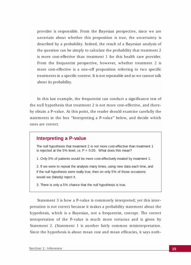
In this last example, the frequentist can conduct a significance test of

the null hypothesis that treatment 2 is not more cost-effective, and there-

by obtain a P-value. At this point, the reader should examine carefully the

statements in the box “Interpreting a P-value” below, and decide which

ones are correct.

Statement 3 is how a P-value is commonly interpreted; yet this inter-

pretation is not correct because it makes a probability statement about the

hypothesis, which is a Bayesian, not a frequentist, concept. The correct

interpretation of the P-value is much more tortuous and is given by

Statement 2. (Statement 1 is another fairly common misinterpretation.

Since the hypothesis is about mean cost and mean efficacies, it says noth-

Interpreting a P-value

The null hypothesis that treatment 2 is not more cost-effective than treatment 1is rejected at the 5% level, i.e. P = 0.05. What does this mean?

1. Only 5% of patients would be more cost-effectively treated by treatment 1.

2. If we were to repeat the analysis many times, using new data each time, and

if the null hypothesis were really true, then on only 5% of those occasions

would we (falsely) reject it.

3. There is only a 5% chance that the null hypothesis is true.

ing about individual patients.)

The primary reason why we cannot interpret a P-value in this way is

because it does not take account of how plausible the null hypothesis was a

priori.

Example.

An experiment is conducted to see whether thoughts can be transmit-

ted from one subject to another. Subject A is presented with a shuffled

deck of cards and tries to communicate to Subject B whether each card

is red or black by thought alone. In the experiment, Subject B correct-

ly gives the color of 33 cards. The null hypothesis is that no thought-

transference takes place and Subject B is randomly guessing. The

observation of 33 correct is significant with a (one-sided) P-value of

3.5%. Should we now believe that it is 96.5% certain that Subject A

can transmit her thoughts to Subject B?

Most scientists would regard thought-transference as highly implausi-

ble and in no way would be persuaded by a single, rather small, experi-

ment of this kind. After seeing this experimental result, most would still

strongly believe in the null hypothesis, regarding the outcome as due to

chance.

In practice, frequentist statisticians recognize that much stronger evi-

dence would be required to reject a highly plausible null hypothesis, such

as in the above example, than to reject a more doubtful null hypothesis.

This makes it clear that the P-value cannot mean the same thing in all sit-

uations and to interpret it as the probability of the null hypothesis is not

only wrong but could be seriously wrong when the hypothesis is a priori

highly plausible (or highly implausible).

To many users of statistics and even to many practicing statisticians, it

is perplexing that one cannot interpret a P-value as the probability that the

null hypothesis is true. Similarly, it is perplexing that one cannot interpret


a 95% confidence interval for a treatment difference as saying that the true

difference has a 95% chance of lying in this interval. Nevertheless, these

are wrong interpretations…and can be seriously wrong. The correct inter-

pretations are far more indirect and unintuitive. (See the Appendix for

more examples.)

Bayesian inferences have exactly the desired interpretations. A

Bayesian analysis of a hypothesis results precisely in the probability that it

is true. In addition, a Bayesian 95% interval for a parameter means pre-

cisely that there is a 95% probability that the parameter lies in that inter-

val. This is the essence of the key benefit (B1) – “more natural and inter-

pretable inferences” – offered by Bayesian methods.

Section 1: Inference 1717


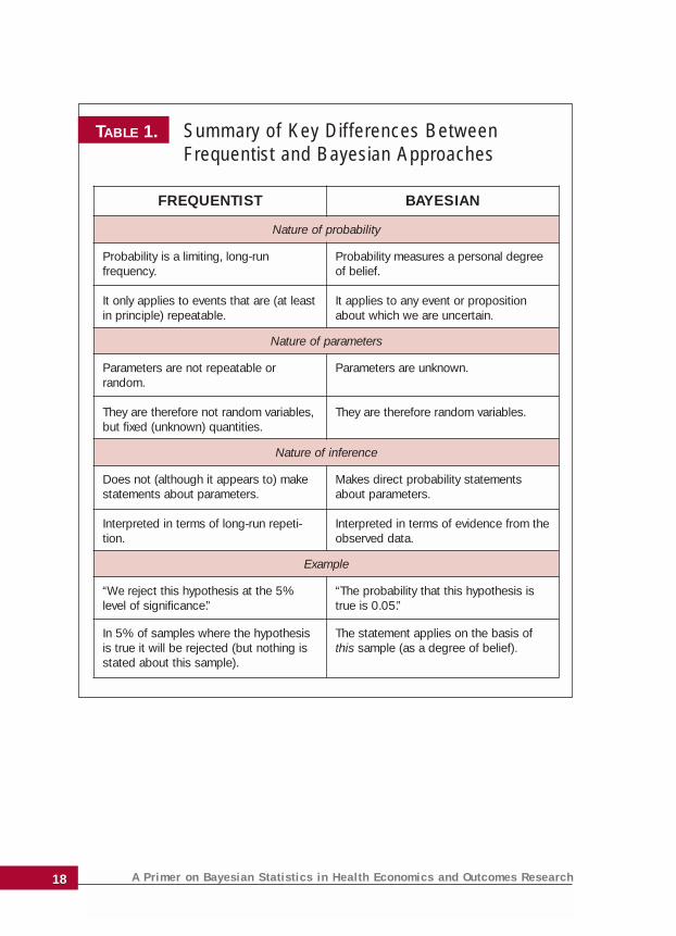
TABLE 1. Summary of Key Differences Between Frequentist and Bayesian Approaches

FREQUENTIST BAYESIAN

Nature of probability

Probability is a limiting, long-run frequency.

It only applies to events that are (at leastin principle) repeatable.

Probability measures a personal degreeof belief.

It applies to any event or propositionabout which we are uncertain.

Nature of parameters

Parameters are not repeatable or random.

They are therefore not random variables,but fixed (unknown) quantities.

Parameters are unknown.

They are therefore random variables.

Nature of inference

Does not (although it appears to) makestatements about parameters.

Interpreted in terms of long-run repeti-tion.

Makes direct probability statementsabout parameters.

Interpreted in terms of evidence from theobserved data.

Example

“We reject this hypothesis at the 5%level of significance.”

“The probability that this hypothesis istrue is 0.05.”

In 5% of samples where the hypothesisis true it will be rejected (but nothing isstated about this sample).

The statement applies on the basis ofthis sample (as a degree of belief).


SECTION 1SECTION 2

191919

The fundamentals of Bayesian statistics are very simple. The

Bayesian paradigm is one of learning from data.

The role of data is to add to our knowledge and so to update what

we can say about the parameters and relevant hypotheses. As such,

whenever we wish to learn from a new set of data, we need to iden-

tify what is known prior to observing those data. This is known as prior

information. It is through the incorporation of prior information that

the Bayesian approach utilizes more information than the frequentist

approach. A discussion of precisely what the prior information repre-

sents and where it comes from can be found in the next section: Prior

Information. For purposes of exposition of how the Bayesian paradigm

works, we simply suppose that the prior information has been identi-

fied and is expressed in the form of a prior distribution for the

unknown parameters of the statistical model. The prior distribution

expresses what is known (or believed to be true) before seeing the

new data. This information is then synthesized with the information

in the data to produce the posterior distribution, which expresses

what we now know about the parameters after seeing the data. (We

often refer to these distributions as ‘the prior’ and ‘the posterior’.)

The mathematical mechanism for this synthesis is Bayes’ theo-

rem, and this is why this approach to statistics is called “Bayesian”.

From a historical perspective, the name originated from the Reverend

The Bayesian MethodSECTION 2


Thomas Bayes, an 18th century minister who first showed the use of the

theorem in this way and gave rise to Bayesian statistics.

The process is simply illustrated in the box “Example of Bayes’

theorem”.

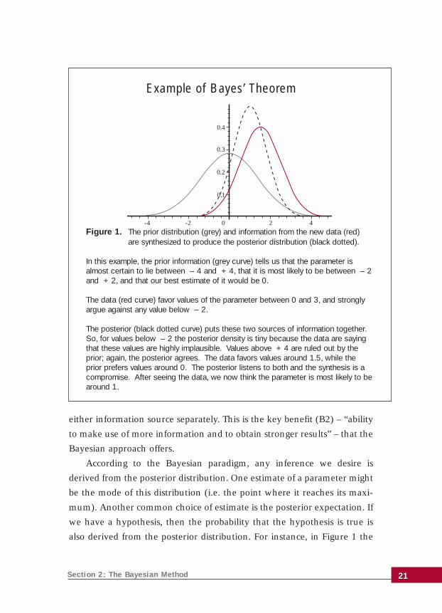
Figure 1 is called a triplot and is a way of seeing how Bayesian meth-

ods combine the two information sources. The strength of each source of

information is indicated by the narrowness of its curve – a narrower curve

rules out more parameter values and so represents stronger information.

In Figure 1, we see that the new data (red curve) are a little more inform-

ative than the prior (grey curve). Since Bayes’ theorem recognizes the

strength of each source, the posterior (black dotted curve) in Figure 1 is

influenced a little more by the data than by the prior. For instance, the pos-

terior peaks at 1.33, a little closer to the peak of the data curve than to the

prior peak. Notice that the posterior is narrower than either the prior or

the data curve, reflecting the way that the posterior has drawn strength

from both information sources.

The data curve is technically called the likelihood and is also important

in frequentist inference. Its role in both inference paradigms is to describe

the strength of support from the data for the various possible values of the

parameter. The most obvious difference between frequentist and Bayesian

methods is that frequentist statistics uses only the likelihood, whereas

Bayesian statistics uses both the likelihood and the prior information.

In Figure 1, the Bayesian analysis produces different inferences from

the frequentist approach because it uses the prior information as well as

the data. The frequentist estimate, using the data alone, is around 1.5. The

Bayesian analysis uses the fact that it is unlikely, on the basis of the prior

information, that the true parameter value is 2 or more. As a result, the

Bayesian estimate is around 1. The Bayesian analysis combines the prior

information and data information in a similar way to how a meta-analysis

combines information from several reported trials. The posterior estimate

is a compromise between prior and data estimates and is a more precise

estimate (as seen in the posterior density being a narrower curve) than

Section 2: The Bayesian Method 2121

either information source separately. This is the key benefit (B2) – “ability

to make use of more information and to obtain stronger results” – that the

Bayesian approach offers.

According to the Bayesian paradigm, any inference we desire is

derived from the posterior distribution. One estimate of a parameter might

be the mode of this distribution (i.e. the point where it reaches its maxi-

mum). Another common choice of estimate is the posterior expectation. If

we have a hypothesis, then the probability that the hypothesis is true is

also derived from the posterior distribution. For instance, in Figure 1 the

Figure 1. The prior distribution (grey) and information from the new data (red) are synthesized to produce the posterior distribution (black dotted).

In this example, the prior information (grey curve) tells us that the parameter isalmost certain to lie between – 4 and + 4, that it is most likely to be between – 2and + 2, and that our best estimate of it would be 0.

The data (red curve) favor values of the parameter between 0 and 3, and stronglyargue against any value below – 2.

The posterior (black dotted curve) puts these two sources of information together.So, for values below – 2 the posterior density is tiny because the data are sayingthat these values are highly implausible. Values above + 4 are ruled out by theprior; again, the posterior agrees. The data favors values around 1.5, while theprior prefers values around 0. The posterior listens to both and the synthesis is acompromise. After seeing the data, we now think the parameter is most likely to bearound 1.

Example of Bayes’ Theorem

0.1

0.2

0.3

0.4

-4 -2 0 2 4

probability that the parameter is positive is the area under the black dot-

ted curve to the right of the origin, which is 0.89.

In contrast to frequentist inference, which must phrase all questions in

terms of significance tests, confidence intervals and unbiased estimators,

Bayesian inference can use the posterior distribution very flexibly to pro-

vide relevant and direct answers to all kinds of questions. One example is

the natural link between Bayesian statistics and decision theory. By com-

bining the posterior distribution with a utility function (which measures

the consequences of different decisions), we can identify the optimal deci-

sion as that which maximizes the expected utility. In economic evaluation,

this could reduce to minimizing expected cost or to maximizing expected

efficacy, depending on the utility function. However, from the perspective

of cost-effectiveness, the most appropriate utility measure is net benefit

(defined as the mean efficacy times willingness to pay, minus expected

cost).

For example, consider a health care provider that has to choose which

of two procedures to reimburse. The optimal decision is to choose the one

that has the higher expected net benefit. A Bayesian analysis readily pro-

vides this answer, but there is no analogous frequentist analysis. To test the

hypothesis that one net benefit is higher than the other simply does not

address the question properly (in the same way that to compute the prob-

ability that the net benefit of procedure 2 is higher than that of procedure

1 is not the appropriate Bayesian answer). More details of this example

and of Bayes’ theorem can be found in the Appendix.

This serves to illustrate another key benefit of Bayesian statistics, (B4)

– “Bayesian methods are ideal for decision making”.



SECTION 1SECTION 3

232323

The prior information is both a strength and a potential weak-

ness of the Bayesian approach. We have seen how it allows

Bayesian methods to access more information and so to produce

stronger inferences. As such it is one of the key benefits of the

Bayesian approach. On the other hand, most of the criticism of

Bayesian analysis focuses on the prior information.

The most fundamental criticism is that prior information is sub-

jective: your prior information is different from mine, and so my prior

distribution is different from yours. This makes the posterior distribu-

tion, and all inferences derived from it, subjective. In this sense, it is

claimed that the whole Bayesian approach is subjective. Indeed,

Bayesian methods are based on a subjective interpretation of proba-

bility, which is described in Table 1 as a “personal degree of belief”. This

formulation is necessary (see the Appendix for details) if we are to give

probabilities to parameters and hypotheses, since the frequentist inter-

pretation of probability is too narrow. Yet for many scientists trained

to reject subjectivity whenever possible, this is too high a price to pay

for the benefits of Bayesian methods. To its critics, (D1) “subjectivity”

is the key drawback of the Bayesian approach.

We believe that this objection is unwarranted both in principle

and in practice. It is unwarranted in principle because science cannot

be truly objective. In practice it is unwarranted because the Bayesian

Prior InformationSECTION 3

method actually very closely reflects the real nature of the scientific

method, in the following respects:

Subjectivity in the prior distribution is minimized through basing prior

information on defensible evidence and reasoning.

Through the accumulation of data, differences in prior positions are

resolved and consensus is reached.

Taking the second of these points first, Bayes’ theorem weights the prior

information and data according to their relative strengths in order to derive

the posterior distribution. If prior information is vague and insubstantial

then it will get negligible weight in the synthesis with the data, and the pos-

terior will in effect be based entirely on data information (as expressed in the

likelihood function). Similarly, as we acquire more and more data, the

weight that Bayes’ theorem attaches to the newly acquired data relative to

the prior increases. Again, the posterior is effectively based entirely on the

information in the data. This feature of Bayes’ theorem mirrors the process

of science, where the accumulation of objective evidence is the primary

process whereby differences of opinion are resolved. Once the data provide

conclusive evidence, there is essentially no room left for subjective opinion.

Returning to the first point above, it is stated that where genuine, sub-

stantial prior information exists it needs to be based on defensible evidence

and reasoning. This is clearly important when the new data are not so

extensive as to overwhelm the prior information, so that Bayes’ theorem

will give the prior a non-negligible weight in its synthesis with the data.

Prior information of this kind exists routinely in medical applications, and

in particular in economic evaluation of competing technologies.

Two examples are presented in the Appendix. One concerns the analy-

sis of subgroup differences, where prior skepticism about the existence of

such effects without a plausible biological mechanism is naturally accom-

modated in the Bayesian analysis.

The other example concerns a case where a decision on the cost-effec-

tiveness of a new drug versus standard treatment depends in large part on

evidence about hospitalizations. A small trial produces an apparently large

A Primer on Bayesian Statistics in Health Economics and Outcomes Research 2424

(and, in frequentist terms, significant) reduction in mean days in hospital.

However, an earlier and much larger trial produced a much less favorable

estimate of mean hospital days for a similar drug. There are two possible

responses that a frequentist analysis can have to the earlier trial:

1. Take the view that there is no reason why the hospitalization rate

under the old drug should be the same as under the new one, in which

case the earlier trial is ignored because it contributes no information

about the new drug.

2. Take the view that the two drugs should have essentially identical

hospitalization rates – and so we pool the data from the two trials.

The second option will lead to the new data being swamped by the

much larger earlier trial, which seems unreasonable, but the first option

entails throwing away potentially useful information. In practice, a fre-

quentist would probably take the first option, but with a caveat that the

earlier trial suggests this may underestimate the true rate.

It would usually be more realistic to take the view that the two hospital-

ization rates will be different but similar. The Appendix demonstrates how a

Bayesian analysis can accommodate the earlier trial as prior information

although it necessitates a judgement about similarity of the drugs. How dif-

ferent might we have believed their hospitalization rates to be before con-

ducting the new trial?

The Bayesian analysis produces a definite and quantitative synthesis of

the two sources of information rather than just the vague “an earlier trial on

a similar drug produced a higher mean days in hospital, and so I am skepti-

cal about the reduction seen in this trial”. This synthesis results from making

a clear, reasoned and transparent interpretation of the prior information.

This is part of the key benefit (B5) – “more transparent judgements” – of the

Bayesian approach. Without the Bayesian analysis it would be natural to

moderate the claims of the new trial. The extent of such moderation would

still be judgmental, but the judgement would not be so open and the result

would not be transparently derived from the judgement by Bayes’ theorem.

Section 3: Prior Information 2525

This leads to another important way in which Bayesian methods are

transparent. Once the prior distribution and likelihood have been formu-

lated (and openly laid on the table), the computation of the posterior dis-

tribution and the derivation of appropriate posterior inferences or deci-

sions are uniquely determined. In contrast, once the likelihood has been

determined in a frequentist analysis there is still the freedom to choose

which of many inference rules to apply. For instance, although in simple

problems it is possible to identify optimal estimators, in general, there are

likely to be many unbiased estimators – none of which dominates any of

the others in the sense of having uniformly smaller variance. The practi-

tioner is then free to use any of these or to dream up others on an “ad hoc”

basis. This feature of frequentism leads to a lack of transparency because

the respective choices are, in essence, arbitrary.

So what of the criticism (D1), that Bayesian methods are inherently sub-

jective? It is true that one could carry out a Bayesian analysis with a prior

distribution based on mere guesswork, prejudice or wishful thinking. Bayes’

theorem technically admits all of these unfortunate practices, but Bayesian

statistics does not in any sense condone them. Also, recall that in a proper

Bayesian analysis, prior information is not only transparent but is also based

on both defensible evidence and reasoning which, if followed, will lead any

above-mentioned abuses to become transparent, and so to be rejected.

A compact statement of what should constitute prior information is

provided in the box ‘The Evidence’.


The ‘Evidence’

Prior information should be based on sound evidence and reasoned judgements. A good way to think of this is to parody a familiar quotation: the prior distributionshould be ‘the evidence, the whole evidence and nothing but the evidence’:

• ‘the evidence’ – genuine information legitimately interpreted;• ‘the whole evidence’ – not omitting relevant information (preferably a

consensus that pools the knowledge of a range of experts);• ‘nothing but the evidence’ – not contaminated by bias or prejudice.


SECTION 1SECTION 4

272727

We hope that the preceding sections convince the reader that

prior information exists and should be used, in as rea-

soned, objective and fully transparent a way as possible. Here we

address the question of how to formulate a prior probability distribu-

tion, the grey curve in Figure 1.

Refer to the example in the previous section where prior infor-

mation consists of information about hospitalization in a trial of a sim-

ilar drug. In the Appendix this is formulated as a prior distribution

with mean 0.21 (average days in hospital per patient) and standard

deviation 0.08. This is justified by reference to the trial in question,

where the average days in hospital under the different but similar drug

was estimated to be 0.21 with a standard error of 0.03. But how is the

stated prior distribution obtained from the given prior information?

Judgement inevitably intervenes in the process of specifying the

prior distribution. As in the above case, it typically arises through the

need to interpret the prior information and its relevance to the new

data. How different might the hospitalization rates be under the two

drugs? Different experts may interpret the prior information different-

ly. As well, a given expert may interpret the information differently at

a later time, such as in the example of deciding on a prior standard

deviation of 0.75 rather than 0.8.

Prior SpecificationSECTION 4

Even though our prior information might be genuine evidence with a

clear relation to the new data, we cannot convert this into a prior distri-

bution with perfect precision and reliability. This is the drawback (D2) –

“prior specification is unreliable”.

Nevertheless, in practice we only need to specify the prior distribution

with sufficient reliability and accuracy. We can explore the range of plau-

sible prior specifications based on reasonable interpretations of the evi-

dence and allowing for imprecision in the necessary judgements. If the

posterior inferences or decisions are essentially insensitive to those varia-

tions, then the inherent unreliability of the prior specification process does

not matter. This practice of sensitivity analysis with respect to the prior

specification is a basic feature of practical Bayesian methodology as it is in

all decision analysis applications.

The precision needed in the prior specification to achieve robust infer-

ences and decisions depends on the strength of the new data. As we have

seen, given strong enough data, the prior information matters little or not

at all and differences of judgement in interpreting the data will be unim-

portant. When the new data are not so strong, and prior information is

appreciable, then sensitivity analysis is essential. It is also important to note

that, despite obvious drawbacks, expert opinion is sometimes quite a use-


Types and definitions of prior distribution

Informative (or genuine) priors: represent genuine prior information and bestjudgement of its strength and relation to the new data.

Noninformative (or default, reference, improper, weak, ignorance) priors:represent complete lack of credible prior information.

Skeptical priors: supposed to represent a position that a null hypothesis is likelyto be true.

Structural (or hierarchical) priors: incorporate genuine prior information aboutrelationships between parameters.

ful component of prior information. The procedures to elicit expert judge-

ments are an active topic of research by both statisticians and psychologists.

Up until now, we have been considering genuine informative prior

distributions. Some other ways to specify the prior distribution in a

Bayesian analysis are set out in the box, “Types and definitions of prior

distribution”.

In response to the difficulty of accurately and reliably eliciting prior

distributions, some have proposed conventional solutions that are sup-

posed to represent either no prior beliefs or a skeptical prior position.

The argument in favor of representing no prior information is that this

avoids any criticism about subjectivity. There have been numerous

attempts to find a formula for representing prior ignorance, but without

any consensus. Indeed, it is almost certainly an impossible quest.

Nevertheless, the various representations that have been derived can be

useful – at least for representing relatively weak prior information.

When the new data are strong (relative to the prior information), the

prior information is not expected to make any appreciable contribution to

the posterior. In this situation, it is pointless (and not cost-effective) to

spend much effort on carefully eliciting the available prior information.

Instead, it is common in such a case to apply some conventional ‘nonin-

formative’, ‘default’, ‘reference’, ‘improper’, ‘vague’, ‘weak’ or ‘ignorance’

prior (although the last of these is really a misnomer). These terms are

used more or less interchangeably in Bayesian statistics to denote a prior

distribution representing very weak prior information. The term ‘improp-

er’ is used because technically most of these distributions do not actually

exist in the sense that a normal distribution with an infinite variance does

not exist.

The idea of using so-called ‘skeptical’ priors is that if a skeptic can be

persuaded by the data then anyone with a less skeptical prior position

would also be persuaded. Thus, if one begins with a skeptical prior position

with regard to some hypothesis and is nevertheless persuaded by the data,

so that their posterior probability for that hypothesis is high, then some-

Section 4: Prior Specification 2929

one else with a less skeptical prior position would end up giving that

hypothesis an even higher posterior probability. In that case, the data are

strong enough to reach a firm conclusion. If, on the other hand, when we

use a skeptical prior the data are not strong enough to yield a high poste-

rior probability for that hypothesis, then we should not yet claim any def-

inite inference about it. Although this is another tempting idea, there is

even less agreement or understanding about what a skeptical prior should

look like.

The rather more complex ideas of structural or hierarchical priors (the

last category in the box “Types and definitions of prior distribution”) are

discussed in the Appendix.



SECTION 1SECTION 5

313131

Software is essential for any but the simplest of statistical tech-

niques, and Bayesian methods are no exception. In Bayesian

statistics, the key operations are to implement Bayes’ theorem and

then to derive relevant inferences or decisions from the posterior dis-

tribution. In very simple problems these tasks can be done algebraical-

ly, but this is not possible in even moderately complex problems.

Until the 1990s, Bayesian methods were interesting, but they found

little practical application because the necessary computational tools and

software had not been developed. Anyone who wanted to do serious

statistical analysis had no alternative but to use frequentist methods. In

little over a decade that position has been dramatically turned around.

Computing tools were developed specifically for Bayesian analysis that

are more powerful than anything available for frequentist methods in

the sense that Bayesians can now tackle enormously intricate problems

that frequentist methods cannot begin to address. It is still true that

Bayesian methods are more complex and that, although the computa-

tional techniques are well understood in academic circles, there is still a

lack of user-friendly software for the general practitioner.

The transformation is continuing, and computational develop-

ments are shifting the balance between the drawback (D3) – “com-

plexity and lack of software” – and the benefit (B3) – “ability to tack-

le more complex problems”. The main tool is a simulation technique

ComputationSECTION 5

called Markov chain Monte Carlo (MCMC). The idea of MCMC is in a sense

to bypass the mathematical operations rather than to implement them.

Bayesian inference is solved by randomly drawing a very large simulated

sample from the posterior distribution. The point is that if we have a suf-

ficiently large sample from any distribution then we effectively have that

whole distribution in front of us. Anything we want to know about the dis-

tribution we can calculate from the sample. For instance, if we wish to

know the posterior mean we just calculate the mean of this ‘inferential

sample’. If the sample is big enough, the sample mean is an extremely

accurate approximation to the true distribution mean, such that we can

ignore any discrepancy between the two.

The availability of computational techniques like MCMC makes exact

Bayesian inferences possible even in very complex models. Generalized

linear models, for example, can be analyzed exactly by Bayesian methods,

whereas frequentist methods rely on approximations. In fact, Bayesian

modelling in seriously complex problems freely combines components of

different sorts of modelling approaches with structural prior information,

unconstrained by whether such model combinations have ever been stud-

ied or analyzed before. The statistician is free to model the data and other

available information in whatever way seems most realistic. No matter

how messy the resulting model, the posterior inferences can be computed

(in principle, at least) by MCMC.

Bayesian methods have become the only feasible tools in several

fields such as image analysis, spatial epidemiology and genetic pedigree

analysis.

Although there is a growing range of software available to assist with

Bayesian analysis, much of it is still quite specialized and not very useful

for the average analyst. Unfortunately, there is nothing available yet that

is both powerful and user-friendly in the way that most people expect sta-

tistical packages to be. Two software packages that are in general use, freely


available and worth mentioning are First Bayes and WinBUGS.

First Bayes is a very simple program that is aimed at helping the begin-

ner learn and understand how Bayesian methods work. It is not intend-

ed for serious analysis of data, nor does it claim to teach Bayesian sta-

tistics, but it is in use in several universities worldwide to support cours-

es in Bayesian statistics. First Bayes can be very useful in conjunction

with a textbook – such as those recommended in the Further Reading

section of this Primer – and can be freely downloaded from

http://www.shef.ac.uk/~st1ao/.

WinBUGS is a powerful program for carrying out MCMC computations

and is in widespread use for serious Bayesian analysis. WinBUGS has been

a major contributing factor to the growth of Bayesian applications and can

be freely downloaded from http://www.mrc-bsu.cam.ac.uk/bugs/. Please

note, however, that WinBUGS is currently not very user-friendly and

sometimes crashes with inexplicable error messages. Given the growing

popularity of Bayesian methods, it is likely that more robust, user-friendly

commercial software will emerge in the coming years.

The Appendix provides more detail on these two sides of the Bayesian

computing coin: the drawback (D3) – “complexity and lack of software” –

and the benefit (B3) – “ability to tackle more complex problems”.

Section 5: Computation 3333


SECTION 1SECTION 6

353535

Bayesian techniques are inherently useful for designing clinical

trials because trials tend to be sequential, each designed based

in large part on prior trial evidence. The substantial literature that is

available regarding clinical trial design using Bayesian techniques is, of

course, applicable to design of cost-effectiveness trials.

By their nature, cost-effectiveness trials always have prior clinical

and probably some form of economic information, which in the fre-

quentist approach would be used to set the power requirements for

the trial, and hence to identify the sample size. Since the prior infor-

mation is explicitly stated in Bayesian design techniques, the depend-

ence of the chosen design on prior information is fully transparent. A

Bayesian analysis would formulate prior knowledge about how large

an effect might be achieved. For instance, in planning a Phase III trial

there will be information from Phase II studies on which to base a

prior distribution for the effect. This permits an informative approach

to setting sample size.

For a given sample size, the Bayesian calculation computes the

probability that the trial will successfully demonstrate a positive effect

(see O’Hagan and Stevens, 2001b). This can then be directly linked to

a decision about whether a trial of a certain size (and hence cost), with

this assurance of success (and consequent financial return), is worth-

Design and Analysis of Trials

SECTION 6

while. This contrasts with the frequentist power calculations, which only

provide a probability of demonstrating an effect conditional on the

unknown true effect taking some specific value.

An important simplifying feature of Bayesian design is that interim

analyses can be introduced without affecting the final conclusions, and

they do not need to be planned in advance. This is because Bayesian analy-

sis does not suffer from the paradox of frequentist interim analysis, that

two sponsors running identical trials and obtaining identical results may

reach different conclusions if one performs an interim analysis (but does

not stop the trial then) and the other does not. A Bayesian trial can be

stopped early or extended for any appropriate reason without needing to

compensate for such actions in subsequent analysis.

Aside from designing trials, a Bayesian approach is also useful for ana-

lyzing trial results. Today we see a growing interest in economic evaluation

that has led to inclusion of cost-effectiveness as a secondary objective in

traditional clinical trials. This may simply mean the collection of some

resource use data alongside conventional efficacy trials, but may extend to

more comprehensive economic data, more pragmatic enrollment, more

relevant outcome measures and/or utilities. Methods of statistical analysis

have begun to be developed for such trials. A useful review of Bayesian

work in this area is O’Hagan and Stevens (2002).

Early statistical work concentrated on deriving inference for the incre-

mental cost-effectiveness ratio, but the peculiar properties of ratios result-

ed in less than optimal solutions for various reasons. More recently, inter-

est has focused on inference for the (incremental) net benefit, which is

more straightforward statistically. Bayesian analyses have almost exclu-

sively adopted the net benefit approach. In fact, when using net benefits

the most natural expression of the relative cost-effectiveness of two treat-

ments is the cost-effectiveness acceptability curve (van Hout et al, 1994);

the essentially Bayesian nature of this measure is discussed in the

Appendix.


Costs in trials, as everywhere, are invariably highly skewed. Bayesian

methods accommodate this feature easily. O’Hagan and Stevens (2001a)

provide a good example where the efficacy outcome is binary. They model

costs as lognormally distributed (so explicitly accommodating skewness)

and allow different lognormal distributions for patients who have positive

or negative efficacy outcomes in each treatment group. They also illustrate

how even simple structural prior information can help provide more real-

istic posterior inferences in a dataset where two very high cost patients

arise in one patient group. Such a model is straightforwardly analyzed by

MCMC. Stevens et al (2003) provide full details of WinBUGS code to com-

pute posterior inferences. Another good example is Sutton et al (2003).

Section 6: Design and Analysis of Trials 3737


SECTION 1SECTION 7

393939

Economic evaluation is widely practiced by building economic

models (Chilcott et al, 2003). Even when cost-related data have

been collected alongside efficacy in a clinical trial, they will rarely be

adequate for a proper economic evaluation. This is because, as is wide-

ly understood, practice patterns within clinical trials differ radically

from practice patterns in community medicine (the latter being the

context of practical interest). More realistically, such data will inform

some of the inputs (e.g. clinical efficacy data) to the cost-effectiveness

model, while other input values (e.g. resource use, prices) will be

derived from other sources.

Inputs to economic models can at best only be estimates of the

unknown true values of these parameters – a fact that is recognized in

the practice of performing sensitivity analysis. Often, this consists of a

perfunctory one-way sensitivity analysis in which one input at a time

is varied to some ad hoc alternative value and the model rerun to see

if the cost-effectiveness conclusion changes. Even when none of these

changes in single parameter values is enough to change the conclusion

as to which treatment is more cost-effective, the analysis gives no quan-

tification of the confidence we can attach to this being the correct infer-

ence. The true values of individual inputs might be outside the ranges

explored. Furthermore, if two or more inputs are varied together with-

in those ranges they might change the conclusion.

Economic ModelsSECTION 7

The statistically sound way to assess the uncertainty in the model out-

put that arises from uncertainty in its inputs is probabilistic sensitivity

analysis (PSA). This is the approach that is recommended by NICE, other

statutory agencies and many academic texts. It consists of assigning proba-

bility distributions to the inputs, so as to represent the uncertainty we have

in their true values, and then propagating this uncertainty through the

model. There is increasing awareness of the benefits of PSA; two examples

are Briggs et al (2002) and Parmigiani (2002).

It is important to appreciate that in PSA we are putting probability dis-

tributions on unknown parameters, which makes it unequivocally a

Bayesian analysis. In effect, Bayesian methods have been widely used in

health economics for years. The recognition of the Bayesian nature of these

probability distributions has important consequences. The distributions

should be specified using the ideas discussed in Section 4, Prior Specification.

In particular, the evidence sought to populate economic models rarely relates

directly to the parameters that the model actually requires in any applica-

tion. Trial data will be from a different population (possibly in a different

country) and with different compliance, registry data are potentially biased

and so forth. Just as we considered with the use of prior information in gen-

eral Bayesian analyses, the relationship between the data used to populate

the model and the parameters that define the use we wish to make of the

model is a matter for judgement. It is common to ignore these differences.

However, using the estimates and standard errors reported in the literature

as defining the input distributions will under-represent the true uncertainty.

The usual technique for PSA is Monte Carlo simulation, in which random

sets of input values are drawn and the model run for each set. This gives a sam-

ple from the output distribution (which is very similar to MCMC sampling

from the posterior distribution). This is feasible when the model is simple

enough to run almost instantaneously on a computer but for more complex

models it may be impractical to obtain a sufficiently large sample of runs. For

such situations, Stephenson et al (2002) describe an alternative technique,

based on Bayesian statistics, for computing the output distribution using far

fewer model runs.


Once the uncertainty in the model output has been quantified in PSA

by its probability distribution, the natural way to express uncertainty about

cost-effectiveness is again through the cost-effectiveness acceptability curve.

As mentioned already, this is another intrinsically Bayesian construction.

A natural response to uncertainty about cost-effectiveness is to ask

whether obtaining further data might reduce uncertainty. In the United

Kingdom, for instance, one of the decisions that NICE might make when asked

to decide on cost-effectiveness of a drug is to say that there is insufficient evi-

dence at present, and defer approving the drug for reimbursement by the

National Health Service until more data have been obtained. Bayesian decision

theory provides a conceptually straightforward way to inform such a deci-

sion, through the computation of the expected value of sample information.

Expected value of information calculations have been advocated by Felli

and Hazen (1998), Claxton and Posnett (1996), Brennan et al (2003) and a

Bayesian calculation for complex models developed by Oakley (2002). There

is a strong link between such analyses and design of trials, since balancing

the expected value of sample information against sampling costs is a stan-

dard Bayesian technique for identifying an optimal sample size.

There is another important link between the analysis of economic mod-

els and the analysis of cost-effectiveness trials. Where the evidence for indi-

vidual parameters in an economic model comes from a trial or other statisti-

cal data, the natural distribution to assign to those parameters is their poste-

rior distribution from a fully Bayesian analysis of the raw data. This assumes

that the data are directly relevant to the parameter required in the model,

rather than relating strictly to a similar, but different, parameter. In the lat-

ter case, it is simple to link the posterior distribution from the data analysis

to the parameters needed for the model, using structural prior information.

This linking of statistical analysis of trial data to economic model inputs

is a form of evidence synthesis and illustrates the holistic nature of the

Bayesian approach. Examples are given by Ades and Lu (2002) and Cooper

et al (2002). Ades et al synthesize evidence from a range of overlapping data

sources within a single Bayesian analysis. Synthesizing evidence is exactly

what Bayes’ theorem does.

4141Section 7: Economic Models

In this section we will briefly summarize the main messages being con-

veyed in this Primer.

• Bayesian methods are different from and, we posit, have certain

advantages over conventional frequentist methods, as set out in

benefits (B1) to (B5) of the Overview. These benefits are explored and

illustrated in various ways throughout subsequent sections of the

Primer.

• There are some perceived disadvantages of Bayesian methods, as set

out in the drawbacks (D1) to (D3) in the Overview. These are also

discussed in subsequent sections and we describe how they are

being addressed. It is up to the reader to judge the degree to which

the benefits may outweigh the drawbacks in practice.

• Bayesian technologies have already been developed in many of the

key methodologies of health economics. Already we see clear

advantages in the design and analysis of cost-effectiveness trials,

quantification of uncertainty in economic models, expression of

uncertainty about cost-effectiveness, assessment of the value of

potential new evidence, and synthesis of information going into

and through an economic evaluation.

• There is enormous scope for the development of new and more

sophisticated Bayesian techniques in health economics and out-

comes research. We are confident that Bayesian analysis will

increasingly become the approach of choice for the development

and evaluation of submissions on cost-effectiveness of medical

technologies, as well as for pure cost or utility studies.


Conclusions


Articles and books cited in the text (including those in the

Appendix) are listed below. This is by no means an exhaustive list of

Bayesian work in the field. Suggestions for further reading are given at

the end.

Ades, A. E. and Lu, G. (2002). Correlations between parameters in riskmodels: estimation and propagation of uncertainty by Markov ChainMonte Carlo. Technical report, MRC Health Services ResearchCollaboration, University of Bristol.

Brennan, A., Chilcott, J., Kharroubi, S. A. and O’Hagan, A. (2003).Calculating expected value of perfect information – resolution of the uncer-tainty in methods and a two level Monte Carlo approach. Technical report,School of Health and Related Research, University of Sheffield.

Briggs, A. H., Goeree, R., Blackhouse, G. and O’Brien, B. J. (2002).Probabilistic analysis of cost-effectiveness models: choosing between treat-ment strategies for gastroesophageal reflux disease. Medical Decision Making22, 290-308.

Chilcott, J. Brennan, A., Booth, A., Karnon, J. and Tappenden, P. (2003).The role of modelling in the planning and prioritisation of clinical trials. Toappear in Health Technology Assessment.

Claxton, K. (1999). The irrelevance of inference: a decision-makingapproach to the stochastic evaluation of health care technologies. Journal ofHealth Economics 18, 341-364.

Bibliography andFurther Reading

434343

Claxton, K. and Posnett, J. (1996). An economic approach to clinical trial designand research priority-setting. Health Economics 5, 513-524.

Cooke, R. M. (1991). Experts in Uncertainty: Opinion and Subjective Probability inScience. Oxford: Oxford University Press.

Cooper, N. J., Sutton, A. J., Abrams, K. R. (2002). Decision analytical econom-ic modelling within a Bayesian framework: application to prophylactic antibi-otics use for caesarean section. Statistical Methods in Medical Research 11, 491-512.

Felli, C. and Hazen, G. B. (1998). Sensitivity analysis and the expected value ofperfect information. Medical Decision Making 18, 95-109.

Kadane, J. B. and Wolfson, L. J. (1998). Experiences in elicitation. TheStatistician 47, 1-20.

Lichtenstein, S., Fischhoff, B. and Phillips, L. D. (1982). Calibration of probabil-ities: the state of the art to 1980. In Judgement Under Uncertainty: Heuristics andBiases, D. Kahneman, P. Slovic. and A. Tversky (Eds.) Cambridge UniversityPress: Cambridge, pp. 306-334.

Löthgren, M. and Zethraeus, N. (2000). Definition, interpretation and calcula-tion of cost-effectiveness acceptability curves. Health Economics 9, 623-630.

Meyer, M. and Booker, J. (1981). Eliciting and Analyzing Expert Judgement: APractical Guide, volume 5 of “Knowledge-Based Expert Systems”. AcademicPress.

Oakley J. (2002). Value of information for complex cost-effectiveness models.Research Report No. 533/02, Department of Probability and Statistics,University of Sheffield.

O’Hagan, A. and Stevens, J. W. (2001a). A framework for cost-effectivenessanalysis from clinical trial data. Health Economics 10, 302-315.

O’Hagan, A. and Stevens, J. W. (2001b). Bayesian assessment of sample size forclinical trials of cost-effectiveness. Medical Decision Making 21, 219-230.

O’Hagan, A. and Stevens, J. W. (2002). Bayesian methods for design and analy-sis of cost-effectiveness trials in the evaluation of health care technologies.Statistical Methods in Medical Research 11, 469-490.


O’Hagan, A., Stevens, J. W. and Montmartin, J. (2000). Inference for the cost-effectiveness acceptability curve and cost-effectiveness ratio. PharmacoEconomics17, 339-349.

Parmigiani, G. (2002). Measuring uncertainty in complex decision analysismodels. Statistical Methods in Medical Research 11, 513-537.

Stevens, J. W., O’Hagan, A. and Miller, P. (2003). Case study in the Bayesiananalysis of a cost-effectiveness trial in the evaluation of health care technolo-gies: Depression. Pharmaceutical Statistics 2, 51-68.

Stevenson, M. D., Oakley, J. and Chilcott, J. B. (2002). Gaussian process mod-elling in conjunction with individual patient simulation modelling. A case studydescribing the calculation of cost-effectiveness ratios for the treatment of osteo-porosis. Technical report, School of Health and Related Research, University ofSheffield.

Sutton, A. J., Lambert, P. C., Billingham, L., Cooper, N. J. and Abrams, K. R.(2003). Establishing cost-effectiveness with partially missing cost components.Technical report, Department of Epidemiology and Public Health, University ofLeicester.

Thisted. R. A. (1988). Elements of Statistical Computing. Chapman and Hall; NewYork.

Van Hout, B. A., Al, M. J., Gordon, G. S. and Rutten, F. (1994). Costs, effectsand C/E ratios alongside a clinical trial. Health Economics 3, 309-319.

Further reading on Bayesian statistics

Preparatory books. These books cover basic ideas of decision-theory and personal probability.Neither book assumes knowledge of mathematics above a very elementarylevel.

Lindley, D.V. (1980). Making Decisions, 2nd ed. Wiley, New York.

O’Hagan, A. (1988). Probability: Methods and Measurement. Chapman and Hall,London.

Bibliography and Further Reading 4545

Introductory books. Berry’s book is completely elementary. Lee’s book is aimed at undergraduatemathematics level.

Berry, D.A. (1996). Statistics: A Bayesian Perspective. Duxbury, London.

Lee, P.M. (1997). Bayesian Statistics: An Introduction, 2nd ed., Arnold, London.

More advanced texts.At an intermediate level, Migon and Gamerman is a nice, readable but concisebook. Congdon concentrates on how to develop models and computations forthe practical application of Bayesian methods. The last two books, by Bernardo& Smith, and by O’Hagan, are the most advanced, for people wishing to learnBayesian statistics in depth.

Migon, H. S. and Gamerman, D. (1999). Statistical Inference: An IntegratedApproach. Arnold, London.

Congdon, P. (2001). Bayesian Statistical Modelling. John Wiley.

Bernardo, J. M. and Smith, A. F. M. (1994). Bayesian Theory. Wiley, New York.

O’Hagan, A. (1994). Bayesian Inference, volume 2B of “Kendall’s AdvancedTheory of Statistics”. Arnold, London.

PhilosophyFinally, the following presents the case for Bayesian inference from the per-spective of philosophers of science.

Howson, C. and Urbach, P. (1993). Scientific Reasoning, 2nd edition. Open Court;Peru, Illinois.



This Appendix offers more detailed discussion of the issues raised in the

first four sections of this Primer.

Inference – DetailsThe following subsections give details of the arguments presented in the

“Inference” section and of the key differences between Bayesian and frequentist

statistics identified in Table 1.

The nature of parameters

The most fundamental distinction between the Bayesian and frequentist

approaches is that in the Bayesian approach the unknown parameters in a sta-

tistical model are random variables. Accordingly, in a Bayesian analysis the

parameters have probability distributions, whereas in frequentist analysis they

are fixed but unknown quantities, and it is not permitted to make probability

statements about them.

This can be puzzling to the layman because a standard frequentist state-

ment like a confidence interval certainly seems to be making probability state-

ments about the unknown parameter. If we see the statement that [3.5, 11.6]

is a 95% confidence interval for a parameter µ, surely this is saying that there

is a 95% chance that µ lies between 3.5 and 11.6. No, it cannot mean this

because µ is not a random quantity in frequentist inference. We shall see what

it does mean when we discuss The nature of inferences.

In Bayesian statistics, the parameters do have probability distributions, and

if a Bayesian analysis produces a 95% interval then it does have exactly the

interpretation that is usually put on a confidence interval.

Appendix

The nature of probability

Underlying this distinction between the two approaches to statistics over the

nature of parameters is a difference in how they interpret probability itself. In fre-

quentist statistics, a probability can only be a long-run, limiting, relative frequen-

cy. This is the familiar definition used in elementary courses, often motivated by

ideas like tossing coins a very large number of times and looking at the long-run,

limiting frequency of ‘heads’. It is because it is based firmly on this frequency def-

inition of probability that we call those traditional methods ‘frequentist’. Bayesian

statistics, in contrast, rest on an interpretation of probability as a personal degree

of belief. Although to some this may seem ‘woolly’ and unscientific, it is impor-

tant to recognize that Bayesian statisticians have widely and successfully devel-

oped analyses based on this interpretation. As explained in Prior Information, it

does not lead to unbridled subjectivity and unscientific practices.

The necessity of such an interpretation becomes clearer when we appreci-

ate how many events that we would be willing to consider having probabilities

could never have a frequentist probability. The probability of a hypothesis is an

obvious example, since a particular hypothesis either is or is not true, and we

cannot consider any experimental repetitions of it like we could for tossing a

coin. Some other examples are the probability of rain tomorrow or the proba-

bility that you will experience a myocardial infarction (MI) during your life-

time. Tomorrow is a unique day, with meteorological conditions preceding it

today that have not existed in precisely the same form before, and never will

again, and you are a unique person whose genetic makeup and lifestyle make

you more or less disposed to MI at some point in your life in a way not precisely

matched by anyone else. Despite their uniqueness, we generally have no diffi-

culty in thinking of these events as having probabilities. Most of the uncertain

events and variables of real interest to scientists and practitioners are one-off

things, and the frequency interpretation of probability is completely unable to

accommodate our wish to describe them by probabilities.

The nature of inferences

Probabilities in the frequentist approach must be based on repetition. The

statement that [3.5, 11.6] is a 95% confidence interval for a parameter µ says


that if we repeated this experiment a great many times, and if we calculated an

interval each time using the rule we used this time to get the interval [3.5,

11.6], then 95% of those intervals would contain µ. The 95% probability is a

property of the rule that was used to create the interval, not of the interval

itself. It is simply not allowed, and would be wrong to attribute that probabili-

ty to the actual interval [3.5, 11.6]. This is a very unintuitive argument.

Frequentist statements such as these are widely misinterpreted, even by trained

statisticians. The erroneous interpretation of the confidence interval, that there

is a 95% chance of the parameter µ lying in the particular interval [3.5, 11.6],

is almost universally made by statistician and non-statistician alike.

Nevertheless, it is incorrect. A Bayesian interval, however, does have that inter-

pretation.

The Bayesian approach uses different terminology from the familiar fre-

quentist terms. Bayesian intervals are generally called credible intervals to make it

clear that they are different from confidence intervals. The highest density interval

is a credible interval with the property of being shortest among all available cred-

ible intervals with a given probability of containing the parameter’s true value.

An entirely similar argument can be made about frequentist significance

tests. If a hypothesis is rejected with a P-value of 1%, this does not mean that

the hypothesis has only a 1% probability of being true. Hypotheses do not have

probabilities in a frequentist analysis any more than parameters do. The P-value

must again be based on repetition of a rule. In this case it is a rule which says

that when the data satisfy some condition we will formally reject the hypothe-

sis. The P-value’s proper interpretation is that if we repeated the experiment

many times, and if the hypothesis really were true every time, then on only 1%

of such experiments would the rule lead us to (wrongly) reject that hypothesis.

This is a tricky and convoluted idea. It is not surprising that practitioners regu-

larly misinterpret a P-value as the probability that the hypothesis is true.

To interpret a P-value in this way is not only wrong but also dangerously

wrong. The danger arises because this interpretation ignores how plausible the

hypothesis might have been in the first place. Here are three examples.

Appendix 4949

Examples.

1) Screening. Consider a screening test for a rare disease. The test is very

accurate, with false-positive and false-negative rates of 0.1% (i.e. only

one person in a thousand who does not have the disease will give a

positive result, and only one person in a thousand with the disease will

give a negative result). You take the screen and your result is positive.

What should you think? Since the screen only makes one mistake in

a thousand, doesn’t this mean you are 99.9% certain to have the dis-

ease? In hypothesis testing terms, the positive result would allow you

to reject the null hypothesis that you don’t have the disease at the

0.1% level of significance, a highly significant result agreeing with that

99.9% diagnosis. But the disease is rare, and in practice we know that

most positives reporting for further tests will be false positives. If only

one person in 50,000 has this disease, your probability of having it

after a positive screening test is less than 1 in 50.

Although this example may not be obviously concerned with hypoth-

esis testing, in fact there is a direct analogy. We can consider using the

observation of a positive screening outcome as data with which to test

the null hypothesis that you do not have the disease. If the null

hypothesis is true, then the observation is extremely unlikely, and we

could formally reject the null hypothesis with a P-value of 0.001. Yet,

the actual probability of the null hypothesis is more than 0.98. This is

a dramatic example of the probability of the hypothesis (> 0.98) being

completely different from the P-value (0.001). The difference clearly

arises because the null hypothesis of you having the disease begins

with such a low prior probability. Nobody who is familiar with the

nature of screening tests would be likely to make the mistake of inter-

preting the false positive rate as the probability of having the disease

(but it is important to make the distinction clear to patients!) By the

same token, it is wrong to interpret a P-value as the probability of the

null hypothesis, because this fails to take account of the prior proba-

bility in exactly the same way.


2) Subgroup analysis. Statisticians are continually warned against trawl-

ing through the data for significant subgroup effects. In clinical trials,

subgroup analyses are generally only permitted if they were prespeci-

fied and have a plausible biological mechanism. This is a clear case

where it is recognized that the interpretation of significance depends

on how plausible the hypothesis was in the first place.

3) Drug development. Pharmaceutical companies synthesize huge num-

bers of compounds looking for clinical effects. By analogy with the

screening example, even after a trial has produced an effect that is

highly significant, the probability that this effect is real may not be

large; we expect false positives. Despite this, and despite the experience

of many drugs going into expensive Phase III trials only to prove inef-

fective, companies continue to wrongly and over-optimistically inter-

pret significant P-values.

In contrast to the frequentist approach, a Bayesian analysis can give a prob-

ability that a hypothesis is true or false. A Bayesian hypothesis test does just that

– reports the probability that the hypothesis in question is true. A proper

Bayesian analysis would correctly identify the probabilities in all the above

examples.

Frequentist point estimates are also based on repetition, and although they

are less often misinterpreted in Bayesian ways, there are still important differ-

ences. Suppose that a frequentist analysis reports that an unbiased estimate of

µ is 9.1. Unbiasedness is a property of the rule of estimation, not of the estimate

itself, and in this case means that if we repeated the experiment many times

and applied the same rule each time to produce an estimate of µ, then the aver-

age value of these estimates would be µ itself. On average, the estimates will be

neither too high nor too low, but nothing is or can be said about whether 9.1 is

expected to be too high or too low. A Bayesian analysis might report that 9.1 is

the expected value of µ and has precisely the interpretation that 9.1 is not

expected to be too high or too low as an estimate of µ.

Appendix 5151

Example.

Consider the rate of side effects from a drug. In a trial with 50 patients,

we observe no side effects. The standard unbiased estimator of the side

effect rate per patient is now zero (0/50). In what sense can we believe

that this is “on average neither too high nor too low”? It obviously can-

not be too high and is almost certain to be too low. It is true that the

estimation rule (which is to take the number of patients with side

effects and divide by 50) will produce estimates that on average are

neither too high nor too low if we keep repeating the rule with new

sets of data. It is also clear, though, that we cannot apply this interpre-

tation to the individual estimate. To do so is like interpreting a P-value

as the probability that the null hypothesis is true; it is simply incorrect.

In any Bayesian analysis, given no side effects among 50 patients, the

expected side effect rate would be positive. Furthermore, the posterior

expectation has the desired interpretation that this estimate is

expected to be neither too high nor too low.

More natural and useful inferences

In frequentist inferences the words ‘confidence’, ‘significance’ and ‘unbi-

asedness’ are technical terms, and it is important to interpret them according

to their definitions.

The fact that practitioners invariably, but incorrectly, wish to interpret a

confidence interval as making a probability statement about the parameter is

evidence that the Bayesian approach is more intuitive and natural and gives

more direct answers to the client’s questions. It is similarly tempting to interpret

a P-value as the probability that a hypothesis is true, because this is exactly what

the practitioner wants to hear. Again, the Bayesian inference naturally and

directly addresses the practitioner’s needs.

This is the key benefit (B1) – “more natural and useful inferences” – of the

Overview section. It is easy to see how it becomes a very real benefit for the

health economist. For instance, one widely used way of presenting a cost-effec-

tiveness analysis is through the Cost-Effectiveness Acceptability Curve (CEAC),


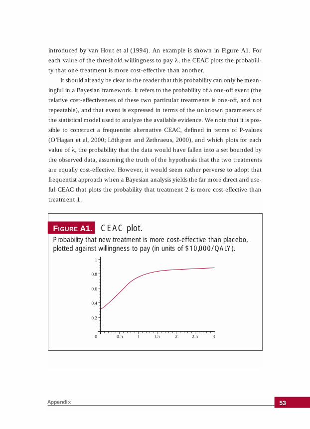
introduced by van Hout et al (1994). An example is shown in Figure A1. For

each value of the threshold willingness to pay λ, the CEAC plots the probabili-

ty that one treatment is more cost-effective than another.

It should already be clear to the reader that this probability can only be mean-

ingful in a Bayesian framework. It refers to the probability of a one-off event (the

relative cost-effectiveness of these two particular treatments is one-off, and not

repeatable), and that event is expressed in terms of the unknown parameters of

the statistical model used to analyze the available evidence. We note that it is pos-

sible to construct a frequentist alternative CEAC, defined in terms of P-values

(O’Hagan et al, 2000; Löthgren and Zethraeus, 2000), and which plots for each

value of λ, the probability that the data would have fallen into a set bounded by

the observed data, assuming the truth of the hypothesis that the two treatments

are equally cost-effective. However, it would seem rather perverse to adopt that

frequentist approach when a Bayesian analysis yields the far more direct and use-

ful CEAC that plots the probability that treatment 2 is more cost-effective than

treatment 1.

Appendix 5353

0.2

0.8

1

0.5 1 1.5 2

0.4

0.6

0 2.5 3

FIGURE A1. CEAC plot. Probability that new treatment is more cost-effective than placebo,plotted against willingness to pay (in units of $10,000/QALY).

The Bayesian Method – Details The following subsections give more details of the Bayesian method.

Bayes’ theorem

The simplest way to express Bayes’ theorem without using mathematical

notation is this:

Several terms in this statement need to be defined and explained. It will be

useful to refer to Figure 1 in the box ‘Example of Bayes’ theorem’. ‘The poste-

rior’ means the posterior distribution of the unknown parameter(s). Strictly, it

is the posterior probability density function, which is shown as the black dotted

curve in Figure 1. Similarly, ‘the prior’ means the prior distribution of the

unknown parameter(s), also in the form of the prior probability density func-

tion and shown as the grey line in Figure 1. The ‘likelihood’ is the common fac-

tor in both frequentist and Bayesian theory. It represents the information in the

data and is shown as the red curve in Figure 1. Formally, for any given value of

the unknown parameter, the likelihood plots the probability of observing the

data that were actually observed. Bayes’ theorem states that we should multi-

ply the two curves. Since the area under any probability density curve must be

equal to one we scale the product to satisfy this condition, which Bayes’

Theorem expresses by saying that the posterior is ‘proportional to’ the product.

Thus, the black dotted curve in Figure 1 results from multiplying the grey and

red curves and scaling the result so that the area under it is equal to one.

This mechanism of multiplying the two curves also makes it clear that

Bayes’ theorem weights each source of information according to its strength.

Consider the situation in which the prior information is very weak. This would

be represented by a very flat grey curve, giving more or less equal prior proba-

bility to a wide range of parameter values. When we apply Bayes’ theorem,

then the posterior becomes almost a constant times the likelihood, and because


The posterior is proportional to the prior times the likelihood.

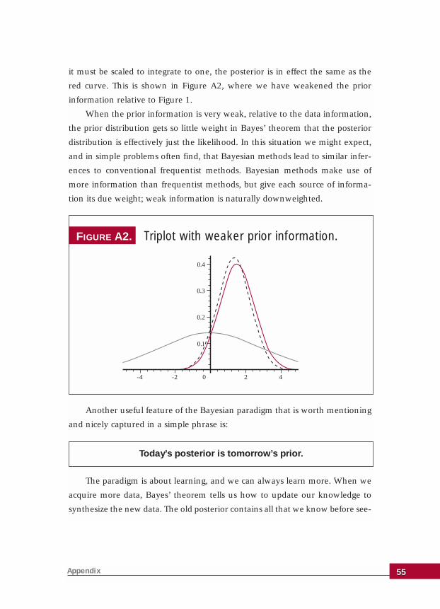
it must be scaled to integrate to one, the posterior is in effect the same as the

red curve. This is shown in Figure A2, where we have weakened the prior

information relative to Figure 1.

When the prior information is very weak, relative to the data information,

the prior distribution gets so little weight in Bayes’ theorem that the posterior

distribution is effectively just the likelihood. In this situation we might expect,

and in simple problems often find, that Bayesian methods lead to similar infer-

ences to conventional frequentist methods. Bayesian methods make use of

more information than frequentist methods, but give each source of informa-

tion its due weight; weak information is naturally downweighted.

Another useful feature of the Bayesian paradigm that is worth mentioning

and nicely captured in a simple phrase is:

The paradigm is about learning, and we can always learn more. When we

acquire more data, Bayes’ theorem tells us how to update our knowledge to

synthesize the new data. The old posterior contains all that we know before see-

Appendix 5555

0.1

0.2

0.3

0.4

-4 -2 0 2 4

FIGURE A2. Triplot with weaker prior information.

Today’s posterior is tomorrow’s prior.

ing the new data, and so becomes the new prior distribution. Bayes’ theorem

synthesizes this with the new data to give the new posterior. And on it

goes…Bayesian methods are ideal for sequential trials!

Bayes’ theorem also makes it more clear as to why the common misinter-

pretation of frequentist inferences is wrong. The likelihood expresses the prob-

ability of obtaining the actual data, given any particular value of the parameter.

In simple terms,

Likelihood = P (data | parameters).

This distribution is the basis of frequentist inference. On the other hand,

the basis of Bayesian inference is the posterior distribution, which is the proba-

bility distribution of the parameters, given the actual data,

Posterior = P (parameters | data).

It is the unjustified switching around of parameters and data that leads to

misinterpretations. For instance, a P-value is P (data | hypothesis), whereas

what a decision-maker wants, and what Bayesian inference provides, is P

(hypothesis | data). It is clear that the two are quite different things, and Bayes’

theorem shows the relationship between them: we can only derive the poste-

rior probability we want by combining the P-value with the prior distribution.

Bayesian inference

In the Bayesian approach, all inferences are derived from the posterior dis-

tribution. When a Bayesian analysis reports a probability interval (a credible

interval) for a parameter, this is a posterior interval, derived from the para-

meter’s posterior distribution, based not only on the data but also on whatever

other information or knowledge the investigator possesses. The probability that

a hypothesis is true is a posterior probability and a typical example of an esti-

mate of a parameter would be the posterior mean (the ‘expected’ value).

These are the Bayesian analogues of the three kinds of inferences that are

available in the frequentist framework. However, Bayesian inference is much

more flexible than this.


Often the real question of interest does not fit one of these frequentist

inference modes. For instance, the investigator frequently wants to know

“What do we now know about this parameter, after seeing the data?” There is

no straightforward frequentist answer to that very natural question. The

Bayesian answer is simplicity itself – we plot the posterior density. Thus, the

black dotted curve in Figure 1 fully expresses what is known about that param-

eter after synthesizing all of the available evidence.

Decision theory provides another good example of the flexibility of

Bayesian inference. In this theory we have a set of possible decisions and a util-

ity function that specifies how good it would be to make a particular decision if

the parameters turned out to have particular values. For instance, for a hypoth-

esis test we could define a utility function that said it would be good (high util-

ity) to accept the hypothesis if it turned out to be true, or to reject it if it turned

out to be false, but otherwise the utility would be low.

If we knew the parameters it would be easy to arrive at a decision – we

would just choose the decision with the largest utility for those values of the

parameters. However, the parameters are generally unknown. Decision theory

says we should choose the decision with the highest (posterior) expected util-

ity. This expectation is the average value of the utility, averaged with respect to

the posterior distribution of the parameters. This is a technical statement, but

the point is that there is no frequentist way to find that optimal decision. It is

essentially a Bayesian construct and is yet another way that the posterior dis-

tribution allows us to answer the real question of interest.

For a health care provider (HCP) choosing between two alternative drugs,

the net benefit is an appropriate utility function. The net benefit (strictly, the

net monetary benefit) of a given drug is obtained by taking the drug’s mean effi-

cacy, multiplying it by the price that the HCP is willing to pay for a unit increase

in efficacy, and then subtracting the mean cost to the HCP of using this drug.

The rule of maximizing expected utility then implies that the HCP should

choose the drug with the larger expected net benefit. Equivalently, it should

choose drug 2 if the expected incremental net benefit over drug 1 is positive

(Claxton, 1999).

Appendix 5757

Prior Information – DetailsThe following subsections give more details of the discussion presented in

the Prior Information section of the main text.

Subjectivity

The fact that Bayesian methods are based on a subjective interpretation of

probability was introduced in the subsection The Nature of Probability in this

Appendix. We explained there that this formulation is necessary if we are to

give probabilities to parameters and hypotheses since the frequentist interpre-

tation of probability is too narrow. Yet this leaves Bayesian methods open to

the charge of subjectivity, which is thought by many to be unacceptable and

unscientific.

Yet science cannot be truly objective. Schools of thought and contention

abound in most disciplines. Science attempts to minimize subjectivity through

the use of objective data and reason, but where the data are not conclusive we

have to use our judgement and expertise.

Bayesian methods naturally accommodate this approach. Figure 1 demon-

strates how Bayes’ theorem naturally weights each information source accord-

ing to its strength. In that example, the data were only slightly more informa-

tive than the prior, and so the posterior is quite strongly influenced by the prior

as well as by the likelihood.

We also saw in Figure A2 how if the prior information is weakened then

Bayes’ theorem effectively places all of the weight on the likelihood. Often we

are in the more fortunate position of having strong data. Then the situation will

be more like the triplot in Figure A3. As new data accumulate the prior distri-

bution again becomes less influential.


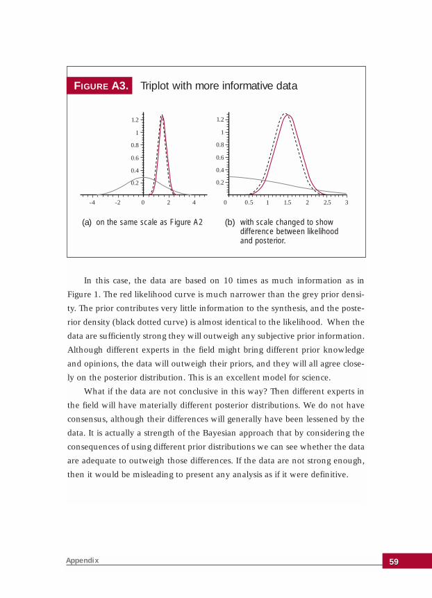
In this case, the data are based on 10 times as much information as in

Figure 1. The red likelihood curve is much narrower than the grey prior densi-

ty. The prior contributes very little information to the synthesis, and the poste-

rior density (black dotted curve) is almost identical to the likelihood. When the

data are sufficiently strong they will outweigh any subjective prior information.

Although different experts in the field might bring different prior knowledge

and opinions, the data will outweigh their priors, and they will all agree close-

ly on the posterior distribution. This is an excellent model for science.

What if the data are not conclusive in this way? Then different experts in

the field will have materially different posterior distributions. We do not have

consensus, although their differences will generally have been lessened by the

data. It is actually a strength of the Bayesian approach that by considering the

consequences of using different prior distributions we can see whether the data

are adequate to outweigh those differences. If the data are not strong enough,

then it would be misleading to present any analysis as if it were definitive.

Appendix 5959

FIGURE A3. Triplot with more informative data

-4 -2 0 2 4

0.2

0.4

0.6

0.8

1.2

1

0.5 1 1.5 2 2.5 30

0.2

0.4

0.6

0.8

1.2

1

(a) (b)on the same scale as Figure A2 with scale changed to show difference between likelihoodand posterior.

Whose prior?

Suppose that a sponsor of some medical technology (e.g. a pharmaceutical

company or device maker) wishes to present a Bayesian analysis in support of

a case for cost-effectiveness of that technology. What would be acceptable in the

form of prior information? One way to approach this question is to ask whose

prior should be used.

As shown above, it may not matter. Consensus can be reached if the data

are strong enough to overrule the differences in the prior opinions and knowl-

edge of all interested parties. However, the argument does not work if one per-

son has sufficiently strong prior information or opinions. It only takes one

extremely opinionated person to prevent agreement. We are familiar with the

person whose views on some matters are so prejudiced that they will not listen

to any facts or arguments to the contrary – Bayes’ theorem explains these peo-

ple, too!

This clarifies some aspects of subjectivity. While we should accept that dif-

ferent people might legitimately have different background knowledge or might

legitimately interpret the same information differently, there is no place for

prejudice or perverse misinterpretation of the available facts in health econom-

ics (or anywhere else). An important aspect of Bayesian analysis is that the prior

distribution is set out openly. If it is not based on reasonable use of information

and experience, the resulting analysis will not convince anyone. This is the key

benefit (B5) – “more open judgements” – of Bayesian analysis. All cards should

be on the table and nothing hidden.

Returning to the question of whose prior a sponsor might use, it is likely

that the sponsor’s own prior distribution would be unacceptable. In principle,

their opinions might be defensible on the basis of the company’s own substan-

tial experiences in development and testing of the product, but there is the risk

of selective use of information unless full disclosure can be enforced. To quote

the box “The Evidence” in the main text, the sponsor would need to be able to

show that its prior not only represented the evidence but also the whole evi-

dence.

The most natural choice of prior distribution might be the considered and

defensible prior of an expert in the field. The agency to which the cost-effec-


Appendix 6161

tiveness case is being made would probably be interested in whether the infer-

ences might change if the views of alternative experts were considered. Ideally,

some kind of consensus view of the profession would be a good choice.

Examples

These ideas are illustrated in the following two examples, which are dis-

cussed briefly in the main text.

Subset analysis is a notoriously tricky question. The risk of dredging the

data to find subgroups of patients that respond differently is real. For example,

suppose that a cost study found the following mean costs table (Table 2), split

by treatment and the initial letter of the patient’s surname.

It looks like treatment 2 is cheaper for patients whose names begin with the

letters A to D. There is highly unlikely to be any plausible reason for such a sub-

group effect. To avoid the risk of declaring spurious subgroup effects, standard

clinical trials guidance requires that the analysis of possible subgroups must be

specified before a trial begins, and there must be a plausible mechanism for the

proposed subgroup effects.

From a Bayesian perspective, the absence of a plausible mechanism simply

constitutes prior information – the subgroup effect would have a very small

prior probability. Combining the prior information with the data would result

in a small posterior probability, regardless of how convincing the data appeared

to be. The prior information is strong enough to override the data. The standard

guidance, therefore, applies equally to Bayesian analyses; subgroup analyses

must be prespecified, so that prior information about their plausibility can be

quantified.

Treatment 1

Treatment 2

NAMES A-D NAMES E-Z

$800

$450

$800

$850

TABLE 2. Mean costs in hypothetical trial

Bayesian methods will then automatically moderate the data and prevent

us from claiming implausible effects that arise by chance in the data. The prior

information is clearly important. To an extent, the existing procedures for fre-

quentist subgroup analysis incorporate the prior information (and so, we would

argue, are unconsciously Bayesian). However, the frequentist analysis simply

splits subgroup hypotheses into those that are plausible a priori and those that

are not, whereas the Bayesian assigns a prior probability that can take any value

from 0 to 1, and thereby allows a far more subtle gradation.

Hospitalization. Suppose that, after evaluating good evidence on efficacy of

a new drug relative to the standard treatment, a decision on whether it is more

cost-effective rests on whether it reduces hospitalizations. Here the data come

from a trial in which the number of days in hospital was recorded for each of

100 patients in each treatment group. A total of 25 hospital days were record-

ed in the standard treatment group and only 5 in the group receiving the new

drug. In frequentist terms, the difference is found to be significant at the 5%

level (one-sided). (We will not give technical details of calculations, but all of

this, and subsequent analysis, may be reconstructed using the additional infor-

mation that the sample variances were 1.2 in the standard treatment group and

0.248 in the new drug group.) The drug company could then, in conventional

frequentist terms, claim an effect on hospitalization, estimate the mean number

of days per patient as 0.25 under standard treatment and 0.05 under the new

drug, perhaps with the result that the new drug is now found to be more cost-

effective than standard treatment.

This is, however, a rather small trial and the data are far from conclusive.

If other evidence were available it would be prudent to incorporate it in the

analysis. Suppose that a much larger trial (in comparable conditions) of a simi-

lar drug produced a mean number of days in hospital per patient of 0.21, and

that the standard error of this estimate is only about 0.03. This extra informa-

tion suggests that the observed rate of 0.05 for the new drug is optimistic and

casts doubt on the magnitude of the real difference between it and standard

treatment. However, the interpretation of this evidence is necessarily judgmen-

tal. Nobody would claim that the two drugs should necessarily yield the same


hospitalization rates, but it is reasonable to suppose that they would not be

markedly different. Because they cannot be treated as completely comparable

with the trial data on the new drug, we cannot treat this other, larger trial as

part of the data and just merge it with the new data. There is no apparent way

to use the evidence on the related drug in a frequentist analysis. Yet any clini-

cian or health care provider who was aware of this external evidence would be

disinclined to take the new trial evidence at face value.

A Bayesian analysis resolves the question by treating the earlier trial as pro-

viding prior information but entails an element of subjectivity. Suppose that

your interpretation of the prior information is that your prior expectation of the

mean days in hospital for the new drug should be 0.21 but with a standard devi-

ation of 0.08 to reflect the fact that the two drugs are not the same. Bayes’ the-

orem now yields for you a posterior estimate of 0.095 for the mean hospital

days using the new drug. There is still a reasonably strong probability (90%)

that the new drug reduces this hospitalization rate, but now the estimated dif-

ference may not be large enough to provide the same assurance that it is more

cost-effective than standard treatment.

The subjectivity in this analysis arises in the necessary judgement about

how different the hospitalization rates might be for the two drugs. Another cli-

nician or decision-maker might interpret the prior information differently and

employ a different prior distribution. In particular, they may have a different

prior standard deviation. In fact this answer is fairly robust to reasonable

changes in the prior distribution. On that basis we might conclude that an

‘objective’ interpretation of the combined data is that there is a strong proba-

bility (perhaps around 90% but not as high as 95%) that the new drug reduces

mean days in hospital but that it achieves a mean number of days nearer to 0.1

than to 0.05.

This example has shown how a Bayesian analysis, making use of genuine

prior information and considering a range of reasonable interpretations of that

information, can produce a scientifically sound conclusion. The answer differs

substantially from the frequentist analysis which has no technical way of mak-

ing use of the extra information. The Bayesian answer is also sound because it

formalizes the natural intuitive reaction that anyone would have to the fre-

Appendix 6363

quentist analysis, knowing the result of the other trial.

In this and previous examples, we have stressed the power of the Bayesian

approach to temper overly optimistic interpretations of P-values, but it is impor-

tant to recognize that the reverse situation is equally common and important.

Pharmaceutical company executives and biostatisticians will be very familiar

with occasions where a Phase III trial of a drug has just failed to produce a sig-

nificant effect, yet there is plenty of evidence (from related drugs, from a Phase

II trial that was restricted to acute cases, etc.) to suggest that the drug really is

effective. A properly conducted Bayesian analysis would allow the responsible

incorporation of this additional evidence to demonstrate the drug’s true efficacy.

Both situations are of enormous importance to the developers and users of

health care technologies –the first in avoiding costly mistakes due to being over-

ly optimistic and the second in allowing beneficial products to be brought to mar-

ket that otherwise would have to be abandoned or delayed for more testing.

Prior Specification – DetailsThe following subsections give details of three aspects of prior specification;

the elicitation of expert priors, conjugate priors and the construction of struc-

tural priors.

Elicitation

We will consider the process of eliciting a prior distribution for an expert

without reference to the actual nature of the underlying prior information. In

practice, of course, the expert will base her analysis on that information, but in

this subsection we will not try to deal with the specifics of the underlying

information.

Suppose that we decide to formulate a prior distribution for a particular

parameter (such as the mean utility gain arising from some treatment), repre-

senting the knowledge of a single expert about that parameter. The first diffi-

culty we will face is that the expert will almost certainly not be an expert in

probability or statistics. That means it will not be easy for this person to express

her beliefs in the kind of probabilistic form demanded by Bayes’ theorem.

Our expert might be willing to give us an estimate of the parameter, but


how do we interpret this? Should we treat it as the mean (or expectation) of the

prior distribution, or as the median of that distribution, as its mode, or something

else? In statistics, the mean, median and mode might all be regarded as sound

point estimates of a quantity, but they are different things. The mean is the

‘expected value’, the median is the ‘central value’ and the mode is the ‘most like-

ly value’. In principle, we might explore with the expert these nuances of mean-

ing, but for someone not trained in statistics it will not be easy for her to appre-

ciate the differences and give us a reliable interpretation for her estimate.

We could go on to elicit from the expert some more features of her distri-

bution, such as some measure of spread to indicate her general level of uncer-

tainty about the true value of the parameter. (Remember, the strength of infor-

mation is indicated by the narrowness of the distribution representing that

information.)

The next difficulty is that no matter how much information of this type we

extract from the expert it will not be enough to identify her distribution exact-

ly. This is easy to see when we recognize that to uniquely identify the grey curve

in Figure 1 representing the prior distribution, we must specify its height at

every single point – potentially an infinite number of facts must be obtained

from the expert. To compound this problem, the more detail we ask for, the

more difficult it is for the expert. In practice, the best we can do is to elicit a few

simple expressions of her knowledge, in the form of things like median and

quartiles and then fit some sensible distribution to those statements.

Even the judgements that we elicit from the expert cannot be treated as

precise. Suppose that the expert gives us the estimate of 0.85 for the parame-

ter, and we interpret this as the mean of her prior distribution. Even if we are

right to interpret it in that way, we cannot realistically treat it as a precise num-

ber. Our expert almost certainly gave us a round figure and couldn’t say

whether 0.86 might be a more accurate reflection of her prior mean. The read-

er should now amply appreciate the criticism (D2), that “prior specification is

unreliable”.

Nevertheless, there is a growing body of research into how to elicit experts’

knowledge accurately and reliably. The difficulties that people face in assessing

probabilities have been extensively studied, particularly by cognitive psycholo-

Appendix 6565

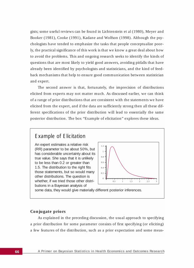
gists; some useful reviews can be found in Lichtenstein et al (1980), Meyer and

Booker (1981), Cooke (1991), Kadane and Wolfson (1998). Although the psy-

chologists have tended to emphasize the tasks that people conceptualize poor-

ly, the practical significance of this work is that we know a great deal about how

to avoid the problems. This and ongoing research seeks to identify the kinds of

questions that are most likely to yield good answers, avoiding pitfalls that have

already been identified by psychologists and statisticians, and the kind of feed-

back mechanisms that help to ensure good communication between statistician

and expert.

The second answer is that, fortunately, the imprecision of distributions

elicited from experts may not matter much. As discussed earlier, we can think

of a range of prior distributions that are consistent with the statements we have

elicited from the expert, and if the data are sufficiently strong then all these dif-

ferent specifications of the prior distribution will lead to essentially the same

posterior distribution. The box “Example of elicitation” explores these ideas.

Conjugate priors

As explained in the preceding discussion, the usual approach to specifying

a prior distribution for some parameter consists of first specifying (or eliciting)

a few features of the distribution, such as a prior expectation and some meas-


Example of ElicitationAn expert estimates a relative risk(RR) parameter to be about 50%, buthas considerable uncertainty about itstrue value. She says that it is unlikelyto be less than 0.2 or greater than1.5. The distribution to the right fitsthose statements, but so would manyother distributions. The question iswhether, if we tried those other distri-butions in a Bayesian analysis ofsome data, they would give materially different posterior inferences.

0

0.2

0.4

0.6

0.8

1

1.2

0.5 1 1.5 2 2.5 3

ure of prior uncertainty (e.g. the prior variance), then choosing a suitable dis-

tribution to fit these features. In the box “Example of elicitation”, for instance,

a particular form of distribution known as a gamma distribution has been fitted

to the expert’s two specific statements.

This may seem rather cavalier and arbitrary, but in practice the prior distri-

bution is often quite well determined even if only a few actual features have

been specified or elicited from the expert. Although the actual distribution cho-

sen is arbitrary, any other reasonable prior distribution that fits the specifica-

tions is likely to be very similar, and hence to lead to very similar inferences or

decisions.

It is then sensible to make the choice of distributions on grounds of sim-

plicity and convenience. Mathematically, in some simple statistical problems

there exist classes of priors known as conjugate priors that are particularly con-

venient. This is because of two features. First, if the prior distribution is a mem-

ber of the relevant conjugate class then the posterior distribution will also be a

member of that class. Second, the conjugate distributions are sufficiently simple

for us to be able to derive a great many inferences from them without resort to

computational methods. Whenever the statistical model is such that a conjugate

family exists and a member of that family fits the prior specification, then it is

particularly convenient to choose that distribution. Very simple posterior analy-

sis then follows.

Indeed, in the early days of modern Bayesian statistics, in the 1960s and

1970s, Bayesian analysis was essentially restricted to the use of conjugate pri-

ors, since computational tools did not exist to tackle more complex situations.

They are now much less used because statisticians are building models that do

not have corresponding conjugate priors, and the desire for more realistic for-

mulation of prior information also means that conjugate priors may not fit even

when they are available.

Structural priors

Structural prior distributions express information about relationships

between parameters, usually without saying anything about the specific values

of individual parameters. For instance, we might specify a prior distribution that

Appendix 6767

represents effective ignorance about the mean cost under two different treat-

ments, but says that we expect the ratio of these means to be in the range 0.2

to 5. The mean cost under any given treatment could be anything at all, but

whatever value it actually takes we expect the mean cost under the other treat-

ment will be within a factor of 5 of this.

A simple example is the prior distribution in the example of hospitaliza-

tion. This can be dissected into two parts. We have substantial prior informa-

tion about mean days in hospital under the related drug, and we have struc-

tural prior information about how it might differ from the corresponding mean

hospitalization under the new drug. Indeed, if the raw data of the earlier trial

are available we might formally analyze these as data with the results of the

new trial. In that case, the prior information is purely structural. The frame-

work now looks a little like a meta-analysis, and indeed Bayesian meta-analy-

sis is based strongly on structural prior information.

In a Bayesian meta-analysis, we have several datasets, each of which

addresses the efficacy of a treatment in slightly different conditions. So we

have a separate parameter for mean efficacy in each trial, but we formulate a

structural prior representing the prior expectation that these parameters

should not be too different. This is usually done in a hierarchical model,

where a common ‘underlying’ mean efficacy parameter is postulated, and each

of the trial mean efficacies is considered to be independently distributed

around this common parameter.

The hierarchical structure, introducing one or more common parameters,

is often used to link several related parameters and to express a belief that they

should be similar via the fact that they should all be similar to the common

parameter. Another example is to formulate structural prior information that

cost data arising in different arms of a trial should not be markedly different in

their degrees of skewness. This has the benefit of moderating the influence of

a very small number of patients with unusually high costs.

Computation – DetailsThe following subsections give details of Bayesian computation and its

ability to address very complex models.


Complexity

The source of the extra complexity in Bayesian analysis is again the prior

distribution. Suppose that the problem is the simple, canonical, statistical prob-

lem of estimating the mean of a normal distribution (with known variance),

given a sample from that distribution. To the frequentist, this is a complete spec-

ification of the problem, and in principle there can be a single answer (and in

fact the sample mean is universally accepted as the best estimate). To the

Bayesian, the specification is incomplete because we also need to state the prior

distribution. Then the answer will synthesize the two information sources and

will depend on the prior. Given this simple problem, the Bayesian approach can

give a very wide range of answers.

This makes the construction of Bayesian software very difficult. The software

itself must be more complex. The reason for this is because it must allow for spec-

ification of the prior (which could be any distribution at all) and must be able to

compute the desired inferences no matter what that prior distribution may be.

Mathematically, Bayesian inferences usually require us to be able to inte-

grate the product of the prior and the likelihood. We have to do this, for

instance, just to find the area under the curve, so as to know how to scale it to

make that area 1. Just applying Bayes’ theorem demands integration. More

integration is then needed, for instance, to find the posterior mean or the prob-

ability that a hypothesis is true. Now even if the prior and the likelihood are

individually quite nice functions whose integrals are well known, the product

will almost invariably be sufficiently complex for us to be unable to derive the

necessary integrals by mathematical principles. So these integrals need to be

done numerically (for an introduction to the ideas and methods of numerical

integration, see Thisted, 1988). The main reason why Bayesian methods were

impractical until the 1990s was that we did not have effective integration algo-

rithms. The reason for the subsequent explosion of Bayesian applications is that

a very powerful, general solution was developed.

MCMC

The technique that has revolutionized Bayesian computation is Markov

chain Monte Carlo (MCMC). The idea of MCMC has been outlined in the main

Appendix 6969

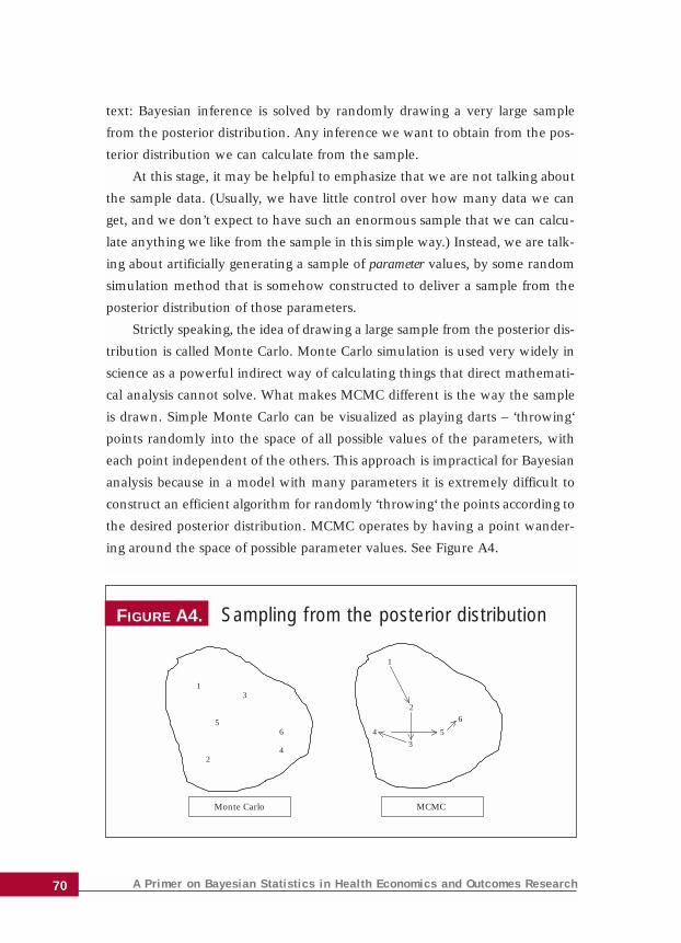
text: Bayesian inference is solved by randomly drawing a very large sample

from the posterior distribution. Any inference we want to obtain from the pos-

terior distribution we can calculate from the sample.

At this stage, it may be helpful to emphasize that we are not talking about

the sample data. (Usually, we have little control over how many data we can

get, and we don’t expect to have such an enormous sample that we can calcu-

late anything we like from the sample in this simple way.) Instead, we are talk-

ing about artificially generating a sample of parameter values, by some random

simulation method that is somehow constructed to deliver a sample from the

posterior distribution of those parameters.

Strictly speaking, the idea of drawing a large sample from the posterior dis-

tribution is called Monte Carlo. Monte Carlo simulation is used very widely in

science as a powerful indirect way of calculating things that direct mathemati-

cal analysis cannot solve. What makes MCMC different is the way the sample

is drawn. Simple Monte Carlo can be visualized as playing darts – ‘throwing‘

points randomly into the space of all possible values of the parameters, with

each point independent of the others. This approach is impractical for Bayesian

analysis because in a model with many parameters it is extremely difficult to

construct an efficient algorithm for randomly ‘throwing‘ the points according to

the desired posterior distribution. MCMC operates by having a point wander-

ing around the space of possible parameter values. See Figure A4.


FIGURE A4. Sampling from the posterior distribution

13

2

56

4

1

4

3

2

5

6

Monte Carlo MCMC

Technically, a probability model called a Markov chain generates this wan-

dering point. Successive steps in this Markov chain produce the sample. It turns

out that it is really quite simple to construct a Markov chain such that the sam-

ple is drawn from any desired posterior distribution.

The power of Bayesian computations derives from the availability of

MCMC solutions to compute posterior inferences from almost arbitrarily

complex statistical models with almost arbitrarily huge numbers of parame-

ters. However, this simple statement hides some important complications.

It is clear that these successive values are connected and not independent

in the way that simple Monte Carlo points are. If there is too much depend-

ence, then the points move very slowly around the space of possible param-

eter values. Therefore, an extremely large sample will be needed to cover the

space properly to represent the posterior distribution adequately. So the effi-

ciency of MCMC methods depend critically on getting a Markov chain that

moves rapidly around the space (a property that is referred to as ‘good mix-

ing’). Unfortunately, although it is generally very easy to devise an MCMC

algorithm that works in principle, it often requires considerable skill and

experience to construct one that mixes well.

Another complication is that the algorithms require a ‘burn-in’ period,

for the randomly moving point to settle into the part of the parameter space

supported by the posterior distribution. It is by no means simple to diagnose

when the Markov chain has run long enough.

In a very wide range of moderately complex models (such as those that

can be implemented successfully in the software WinBUGS described in the

main text), these problems are minimal. For large and complex problems,

however, MCMC remains something of an arcane art. Nevertheless, there is

growing familiarity with the technique based on its widespread use in

Bayesian statistics – and a growing literature on MCMC algorithms that is

gradually advancing the frontier of problems that can be tackled routinely.

Appendix 7171

Tackling hard problems

There is a frequentist parallel to the computational problems of Bayesian

methods, which is that it is extremely difficult to obtain exact frequentist tests,

confidence intervals and unbiased estimators except in really simple models. It

is often overlooked that the great majority of frequentist techniques in general

use are, in fact, only approximate. This includes all methods based on general-

ized linear models, generalized likelihood ratio tests, bootstrapping and many

more. The honorable exception is inference in the standard normal linear

model. Even here, it is not straightforward to compare non-nested models using

frequentist methods.

As described in the main text, the availability of computational techniques

like MCMC makes exact Bayesian inferences possible even in very complex

models. As statisticians strive to address larger, more complex data structures

(micro-array data, data mining, etc), the benefit (B3) – “ability to tackle more

complex problems” – of Bayesian methods becomes increasingly important.


Documents

Primer on Bayesian statistics - University of Sheffield