To be published in The Journal of the Royal Society Interface (2014)

Mapping the stereotyped behaviour of freely-moving fruit flies

Gordon J. Berman,1 Daniel M. Choi,2 William Bialek,1 and Joshua W. Shaevitz1, ∗

1Joseph Henry Laboratories of Physics and Lewis-Sigler Institute for Integrative Genomics2Department of Molecular Biology

Princeton UniversityPrinceton, NJ 08544

(Dated: November 11, 2018)

A frequent assumption in behavioural science is that most of an animal’s activities can be describedin terms of a small set of stereotyped motifs. Here we introduce a method for mapping an animal’sactions, relying only upon the underlying structure of postural movement data to organise andclassify behaviours. Applying this method to the ground-based behaviour of the fruit fly, Drosophilamelanogaster, we find that flies perform stereotyped actions roughly 50% of the time, discovering over100 distinguishable, stereotyped behavioural states. These include multiple modes of locomotionand grooming. We use the resulting measurements as the basis for identifying subtle sex-specificbehavioural differences and revealing the low-dimensional nature of animal motions.

I. INTRODUCTION

The concept of stereotypy–that an organism’s be-haviours can be decomposed into discrete, reproducibleelements–has influenced the study of ethology, be-havioural genetics, and neuroscience for decades [1, 2].Animals possess the ability to move in a vast continuumof ways, theoretically constrained only by the biome-chanical limits of their own morphology. Despite this,the range of behavioural actions typically performed byan animal is thought to be much smaller, constructedlargely of stereotyped actions that are consistent acrosstime, individuals, and, in some cases, even species [3, 4].A discrete behavioural repertoire can potentially arisevia a number of mechanisms, including mechanical limitsof gait control, habit formation, and selective pressure togenerate robust or optimal actions. In many instances,the search for an individual behavioural neural circuitor gene begins with the assumption that a particular ac-tion of interest is stereotyped across time and individuals[5, 6].

Despite the centrality of this concept, with few ex-ceptions [7–11], the existence of stereotypy has not beenprobed experimentally. This is largely due to the lackof a comprehensive and compelling mathematical frame-work for behavioural analysis. Here, we introduce a newmethod for quantifying postural dynamics that retainsan animal’s full behavioural complexity, using the fruitfly Drosophila melanogaster as a model organism to dis-cover and map stereotyped motions.

Most prior methods for quantifying animal behaviourlie in one of two regimes. One of these is the use of coarsemetrics such as a gross activity level (e.g. mean veloc-ity or number of times the organism crosses a barrier)or counting the relative frequencies of particular eventsengrained into the experimental set-up (e.g. turning leftor right in a maze). While this approach allows for high-throughput analysis of various organisms, strains, and

∗ Corresponding author: shaevitz@princeton.edu

species, only the most gross aspects of behaviour canbe ascertained, potentially overlooking the often sub-tle effects of the manipulations of interest that are onlyapparent at a finer descriptive level. The other com-mon approach for behavioural quantification is to use aset of user-defined behavioural categories. These cate-gories, such as walking, grooming, or fighting, are codi-fied heuristically and scored either by hand or, more re-cently, via supervised machine-learning techniques [12–16]. While the latter approach allows for higher through-put and more consistent labeling, it remains prone tohuman bias and anthropomorphism and often precludesobjective comparisons between data sets due to the re-liance on subjective definitions of behaviour. Further-more, these analyses assume, a priori, that stereotypedclasses of behaviour exist without first showing, fromthe data, that an organism’s actions can be meaning-fully categorised in a discrete manner.

Ideally, a behavioural description should manifest it-self directly from the data, based upon clearly-statedassumptions, each with testable consequences. The ba-sis of our approach is to view behaviour as a trajec-tory through a high-dimensional space of postural dy-namics. In this space, discrete behaviours correspondto epochs in which the trajectory exhibits pauses, cor-responding to a temporally-extended bout of a particu-lar set of motions. Epochs that pause near particular,repeatable positions represent stereotyped behaviours.Moreover, moments in time in which the trajectory isnot stationary, but instead moves rapidly, correspond tonon-stereotyped actions.

In this paper, we construct a behavioural space forfreely-moving fruit flies. We observe that the flies ex-hibit approximately 100 stereotyped behaviours that areinterspersed with frequent bouts of non-stereotyped be-haviours. These stereotyped behaviours manifest them-selves as distinguishable peaks in the behavioural spaceand correspond to recognizably distinct behaviours suchas walking, running, head grooming, wing grooming, etc.Using this framework, we begin to address biologicalquestions about the underlying postural dynamics thatgenerate behaviour, opening the door for a wide range

arX

iv:1

310.

4249

v2 [

q-bi

o.Q

M]

12

Aug

201

4

2

FIG. 1. Schematic of the imaging apparatus.

of other inquiries into the dynamics, neurobiology, andevolution of behaviour.

II. EXPERIMENTS

We probed the spontaneous behaviours of ground-based flies (Drosophila melanogaster) in a largely fea-tureless circular arena (Fig 1). Under these condi-tions, flies display a multitude of complex, non-aerialbehaviours such as locomotion and grooming, typicallyinvolving multiple parts of their bodies. To capture dy-namic rearrangements of the fly’s posture, we recordedvideo of individual behaving animals with sufficient spa-tiotemporal resolution to resolve moving body parts suchas the legs, wings, and proboscis.

We designed our arena based on previous work whichshowed that a thin chamber with gently sloping sides pre-vents flies from flying, jumping, and climbing the walls[17]. To keep the flies in the focal plane of our camera,we inverted the previous design. Our arena consists of acustom-made vacuum-formed, clear PETG plastic dome100mm in diameter and 2mm in height with sloping sidesat the edge clamped to a flat glass plate. The edges of theplastic cover are sloped to prevent the flies from beingoccluded and to limit their ability to climb upside-downon the cover. The underside of the dome is coated witha repellent silane compound (heptane and 1,7-dichloro-1,1,3,3,5,5,7,7-octamethylte-trasiloxane) to prevent theflies from adhering to the surface. In practice, we findthat this set-up results in no bouts of upside-down walk-ing.

Over the course of these experiments, we studied thebehaviour of 59 male and 51 female D. melanogaster(Oregon-R strain). Each animal was imaged usinga high-speed camera (100 Hz, 1088 × 1088 pixels).A proportional-integral-derivative (PID) feedback algo-rithm is used to keep the moving fly inside the cameraframe by controlling the position of the X-Y stage based

on the camera image in real time. In each frame wefocus our analysis on a 200 × 200 pixel square contain-ing the fly. We imaged each of the flies for one hour,yielding 3.6 × 105 movie frames per individual, or ap-proximately 4 × 107 frames in total. All aspects of theinstrumentation are controlled by a single computer us-ing a custom-written LabView graphical user interface.

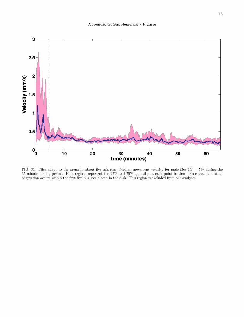
Each of these flies was isolated within 4 hours of eclo-sion and imaging occurred 1-14 days after that. Flieswere placed into the arena via aspiration and were sub-sequently allowed 5 minutes for adaptation before datacollection (Fig S1). All recording occurred between thehours of 9:00 AM and 1:00 PM, thus reducing the ef-fect of circadian rhythms, and the temperature duringall recordings was 25o ± 1oC.

III. BEHAVIOURAL ANALYSIS

The general framework of our analysis is describedin Fig 2. Images are first segmented and registered inorder to isolate the fly from the background and en-force translational and rotational invariance. After this,they are decomposed into postural time series and con-verted into wavelet spectrograms, thus creating a spatio-temporal representation for the fly’s dynamics within theimages. These spectrograms are used to construct spec-tral feature vectors that we embed into two dimensionsusing t-Distributed Stochastic Neighbor Embedding [18].Lastly, we estimate the probability distribution over thistwo dimensional space and identify resolvable peaks inthe distribution. We confirm that sustained pauses nearthese peaks correspond to discrete behavioural states.

A. Image segmentation and registration

Given a sequence of images, we wish to build a spatio-temporal representation for the fly’s postural dynamics.We start by isolating the fly within each frame, followedby rotational and translational registration to produce asequence of images in the coordinate frame of the insect.Details of these procedures are listed in Appendix A. Inbrief, we apply Canny’s method for edge detection [19],morphological dilation, and erosion to create a binarymask for the fly. After applying this mask, we rotation-ally align the images via polar cross-correlation with atemplate image, similar to previously developed methods[20–22]. We then we use a sub-pixel cross-correlation totranslationally align the images [23]. Lastly, every imageis re-sized so that, on average, each fly’s body covers thesame number of pixels. An example segmentation andalignment is shown in Supplementary Movie S1.

B. Postural decomposition

As the fly body is made up of relatively inflexible seg-ments connected by mobile joints, the number of postu-

3

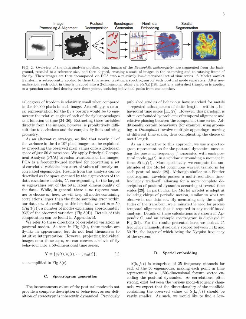
FIG. 2. Overview of the data analysis pipeline. Raw images of the Drosophila melanogaster are segmented from the back-ground, rescaled to a reference size, and then aligned, creating a stack of images in the co-moving and co-rotating frame ofthe fly. These images are then decomposed via PCA into a relatively low-dimensional set of time series. A Morlet wavelettransform is subsequently applied to these time series, creating a spectrogram for each postural mode separately. After nor-malization, each point in time is mapped into a 2-dimensional plane via t-SNE [18]. Lastly, a watershed transform is appliedto a gaussian-smoothed density over these points, isolating individual peaks from one another.

ral degrees of freedom is relatively small when comparedto the 40,000 pixels in each image. Accordingly, a natu-ral representation for the fly’s posture would be to enu-merate the relative angles of each of the fly’s appendagesas a function of time [24–26]. Extracting these variablesdirectly from the images, however, is prohibitively diffi-cult due to occlusions and the complex fly limb and winggeometry.

As an alternative strategy, we find that nearly all ofthe variance in the 4×104 pixel images can be explainedby projecting the observed pixel values onto a Euclideanspace of just 50 dimensions. We apply Principal Compo-nent Analysis (PCA) to radon transforms of the images.PCA is a frequently-used method for converting a setof correlated variables into a set of values of linearly un-correlated eigenmodes. Results from this analysis can bedescribed as the space spanned by the eigenvectors of thedata covariance matrix, C, corresponding to the largestm eigenvalues out of the total latent dimensionality ofthe data. While, in general, there is no rigorous man-ner to choose m, here, we will keep all modes containingcorrelations larger than the finite sampling error withinour data set. According to this heuristic, we set m = 50(Fig 3(c)), a number of modes explaining approximately93% of the observed variation (Fig 3(d)). Details of thiscomputation can be found in Appendix B.

We refer to these directions of correlated variation aspostural modes. As seen in Fig 3(b), these modes arefly-like in appearance, but do not lend themselves tointuitive interpretation. However, projecting individualimages onto these axes, we can convert a movie of flybehaviour into a 50-dimensional time series,

Y ≡ {y1(t), y2(t), · · · , y50(t)}, (1)

as exemplified in Fig 3(e).

C. Spectrogram generation

The instantaneous values of the postural modes do notprovide a complete description of behaviour, as our defi-nition of stereotypy is inherently dynamical. Previously

published studies of behaviour have searched for motifs– repeated subsequences of finite length – within a be-havioural time series [11, 27]. However, this paradigm isoften confounded by problems of temporal alignment andrelative phasing between the component time series. Ad-ditionally, certain behaviours (for example, wing groom-ing in Drosophila) involve multiple appendages movingat different time scales, thus complicating the choice ofmotif length.

As an alternative to this approach, we use a spectro-gram representation for the postural dynamics, measur-ing the power at frequency f associated with each pos-tural mode, yk(t), in a window surrounding a moment intime, S(k, f ; t). More specifically, we compute the am-plitudes of the Morlet continuous wavelet transform foreach postural mode [28]. Although similar to a Fourierspectrogram, wavelets possess a multi-resolution time-frequency trade-off, allowing for a more complete de-scription of postural dynamics occurring at several timescales [29]. In particular, the Morlet wavelet is adept atisolating chirps of periodic motion, similar to what weobserve in our data set. By measuring only the ampli-tudes of the transform, we eliminate the need for precisetemporal alignment that is required in any motif-basedanalysis. Details of these calculations are shown in Ap-pendix C, and an example spectrogram is displayed inFig 3(f). For the results presented here, we look at 25frequency channels, dyadically spaced between 1 Hz and50 Hz, the larger of which being the Nyquist frequencyof the system.

D. Spatial embedding

S(k, f ; t) is comprised of 25 frequency channels foreach of the 50 eigenmodes, making each point in timerepresented by a 1,250-dimensional feature vector en-coding the postural dynamics. As correlations, oftenstrong, exist between the various mode-frequency chan-nels, we expect that the dimensionality of the manifoldcontaining the observed values of S(k, f ; t) should bevastly smaller. As such, we would like to find a low-

4

FIG. 3. Generation of spectral feature vectors. (a) Raw image of a fly in the arena. (b) Pictorial representation of the first5 postural modes, x1−5, after inverse Radon transform. Black and white regions represent highlighted areas of each mode(with opposite sign). (c) First 1,000 eigenvalues of the data matrix (black) and shuffled data (red). (d) Fraction of cumulativevariation explained as a function of number of modes included. (e) Typical time series of the projection along postural mode6 and (f) its corresponding wavelet transform.

dimensional representation that captures the importantfeatures of the data set.

Our strategy for dimensional reduction of the featurevectors is to construct a space, B, such that trajecto-ries within it pause near a repeatable position whenevera particular stereotyped behaviour is observed. Thismeans that our embedding should minimise any localdistortions. However, we do not require preservation ofstructure on longer length scales. Hence, we chose anembedding that reduces dimensionality by altering thedistances between more distant points on the manifold.

Most common dimensionality reduction methods, in-cluding PCA, Multi-dimensional scaling, and Isomap,do precisely the opposite, sacrificing local verisimilitudein service of larger-scale accuracy [30–32]. One methodthat does possess this property is t-Distributed Stochas-tic Neighbor Embedding (t-SNE) [18]. Like other em-bedding algorithms, t-SNE aims to take data from ahigh-dimensional space and embed it into a space ofmuch smaller dimensionality, preserving some set of in-variants as best as possible. For t-SNE, the conservedinvariants are related to the Markov transition proba-bilities if a random walk is performed on the data set.Specifically, we define the transition probability fromtime point ti to time point tj , pj|i, to be proportionalto a Gaussian kernel of the distance (as of yet, unde-fined) between them:

pj|i =exp(− d(ti, tj)

2/2σ2i

)∑k 6=i exp

(− d(ti, tk)2/2σ2

i

) . (2)

All self-transitions (i.e. pi|i) are assumed to be zero.Each of the σi are set such that all points have the sametransition entropy, Hi =

∑j pj|i log pj|i = 5. This can

be interpreted as restricting transitions to roughly 32neighbors.

The t-SNE algorithm then embeds the data points inthe smaller space while keeping the new set of transitionprobabilities, qj|i, as similar to the pj|i as possible. Theqj|i are defined similarly to the larger-space transitionprobabilities, but are now, for technical reasons, propor-tional to a Cauchy (or Student-t) kernel of the points’Euclidean distances in the embedded space. This algo-rithm results in an embedding that minimises local dis-tortions [18]. If pj|i is initially very small or zero, it willplace little to no constraint on the relative positions ofthe two points, but if the original transition probabilityis large, it will factor significantly into the cost function.

This method’s primary drawback, however, is its poormemory complexity scaling (∝ N2). To incorporate ourentire data set into the embedding, we use an importancesampling technique to select a training set of 35,000 datapoints, build the space from these data, and then re-embed the remaining points into the space as best aspossible (see Appendix D for implementation details).

Lastly, we need to define a distance function, d(ti, tj),between the feature vectors. We desire this functionto accurately measure how different the shapes of twomode-frequency spectra are, ignoring the overall mul-tiplicative scaling that occurs at the beginning andthe end of behavioural bouts due to the finite natureof the wavelet transform. Simply measuring the Eu-

5

clidean norm between two spectra will be greatly af-fected by such amplitude modulations. However, be-cause S(k, f ; t) is composed of a set of wavelet ampli-tudes, it must therefore be positive semi-definite. Assuch, if we define

S(k, f ; t) ≡ S(k, f ; t)∑k′,f ′ S(k′, f ′; t)

, (3)

then we can treat this normalised feature vector as aprobability distribution over all mode-frequency chan-nels at a given point in time. Hence, a reasonable dis-tance function is the Kullback-Leibler (KL) divergence[33] between two feature vectors:

d(t1, t2) = DKL(t1||t2)

≡∑f,k

S(k, f ; t1) log2

[S(k, f ; t1)

S(k, f ; t2)

]. (4)

IV. RESULTS

A. Embedded space dynamics

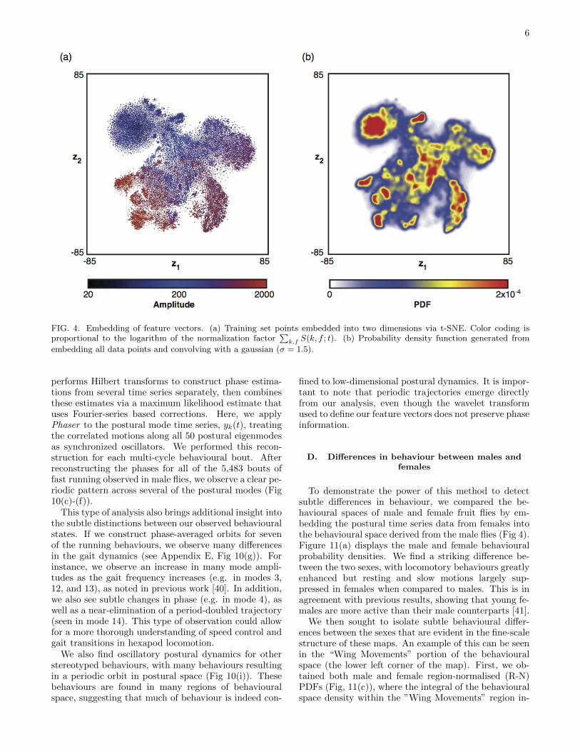
Figure 4 shows the embedding of our spectral featurevectors into two dimensions, the space (z1, z2), for all ofthe 59 individual male flies. We first note that nearbypoints have similar power (

∑k,f S(k, f ; t)), even though

the embedding algorithm normalises-out variations inthe total power of the postural motions. Embedding thesame data into three dimensions yields a very similarstructure with less than 2% reduction of the embeddingcost function (Eq. D1, Fig S3).

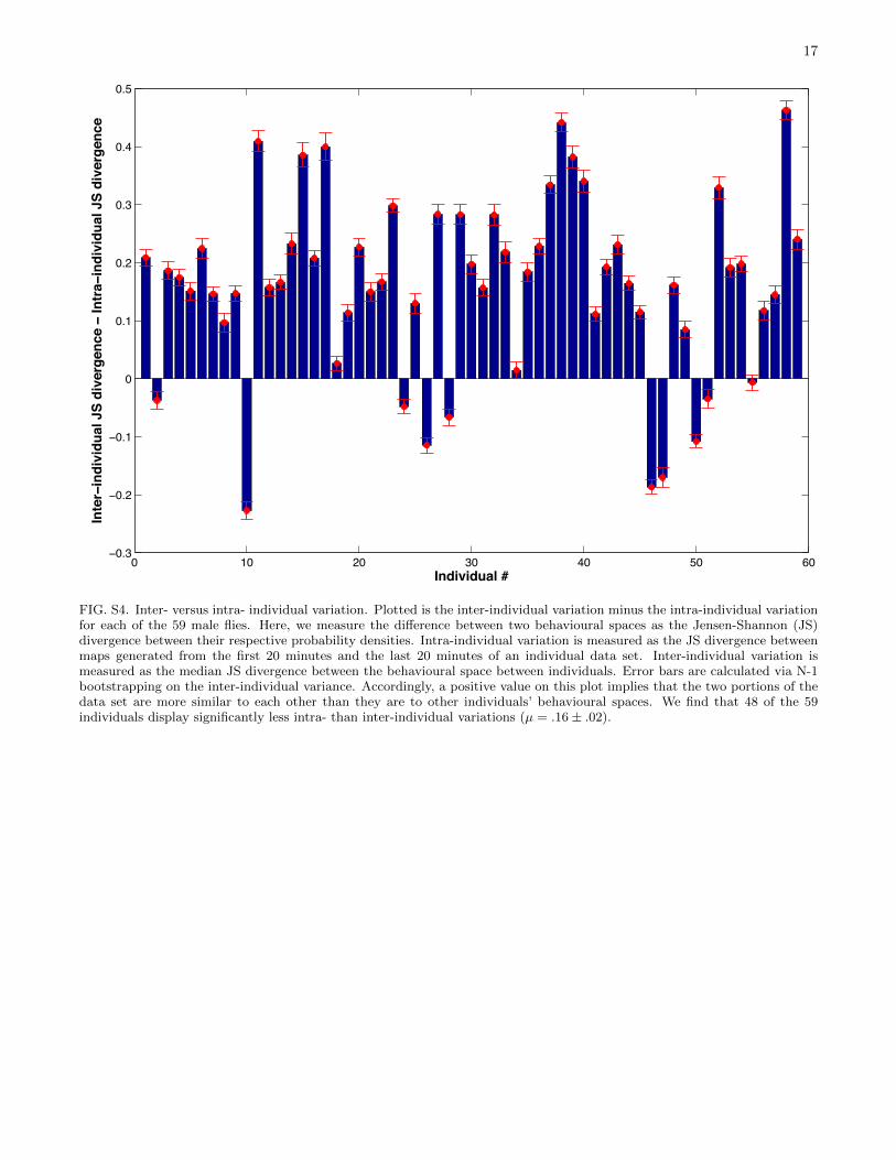
We generated an estimate of the probability density,b(z) by convolving each point in the embedded map witha gaussian of relatively small width (σ = 1.5, Fig 4(b)).Far from being uniformly distributed across this space,b(z) contains a large number of resolved local maxima.The locations of these peaks provide a potential repre-sentation for the stereotyped behaviours that the fliesperform. As expected, we find that individuals displaysignificantly less intra- than inter-individual variationwhen their behavioural maps are compared (Fig S4).

This space not only contains peaks, but the trajectorythrough it also pauses at repeatable locations. Throughnumerical differentiation of z1(t) and z2(t), we observea two-state “pause-move” pattern of dynamics. Typicaltime traces of z1(t) and z2(t) show this type of trajec-tory, with long stationary periods interspersed by quickbouts of movement (Fig 5(a)). More quantitatively, wefind that the distribution of velocities within the embed-ded space is well-represented by a two-component log-normal mixture model in which the the two peaks areseparated by almost two orders of magnitude (Fig 5(b)).The distribution of points in the low-velocity case (ap-proximately 45% of all time points) is highly localizedwith distinguishable peaks (Fig 6). The high-velocitypoints, in contrast, are more uniformly distributed.

B. Behavioural states

The embedded space is comprised of peaks surroundedby valleys. Finding connected areas in the z1, z2 planesuch that climbing up the gradient of probability densityalways leads to the same local maximum, often referredto as a watershed transform [34], we delineate 122 re-gions of the embedded space. Each of these contains asingle local maximum of probability density (Fig 7(a)).When the trajectory, z(t) pauses at one of these peaks,we find that each of these epochs correspond to the flyperforming a particular stereotyped behaviour. Thesepauses last anywhere from .05 s up to nearly 25 s (Fig8(a)).

Observing segments of the original movies correspond-ing to pauses in one of the regions, we consistently ob-serve the flies performing a distinct action that corre-sponds to a recognizable behaviour when viewed by eye(Supplementary Movies S2-11). Many of the movementswe detect are similar to familiar, intuitively defined be-havioural classifications such as walking, running, frontleg grooming, and proboscis extension, but here, the seg-mentation of the movies into behavioural categories hasemerged from the data itself, not through a priori def-initions. Moreover, we see that near-by regions of ourbehavioural space correspond to similar, yet distinct, be-haviours (Fig 7(c)).

This classification is consistent across individuals (Fig-ures 8-9, Supplementary Movies S3-11). The vast major-ity of these regions are visited by almost all of the fliesat some point (Fig 8(b)). 104 of the 122 regions werevisited by over 50 (of 59 total) flies, and the remainingbehaviours were all low-probability events, containing,in total, less than 3% of the overall activity.

C. Behavioural states as periodic orbits

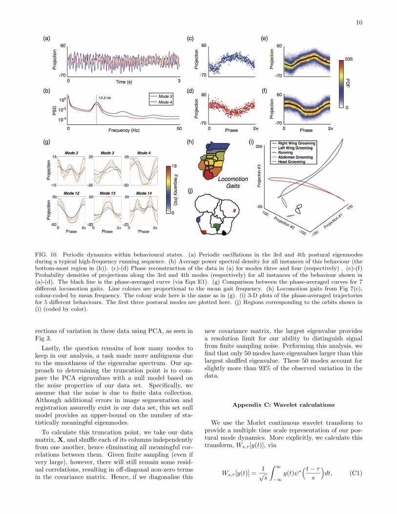
Periodic orbits in postural movements are suggestiveof underlying low-dimensional dynamic attractors thatproduce stable behavioural templates [35]. These typesof motifs have been hypothesized to form the basis forneural and mechanical control of legged locomotion atfast time scales [36]. Because our behavioural mappingalgorithm is based upon similarities between posturalfrequencies exhibited at different times, a potential hy-pothesis is that pauses in behavioural space correspondto periodic trajectories in the space of postural move-ments (Eqn 1). In our data, a fast running gait (thebottom-most region of Fig 10(h)) corresponds to peri-odic oscillations of the postural time series with a clearpeak at 12.9 Hz in the power spectral density (Fig 10(a)-(b)). This frequency is in good agreement with previousmeasurements of the fly walking gait [37, 38].

To systematically investigate the periodicity of thepostural dynamics, for each behavioural bout we maptime onto a phase variable, a cyclic coordinate definedon the unit circle. This process is usually referred to asphase reconstruction. The method we use, Phaser [39],

6

FIG. 4. Embedding of feature vectors. (a) Training set points embedded into two dimensions via t-SNE. Color coding isproportional to the logarithm of the normalization factor

∑k,f S(k, f ; t). (b) Probability density function generated from

embedding all data points and convolving with a gaussian (σ = 1.5).

performs Hilbert transforms to construct phase estima-tions from several time series separately, then combinesthese estimates via a maximum likelihood estimate thatuses Fourier-series based corrections. Here, we applyPhaser to the postural mode time series, yk(t), treatingthe correlated motions along all 50 postural eigenmodesas synchronized oscillators. We performed this recon-struction for each multi-cycle behavioural bout. Afterreconstructing the phases for all of the 5,483 bouts offast running observed in male flies, we observe a clear pe-riodic pattern across several of the postural modes (Fig10(c)-(f)).

This type of analysis also brings additional insight intothe subtle distinctions between our observed behaviouralstates. If we construct phase-averaged orbits for sevenof the running behaviours, we observe many differencesin the gait dynamics (see Appendix E, Fig 10(g)). Forinstance, we observe an increase in many mode ampli-tudes as the gait frequency increases (e.g. in modes 3,12, and 13), as noted in previous work [40]. In addition,we also see subtle changes in phase (e.g. in mode 4), aswell as a near-elimination of a period-doubled trajectory(seen in mode 14). This type of observation could allowfor a more thorough understanding of speed control andgait transitions in hexapod locomotion.

We also find oscillatory postural dynamics for otherstereotyped behaviours, with many behaviours resultingin a periodic orbit in postural space (Fig 10(i)). Thesebehaviours are found in many regions of behaviouralspace, suggesting that much of behaviour is indeed con-

fined to low-dimensional postural dynamics. It is impor-tant to note that periodic trajectories emerge directlyfrom our analysis, even though the wavelet transformused to define our feature vectors does not preserve phaseinformation.

D. Differences in behaviour between males andfemales

To demonstrate the power of this method to detectsubtle differences in behaviour, we compared the be-havioural spaces of male and female fruit flies by em-bedding the postural time series data from females intothe behavioural space derived from the male flies (Fig 4).Figure 11(a) displays the male and female behaviouralprobability densities. We find a striking difference be-tween the two sexes, with locomotory behaviours greatlyenhanced but resting and slow motions largely sup-pressed in females when compared to males. This is inagreement with previous results, showing that young fe-males are more active than their male counterparts [41].

We then sought to isolate subtle behavioural differ-ences between the sexes that are evident in the fine-scalestructure of these maps. An example of this can be seenin the “Wing Movements” portion of the behaviouralspace (the lower left corner of the map). First, we ob-tained both male and female region-normalised (R-N)PDFs (Fig, 11(c)), where the integral of the behaviouralspace density within the ”Wing Movements” region in-

7

FIG. 5. Dynamics within behavioural space. (a) Typicaltrajectory segment through behavioural space, z1(t) (blue)and z2(t) (red). (b) Histogram of velocities in the embeddedspace fit to a two-component log-gaussian mixture model.The blue bar chart represents the measured probability dis-tribution, the red line is the fitted model, and the cyan andgreen lines are the mixture components of the fitted model.

tegrates to one. Within the space of wing movements,we identified regions that show statistically significantdifferences between the two sexes using a Wilcoxon ranksum test [42] at each point in behavioural space. Thistest determines the locations of significant difference be-tween the median male PDF value and the median fe-male PDF value (p-value < .01). Regions where signifi-cant differences were found are indicated by the dashedlines in Figure 11(d).

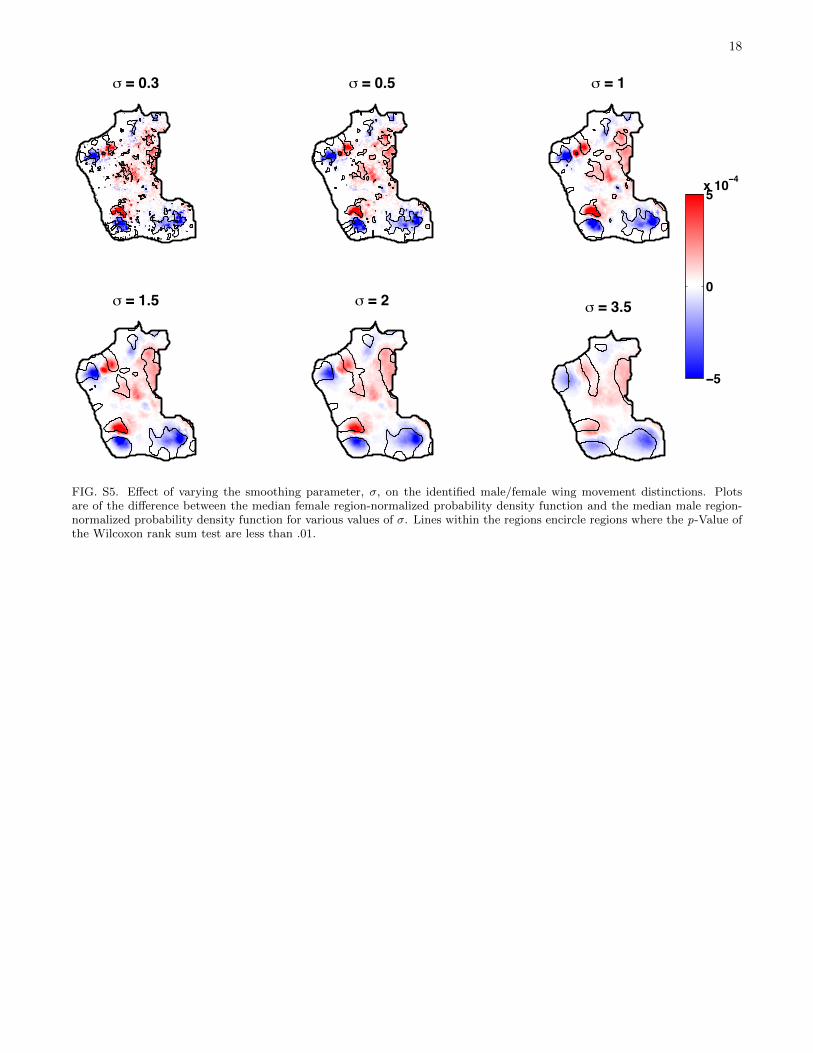
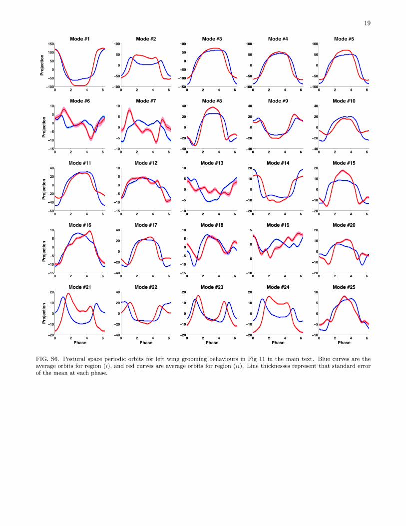
Particular behaviours, such as left-wing grooming, aresexually dimorphic (11(d) solid box, Movies S12-S13).Male-preferred grooming includes a kick of the middleleg on the left side of the body that clears the profileof the wing and moves anteriorly before pushing backtowards the posterior. Female-preferred grooming lacksthis additional leg movement. We verified this differ-ences by isolating the mean postural-space orbits asso-ciated with each of these regions (Figures 11(f), S6).Importantly, while these orbits are statistically differ-ent, the average frequencies for the behaviours are not(fmale = 3.49 ± .15 Hz versus ffemale = 3.28 ± .08 Hz).We note that these results are consistent across a largerange of the behavioural-map smoothing parameter σ

(Fig S5), such that fine-tuning of the spatial structureof the behavioural map is not necessary to obtain theresults seen here.

It should be noted that future study is necessary todetermine the ethological relevance of these findings andto understand how much of the variance we observe isrelated to the specifics of our experimental paradigm.However, the fact that these distinctions are found with-out specifically looking for any of them – emerging onlyfrom underlying statistics of the behavioural map – pro-vides quantitative verification that the classifications wemake are meaningful. Inherent in any unsupervised clas-sification method is the question of how to validate itsaccuracy. Here, there is no ground truth with whichto compare, since a significant aim of our work is todispense with a priori behavioural definitions. How-ever, by showing that meaningful distinctions and ag-glomerations can be made between different behaviouralinstances, we provide evidence that the approach intro-duced here can become the basis undergirding a widerange of experimental investigations into the behaviourof animals.

V. CONCLUSIONS

The ability to map and compare the behaviouralrepertoire of individuals and populations of animals hasapplications beyond the study of terrestrial dynamics infruit flies. Combined with tools for genetic manipulation,DNA sequencing, neural imaging, and electrophysiology,the identification of subtle behavioural distinctions andpatterns between groups of individuals will impact deepquestions related to the interactions between genes, neu-rons, behaviour, and evolution. In this initial study, weprobed the motion of individuals in a largely feature-less environment. Extensions to more complicated situ-ations, e.g. where sensory inputs are measured and/orcontrolled, genes are manipulated, or multiple individu-als are present, are readily implemented.

Finally, we note that the only Drosophila-specific stepin our analysis pipeline is the generation of the postu-ral eigenmodes. Given movies of sufficient quality andlength from different organisms, spectral feature vectorsand behavioural spaces can be similarly generated, al-lowing for potential applications from worms to mice tohumans and a greater understanding of how animals be-have.

ACKNOWLEDGEMENTS

We thank Yi Deng, Kieren James-Lubin, Kelsi Lind-blad, and Ugne Klibaite for assistance in data collectionand analysis, as well as Jessica Cande, David Stern, andDavid Schwab for discussions and suggestions. JWS andGJB also acknowledge the Howard Hughes Medical Insti-tute Janelia Farm Visitor Program and the Aspen Centerfor Physics, where many ideas for this work were formu-

8

FIG. 6. Concentration of behavioural space during stereotyped movements. Comparison between the densities generatedduring stereotyped (a) and non-stereotyped (b) epochs.

FIG. 7. Segmentation into behavioural regions. (a) Boundary lines obtained from performing a watershed transform on thePDF from Fig 4(b). (b) Integrated probabilities within each of the regions. (c) The organisation of behavioural space intoregions of similar movement types. Definition of regions is performed through visual assessment of movies.

lated. This work was funded through awards from theNational Institutes of Health (GM098090, GM071508),The National Science Foundation (PHY–0957573, PHY–1066293), the Pew Charitable Trusts, the Swartz Foun-dation, and the Alfred P. Sloan Foundation.

DATA ACCESSIBILITY

Example code for running the algorithms can be foundat https://github.com/gordonberman/MotionMapper.For access to raw image data, please email JWS at shae-vitz@princeton.edu.

APPENDICES

Appendix A: Image processing

To isolate the fly from the background, we applyCanny’s method for edge detection [19], resulting in a bi-nary image containing the edge positions. We then mor-phologically dilate this binary image by a 3×3 square inorder to fill any spurious holes in the edges and proceedto fill all closed curves. This filled image is then morpho-logically eroded by a square of the same size, resulting ina mask. After applying this mask to the original image,we now have our segmented image.

9

FIG. 8. Behavioural state dynamics. (a) Distribution of oc-cupancy times in all behaviours. (b) Number of individuals(out of 59 possible) that visit each behaviour at some pointduring observation.

While our tracking algorithm ensures that the fly re-mains within the image boundaries, the centre of thefly and the orientation within the frame vary over time.Having obtained a sequence of isolated fly images, wenext register them both translationally and rotationallywith respect to a template image. The template imageis generated by taking a typical image of a fly and thenmanually ablating the wings and legs digitally.

For our first step, we rotationally align. This isachieved through finding the angle that maximises thecross-correlation between the magnitudes of the 2D po-lar Fourier transforms for each image and the template.Because all translation information appears in the phaseof the 2D Fourier transform, this rotational alignment,based only upon the magnitude of the transform, is inde-pendent of any initial translations between the images.Accordingly, once rotational alignment is achieved, wecan subsequently register the images translationally viaa cross-correlation.

FIG. 9. Behavioural space peaks correspond to specificstereotyped behaviours. Selected regions within behaviouralspace are shown and are labeled via the colour-coded legendon the right. Instances of dwells within each of these regionscan be seen in Supplementary Movies 3-11. The examplesdisplayed in these movies are randomly selected and containclips from many different flies, showing that the behaviouralspace provides a representation of behaviour that is consis-tent across individuals.

Appendix B: Postural decomposition from images

The aim of the postural decomposition is to take ourset of 200 × 200 aligned images and create a lower-dimensional representation that can be made into timeseries. Naively, one would simply perform PCA on thethe images, using each pixel value as a separate dimen-sion. The fly images, however, contain too many pixelsto analyse due to memory limitations.

To make this problem more tractable, we analyse onlythe subset of these pixels which have non-negligible vari-ance. Many pixels within the fly image are either al-ways zero or always saturated, thus containing almostno dynamical information. Accordingly, we would liketo use only a subsample of these measurements. Themost obvious manner to go about this is to find the pix-els containing the highest variance and keep only thoseabove a certain threshold. The primary difficulty here,however, is that there is not an obvious truncation point(Fig S2A). This is most likely the result of the fact thatthe fly legs can potentially occupy the majority of thepixels in the image but only are present in a relativelysmall number in any given frame. Hence, many of theseperiphery pixels all have similarly moderate standard de-viations, making them difficult to differentiate.

A more compact scheme is to represent the imagesin Radon-transform space, which more sparsely param-eterises lines such as legs or wing veins. After Radontransformation, the probability density function of pixel-value standard deviations has a clear minimum and wekeep pixels whose standard deviation is larger than thisvalue (Fig S2B). This results in keeping 6,763 pixels outof 18,090, retaining approximately 95% of the total vari-ation in the images. If there are N images in our sample,we can represent our data set, X as an N×6, 763-elementmatrix. We then proceed to calculate the principal di-

10

FIG. 10. Periodic dynamics within behavioural states. (a) Periodic oscillations in the 3rd and 4th postural eigenmodesduring a typical high-frequency running sequence. (b) Average power spectral density for all instances of this behaviour (thebottom-most region in (h)). (c)-(d) Phase reconstruction of the data in (a) for modes three and four (respectively) . (e)-(f)Probability densities of projections along the 3rd and 4th modes (respectively) for all instances of the behaviour shown in(a)-(d). The black line is the phase-averaged curve (via Eqn E1). (g) Comparison between the phase-averaged curves for 7different locomotion gaits. Line colours are proportional to the mean gait frequency. (h) Locomotion gaits from Fig 7(c),colour-coded by mean frequency. The colour scale here is the same as in (g). (i) 3-D plots of the phase-averaged trajectoriesfor 5 different behaviours. The first three postural modes are plotted here. (j) Regions corresponding to the orbits shown in(i) (coded by color).

rections of variation in these data using PCA, as seen inFig 3.

Lastly, the question remains of how many modes tokeep in our analysis, a task made more ambiguous dueto the smoothness of the eigenvalue spectrum. Our ap-proach to determining the truncation point is to com-pare the PCA eigenvalues with a null model based onthe noise properties of our data set. Specifically, weassume that the noise is due to finite data collection.Although additional errors in image segmentation andregistration assuredly exist in our data set, this set nullmodel provides an upper-bound on the number of sta-tistically meaningful eigenmodes.

To calculate this truncation point, we take our datamatrix, X, and shuffle each of its columns independentlyfrom one another, hence eliminating all meaningful cor-relations between them. Given finite sampling (even ifvery large), however, there will still remain some resid-ual correlations, resulting in off-diagonal non-zero termsin the covariance matrix. Hence, if we diagonalise this

new covariance matrix, the largest eigenvalue providesa resolution limit for our ability to distinguish signalfrom finite sampling noise. Performing this analysis, wefind that only 50 modes have eigenvalues larger than thislargest shuffled eigenvalue. These 50 modes account forslightly more than 93% of the observed variation in thedata.

Appendix C: Wavelet calculations

We use the Morlet continuous wavelet transform toprovide a multiple time scale representation of our pos-tural mode dynamics. More explicitly, we calculate thistransform, Ws,τ [y(t)], via

Ws,τ [y(t)] =1√s

∫ ∞−∞

y(t)ψ∗( t− τ

s

)dt, (C1)

11

FIG. 11. Comparison between male and female behaviours. (a) Measured behavioural space PDF for male (left) and female(right) flies. (b) Difference between the two PDFs in (a). Here we observe large dimorphisms between the sexes, particularlyin the ”Locomotion Gaits” and ”Idle and Slow Movements” regions. (c) PDFs for behaviours in the “Wing Movements”portion of the behavioural space (the lower left of the full space). These PDFs (male on the left and female on the right) arenormalised so that they each integrate to one. The black lines are the boundaries found from a watershed transform and areincluded to guide the eye. (d) Difference between the two normalised behavioural spaces in (c). Dashed lines enclose regions inwhich the median male and the median female PDF values are statistically different via the Wilcoxan rank sum test (p < .01).(e) Zoom-in on the boxed region in (d). Both of these regions correspond to left wing grooming, but with behaviours withinthe male-preferred region incorporating an additional leg kick (Supplementary Movies S12-13). (f) Average periodic orbits forpostural eigenmodes 1, 2, 6, and 7. The area surrounding the lines represents the standard error of the mean at each pointalong the trajectory. Average periodic orbits for all of the first 25 postural modes are shown in Fig S6.

with

ψ(η) = π−1/4eiω0ηe−12η

2

. (C2)

Here, yi(t) is a postural time series, s is the time scale ofinterest, τ is a point in time, and ω0 is a non-dimensionalparameter (set to 5 here).

The Morlet wavelet has the additional property thatthe time scale, s, is related to the Fourier frequency, f ,

by

s(f) =ω0 +

√2 + ω2

0

4πf. (C3)

This can be derived by maximizing the response to a

pure sine wave, A(s, f) ≡∣∣∣Ws,τ [e2πift]

∣∣∣, with respect tos.

However, A(s, ω) is disproportionally large when re-sponding to pure sine waves of lower frequencies. To

12

correct for this, we find a scalar function C(s) such that

C(s)A(s, ω∗) = 1 for all s, (C4)

where ω∗ is 2π times the Fourier frequency found in Eq.C3. For a Morlet wavelet, this function is

C(s) =π−

14

√2se

14

(ω0−√ω2

0+2

)2

. (C5)

Accordingly, we can define our power spectrum,S(k, f ; t), via

S(k, f ; τ) =1

C(s(f))

∣∣∣Ws(f),τ [yk(t)]∣∣∣ (C6)

Last, we use a dyadically-spaced set of frequencies be-tween fmin = 1 Hz and the Nyquist frequency (fmax =50 Hz) via

fi = fmax2−(i−1)/(Nf−1) log2

fmaxfmin (C7)

for i = 1, 2, . . . , Nf (and their corresponding scales viaEq. C3). This creates a wavelet spectrogram that isresolved at multiple time-scales for each of the first 50postural modes.

Appendix D: t-SNE implementation

For our initial embedding using t-SNE, we largely fol-low the method introduced in [18], minimizing the costfunction

C = DKL(P ||Q) =∑ij

pij logpijqij, (D1)

where pij = 12 (pj|i + pi|j),

qij =(1 + ∆2

ij)−1∑

k

∑` 6=k(1 + ∆2

k,`)−1 , (D2)

and ∆ij is the Euclidean distance between points i andj in the embedded space. The cost function is optimisedthrough a gradient descent procedure that is precededby an early-exaggeration period, allowing for the systemto more readily escape local minima.

The memory complexity of this algorithm prevents thepractical number of points from exceeding ≈ 35, 000. Al-though improving this number is the subject of currentresearch [43], our solution here is to generate an embed-ding using a selection of roughly 600 data points fromeach of the 59 individuals observed (out of ≈ 360, 000data points per individual). To ensure that these pointscreate a representative sample, we perform t-SNE on20,000 randomly-selected data points from each individ-ual. This embedding is then used to estimate a probabil-ity density by convolving each point with a 2D gaussianwhose whose width is equal to the distance from thepoint to its Nembed = 10 nearest neighbours. This space

is segmented by applying a watershed transform [34] tothe inverse of the PDF, creating a set of regions. Finally,points are grouped by the region to which they belongand the number of points selected out of each region isproportional to the integral over the PDF in that re-gion. This is performed for all data sets, yielding a totalof 35,000 data points in the training set.

Given the embedding resulting from applying t-SNEto our training set, we wish to embed additional pointsinto our behavioural space by comparing each to thetraining set individually. Mathematically, let X be theset of all feature vectors in the training set, X ′ be theirassociated embeddings via t-SNE, z be a new featurevector that we would like to embed according to themapping between X and X ′, and ζ be the embedding ofz that we would like to determine.

As with the t-SNE cost function, we will embed zby enforcing that its transition probabilities in the twospaces are as similar as possible. Like before, the tran-sitions in the full space, pj|z, are given by

pj|z =exp(− d(z, j)2/2σ2

z

)∑x∈X exp

(− d(z, k)2/2σ2

z

) , (D3)

where d(z, j) is the Kullback-Leibler divergence betweenz and x ∈ X, and σz is once again found by constrainingthe entropy of the condition transition probability dis-tribution, using the same parameters as for the t-SNEembedding. Similarly, the transition probabilities in theembedded space are given by

qj|ζ =(1 + ∆2

ζ,j)−1∑

x′∈X′(1 + ∆2ζ,x′)−1

, (D4)

where ∆ζ,x′ is the Euclidean distance between ζ and y ∈X ′.

For each z, we then seek the ζ∗ that minimisesthe Kullback-Leibler divergence between the transitionprobability distributions in the two spaces:

ζ∗ = arg minζDKL(px|z||qy|ζ) (D5)

= arg minζ

∑x∈X

px|z logpx|z

qy(x)|ζ. (D6)

As before, this is a non-convex function, leading to po-tential complexities in performing our desired optimiza-tion. However, if we start a local optimization (us-ing the Nelder-Mead Simplex algorithm [44, 45]) froma weighted average of points, ζ0, where

ζ0 =∑x∈X

px|zy(x), (D7)

this point is almost always within the basin of attractionof the global minimum. To ensure that this is true in allcases, however, we also perform the same minimisationprocedure, but starting from the point y(x∗), where

x∗ = arg maxx

px|z. (D8)

13

This returned a better solution approximately 5% of thetime.

Because this embedding can be calculated indepen-dently for each value of z, the algorithm scales linearlywith the number of points. We also make use of thefact that this algorithm is embarrassingly parallelizable.Moreover, because we have set our transition entropy,H, to be equal to 5, there are rarely more than 50 pointsto which a given z has a non-zero transition probability.Accordingly, we can speed up our cost function eval-uation considerably by only allowing px|z > 0 for thenearest 200 points to z in the original space.

Lastly, we find the space of behaviours for the femaledata sets by embedding these data into the space cre-ated with the male training set. We find that the me-dian re-embedding cost (Eqn. D5) for the female costis only 1% more than the median re-embedding cost forthe male data (5.08 bits vs. 5.12 bits) indicating thatthe embedding works well for both sexes.

Appendix E: Phase-averaged orbits

After applying the Phaser algorithm, we find thephase-averaged orbit via a von Mises distributionweighted average. More precisely, we construct the av-erage orbit for eigenmode k, µ(k)(φ) via

µ(k)(φ) =∑i

y(k)i

exp[κ cos(φ− φi)]∑j exp[κ cos(φ− φj)]

, (E1)

where y(k)i is the projection onto the kth eigenmode at

time point ti, φi is the phase associated with the sametime point, and κ is related to the standard deviation of

the von Mises distribution (σ2vM (κ) = 1 − I1(κ)

I0(κ), where

Iν(x) is the modified Bessel function of νth order). Herewe find the value of κ ≈ 50.3, which is the κ resulting inσvM = .1.

Because phase reconstruction only is unique up toan additive constant, to compare phase-averaged curvesof different behavioural bouts, an additional alignmentneeds to occur. This is performed by first finding themaximum value of cross-correlation between the phase-averaged curves for each mode. Then, the phase offsetbetween that pair of 50-dimensional orbits is given bythe median of these found phase shifts.

14

Appendix F: Supplementary Tables

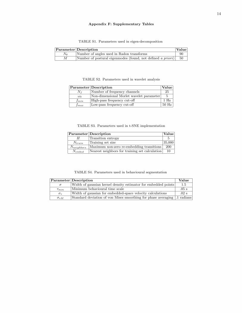
TABLE S1. Parameters used in eigen-decomposition

Parameter Description ValueNθ Number of angles used in Radon transforms 90M Number of postural eigenmodes (found, not defined a priori) 50

TABLE S2. Parameters used in wavelet analysis

Parameter Description ValueNf Number of frequency channels 25ω0 Non-dimensional Morlet wavelet parameter 5fmin High-pass frequency cut-off 1 Hzfmax Low-pass frequency cut-off 50 Hz

TABLE S3. Parameters used in t-SNE implementation

Parameter Description ValueH Transition entropy 5

Ntrain Training set size 35,000Nneighbors Maximum non-zero re-embedding transitions 200Nembed Nearest neighbors for training set calculation 10

TABLE S4. Parameters used in behavioural segmentation

Parameter Description Valueσ Width of gaussian kernel density estimator for embedded points 1.5

τmin Minimum behavioural time scale .05 sσv Width of gaussian for embedded-space velocity calculations .02 sσvM Standard deviation of von Mises smoothing for phase averaging .1 radians

15

Appendix G: Supplementary Figures

0 10 20 30 40 50 600

0.5

1

1.5

2

2.5

3

Time (minutes)

Velo

city

(mm

/s)

FIG. S1. Flies adapt to the arena in about five minutes. Median movement velocity for male flies (N = 59) during the65 minute filming period. Pink regions represent the 25% and 75% quantiles at each point in time. Note that almost alladaptation occurs within the first five minutes placed in the dish. This region is excluded from our analyses

16

FIG. S2. Radon vs. pixel representation of images. A) Probability density function of pixel standard deviations. B)Probability density function of Radon pixel standard deviations. Note the clear minimum that exists in B), allowing for aneffective reduction in the number of pixels necessary to represent the data.

FIG. S3. Comparison between embedding into 3-D (A) versus 2-D (B) via t-SNE. Other than the embedding dimension, allother parameters remain constant. Color labels are proportional to the logarithm of the normalizing amplitude (

∑k,f S(k, f ; t))

for each point in the training set. There is a 2% improvement in the error function (Equation D1) in the 3-D case as comparedto the 2-D embedding (2.9 versus 3.3 bits out of a total of 20.6 bits for the transition matrix P ).

17

0 10 20 30 40 50 60−0.3

−0.2

−0.1

0

0.1

0.2

0.3

0.4

0.5

Individual #

Inte

r−in

divi

dual

JS

dive

rgen

ce −

Intr

a−in

divi

dual

JS

dive

rgen

ce

FIG. S4. Inter- versus intra- individual variation. Plotted is the inter-individual variation minus the intra-individual variationfor each of the 59 male flies. Here, we measure the difference between two behavioural spaces as the Jensen-Shannon (JS)divergence between their respective probability densities. Intra-individual variation is measured as the JS divergence betweenmaps generated from the first 20 minutes and the last 20 minutes of an individual data set. Inter-individual variation ismeasured as the median JS divergence between the behavioural space between individuals. Error bars are calculated via N-1bootstrapping on the inter-individual variance. Accordingly, a positive value on this plot implies that the two portions of thedata set are more similar to each other than they are to other individuals’ behavioural spaces. We find that 48 of the 59individuals display significantly less intra- than inter-individual variations (µ = .16 ± .02).

18

m = 0.3 m = 0.5 m = 1

m = 1.5 m = 2 m = 3.5

−5

0

5x 10−4

FIG. S5. Effect of varying the smoothing parameter, σ, on the identified male/female wing movement distinctions. Plotsare of the difference between the median female region-normalized probability density function and the median male region-normalized probability density function for various values of σ. Lines within the regions encircle regions where the p-Value ofthe Wilcoxon rank sum test are less than .01.

19

0 2 4 6−100

−50

0

50

100

150Mode #1

Proj

ectio

n

0 2 4 6−100

−50

0

50

100Mode #2

0 2 4 6−150

−100

−50

0

50

100Mode #3

0 2 4 6−100

−50

0

50

100Mode #4

0 2 4 6−100

−50

0

50

100Mode #5

0 2 4 6−15

−10

−5

0

5

10Mode #6

Proj

ectio

n

0 2 4 6−10

−5

0

5

10Mode #7

0 2 4 6−40

−20

0

20

40Mode #8

0 2 4 6−40

−20

0

20

40Mode #9

0 2 4 6−40

−20

0

20

40Mode #10

0 2 4 6−60

−40

−20

0

20

40Mode #11

Proj

ectio

n

0 2 4 6−15

−10

−5

0

5

10Mode #12

0 2 4 6−10

−5

0

5

10Mode #13

0 2 4 6−20

−10

0

10

20Mode #14

0 2 4 6−20

−10

0

10

20Mode #15

0 2 4 6−15

−10

−5

0

5

10Mode #16

Proj

ectio

n

0 2 4 6−40

−20

0

20

40Mode #17

0 2 4 6−15

−10

−5

0

5

10Mode #18

0 2 4 6−10

−5

0

5Mode #19

0 2 4 6−20

−10

0

10

20Mode #20

0 2 4 6−20

−10

0

10

20Mode #21

Proj

ectio

n

Phase0 2 4 6

−40

−20

0

20

40Mode #22

Phase0 2 4 6

−20

−10

0

10

20Mode #23

Phase0 2 4 6

−20

−10

0

10

20Mode #24

Phase0 2 4 6

−10

−5

0

5

10Mode #25

Phase

FIG. S6. Postural space periodic orbits for left wing grooming behaviours in Fig 11 in the main text. Blue curves are theaverage orbits for region (i), and red curves are average orbits for region (ii). Line thicknesses represent that standard errorof the mean at each phase.

20

Appendix H: Supplementary Movie Legends

Supplementary movies can be obtained by emailing GJB (gberman@princeton.edu)

Movie S1. Raw video data of a behaving fly (left) and the corresponding segmented and aligned data (right).Movie S2. Dynamics in behavioural space. Raw video of a behaving D. melanogaster (middle) is displayed alongsidecoordinates of the fly’s position within the filming apparatus (left) and its position in the embedded behaviouralspace (right). The red circles represent the positions in the appropriate coordinate system and the trailing lines arethe positions traversed in the previous .5 s. The light blue shading indicates that a particular behaviour is beingperformed, and the blue text below the video of the fly gives a coarse label for the behaviour. The first portion ofthe movie is 5 s, played at real time (indicated by “Real Time” above the fly video), and the subsequent portion ofthe movie is slowed down by a factor of 5 for clarity (indicated by “Slowed 5×”).Movies S3-11. Each movie is a mosaic of multiple instances of specific regions in behavioural space as displayedin Fig 9 and Table S5. Every movie contains multiple segments from many different individuals and are slowed by afactor of 4 for clarity.

TABLE S5. Behavioural Movies

Movie LabelMovie S3 IdleMovie S4 Right wing groomingMovie S5 Left wing groomingMovie S6 Left wing and legs groomingMovie S7 Wing waggleMovie S8 Abdomen groomingMovie S9 RunningMovie S10 Front leg groomingMovie S11 Head grooming

Movie S12. Composite movie (slowed by a factor of 4) of randomly chosen instances of flies from the male-preferredbehavioural region in Fig 11 of the main text.Movie S13. Composite movie (slowed by a factor of 4) of randomly chosen instances of flies from the female-preferredbehavioural region in Fig 11 of the main text.

REFERENCES

[1] Altmann, J., 1974 Observational Study of Behavior: Sampling Methods. Behaviour 49, 227–267.[2] Lehner, P. A., 1996 Handbook of ethological methods. Cambridge, UK: Cambridge University Press, 2nd edition.[3] Gould, J. L., 1982 Ethology: The Mechanisms and Evolution of Behavior. New York, NY: W. W. Norton & Company.[4] Stephens, G. J., Osborne, L. C. & Bialek, W., 2011 Searching for simplicity in the analysis of neurons and behavior. Proc.

Nat. Acad. Sci. 108, 15565–15571. (doi:10.1073/pnas.1010868108).[5] Glimcher, P. W. & Dorris, M., 2004 Neuronal studies of decision making in the visual-saccadic system. In The Cognitive

Neurosciences III (ed. M. S. Gazzaniga), pp. 1215–1228. MIT Press.[6] Manoli, D. S., Meissner, G. W. & Baker, B. S., 2006 Blueprints for behavior: genetic specification of neural circuitry for

innate behaviors. Trends In Neurosciences 29, 444–451. (doi:10.1016/j.tins.2006.06.006).[7] Osborne, L. C., Lisberger, S. G. & Bialek, W., 2005 A sensory source for motor variation. Nature 437, 412–416. (doi:

10.1038/nature03961).[8] Stephens, G. J., Johnson-Kerner, B., Bialek, W. & Ryu, W. S., 2008 Dimensionality and dynamics in the behavior of C.

elegans. PLoS Comp. Bio. 4, e1000028. (doi:10.1371/journal.pcbi.1000028).[9] Stephens, G. J., de Mesquita, M. B., Ryu, W. S. & Bialek, W., 2011 Emergence of long timescales and stereotyped

behaviors in Caenorhabditis elegans. Proc. Nat. Acad. Sci. 108, 7286–7289. (doi:10.1073/pnas.1007868108).[10] Desrochers, T. M., Jin, D. Z., Goodman, N. D. & Graybiel, A. M., 2010 Optimal habits can develop spontaneously

through sensitivity to local cost. Proc. Nat. Acad. Sci. 107, 20512–20517. (doi:10.1073/pnas.1013470107).[11] Brown, A. E. X., Yemini, E. I., Grundy, L. J., Jucikas, T. & Schafer, W. R., 2013 A dictionary of behavioral mo-

tifs reveals clusters of genes affecting caenorhabditis elegans locomotion. Proc. Nat. Acad. Sci. 110, 791–796. (doi:10.1073/pnas.1211447110).

[12] Dankert, H., Wang, L., Hoopfer, E. D., Anderson, D. J. & Perona, P., 2009 Automated monitoring and analysis of socialbehavior in Drosophila. Nature Methods 6, 297–303. (doi:10.1038/nmeth.1310).

21

[13] Branson, K., Robie, A. A., Bender, J., Perona, P. & Dickinson, M. H., 2009 High-throughput ethomics in large groups ofDrosophila. Nature Methods 6, 451–457. (doi:10.1038/nmeth.1328).

[14] Kabra, M., Robie, A. A., Rivera-Alba, M., Branson, S. & Branson, K., 2013 JAABA: interactive machine learning forautomatic annotation of animal behavior. Nature Methods 10, 64–67. (doi:10.1038/nmeth.2281).

[15] de Chaumont, F., Coura, R. D.-S., Serreau, P., Cressant, A., Chabout, J., Granon, S. & Olivo-Marin, J.-C., 2012Computerized video analysis of social interactions in mice. Nature Methods 9, 410–417. (doi:10.1038/nmeth.1924).

[16] Kain, J., Stokes, C., Gaudry, Q., Song, X., Foley, J., Wilson, R. & de Bivort, B., 2013 Leg-tracking and automatedbehavioural classification in Drosophila. Nature Communications 4, 1910. (doi:10.1038/ncomms2908).

[17] Simon, J. C. & Dickinson, M. H., 2010 A new chamber for studying the behavior of Drosophila. PLoS ONE 5, e8793.(doi:10.1371/journal.pone.0008793).

[18] van der Maaten, L. & Hinton, G., 2008 Visualizing data using t-SNE. J. Mach. Learning Research 9, 85.[19] Canny, J., 1986 A computational approach to edge detection. IEEE Trans Pattern Analysis and Machine Intelligence 8,

679–714. (doi:10.1109/TPAMI.1986.4767851).[20] De Castro, E. & Morandi, C., 1987 Registration of translated and rotated images using finite Fourier transforms. IEEE

Trans on Pattern Anal and Mach Int 5, 700–703.[21] Reddy, B. S. & Chatterji, B. N., 1996 An FFT-based technique for translation, rotation, and scale-invariant image

registration. IEEE Trans on Image Processing 5, 1266–1271. (doi:10.1109/83.506761).[22] Wilson, C. A. & Theriot, J. A., 2006 A correlation-based approach to calculate rotation and translation of moving cells.

IEEE Trans on Image Processing 15, 1939–1951. (doi:10.1109/TIP.2006.873434).[23] Guizar-Sicairos, M. & Thurman, S. T., 2008 Efficient subpixel image registration algorithms. Opt Lett 33, 156–158.

(doi:10.1364/OL.33.000156).[24] Revzen, S. & Guckenheimer, J. M., 2012 Finding the dimension of slow dynamics in a rhythmic system. Journal of the

Royal Society Interface 9, 957–971. (doi:10.1098/rsif.2011.0431).[25] Ristroph, L., Berman, G. J., Bergou, A. J., Wang, Z. J. & Cohen, I., 2009 Automated hull reconstruction motion tracking

(HRMT) applied to sideways maneuvers of free-flying insects. J Exp Bio 212, 1324–1335. (doi:10.1242/jeb.025502).[26] Fontaine, E. I., Zabala, F., Dickinson, M. H. & Burdick, J. W., 2009 Wing and body motion during flight initiation in

Drosophila revealed by automated visual tracking. J Exp Bio 212, 1307–1323. (doi:10.1242/jeb.025379).[27] Ye, L. & Keogh, E., 2011 Time series shapelets: a novel technique that allows accurate, interpretable and fast classification.

Data Mining and Knowledge Discovery 22, 149–182. (doi:10.1007/s10618-010-0179-5).[28] Goupillaud, P., Grossman, A. & Morlet, J., 1984 Cycle-octave and related transforms in seismic signal analysis. Geoex-

ploration 23, 85–102.[29] Daubechies, I., 1992 Ten Lectures on Wavelets. Philadelphia, PA: SIAM.[30] Cox, T. F. & Cox, M. A. A., 2000 Multidimensional Scaling. Boca Raton, FL: Chapman and Hall, 2 edition.[31] Tenenbaum, J. B., de Silva, V. & Langford, J. C., 2000 A global geometric framework for nonlinear dimensionality

reduction. Science 290, 2319–2323. (doi:10.1126/science.290.5500.2319).[32] Roweis, S. T. & Saul, L. K., 2000 Nonlinear dimensionality reduction by locally linear embedding. Science 290, 2323–2326.

(doi:10.1126/science.290.5500.2323).[33] Cover, T. M. & Thomas, J. A., 2006 Elements of Information Theory. Hoboken, NJ: Wiley-Interscience, 2nd edition.[34] Meyer, F., 1994 Topographic distance and watershed lines. Signal Processing 38, 113–125.[35] Full, R. J. & Koditschek, D. E., 1999 Templates and anchors: neuromechanical hypotheses of legged locomotion on land.

Journal of Experimental Biology 202, 3325–3332.[36] Holmes, P., Full, R. J., Koditschek, D. & Guckenheimer, J., 2006 The dynamics of legged locomotion: Models, analyses,

and challenges. Siam Review 48, 207–304. (doi:10.1137/S0036144504445133).[37] Strauss, R. & Heisenberg, M., 1990 Coordination of legs during straight walking and turning in Drosophila melanogaster.

J Comp Physiol A 167, 403–412.[38] Wosnitza, A., Bockemuhl, T., Dubbert, M., Scholz, H. & Buschges, A., 2013 Inter-leg coordination in the control of

walking speed in Drosophila. Journal of Experimental Biology 216, 480–491. (doi:10.1242/jeb.078139).[39] Revzen, S. & Guckenheimer, J. M., 2008 Estimating the phase of synchronized oscillators. Phys Rev E 78, 051907.

(doi:10.1103/PhysRevE.78.051907).[40] Mendes, C. S., Bartos, I., Akay, T., Marka, S. & Mann, R. S., 2013 Quantification of gait parameters in freely walking

wild type and sensory deprived Drosophila melanogaster. eLife 2, e00231–e00231. (doi:10.7554/eLife.00231.027).[41] Le Bourg, E., 1987 The rate of living theory. Spontaneous locomotor activity, aging and longevity in Drosophila

melanogaster. Experimental gerontology 22, 359–369.[42] Wilcoxon, F., 1945 Individual comparisons by ranking methods. Biometrics Bulletin 1, 80–83.[43] van der Maaten, L., 2013 Barnes-Hut-SNE. arXiv p. 1301.3342.[44] Jongen, H. T., Meer, K. & Triesch, E., 2004 Optimization Theory. Boston, MA: Kluwer Academic Publishers.[45] Lagarias, J. C., Reeds, J. A., Wright, M. H. & Wright, P. E., 1998 Convergence properties of the nelder-mead simplex

method in low dimensions. SIAM J. Optim. 9, 112–147.