GEOLOGICAL SURVEY OF CANADA

OPEN FILE 7689

Principal Component Analysis of Geochemical Data from the

REE-rich Maw Zone, Athabasca Basin, Canada

S. Chen, E.C. Grunsky, K. Hattori and Y. Liu

2015

GEOLOGICAL SURVEY OF CANADA

OPEN FILE 7689

Principal Component Analysis of Geochemical Data from the

REE-rich Maw Zone, Athabasca Basin, Canada

S. Chen1, E.C. Grunsky2, K. Hattori1 and Y. Liu3

1 Dept. Earth Sciences, University of Ottawa, 25 Templeton Street, Ottawa, Ontario

2 Geological Survey of Canada, 601 Booth Street, Ottawa, Ontario

3 Denison Mines Corporation, 230 22nd Street. East, Suite 200, Saskatoon, Saskatchewan

2015

© Her Majesty the Queen in Right of Canada, as represented by the Minister of Natural Resources Canada, 2015

doi:10.4095/295615

This publication is available for free download through GEOSCAN (http://geoscan.nrcan.gc.ca/).

Recommended citation

Chen, S., Grunsky, E.C., Hattori, K., and Liu, Y., 2015. Principal Component Analysis of Geochemical Data from the

REE-rich Maw Zone, Athabasca Basin, Canada; Geological Survey of Canada, Open File 7689, 24p.

doi:10.4095/295615

Publications in this series have not been edited; they are released as submitted by the author.

Table of Contents

Abstract .................................................................................................................................................... 1

Introduction .............................................................................................................................................. 2

Selection of suitable type of PCA ............................................................................................................ 2

Application of RQ- PCA to Geochemical Data ....................................................................................... 3

Geology of the Maw Zone ....................................................................................................................... 3

Application of PCA to the Maw Zone Geochemical Data ...................................................................... 5

Summary ................................................................................................................................................ 12

Acknowledgements ................................................................................................................................ 13

References .............................................................................................................................................. 14

Appendix. The Closure Problem............................................................................................................ 20

1

Abstract

Elemental assemblages derived from geochemical data are produced by geological processes, such as

alteration and mineralization. However, processing large amounts of geochemical data that may reflect

a variety of geochemical processes, can be a challenge. Methods such as principal component analysis

(PCA) can be used to reduce the number of observed variables into a smaller number of artificial

variables that account for most of the variance in a given dataset. This study uses RQ-mode PCA,

which computes variable and object loadings simultaneously and displays the observations and the

variables at the same scale.

In order to assess elemental assemblages related to rare earth element (REE) enrichment, RQ-mode

PCA was applied to total digestion data for 545 sandstone samples from the REE-rich Maw Zone in

the Athabasca Basin, Saskatchewan, Canada. PCA biplots show HREE-Y-P enrichment, suggesting

that xenotime is most likely the dominant host of HREEs, whereas LREE-Sr-Th-P enrichment may

reflect monazite and/or aluminum phosphate-sulphate minerals as the host of LREEs. The positive

correlation between U, Fe, V, and Cr suggests that oxidizing fluids likely introduced U. The 3D

diagrams of principal components show that xenotime likely occurs in the upper members of

sandstone Manitou Falls Formation (MFb, MFc, MFd) and monazite in lowermost Read Formation

(RD Fm).

2

Introduction

With the improved capabilities of computers, Principal Component Analysis (PCA) has been widely

applied in geoscientific studies. The concept and method of PCA were first introduced by Pearson

(1901), and further developed by Hotelling (1933). Jolliffe (2002) provides an easy-to-understand

explanation of the mathematical principles of PCA. Detailed description of the theory and examples of

PCA application are presented by Jöreskog et al. (1976), Davis (2002, Chapter 6) and Jackson (2003).

The objective of PCA is to reduce the dimensionality of a dataset with a large number of variables,

while retaining as much as possible of the variation in the variables (Jolliffe, 1986). This reduction is

done by transforming raw data to a new set of artificial variables, principal components, which are

ordered so that the components retain the variation of the original variables in decreasing order.

PCA has been used in geoscientific studies to identify elemental assemblages related to geological

processes, such as hydrothermal alteration and mineralization (Grunsky, 1986). PCA biplots by

Gabriel (1971) can reveal the elemental assemblages associated with geochemical processes. Grunsky

(2009, 2010) applied PCA to regional stream sediment geochemical data to evaluate mineral

assemblages in South Carolina, USA and the style of mineralization in the Campo Morado mining

camp in Mexico.

The Denison Mine’s Maw Zone is a breccia pipe-hosted rare earth element deposit in the eastern

Athabasca Basin. Denison Mines acquired a geochemical dataset (545 samples and 43 elements) from

the deposit and made it available for this study. This paper presents an application of PCA to the

geochemical data of sandstones hosting the Rare Earth Element (REE)-rich Maw Zone in the

Athabasca Basin, Saskatchewan, Canada. In this contribution, we use the term “sample” to represent

observations that reflect individual geochemical analyses.

Selection of suitable type of PCA

There are several types of PCA (Neff, 1994). R-mode PCA is based on variables (elements in this

study) and it is suitable for identifying the associations of variables with a set of observations. Q-mode

PCA is primarily based on observations (samples in this study) and is suitable for the characterization

of multivariate observations.

R-mode PCA processes the covariance matrix and preserves the variance of the original variables in

the new orthogonal linear combinations (R-mode factors) that account for successively decreasing

portions of the variance. The ‘loadings’ in R-mode analysis represent the proportion of variance of a

variable that is accounted for by a particular element. In geological statistical studies, this method is

often used when only examining inter-variable relationships. For example, a researcher would like to

explore element association related to gold mineralization in a specific area.

Q-mode PCA focuses on interrelationships between samples, while R-mode PCA focuses on

interrelationship between variables. The Q-mode calculation is more computationally intensive than

R-mode PCA because the number of samples results in a large matrix that can be difficult to

manipulate in many statistical software environments. The ‘loadings’ in Q-mode analysis represent the

similarity of a sample to a set of orthogonal (i.e. uncorrelated) synthetic end-members. Q-mode PCA

provides an excellent method for studying how samples, following usage of Grunsky (2010), are

related. This method may be used to identify different rock types based on geochemical data.

3

RQ-mode PCA is a method of calculating variable and object loadings simultaneously. The initial

interest in combining the variables and samples on a single diagram was first described by Gabriel

(1971) and termed, the biplot. In a biplot derived from geochemical data samples with relatively high

contents of a given element plot close to the position of the element. Elements that behave coherently

under a given geological process plot in close proximity in the biplot. The concept of the biplot was

extended into RQ-mode PCA by Klovan and Imbrie (1971) and further modified for geochemical data

by Zhou et al. (1983). Grunsky (2001) applied the method of Zhou in the R statistical environment.

Application of RQ- PCA to Geochemical Data

Assessment of raw data before PCA

When a value of a given element is reported at less than the lower or more than the upper limit of

detection, the value is termed “censored”. Censored data distributions are easily identified through the

use of quantile-quantile (QQ) plots.

When only a small proportion of the data are censored, it is common practice to replace the censored

values by ½ of the detection limit. In this case study, the R package (R-Development Core Team,

2008) “robCompositions” (Hron et al., 2010) was used to estimate replacement values for censored

data. A training set with no censored values is used to estimate censored values based on a nearest

neighbor approach.

Q-Q plots and Tukey boxplots (box-whisker plots) were used to identify outliers. For some elements,

outliers are apparent in Q-Q plots. In Tukey boxplots outliers are defined as values greater than the

upper quartile plus 1.5 times the interquartile range and lower than the lower quartile minus 1.5 times

the interquartile range. If outliers are present in the dataset, they are removed and "robCompositions"

is applied to impute replacements for these removed values. Most of the outliers are caused by Fe, Pb,

Cu, K, Na and such elements are considered to be less important in this study. More than 99% of the

data containing the elements of interest (U, Y, Light Rare Earth Elements [LREEs] and Heavy Reare

Earth Elements [HREEs] were retained.

Aitchison (1986) suggests that compositional data, such as geochemical data, are considered to be

“closed” because the sum of analytical data is constant (e.g., 100 %), which implies a lack of

independence between the variables. As well, the data are restricted to the positive number space, the

simplex. This is called the closure problem. Thus the correlation structure of compositional data is

biased and multivariate techniques may produce results that are difficult to interpret. Aitchison’s

solution to the problem of closure was to apply a log-ratio transform to the data. This results in the

data being represented across the full range of the real number space and each variable becomes

independent. A detailed description of the closure problem and its solutions are described in the

Appendix. In this case study, the centered log-ratio transformation was used to compensate for closure.

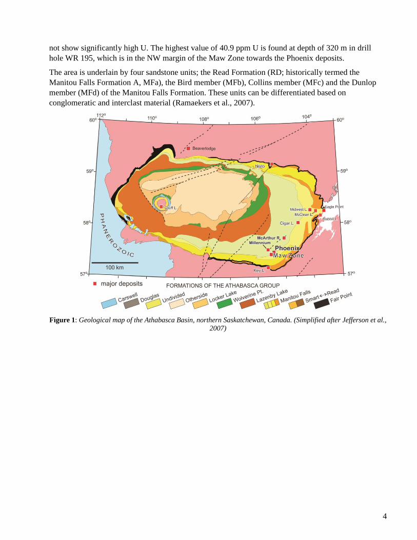
Geology of the Maw Zone

The Maw Zone, with a surface exposure of 300 x 200 m, is a breccia pipe from the unconformity to

the surface in the southeast part of Athabasca Basin (Figs. 1 and 2). The Maw Zone consists of highly

silicified, hematitized, dravitic tourmaline-rich rocks with high REE (up to 8.1 wt% as total oxides,

Agip Ltd, 1985). The Zone is ~ 4 km SW from the south end of deposit B of the Denison Mines’

Phoenix uranium deposits along the same NE-trending structure, but most rocks in the Maw Zone do

4

not show significantly high U. The highest value of 40.9 ppm U is found at depth of 320 m in drill

hole WR 195, which is in the NW margin of the Maw Zone towards the Phoenix deposits.

The area is underlain by four sandstone units; the Read Formation (RD; historically termed the

Manitou Falls Formation A, MFa), the Bird member (MFb), Collins member (MFc) and the Dunlop

member (MFd) of the Manitou Falls Formation. These units can be differentiated based on

conglomeratic and interclast material (Ramaekers et al., 2007).

Figure 1: Geological map of the Athabasca Basin, northern Saskatchewan, Canada. (Simplified after Jefferson et al.,

2007)

5

Figure. 2: Schematic vertical section showing the geology of the Maw Zone. (modified after Gamelin et al., 2010)

Application of PCA to the Maw Zone Geochemical Data

For the Maw Zone dataset all the samples are from four sandstones units (RD, MFb, MFc and MFd).

The geochemical analyses were determined at the Saskatchewan Research Council by the request of

Denison Mines using inductively coupled plasma optical emission spectrometry and inductively

coupled plasma mass spectrometry (ICP-MS) following a total digestion (An aliquot of pulp is

digested to dryness in a hot block digestion system using a mixture of ultra pure concentrated acids

HF:HNO3:HClO4. The residue is dissolved in 15 mL of 5% HNO3 and made to volume using de-

ionized water prior to analysis). Details on analysis method and the Quality Assurance/Quality Control

procedures followed are provided by Roscoe (2012).

The dataset contains 545 samples, each of which includes concentration data of 43 elements. After a

centered log-ratio transformation of the raw data, the elemental assemblages were evaluated using

simultaneous RQ-mode PCA. The analysis was carried out with the R statistical package

(R.Development Core Team, 2008) In this paper, 7 elements (Ag, Co, Mo, Sn, Ta, Tb, and W) with

many values were reported at less than or close to the detection limit. These elements provide very

limited information and were not retained. LREEs refers to light rare earth elements (La, Ce, Nd, Sm),

and HREEs heavy rare earth elements (Dy, Yb, Er, Gd).

The results of the RQ-PCA are shown in Tables 1 and 2, which list the eigenvalues, R-mode loadings

and the relative and actual contributions of the variables. Table 1 shows the results for the first seven

components only, which account for more than 69.3% of the variation in the data. Sums of the squares

of the loadings for PCs 1 to 7 represent the proportion of the total variability for each element captured

in the 7 PC model. The PC1-7 communalities of REEs, Y and U show high values, indicating that the

these seven components capture the variability of those elements. The relative contributions of Sr,

LREEs, Th, U, Ti, V, Y and HREEs account for most of the variation of the entire dataset (Table 3).

The screeplot displays the successive eigenvalues for all components (Figure 3).

6

Figure 3: Screeplot of Maw Zone, all sandstones dataset

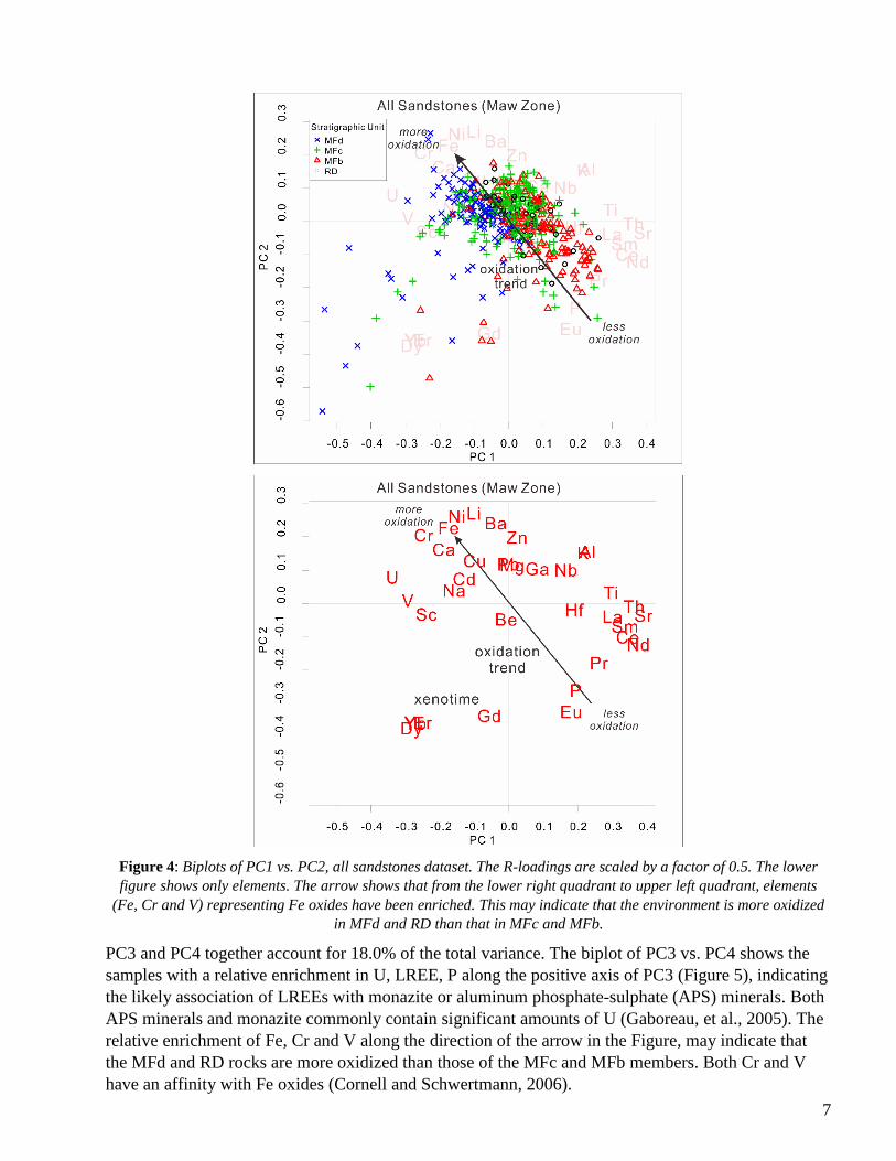
The biplot of PC1 vs. PC2 is shown in Figure 4. The scores of the observations are displayed as

symbols and the loadings of the elements are plotted. The symbols are associated with the four

lithologies associated with the samples. Examination of the actual contributions of PC1 (Table 4)

shows that Sr, LREEs, Th, U, Ti, V, Y and HREEs in that decreasing order, account for most of the

variation of this component. Note that a scaling factor of 0.5 was applied to the R-loadings in Figure 4.

PC1 and PC2 account for 36.3% of the total variability in the all sandstone dataset (Table 1). Relative

enrichment of HREEs and Y is observed along the negative PC2 axis in samples from the upper MFb,

MFc and MFd members of the Manitou Falls Formation. The plot shows the separation of HREEs and

LREEs, and the fractionation of Eu from the rest of REE. LREEs enrichment along PC1 and the

intermediate nature of P (between the HREEs & LREEs) suggest that samples contain high HREEs or

LREEs also contain high P. Therefore, the HREEs are likely hosted by xenotime and the LREEs by

monazite. Europium is commonly fractionated from the rest of the REEs because the valence of Eu is +2 or +3 in natural environments. Ca-rich plagioclase is the major host of Eu2+ and mafic igneous rocks

commonly contain high amounts of Eu. On the other hand, felsic rocks show low Eu concentrations.

The contents of Eu are very low in our samples, suggesting little interaction between hydrothermal

fluids and mafic rocks.

The diagram shows the enrichment of Fe in the upper left quadrant. Fe is most likely hosted by

hematite, which is abundant in all rock samples. Therefore, the enrichment of Fe is attributed to the

presence of an oxidized environment. Since the concentrations of Fe are relatively higher towards the

upper left, the sandstone samples plotted towards the direction are interpreted to be more oxidized.

Uranium concentrations are overall low (< 7.89 ppm), although the values for most samples are higher

than the average crustal concentration of 0.91 ppm (Taylor and McLennan, 1985). Uranium shows

positive correlations with Fe, V and Cr, suggesting that high contents of U are associated with

hematite, therefore, U was likely introduced by oxidizing fluids. The enrichment of Fe in upper left

quadrant also indicates that the environment was more oxidized in MFd and RD rocks than in the MFc

and MFb.

0 5 10 15 20 25 30 35

01

23

45

67

Maw Geochemistry - Total

Eigenvalue Number

Eig

envalu

e

7

Figure 4: Biplots of PC1 vs. PC2, all sandstones dataset. The R-loadings are scaled by a factor of 0.5. The lower

figure shows only elements. The arrow shows that from the lower right quadrant to upper left quadrant, elements

(Fe, Cr and V) representing Fe oxides have been enriched. This may indicate that the environment is more oxidized

in MFd and RD than that in MFc and MFb.

PC3 and PC4 together account for 18.0% of the total variance. The biplot of PC3 vs. PC4 shows the

samples with a relative enrichment in U, LREE, P along the positive axis of PC3 (Figure 5), indicating

the likely association of LREEs with monazite or aluminum phosphate-sulphate (APS) minerals. Both

APS minerals and monazite commonly contain significant amounts of U (Gaboreau, et al., 2005). The

relative enrichment of Fe, Cr and V along the direction of the arrow in the Figure, may indicate that

the MFd and RD rocks are more oxidized than those of the MFc and MFb members. Both Cr and V

have an affinity with Fe oxides (Cornell and Schwertmann, 2006).

8

An insight into elemental assemblages may be gained by observing the PCA results for individual rock

units. From the PC1-PC2 biplot for the RD data, U is associated with V and Cr and characterizes

samples with relative enrichment along the negative PC2 axis with Y and the REEs (Figure 6).

Phosphorus is weakly associated with the REEs, potentially indicating a change in the REE

mineralogy. Uraninite, monazite, xenotime and APS minerals are possible hosts of REEs in the RD

Formation. The relative enrichment of Fe, V and Cr in the lower left quadrant suggests that the U- and

REE-bearing minerals occur in oxidized sandstones.

Figure 5: Biplot of PC3 vs. PC4, all sandstones dataset. The R-loadings are scaled by a factor of 0.5. The lower

figure shows only elements. The arrow shows similar trend with Figure 3: Fe, Cr and V are enriched along the

arrow. The arrow also shows the enrichment trend of the LREEs.

9

Figure 6: Biplot of PC1 vs. PC2 for the RD dataset. The arrow shows that Fe, V and Cr have been enriched from the

upper right quadrant to the lower left quadrant. The host minerals of U and the REEs occur in an oxidized

environment, whereas elsewhere in the system a less oxidized environment predominates.

The PC1 v. PC2 biplot for MFb shows the samples with relative enrichment in LREEs-P-Sr along PC1

axis (Figure 7), indicating the possible occurrence of monazite and Sr-rich APS minerals. These

minerals are reported to contain significant Th at the Maw Zone, up to 3.5 and 2.3 wt.% ThO2

respectively (Pan et al., 2013). Uranium is grouped with elements that have an affinity to oxides, such

as Fe, V and Cr. The arrow shows the Fe, V and Cr enrichment trend, indicating that APS minerals

and monazite occur in a less oxidized environment.

The biplot of PC1 vs. PC2 for MFc shows that U is associated with Fe, Cr, V, and Cu (Figure 8).

Grouping of Sr-P-the LREEs and the HREEs-Y along the negative PC2 axis suggests the possible

presence of APS minerals, monazite and xenotime. The PC1 vs. PC2 biplot for MFd shows samples

with relative enrichment in Y-HREEs-P along the PC1 axis (Figure 9), which likely indicates the

occurrence of xenotime.

The 3D diagrams of drill holes and scores of PC1 and PC2 of total dataset (Figure 10) in the Maw

Zone show that Sr, Th, Y, the LREEs, Ti, V and U, contribute mostly to the variation of PC1, and the

HREEs, P, Y Li, Ni and Ba for PC2. Negative scores of PC1 and PC2 appear in the upper part of

sandstones (MFc and MFd). Since the HREEs and Y show strongly negative scores on PC2, this

reflects the occurrence of xenotime in the upper sandstone units.

10

Figure 7: Biplot of PC1 vs. PC2 for the MFb dataset. The arrow shows that Fe, V and Cr have been enriched along

this direction. This may indicate that Monazite and APS minerals occur in a less oxidized environment.

Figure 8: Biplot of PC1 vs PC2 for the MFc dataset. The arrow shows that Fe, V and Cr have been enriched along

this direction. Monazite and xenotime occur in a less oxidized environment.

11

Figure 9: Biplot of PC1 vs PC2 for the MFd dataset. The arrow shows that Fe, V and Cr have been enriched along

this direction. Monazite and xenotime occur in a less oxidized environment.

12

Figure 10: 3D Plot of PCA scores (all sandstone dataset) to depth

Summary

PCA is based on the estimation of the moments of data from which eigenvalues and eigenvectors are

extracted. It is useful in reducing the number of observed variables into a smaller number of artificial

variables that account for most of the variance in the given dataset. For the Maw Zone dataset (545

samples, each sample containing the concentrations of 36 elements), RQ-mode PCA appears to be

well suited for evaluating the elemental association and geological processes associated with the

geochemical dataset because it can display the relationships of the samples and elements at a same

scale.

The results of the principal component analysis applied to the geochemical data from the Maw Zone

reveals relative enrichment of groups of elements in different stratigraphic units;

1. The relative enrichment of HREEs-Y-P is observed in MFb, MFc and MFd, suggesting that

xenotime as the predominant host of the HREEs. The grouping of LREEs-Sr-Th-P in MFb

may reflect monazite and/or APS minerals.

2. The positive correlation between U and Fe and their loadings in the oxidized regions of the

biplots are consistent with overall low concentrations of U in the Maw Zone. Oxidizing fluids

transporting U were not reduced to precipitate significant amounts of U.

13

Acknowledgements

We thank Denison Mines Ltd., especially Lawson Forand, for providing the geochemical data and

approving the publication of this manuscript. A careful review by an anonymous reviewer improved

the clarity of the manuscript. The research project is funded by a grant to K.H. from Natural Resources

of Canada through the TGI-4 program. We thank an anonymous reviewer from the Geological Survey

of Canada for a critical review of the manuscript.

14

References

Agip Canada Ltd., 1985. Assessment File 74H06-NW-0080. Sask. Energy and Mines.

Aitchison, J., 1986. The Statistical Analysis of Compositional Data. Chapman and Hall: London. 436p.

Cornell, R.M. and Schwertmann, U., 2006. The Iron Oxides: Structure, Properties, Reactions, Occurrences and Uses.

Wiley. 703p.

Davis, J.C., 2002. Statistics and Data Analysis in Geology. 3rd editionn. John Wiley & Sons Inc. 656p.

Egozcue, J.J., Pawlowsky-Glahn V., Mateu-Figueraz G., and Barcel o-Vidal C., 2003. Isometric log-ratio

transformations for compositional data analysis. Math. Geol. 35:279-300.

Filzmoser, P., Hron, K., and Reimann, C., 2007 Principal component analysis for compositional data with outliers.

Special Issue: The 18th TIES Conference: Computational Environmetrics: Protection of Renewable Environment

and Human and Ecosystem Health. 20 (6): 621–632.

Gaboreau, S., Beaufort, D., Vieillard, P., Patrier, P., and Bruneton, P., 2005. Aluminum phosphate–sulfate minerals

associated with Proterozoic unconformity-type uranium deposits in the east Alligator River uranium field,

Northern Territories, Australia. The Canadian Mineralogist, 43(2): 813-827.

Gabriel, K.R., 1971. The biplot graphic display of matrices with application to principal component analysis,

Biometrika, 58 (3): 453-467.

Gamelin, C., Sorba, C., and Kerr, W., 2010. The discovery of the Phoenix Deposit: A new high-grade Athabasca

Basin unconformity-type uranium deposit, Saskatchewan, Canada: Saskatchewan Geol. Surv. Canada Open

House 2010. Abstract Volume 17.

Grunsky, E.C., 1986. Recognition of alteration in volcanic rocks using statistical analysis of lithogeochemical data;

Journal of Geochemical Exploration, 25: 157-183.

Grunsky, E.C., 2001. A program for computing RQ-mode principal components analysis for S-plus and R.

Computers & Geosciences, 27: 229–235.

Grunsky, E.C., Drew, L.J., and Sutphin, D.M., 2009. Process recognition in multi-element soil and stream-sediment

geochemical data. Applied Geochemistry, 24(8): 1602-1616.

Grunsky, E.C., 2010. The interpretation of geochemical survey data. Geochemistry-Exploration Environment

Analysis, 10(1): 27-74.

Hotelling, H., 1933. Analysis of a complex of statistical variables into principal components. Journal of Educational

Psychology, 24: 417-441, and 498-520.

Hron, K.,Templ, M., and Filzmoser, P, 2010. Imputation of missing values for compositional data using classical and

robust methods, Computational Statistics and Data Analysis, 54 (12): 3095-3107.

Jackson, J.E., 2003. A user’s guide to principal components. Wiley-Interscience, Hoboken, NJ. 575p.

Jefferson, C.W., Thomas, D.J., Gandhi, S.S., Ramaekers, P., Delaney, G., Brisbin, D., Cutts, C., Portella, P., and

Olson, R.A., 2007. Unconformity-associated uranium deposits of the Athabasca Basin, Saskatchewan and

Alberta. In: Jefferson, C.W., Delaney, G. (Eds.), EXTECH IV: Geology and Uranium EXploration TECHnology

of the Proterozoic Athabasca Basin, Saskatchewan and Alberta: Bulletin 588: Geological Survey of Canada (also

Special Publication 18: Saskatchewan Geological Society, pp. 23-68.

Jöreskog, K.G., Klovan, J.E., and Reyment, R.A., 1976. Geological Factor Analysis, Elsevier Scientific Publishing

Company, 178p.

Jolliffe, I.T., 1986. Principal Component Analysis. Encyclopedia of Statistics in Behavioral Science. John Wiley &

Sons, Ltd, 487p.

Jolliffe, I.T., 2002, Principal components analysis. 2nd edition. Springer, New York. 271p.

Klovan, J.E., and Imbrie, J., 1971. An algorithm and Fortran IV Program for large-scale Q–Mode Factor Analysis

and Calculation of Factor Scores. Mathematical Geology. 3:61-67.

Neff, H. 1994. RQ-mode principal components analysis of ceramic compositional data. Archaeometry 36:115-130.

Pan, Y., Yeo, G., Rogers, B., Austman, C., and Hu, B., 2013, Application of radiation-induced defects in quartz to

exploration for uranium deposits: a case study of the Maw Zone, Athabasca Basin, Saskatchewan. Explor. Mining

Geol. v. 21, p. 115-128.

Pearson, K., 1901. On lines and planes of closest fit to systems of points in space. Philosophical Magazine 2 (11):

559–572.

15

R Development Core Team, 2008. R: A language and environment for statistical computing. R Foundation for

Statistical Computing, Vienna, Austria. ISBN 3-900051-07-0, URL: http://www.R-project.org

Ramaekers, P., Jefferson, C.W., Yeo, G.M., Collier, B., Long, D.G.F., Drever, G., McHardy, S., Jiricka, D., Cutts,

C., Wheatley, K., Catuneanu, O., Bernier, S., Kupsch, B., and Post, R.T., 2007, Revised geological map and

stratigraphy of the Athabasca Group, Saskatchewan and Alberta. In EXTECH IV: Geology and Uranium

EXploration TECHnology of the Proterozoic Athabasca Basin, Saskatchewan and Alberta, edited by C.W.

Jefferson and G. Delaney, Geological Survey of Canada Bulletin 588, 155-191 (also Saskatchewan Geological

Society Special Publication 18; Geological Association of Canada, Mineral Deposits Division, Special

Publication 4).

Reyment, R.A. and Jöreskog, K.G., 1996. Applied Factor Analysis in the Natural Sciences. Cambridge University

Press. 371p.

Roscoe, W.E., 2012. Technical report on a mineral resource estimate update for the Phoenix uranium deposits,

Wheeler river project, Eastern Athabasca basin, Northern Saskatchewan, Canada. NI 43-101 Report prepared for

Denison Mines Corp.

Taylor, S.R. and McClennan, S.M., 1985. The Continental Crust: Its Composition and Evolution. Blackwell, Oxford.

312p.

Zhou D., Chang T., and Davis J.C., 1983. Dual extraction of R-mode and Q-mode factor solutions. Mathematical

Geology, 15: 581–606.

16

Table 1. Eigenvalues of principal components of Maw Zone data. Analysis carried out on log-centred data.

Eigenvalue

PC1 PC2 PC3 PC4 PC5 PC6 PC7

λ 7.59 5.42 3.73 2.73 2.12 1.90 1.39

λ% 21.13% 15.08% 10.38% 7.60% 5.91% 5.29% 3.87%

Σ 21.13% 36.21% 46.59% 54.19% 60.10% 65.39% 69.26%

17

Table 2. Loading values of elements for each principal components 1 to 7.

R-Loading values

PC1 PC2 PC3 PC4 PC5 PC6 PC7 Sum of the square of the

loadings PC1 to PC7

U -0.67 0.16 0.41 0.06 -0.03 0.11 -0.07 0.67

Cu -0.20 0.26 0.10 -0.29 0.37 0.27 0.21 0.47

La 0.60 -0.07 0.48 -0.12 -0.06 -0.08 0.25 0.68

Fe -0.31 0.48 0.53 0.13 0.00 0.14 0.11 0.66

Ni -0.28 0.48 0.06 0.02 0.39 0.19 0.31 0.60

P 0.39 -0.51 0.20 0.06 -0.34 -0.14 0.18 0.62

Pb -0.01 0.24 0.20 0.35 -0.32 -0.08 -0.15 0.35

V -0.58 0.02 -0.23 -0.20 -0.10 -0.18 -0.25 0.53

Y -0.57 -0.71 -0.11 0.06 0.10 0.01 -0.14 0.88

Zn 0.04 0.40 0.07 0.39 0.45 -0.06 0.16 0.55

Al 0.45 0.32 -0.57 -0.12 -0.04 -0.42 0.13 0.84

Ba -0.08 0.49 0.26 0.26 -0.53 -0.22 -0.11 0.71

Be -0.02 -0.09 0.01 -0.74 -0.27 0.01 0.06 0.63

Ca -0.38 0.33 0.33 -0.09 -0.46 -0.01 0.05 0.59

Cd -0.26 0.15 0.04 -0.24 0.28 0.11 -0.34 0.36

Ce 0.68 -0.20 0.52 -0.20 0.21 -0.07 -0.14 0.89

Cr -0.50 0.42 0.56 0.04 0.17 0.21 0.08 0.81

Dy -0.57 -0.75 -0.10 0.07 -0.10 0.01 0.12 0.93

Er -0.50 -0.71 -0.16 0.21 0.01 0.07 0.11 0.84

Eu 0.36 -0.64 0.02 -0.01 0.21 -0.06 -0.01 0.59

Ga 0.16 0.21 -0.52 -0.43 0.16 -0.20 -0.28 0.67

Gd -0.12 -0.67 0.21 0.28 0.14 -0.17 0.00 0.63

Hf 0.38 -0.03 -0.30 -0.02 -0.04 0.63 -0.29 0.71

K 0.43 0.31 -0.43 0.44 0.07 -0.41 0.03 0.84

Li -0.21 0.55 -0.18 0.16 0.09 -0.30 -0.27 0.58

Mg 0.02 0.22 -0.47 -0.57 0.12 0.01 0.29 0.70

Na -0.32 0.09 0.15 -0.68 -0.34 0.02 0.12 0.73

Nb 0.33 0.21 -0.20 0.26 -0.14 0.51 -0.33 0.64

Nd 0.75 -0.24 0.41 -0.13 0.28 -0.07 -0.11 0.89

Pr 0.52 -0.35 0.32 -0.27 0.01 -0.08 -0.30 0.66

Sc -0.48 -0.06 0.31 -0.14 -0.14 -0.09 -0.40 0.54

Sm 0.67 -0.13 0.46 -0.08 0.28 -0.02 -0.17 0.78

Sr 0.78 -0.06 0.24 0.04 -0.32 -0.08 0.21 0.82

Th 0.72 -0.01 -0.15 0.15 -0.20 0.38 0.09 0.76

Ti 0.59 0.08 -0.39 0.10 -0.28 0.47 0.03 0.82

Yb -0.55 -0.71 -0.24 0.13 -0.03 0.11 0.13 0.91

18

Table 3. Relative contribution of elements for each principal components

Relative Contributions

PC1 PC2 PC3 PC4 PC5 PC6 PC7

U 45.62 2.66 17.03 0.42 0.07 1.17 0.49

Cu 4.08 6.89 1.00 8.65 14.09 7.57 4.57

La 35.94 0.51 23.08 1.42 0.34 0.69 6.21

Fe 9.81 22.91 28.59 1.74 0.00 2.07 1.30

Ni 7.92 22.94 0.32 0.03 15.41 3.58 9.44

P 14.94 26.28 3.85 0.33 11.77 1.83 3.17

Pb 0.01 5.85 3.96 12.35 10.26 0.71 2.24

V 34.21 0.06 5.11 3.83 0.92 3.40 6.05

Y 32.92 50.36 1.25 0.32 1.08 0.02 2.07

Zn 0.18 16.20 0.53 15.23 20.22 0.35 2.56

Al 20.60 10.05 32.07 1.49 0.18 17.69 1.68

Ba 0.65 23.84 6.68 6.53 27.89 4.75 1.13

Be 0.04 0.79 0.01 54.28 7.38 0.02 0.39

Ca 14.40 11.05 10.93 0.86 21.57 0.00 0.26

Cd 6.82 2.33 0.16 5.77 7.99 1.17 11.80

Ce 46.73 3.83 27.51 3.89 4.42 0.45 1.87

Cr 24.56 17.38 31.11 0.20 2.90 4.58 0.72

Dy 32.47 56.79 1.09 0.49 0.92 0.02 1.49

Er 25.18 50.36 2.62 4.30 0.00 0.51 1.23

Eu 12.81 41.27 0.03 0.00 4.61 0.40 0.01

Ga 2.64 4.57 26.93 18.10 2.59 4.16 8.04

Gd 1.39 44.78 4.26 7.90 1.96 2.77 0.00

Hf 14.27 0.10 9.31 0.03 0.19 39.29 8.26

K 18.54 9.59 18.75 19.61 0.46 16.93 0.10

Li 4.23 29.89 3.40 2.65 0.86 9.30 7.35

Mg 0.03 5.02 21.77 32.75 1.43 0.02 8.69

Na 10.43 0.74 2.24 46.72 11.32 0.06 1.48

Nb 10.72 4.33 4.12 6.90 1.88 25.85 10.65

Nd 55.70 5.74 16.60 1.72 7.87 0.54 1.32

Pr 27.10 12.31 10.00 7.44 0.01 0.59 8.78

Sc 23.32 0.35 9.64 1.94 1.99 0.79 15.94

Sm 44.61 1.66 20.75 0.64 8.07 0.03 2.81

Sr 60.18 0.42 5.72 0.19 10.28 0.57 4.56

Th 52.48 0.01 2.22 2.25 3.99 14.82 0.83

Ti 35.05 0.59 15.28 0.99 7.58 22.59 0.08

Yb 29.99 50.56 5.80 1.65 0.09 1.15 1.60

19

Table 4. Actual contribution of elements for each principal components

Actual Contributions

PC1 PC2 PC3 PC4 PC5 PC6 PC7

U 6.00 0.49 4.56 0.15 0.03 0.61 0.35

Cu 0.54 1.27 0.27 3.16 6.63 3.97 3.28

La 4.73 0.09 6.18 0.52 0.16 0.36 4.46

Fe 1.29 4.22 7.65 0.64 0.00 1.08 0.93

Ni 1.04 4.23 0.09 0.01 7.25 1.88 6.78

P 1.96 4.84 1.03 0.12 5.53 0.96 2.28

Pb 0.00 1.08 1.06 4.51 4.82 0.37 1.61

V 4.50 0.01 1.37 1.40 0.43 1.79 4.35

Y 4.33 9.27 0.33 0.12 0.51 0.01 1.49

Zn 0.02 2.98 0.14 5.57 9.51 0.18 1.84

Al 2.71 1.85 8.58 0.54 0.09 9.29 1.21

Ba 0.09 4.39 1.79 2.39 13.12 2.50 0.81

Be 0.01 0.15 0.00 19.84 3.47 0.01 0.28

Ca 1.89 2.04 2.92 0.31 10.15 0.00 0.19

Cd 0.90 0.43 0.04 2.11 3.76 0.62 8.48

Ce 6.14 0.71 7.36 1.42 2.08 0.23 1.34

Cr 3.23 3.20 8.33 0.07 1.37 2.41 0.52

Dy 4.27 10.46 0.29 0.18 0.43 0.01 1.07

Er 3.31 9.27 0.70 1.57 0.00 0.27 0.89

Eu 1.68 7.60 0.01 0.00 2.17 0.21 0.01

Ga 0.35 0.84 7.21 6.62 1.22 2.18 5.78

Gd 0.18 8.25 1.14 2.89 0.92 1.45 0.00

Hf 1.88 0.02 2.49 0.01 0.09 20.63 5.94

K 2.44 1.77 5.02 7.16 0.22 8.89 0.07

Li 0.56 5.50 0.91 0.97 0.41 4.88 5.28

Mg 0.00 0.93 5.82 11.97 0.67 0.01 6.24

Na 1.37 0.14 0.60 17.07 5.32 0.03 1.06

Nb 1.41 0.80 1.10 2.52 0.88 13.58 7.65

Nd 7.32 1.06 4.44 0.63 3.70 0.28 0.95

Pr 3.56 2.27 2.68 2.72 0.00 0.31 6.31

Sc 3.07 0.06 2.58 0.71 0.94 0.41 11.45

Sm 5.87 0.31 5.55 0.24 3.79 0.01 2.02

Sr 7.91 0.08 1.53 0.07 4.84 0.30 3.28

Th 6.90 0.00 0.59 0.82 1.88 7.78 0.60

Ti 4.61 0.11 4.09 0.36 3.56 11.86 0.06

Yb 3.94 9.31 1.55 0.60 0.04 0.60 1.15

20

Appendix. The Closure Problem

Aitchison (1986) and Filzmoser (2007) stated that compositional data are inherently closed data with

positive values that sum up to a constant, usually chosen as 1(100%). The inter-variable relationship is

not the real relationship, but a forced one. A good example from Filzmoser (2007) is that supposing a

rock sample was analyzed and the result showed that SiO2 was a big proportion, 70%, therefore the

concentration of the remaining elements determined automatically account for at most 30%. Any

increase in values of SiO2 automatically leads to decreases in values of the other elements. This

problem may result individual variables do not vary independently (See FigureA-1 for another

artificial example). However, the closure problem does not disappear automatically even some of the

variables are removed from the original dataset because although the values do not sum to a unit value,

they still sum to the unit value minus the omitted variables (Aitchison, 1986).

Statistical tools may produce uninterpretable results if they are directly applied to raw data without

log-ratio transformations Three kinds of log-ratio transformations are widely used - the additive log-

ratio and the centered log-ratio transformation (Aitchison, 1986) and the isometric log-ratio

transformation (Egozcue et al., 2003). The application of a centred log-ratio transformation will

provide more reliable and statistically sound results. The isometric log-ratio (Egozcue et al. 2003)

method may be used for data sets where balances between the elements are constructed and provides

orthonormal basis in the compositional data space.

Fig A-1. The incorrect biplot of PC1 vs PC2, MFb dataset. The PCA results have a data closure problem and show incorrect and uninterpretable elemental associations: HREE+Y dominates and other elements are crowded.

However, after eliminating data closure effects by applying centered log-ratio transformation, the correct plot

diagram (Figure 7) show interpretable elemental association: U is correlated with Ni, Cr, Fe,. etc, and REEs are correlated with P.

In this paper we solve the data closure problem by applying a centred log-ratio transformation which

provides a symmetrical treatment of all parts of a composition as described by Aitchison, (1986)

The log-centered-ratio transformation is a transformation from 𝒮𝐷 to ℝ𝐷, where

21

𝒮𝐷 = {𝑥 = (𝑥1, … , 𝑥𝐷)′, 𝑥𝑖 > 0, ∑ 𝑥𝑖 = 1}

𝐷

𝑖=1

Where the prime stands for transpose and the simplex sample space is a 𝐷 − 1 dimensional subset of

ℝ𝐷.

and the result for an observation 𝒙 ∈ 𝒮𝐷 are the transformed data 𝒚 ∈ ℝ𝐷 with

𝒚 = (𝑦1, … , 𝑦𝐷)′ = (log𝑥1

√∏ 𝑥𝑖𝐷𝑖=1

𝐷, … , log

𝑥𝐷

√∏ 𝑥𝑖𝐷𝑖=1

𝐷)

′

,

or written in matrix notation:

y = 𝑭 log(𝒙),

where

𝑭 = 𝑰𝐷 −1

𝐷𝑱𝐷, with 𝑰𝐷 = (

1 0 ⋱ 0 1

), 𝑱𝐷 = (1 ⋯ 0⋮ ⋱ ⋮0 ⋯ 1

)

The matrices F, 𝑰𝐷, and 𝑱𝐷 are all of dimension D×D. The centered log-ratio transformation treats all

components symmetrically by dividing by the geometric mean. Thus it is possible to use the original

variable names for the interpretation of statistical results based on centered log-ratio transformed data.