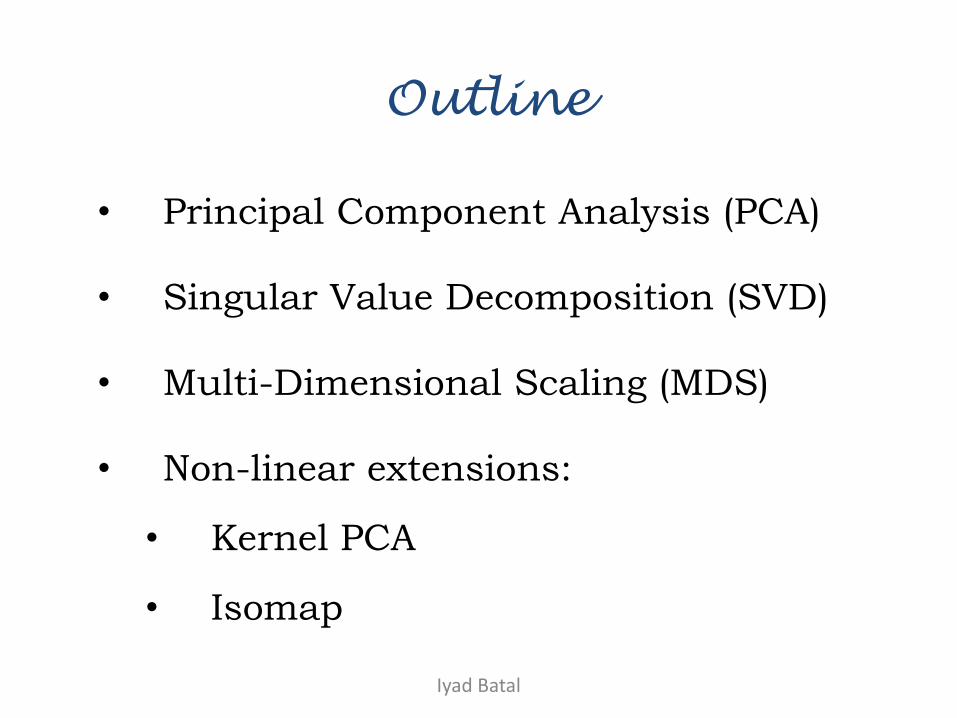
Outline

• Principal Component Analysis (PCA)

• Singular Value Decomposition (SVD)

• Multi-Dimensional Scaling (MDS)

• Non-linear extensions:

• Kernel PCA

• Isomap

Iyad Batal

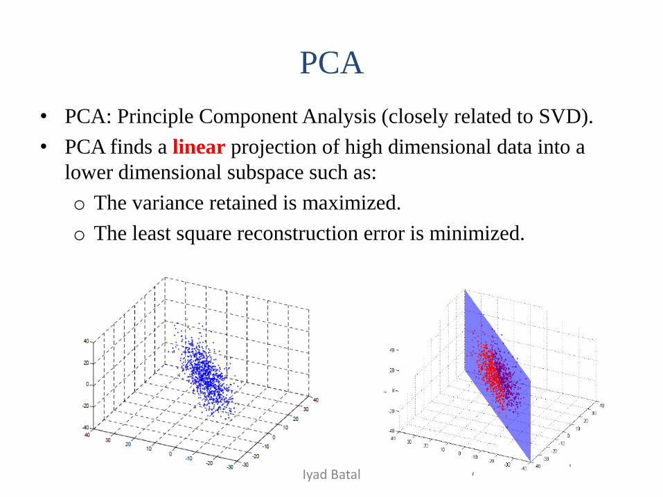
PCA

• PCA: Principle Component Analysis (closely related to SVD).

• PCA finds a linear projection of high dimensional data into a

lower dimensional subspace such as:

o The variance retained is maximized.

o The least square reconstruction error is minimized.

Iyad Batal

Some PCA/SVD applications

LSI: Latent Semantic Indexing.

Kleinberg/Hits algorithm (compute hubs and authority scores

for nodes).

Google/PageRank algorithm (random walk with restart).

Image compression (eigen faces)

Data visualization (by projecting the data on 2D).

Iyad Batal

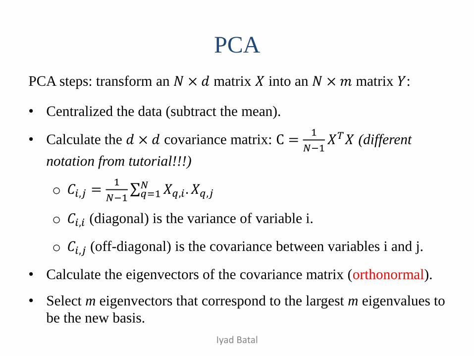
PCA

PCA steps: transform an 𝑁 × 𝑑 matrix 𝑋 into an 𝑁 × 𝑚 matrix 𝑌:

• Centralized the data (subtract the mean).

• Calculate the 𝑑 × 𝑑 covariance matrix: C =1

𝑁−1𝑋𝑇𝑋 (different

notation from tutorial!!!)

o 𝐶𝑖,𝑗 =1

𝑁−1 𝑋𝑞,𝑖 . 𝑋𝑞,𝑗

𝑁𝑞=1

o 𝐶𝑖,𝑖 (diagonal) is the variance of variable i.

o 𝐶𝑖,𝑗 (off-diagonal) is the covariance between variables i and j.

• Calculate the eigenvectors of the covariance matrix (orthonormal).

• Select m eigenvectors that correspond to the largest m eigenvalues to

be the new basis.

Iyad Batal

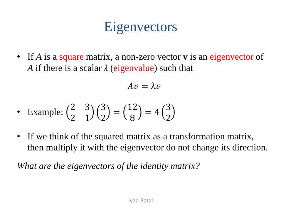
Eigenvectors

• If A is a square matrix, a non-zero vector v is an eigenvector of

A if there is a scalar λ (eigenvalue) such that

𝐴𝑣 = λ𝑣

• Example: 2 32 1

32

=128

= 432

• If we think of the squared matrix as a transformation matrix,

then multiply it with the eigenvector do not change its direction.

What are the eigenvectors of the identity matrix?

Iyad Batal

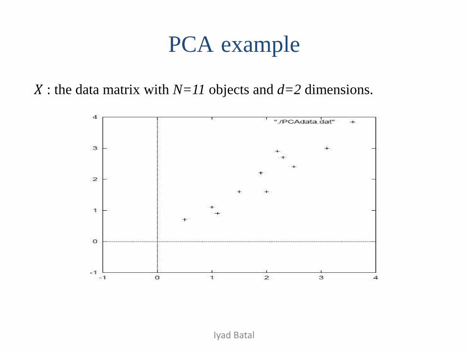
𝑋 : the data matrix with N=11 objects and d=2 dimensions.

Iyad Batal

PCA example

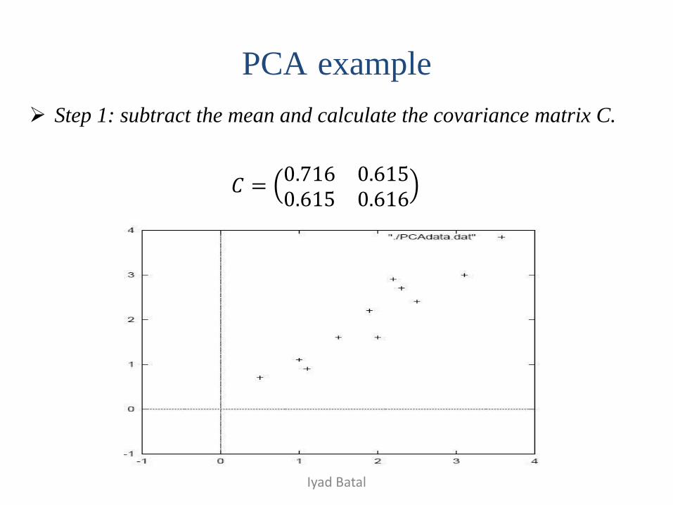
Step 1: subtract the mean and calculate the covariance matrix C.

𝐶 =0.716 0.6150.615 0.616

Iyad Batal

PCA example

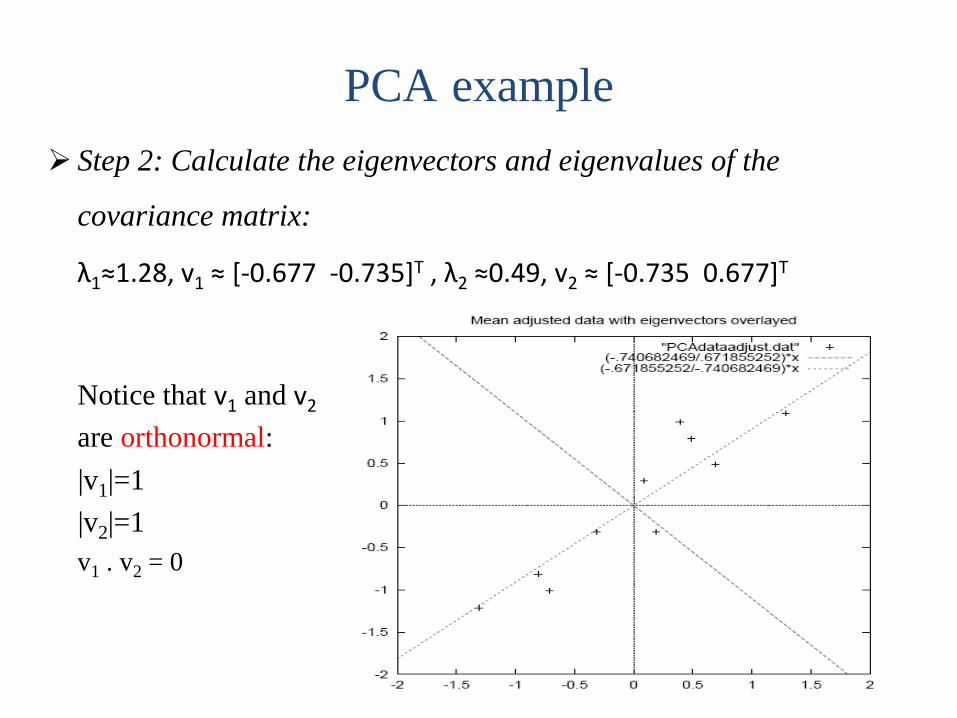
Step 2: Calculate the eigenvectors and eigenvalues of the

covariance matrix:

λ1≈1.28, v1 ≈ [-0.677 -0.735]T , λ2 ≈0.49, v2 ≈ [-0.735 0.677]T

Notice that v1 and v2

are orthonormal:

|v1|=1

|v2|=1

v1 . v2 = 0

Iyad Batal

PCA example

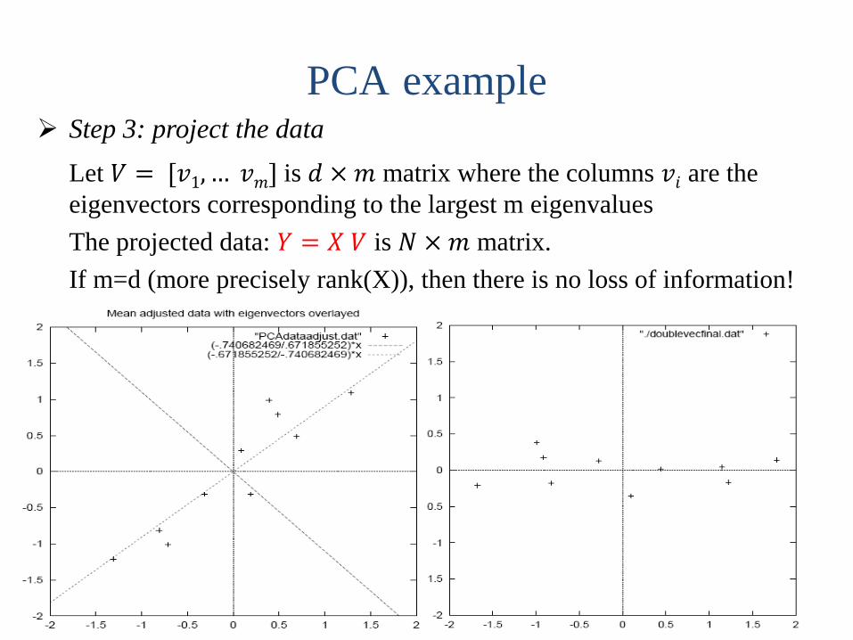
Step 3: project the data

Let 𝑉 = [𝑣1, … 𝑣𝑚] is 𝑑 × 𝑚 matrix where the columns 𝑣𝑖 are the

eigenvectors corresponding to the largest m eigenvalues

The projected data: 𝑌 = 𝑋 𝑉 is 𝑁 × 𝑚 matrix.

If m=d (more precisely rank(X)), then there is no loss of information!

Iyad Batal

PCA example

Step 3: project the data

λ1≈1.28, v1 ≈ [-0.677 -0.735]T , λ2 ≈0.49, v2 ≈ [-0.735 0.677]T

The eigenvector with the highest eigenvalue is the principle

component of the data.

if we are allowed to pick only one dimension, the principle

component is the best direction (retain the maximum variance).

Our PC is v1 ≈ [-0.677 -0.735]T

Iyad Batal

PCA example

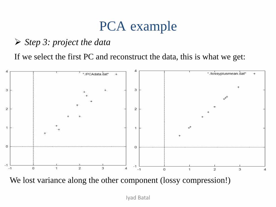
Step 3: project the data

If we select the first PC and reconstruct the data, this is what we get:

Iyad Batal

We lost variance along the other component (lossy compression!)

PCA example

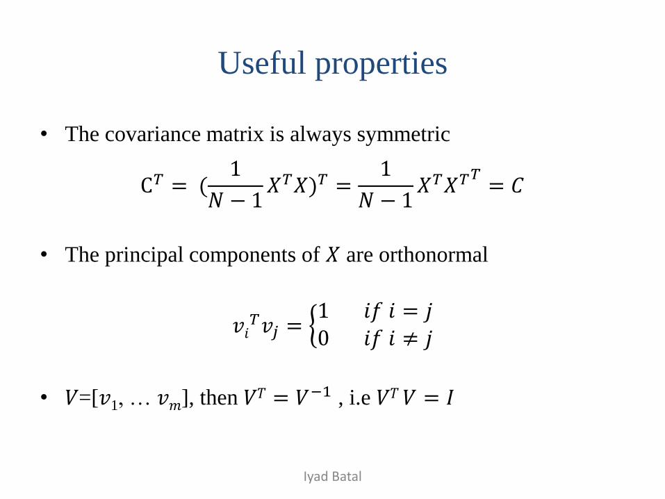
Useful properties

• The covariance matrix is always symmetric

C𝑇 = (1

𝑁 − 1𝑋𝑇𝑋)𝑇 =

1

𝑁 − 1𝑋𝑇𝑋𝑇𝑇

= 𝐶

• The principal components of 𝑋 are orthonormal

𝑣𝑖𝑇𝑣𝑗 =

1 𝑖𝑓 𝑖 = 𝑗0 𝑖𝑓 𝑖 ≠ 𝑗

• 𝑉=[𝑣1, … 𝑣𝑚], then 𝑉𝑇 = 𝑉−1 , i.e 𝑉𝑇 𝑉 = 𝐼

Iyad Batal

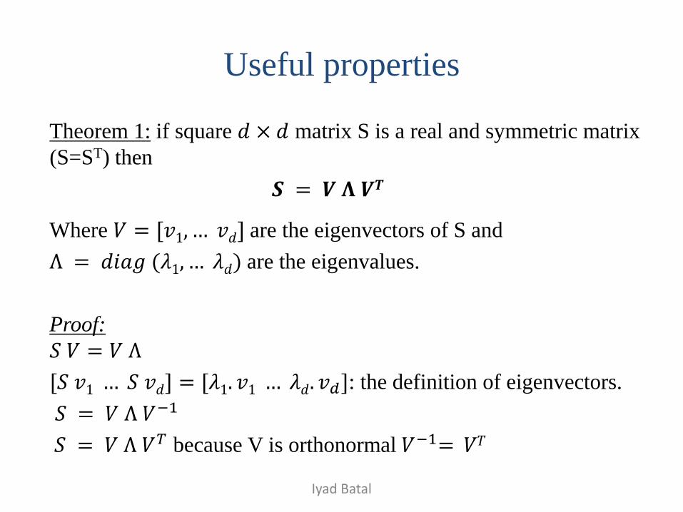
Useful properties

Theorem 1: if square 𝑑 × 𝑑 matrix S is a real and symmetric matrix

(S=ST) then

𝑺 = 𝑽 𝚲 𝑽𝑻

Where 𝑉 = [𝑣1, … 𝑣𝑑] are the eigenvectors of S and

Λ = 𝑑𝑖𝑎𝑔 (𝜆1, … 𝜆𝑑) are the eigenvalues.

Proof:

𝑆 𝑉 = 𝑉 Λ

[𝑆 𝑣1 … 𝑆 𝑣𝑑] = [𝜆1. 𝑣1 … 𝜆𝑑. 𝑣𝑑]: the definition of eigenvectors.

𝑆 = 𝑉 Λ 𝑉−1

𝑆 = 𝑉 Λ 𝑉𝑇 because V is orthonormal 𝑉−1= 𝑉𝑇

Iyad Batal

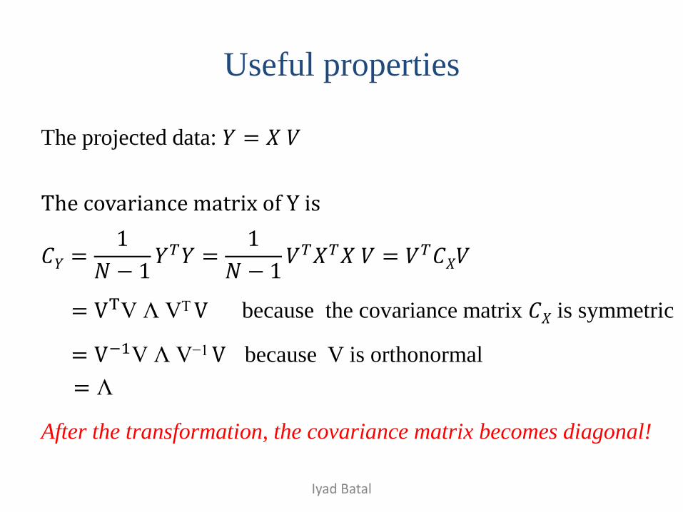
Useful properties

The projected data: 𝑌 = 𝑋 𝑉

The covariance matrix of Y is

𝐶𝑌 =1

𝑁 − 1𝑌𝑇𝑌 =

1

𝑁 − 1𝑉𝑇𝑋𝑇𝑋 𝑉 = 𝑉𝑇𝐶𝑋𝑉

= VTV Λ VT V because the covariance matrix 𝐶𝑋 is symmetric

= V−1V Λ V−1 V because V is orthonormal

= Λ

After the transformation, the covariance matrix becomes diagonal!

Iyad Batal

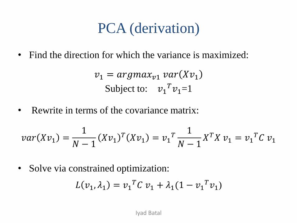
PCA (derivation)

• Find the direction for which the variance is maximized:

𝑣1 = 𝑎𝑟𝑔𝑚𝑎𝑥𝑣1 𝑣𝑎𝑟 𝑋𝑣1

Subject to: 𝑣1𝑇𝑣1=1

• Rewrite in terms of the covariance matrix:

𝑣𝑎𝑟 𝑋𝑣1 =1

𝑁 − 1𝑋𝑣1

𝑇 𝑋𝑣1 = 𝑣1𝑇

1

𝑁 − 1𝑋𝑇𝑋 𝑣1 = 𝑣1

𝑇𝐶 𝑣1

• Solve via constrained optimization:

𝐿 𝑣1, 𝜆1 = 𝑣1𝑇𝐶 𝑣1 + 𝜆1(1 − 𝑣1

𝑇𝑣1)

Iyad Batal

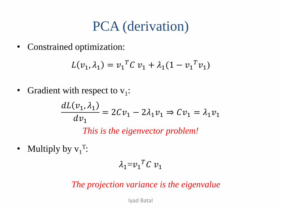
PCA (derivation)

• Constrained optimization:

𝐿 𝑣1, 𝜆1 = 𝑣1𝑇𝐶 𝑣1 + 𝜆1(1 − 𝑣1

𝑇𝑣1)

• Gradient with respect to v1:

𝑑𝐿 𝑣1, 𝜆1

𝑑𝑣1= 2𝐶𝑣1 − 2𝜆1𝑣1 ⇒ 𝐶𝑣1 = 𝜆1𝑣1

This is the eigenvector problem!

• Multiply by v1T:

𝜆1=𝑣1𝑇𝐶 𝑣1

The projection variance is the eigenvalue

Iyad Batal

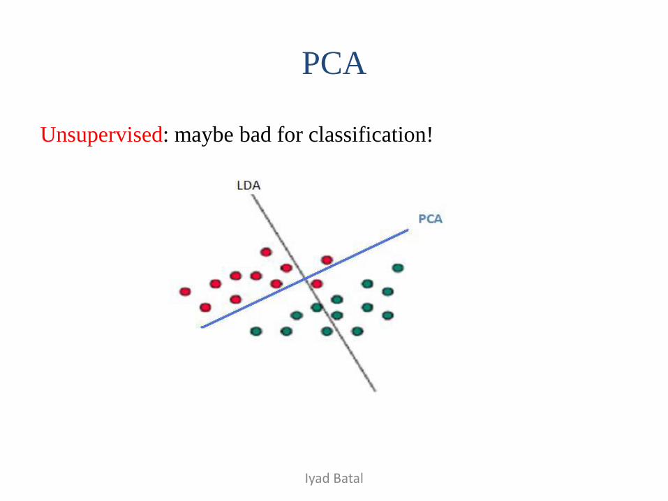
PCA

Unsupervised: maybe bad for classification!

Iyad Batal

Outline

• Principal Component Analysis (PCA)

• Singular Value Decomposition (SVD)

• Multi-Dimensional Scaling (MDS)

• Non-linear extensions:

• Kernel PCA

• Isomap

Iyad Batal

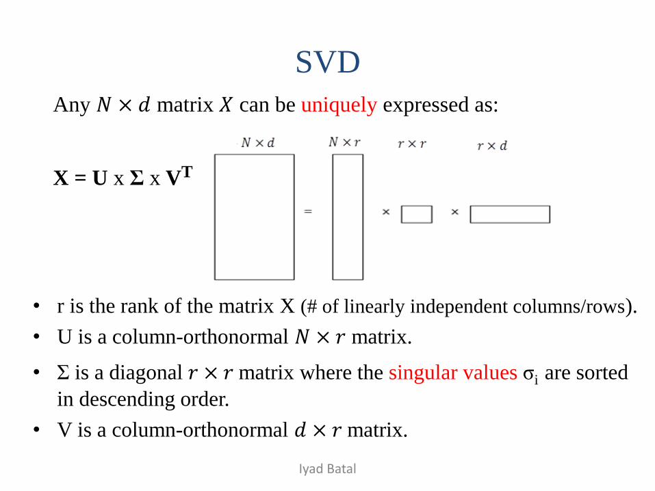
SVD

Any 𝑁 × 𝑑 matrix 𝑋 can be uniquely expressed as:

X = U x Σ x VT

• r is the rank of the matrix X (# of linearly independent columns/rows).

• U is a column-orthonormal 𝑁 × 𝑟 matrix.

• Σ is a diagonal 𝑟 × 𝑟 matrix where the singular values σi are sorted

in descending order.

• V is a column-orthonormal 𝑑 × 𝑟 matrix.

Iyad Batal

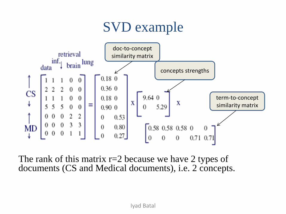
SVD example

The rank of this matrix r=2 because we have 2 types of documents (CS and Medical documents), i.e. 2 concepts.

Iyad Batal

doc-to-concept similarity matrix

concepts strengths

term-to-concept similarity matrix

doc-to-concept similarity matrix

concepts strengths

term-to-concept similarity matrix

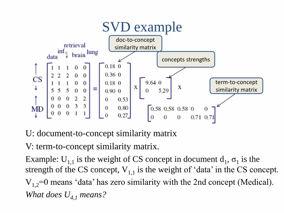
U: document-to-concept similarity matrix

V: term-to-concept similarity matrix.

Example: U1,1 is the weight of CS concept in document d1, σ1 is the

strength of the CS concept, V1,1 is the weight of ‘data’ in the CS concept.

V1,2=0 means ‘data’ has zero similarity with the 2nd concept (Medical).

What does U4,1 means?

SVD example

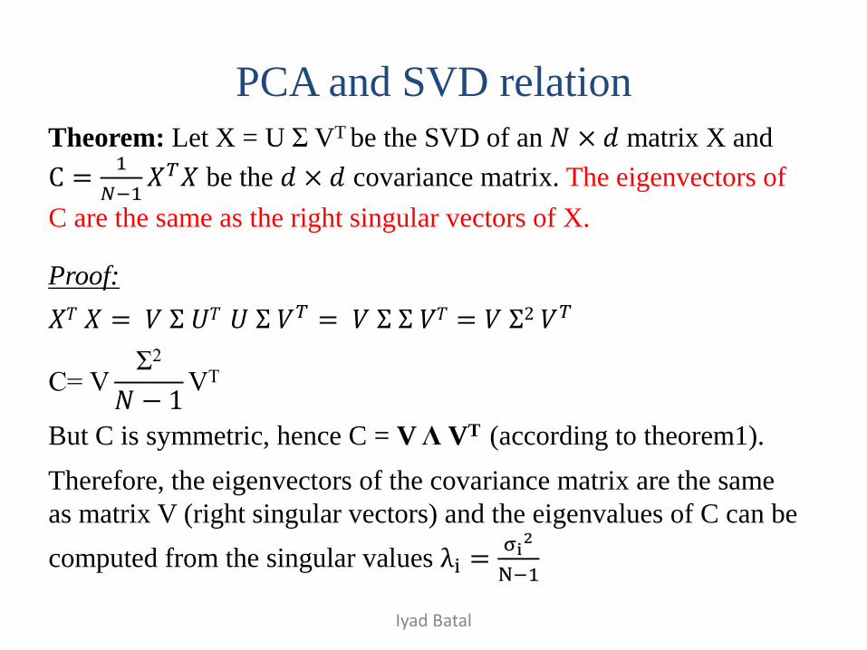
PCA and SVD relation

Theorem: Let X = U Σ VT be the SVD of an 𝑁 × 𝑑 matrix X and

C =1

𝑁−1𝑋𝑇𝑋 be the 𝑑 × 𝑑 covariance matrix. The eigenvectors of

C are the same as the right singular vectors of X.

Proof:

𝑋𝑇 𝑋 = 𝑉 Σ 𝑈𝑇 𝑈 Σ 𝑉𝑇 = 𝑉 Σ Σ 𝑉𝑇 = 𝑉 Σ2 𝑉𝑇

C= VΣ2

𝑁 − 1VT

But C is symmetric, hence C = V Λ VT (according to theorem1).

Therefore, the eigenvectors of the covariance matrix are the same

as matrix V (right singular vectors) and the eigenvalues of C can be

computed from the singular values λi =σi

2

N−1

Iyad Batal

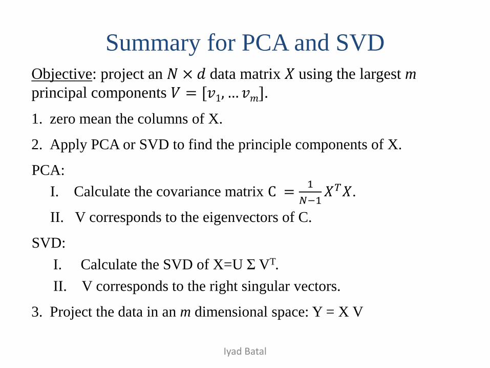
Summary for PCA and SVD

Objective: project an 𝑁 × 𝑑 data matrix 𝑋 using the largest m

principal components 𝑉 = [𝑣1, … 𝑣𝑚].

1. zero mean the columns of X.

2. Apply PCA or SVD to find the principle components of X.

PCA:

I. Calculate the covariance matrix C =1

𝑁−1𝑋𝑇𝑋.

II. V corresponds to the eigenvectors of C.

SVD:

I. Calculate the SVD of X=U Σ VT.

II. V corresponds to the right singular vectors.

3. Project the data in an m dimensional space: Y = X V

Iyad Batal

Outline

• Principal Component Analysis (PCA)

• Singular Value Decomposition (SVD)

• Multi-Dimensional Scaling (MDS)

• Non-linear extensions:

• Kernel PCA

• Isomap

Iyad Batal

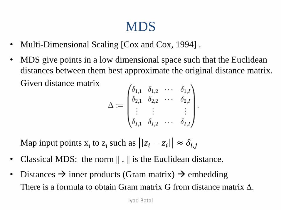
MDS

• Multi-Dimensional Scaling [Cox and Cox, 1994] .

• MDS give points in a low dimensional space such that the Euclidean

distances between them best approximate the original distance matrix.

Given distance matrix

Map input points xi to zi such as 𝑧𝑖 − 𝑧𝑖 ≈ 𝛿𝑖,𝑗

• Classical MDS: the norm || . || is the Euclidean distance.

• Distances inner products (Gram matrix) embedding

There is a formula to obtain Gram matrix G from distance matrix Δ.

Iyad Batal

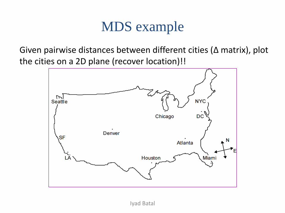
MDS example

Given pairwise distances between different cities (Δ matrix), plot the cities on a 2D plane (recover location)!!

Iyad Batal

PCA and MDS relation

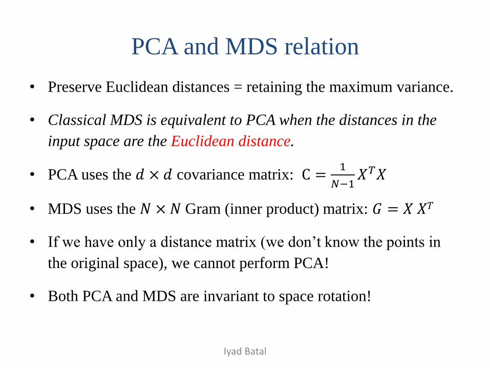
• Preserve Euclidean distances = retaining the maximum variance.

• Classical MDS is equivalent to PCA when the distances in the

input space are the Euclidean distance.

• PCA uses the 𝑑 × 𝑑 covariance matrix: C =1

𝑁−1𝑋𝑇𝑋

• MDS uses the 𝑁 × 𝑁 Gram (inner product) matrix: 𝐺 = 𝑋 𝑋𝑇

• If we have only a distance matrix (we don’t know the points in

the original space), we cannot perform PCA!

• Both PCA and MDS are invariant to space rotation!

Iyad Batal

Kernel PCA

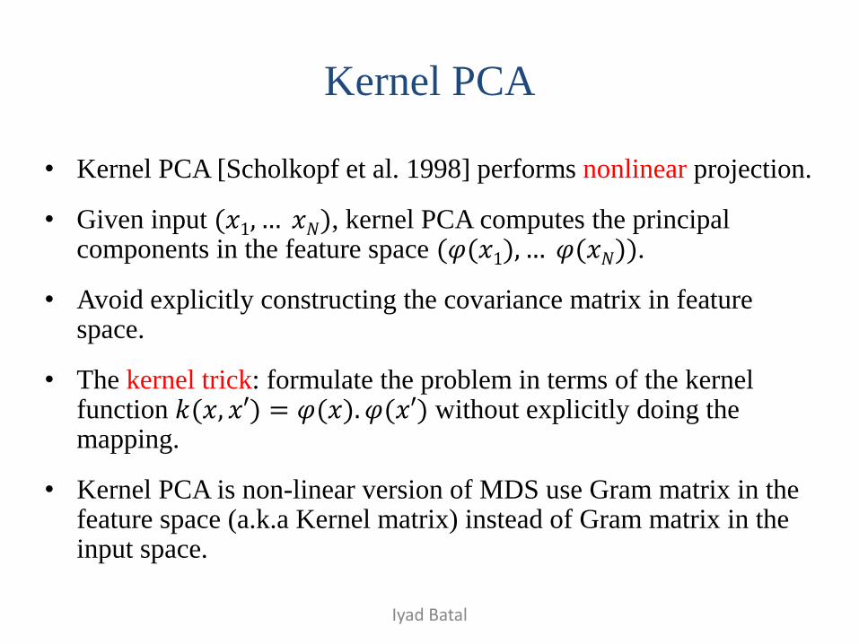
• Kernel PCA [Scholkopf et al. 1998] performs nonlinear projection.

• Given input (𝑥1, … 𝑥𝑁), kernel PCA computes the principal components in the feature space (𝜑(𝑥1), … 𝜑(𝑥𝑁)).

• Avoid explicitly constructing the covariance matrix in feature space.

• The kernel trick: formulate the problem in terms of the kernel function 𝑘(𝑥, 𝑥′) = 𝜑(𝑥). 𝜑(𝑥′) without explicitly doing the mapping.

• Kernel PCA is non-linear version of MDS use Gram matrix in the feature space (a.k.a Kernel matrix) instead of Gram matrix in the input space.

Iyad Batal

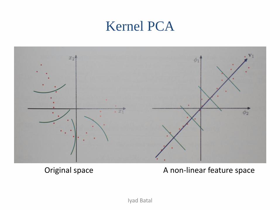
Kernel PCA

Original space A non-linear feature space

Iyad Batal

Isomap

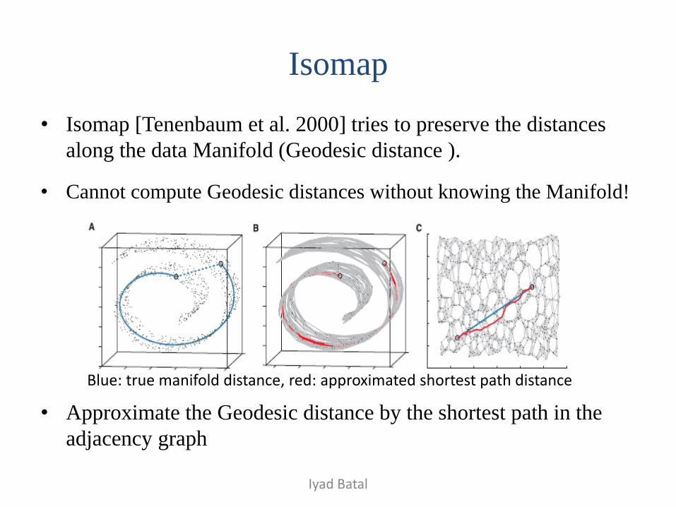
• Isomap [Tenenbaum et al. 2000] tries to preserve the distances

along the data Manifold (Geodesic distance ).

• Cannot compute Geodesic distances without knowing the Manifold!

• Approximate the Geodesic distance by the shortest path in the

adjacency graph

Blue: true manifold distance, red: approximated shortest path distance

Iyad Batal

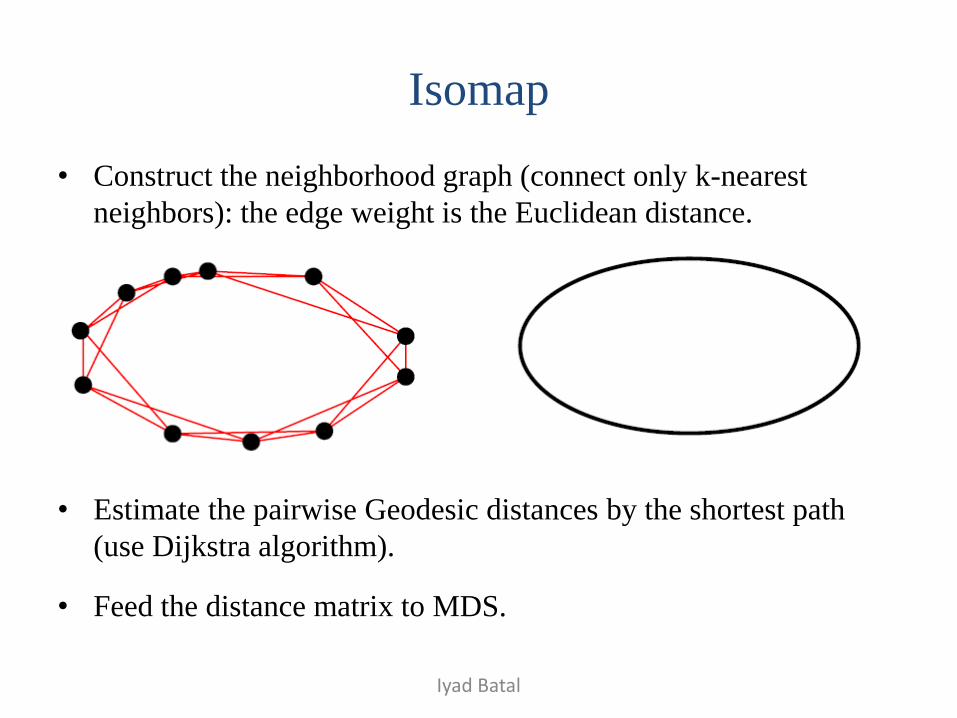
Isomap

• Construct the neighborhood graph (connect only k-nearest

neighbors): the edge weight is the Euclidean distance.

• Estimate the pairwise Geodesic distances by the shortest path

(use Dijkstra algorithm).

• Feed the distance matrix to MDS.

Iyad Batal

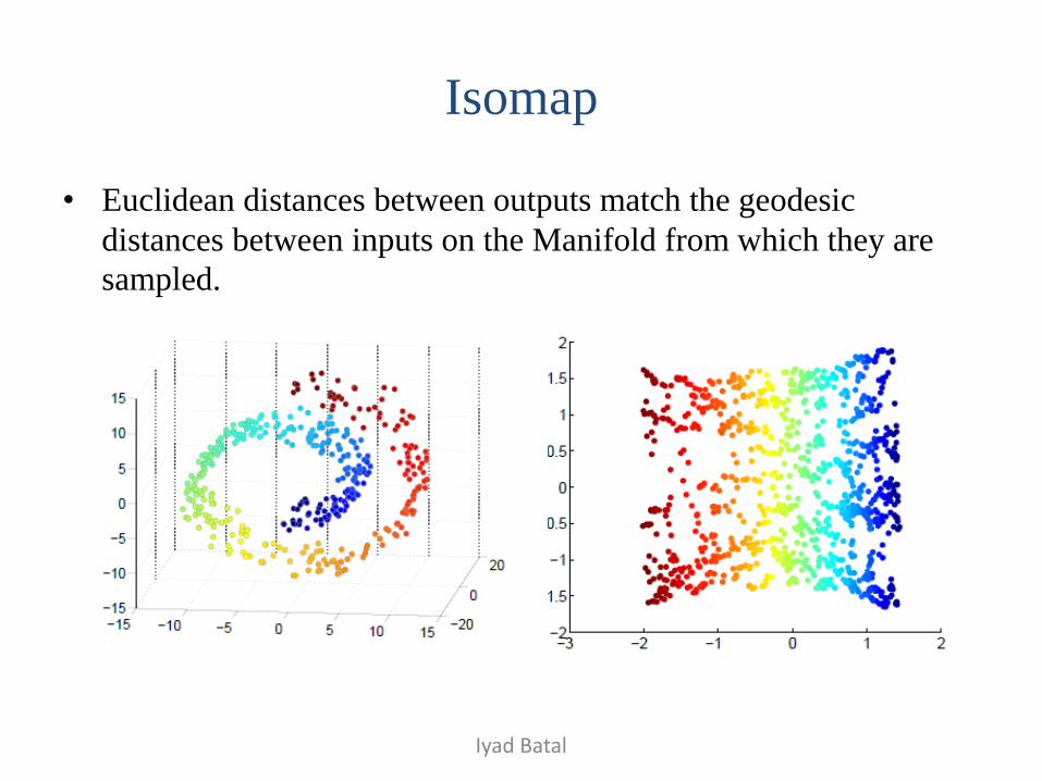
Isomap

• Euclidean distances between outputs match the geodesic

distances between inputs on the Manifold from which they are

sampled.

Iyad Batal

Related Feature Extraction Techniques

Linear projections:

• Probabilistic PCA [Tipping and Bishop 1999]

• Independent Component Analysis (ICA) [Comon , 1994]

• Random Projections

Nonlinear projection (manifold learning):

• Locally Linear Embedding (LLE) [Roweis and Saul, 2000]

• Laplacian Eigenmaps [Belkin and Niyogi, 2003]

• Hessian Eigenmaps [Donoho and Grimes, 2003]

• Maximum Variance Unfolding [Weinberger and Saul, 2005]

Iyad Batal