Principles and Applications of Molecular Dynamics Simulations with NAMD

NCSAsupercomputer

Computational Microscope

JC Gumbart Assistant Professor of Physics Georgia Institute of Technology gumbart@physics.gatech.edu simbac.gatech.edu

Nov. 14, 2016

These workshops started as one person’s dreamJune 2003, Urbana

Klaus Schulten 1947-2016

March 2011, Atlanta

Nov. 2014, Atlanta"We really feel that you cannot teach just by lecturing; you have to teach through hands-on examples.”

This is workshop #45 I’ve taught at workshops 4, 5, 8,

9, 10, 12, 14, 15, 20, 21, 34, 35

SIMBAC(simulations of bacterial systems) Lab at Georgia Tech

Biophysics Research at Georgia Tech

VERY, VERY SMALL!!!!

How small are the things we simulate?

can not even be seen with visible light!

can be counted in atoms!

MD simulations as a computational microscope

the traditional light microscope can barely see bacteria

the computational microscope can “see” everything with infinite resolution

Scalable molecular dynamics with NAMD. J. C. Phillips, R. Braun, W. Wang, J. Gumbart et al. J. Comp. Chem., 26:1781-1802, 2005.

010101000011101111010101010101010011101111010101101010111101

“Everything that living things do can be reduced to wiggling and jiggling of atoms.”

Richard Feynman (1963)

50 years later…But we are far from done!

State of the art

individual protein (500 atoms, 1977)

HIV virus capsid (64 million atoms, 2013)

Zhao, Perilla, Yufenyuy, Meng, Chen, Ning, Ahn, Gronenborn, Schulten, Aiken, Zhang. Mature HIV-1 capsid structure by cryo-electron microscopy and all-atom molecular dynamics. Nature, 497:643-646, 2013.

photosynthetic chromatophore (100 million atoms, 2016)

McCammon, Gelin, Karplus. Dynamics of folded proteins. Nature, 267:585-590, 1977.

Sener, Strumpfer, Singharoy, Hunter, Schulten. Overall energy conversion efficiency of a photosynthetic vesicle. eLife, 5:e09541, 2016.

“It is nice to know that the computer understands the problem. But I would like to understand it, too.”

Eugene Wigner

Why do we use MD?

We don’t simulate just to watch! But also to measure, analyze, and understand

Why do we use MD?

• Generating a thermodynamic ensemble (sampling / statistics)

• Taking into account fluctuations/dynamics in interpretation of experimental observables

• Describing molecular processes + free energy

• Help with molecular modeling

The Molecular Dynamics Simulation Process

For textbooks see:

M.P. Allen and D.J. Tildesley. Computer Simulation of Liquids.Oxford University Press, New York, 1987.  D. Frenkel and B. Smit. Understanding Molecular Simulations. From Algorithms to Applications. Academic Press, San Diego, California, 1996. A. R. Leach. Molecular Modelling. Principles and Applications.Addison Wesley Longman, Essex, England, 1996. More at http://www.biomath.nyu.edu/index/course/99/textbooks.html

Potential Energy (hyper)SurfaceE

nerg

y U

(x)

Conformation (x)

What is Force?

€

F = −ddxU(x)

Energy function:

used to determine the force on each atom:

yields a set of 3N coupled 2nd-order differential equations that can be propagated forward (or backward) in time.

Initial coordinates obtained from crystal structure, velocities taken at random from Boltzmann distribution.

Classical Molecular Dynamics at 300 K

van der Waals interaction

!!

"

#

$$

%

&

''(

)**+

,−'

'(

)**+

,=

6

min,

12

min, 2)(ij

ij

ij

ijij r

RrR

rU ε

ij

ji

rqq

rU04

1)(πε

=

Classical Molecular Dynamics

Coulomb interaction

tryptophan

€

U(r) =14πε0

qiqj

ri j+ εi j

Rmin,i jri j

$

% & &

'

( ) )

12

− 2Rmin,i jri j

$

% & &

'

( ) )

6+

,

- -

.

/

0 0

€

F(r ) = −1

4πε0

qiqj

ri j2 −12

εi jri j

Rmin,i j

ri j

%

& ' '

(

) * *

12

−Rmin,i j

ri j

%

& ' '

(

) * *

6+

,

- -

.

/

0 0

%

&

' '

(

)

* * ˆ r i j

Classical Molecular Dynamicstryptophan

Classical Molecular Dynamicstryptophan

Classical Molecular Dynamics

Bond definitions, atom types, atom names, parameters, ….

tryptophan

What is a Force Field?

To describe the time evolution of bond lengths, bond angles and torsions, also the non-bonding van der Waals and elecrostatic interactions between atoms, one uses a force field. The force field is a collection of equations and associated constants designed to reproduce molecular geometry and selected properties of tested structures.

In molecular dynamics a molecule is described as a series of charged points (atoms) linked by springs (bonds).

tryptophan

• Simple, fixed algebraic form for every type of interaction.

• Variable parameters depend on types of atoms involved.

heuristic

from physicsParameters: “force fields” like Amber, Charmm (note version number!)

Potential Energy Function of Biopolymers

We currently use CHARMM36

Bonds: Every pair of covalently bonded atoms is listed.

Angles: Two bonds that share a common atom form an angle. Every such set of three atoms in the molecule is listed.

Dihedrals: Two angles that share a common bond form a dihedral. Every such set of four atoms in the molecule is listed.

Impropers: Any planar group of four atoms forms an improper. Specific sets of four atoms in the molecule are listed.

Potential Energy Function of Biopolymers

Interactions between bonded atoms

))cos(1( δφφ −+= nKVdihedral

€

Vbond = Kb b − bo( )2€

Vangle = Kθ θ −θo( )2

Bond Energy versus Bond length

Po

ten

tial En

erg

y,

kca

l/m

ol

0

100

200

300

400

Bond length, Å

0.5 1 1.5 2 2.5

Single BondDouble BondTriple Bond

Chemical type Kbond bo

C-C 100 kcal/mole/Å 2 1.5 Å

C=C 200 kcal/mole/Å 2 1.3 Å

C=C 400 kcal/mole/Å 2 1.2 Å

Bond-angle (3-body) and improper (4-body about a center) terms have similar quadratic forms, but with softer spring constants. The force constants can be obtained from vibrational analysis of the molecule (experimentally or theoretically).

Bond potential

Vbond

=

Kb

(b� b0)2

Dihedral energy versus dihedral angle

Po

ten

tial En

erg

y,

kca

l/m

ol

0

5

10

15

20

Dihedral Angle, degrees

0 60 120 180 240 300 360

K=10, n=1K=5, n=2K=2.5, N=3

Dihedral potential

))cos(1( δφφ −+= nKVdihedral

dihedral-angle (4-body) terms come from symmetry in the electronic structure. Cross-term map (CMAP) terms in CHARMM force field are a refinement to this part of the potential

δ = 0 for all three

€

εi jRmin,i jri j

#

$ % %

&

' ( (

12

− 2Rmin,i jri j

#

$ % %

&

' ( (

6*

+

, ,

-

.

/ /

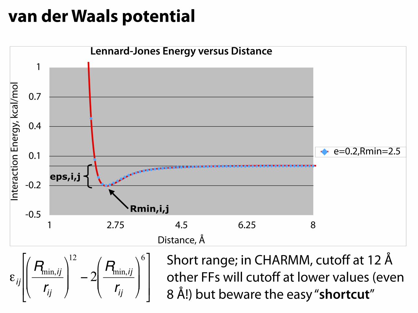
van der Waals potential

Short range; in CHARMM, cutoff at 12 Å other FFs will cutoff at lower values (even 8 Å!) but beware the easy “shortcut”

Lennard-Jones Energy versus Distance

Inte

ract

ion

Ener

gy, k

cal/m

ol

-0.5

-0.2

0.1

0.4

0.7

1

Distance, Å1 2.75 4.5 6.25 8

e=0.2,Rmin=2.5

Rmin,i,j

eps,i,j

-100.0000

-80.0000

-60.0000

-40.0000

-20.0000

0

20.0000

40.0000

60.0000

80.0000

100.0000

0 1.0000 2.0000 3.0000 4.0000 5.0000 6.0000 7.0000 8.0000

Electrostatic Energy versus DistanceIn

tera

ctio

n en

ergy

, kca

l/mol

Distance, Å

q1=1, q2=1 q1=-1, q2=1

From MacKerellNote that the effect is long range.

Coulomb potential

Equilibrium Properties of Proteins

Energies: kinetic and potential

Kinetic energy (quadratic)

Potential energy (not all quadratic)

?temperature dependence

Equilibrium Properties of Proteins

Energies: kinetic and potential

Kinetic energy (quadratic)

Potential energy (not all quadratic)

y/x ~ 1.7y/x ~ 0.6

y/x ~ 0.6

y/x ~ 2.9

http://www.ks.uiuc.edu/Research/vmd/plugins/fftk/

Force field toolkit (FFTK)

Mayne, Saam, Schulten, Tajkhorshid, and Gumbart. Rapid parameterization of small molecules using the force field toolkit. (2013) J. Comp. Chem. 34:2757-2770.

FFTK aids in the development of parameters in the MD potential function for novel molecules, ligands

Potential Energy (hyper)SurfaceEn

ergy

U(x

)

Conformation (x)

Classical Molecular Dynamics discretization in time for computing

Use positions and accelerations at time t and the positions from time t-δt to calculate new positions at time t+δt.

+

!“Verlet algorithm”

s

ms

μs

ns

ps

fs 100

106

109

1012

1015

103

Molecular dynamics timestep

bond stretching

steps

Hinge bending

Protein folding (typical)

Rotation of buried sidechains

Allosteric transitions

Protein folding (fastest)

Rotation of surface sidechains

The most serious bottleneck

SPEED LIMIT

δt = 1-2 fs*

*experimental 4-fs time steps with “hydrogen mass repartitioning” exists, but not in NAMD yet

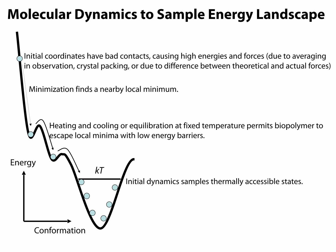
Molecular Dynamics to Sample Energy Landscape

Initial coordinates have bad contacts, causing high energies and forces (due to averaging in observation, crystal packing, or due to difference between theoretical and actual forces)

Minimization finds a nearby local minimum.

kTkT

kTkT

Initial dynamics samples thermally accessible states.

Energy

Conformation

Heating and cooling or equilibration at fixed temperature permits biopolymer to escape local minima with low energy barriers.

Longer dynamics access other intermediate states; one may apply external forces to access other available states in a more timely manner.

kT

kTkT

kTEnergy

Conformation

Molecular Dynamics to Sample Energy Landscape

2

)()0()(

i

iiA A

tAAtC =

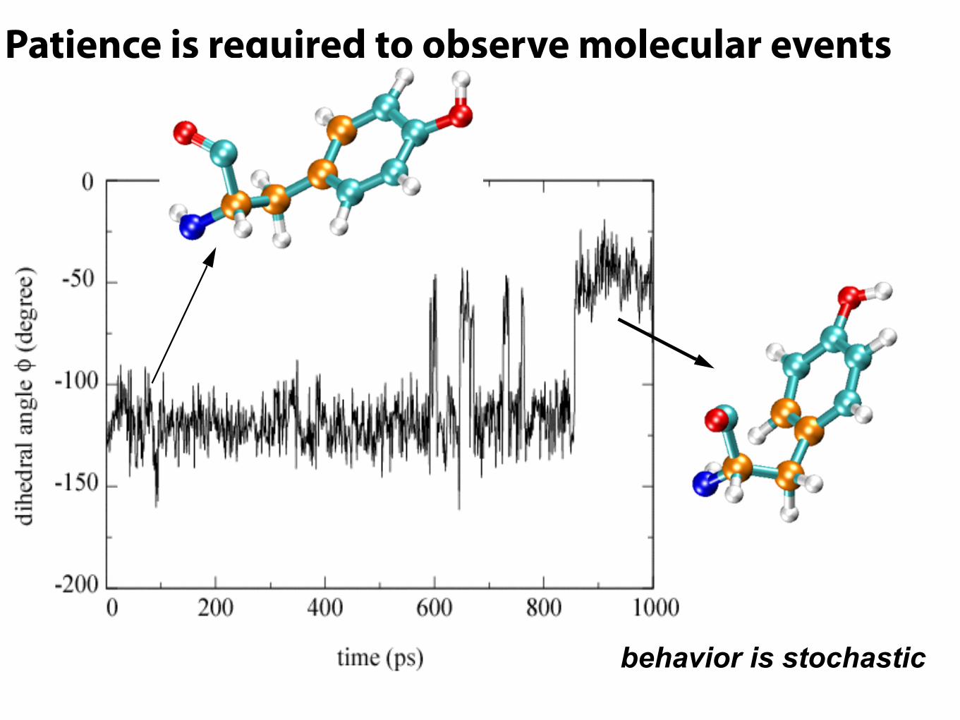
Patience is required to observe molecular events

Tyr35

behavior is stochastic

Patience is required to observe molecular events

DE Shaw et al. (2010) Science 330:341-346.

And there will always be a scale of dynamics you don’t observe!

Molecular Dynamics Ensembles thinking in terms of statistical mechanics

Constant energy, constant number of particles (NE; only if no periodic boundary conditions)

Constant energy, constant volume (NVE)

Constant temperature, constant volume (NVT)

Constant temperature, constant pressure (NPT)

Choose the ensemble that best fits your system and start the simulations - for most biomolecular systems, we choose NPT

-to simulate NVT (canonical) ensemble, need to duplicate the effect of a large thermal bath around the system

Temperature and Pressure control methods

-Damping (1/ps) should be enough to maintain temperature without significantly perturbing dynamics (5 is too much, 1 is probably okay)

Dynamics governed by the Langevin equation; gives the correct ensemble

random termdamping term

NPT (isobaric-isothermal) ensemble adds additional variables to control temperature, pressure which are ultimately integrated out to generate the correct distribution

In the simulation, pressure is calculated from the virial expansion

*For non-equilibrium simulations the Lowe-Andersen thermostat, which conserves momentum and does not suppress flows, may be preferred

Boundary Conditions?

What happens if you put water under vacuum!? Problems: Density, pressure, boundary effects, …

One solution: reflective boundaries, not quite good.

Spherical boundary conditions

Periodic Boundary Conditions

Maxwell Distribution of Atomic Velocities

Analysis of K, T (free dynamics)

The atomic velocities of a protein establish a thermometer.

Definition of temperature

NT32 2

2 =σ

ubiquitin in water bath

Root Mean Squared Deviation: measure for equilibration and protein flexibility

NMR structures aligned together to see flexibility

MD simulation The color represents mobility of the protein

through simulation (red = more flexible)

RMSD constant protein equilibrated*

Protein sequence exhibits characteristic permanent flexibility!

Equilibrium Properties of Proteins

Ubiquitin€

RMSD(t) =1N

Ri (t) −Ri (0)( )2i=1

N

∑*you never really know for sure

MD Results

RMS deviations for the KcsA protein and its selectivity filer indicate that the protein is stable during the simulation with the selectivity filter the most stable part of the system.

Temperature factors for individual residues in the four monomers of the KcsA channel protein indicate that the most flexible parts of the protein are the N and C terminal ends, residues 52-60 and residues 84-90. Residues 74-80 in the selectivity filter have low temperature factors and are very stable during the simulation.