PRINCIPLES AND PRACTICE OF COHERENT X-RAY · PDF file(MTF=modulation transfer function) Slide ... – Dedicated hard x-ray beam ... • The rays from the top and bottom of the object

ESRF Lecture Series on Coherent X-rays and their Applications, Lecture 7, Malcolm Howells

Henry Chapman, Anton Barty, Stefan Hau-Riege, Alex Noy

Lawrence Livermore National Laboratory

Malcolm Howells, Stefano Marchesini, JanosKirz, David Shapiro

Lawrence Berkeley National Laboratory

John Spence, Uwe Weierstall Arizona State University

Chris Jacobsen, Huijie Miao, Aaron Neiman, DavidSayre, Janos Kirz

Stony Brook University

PRINCIPLES AND PRACTICE OFCOHERENT X-RAY DIFFRACTION

IMAGING

Enju Lima, Lutz Wiegart, Malcolm Howells, AndersMadsen, Petra Pernot, Federico Zontone

European Synchrotron Radiation Facility


• Spatially andtemporallycoherent

• Monochromatic• 0.5-10 keV energy

undulator beamBiological or

materials sample

Diffraction pattern• To get a 2D image:- Record one diffraction pattern which gives Fourier amplitudes- Use a 2D phase retrieval algorithm to get their phases- Get an image by Fourier inversion

• To get a 3D image:- Record a tilt series of diffraction patterns- Insert the resulting Fourier amplitudes into a 3D Fourier space- Use a 3D phase retrieval algorithm to get their phases- Get an image by Fourier inversion (“true” 3D)

• True 3D is required when the collection angle includes a significantly curved portion of the Ewald sphere orwhen low-dose imaging is required

LENSLESS COHERENT X-RAY DIFFRACTIONIMAGING (CXDI)

CCD detector


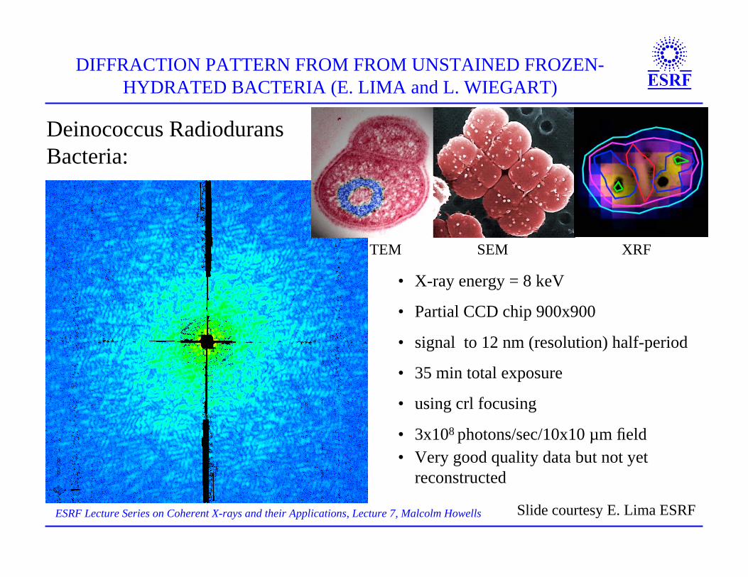
WHY IS “LENSLESS” ATTRACTIVE?• Zone-plate lenses waste x-rays which also hurts resolution when the imaging is damage limited• For example with 20 nm zone plates at the oxygen edge energy, we have 8x loss for diffraction

efficiency, 2x loss for window transmission, 5x loss for modulation transfer function (MTF) at 15nm feature size (graph below)

• Zone plates– are hard to make with good resolution– may have very short focal length (<1mm) which makes sample rotation hard– may have a depth of field less than the sample thickness → the image is not a projection

• Nevertheless zone-plate microscopes work and have many advantages and are viewed ascomplementary to diffractive imaging

(MTF=modulationtransfer function)

Slide: C. Jacobsen, Stony Brook


Thickness =100resolution elements

WHERE DOES CXDM FIT IN WITH OTHER 3DMICROSCOPES TODAY?


Sayre (1952) - Fundamentals of sampling the wave amplitude and wave intensity

Gerchberg and Saxton (1972) - First phase-retrieval algorithm successful on test data

Sayre (1980) - Idea to do "crystallography" with non-periodic objects (i. e. attempt phase retrieval) andexploit the cross-section advantage of soft x-rays

Sayre, Yun, Chapman, Miao, Kirz (1980’s and 1990’s) - development of the experimental technique

Fienup (1978-) - Development of practical phase-retrieval algorithms including use of the combinationof support constraint and oversampling of the amplitude pattern

Miao, Charalambous, Kirz and Sayre (1999) - first demonstration of 2-D CXDM using a Fienup-stylealgorithm at 0.73 keV x-ray energy, 75 nm resolution

Miao et al (2000) - imaging of a fixed biological sample in 2-D at 30 nm resolution

Miao et al (2001) - improved resolution in 2-D: 7 nmachievement of 3-D with moderate resolution: 55 nm

Robinson et al (2001-3) - Application to microcrystals and defects - 3D reconstruction - hardest x-rays

ALS group 2002-5 - reconstruction without use of other micoscopes - 3D reconstructions with many(up to 280) views and 10 nm resolution

COHERENT X-RAY DIFFRACTION IMAGING:HISTORY


ROOTS OF CXDI WERE IN THE US BUT IT IS NOWSPREADING MORE WIDELY

“Old” programs (>5years):• Brookhaven/Stony Brook

– Original concept and first experimental demonstration in 1999– Developed cryo CXDI for bio-samples– Now combined with the Berkeley/Livermore/Arizona-State effort at ALS

• UCLA/SSRL– User experiments at SPring8, 2D and 3D reconstructions– Resolution record 7 nm

• Advanced Photon Source– Dedicated hard x-ray beam line developed by University of Illinois– Microcrystal studies, 3D reconstructions

• Advanced Light Source: Arizona State, Lawrence Berkeley Lab, Lawrence Livermore Lab–3D with large numbers of views (up to 280) and 10 nm resolution

Newer programs:• SPring 8 – local program

• Swiss Light Source– New phasing methods

• BESSY– Holographic methods

• XFELs – DESY, LCLS– Damage-avoidance experiments

• ESRF– TROICA beam line - continuing development of cryo CXDI for bio-samples


3D IMAGE OF A MATERIALS-SCIENCE SAMPLE USINGCXDI (UCLA GROUP)

[Miao et al PRL 215503 (2006)]

• Surface rendering and through focus series of areconstructed 3D GaN "quantum dot" particle

• Resolution 17 nm

a) The front surface

b) The back surface

c) The side surface

d) The 3D internal structure showing regions oflow electron density (blue) corresponding to β -Ga2O3 and of high density corresponding to GaNcores


Robinson et al PRL, 87, 195505 (2001), Williams et al PRL, 90, 175501 (2003)

APPLICATION TO IMAGING NANOCRYSTALS

111 Bragg spot of 2 µm Aucrystal

Diffraction pattern around thespot (sampled at 30 planes)

Views of the reconstructedimage at nine depth values

SEM of nanocrystal


FIRST CDI RECONSTRUCTION USING ADEMONSTRATION OBJECT AT ESRF

• Image recorded in air at ID10C at 8 keV

• Negative pattern using 40 nm tungsten foil

• Diffraction pattern extended to 22 nm resolution

• Left: reconstructed CDI image

• Right: SEM imageSlide courtesy of E. Lima


MOVIE SHOWING PROGRESSIVE CONVERGENCE OFTHE ALGORITHM

Slide courtesy of E. Lima


FIRST CXDI IMAGE OF A BIOLOGICAL SAMPLE

• Imaging whole manganese-stained escherichia colibacteria at λ = 2Å, resolution 30 nm

• Beginning of a pathway toward imaging low-contrast biological objects

[Miao et al 2003]


LEFT: Reconstruction of freeze dried dwarf yeast at a single tilt orientation. A:

nucleus B: vacuole C: cell wall.

CENTER: STXM image of the same cell

RIGHT: movie of the nine reconstructions made

LOWER LEFT: Yeast cell diffraction pattern – 45 second total exposure –

speckles are visble out to the corners which correspond to 13.4 nm spatial period

(David Shapiro thesis project, work of SUNY/BNL and Cornell groups (PI’s Kirz,

Jacobsen, Cao, Elser))

FREEZE-DRIED-YEAST-CELL RECONSTRUCTIONS1 µm


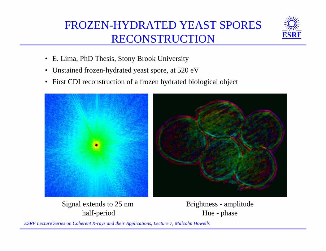
FROZEN-HYDRATED YEAST SPORESRECONSTRUCTION

Brightness - amplitudeHue - phase

• E. Lima, PhD Thesis, Stony Brook University• Unstained frozen-hydrated yeast spore, at 520 eV• First CDI reconstruction of a frozen hydrated biological object

Signal extends to 25 nm half-period


FAR-FIELD DIFFRACTION

• In the far-field the x axis is a mapping of spatial frequency according to

• The rays from the top and bottom of the object interfering at P produce Young’s intensityfringes with a frequency W /(λz) - This is the highest frequency that can be present in thediffraction pattern

• According to the Shannon Sampling theorem the pattern (i. e. |F(k)|2) must be sampled attwice that frequency in order to allow exact recovery of the pattern from the samples

• In other words a sampling interval of is needed to avoid loss of information

kP = sin! " # xP "z( )

12

!zW

Object f(x)which is non-zero onlybetween thebounds ofspacing W(known as the“support”)

Diffractionpatternproportional to|F(k)|2 whereF(k) is thetransform of f


MORE ABOUT SAMPLING• In general the Shannon sampling theorem (aka the Kotelnikov theorem) states that,

if a function f(x) with transform F(k) is bounded on one side with width W, then thefunction on the other side can be fully recovered from samples spaced at 1/W

• Thus if f is bounded by W then the sampling interval for F(k) should be

• This is to be compared with the result from the last slide

• Thus the Shannon sampling interval for the wave amplitude is twice that for thewave intensity

!k "!x#z

=1W

or !x[ ]F =#zW

!x[ ] F 2 =12"zW

Therefore if the intensity pattern (|F|2) is correctly (Shannon) sampled(i. e. not oversampled), and those data are used to get |F|, then |F| willautomatically be oversampled by a factor two in each dimension

ESRF Lecture Series on Coherent X-rays and their Applications, Lecture 7, Malcolm HowellsESRF Lecture Series on Coherent X-rays and their Applications, Lecture 7, Malcolm Howells

IN CRYSTALLOGRAPHY IT WOULD BE USEFUL TO KNOW |F|2 AT HALF-INTEGRALMILLER INDICES (TWICE-BRAGG SAMPLING) AND IN OPTICS YOU CAN!


Object f x( ) ! F k( ) "SHANNONF

=#zW

$%&

'()

(width W )

Autocorrelation f x( )* f x( ) ! F k( )2 "SHANNON

F 2

=#z2W

(width 2W )

CONSEQUENCES OF SHANNON SAMPLING THE INTENSITY

• Therefore |F| derived from intensity data is twofold oversampled compared to itsShannon frequency (in each dimension)

• This means that f derived by transforming F will be zero padded to a width 2W

• The zero-padded region allows "the support constraint" to be used

• This means that the algorithm is told that the electron density of the sample outsidesome given boundary is zero

• It seeks a solution for the phases of F in which (a) the support constraint is true inobject space and (b) the measured values of |F| are true in diffraction space

Shannon samples

2× oversampled

Experiment

Algorithm


OBJECT SPACEf(x)

FOURIER SPACEF(k)

Measured data

Add randomphases

First estimate of f(x)designated by g1(x)

gi(x) Gi(k)

gi+1(x)

FFT

1

4

2

FFT-1

3G′i(k)g′i(x)

Fourier domain constraints

Object domain constraints

Starting pointFFT-1

PHASE-RETRIEVAL ALGORITHMS: GENERAL SCHEME

IN

OUT

ith iteration


FIENUP HYBRID-INPUT-OUTPUT ALGORITHM STEPS

• S is the set of object domain points at which the object domain constraints are violatedand β is a number normally between 0.5 and 1.0

• In the reconstructions from ALS and ESRF shown here, only this algorithm has been used

• The constraints we have used in the work reported here1. Object domain: support constraint (object must be zero outside an adaptive boundary)2. Fourier domain: Fourier amplitude equals the square root of the measured intensity

• We used no other constraints or prior knowledge - only the measured diffraction pattern

Step 1 : Gi k( ) = Gi k( ) exp i!i k( )"# $% = FFT gi x( )"# $%

Step 2 : &Gi k( ) = F k( ) exp i!i k( )"# $%

Step 3 : &gi x( ) = FFT'1 &Gi k( )"# $%

Step 4 : gi+1 x( ) =&gi x( ) x ( S

gi x( ) ' ) &gi x( ) x * S+,-

INPUT

OUTPUT

Dainty and Fienup 1985, S. Marchesini, A unified evaluation of iterative projectionalgorithms for phase retrieval Rev. Sci. Instrum. 78, 011301 (2007)

ESRF Lecture Series on Coherent X-rays and their Applications, Lecture 7, Malcolm HowellsESRF Lecture Series on Coherent X-rays and their Applications, Lecture 4, Malcolm Howells

• One can show that the speckles will not be significantly blurred if the full-anglespread of the illuminating beam Δϑ satisfies Δϑ.2W = λ/2 [Spence et al 2004] - Wand λ are known

• This is a spatial coherence condition that says roughly that the sample plus the zero-padded area has to be coherently illuminated

• Choose a pinhole (or equivalent set of slits) of width about 2W

• Choose a distance downstream of the pinhole at which the beam has widened(diffracted by Δϑ) to about three or four pinholes diameters and place the sample(place guard slits in between the pinhole and sample)

• The idea is that the beam will be wide enough that the sample will stay in the beameven when displaced by the run-out of the rotation stage but not so wide that a lot offlux is lost

• Note that it is not necessary that the beam is a single mode - only that whatever partis used to illuminate the sample plus zero-padded area should be single mode

DESIGNING THE EXPERIMENT I: ARRANGING FOR SPATIALLYCOHERENT ILLUMINATION OF THE SAMPLE


Monochromaticity:1. Assume that the detector has NxN pixels each of width equal to the Shannon interval Δs = λz/(2W)2. Also from the diagram θ = NΔs/(2z)3. The greatest (worst case) path difference between two interfering signals at the detector edge is Wθ4. To ensure at least 50% overlap of the interfering wave trains we must require the coherence length

λ2/(Δλ) ≥ 2Wθ so substituting we get

W!

N!s 2

DESIGNING THE EXPERIMENT II: TEMPORALCOHERENCE (MONOCHROMATICITY) REQUIREMENTS

!

"!#

2W$

!=

2W!

N"s

2z=

2W!

N2z

!z2W

=N2

or !

"!#

N2

X-RAYS

Detector edge


3 keV is sufficient for 10-20 µm objects of biological density but there is asize/density region that needs a higher energy

1-µm objects

DESIGNING THE EXPERIMENT III: CHOICE OFWAVELENGTH

..


FLUX CONSIDERATIONS:

• The exposure time on a given source increases like E4 - conclusion: use lowest possible energy

DOSE CONSIDERATIONS:

• The dose for light elements (biology say) is roughly flat with wavelength

DIFFRACTION CONSIDERATIONS:

• For a maximum diffraction angle of 15° (Bragg angle of 7.5°) - 2.5 keV (0.5 nm wavelength) is enoughto get to 1 nm resolution

RECONSTRUCTION CONSIDERATIONS

• Harder x-rays will make the scattering factors essentially real which favors higher-energy x-rays

COMPUTER POWER

• 3D reconstruction is also limited by computer power - currently 10 hours for (1k)3 - this should reducethe demand to measure big objects

DESIGNING THE EXPERIMENT III: CHOICE OF WAVELENGTH(continued)


ALS BEAM LINE 9.0.1: COHERENT OPTICS

RATIONALE:• Experiments have been done at 520, 750 and 1500 eV in undulator 3rd harmonic• Be window is 0.8 mm diameter which defines the beam size• XPCS users originally required pink beam so zone plate mono is retractable• Resolving power of 500-1000 is required (compared to ≈100 for the pink beam)

multilayer/specular

mirror (3°)


THE STONY BROOK DIFFRACTION CHAMBER ALLOWSACCURATE SAMPLE ROTATION AND DATA ACQUISITION

Stony Brook diffraction chamber(Chris Jacobsen and Janos Kirz)

Installed at ALS BL9.0.1


Drive 1Drive 3

Drive 2

Drive 4

Drive 5

DIFFRACTION CHAMBER OPTICAL ELEMENTS

150 mm

25 mm

Slide courtesy D. Shapiro


NATURAL COCCOLITH SAMPLE - HOW DO WE KNOWWE ARE REALLY ILLUMINATING THE SAMPLE

• Coccolith, calcite shields producedby unicellular marine algae(haptophytes) (SEM picture)

• The sample was placed on a Si3N4membrane with focused ion beam(FIB).

• The dot on the up right corner is adeposited platinum tower about 100nm diameter and 400 nm high

• The dot can be as a reference forFourier transform holography

A diffraction pattern (Fouriertransform hologram in this case)taken with an exposure time of 20seconds

Autocorrelation function of theleft pattern


GATAN 630 CRYO HOLDER

High-tilt cryo holder for JEOL TEM which allows use of special slotted samplegrid that allows tilts to ±80° without obstructing the beam or spilling the LN2

Slide: courtesy T. Beetz, Xradia


JEOL TEM GONIOMETER: SCHEMATIC

Slide: courtesy T. Beetz, Xradia


Grids with live cells are• Taken from culture medium and blotted• Plunged into liquid ethane (cooled by liquid nitrogen) to freeze the water in the

sample to vitreous ice (at ESRF a home made plunger (Lima/Wiegart) is used)• Loaded into cryo holder• Concerns exist about how large a sample can be vitrified in this way• People move from electron techniques to x-ray to look at bigger samples - but

how big can they be and still plunge freeze successfully?• It may be necessary to turn to pressure freezing which can work slowly and can

still freeze big objects (>0.1 mm)

ELECTRON SAMPLE PREPARATION METHODS FORBIOLOGICAL SAMPLES AS USED AT ALS

Slide: A. Stewart (Stony Brook)


FROZEN HYDRATED: STABLE SPECIMENS!

Frozen hydrated specimensdon’t shrink in the beam (freeze-dried specimens do)‏

(David Shapiro, PhD dissertation, Stony Brook, 2004)

Reconstructed freezedried yeast cell

Slide: courtesy A. Stewart (Stony Brook)


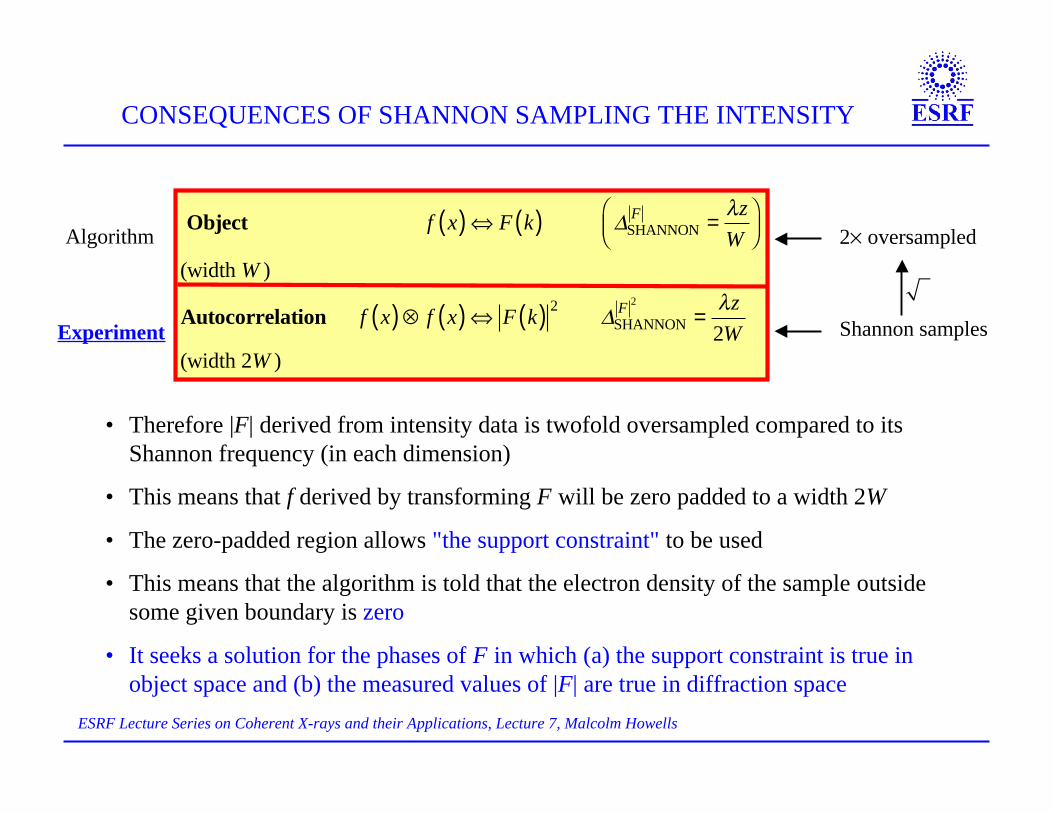
DIFFRACTION PATTERN FROM FROM UNSTAINED FROZEN-HYDRATED BACTERIA (E. LIMA and L. WIEGART)

• X-ray energy = 8 keV

• Partial CCD chip 900x900

• signal to 12 nm (resolution) half-period

• 35 min total exposure

• using crl focusing

• 3x108 photons/sec/10x10 µm field• Very good quality data but not yet

reconstructed

Deinococcus Radiodurans Bacteria:

TEM SEM XRF

Slide courtesy E. Lima ESRF


DATA ACQUISITION IN AIR USING 8KEVX-RAYS (E. LIMA and L. WIEGART

• Data taken at ID10C mostly at8 keV

• Frozen samples are protectedfrom ice contamination withincryostream

• Samples are monitored betweendata-taking runs by on-axislight microscope

Vacuum



Nylon sample loopRed square=ID14 beam size

(100x100 µm2)

Powder diffraction at 13 keVID14, ESRF

Powder diffraction data demonstrates vitreous ice after plunge-freezing

SAMPLE PREPARATION AND MOUNTING (E. LIMA and P. PERNOT)



DEMONSTRATION OF HIGH-RESOLUTION CXDI ON AGOLD-BALL SAMPLE

• Sample: 50 nm gold spheres• Diffraction recorded with undulator radiation, λ = 1.6 nm• Rayleigh resolution of reconstructed image: 10 nm• Reconstruction performed with Shrinkwrap: a variation of Fienup-hybrid-input-

output algorithm, with dynamic support constraint [S. Marchesini et al PRB 2003]

X-ray image(reconstruction)

SEM image

300 nm

X-ray diffraction pattern


LENSLESS IMAGING WITH THE“SHRINKWRAP” ALGORITHM

Scanning electronmicroscope image

First estimate of the object:thresholded autocorrelation function

(transform of the measured data)

First estimate of thesupport function

Stopping criterion

0 500 1000 1500 2000Iteration

0.0

0.2

0.4

0.6

Supportconstrainterror

Marchesini et al., Phys. Rev. B 68 140101, (2003)


WE MANUFACTURED A COMPACT 3D TESTOBJECT

1 µm

Silicon nitride pyramiddecorated with Auspheres

X-ray diffraction pattern

Silicon nitridemembrane

Silicon

SEM image

50 nm goldballs

Lawrence Livermore Lab group:


FULL 3D X-RAY RECONSTRUCTION OF NON-CRYSTALLINEMATERIAL AT HIGH RESOLUTION - ANTON BARTY, LLNL

Complete image reconstruction achieved,without any prior knowledge, usingShrinkwrap, parallelized for 3D on 16-nodecluster.

Coherent X-ray diffraction data, rotatingthe sample -57 to +65 degrees (5×108

data points)

Slide courtesy A. Barty LLNL


WITH A FULL 3D RECONSTRUCTION IN HAND WE CAN GETREAL-SPACE PROJECTIONS USING A SLICE THROUGH k-SPACE

SEM image of 3D pyramid testobject

Projected views from the 3D reconstruction

Anton Barty, LLNL



-1000 -900 -800 -700y (nm)

-5

0

5

10

15

20

MEASURES OF RESOLUTION: REAL SPACE

0 100 200x (nm)

-5

0

5

10

15

20

-200 -100 0 100y (nm)

-5

0

5

10

15

20

800 900 1000z (nm)

-5

0

5

10

15

20

One50 nmball

x y z

41 nm

50 nm

75 nmIm

age

ampl

itude

3 orthogonalline-outs of asingle 50 nmball

Three50nm balls

Line-outs ofthree ballsin a row

45 nm

H. Chapman et al, J.Opt. Soc. Am. A 23,1179-1200 (2006)

Imag

e am

plitu

deSlide courtesy H. Chapman LLNL


THE CONSISTENCY OF THE RECONSTRUCTEDPHASES CAN BE QUANTIFIED

Is the solution unique? Can we determine a confidence of the reconstructed phases?

According to Veit Elser (Cornell) the answer is average the complex amplitudes of manyreconstructions with different random starts, then compare |<F>|2 to measured intensity. Ifphase recovery of particular pixels is unsuccessful they will return random results and willaverage to near zero. If recovery of is good they will return consistent results similar to |<F>|2

�

F(q)2

I(q)= cos! 2

0.00 0.01 0.02 0.03 0.04 0.05 0.06q (1/nm)

0.0

0.2

0.4

0.6

0.8

1.0We define an "algorithmtransfer function" for 2Dprojection by averagingrandom starts

14 nm period - 7 nm half-period

CENTER EDGE CORNER

10 nm half-period

Slide: courtesy S. Marchesini, LBNL


3D IMAGE RECONSTRUCTIONS FROM EXPERIMENTAL X-RAYDATA (by Anton Barty of LLNL)

304 GB176 GB20483

38 GB4.7 Gb

592 MB

DoublePrecision

22 GB2.6 GB336 MB

SinglePrecision

Memory needed

2563

10243

5123

Size

????20483

14 hrs1.5 hrs10 mins

Processingtime*

8 sec850 msec73 msec

3D FFT timing

32-CPU G5 cluster speed

2563

10243

5123

Size

ReconstructionVoxel Data cube 10243 elements

Iterative reconstruction algorithm a few 1000s of 3D FFTs required

*2000 iterations, 2FFTs per iteration plus other floating point operations code: C with mvapich, dist_fft (Altivec-optimized MPI FFT) see http://images.apple.com/acg/pdf/20040827_GigaFFT.pdf



• [Barty et al PRL 2008 (inpress), preprint - http://arxiv.org/abs/0708.4035v1]

• Ta2O5 aerogel (0.1 gm/cm3),(bulk density = 8.5 gm/cm3)

• Reconstructed images alongorthogonal views

• Reconstruction details: 3D HIOwith β = 0.9 for 300 iterationswith support refinementfollowed by RAAR (relaxedaveraged alternatingreflections) algorithm [D. R.Luke 2005] (also with β = 0.9)through to iteration 2000

SEM image

yx

yz

zx

membrane

membrane

Slide: A. Barty, LBNL

INVESTIGATION OF A 2µm AEROGELSTRUCTURE


3D AEROGEL RECONSTRUCTION(by A. Barty LLNL)

1 micron


500 nm

Mechanical analysis: J.Kinney (LLNL)

THE 3D AEROGEL IMAGES REVEAL ITSSKELETON STRUCTURE

Electron microscopeexamination of a thinportion near a sampleedge - only a few thesecan be found thin enough


Small angle x-ray scattering data calculated from the 3D volumereconstruction (XDI) compared to ultra small angle x-ray scattering(USAXS) measurements [Ilavski et al 2002, 2004 (SRI)] on a similarbatch of 100 mg/cc Ta2O5 aerogel

[Barty et al PRL 2008 (in press)]

COMPARISON OF AEROGEL RESULTS WITH USAXS-MEASUREDDATA


Present beam line

• 280 views ±70° at 0.5° intervals - resolution 10 nm - sample density = 0.1 gm/cc

• Total time taken - 24 hours of which 8 hours is set-up, 8 hours exposing, 8 hrs overhead tasks

COSMIC beam line: superior flux on sample to present one by:

• Factor 15 due to ALS upgrade and optimised undulator brightness

• Factor 5 due to getting stigmatic BL optics (this has recently been done)

• Factor 6 due to improved component efficiencies - pinhole especially

• Overall factor 450

• Assume we are no longer limited by detector readout

• We project nm resolution in 8 hours or 10 nm in a 1 minute exposure

• This improvement of resolution means 450 time more dose!!!

10 4504 = 2.1

Aerogel sample: Estimateof resolution by thealgorithm transferfunction is 10 nm

PROJECTED RESOLUTION AND EXPOSURE TIMEFOR A NEW BEAM LINE (ALS "COSMIC" PROJECT)


R. Hegerl and W. Hoppe, Zeitschrift Naturforsch 3a, 1717-1721 (1976), Abstract:

• “A three-dimensional reconstruction requires the same integral dose as a conventional two-dimensional micrograph provided that the level of (statistical) significance and theresolution are identical. The necessary dose D for one of the K projections in areconstruction series is, therefore, the integral dose divided by K”

• The discussion provided by the originators of the theorem was largely in terms of a singlevoxel but, as pointed out by McEwan et al 1995, the conclusion can be immediatelygeneralized to a full 3D object by recognizing that conventional tomographic projectionsare linear superpositions of the contributions of the individual voxels. A similar argumentin frequency space shows that the theorem also applies to CXDI.

• Study by B. McEwan, K. Downing, R. Glaeser Ultramicroscopy 60, 357-373 (1995)extended the validity to cases with:– high absorption– signal-dependent noise– varying sample contrast– missing angular range– a need to align the recorded patterns by cross-correlation methods

THE DOSE FRACTIONATION THEOREM OF STANDARDTOMOGRAPHY


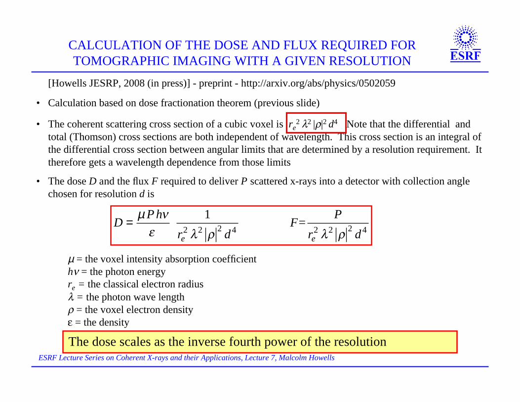
• Calculation based on dose fractionation theorem (previous slide)

• The coherent scattering cross section of a cubic voxel is re2

λ2 |ρ|2 d4 Note that the differential andtotal (Thomson) cross sections are both independent of wavelength. This cross section is an integral ofthe differential cross section between angular limits that are determined by a resolution requirement. Ittherefore gets a wavelength dependence from those limits

• The dose D and the flux F required to deliver P scattered x-rays into a detector with collection anglechosen for resolution d is

D =µ P h!"

1re

2 #2 $2 d4

F= Pre

2 #2 $2 d4

µ = the voxel intensity absorption coefficienthν = the photon energyre = the classical electron radiusλ = the photon wave lengthρ = the voxel electron densityε = the density

The dose scales as the inverse fourth power of the resolution

CALCULATION OF THE DOSE AND FLUX REQUIRED FORTOMOGRAPHIC IMAGING WITH A GIVEN RESOLUTION

[Howells JESRP, 2008 (in press)] - preprint - http://arxiv.org/abs/physics/0502059


MEASUREMENT OF THE POWER LAW

Exposure time scales as the fourth power of the spatial frequency

• Record diffractionpatterns with a widerange of exposure times1-512s

0

0.5

1

1.5

2

2.5

0 0.1 0.2 0.3 0.4 0.5 0.6Log(F/F0)

log(

T/T0

)

slope=3.94+/-0.12intercept=-0.05+/-0.04

Freeze dried yeast at Beamline 9.0.1

• Fit polynomial to powerspectrum

• Determine limiting spatialfrequency where scatteredpower drops to noise

• Plot limiting spatialfrequency versus singleshot exposure time

Slide courtesy D. Shapiro

Slope=4


FLUX REQUIREMENTS

Flux to get 25 scattered x-rays per voxel, voxel size (Å) = 100

1.0E+07

1.0E+08

1.0E+09

1.0E+10

1.0E+11

1.0E+12

1.0E+13

100 1000 10000

Energy (eV)

Flux

(ph/

µm

^2)

Protein against abackground of water

Protein alone

Flux to detect a 10 nm voxel made of protein according to the Rose criterion.A detector collecting an angle chosen for 10 nm resolution is assumed

Note the square-law increase of requiredflux with x-ray energy - this combinedwith the square law decrease ofavailable coherent flux with energy for asource of a given brightness leads tofourth-power loss of flux whenunnecessarily high x-ray energy is used


Below is the dose to detect a 10 nm voxel made of protein according to theRose criterion. A detector collecting an angle chosen for 10 nm resolution isassumed

DOSE REQUIREMENTS

Dose to get 25 scattered x-rays per voxel, voxel size (Å) = 100

1.0E+06

1.0E+07

1.0E+08

1.0E+09

1.0E+10

1.0E+11

100 1000 10000

Energy (eV)

Dose

(G

y)

Protein against abackground of water

Protein alone


DIFFRACTION SPOT-FADING EXPERIMENT ONALS BEAM LINE 8.3.1 (J. HOLTON)

• Ribosome crystals (J. Cate)

• About 24 hour exposure at 10 keV

• Long "dosing" exposures with slits wide were alternated with shorter"measurement" exposures with slits narrow

[Howells et al JESRP 2008 in press]


DOSE-RESOLUTION RELATIONSHIP FOR 3D IMAGING OFFROZEN-HYDRATED SAMPLES

Every bond brokenabove here

X-rays:Glaeser et al 2000Gonzales et al 1992Sliz et al 2003Burmeister 2000Schneider 1998Henderson 1990Maser et al 2000

Electrons:Glaeser and Taylor 1978Plitzko et al 2002Hayward and Glaeser 1979

Mostly crystallography

X-ray microscopy

ALS BL 7.3.3, Glaeser ALS BL 8.3.1, Holton

1011


Summary of conclusions from the graph on the last slide• This calculation applies to diffraction by natural (unlabelled) protein against a background of

water.

• Diffraction imaging experiments are only possible in the pink triangle to the right.

• According to the Rose criterion the dose-limited resolution by CXDI under the given conditionsis predicted to be 10 nm.

• The quoted electron and x-ray results for the maximum tolerable dose agree well as we believethey should.

• The fourth-power dependence of dose on resolution is obtained by both calculation andexperiment - straightness of the dose resolution plot for a particular sample offers a possible testfor the onset of damage.

• The dose is expected to have only a weak dependence on x-ray energy.

• The calculation predicts what is already generally believed - that at least 1011 copies of thesample are required to solve a structure crystallographically to atomic resolution.

• Possible strategies for overcoming the 10-nm limit include (i) the use of labelling to improve thecontrast and thus the resolution for a given tolerable dose and (ii) the use of samples with moreorder (prior knowledge) than a cell of completely unknown structure, for example fibers.

SUMMARY AND CONCLUSIONS ON DOSE ANDDAMAGE


CALCULATION OF EXPOSURE TIME FOR A 2D IMAGE WITH ROSE-CRITERION IMAGE QUALITY FOR COHERENT X-RAY DIFFRACTION

MICROSCOPY

Using coherent flux =B ! 2( )2

and fractional BW=1/(N /2), we get

T =2PA

re2!4 "eff

2d4KB

B is the brightness in usual units, K is thedetector resolution in reciprocal kilopixelseg a 4000 pixel detector has K=0.25 - Kdetermines the BW, A is the sample area

ASSUMPTIONS:• Lossless beam line• A coherent (single-mode) beam is exactly delivered to fill the sample area• Number of scattered x-rays per pixel P = 25 (Rose criterion)• Parameter values: A=10x10µm2, |ρeff|2 is for protein against a background of water, d=10 nm,

K=1 (1000x1000 detector) and B=1019 usual units• Note that for a given source brightness the exposure time increases roughly as (energy)4

Documents

PRINCIPLES AND PRACTICE OF COHERENT X-RAY · PDF file(MTF=modulation transfer function) Slide ... – Dedicated hard x-ray beam ... • The rays from the top and bottom of the object