Principles of Ground water flow - IITs and IISc elearning Courses

Module 2

The Science of Surface and Ground Water

Version 2 CE IIT, Kharagpur

Lesson 6

Principles of Ground Water Flow


Instructional Objectives On completion of the lesson, the student shall be learn

1. The description of steady state of ground water flow in the form of Laplace equation derived from continuity equation and Darcy’s law for ground water movement.

2. The quantitative description of unsteady state ground water flow. 3. The definition of the terms Specific Yield and Specific Storage and their

relationship with Storativity of a confined aquifer. 4. The expressions for ground water flow in unconfined and confined

aquifers, written in terms of Transmissivity. 5. Expression for two – dimensional flow in unconfined and confined

aquifers; Boussinesq equation. 6. Expression for two – dimensional seepage flow below dams. 7. Analytical solution of steady one dimensional flow in simple cases of

confined and unconfined aquifers.

2.6.0 Introduction In the earlier lesson, qualitative assessment of subsurface water whether in the unsaturated or in the saturated ground was made. Movement of water stored in the saturated soil or fractured bed rock, also called aquifer, was seen to depend upon the hydraulic gradient. Other relationships between the water storage and the portion of that which can be withdrawn from an aquifer were also discussed. In this lesson, we derive the mathematical description of saturated ground water flow and its exact and approximate relations to the hydraulic gradient. 2.6.1 Continuity equation and Darcy’s law under steady state conditions Consider the flow of ground water taking place within a small cube (of lengths ∆x, ∆y and ∆z respectively the direction of the three areas which may also be called the elementary control volume) of a saturated aquifer as shown in Figure 1.


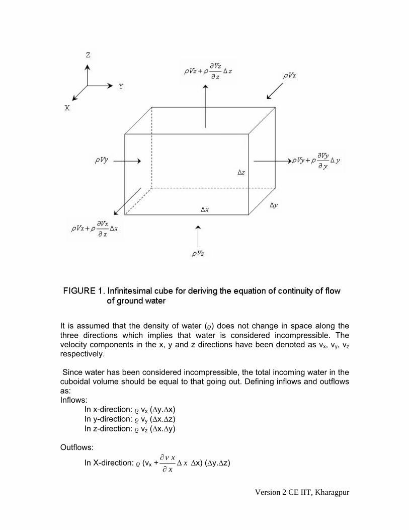
It is assumed that the density of water (ρ) does not change in space along the three directions which implies that water is considered incompressible. The velocity components in the x, y and z directions have been denoted as νx, νy, νz respectively. Since water has been considered incompressible, the total incoming water in the cuboidal volume should be equal to that going out. Defining inflows and outflows as: Inflows:

In x-direction: ρ νx (∆y.∆x) In y-direction: ρ νy (∆x.∆z) In z-direction: ρ νz (∆x.∆y)

Outflows:

In X-direction: ρ (νx + xxx

Δ∂

∂ν ∆x) (∆y.∆z)


In Y-direction: ρ (νy+ yyy

Δ∂

∂ν) (∆x.∆z)

In Z-direction: ρ (νz+ zz

∂∂ν

.∆z) (∆y.∆x)

The net mass flow per unit time through the cube works out to:

⎥⎦

⎤⎢⎣

⎡∂

∂+

∂∂

+∂

∂zyx

zyx ννν (∆x.∆y.∆z)

Or

zyxzyx

∂∂

+∂

∂+

∂∂ ννν

= 0 (2)

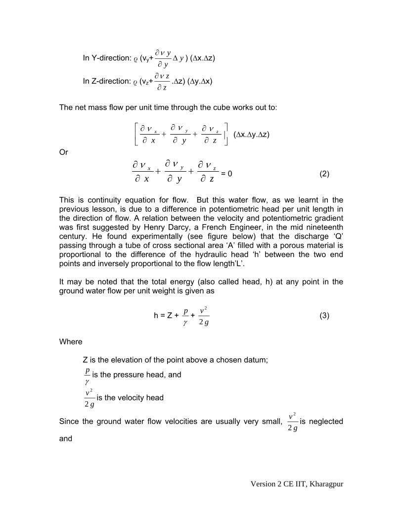
This is continuity equation for flow. But this water flow, as we learnt in the previous lesson, is due to a difference in potentiometric head per unit length in the direction of flow. A relation between the velocity and potentiometric gradient was first suggested by Henry Darcy, a French Engineer, in the mid nineteenth century. He found experimentally (see figure below) that the discharge ‘Q’ passing through a tube of cross sectional area ‘A’ filled with a porous material is proportional to the difference of the hydraulic head ‘h’ between the two end points and inversely proportional to the flow length’L’. It may be noted that the total energy (also called head, h) at any point in the ground water flow per unit weight is given as

h = Z + γp +

gv2

2

(3)

Where

Z is the elevation of the point above a chosen datum;

γp is the pressure head, and

gv2

2

is the velocity head

Since the ground water flow velocities are usually very small, g

v2

2

is neglected

and


h = Z+γp is termed as the potentiometric head (or piezometric head in some

texts)

Thus

Q α A • ⎟⎟⎠

⎞⎜⎜⎝

⎛ −

Lhh QP (4)

Introducing proportionality constant K, the expression becomes

Q = K.A. ⎟⎟⎠

⎞⎜⎜⎝

⎛ −

Lhh QP (5)

Since the hydraulic head decreases in the direction of flow, a corresponding differential equation would be written as

Q = -K.A. ⎟⎠⎞

⎜⎝⎛

dldh (6)

Where (dh/dl) is known as hydraulic gradient. The coefficient ‘K’ has dimensions of L/T, or velocity, and as seen in the last lesson this is termed as the hydraulic conductivity.


Thus the velocity of fluid flow would be:

ν = AQ = -K (

dldh ) (7)

It may be noted that this velocity is not quite the same as the velocity of water flowing through an open pipe. In an open pipe, the entire cross section of the pipe conveys water. On the other hand, if the pipe is filed with a porous material, say sand, then the water can only flow through the pores of the sand particles. Hence, the velocity obtained by the above expression is only an apparent velocity, with the actual velocity of the fluid particles through the voids of the porous material is many time more. But for our analysis of substituting the expression for velocity in the three directions x, y and z in the continuity relation, equation (2) and considering each velocity term to be proportional to the hydraulic gradient in the corresponding direction, one obtains the following relation

0=⎟⎠⎞

⎜⎝⎛

∂∂

∂∂

+⎟⎟⎠

⎞⎜⎜⎝

⎛∂∂

∂∂

+⎟⎠⎞

⎜⎝⎛

∂∂

∂∂

zhK

zyhK

xxhK

x zyx (8)

Here, the hydraulic conductivities in the three directions (Kx, Ky and Kz) have been assumed to be different as for a general anisotropic medium. Considering isotropic medium with a constant hydraulic conductivity in all directions, the continuity equation simplifies to the following expression:

02

2

2

2

2

2

=∂∂

+∂∂

+∂∂

zh

yh

xh

(9)

In the above equation, it is assumed that the hydraulic head is not changing with time, that is, a steady state is prevailing. If now it is assumed that the potentiometric head changes with time at the location of the control volume, then there would be a corresponding change in the porosity of the aquifer even if the fluid density is assumed to be unchanged. What happens to the continuity relation is discussed in the next section. Important term: Porosity: It is ratio of volume of voids to the total volume of the soil and is generally expressed as percentage.


2.6.2 Ground water flow equations under unsteady state

For an unsteady case, the rate of mass flow in the elementary control volume is given by:

tMzyx

zyxzyx

∂∂

=ΔΔΔ⎥⎦

⎤⎢⎣

⎡∂∂

+∂

∂+

∂∂ ννν

ρ (10)

This is caused by a change in the hydraulic head with time plus the porosity of the media increasing accommodating more water. Denoting porosity by the term ‘n’, a change in mass ‘M’ of water contained with respect to time is given by

( zyxntt

MΔΔΔ

∂)∂

=∂

∂ ρ (11)

Considering no lateral strain, that is, no change in the plan area ∆x.∆y of the control volume, the above expression may be written as:

( ) ( ) yxznt

zyxntt

MΔΔΔ

∂∂

+ΔΔΔ∂∂

=∂

∂ ρρ .. (12)

Where the density of water (ρ) is assumed to change with time. Its relation to a change in volume of the water Vw, contained within the void is given as:

ρρd

VVd

w

w −=)(

(13)

The negative sign indicates that a reduction in volume would mean an increase in the density from the corresponding original values. The compressibility of water, β, is defined as:

dpVw

Vwd ])([−=β (14)

Where ‘dp’ is the change in the hydraulic head ‘p’ Thus,

β = dp

dρ

ρ (15)

That is,


ρd =ρ dp β (16)

The compressibility of the soil matrix, α, is defined as the inverse of ES, the elasticity of the soil matrix. Hence

zzd

dE ZS

ΔΔ

−== )()(1 σ

α (17)

Where σZ is the stress in the grains of the soil matrix. Now, the pressure of the fluid in the voids, p, and the stress on the solid particles, σZ, must combine to support the total mass lying vertically above the elementary volume. Thus,

p+σz= constant (18)

Leading to

dσz = -dp (19)

Thus,

zzd

dp

ΔΔ

−= )(1α

(20)

Also since the potentiometric head ‘h’ given by

h = γp +Z (21)

Where Z is the elevation of the cube considered above a datum. We may therefore rewrite the above as

11+=

dzdp

dzdh

γ (22)

First term for the change in mass ‘M’ of the water contained in the elementary volume, Equation 12, is


zyxntp

ΔΔΔ∂∂

.. (23)

This may be written, based on the derivations shown earlier, as equal to

zyxtp

n ΔΔΔ∂∂

.... βρ (24)

Also the volume of soil grains, VS, is given as

VS = (1-n) zyx ΔΔΔ (25)

Thus,

dVS = [ d (∆ z) – d ( n ∆ z) ] ∆ x ∆ y (26)

Considering the compressibility of the soil grains to be nominal compared to that of the water or the change in the porosity, we may assume dVS to be equal to zero. Hence,

[ d (∆ z) – d ( n ∆ z) ] ∆ x ∆ y = 0 (27)

Or,

d (∆ z) = d ( n ∆ z) (28) Which may substituted in second term of the expression for change in mass, M, of the elementary volume, changing it to

yxtzn

ΔΔ∂

Δ∂ρ

)(

yxtz

ΔΔ∂Δ∂

= ρ)(

zyxtzz

ΔΔΔ∂ΔΔ∂

=

)(

ρ

zyxtp

ΔΔΔ∂∂

= αρ (29)

Thus, the equation for change of mass, M, of the elementary cubic volume becomes


zyxtp

nt

MΔΔΔ

∂∂

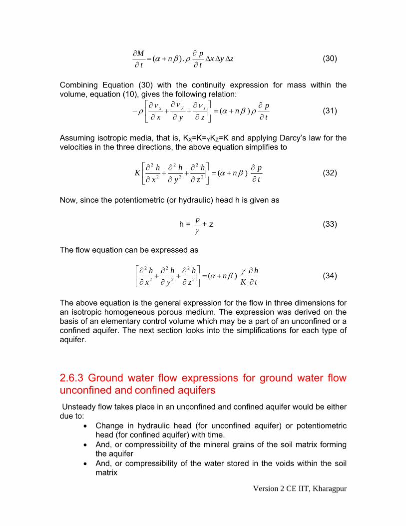
+=∂∂ ρβα .)( (30)

Combining Equation (30) with the continuity expression for mass within the volume, equation (10), gives the following relation:

tp

nzyxzyx

∂∂

+=⎥⎦

⎤⎢⎣

⎡∂

∂+

∂

∂+

∂∂

− ρβαννν

ρ )( (31)

Assuming isotropic media, that is, KX=K=YKZ=K and applying Darcy’s law for the velocities in the three directions, the above equation simplifies to

tp

nzh

yh

xh

K∂∂

+=⎥⎦

⎤⎢⎣

⎡

∂∂

+∂∂

+∂∂

)(2

2

2

2

2

2

βα (32)

Now, since the potentiometric (or hydraulic) head h is given as

h = γp + z (33)

The flow equation can be expressed as

th

Kn

zh

yh

xh

∂∂

+=⎥⎦

⎤⎢⎣

⎡∂∂

+∂∂

+∂∂ γβα )(2

2

2

2

2

2

(34)

The above equation is the general expression for the flow in three dimensions for an isotropic homogeneous porous medium. The expression was derived on the basis of an elementary control volume which may be a part of an unconfined or a confined aquifer. The next section looks into the simplifications for each type of aquifer. 2.6.3 Ground water flow expressions for ground water flow unconfined and confined aquifers Unsteady flow takes place in an unconfined and confined aquifer would be either due to:

• Change in hydraulic head (for unconfined aquifer) or potentiometric head (for confined aquifer) with time.

• And, or compressibility of the mineral grains of the soil matrix forming the aquifer

• And, or compressibility of the water stored in the voids within the soil matrix


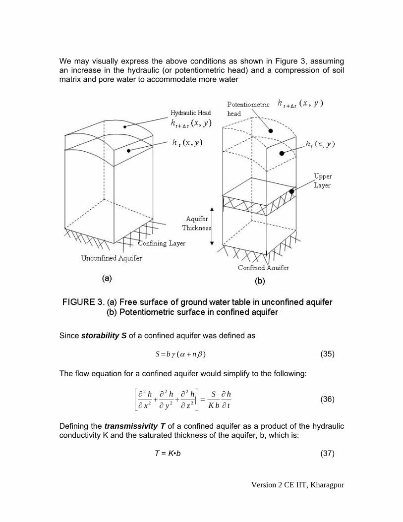
We may visually express the above conditions as shown in Figure 3, assuming an increase in the hydraulic (or potentiometric head) and a compression of soil matrix and pore water to accommodate more water

Since storability S of a confined aquifer was defined as

)( βαγ nbS += (35)

The flow equation for a confined aquifer would simplify to the following:

th

bKS

zh

yh

xh

∂∂

=⎥⎦

⎤⎢⎣

⎡∂∂

+∂∂

+∂∂

2

2

2

2

2

2

(36)

Defining the transmissivity T of a confined aquifer as a product of the hydraulic conductivity K and the saturated thickness of the aquifer, b, which is:

T = K•b (37)


The flow equation further reduces to the following for a confined aquifer

th

TS

zh

yh

xh

∂∂

=⎥⎦

⎤⎢⎣

⎡∂∂

+∂∂

+∂∂

2

2

2

2

2

2

(38)

For unconfined aquifers, the storability S is given by the following expression

S = Sy + h Ss (39)

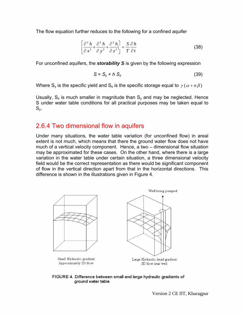
Where Sy is the specific yield and Ss is the specific storage equal to )( βαγ n+ Usually, Ss is much smaller in magnitude than Sy and may be neglected. Hence S under water table conditions for all practical purposes may be taken equal to Sy. 2.6.4 Two dimensional flow in aquifers Under many situations, the water table variation (for unconfined flow) in areal extent is not much, which means that there the ground water flow does not have much of a vertical velocity component. Hence, a two – dimensional flow situation may be approximated for these cases. On the other hand, where there is a large variation in the water table under certain situation, a three dimensional velocity field would be the correct representation as there would be significant component of flow in the vertical direction apart from that in the horizontal directions. This difference is shown in the illustrations given in Figure 4.


In case of two dimensional flow, the equation flow for both unconfined and confined aquifers may be written as,

th

TS

yh

xh

∂∂

=⎥⎦

⎤⎢⎣

⎡∂∂

+∂∂

2

2

2

2

(40)

There is one point to be noted for unconfined aquifers for hydraulic head ( or water table) variations with time. It is that the change in the saturated thickness of the aquifer with time also changes the transmissivity, T, which is a product of hydraulic conductivity K and the saturated thickness h. The general form of the flow equation for two dimensional unconfined flow is known as the Boussinesq equation and is given as

th

KS

yhh

yxhh

xy

∂∂

=⎟⎟⎠

⎞⎜⎜⎝

⎛∂∂

∂∂

+⎟⎟⎠

⎞⎜⎜⎝

⎛∂∂

∂∂

(41)

Where Sy is the specific yield. If the drawdown in the unconfined aquifer is very small compared to the saturated thickness, the variable thickness of the saturated zone, h, can be replaced by an average thickness, b, which is assumed to be constant over the aquifer. For confined aquifer under an unsteady condition though the potentiometric surface declines, the saturated thickness of the aquifer remains constant with time and is equal to an average value ‘b’. Solving the ground water flow equations for flow in aquifers require the help of numerical techniques, except for very simple cases.

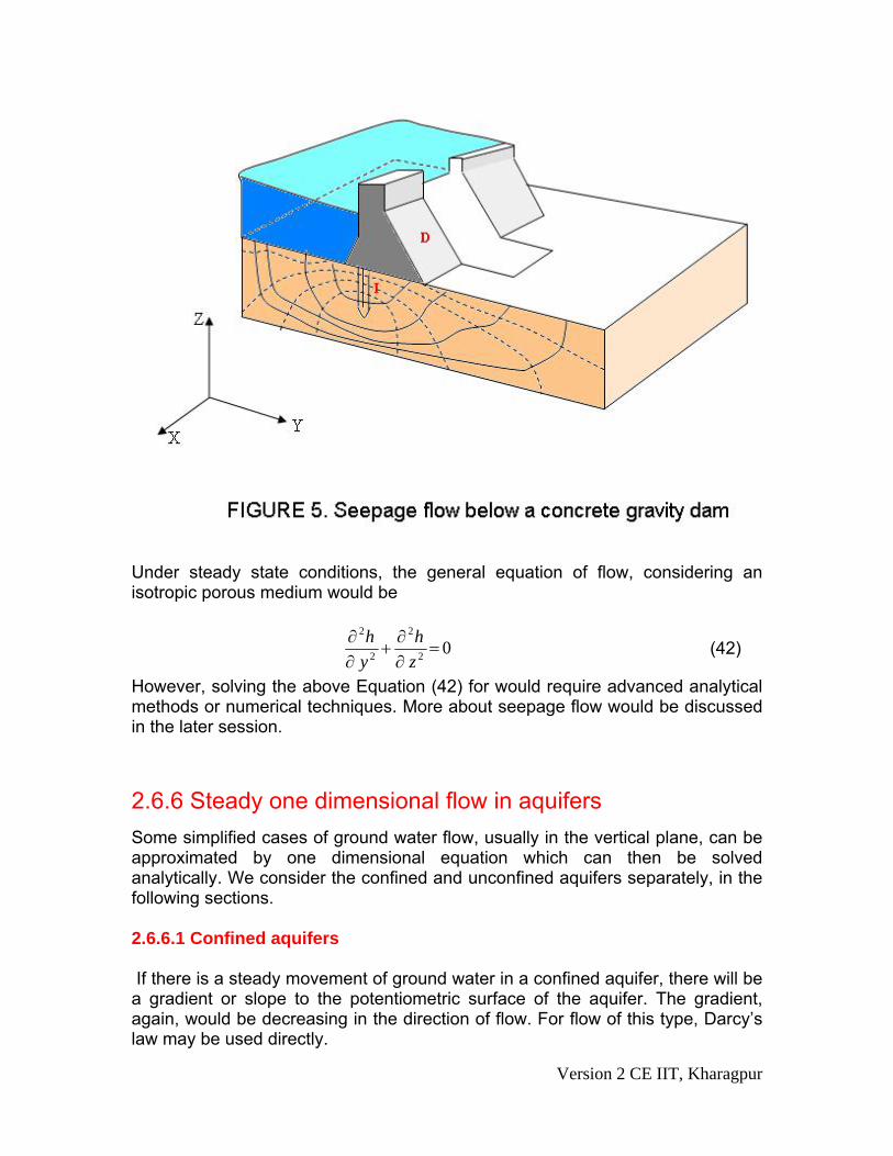
2.6.5 Two dimensional seepage flow In the last section, examples of two dimensional flow were given for aquifers, considering the flow to be occurring, in general, in a horizontal plane. Another example of two dimensional flow would that be when the flow can be approximated. to be taking place in the vertical plane. Such situations might occur as for the seepage taking place below a dam as shown in Figure 5.


Under steady state conditions, the general equation of flow, considering an isotropic porous medium would be

02

2

2

2

=∂∂

+∂∂

zh

yh

(42)

However, solving the above Equation (42) for would require advanced analytical methods or numerical techniques. More about seepage flow would be discussed in the later session.

2.6.6 Steady one dimensional flow in aquifers Some simplified cases of ground water flow, usually in the vertical plane, can be approximated by one dimensional equation which can then be solved analytically. We consider the confined and unconfined aquifers separately, in the following sections. 2.6.6.1 Confined aquifers If there is a steady movement of ground water in a confined aquifer, there will be a gradient or slope to the potentiometric surface of the aquifer. The gradient, again, would be decreasing in the direction of flow. For flow of this type, Darcy’s law may be used directly.


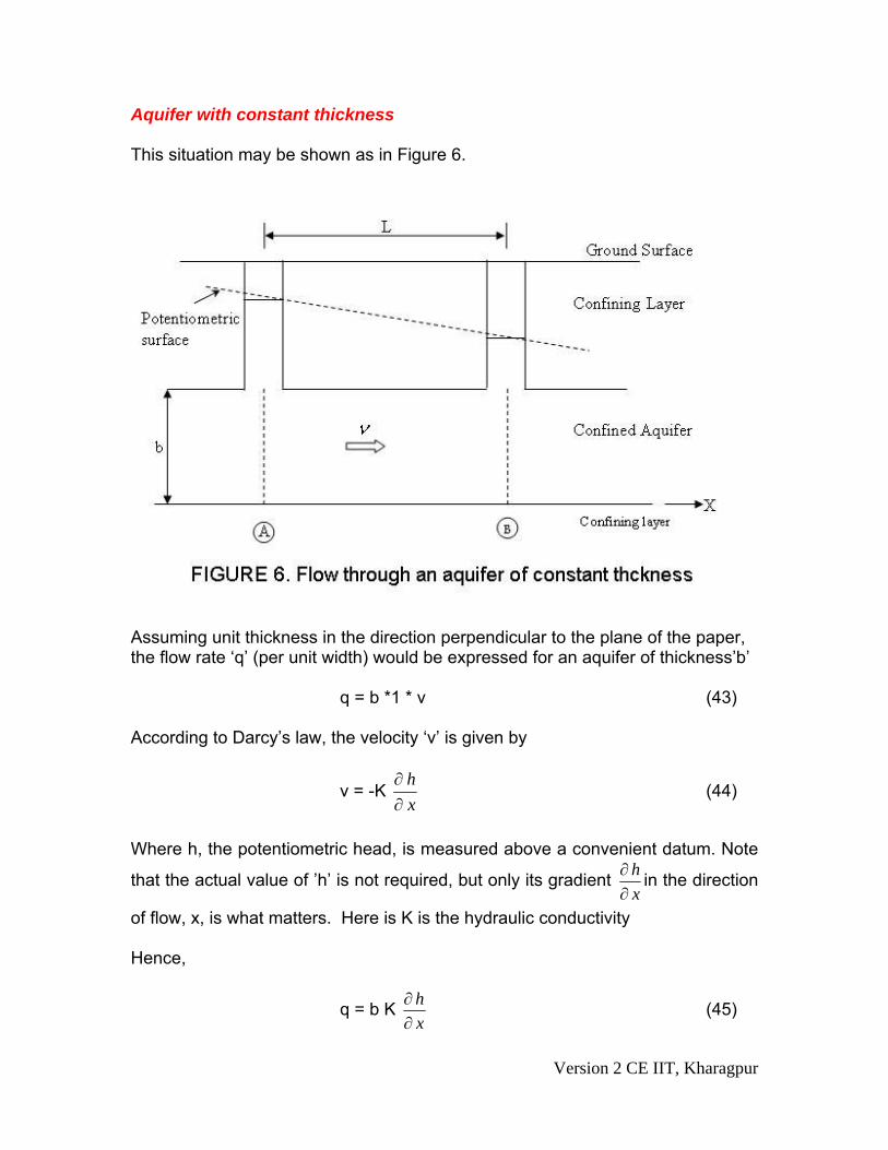
Aquifer with constant thickness This situation may be shown as in Figure 6.

Assuming unit thickness in the direction perpendicular to the plane of the paper, the flow rate ‘q’ (per unit width) would be expressed for an aquifer of thickness’b’

q = b *1 * v (43)

According to Darcy’s law, the velocity ‘v’ is given by

v = -K xh

∂∂

(44)

Where h, the potentiometric head, is measured above a convenient datum. Note

that the actual value of ’h’ is not required, but only its gradient xh

∂∂ in the direction

of flow, x, is what matters. Here is K is the hydraulic conductivity Hence,

q = b K xh

∂∂ (45)


The partial derivative of ‘h’ with respect to ‘x’ may be written as normal derivative since we are assuming no variation of ‘h’ in the direction normal to the paper. Thus

q = - b K xdhd (46)

For steady flow, q should not vary with time, t, or spatial coordinate, x. hence,

02

2

=−=xdhdKb

xdqd

(47)

Since the width, b, and hydraulic conductivity, K, of the aquifer are assumed to be constants, the above equation simplifies to:

02

2

=xdhd (48)

Which may be analytically solved as

h = C1 x + C2 (49)

Selecting the origin of coordinate x at the location of well A (as shown in Figure 6), and having a hydraulic head,hA and also assuming a hydraulic head of well B, located at a distance L from well A in the x-direction and having a hydraulic head hB, we have:

hA = C1.0+C2 and hB = C1.L+C2

Giving

C1 = h - hA /L and C2= hA (50)

Thus the analytical solution for the hydraulic head ‘h’ becomes:

H = AAB hx

Lhh

+−

(51)

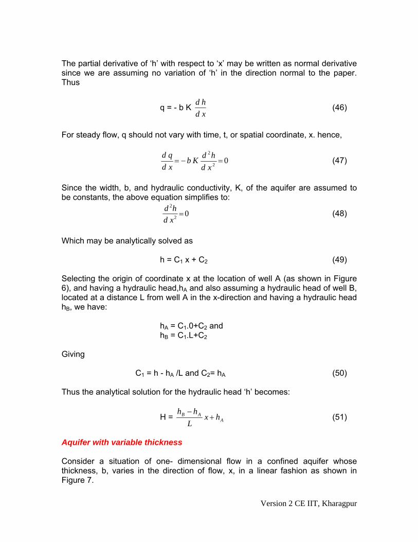
Aquifer with variable thickness Consider a situation of one- dimensional flow in a confined aquifer whose thickness, b, varies in the direction of flow, x, in a linear fashion as shown in Figure 7.


The unit discharge, q, is now given as

q = - b (x) K dxdh (52)

Where K is the hydraulic conductivity and dh/dx is the gradient of the potentiometric surface in the direction of flow,x. For steady flow, we have,

02

2

=⎥⎦

⎤⎢⎣

⎡+−=

xdhdb

dxdh

dxdbK

dxdq

(53)

Which may be simplified, denoting dxdb as b′

02

2

=′+dxdhb

xdhdb (54)

A solution of the above differential equation may be found out which may be substituted for known values of the potentiometric heads hA and hB in the two observation wells A and B respectively in order to find out the constants of integration.


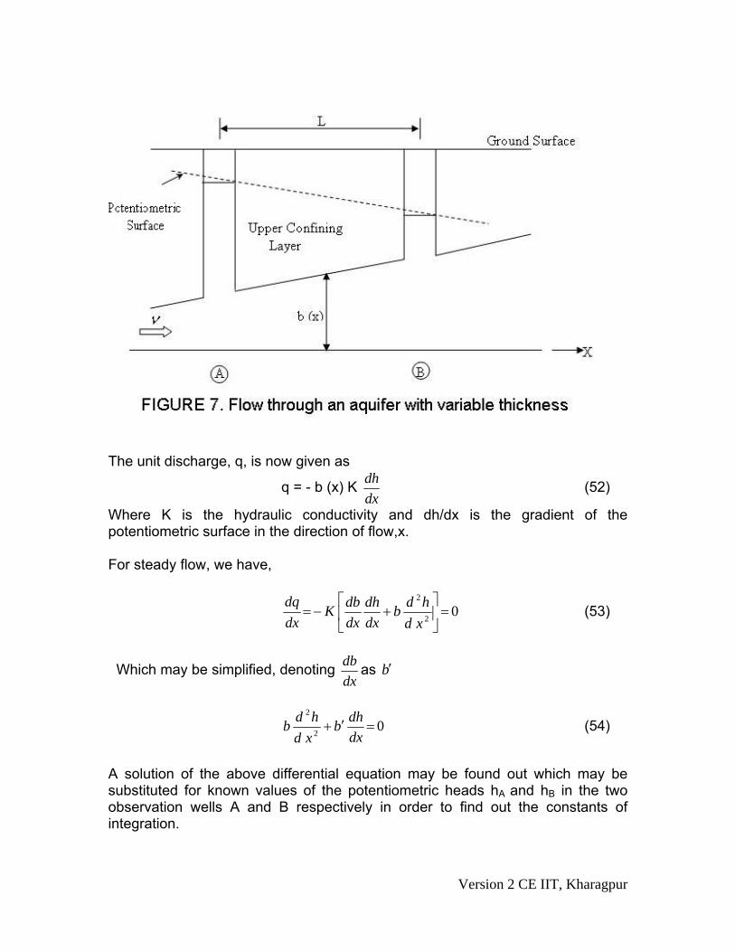
2.6.6.2 Unconfined aquifers In an unconfined aquifer, the saturated flow thickness, h is the same as the hydraulic head at any location, as seen from Figure 8:

Considering no recharge of water from top, the flow takes place in the direction of fall of the hydraulic head, h, which is a function of the coordinate, x taken in the flow direction. The flow velocity, v, would be lesser at location A and higher at B since the saturated flow thickness decreases. Hence v is also a function of x and increases in the direction of flow. Since, v, according to Darcy’s law is shown to be

dxdhK=ν (55)

the gradient of potentiometric surface, dh/dx, would (in proportion to the velocities) be smaller at location A and steeper at location B. Hence the gradient of water table in unconfined flow is not constant, it increases in the direction of flow. This problem was solved by J.Dupuit, a French hydraulician, and published in 1863 and his assumptions for a flow in an unconfined aquifer is used to approximate the flow situation called Dupuit flow. The assumptions made by Dupuit are:

• The hydraulic gradient is equal to the slope of the water table, and


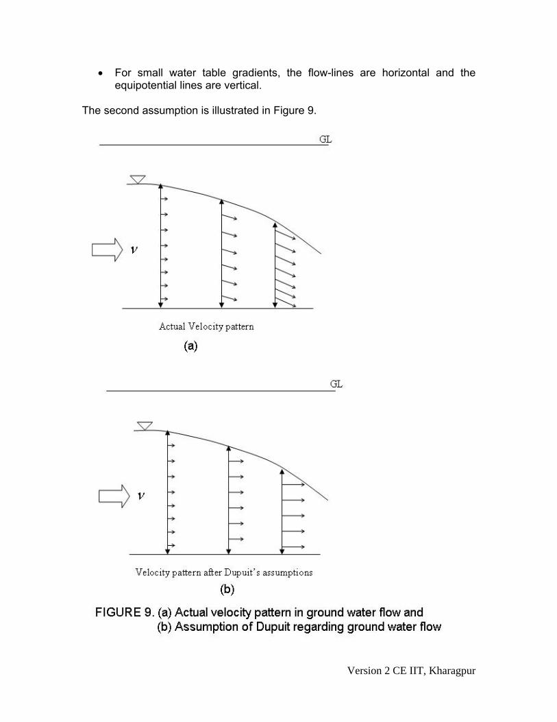
• For small water table gradients, the flow-lines are horizontal and the equipotential lines are vertical.

The second assumption is illustrated in Figure 9.


Solutions based on the Dupuit’s assumptions have proved to be very useful in many practical purposes. However, the Dupuit assumption do not allow for a seepage face above an outflow side. An analytical solution to the flow would be obtained by using the Darcy equation to express the velocity, v, at any point, x, with a corresponding hydraulic

gradientdxdh , as

dxdhK−=ν (56)

Thus, the unit discharge, q, is calculated to be

dxdhhKq −= (57)

Considering the origin of the coordinate x at location A where the hydraulic head us hA and knowing the hydraulic head hB at a location B, situated at a distance L from A, we may integrate the above differential equation as:

∫ ∫−=L h

h

B

A

dhhKdxq0

(58)

Which, on integration, leads to

hB

hA

L hKxq2

.2

0−= (59)

Or,

q . L = K ⎥⎥⎦

⎤

⎢⎢⎣

⎡−

22

22AB hh (60)

Rearrangement of above terms leads to, what is known as the Dupuit equation:

⎥⎥⎦

⎤

⎢⎢⎣

⎡ −−=

Lhh

Kq AB22

21 (61)


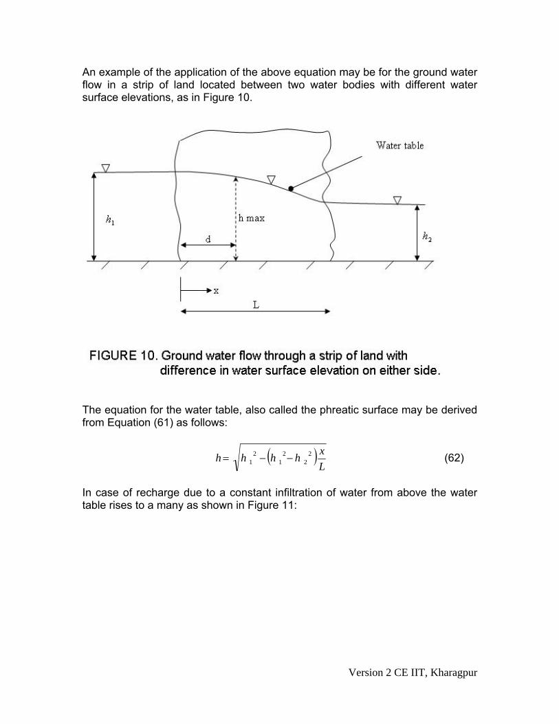
An example of the application of the above equation may be for the ground water flow in a strip of land located between two water bodies with different water surface elevations, as in Figure 10.

The equation for the water table, also called the phreatic surface may be derived from Equation (61) as follows:

( )Lxhhhh 2

22

12

1 −−= (62)

In case of recharge due to a constant infiltration of water from above the water table rises to a many as shown in Figure 11:


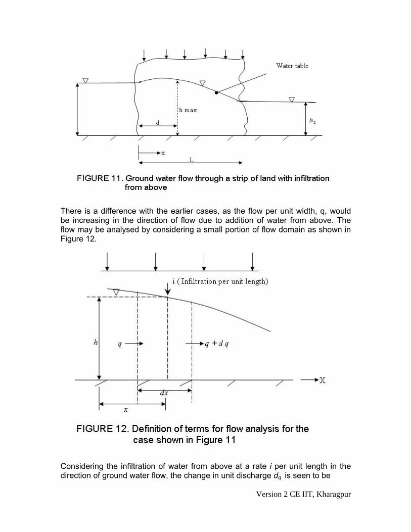
There is a difference with the earlier cases, as the flow per unit width, q, would be increasing in the direction of flow due to addition of water from above. The flow may be analysed by considering a small portion of flow domain as shown in Figure 12.

Considering the infiltration of water from above at a rate i per unit length in the direction of ground water flow, the change in unit discharge dq is seen to be


dq = i .dx (63)

Or,

idxdq

= (64)

From Darcy’s law,

dxhdk

dxdhhKq )(

21..

2

−=−= (65)

( )2

22

21

dxhdK

dxdq

−= (66)

Substituting the expression fordxdq , we have,

idx

hdK =− 2

22 )(21

(67)

Or,

ki

dxhd .2)(2

22

= (68)

The solution for this equation is of the form

2122 2 CxCxKh +=+ (69)

If, now, the boundary condition is applied as, At x = 0, h = h1, and At x = L, h = h2 The equation for the water table would be:

( )xxL

Kix

Lhh

hh )(2

12

121 −+

−−=

(70)

And,


xqqx 20 += (71)

Where is the unit discharge at the left boundary, x = 0, and may be found out to be

0q

( )

22

21

21

0iL

Lhh

q −−

= (72)

Which gives an expression for unit discharge at any point x from the origin as xq

( )⎟⎠⎞

⎜⎝⎛ −−

−= xLi

LhhKqx 22

21

21 (73)

For no recharge due to infiltration, i = 0 and the expression for is then seen to become independent of x, hence constant, which is expected.

xq

References Raghunath, H M (2002) Ground Water (Second Edition), New Age International Pvt. Ltd.


Documents

Principles of Ground water flow - IITs and IISc elearning Courses