527

PRINCIPLES OF MEDICAL STATISTICS

IX—FURTHER EXAMPLES AND

DISCUSSION OF Х2THE y2 test has a wide applicability and forms

a useful test of " significance " in many medicalstatistical problems, especially those in which theobservations must be grouped in descriptive cate-

gories (as in the state of nutrition) and are not capableof being expressed quantitatively ; some furtherexamples of its use may, therefore, be supplied.

A TEST OF DIFFERENCES BETWEEN SERA

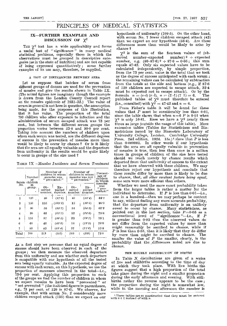
Let us suppose that batches of serum fromdifferent groups of donors are used for the preventionof measles and give the results shown in Table IX.(The actual figures are imaginary though the exampleis drawn from the London County Council reporton the measles epidemic of 1931-32.) The value ofserum in general is not here in question, the assumptionbeing made, for the purposes of this illustration,that it has value. The proportion of the total700 children who after exposure to infection and theadministration of serum escaped attack was 73 percent., but between the different serum groups the

proportion varies between 53-8 and 90-0 per cent.

Taking into account the numbers of children uponwhom each serum was tested, are the different degreesof success in the prevention of measles more thanwould be likely to occur by chance ? Or is it likelythat the sera are all equally valuable and the departurefrom uniformity in the results would be quite likelyto occur in groups of the size used ?

TABLE IX-111easles Incidence and Serum Treatment

As a first step we presume that an equal degree ofsuccess should have been observed in each of the

groups; we then measure the observed departurefrom this uniformity and see whether such departureis compatible with our hypothesis of all the testedsera being equally valuable. As the expected degree ofsuccess with each serum, on this hypothesis, we use theproportion of successes observed in the total-i.e.,73-0 per cent. Applying this proportion to eachof the groups we find the number of children in whomwe expect measles to have been " prevented " or" not prevented " (the italicised figures in parentheses,e.g., 73 per cent. of 120 is 87-6). We observe, forexample, that with serum No. 2 considerably morechildren escaped attack (135) than we expect on our

hypothesis of uniformity (109-5). On the other hand,with serum No. 7 fewer children escaped attack (43)than we expect on our hypothesis (58-4). Are thesedifferences more than would be likely to arise bychance ?

X2 is the sum of the fourteen values of (ob-served number-expected number) 2 — expectednumber, e.g. (80-87-6) 2 - 87-6 = 0-66; this sum

equals 47-42. Only six expected values have to becalculated independently, by simple proportion,from the 73 per cent. value in the total that we tookas the degree of success anticipated with each serum ;the remaining values can be calculated by subtractionfrom the totals at the side and bottom (e.g., if 87’6of 120 children are expected to escape attack, 32-4must be expected not to escape attack). Or by theformula n = (c-l) (r-l), n = (2-1) (7-1) = 6. The

published tables of X2 must therefore be entered

(i.e., consulted) with X2 = 47.42 and n = 6.From Fisher’s table it will be found for these

values that P must be considerably less than 0.01,since the table shows that when n=6 Pis 0.01 when

X2 is only 16-81. Here we have a X2 nearly threetimes as large (outside the range of this table). Moreextensive tables (Tables for Statisticians and Bio-metricians issued by the Biometric Laboratory of

University College, London. Cambridge UniversityPress. 2nd edition. 1924. 15s.) show that P is lessthan 0.000001. In other words if our hypothesisthat the sera are all equally valuable in preventionof measles is true, then less than once in a milliontimes in groups of children of the size here testedshould we reach merely by chance results whichdeparted from that uniformity of success to the extentthat we have observed with these children. We maytherefore reject our hypothesis and conclude thatthese results differ by more than is likely to be dueto cnance, tnat, all otner revelant factors Dmng equal,some sera were more efficient than others.Whether we need the more exact probability taken

from the larger tables is rather a matter for theindividual to determine. If P is less than 0-01-i.e.,one in a hundred-then we may perhaps be contentto say, without finding any more accurate probability,that the departure from uniformity is an unlikelyevent to occur by chance. Many statisticians, as

pointed out in the last section, take P=005 as aconventional level of "significance "-i.e.; if Pis greater than 0-05 then the observed values donot differ from the expected values by more thanmight reasonably be ascribed to chance, while ifP is less than 0.05, then it is likely that they do differby more than might be ascribed to chance. Thesmaller the value of P the smaller, clearly, is the

probability that the differences noted are due tochance.

THE HOURLY DISTRIBUTION OF BIRTHS

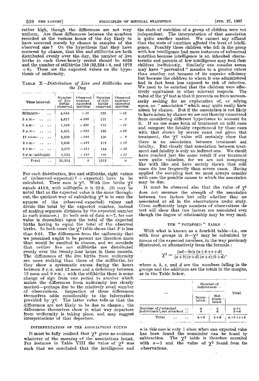
In Table X distributions are given of a seriesof live and stillbirths according to the time of dayat which they took place. With live births thefigures suggest that a high proportion of the totaltake place during the night and a smaller proportionduring the early afternoon and evening. With still-births rather the reverse appears to be the case ;the proportion during the night is somewhat low,while in the morning and afternoon the number is

1 These tables are so constructed that they must be enteredwith n+ 1 instead of with n.

528

rather high, though the differences are not veryuniform. Are these differences between the numbersrecorded at the various hours of the day likely tohave occurred merely by chance in samples of theobserved size ? On the hypothesis that they haveoccurred by chance, that live and stillbirths are bothdistributed evenly over the day, the number of livebirths in each three-hourly period should be 4028and the number of stillbirths 159 (32,224—8, and 1272—8). These are the expected values on the hypo-thesis of uniformity.

TABLE X-Distribution of Live and Stillbirths overthe Day

For each distribution, live and stillbirths, eight valuesof ((observed-expected) 2 expected) have to becalculated. Their sum is or2. With live births X2equals 413,0, with stillbirths it is 23-8. (It may benoted that as the expected value is the same through-out, the quickest way of calculating X2 is to sum thesquares of the (observed-expected) values anddivide this total by the expected number, insteadof making separate divisions by the expected numberin each instance.) In both sets of data n=7, for onevalue is dependent upon the total of the expectedbirths having to equal the total of the observedbirths. In both cases the X2 table shows that P is lessthan 0-01. The differences from the uniformity thatwe presumed ought to be present are therefore morethan would be ascribed to chance, and we concludethat neither live nor stillbirths are distributed

evenly over the twenty-four hours in these records.The differences of the live births from uniformityare more striking than those of the stillbirths, forthey show a systematic excess during the hoursbetween 9 P.M. and 12 noon and a deficiency between12 noon and 9 P.M. ; with the stillbirths there is some

change of sign from one period to another whichmakes the differences from uniformity less clearlymarked-perhaps due to the relatively small numberof observations. Inspection of these differencesthemselves adds considerably to the informationprovided by X2. The latter value tells us that thedifferences are not likely to be due to chance ; thedifferences themselves show in what way departurefrom uniformity is taking place, and may suggestinterpretations of that departure.

INTERPRETATION OF THE ASSOCIATIONS FOUND

It must be fully realised that Z2 gives no evidencewhatever of the meaning of the associations found.For instance in Table VIII the value of X2 wassuch that we concluded that the intelligence and

the state of nutrition of a group of children were notindependent. The interpretation of that associationis quite another matter. We cannot say offhandthat the state of nutrition affected the level of intelli.gence. Possibly those children who fell in the groupwith low intelligence had more instances of subnormalnutrition because intelligence is an inherited charac-teristic and parents of low intelligence may feed theirchildren inefficiently. Similarly one measles serummay have " prevented " measles to a greater extentthan another not because of its superior efficiencybut because the children to whom it was administeredhad in fact been less exposed to risk of infection.We need to be satisfied that the children were effec-tively equivalent in other relevant respects. Thevalue of the X2 test is that it prevents us from unneces-sarily seeking for an explanation of, or relyingupon, an

" association " which may quite easily havearisen by chance. But if the association is not likelyto have arisen by chance we are not thereby exoneratedfrom considering different hypotheses to account forit. If we use some form of treatment on mild casesand compare the fatality experienced by those caseswith that shown by severe cases not given thattreatment, the X2 value will certainly show thatthere is an association between treatment andfatality. But clearly that association between treat-ment and fatality is only an indirect one. We shouldhave reached just the same result if our treatmentwere quite valueless, for we are not comparinglike with like and have merely shown that mildcases die less frequently than severe cases. Havingapplied the sampling test we must always considerwith care the possible causes to which the associationmay be due.

It must be observed also that the value of X2does not measure the strength of the associationbetween two factors but only whether they are

associated at all in the observations under study.Given sufficiently large numbers of observations thetest will show that two factors are associated even

though the degree of relationship may be very small.

THE " FOURFOLD " TABLE’

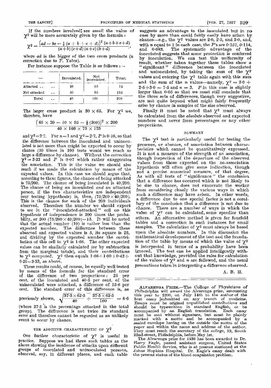
With what is known as a fourfold table-i.e., onewith four groups in it—y2 may be calculated bymeans of the expected numbers, in the way previouslyillustrated, or alternatively from the formula :

where a, b, c, and d are the numbers falling in thegroups and the additions are the totals in the margins,as in the Table below.

n in this case is only 1 since when one expected valuehas been found the remainder can be found bysubtraction. The X2 table is therefore consultedwith n = 1 and the value of X2 found from theobservations.

529

If the numbers involved are small the value of

X2 will be more accurately given by the formula :

x2 = (ad - be - i (a + b + e + d))2 (a+b+e+d) ,)IX (a+b) (e+d) (a+e) (b+d) ’

where ad is the bigger of the two cross products (acorrection due to F. Yates).

For instance suppose the Table is as follows :-

The larger cross product is 30 x 65. For X2 we,therefore, have

z 65 x 30 - 10 x 95 - i- (200)) X 20040 X 160 X 75 x 125

and x2=27. For n=l and X2=2.7, Pis 010, so thatthe difference between the inoculated and uninocu-lated is not more than might be expected to occur bychance (10 times in 100 tests would we reach so

large a difference by chance). Without the correction

X2 = 3,33 and P is 0-07 which rather exaggeratesthe association. This is the value we should alsoreach if we made the calculation by means of theexpected values. In this case we should argue that,according to these figures, the chance of being attackedis 75/200. The chance of being inoculated is 40/200.The chance of being an inoculated and an attackedperson, if the two characteristics are independent(our testing hypothesis) is, then, (75/200 X 40/200).This is the chance for each of the 200 individualsobserved. Therefore the number we should expectto see in the " inoculated-attacked " cell on thishypothesis of independence is 200 times the proba-bility, or 200 (75/200 X 40/200)=15. It will be notedthat the actual number (10) is rather less than the

expected number. The difference between theseobserved and expected values is 5, its square is 25,and dividing by the expected number the contri-bution of this cell to y2 is 1.66. The other expectedvalues can be similarly calculated (or by subtractionfrom the marginal totals), and their contributionsto X2 computed. X2 then equals 1-66+1-00+0-42+0.25=3.33, as above.These results could, of course, be equally well tested

by means of the formula for the standard error

of the difference of two proportions : 25 percent. of the inoculated and 40-6 per cent. of theuninoculated were attacked, a difference of 15.6 percent. The standard error of this difference is, as

previously shown, = 8.6

(where 37.5 is the percentage attacked in the totalgroup). The difference is not twice its standarderror and therefore cannot be regarded as an unlikelyevent to occur by chance.

THE ADDITIVE CHARACTERISTIC OF X2One further characteristic of X2 is useful in

practice. Suppose we had three such tables as theabove showing the incidence of attacks upon differentgroups of inoculated and uninoculated persons,observed, say, in different places, and each table 1

! suggests an advantage to the inoculated but in nocase by more than could fairly easily have arisen bychance-e.g., the X2 values are 2-0, 2,5, and 3.0, and,with n equal to 1 in each case, the P’s are 0-157, 0-114,and 0-083. The systematic advantage of theinoculated suggests that some protection is conferredby inoculation. We can test this uniformity of

result, whether taken together these tables show a"

significant " difference between the inoculatedand uninoculated, by taking the sum of the x2values and entering the X2 table again with this sumand the sum of the n values-namely, X2 = 2-0 +2-5+3-0 = 7-5 and n = 3. P in this case is slightlylarger than 0-05 so that we must still conclude thatthe three sets of differences, though very suggestive,are not quite beyond what might fairly frequentlyarise by chance in samples of the size observed.

Finally it must be noted that X2 must alwaysbe calculated from the absolute observed and expectednumbers and never from percentages or any otherproportions.

SUMMARY

The &khgr;2 test is particularly useful for testing thepresence, or absence, of association between charac-teristics which cannot be quantitatively expressed.It is not a measure of the strength of an association,though inspection of the departure of the observedvalues from those expected on the no-association

hypothesis will often give some indication, thoughnot a precise numerical measure, of that degree.As with all tests of " significance " the conclusionthat a difference has occurred which is not likely tobe due to chance, does not exonerate the workerfrom considering closely the various ways in whichsuch a difference may have arisen. In other words,a difference due to one special factor is not a corol-larv of the conclusion that a difference is not due tochance. There are a number of ways in which thevalue of y2 can be calculated, some speedier thanothers. An alternative method is given for fourfoldtables and a correction in such instances for smallsamples. The calculation of X2 must always be basedupon the absolute numbers. In this discussion themathematical development of the test and the founda-tion of the table by means of which the value of &khgr;2is interpreted in terms of a probability have beenignored. The test can be applied intelligently with-out that knowledge, provided the rules for calculationof the values of &khgr;2 and n are followed, and the usualprecautions taken in interpreting a difference observed.

A. B. H.

ALVARENGA PRIZE.—The College of Physicians ofPhiladelphia will award the Alvarenga prize, amountingthis year to$200, on July 14th to the author of thebest essay [submitted on any branch of medicine.Essays must be original unpublished contributions andshould be typewritten in standard English, or be

accompanied by an English translation. Each essaymust be sent without signature, but must be plainlymarked with a motto and be accompanied by a

sealed envelope having on the outside the motto of thepaper and within the name and address of the author.They must reach the secretary of the college, 19, South22nd-street, Philadelphia, before May 1st.The Alvarenga prize for 1936 has been awarded to Dr.

Harry Eagle, passed assistant surgeon, United StatesPublic Health Service, who is at present stationed at theJohns Hopkins Hospital. Dr. Eagle’s essay dealt withthe present status of the blood coagulation problem.