Embed Size (px)
Citation preview

M. Lustig, EECS UC Berkeley
Principles of MRIEE225E / BIO265
Lecture 19
Instructor: Miki LustigUC Berkeley, EECS
1
M. Lustig, EECS UC Berkeley
Name That Artifact
http://mri-info.net2
M. Lustig, EECS UC Berkeley
RF Interference During Readout
readout
1D FFT
3
M. Lustig, EECS UC Berkeley
RF Interference During Readout
readout
1D FFT
1D FFT
4

M. Lustig, EECS UC Berkeley
Name That Artifact
http://mri-info.net
• Which direction is readout?
• How can you find frequency of RF?
5
M. Lustig, EECS UC Berkeley
Off -Resonance Effects on Imaging
x
0 = x+!
E
(~r)
�G
x
phase/dephasing displacement
An on-resonance spin at position:
Produces the same signal as a spin at x, with off-resonance!
mxy
(~r, t) = mxy
(~r, 0)e�i!
E
(~r)TEe�i2⇡k
x
(t)⇣x+
!
E
(~r)�G
x
⌘
d~r
6
M. Lustig, EECS UC Berkeley
Examples:
shape
signal loss
readout direction?
7
M. Lustig, EECS UC Berkeley
Examples: Phase vs Echo Timewater and fat are “in phase” “ out of phase”
Fat on Gradient Echo Images
water and lipids in phase water and lipids out-of-phase
8

M. Lustig, EECS UC Berkeley
Example: Chemical Shift
x
0 = x+!
E
(~r)
�G
x
Increasing Gx reduces chemical shift artifact
9
�
2⇡G
x
= 1
E(~r) = 3
!E(~r) = 2⇡ · 200
�x = x
0 � x =!
E
(~r)
�G
x
=��2⇡ · 200 Hz
��2⇡ · 1 KHz/cm= 0.2cm
�x
= 1 mm
M. Lustig, EECS UC Berkeley
Example:
Let,
KHz/cm
ppm
Hz (@1.5T)
At: this is a shift of two pixels!
10
2 cyc
220 Hz⇡ 9.1 ms
M. Lustig, EECS UC Berkeley
Effects in Spin-Warp
• Off-Resonance–Modest spatial distortions ( few pixels)–Relatively benign artifacts–Reduce artifacts with large Gx
• Chemical-Shift– Fat shift of -220Hz @ 1.5T, -440Hz @ 1.5T– Fat image is displaced from Water– In practice F/W shift limited to ~2pixels (4pix @3T) 2 pixels shift are two cycles of linear phase across k-space
11
M. Lustig, EECS UC Berkeley
Off-Resonance in EPI
point-spread function
Example: Lipids
phase accumulation
1ms ⇒ 0.44cyc
0.44cyc ⇐ 1ms
1ms ⇒ 0.44cyc
0.44cyc ⇐ 1ms 96ms ⇒
42.24cyc
12

M. Lustig, EECS UC Berkeley
Off-Resonance in EPI
point-spread function simulation Leg
13
M. Lustig, EECS UC Berkeley
Off-Resonance in Spiralpoint-spread functionphase accumulation
2 ms ⇒ 0.88cyc
realimag
14
M. Lustig, EECS UC Berkeley
Off-Resonance in SpiralReadout time @3T:
2ms 5ms 13ms
Spiral scanwith linear off-resonance
15
M. Lustig, EECS UC Berkeley
Echoes
• Early in NMR people noticed the following odd behavior (Hann, 1950)
Two 90° excitations, separated by T cause large signal to form at 2T, Why?
16

0� 0+ ⌧+⌧� 2⌧
M. Lustig, EECS UC Berkeley
Spin Echo Pulse Sequence
RF
90180
T2* ?
17
M. Lustig, EECS UC Berkeley
Spin Echo Pulse Sequence
RF
90180
T2
T2*
T2*
Any signal loss due to dephasingis recovered at the spin-echo
If wE(r,t) changes over time, refocusing is not perfect
Provides probe to measure molecular motion
18
M. Lustig, EECS UC Berkeley
Multi-Spin Echo - CPMG
19
M. Lustig, EECS UC Berkeley
Non uniform dephasing
• Any signal due to dephasing ωE(r)t is refocussed• If ωE(r,t) refocussing not perfect
T2* Huge!but, constant dephasing
time-varyingdephasingshows as T2
20

M. Lustig, EECS UC Berkeley
Large vessels
small vessels
T2(T)
T T T
21
M. Lustig, EECS UC Berkeley
Low Flip Angle Spin Echoes
• Any pulse can produce a spin-echo– 180 maximally refocuses magnetization– Lower refocusing power with lower flip angle– 90 refocusses 1/2 (see homework)
180 90
22
M. Lustig, EECS UC Berkeley
Low Flip Angle Spin Echoes
• Refocusing RF result can be decomposed to several components:– Pass through– Refocused– Parasitic excitation– Magnetization stored in Mz
23
Mxy
= A1 cos(2!E
⌧) +A2 sin(2!E
⌧)| {z }+B1 cos2(!
E
⌧) +B2 sin2(!
E
⌧)| {z }+C1 cos(!E
⌧) + C2 sin(!E
⌧)| {z }
M = Rz
(!E
⌧)Rx
(↵)Rz
(!E
⌧)Rx
(↵)M0
Mxy
=1
2sin(!
E
2⌧)M0 � i sin2(!E
⌧)M0
M. Lustig, EECS UC Berkeley
Low Flip Angle Spin Echoesα
⌧ ⌧
α
passthrough refocused parasitic
For 90 degrees:
In general.... I think
24

M. Lustig, EECS UC Berkeley
Phase Graphs
• Useful to find echo formations
passthrough
refocused
parasitic excitation
longitudinal magn.
echo
αα
25
M. Lustig, EECS UC Berkeley
Phase Graphs
Time�t
Phase !
Mtrans - deph
Mtrans - ref
Mlong
Flip Angle "
Figure 1: Phase graph showing the splitting of
transverse magnetization into 3 parts
by an RF-pulse.
form a spin echo (’180◦-pulse’).
3. A part �
M
long
of the magnetization is convertedto z-magnetization, which is modulated alongω and which can be retrieved by a later α-pulse to form a stimulated echo with amplitude0.5 sin2(α/2).
Such a phase graph is very practical to predict thetime points of echo formation after a series of non-equidistant pulses. For a CPMG-sequence (or otherpulse sequences with regular pulse spacing [7]) it hasalso been used to calculate the signal amplitudesby superposition of all different refocusing pathwaysleading to echo formation. This approach to calculatethe echo amplitude by a sum over all pathways hasbeen called the partition method [7]. The number ofrefocusing pathways increases extremely rapidly withthe echo number: After the N
th pulse 3N−1 echo for-mation pathways occur [9], as demonstrated in Fig. 2.Analytical solutions based on the partition methodhave been published only up to the fourth echo [8].The calculation of echo amplitudes for typical echotrain lengths used in RARE sequences is feasible bycomputers, however, rather unhandy.
! !!
t
Figure 2: Repetitive splitting of the phase graph
as shown in Fig. 1 and described in
the text. In total 3n−1 echo formation
pathways occur.
1.3 Extended Phase Graphs
!"#
t
F ,Z3 3
F-3
F ,Z5 5
F ,Z7 7
F ,Z1 1
F-5
F-1
F-7
$% $&$' $(
Figure 3: EPG for a CPMG experiment. Com-
pared to a conventional phase graph
(Fig. 1), the EPG is not only used to
track the phase of a single magnetiza-
tion vector �
M , but to define new states
F and Z representing spin states of in-
creasing dephasing.
The extended phase graph (EPG) - algorithm [9,10]was devised to create a mathematical framework,by which the ease of qualitative insight into therefocusing pathways offered by the phase graph istransformed into a straightforward algorithm for
3
* from document by Matthias Weigel
26
M. Lustig, EECS UC Berkeley
Extended Phase Graphs
• Each component has different magnitude and phase
• Echo consist of contribution from many pathways
• Can track to calculate magnitude & Phase of echo (Beyond scope... see document by Matthias Weigel)
27
M. Lustig, EECS UC Berkeley
Spin Echo Imaging
• Spin echo negates phase -- Conjugation• How to incorporate in pulse sequence?
Mxy
(~r, t) = Mxy
(~r, 0)e�i2⇡(kx
(t)x+k
y
(t)y)
28

M. Lustig, EECS UC Berkeley
Spin Echo Imaging
• Spin echo negates phase -- Conjugation• How to incorporate in pulse sequence?
29
M. Lustig, EECS UC Berkeley
30
M. Lustig, EECS UC Berkeley
31
M. Lustig, EECS UC Berkeley
imperfect 180 causes parasiticwhich is not phase encoded (HW)
32

M. Lustig, EECS UC Berkeley
33
M. Lustig, EECS UC Berkeley
34
M. Lustig, EECS UC Berkeley
35
M. Lustig, EECS UC Berkeley
what’s the phase graph for all pathways?
36

M. Lustig, EECS UC Berkeley
Fast/Turbo Spin-Echo (RARE)
Hennig ’86figure from Bernstein, King and Zhou
37
M. Lustig, EECS UC Berkeley
Other non-idealities
• RF Inhomogeneity–Affects Excitation
• Spatially varying flip-angle• Spatially varying phase• Can cause problem for fat saturation
–Worse @ high field (wave effects)
–Affects receive
38
M. Lustig, EECS UC Berkeley
RF excitation inhomogeneity
39
M. Lustig, EECS UC Berkeley
40

M. Lustig, EECS UC Berkeley
More later!
41
M. Lustig, EECS UC Berkeley
Gradient non-idealities
42
M. Lustig, EECS UC Berkeley
Concomitant Gradient (Maxwell Terms)
43
M. Lustig, EECS UC Berkeley
Concomitant Gradient (Maxwell Terms)
44
M. Lustig, EECS UC Berkeley
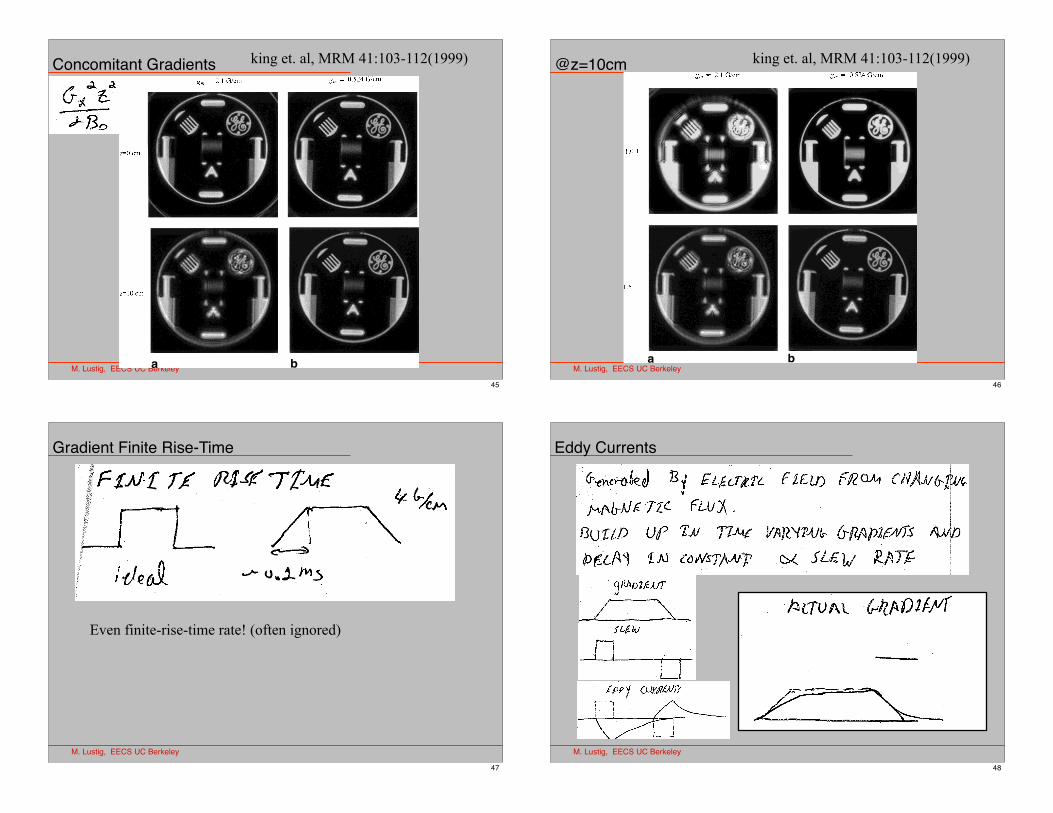
Concomitant Gradients
a b
FIG. 3. Sagittal spiral scans acquiredat isocenter (x ! 0) with (a) gm ! 2.18G/cm, and (b) gm ! 1.11 G/cm, usingfield strength B0 ! 1.5 T. Scan pre-scriptions are (a) 8 interleaves, 4096readout points, "125 kHz bandwidth,4 NEX; and (b) 16 interleaves, 2048readout points, "64 kHz bandwidth, 2NEX. Both (a) and (b) use spin echo,27-cm field of view, TE ! 15, TR !2000, 1-cm thick slice. Spatial resolu-tion, SNR, and off-resonance blurringare approximately the same for bothcases. Arrows show areas of blurringdifferences.
a b
FIG. 2. Axial spiral scans acquired atslice locations z ! 0 and z ! 10 cmwith (a) gm ! 2.1 G/cm, and (b) gm !0.524 G/cm, using field strength B0 !1.5 T. Scan prescriptions are (a) 8interleaves, 4096 readout points,"62.5 kHz bandwidth, 4 NEX; and(b) 32 interleaves, 1024 readoutpoints, "16 kHz bandwidth, 1 NEX.Both (a) and (b) use spin echo, 14-cmfield of view, TE ! 15, TR ! 2000,1-cm slice. Spatial resolution, SNR,and off-resonance blurring are ap-proximately the same for all cases.
Concomitant Gradient Fields in Spiral Scans 105king et. al, MRM 41:103-112(1999)
45
M. Lustig, EECS UC Berkeley
@z=10cm
of known deblurring methods. For the general obliquecase, both through-plane and in-plane effects are present.
Through-Plane Blurring CorrectionFor the axial scan case, for example, Eqs. [2] and [3] give
!c (z, t ) "#z 2
2B0!
0
tg 0
2 dt ! [9]
where t! " 0 at the beginning of the readout during eachinterleave. The phase shift of Eq. [9] is integrated over theexcited magnetization density M(x, y, z) resulting in areceived signal S(t) given by
S (t ) " ! M(x, y, z)e i2$(kxx%kyy)e i!c(z,t) dx dy dz [10]
In Eq. [10], other resonance offsets as well as relaxationeffects are ignored. For 2D imaging, the quadratic phasedispersion across the slice shown in Eq. [9] results in asignal loss. We have not been able to detect a signal losswith slice thickness less than 1 cm, slice offset less than 10cm, and gm & 2.2 G/cm. Therefore the z spatial dependenceof !c in the integral of Eq. [10] can be ignored, and thereceived signal is approximately given by
S (t ) " e i!c(zc, t) ! M (x, y, z)e i2$(kxx%kyy) dx dy dz [11]
where zc is the location of the center of the slice. The phaseshift in Eq. [11] is equivalent to a time-dependent receivefrequency shift of
f (zc, t ) "#
2$
zc2
2B0g 0
2 (t ) [12]
Substituting zc " 10 cm, B0 " 1.5 T, and g0 " 2.2 G/cm inEq. [12] yields f " 69 Hz. For spiral scans, frequency shiftssmaller than 69 Hz cause noticable blurring (25).
The following two methods can be used to remove theeffect of !c(zc, t). First, the receive frequency can bedynamically shifted by f(zc, t) during data acquisition. As aspecial case of this approach, on high slew rate systems,the gradient amplitude is approximately constant for mostof the readout, i.e., g0(t) " gm. For such systems, a goodcorrection (not shown) is obtained by using a time-independent receive frequency shift fc(zc) during dataacquisition given by
fc (zc ) "#
2$
zc2
2B0gm
2 [13]
Second, the data can be demodulated during reconstruc-tion. Spiral scans are normally reconstructed using grid-ding (33, 34). Demodulation before gridding can be per-formed by multiplying the time domain data by the factor
a b
FIG. 4. Axial spiral scans acquired atz" 10 cmwith (a) gm " 2.1 G/cm, and(b) gm " 0.524 G/cm using fieldstrengths B0 " 1.0 T and B0 " 1.5 T.Scan prescriptions are the same asshown in Fig. 2.
106 King et al.king et. al, MRM 41:103-112(1999)
46
M. Lustig, EECS UC Berkeley
Gradient Finite Rise-Time
Even finite-rise-time rate! (often ignored)
47
M. Lustig, EECS UC Berkeley
Eddy Currents
48

M. Lustig, EECS UC Berkeley
49
M. Lustig, EECS UC Berkeley
Eddy Currents
50
M. Lustig, EECS UC Berkeley
Pre-emphasis
51