Privacy-Preserving Deep Learning via Additively HomomorphicEncryption?

Le Trieu Phong1, Yoshinori Aono1, Takuya Hayashi1,2, Lihua Wang1, and Shiho Moriai1

1 National Institute of Information and Communications Technology (NICT), Japan2 Kobe University, Japan

{phong, aono, wlh, shiho.moriai}@nict.go.jpt-hayashi@eedept.kobe-u.ac.jp

Abstract. We build a privacy-preserving deep learning system in which many learning participantsperform neural network-based deep learning over a combined dataset of all, without actually revealingthe participants’ local data to a central server. To that end, we revisit the previous work by Shokriand Shmatikov (ACM CCS 2015) and point out that local data information may be actually leaked toan honest-but-curious server. We then move on to fix that problem via building an enhanced systemwith following properties: (1) no information is leaked to the server; and (2) accuracy is kept intact,compared to that of the ordinary deep learning system also over the combined dataset.

Our system is a bridge between deep learning and cryptography: we utilise asynchronous stochasticgradient descent applied to neural networks, in combination with additively homomorphic encryption.We show that our usage of encryption adds tolerable overhead to the ordinary deep learning system.

keywords: Privacy, deep learning, neural network, additively homomorphic encryption, LWE-basedencryption, Paillier encryption.

1 Introduction

1.1 Background

In recent years, deep learning (aka, deep machine learning) has produced exciting results in bothacamedia and industry, in which deep learning systems are approaching or even surpassing human-level accuracy. This is thanks to algorithmic breakthroughs and physical parallel hardware appliedto neural networks when processing massive amount of data.

Massive collection of data, while vital for deep learning, raises the issue of privacy. Individually,a collected photo can be permanently kept on a server of a company, out of the control of the photo’sowner. At law, privacy and confidentiality worries may prevent hospitals and research centers fromsharing their medical datasets, baring them from enjoying the advantage of large-scale deep learningover the joint datasets.

As a directly related work, Shokri and Shmatikov (ACM CCS 2015) [26] presented a system forprivacy-preserving deep learning, allowing local datasets of several participants staying home whilethe learned model for the neural network over the joint dataset can be obtained by the participants.To achieve the result, the system in [26] needs the following: each learning participant, using localdata, first computes gradients of a neural network; then a part (e.g. 1% ∼ 10%) of those gradientsmust be sent to a parameter cloud server. The server is honest-but-curious: it is assumed to becurious in extracting the data of individuals; and yet, it is assumed to be honest in operations.

To protect privacy, the system of Shokri and Shmatikov admits an accuracy/privacy tradeoff(see Table 1): sharing no local gradients leads to perfect privacy but not desirable accuracy; on theother hand, sharing all local gradients violates privacy but leads to good accuracy. To compromise,sharing a part of local gradients is the main solution in [26] to keep as less accuracy decline aspossible.

? Full version of a paper at the 8-th International Conference on Applications and Techniques in Information Security(ATIS 2017) [24].

1

Table 1. Comparison of techniques.

System Method to protect gradients Potential information(against the curious server) leakage to server?

Shokri-Shmatikov [26] Partial sharing [26][Sect. 5] (and Laplace noises [26][Sect. 7]) yes

Ours (Section 4) Additively homomorphic encryption no

1.2 Our contributions

We demonstrate that, in the system of Shokri and Shmatikov [26], even a small portion of thegradients stored over the cloud server can be exploited: namely, local data can be unwillinglyextracted from those gradients. Illustratively, we show in Section 3 a few examples on how a smallfraction of gradients leaks useful information on data.

We then propose a novel system for deep learning to protect the gradients over the honest-but-curious cloud server, using additively homomorphic encryption. All gradients are encryptedand stored on the cloud server. The additive homomorphic property enables the computation overthe gradients. Our system is described in Section 4, and depicted in Figure 4, enjoying followingproperties on security and accuracy:

Security. Our system leaks no information of participants to the honest-but-curious parameter(cloud) server.

Accuracy. Our system achieves identical accuracy to a corresponding deep learning system (Asyn-chronous SGD, see below) trained over the joint dataset of all participants.

In short, our system enjoys the best of both worlds: security as in cryptography, and accuracyas in deep learning. See Theorem 1 and Theorem 2 in Section 4.

Table 2. Increased communication factor.

Our systemIncreased factor (comparedto ordinary AsynchronousSGD)

LWE-based2.47 (MNIST dataset [5]),2.42 (SVHN dataset [22]),2.40 (speech dataset [14])

Paillier-based 2.93 (all datasets)(Using parameters for 128-bit security in encryption)

Our tradeoff. Protecting the gradients againstthe cloud server comes with the cost of increasedcommunication between the learning partici-pants and the cloud server. We show in Table2 that the increased factors are not big: less than3 for concrete datasets MNIST [5] and SVHN[22]. For example, in the case of MNIST, if eachlearning participant needs to communicate 0.56MB3 of plain gradients to the server at each up-load or download; then in our system with LWE-based encryption, the corresponding communica-tion cost at each upload or download becomes

2.47 (Table 2’s factor) × 0.437 (original MB) ≈ 1 MB

which needs around 8 milliseconds to be transmitted over a 1 Gbps channel. Technical details arein Sections 5 and 6.

On the computational side, we estimate that our system employing a neural network finishesin around 2.25 hours to obtain around 97% accuracy when training and testing over the MNISTdataset, which complies with the results for the same type of neural network given in [2].

Discussion on the tradeoffs. With our system using additively homomorphic encryption againstthe curious server, we show that the trade-off between accuracy/privacy in [26] can be shifted toefficiency/privacy in ours. The accuracy/privacy tradeoff of [26] may make privacy-preserving deeplearning less attractive compared to ordinary deep learning, as accuracy is the main appeal in thefield. Our efficiency/privacy tradeoff, keeping ordinary deep learning accuracy intact, can be solvedif more processing units and more dedicated programming codes are employed.

3 Size of 109386 gradients each of 32 bits; the size is computed via the formula 109386×328×106

≈ 0.437.

2

1.3 Technical overviews

A succinct comparison is in Table 1. Below we present the underlying technicalities.

Asynchronous SGD (ASGD) [14, 25], no privacy protection. Both our system and thatof [26] rely on the fact that neural networks can be trained via a variant of SGD called asynchronousSGD [14, 25] with data parallelism and model parallelism. Specifically, first a global weight vectorWglobal for the neural network is initialised randomly. Then, at each iteration, replicas of the neuralnetwork are run over local datasets (data parallelism), and the corresponding local gradient vectorGlocal is sent to a cloud server. For each Glocal, the cloud server then updates the global parametersas follows:

Wglobal := Wglobal − α ·Glocal (1)

where α is a learning rate. The updated global parameters Wglobal are broadcasted to all thereplicas, who then use them to replace their old weight parameters. The process of updating andbroadcasting Wglobal is repeated until a desired minimum for a pre-defined cost function (based oncross-entropy or squared-error) is reached. For model parallelism, the update at (1) is computed inparallel via components of the vectors Wglobal and Glocal.

Shokri-Shmatikov systems. The system in [26][Sect. 5] can be called as gradients-selectiveASGD, by following reasons. In [26][Sect. 5], the update rule at (1) is modified as follows:

Wglobal := Wglobal − α ·Gselectivelocal (2)

in which vector Gselectivelocal contains selective (say 1% ∼ 10%) gradients of Glocal. The update using (2)

allows each participant to choose which gradients to share globally, with the hope of reducing therisk of leaking sensitive information on the participant’s local dataset to the cloud server. However,showed in Section 3, even a small part of gradients leaks information to the server.

In [26][Sect. 7], Shokri-Shmatikov showed an additional technique on using differential privacyto counter-measure indirect leakage from gradients. Their strategy is to add Laplace noises intoGselective

local at (2). Due to noises, this method declines the learning accuracy which is the main appealin deep learning.

Our system. The system we designed can be called as gradients-encrypted ASGD, by followingreasons. In our system in Section 4, we make use of the following update fomular

E(Wglobal) := E(Wglobal) + E(−α ·Glocal) (3)

in which E is homomorphic encryption supporting addition over ciphertexts. The decryption key isonly known to the participants and not to the cloud server. Therefore, the honest-but-curious cloudserver knows nothing about each Glocal, and hence obtains no information on each local dataset ofparticipants. Nonetheless, as

E(Wglobal) + E(−α ·Glocal) = E(Wglobal − α ·Glocal)

by the additively homomorphic property of E, each participant will get the correctly updatedWglobal by decryption. Moreover, when the original update at (1) is parallelised in components of thevectors Wglobal and Glocal, our system applies homomorphic encryption to each of the componentsaccordingly.

In addition, to ensure the integrity of the homomorphic ciphertexts, each client will use a securechannel such as TLS/SSL (distinct from each other) to communicate the homomorphic ciphertextswith the server.

Extension of our system. Our idea of using the encrypted update rule as in (3) can be extendedto other SGD-based machine learning methods. For example, our system can readily be used withlogistic regression with distributed learning participants each holds a local dataset. In this case,the only change is that each participant will run the SGD-based logistic regression instead of theneural network of deep learning.

3

1.4 More related works

Gilad-Bachrach et al. [16] present a system called CryptoNets, which allows homomorphically en-crypted data feedforwarding an already-trained neural network. Because CryptoNets assumes thatthe weights in the neural network have been trained beforehand, the system aims at making pre-diction for individual data item.

The goal of our paper and [26] differ from that of [16], as our system and Shokri-Shmatikov’sexactly aim at training the weights utilising multiple data sources, while CryptoNets [16] does not.

We consider the cloud server as the adversary in this paper while learning participants areseen as honest entities. This is because in our scenario learning participants are considered asorganisations such as financial institutions or hospitals acting with responsibilities by laws. Ourscenario and adversary model is different from Hitaj et al. [18] which examines dishonest learningparticipants.

Mohassel and Zhang [21] examined privacy-preserving methods for linear regression, logisticregression and neural network training over two servers who are assumed not colluded. This modelis different from ours.

Making use of only additively homomorphic encryption, privacy-preserving linear/logistic re-gression systems have been proposed in [7, 8, 10].

1.5 Differences with the conference version

A preliminary version of this paper was at [24]. This full version generalizes the main system,dealing with multiple processing units at the honest-but-curious server, and allowing the learningparticipants to upload/download parts of encrypted gradients. In addition, computational costs arenewly given.

2 Preliminaries

2.1 On additively homomorphic encryption

Definition 1. (Homomorphic encryption) Public key additively homomorphic encryption (PHE)schemes consist of the following (possibly probabilistic) poly-time algorithms.

• ParamGen(1λ) → pp: λ is the security parameter and the public parameter pp is implicitly fedin following algorithms.• KeyGen(1λ)→ (pk, sk): pk is the public key, while sk is the secret key.• Enc(pk,m)→ c: probabilistic encryption algorithm produces c, the ciphertext of message m.• Dec(sk, c)→ m: decryption algorithm returns message m encrypted in c.• Add(c, c′): for ciphertexts c and c′, the output is the encryption of plaintext addition cadd.• DecA(sk, cadd): decrypting cadd to obtain an addition of plaintexts.

Ciphertext indistinguishability against chosen plaintext attacks [17] (or CPA security for shortbelow) ensures that no bit of information is leaked from ciphertexts.

2.2 On deep machine learning

Some concepts and notations. Deep machine learning can be seen as a set of techniques appliedto neural networks. In Figure 1 is a neural network with 5 inputs, 2 hidden layers, and 2 outputs.The node with +1 represents the bias term. The neuron nodes are connected via weight variables.In a deep learning structure of neural network, there can be multiple layers each with thousandsof neurons.

Each neuron node (except the bias node) is associated with an activation function f . Examples

of f in deep learning are f(z) = max{0, z} (rectified linear), f(z) = ez−e−z

ez+e−z (hyperbolic tangent),

4

2 Preliminaries

We recall a few concepts and definitions in cryptography and deep learning.

2.1 On additively homomorphic encryption

Definition 1. (Homomorphic encryption) Public key additively homomorphic encryption(PHE) schemes consist of the following (possibly probabilistic) poly-time algorithms.

• ParamGen(1�) ! pp: � is the security parameter and the public parameter pp is implicitlyfed in following algorithms.

• KeyGen(1�)! (pk, sk): pk is the public key, while sk is the secret key.• Enc(pk, m)! c: probabilistic encryption algorithm produces c, the ciphertext of message m.• Dec(sk, c)! m: decryption algorithm returns message m encrypted in c.• Add(c, c0): for ciphertexts c and c0, the output is the encryption of plaintext addition cadd.• DecA(sk, cadd): decrypting cadd to obtain an addition of plaintexts.

Ciphertext indistinguishability against chosen plaintext attacks [6] (or CPA security for shortbelow) ensures that no bit of information is leaked from ciphertexts.

Definition 2. (CPA security) With respect to a PHE scheme as in Definition 1, considerthe following game between an adversary A and a challenger:

• Setup. The challenger creates pp and key pairs (pk, sk). Then pp and pk are given to A.• Challenge. A chooses two plaintexts m0, m1 of the same length, then submits them to the

challenger, who in turn takes b 2 {0, 1} randomly and computes C⇤ = Enc(pk, mb). Thechallenge ciphertext C⇤ is returned to A, who then produces a bit b0.

A PHE scheme is secure against chosen plaintext attacks (CPA-secure) if the advantage

AdvcpaA (�) =

����Pr[b0 = b]� 1

2

����

is negligible in �.

Input layer(Layer 1)

Hidden layers(Layers 2 and 3)

Output layer(Layer 4)

+1

+1

+1

weight variables

Fig. 1. A neural network (5 inputs, 2 hidden layers, 2 outputs).

4

fhW,b(x)

def=

f(Pd

i=1 Wixi + b)

...

x1

...

xd

+1

W1

Wd

b

Fig. 3. A neural network with one neuron.

(a) Original 20x20 image of hand-written number 0, seen as a vectorover R400 fed to a neural network.

(b) Recovered image using400/10285 (3.89%) gradients (seeSect.3, Example 2). The di↵erencewith the original (a) is only atthe value bar.

(c) Recovered image using400/10285 (3.89%) gradients (seeSect.3, Example 3). There arenoises but the truth label 0 canstill be seen.

Fig. 4. Original data (a) vs. leakage information (b), (c) from a small part of gradients in a neural network.

Example 2 (general neural networks, cf. Fig.4(b)). The above observations (O1) and(O2) similarly hold for general neural networks, with both cross-entropy and squared-error costfunctions [7]. In particular, following [7],

⌘ikdef=

�J(W, b, x, y)

�W(1)ik

= ⇠i · xk (8)

where W(1)ik is the weight parameter connecting layer 1’s input xk with hidden node i of layer

2; ⇠i is a real number.

In Figure 4(b), using a neural network on [9], we demonstrate that gradients at (8) are indeedproportional to the original data, as Figure 4(b) only di↵ers from Figure 4(a) at the value bar.The original data is a 20x20 image, reshaped into a vector of (x1, . . . , x400) 2 R400. The vectoris an input to a neural network of 1 hidden layer of 25 nodes; and the output layer contains 10nodes. The total number of gradients in the neural network is (400+1)⇥25+(25+1)⇥10 = 10285.At (8), we have 1 k 400 and 1 i 25. We then use a small part of the gradients at (8),namely (⌘1k)1k400, reshaped into a 20x20 image, to draw Figure 4(b). It is clear that the part(namely 400/10285 ⇡ 3.89%) of the gradients reveals the truth label 0 of the original data.

Example 3 (general neural networks, with regularization, cf. Fig.4(c)). In a neuralnetwork with regularization, following [7] we have

⌘ikdef=

�J(W, b, x, y)

�W(1)ik

= ⇠i · xk + �W(1)ik

⌘idef=

�J(W, b, x, y)

�b(1)i

= ⇠i

7

Fig. 1. (left) a neural network with 5 inputs, 2 hidden layers, 2 outputs; (right) a network with one neuron.

and f(z) = (1 + e−z)−1 (sigmoid). The output at layer l + 1, denoted as a(l+1), is computed asa(l+1) = f(W (l)a(l) + b(l)) in which (W (l), b(l)) is the weights connecting layers l and l+ 1, and a(l)

is the output at layer l.The learning task is, given a training dataset, to determine these weight variables to minimise

a pre-defined cost function such as the cross-entropy or the squared-error cost function [3]. Thecost function can be computed over all data items in the training dataset; or over a subset (calledmini-batch) of t elements from the training dataset. Denote the cost function for the latter case asJ|batch|=t. In the extreme case of t = 1, corresponding to maximum stochasticity, J|batch|=1 is thecost function defined over 1 single data item.

Stochastic gradient descent (SGD). Let W be the flattened vector consisting all weight vari-ables, namely we take all weights in the neural network and arrange them consecutively to formthe vector W . Denote W = (W1, . . . ,Wngd

) ∈ Rngd . Let

G =

(δJ|batch|=tδW1

, . . . ,δJ|batch|=tδWngd

)(4)

be the gradients of the cost function J|batch|=t corresponding to variables W1, . . . ,Wngd. The variable

update rule in SGD is as follows, for a learning rate α ∈ R:

W := W − α ·G (5)

in which α · G is component-wise multiplication, namely α · G = (αG1, . . . , αGngd) ∈ Rngd . The

learning rate α can also be changed adaptively as described in [3, 15].

Asynchronous (aka. Downpour) SGD [14, 25]. By (4) and (5), as long as the gradients Gcan be computed, the weights W can be updated. Therefore, the data used in computing G canbe distributed (namely, data parallelism). Moreover, the update process can be parallelised byconsidering separate components of the vectors (namely, model parallelism).

Specifically, asynchronous SGD uses multiple replicas of a neural network. Before each execu-tion, each replica will download the newest weights from the parameter server; and each replicais run over a data shard, which is a subset of the training dataset. To use the power of parallelcomputation when the server has multiple processing units PU1, . . . , PUnpu , asynchronous SGD

splits the weight vector W and gradient vector G into npu parts, namely W = (W (1), . . . ,W (npu))and G = (G(1), . . . , G(npu)), so that the update rule at (5) becomes as follows:

W (i) := W (i) − α ·G(i) (6)

5

Parameter server: (new) W := (old) W � ↵G

replica 1

gradientsG

weights W

Dataset 1

modelre

plicas

Data

shard

s

. . .

replica N

Dataset N

Fig. 2. Downpour SGD [4].

The learning task is, given a training dataset, to determine these weight variables to minimisea pre-defined cost function such as the cross-entropy or the squared-error cost function [7]. Thecost function can be computed over all data items in the training dataset; or over a subset (calledmini-batch) of t elements from the training dataset. Denote the cost function for the latter case asJ|batch|=t. In the extreme case of t = 1, corresponding to maximum stochasticity, J|batch|=1 is thecost function defined over 1 single data item.

Stochastic gradient descent (SGD). Let W be the flattened vector consisting all weight vari-ables, namely we take all weights in the neural network and arrange them consecutively to formthe vector W . Denote W = (W1, . . . , Wngd

) 2 Rngd . Let

G =

✓�J|batch|=t

�W1, . . . ,

�J|batch|=t

�Wngd

◆(4)

be the gradients of the cost function J|batch|=t corresponding to variables W1, . . . , Wngd. The variable

update rule in SGD is as follows, for a learning rate ↵ 2 R:

W := W � ↵ · G (5)

in which ↵ · G is component-wise multiplication, namely ↵ · G = (↵G1, . . . ,↵Gngd) 2 Rngd . The

learning rate ↵ can also be changed adaptively as described in [7, 8].

Downpour SGD [4]. By (4) and (5), as long as the gradients G can be computed, the weights Wcan be updated. The data used in computing G can be distributed (does not have to be centrallystored) and the update of W can be done at any time (no waiting after having G). These propertiesenable the following variant of SGD called Downpour SGD.

Specifically, Downpour SGD uses multiple replicas of a neural network. Before each execution,each replica will download the newest weights from the parameter server; and each replica is runover a data shard, which is a subset of the training dataset. Weight updates are done over theparameter server according to SGD’s rule (5). Downpour SGD significantly increases the scale andspeed of deep network training, as experimentally shown in [4].

Thanks to the asynchronous property of the SGD’s rule (5), in Downpour SGD the replicascan run independently of each other. To reduce the communication overhead, it is possible thateach replica send gradients G and retrieve weights W at npush and nfetch steps. In the extremecase, npush = nfetch = 1, which corresponds to maximum stochasticity.

5

Fig. 2. Asynchronous SGD [14,25].

which is computed at processing unit PUi. As the processing units PU1, . . . , PUnpu can run inparallel, asynchronous SGD significantly increases the scale and speed of deep network training, asexperimentally shown in [14].

3 Gradients leak information

This section shows that a small portion of gradients may reveal information on local data.

Example 1 (one neuron). For illustration of how gradients leak information on data, we firstuse the neural network in Figure 1, with only one neuron. In the figure, real numbers xi (1 ≤ i ≤ d)are the input data, with a corresponding truth label y; real numbers Wi (1 ≤ i ≤ d) are the weightparameters to be learned; and b is the bias. The function f is an activation function (either sigmoid,rectified linear, or hyperbolic tangent as described in Section 2.2). The cost function is defined as

the distance between the predicted value hW,b(x)def= f(

∑di=1Wixi + b) and the truth value y:

J(W, b, x, y)def= (hW,b(x)− y)2

and hence the gradients are

ηkdef=δJ(W, b, x, y)

δWk= 2(hW,b(x)− y)

δhW,b(x)

δWk= 2(hW,b(x)− y)

δf(∑d

i=1Wixi + b)

δWk

= 2(hW,b(x)− y)f ′(d∑

i=1

Wixi + b) · xk (7)

and

ηdef=δJ(W, b, x, y)

δb= 2(hW,b(x)− y)

δhW,b(x)

δb= 2(hW,b(x)− y)

δf(∑d

i=1Wixi + b)

δb

= 2(hW,b(x)− y)f ′(d∑

i=1

Wixi + b) · 1. (8)

The k-th component xk of x = (x1, . . . , xd) ∈ Rd or the truth label y can be inferred from thegradients by one of the following means:

6

(a) Original 20x20 image of hand-written number 0, seen as a vectorover R400 fed to a neural network.

(b) Recovered image using400/10285 (3.89%) gradients (seeSect.3, Example 2). The differencewith the original (a) is only atthe value bar.

(c) Recovered image using400/10285 (3.89%) gradients (seeSect.3, Example 3). There arenoises but the truth label 0 canstill be seen.

Fig. 3. Original data (a) vs. leakage information (b), (c) from a small part of gradients in a neural network.

(O1) Observe that ηk/η = xk. Therefore, xk is completely leaked if ηk and η are shared to the cloudserver. For example, if 1% of local gradients, chosen randomly as suggested in [26], are sharedto the server, then the probability that both ηk and η are shared is (1/100)× (1/100) = 1/104,which is not negligible.

(O2) Observe that the gradient ηk is proportional to the input xk for all 1 ≤ i ≤ d. Therefore, whenx = (x1, . . . , xd) is an image, one can use the gradients to produce a related “proportional”image, and then obtain the truth value y by guessing.

Example 2 (general neural networks, cf. Fig.3(b)). The above observations (O1) and(O2) similarly hold for general neural networks, with both cross-entropy and squared-error costfunctions [3]. In particular, following [3],

ηikdef=δJ(W, b, x, y)

δW(1)ik

= ξi · xk (9)

where W(1)ik is the weight parameter connecting layer 1’s input xk with hidden node i of layer 2; ξi

is a real number.In Figure 3(b), using a neural network on [1], we demonstrate that gradients at (9) are indeed

proportional to the original data, as Figure 3(b) only differs from Figure 3(a) at the value bar. Theoriginal data is a 20x20 image, reshaped into a vector of (x1, . . . , x400) ∈ R400. The vector is aninput to a neural network of 1 hidden layer of 25 nodes; and the output layer contains 10 nodes.The total number of gradients in the neural network is (400 + 1)× 25 + (25 + 1)× 10 = 10285. At(9), we have 1 ≤ k ≤ 400 and 1 ≤ i ≤ 25. We then use a small part of the gradients at (9), namely(η1k)1≤k≤400, reshaped into a 20x20 image, to draw Figure 3(b). It is clear that the part (namely400/10285 ≈ 3.89%) of the gradients reveals the truth label 0 of the original data.

Example 3 (general neural networks, with regularization, cf. Fig.3(c)). In a neuralnetwork with regularization, following [3] we have

ηikdef=δJ(W, b, x, y)

δW(1)ik

= ξi · xk + λW(1)ik

ηidef=δJ(W, b, x, y)

δb(1)i

= ξi

where notations are as in Example 2 above, b(1)i is the bias associated with node i of layer 2; and

λ ≥ 0 is a regularization term.

7

The server has npu processing units PU1, . . . , PUnpurespectively holding E(W

(1)global), . . . ,E(W

(npu)global) (encrypted parts of Wglobal).

Processing unit PUi (81 i npu) repeats the following:

(Update) Whenever receiving the ciphertext E(�↵ · G(i)) from a participant, set E(W(i)global) := E(W

(i)global) + E(�↵ · G(i)).

(Share) Keep the updated E(W(i)global) available for all participants’ download.

. . .

Honest-but-curious server

⇥(�↵)

Local dataset 1 Local result

local learning

Wglobal Gradients G = (G(i))i2[1,npu]

Decryption Enc. (E(�↵ · G(i)))i2I

(up)1 ⇢[1,npu]

Participant 1

TLS/SSL channel 1

⇥(�↵)

Local dataset N Local result

local learning

Wglobal Gradients G = (G(i))i2[1,npu]

Decryption Enc. (E(�↵ · G(i)))i2I

(up)N ⇢[1,npu]

Participant N

TLS/SSL channel N

Fig. 3. Our system (gradients-encrypted Downpour SGD) for privacy-preserving deep learning, with a cloud server and N participants.Fig. 4. Our system (gradients-encrypted Asynchronous SGD) for privacy-preserving deep learning, with a curiouscloud server and N honest participants.

As in observation (O1), both ηik and ηi is known to server with a non-negligible probability.Additionally, in Figure 3(c), we use the following observation:

ηikηi

= xk +λW

(1)ik

ξi

which is an approximation of the data xk. In Figure 3(c), we take λ = 0.1, and other details are

identical to Example 2 above. Due to the term λW(1)ik /ξi, there are noises in the figure, but the

truth value (number 0) of the original data can still be seen.

4 Our system: privacy-preserving deep learning without accuracy decline

Our system is depicted in Figure 4, consisting of a common cloud server and N (e.g. = 10x) learningparticipants.

Learning Participants. The participants jointly set up the public key pk and secret key sk for anadditively homomorphic encryption scheme. The secret key sk is kept confidential against the cloudserver, but is known to all learning participants. Each participant will establish a TLS/SSL securechannel, different from each other, to communicate and protect the integrity of the homomorphicciphertexts.

Then, the participants locally hold their datasets and run replicas of a deep learning basedneural network. The initial (random) weight Wglobal to run the local deep learning is initialised by

Participant 1 who also sends E(W(1)global), . . . , E(W

(npu)global) to the server initially, in which W

(i)global

is also a vector constituting the i-th part of Wglobal. The gradient vector G obtained after eachexecution of the neural network is split into npu parts, namely G = (G(1), . . . , G(npu)), multipliedby the learning rate α, and then encrypted using the public key pk. The resulting encryptionE(−α ·G(i)) (∀1 ≤ i ≤ npu) from each learning participant is sent to the processing unit PUi of the

8

server. It is also worth noting that the learning rate α can be adaptively changed locally at eachlearning participant as described in [14].

As seen in Figure 4, each participant 1 ≤ k ≤ N will perform the following steps:

1. Download the ciphertexts E(W(j)global) stored at the processing units PUj of the server for all

j ∈ I(down)k ⊂ [1, npu]. Usually I

(down)k = [1, npu] namely the participant will download all

encrypted parts of the global weight, but it is possible that I(down)k [1, npu] if the learning

participant has restricted download bandwidth.

2. Decrypt the above ciphertexts using the secret key sk to obtain W(j)global for all j ∈ I(down)

k , and

replacing those values into the corresponding places of Wglobal = (W(1)global, . . . ,W

(npu)global).

3. Get a mini-batch of data from its local dataset.

4. Using the values of Wglobal and data items at steps 2 and 3, compute the gradients G =(G(1), . . . , G(npu)) with respect to variable Wglobal.

5. Encrypt and send back the ciphertexts E(−α · G(i)) ∀i ∈ I(up)k ⊂ [1, npu] to the corresponding

processing unit PUi of the server. The subset for uploading I(up)k ⊂ [1, npu] = {1, . . . , npu}

depends on the choice of participant k. For a full upload, I(up)k = [1, npu] so that all encrypted

gradients are uploaded to the server.

The downloads and uploads of the encrypted parts of Wglobal can be asynchronous in two aspects:the participants are independent with each other; and the processing units are also independentwith each other.

Cloud Server. The cloud server is a common place to recursively update the encrypted weightparameters. In particular, each processing unit PUi at the server, after receiving any encryptionE(α ·G(i)), computes

E(W(i)global) + E(−α ·G(i))

(which is = E(W

(i)global − α ·G(i)

)

where the equality is thanks to the additively homomorphic property of encryption. Therefore, the

part W(i)global at the processing unit PUi is updated to W

(i)global − α ·G(i), or notationally W

(i)global :=

W(i)global − α ·G(i).

Theorem 1 (Security against the cloud server). Our system in Figure 4 leaks no informationof the learning participants to the honest-but-curious cloud server, provided that the underlyinghomomorphic encryption scheme is CPA-secure.

Proof. The participants only send encrypted gradients to the cloud server. Therefore, if the encryp-tion scheme is CPA-secure, no bit of information on the data of the participants can be leaked. ut

Theorem 2 (Accuracy equivalence to asynchronous SGD). Our system in Figure 4, func-

tions as asynchronous SGD described in Section 2.2 when all ciphertexts are decrypted and I(up)k =

I(down)k = [1, npu] ∀1 ≤ k ≤ N (meaning all gradients are uploaded and downloaded). Therefore, our

system can achieve the same accuracy as that of asynchronous SGD.

Proof. After decryption, the update rule of weight parameter becomes W(i)global := W

(i)global −α ·G(i)

for any 1 ≤ i ≤ npu in which G(i) is the gradient vector computed from data samples held byparticipant k (and the downloaded Wglobal). Since the update rule is identical to (6) and eachlearning participant in our system functions as a replica (as in asynchronous SGD) when encryptionis removed, the theorem follows. ut

9

5 Instantiations of our system

In this section we use additively homomorphic encryption schemes to instantiate our system inSection 4. We use following schemes to show two instantiations of our system: LWE-based encryp-tion (modern, potentially post-quantum), and Paillier encryption (classical, smaller key sizes, notpost-quantum).

5.1 Using an LWE-based encryption

The markg← is for “sampling randomly from a discrete Gaussian” set, so that x

g← Z(0,s) meansx appears with probability proportional to exp(−πx2/s2).LWE-based encryption. We use an additively homomorphic variant [9] of the public key encryp-tion scheme in [19].

• ParamGen(1λ): Fix q = q(λ) ∈ Z+ and l ∈ Z+. Fix p ∈ Z+ so that gcd(p, q) = 1. Returnpp = (q, l, p).

• KeyGen(1λ, pp): Take s = s(λ, pp) ∈ R+ and nlwe ∈ Z+. Take R,Sg← Znlwe×l

(0,s) , A$← Znlwe×nlwe

q .

Compute P = pR − AS ∈ Znlwe×lq . Return the public key pk = (A,P, nlwe, s), and the secret

key sk = S .• Enc(pk,m ∈ Z1×l

p ): Take e1, e2g← Z1×nlwe

(0,s) , e3g← Z1×l

(0,s). Compute c1 = e1A + pe2 ∈ Z1×nlweq ,

c2 = e1P + pe3 +m ∈ Z1×lq . Return c = (c1, c2).

• Dec(S, c = (c1, c2)): Compute m = c1S + c2 ∈ Z1×lq . Return m = m mod p.

• Add(c, c′): For addition, compute and return cadd = c+ c′ ∈ Z1×(nlwe+l)q .

Data encoding and encryption. A real number a ∈ R can be represented, with prec bits ofprecision, by an integer ba · 2precc ∈ Z. To realise the encryption E(·) in Figure 4, because both

W(i)global and α·G(i) are in the space RLi where Li is the length of the partition so that

∑npu

i=1 Li = ngd,

it suffices to describe an encryption of a real vector r = (r(1), . . . , r(Li)) ∈ RLi . The encryption is,for l = Li,

E(r) = lweEncpk

(Z1×Lip︷ ︸︸ ︷

br(1) · 2precc︸ ︷︷ ︸∈Zp

· · · br(Li) · 2precc︸ ︷︷ ︸∈Zp

). (10)

For vectors r, t ∈ RLi , the decryption of

E(r) + E(−t) ∈ Z1×(nlwe+Li)q (11)

will yield, for all 1 ≤ j ≤ Li,

br(j) · 2precc − bt(j) · 2precc ∈ Zp ⊂ (−p/2, p/2] (12)

and hence

u(j) = br(j) · 2precc − bt(j) · 2precc ∈ Z (13)

if p/2 is large enough (see below). The substraction r(j) − t(j) ∈ R is computed via u(j)/2prec ∈ R,so that finally r − t ∈ RL is obtained after decryption as desired. To get (13) from (12), it sufficesthat p/2 > 2 · 2prec, as via normalisation, we can assume −1 < r(j), t(j) < 1. In general, to handlengradupd additive terms without overflow, it is necessary that p/2 > ngradupd · 2prec, or equivalently,

p > ngradupd · 2prec+1. (14)

10

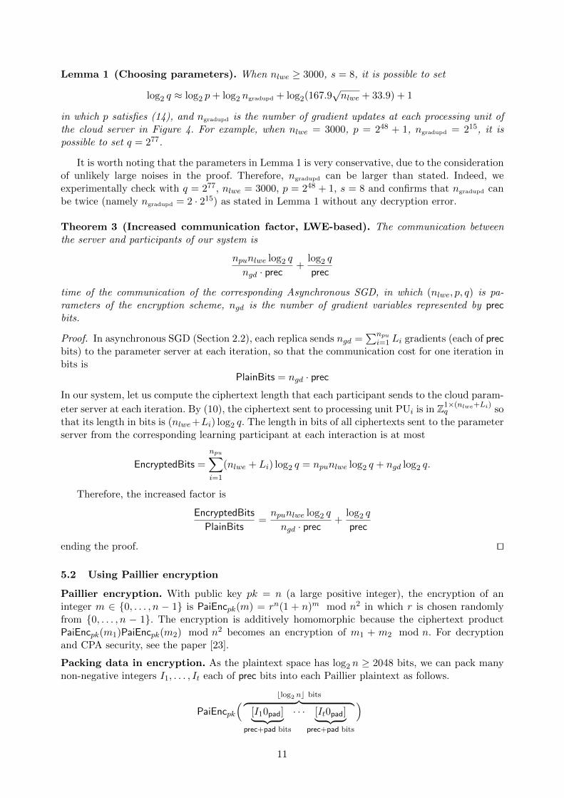
Lemma 1 (Choosing parameters). When nlwe ≥ 3000, s = 8, it is possible to set

log2 q ≈ log2 p+ log2 ngradupd + log2(167.9√nlwe + 33.9) + 1

in which p satisfies (14), and ngradupd is the number of gradient updates at each processing unit ofthe cloud server in Figure 4. For example, when nlwe = 3000, p = 248 + 1, ngradupd = 215, it ispossible to set q = 277.

It is worth noting that the parameters in Lemma 1 is very conservative, due to the considerationof unlikely large noises in the proof. Therefore, ngradupd can be larger than stated. Indeed, weexperimentally check with q = 277, nlwe = 3000, p = 248 + 1, s = 8 and confirms that ngradupd canbe twice (namely ngradupd = 2 · 215) as stated in Lemma 1 without any decryption error.

Theorem 3 (Increased communication factor, LWE-based). The communication betweenthe server and participants of our system is

npunlwe log2 q

ngd · prec+

log2 q

prec

time of the communication of the corresponding Asynchronous SGD, in which (nlwe, p, q) is pa-rameters of the encryption scheme, ngd is the number of gradient variables represented by precbits.

Proof. In asynchronous SGD (Section 2.2), each replica sends ngd =∑npu

i=1 Li gradients (each of precbits) to the parameter server at each iteration, so that the communication cost for one iteration inbits is

PlainBits = ngd · precIn our system, let us compute the ciphertext length that each participant sends to the cloud param-

eter server at each iteration. By (10), the ciphertext sent to processing unit PUi is in Z1×(nlwe+Li)q so

that its length in bits is (nlwe+Li) log2 q. The length in bits of all ciphertexts sent to the parameterserver from the corresponding learning participant at each interaction is at most

EncryptedBits =

npu∑

i=1

(nlwe + Li) log2 q = npunlwe log2 q + ngd log2 q.

Therefore, the increased factor is

EncryptedBits

PlainBits=npunlwe log2 q

ngd · prec+

log2 q

prec

ending the proof. ut

5.2 Using Paillier encryption

Paillier encryption. With public key pk = n (a large positive integer), the encryption of aninteger m ∈ {0, . . . , n − 1} is PaiEncpk(m) = rn(1 + n)m mod n2 in which r is chosen randomlyfrom {0, . . . , n − 1}. The encryption is additively homomorphic because the ciphertext productPaiEncpk(m1)PaiEncpk(m2) mod n2 becomes an encryption of m1 + m2 mod n. For decryptionand CPA security, see the paper [23].

Packing data in encryption. As the plaintext space has log2 n ≥ 2048 bits, we can pack manynon-negative integers I1, . . . , It each of prec bits into each Paillier plaintext as follows.

PaiEncpk

( blog2 nc bits︷ ︸︸ ︷[I10pad]︸ ︷︷ ︸

prec+pad bits

· · · [It0pad]︸ ︷︷ ︸prec+pad bits

)

11

in which 0pad is the zero padding of pad bits, which helps preventing overflows in ciphertext ad-ditions. Typically, pad ≈ log2 ngradupd as we need ngradupd additions of ciphertexts. Moreover, asthe number of plaintext bits must be less than log2 n, it is necessary that t(prec + pad) ≤ log2 n.Therefore,

t =

⌊ blog2 ncprec + pad

⌋

which is the upper-bound of packing prec-bit integers into one Paillier plaintext. To handle bothnegative and positive integers, we can use the bijection z ∈ [0, 2prec − 1] 7→ z − bz/2prece · 2prec.

As a real number 0 ≤ r < 1 can be represented as an integer of form br · 2precc, the abovepacking method can be used to encrypt around blog2 nc/(prec + pad) real numbers in the range[0, 1) with precision prec, tolerating around 2pad ciphertext additions.

To realise the encryption E(·) in Figure 4, it suffices to describe an encryption of a real vector

r = (r(1), . . . , r(Li)) ∈ RLi because both W(i)global and α · G(i) ∈ RLi in which

∑npu

i=1 Li = ngd. Theencryption E(r) consists of approximately dLi/te Paillier ciphertexts:

PaiEncpk

(blog2 nc bits︷ ︸︸ ︷

br(1) · 2precc0pad︸ ︷︷ ︸prec+pad bits

· · · br(t) · 2precc0pad︸ ︷︷ ︸prec+pad bits

), . . . ,PaiEncpk

(blog2 nc bits︷ ︸︸ ︷

br(Li−t+1) · 2precc0pad︸ ︷︷ ︸prec+pad bits

· · · br(Li) · 2precc0pad︸ ︷︷ ︸prec+pad bits

).

Theorem 4 (Increased communication factor, Paillier-based). The communication betweenthe server and participants of our system is

2

(1 +

pad

prec

)

times of the communication of the corresponding Asynchronous SGD, in which pad is the numberof 0 paddings to tolerate 2pad additions (equal to the number of gradient updates on the server),and prec is the bit precision of numbers.

Proof. In our system in Figure 4, each participant needs to encrypt and send at most∑npu

i=1 Li = ngdgradients to the server, in which Li is the length of G(i). Therefore, with the above packing methodfor Paillier encryption, the number of Paillier ciphertexts sent from each participant is around

npu∑

i=1

Lit≈ ngd

t≈ ngd(prec + pad)

blog2 nc.

Since each Paillier ciphertext is of 2blog2 nc bits, the number of bits for each communication isaround

EncryptedBits ≈ 2blog2 nc ·ngdt≈ 2ngd(prec + pad).

On the other hand, note that each replica in Asynchronous SGD needs to send ngd gradients eachof prec bits to the server, the communication cost in bits is PlainBits = ngd · prec. Therefore, theincreased factor is

EncryptedBits

PlainBits=

2ngd(prec + pad)

ngd · prec= 2

(1 +

pad

prec

)

as claimed. ut

6 Concrete evaluations with LWE-based encryption

We take nlwe = 3000, s = 8, p = 248 + 1, ngradupd = 215, and q = 277 following Lemma 1. Theseparameters for (nlwe, s, q) conservatively ensure that the LWE assumption has at least 128-bitsecurity according to recent attacks [6, 13, 19, 20]. We will take npu ∈ {1, 10}, depending on thenumber of gradients.

12

6.1 Increased factors in communication

Let us consider multiple number of gradient parameters ngd:

• ngd = 109386: this number of gradient parameters is used with the dataset MNIST [5]. Specifi-cally, consider an MLP with form 784 (input) – 128 (hidden) – 64 (hidden) – 10 (output). Thenumber of gradients for this network is (784+1)128+(128+1)64+(64+1)10 = 109386. We willconsider cases where real numbers are represented by 32 bits, so that prec = 32. Theorem 3 tellsus that the increased communication factor between our system and the related AsynchronousSGD is

npunlwe log2 q

ngd · prec+

log2 q

prec=

1 · 3000 · 77

109386 · 32+

77

32≈ 2.47.

• ngd = 402250: this is used in [26] with the dataset SVHN [22]. The increased communicationfactor becomes

npunlwe log2 q

ngd · prec+

log2 q

prec=

1 · 3000 · 77

402250 · 32+

77

32≈ 2.42.

• ngd = 42 ·106: this number of gradient parameters is used in [14] for speech data. As the numberof gradients is large, consider npu = 10. The increased communication factor becomes

npunlwe log2 q

ngd · prec+

log2 q

prec=

10 · 3000 · 77

42 · 106 · 32+

77

32≈ 2.4.

Our system with Paillier encryption. We take log2 n = 3072, pad = 15, so that the increasedcommunication factor becomes, via Theorem 4,

EncryptedBits

PlainBits= 2

(1 +

pad

prec

)= 2

(1 +

15

32

)≈ 2.93

which is independent of ngd.

6.2 Estimating the computational costs

To estimate the running time of our system, we use the following formulas

T(i)ours, one run = T

(i)original, one run + T(i)

enc + T(i)dec + T

(i)upload + T

(i)download + Tadd, (15)

Tour system =

N∑

i=1

n(i)upload/download ×T(i)

ours, one run (16)

where, in (15), T(i)ours, one run is the running time of the participant i when doing the following:

waiting for the addition of ciphertexts at the server (Tadd); download the added ciphertext from

the server (T(i)download); decrypted the downloaded ciphertext (T

(i)dec); training with the downloaded

weight (T(i)original, one run); encrypting the resulting gradients (T

(i)enc) and sending back that ciphertext

to the server (T(i)dec). The total running time of our system Tour system will be the sum of all N

participants’ running times, multiplied by the number nrepeat of repetitions, as expressed in (16).

Environment. Our codes for homomorphic encryption are in C++, and the benchmarks are overan Xeon CPU E5-2660 v3@ 2.60GHz server. To estimate the communication speed between eachlearning participants and the server, we assume a 1 Gbps network. To measure the running timeof MLP, we use the Tensorflow 1.1.0 library [4] over Cuda-8.0 and GPU Tesla K40m.

13

Table 3. LWE-based encryption scheme (nlwe = 3000, s = 8, p = 248 + 1, and q = 277) running times with variousnumbers of gradients.

Number of gradients ngd

20000 27882 50000 52650 100000 200000 300000 402250Processing time using 1 thread of computation

Enc. via (10) msec 164.4 213.1 364.6 454.8 732.9 1395.1 2031.6 2797.4

Dec. of (10) msec 143.6 194.5 354.6 412.6 666.1 1355.0 1996.5 2738.0

Add of ciphertexts via (11) usec 51 72.3 137.7 91.2 211.5 441.7 481.0 698.4

Processing time using 20 threads of computation

Enc. via (10) msec 30.2 50.8 93.2 70.3 188.9 415.8 587.8 875.4Dec. of (10) msec 31.9 44.7 85.8 78.5 196.0 460.5 644.9 820.9

Add of ciphertexts via (11) usec 9.5 11.1 15.8 14.0 19.5 38.7 41.1 56.4

Fig. 5. Computational costs of the LWE-based encryption and decryption when nlwe = 3000, s = 8, q = 277.

Time of encryption, decryption and addition. Table 3 gives the time for encryption, decryp-tion and addition depending on the number of gradients ngd, using nlwe = 3000, s = 8, p = 248 + 1,and q = 277. Figure 5 depicts the time of encryption and decryption using 1 thread and 20 threadsof computation respectively.

Multilayer Perceptron (MLP). Consider an MLP with form 784 (input) – 128 (hidden) – 64(hidden) – 10 (output). The number of gradients for this network is (784+1)128+(128+1)64+(64+1)10 = 109386. For 32-bit precision, these gradients are around 109386×32/(8×106) ≈ 0.437 MB inplain. The ciphertext of these gradients is of 0.437×2.47 ≈ 1.0 MB as computed in Section 6.1 whichcan be sent in around 0.008 seconds (= 8 ms) via an 1 Gbps communication channel. The original

running time of this MLP with one data batch of size 50 (MNIST images) is T(i)original, one run ≈ 4.6

(ms). Therefore,

T(i)ours, one run = T

(i)original, one run + T(i)

enc + T(i)dec + T

(i)upload + T

(i)download + Tadd

≈ 4.6 + 188.9 + 196.0 + 8 + 8 + 9.5/103 (ms)

≈ 405.5 (ms)

Suppose that there are totally 2×104 times of upload and download from all training participants

to the server, namely∑N

i=1 n(i)upload/download = 2 × 104. For simplicity suppose T

(i)ours, one run is the

same for all 1 ≤ i ≤ N . In such case, the running time of our system can be estimated as

Tour system = T(i)ours, one run × 2× 104 = 405.5× 2× 104 (ms) ≈ 2.25 (hours).

14

As seen in Theorem 2, the accuracy of our system can be identical to that of asynchronousSGD. Therefore, it suffices to estimate the accuracy of asynchronous SGD over MNIST containingrandomly shuffled 6 × 104 images for training and 104 images for testing. As above, the batchsize is 50. The initial weights are randomly selected from a normal distribution of mean 0 andstandard deviation 0.1 (via the function random normal of Tensorflow). The activation function isthe relu function in Tensorflow. The Adam optimizer (AdamOptimizer) is used for training withinput learning rate 10−4, with no drop out. After 2 × 104 iterations elapsed by 2 minutes, ourTensorflow code achieves around 97% accuracy over the testing set.

7 Conclusion

We show that, sharing gradients even partially over a parameter cloud server as in [26] may leak in-formation on data. We then propose a new system that utilises additively homomorphic encryptionto protect the gradients against the curious server. In addition to privacy-preserving, our systemenjoys the property of not declining the accuracy of deep learning.

Acknowlegment

This work is partially supported by Japan Science and Technology Agency CREST #JPMJCR168A.

References

1. Machine Learning Coursera’s course. https://www.coursera.org/learn/machine-learning.2. MNIST results. http://yann.lecun.com/exdb/mnist/.3. Stanford Deep Learning Tutorial. http://deeplearning.stanford.edu.4. Tensorflow. https://www.tensorflow.org.5. The MNIST dataset. http://yann.lecun.com/exdb/mnist/.6. Y. Aono, X. Boyen, L. T. Phong, and L. Wang. Key-private proxy re-encryption under LWE. In G. Paul and

S. Vaudenay, editors, Progress in Cryptology - INDOCRYPT 2013. Proceedings, volume 8250 of Lecture Notes inComputer Science, pages 1–18. Springer, 2013.

7. Y. Aono, T. Hayashi, L. T. Phong, and L. Wang. Privacy-preserving logistic regression with distributed datasources via homomorphic encryption. IEICE Transactions, 99-D(8):2079–2089, 2016.

8. Y. Aono, T. Hayashi, L. T. Phong, and L. Wang. Scalable and secure logistic regression via homomorphicencryption. In Proceedings of the Sixth ACM on Conference on Data and Application Security and Privacy,CODASPY, pages 142–144, 2016.

9. Y. Aono, T. Hayashi, L. T. Phong, and L. Wang. Efficient key-rotatable and security-updatable homomor-phic encryption. In Proceedings of the Fifth ACM International Workshop on Security in Cloud Computing,SCC@AsiaCCS 2017, pages 35–42, 2017.

10. Y. Aono, T. Hayashi, L. T. Phong, and L. Wang. Input and output privacy-preserving linear regression. IEICETransactions, 100-D(10), 2017.

11. W. Banaszczyk. New bounds in some transference theorems in the geometry of numbers. Mathematische Annalen,296(1):625–635, 1993.

12. W. Banaszczyk. Inequalities for convex bodies and polar reciprocal lattices in Rn. Discrete & ComputationalGeometry, 13(1):217–231, 1995.

13. I. Chillotti, N. Gama, M. Georgieva, and M. Izabachene. Faster fully homomorphic encryption: Bootstrappingin less than 0.1 seconds. In Advances in Cryptology - ASIACRYPT 2016 - 22nd International Conference on theTheory and Application of Cryptology and Information Security, Proceedings, Part I, pages 3–33, 2016.

14. J. Dean, G. Corrado, R. Monga, K. Chen, M. Devin, Q. V. Le, M. Z. Mao, M. Ranzato, A. W. Senior, P. A.Tucker, K. Yang, and A. Y. Ng. Large scale distributed deep networks. In P. L. Bartlett, F. C. N. Pereira, C. J. C.Burges, L. Bottou, and K. Q. Weinberger, editors, 26th Annual Conference on Neural Information ProcessingSystems 2012., pages 1232–1240, 2012.

15. J. Duchi, E. Hazan, and Y. Singer. Adaptive subgradient methods for online learning and stochastic optimization.J. Mach. Learn. Res., 12:2121–2159, July 2011.

16. R. Gilad-Bachrach, N. Dowlin, K. Laine, K. E. Lauter, M. Naehrig, and J. Wernsing. Cryptonets: Applyingneural networks to encrypted data with high throughput and accuracy. In M. Balcan and K. Q. Weinberger,editors, Proceedings of the 33nd International Conference on Machine Learning, ICML 2016, New York City, NY,USA, June 19-24, 2016, volume 48 of JMLR Workshop and Conference Proceedings, pages 201–210. JMLR.org,2016.

15

17. O. Goldreich. The Foundations of Cryptography - Volume 2, Basic Applications. Cambridge University Press,2004.

18. B. Hitaj, G. Ateniese, and F. Perez-Cruz. Deep models under the GAN: information leakage from collaborativedeep learning. CoRR, abs/1702.07464, 2017.

19. R. Lindner and C. Peikert. Better key sizes (and attacks) for LWE-based encryption. In A. Kiayias, editor, Topicsin Cryptology - CT-RSA 2011, volume 6558 of Lecture Notes in Computer Science, pages 319–339. Springer, 2011.

20. M. Liu and P. Q. Nguyen. Solving BDD by enumeration: An update. In E. Dawson, editor, Topics in Cryptology- CT-RSA 2013. Proceedings, volume 7779 of Lecture Notes in Computer Science, pages 293–309. Springer, 2013.

21. P. Mohassel and Y. Zhang. Secureml: A system for scalable privacy-preserving machine learning. In 2017 IEEESymposium on Security and Privacy, pages 19–38, 2017.

22. Y. Netzer, T. Wang, A. Coates, A. Bissacco, B. Wu, and A. Y. Ng. Reading digits in natural images withunsupervised feature learning. In NIPS Workshop on Deep Learning and Unsupervised Feature Learning 2011,2011.

23. P. Paillier. Public-key cryptosystems based on composite degree residuosity classes. In J. Stern, editor, Advancesin Cryptology - EUROCRYPT ’99, Proceeding, volume 1592 of Lecture Notes in Computer Science, pages 223–238. Springer, 1999.

24. L. T. Phong, Y. Aono, T. Hayashi, L. Wang, and S. Moriai. Privacy-preserving deep learning: Revisited andenhanced. In Applications and Techniques in Information Security - 8th International Conference, ATIS 2017,Proceedings, pages 100–110, 2017.

25. B. Recht, C. Re, S. J. Wright, and F. Niu. Hogwild: A lock-free approach to parallelizing stochastic gradientdescent. In J. Shawe-Taylor, R. S. Zemel, P. L. Bartlett, F. C. N. Pereira, and K. Q. Weinberger, editors, NIPS2011, pages 693–701, 2011.

26. R. Shokri and V. Shmatikov. Privacy-preserving deep learning. In I. Ray, N. Li, and C. Kruegel, editors,Proceedings of the 22nd ACM SIGSAC Conference on Computer and Communications Security, 2015, pages1310–1321. ACM, 2015.

A CPA security of the LWE-based homomorphic encryption scheme

We first recall the definition of CPA security.

Definition 2. (CPA security) With respect to a PHE scheme as in Definition 1, consider thefollowing game between an adversary A and a challenger:

• Setup. The challenger creates pp and key pairs (pk, sk). Then pp and pk are given to A.• Challenge. A chooses two plaintexts m0,m1 of the same length, then submits them to the chal-

lenger, who in turn takes b ∈ {0, 1} randomly and computes C∗ = Enc(pk,mb). The challengeciphertext C∗ is returned to A, who then produces a bit b′.

A PHE scheme is secure against chosen plaintext attacks (CPA-secure) if the advantage

AdvcpaA (λ) =

∣∣∣∣Pr[b′ = b]− 1

2

∣∣∣∣

is negligible in λ.

Related to the decision LWE assumption LWE(nlwe, s, q), where nlwe, s, q is the parameter for

security, consider matrix A$← Zm×nlwe

q , vectors r$← Zm×1q , x

g← Znlwe×1(0,s) , e

g← Zm×1(0,s) . Then vectorAx+ e is computed over Zq. Define the following advantage of a poly-time probabilistic algorithmD:

AdvLWE(nlwe,s,q)D (λ) =

∣∣∣Pr[D(A,Ax+ e)→ 1]− Pr[D(A, r)→ 1]∣∣∣.

The LWE assumption asserts that AdvLWE(nlwe,s,q)D (λ) is negligible as a function of λ.

Claim. The additively homomorphic encryption scheme in Section 5.1 is CPA-secure under theLWE assumption. Specifically, for any poly-time adversary A, there is an algorithm D of essentiallythe same running time such that

AdvcpaA (λ) ≤ (l + 1) ·Adv

LWE(nlwe,s,q)D (λ).

16

Proof. The proof has been in [9] and is given here for completeness. First, we modify the original

game in Definition 2 by providing A with a random P$← Znlwe×l

q . Namely P = pR−AS ∈ Znlwe×lq

is turned to random. This is indistinguishable to A thanks to the LWE assumption with secretvectors as l columns of S. More precisely, we need the condition gcd(p, q) = 1 to reduce P =pR − AS ∈ Znlwe×l

q to the LWE form. Indeed, p−1P = R + (−p−1A)S ∈ Znlwe×lq . As A is random,

A′ = −p−1A ∈ Znlwe×nlweq is also random. Therefore, P ′ = p−1P ∈ Znlwe×l

q is random under theLWE assumption which in turn means P is random as claimed.

Second, the challenge ciphertext c∗ = e1[A|P ]+p[e2|e3]+[0|mb] is turned to random. This relieson the LWE assumption with secret vector e1, while also basing on the first modification so that[A|P ] is a random matrix. Here, the condition gcd(p, q) = 1 is also necessary as above. Thus b isperfectly hidden after this change. The factor l + 1 is due to l uses of LWE in changing P and 1use in changing c∗. ut

B Proof of Lemma 1

We will use following lemmas [11,12,19]. Below 〈·, ·〉 stands for inner product. Writing ||Zn(0,s)|| is ashort hand for taking a vector from the discrete Gaussian distribution of deviation s and computingits Euclidean norm.

Lemma 2. Let c ≥ 1 and C = c · exp(1−c2

2 ). Then for any real s > 0 and any integer n ≥ 1, wehave

Pr

[||Zn(0,s)|| ≥

c · s√n√2π

]≤ Cn.

Lemma 3. For any real s > 0 and T > 0, and any x ∈ Rn, we have

Pr[||〈x,Zn(0,s)〉|| ≥ Ts||x||

]< 2 exp(−πT 2).

Proof (Proof of Claim 1). Suppose cadd =∑nadd

i=1 c(i) =∑nadd

i=1 (c(i)1 , c

(i)2 ) is the additions of nadd

ciphertexts. In Claim 1, nadd = ngradupd. Its decryption is

madd =

nadd∑

i=1

[c(i)1 S + c

(i)2

]

=

nadd∑

i=1

[(e

(i)1 A+ pe

(i)2 )S + e

(i)1 P + pe

(i)3 +m(i)

]

=

nadd∑

i=1

[e(i)1 (AS + P ) + p(e

(i)2 S + e

(i)3 ) +m(i)

]

=

nadd∑

i=1

[p(e

(i)1 R+ e

(i)2 S + e

(i)3 ) +m(i)

]∈ Z1×l

q

Therefore, the accumulative noise after nadd ciphertext additions is

Noise = p

nadd∑

i=1

(e(i)1 R+ e

(i)2 S + e

(i)3 ) ∈ Z1×l

q

The term e(i)1 R+e

(i)2 S+e

(i)3 ∈ Z1×l

q has l components, each of which can be written as the innerproduct of two vectors of form

e = (e(i)1 , e

(i)2 , e

(i)3 )

x = (r, r′,0101×l)

where,

17

– vectors e(i)1

g← Z1×nlwe

(0,s) , e(i)2

g← Z1×nlwe

(0,s) , and e(i)3

g← Z1×l(0,s)

– vectors r, r′g← Z1×nlwe

(0,s) represent corresponding columns in matrices R,S; and 0101×l stands fora vector of length l with all 0’s except one 1.

We have

e ∈Z1×(2nlwe+l)(0,s)

||x|| ≤||(r, r′)||+ 1.

Applying Lemma 2 for the above vector (r, r′) of length 2nlwe, with overwhelming probability of

1− C2nlwe(≥ 1− 2−80 for our choices of parameters)

we have

||x|| ≤ c · s√2nlwe√2π

+ 1.

We now use Lemma 3 with vectors x and e. Let ρ be the error per message symbol in decryption,we set 2 exp(−πT 2) = ρ, so T =

√ln(2/ρ)/

√π. The bound on the inner product 〈x, e〉 becomes

Ts||x||, which is not greater than

U =s√

ln(2/ρ)√π

(c · s√2nlwe√

2π+ 1

)

so that each component in Noise ∈ Z1×lq will be less than

B = pnadd · U.

For correctness, it suffices to set B = q/2, namely q = 2B. This means

log2 q = log2 p+ log2 nadd + log2(U) + 1.

We take c = 1.1 so that C2nlwe < 2−80 when nlwe ≥ 3000. Also take ρ = 2−80, s = 8 so that

U = 167.9106√nlwe + 33.8197

and the proof follows. ut

18