Probabilistic Calculus to the Rescue

Suppose we know the likelihood of each of the (propositional)

worlds (aka Joint Probability distribution )

Then we can use standard rules of probability to compute the likelihood of all queries (as I will remind you)

So, Joint Probability Distribution is all that you ever need!

In the case of Pearl example, we just need the joint probability distribution over B,E,A,J,M (32 numbers)--In general 2n separate numbers

(which should add up to 1)

If Joint Distribution is sufficient for reasoning, what is domain knowledge supposed to help us with?

--Answer: Indirectly by helping us specify the joint probability distribution with fewer than 2n numbers

---The local relations between propositions can be seen as “constraining” the form the joint probability distribution can take!

Burglary => Alarm Earth-Quake => Alarm Alarm => John-callsAlarm => Mary-calls

Only 10 (instead of 32) numbers to specify!

Easy Special Cases

• If in addition, each proposition is equally likely to be true or false, – Then the joint probability

distribution can be specified without giving any numbers!

• All worlds are equally probable! If there are n props, each world will be 1/2n probable

– Probability of any propositional conjunction with m (< n) propositions will be 1/2m

• If there are no relations between the propositions (i.e., they can take values independently of each other)– Then the joint probability

distribution can be specified in terms of probabilities of each proposition being true

– Just n numbers instead of 2n

Will we always need 2n numbers?

• If every pair of variables is independent of each other, then– P(x1,x2…xn)= P(xn)* P(xn-1)*…P(x1)– Need just n numbers!– But if our world is that simple, it would also be very uninteresting & uncontrollable

(nothing is correlated with anything else!)

• We need 2n numbers if every subset of our n-variables are correlated together– P(x1,x2…xn)= P(xn|x1…xn-1)* P(xn-1|x1…xn-2)*…P(x1)– But that is too pessimistic an assumption on the world

• If our world is so interconnected we would’ve been dead long back…

A more realistic middle ground is that interactions between variables are contained to regions. --e.g. the “school variables” and the “home variables” interact only loosely (are independent for most practical purposes) -- Will wind up needing O(2k) numbers (k << n)

Directly usingJoint Distribution

Directly usingBayes rule

Using Bayes ruleWith bayes nets

Takes O(2n) for most natural queries of type P(D|Evidence)NEEDS O(2n) probabilities as input Probabilities are of type P(wk)—where wk is a world

Can take much less than O(2n) time for most natural queries of type P(D|Evidence)STILL NEEDS O(2n) probabilities as input Probabilities are of type P(X1..Xn|Y)

Can take much less than O(2n) time for most natural queries of type P(D|Evidence)Can get by with anywhere between O(n) and O(2n) probabilities depending on the conditional independences that hold. Probabilities are of type P(X1..Xn|Y)

Prob. Prop logic: The Game plan• We will review elementary “discrete variable” probability• We will recall that joint probability distribution is all we need to answer

any probabilistic query over a set of discrete variables.• We will recognize that the hardest part here is not the cost of inference

(which is really only O(2n) –no worse than the (deterministic) prop logic– Actually it is Co-#P-complete (instead of Co-NP-Complete) (and the former is

believed to be harder than the latter)• The real problem is assessing probabilities.

– You could need as many as 2n numbers (if all variables are dependent on all other variables); or just n numbers if each variable is independent of all other variables. Generally, you are likely to need somewhere between these two extremes.

– The challenge is to • Recognize the “conditional independences” between the variables, and exploit them

to get by with as few input probabilities as possible and • Use the assessed probabilities to compute the probabilities of the user queries efficiently.

Propositional Probabilistic Logic

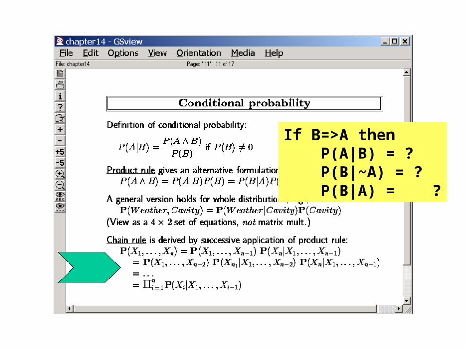
If B=>A then P(A|B) = ? P(B|~A) = ? P(B|A) = ?

CONDITIONAL PROBABLITIES

Non-monotonicity w.r.t. evidence– P(A|B) can be either higher, lower or equal to P(A)

Most useful probabilistic reasoning involves computing posterior

distributions

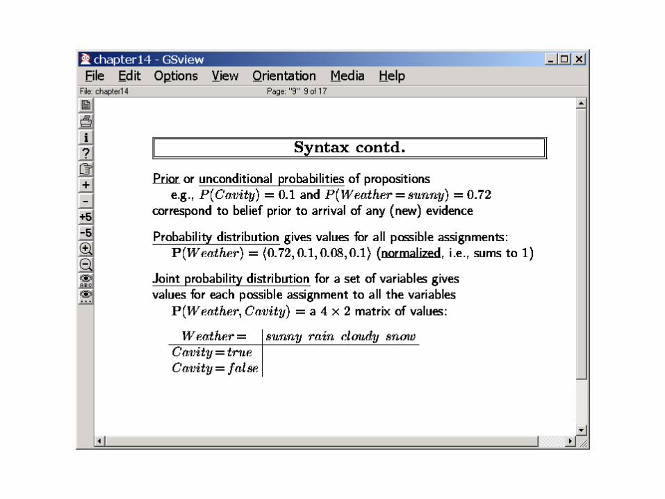
Probabilit

y

Variable values

P(A)

P(A|B=T)P(A|B=T;C=False)

Important: Computing posterior distribution is inference; not learning

If you know th

e full j

oint,

You can answ

er ANY query

& Marginalization

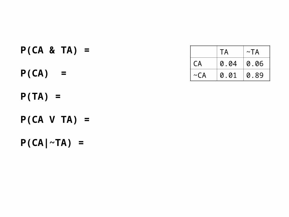
TA ~TA

CA 0.04 0.06

~CA 0.01 0.89

P(CA & TA) =

P(CA) =

P(TA) =

P(CA V TA) =

P(CA|~TA) =

TA ~TA

CA 0.04 0.06

~CA 0.01 0.89

P(CA & TA) = 0.04

P(CA) = 0.04+0.06 = 0.1 (marginalizing over TA)

P(TA) = 0.04+0.01= 0.05

P(CA V TA) = P(CA) + P(TA) – P(CA&TA) = 0.1+0.05-0.04 = 0.11

P(CA|~TA) = P(CA&~TA)/P(~TA) = 0.06/(0.06+.89) = .06/.95=.0631

Think of this as analogous to entailment by truth-table enumeration!

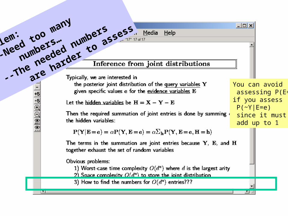
Problem:

--Need too many

numbers…

--The needed numbers

are harder to assess

You can avoid assessing P(E=e)if you assess P(~Y|E=e) since it must add up to 1

Happy Spring Break!

3/5

Homework 2 due todayMid-term on Tuesday after Springbreak

Will cover everything upto (but not including) probabilistic reasoning

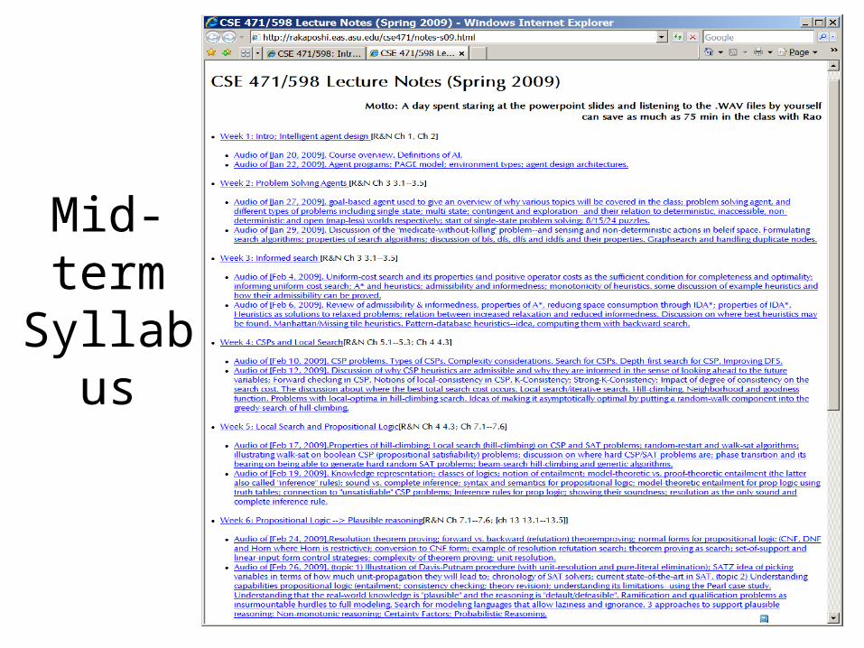
Mid-term Syllabus

Reviewing Last Class

• What is the difficult part of reasoning with uncertainty?– Complexity of reasoning?– Assessing Probabilities?

• If Joint distribution is enough for answering all queries, what exactly is the role of domain knowledge?

• What, if any, is the difference between probability and statistics? – Statistics Model-finding (learning)– Probability Model-using (inference)– Given your midterm marks, I am interested in finding the model of the generative

process that generated those marks. I will go ahead and use the assumption that each of your performance is independent of others in the class (clearly bogus since I taught you all), and another huge bias that the individual distributions are all Gaussian. Then I just need to find the mean and standard deviation for the data to give the full distribution.

– Given the distribution, now I can compute random queries the probability of more than 10 people getting more than 50 marks on the test!

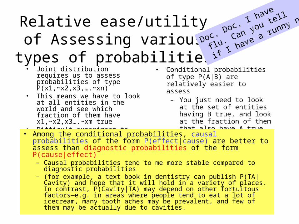
Relative ease/utility of Assessing various types of probabilities• Joint distribution requires us to assess

probabilities of type P(x1,~x2,x3,….~xn)

• This means we have to look at all entities in the world and see which fraction of them have x1,~x2,x3….~xm true

• Difficult experiment to setup..

• Conditional probabilities of type P(A|B) are relatively easier to assess

– You just need to look at the set of entities having B true, and look at the fraction of them that also have A true

– Eventually, they too can get baroque P(x1,~x2,…xm|y1..yn)

• Among the conditional probabilities, causal probabilities of the form P(effect|cause) are better to assess than diagnostic probabilities of the form P(cause|effect)– Causal probabilities tend to me more stable compared to diagnostic

probabilities– (for example, a text book in dentistry can publish P(TA|Cavity) and hope

that it will hold in a variety of places. In contrast, P(Cavity|TA) may depend on other fortuitous factors—e.g. in areas where people tend to eat a lot of icecream, many tooth aches may be prevalent, and few of them may be actually due to cavities.

Doc, Doc, I have

flu. Can you tell

if I have a runny nose?

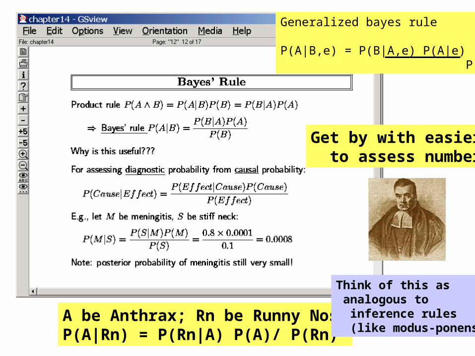
A be Anthrax; Rn be Runny NoseP(A|Rn) = P(Rn|A) P(A)/ P(Rn)

Get by with easier to assess numbers

Generalized bayes rule

P(A|B,e) = P(B|A,e) P(A|e) P(B|e)

Think of this as analogous to inference rules (like modus-ponens)

Can we avoid assessing P(S)?

P(M|S) = P(S|M) P(M)/P(S)

P(~M|S) = P(S|~M) P(~M)/P(S)

---------------------------------------------------------------- 1 = 1/P(S) [ P(S|M) P(M) + P(S|~M) P(~M) ] So, if we assess P(S|~M), then we don’t need to assess P(S)

“Normalization”

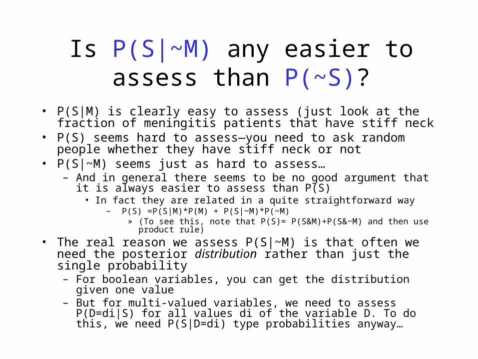
Is P(S|~M) any easier to assess than P(~S)?

• P(S|M) is clearly easy to assess (just look at the fraction of meningitis patients that have stiff neck

• P(S) seems hard to assess—you need to ask random people whether they have stiff neck or not

• P(S|~M) seems just as hard to assess…– And in general there seems to be no good argument that it is always easier

to assess than P(S)• In fact they are related in a quite straightforward way

– P(S) =P(S|M)*P(M) + P(S|~M)*P(~M)» (To see this, note that P(S)= P(S&M)+P(S&~M) and then use product rule)

• The real reason we assess P(S|~M) is that often we need the posterior distribution rather than just the single probability– For boolean variables, you can get the distribution given one value– But for multi-valued variables, we need to assess P(D=di|S) for all values

di of the variable D. To do this, we need P(S|D=di) type probabilities anyway…

What happens if there are multiple symptoms…?

Patient walked in and complained of toothache

You assess P(Cavity|Toothache)

Now you try to probe the patients mouth with that steel thingie, and it catches…

How do we update our belief in Cavity?

P(Cavity|TA, Catch) = P(TA,Catch| Cavity) * P(Cavity)

P(TA,Catch)

= P(TA,Catch|Cavity) * P(Cavity)Need to know this!If n evidence variables,We will need 2n probabilities!

Conditional independenceTo the rescue Suppose P(TA,Catch|cavity) = P(TA|Cavity)*P(Catch|Cavity)

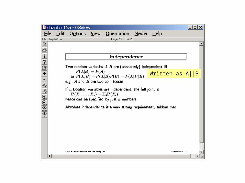
Written as A||B

Conditional Independence Assertions

• We write X || Y | Z to say that the set of variables X is conditionally independent of the set of variables Y given evidence on the set of variables Z (where X,Y,Z are subsets of the set of all random variables in the domain model)

• We saw that Bayes Rule computations can exploit conditional independence assertions. Specifically, – X || Y| Z implies

• P(X & Y|Z) = P(X|Z) * P(Y|Z)• P(X|Y, Z) = P(X|Z)• P(Y|X,Z) = P(Y|Z)

– If A||B|C then P(A,B,C)=P(A|B,C)P(B,C) =P(A|B,C)P(B|C)P(C) =P(A|C)P(B|C)P(C) (Can get by with 1+2+2=5 numbers instead of 8)

Why not write down all conditional independence assertions that hold in a domain?

Cond. Indep. Assertions (Contd)

• Idea: Why not write down all conditional independence assertions (CIA) (X || Y | Z) that hold in a domain?

• Problem: There can be exponentially many conditional independence assertions that hold in a domain (recall that X, Y and Z are all subsets of the domain variables).

• Many of them might well be redundant– If X||Y|Z, then X||Y|Z+U for all U

• Brilliant Idea: May be we should implicitly specify the CIA by writing down the “local dependencies” between variables using a graphical model

– A Bayes Network is a way of doing just this. • The Bayes Net is a Directed Acyclic Graph whose nodes are random variables, and the

immediate dependencies between variables are represented by directed arcs– The topology of a bayes network shows the inter-variable dependencies. Given the

topology, there is a way of checking if any Cond. Indep. Assertion. holds in the network (the Bayes Ball algorithm and the D-Sep idea)

CIA implicit in Bayes Nets

• So, what conditional independence assumptions are implicit in Bayes nets?– Local Markov Assumption:

• A node N is independent of its non-descendants (including ancestors) given its immediate parents. (So if P are the immediate paretnts of N, and A is a subset of of Ancestors and other non-descendants, then {N} || A| P )

• (Equivalently) A node N is independent of all other nodes given its markov blanket (parents, children, children’s parents)

– Given this assumption, many other conditional independencies follow. For a full answer, we need to appeal to D-Sep condition and/or Bayes Ball reachability

Topological Semantics

Indep

enden

ce fr

om

Non-d

esce

dants

holds

Given ju

st th

e par

ents

Indep

enden

ce fr

om

Every

nod

e hold

s

Given m

arkov

blan

ket

These two conditions are equivalent Many other conditional indepdendence assertions follow from these

Markov Blanket Parents;Children;Children’s other parents