Probabilistic Constraint Handling in the Framework of JointEvolutionary-Classical Optimization with Engineering Applications

Rituparna Datta, Michael S. Bittermann, Kalyanmoy Deb (IEEE Fellow) and Ozer CiftciogluKanGAL Report Number 2012006

Abstract—Optimization for single main objective with multiconstraints is considered using a probabilistic approach coupledto evolutionary search. In this approach the problem is convertedinto a bi-objective problem, treating the constraint ensemble asa second objective subjected to multi-objective optimization forthe formation of a Pareto front, and this is followed by a localsearch for the optimization of the main objective function. In thisprocess a novel probabilistic modeling is applied to the constraintensemble, so that the stiff constraints are effectively taken careof, while the model parameter is adaptively determined duringthe evolutionary search. In this way the convergence to thesolution is significantly accelerated and an accurate solutionis established. The improvements are demonstrated by meansof example problems including comparisons with the standardbenchmark problems, the solutions of which are reported in theliterature.

I. Introduction

MANY real life problems involve decision makings andchoices based on some compromises. Among the pos-

sible compromises to select the ones which are as good aspossible is a natural way to proceed. In general this process iscomplex and it can be defined as optimization. The complexityarises due to a single or many conflicting objectives. Mostreal-life problems in science, engineering and optimizationconsist of one or many linear, non-linear, non-convex, anddiscontinuous constraints, which come into picture mainlydue to some physical limitations or functional requirementsto satisfy. Constraints can be subdivided into inequality typeor equality type, but the challenge is to satisfy all constraintsto make the solution be feasible. To solve the optimizationproblems traditionally a number of methods are developedin the realm of mathematics with their associated meritsand limitations [1], [2], [3]. With modern advancements inscience and engineering, from last two decades the solutionof optimization problems are sought by means of evolutionarysearch algorithms which are proved to be very effective [4],[5], [6]. Even though evolutionary algorithms mainly weredeveloped to solve unconstrained problems, researchers suc-

Rituparna Datta is doctoral student at Department of Mechanical Engi-neering, Indian Institute of Technology Kanpur, PIN 208016, India (email:rdatta@iitk.ac.in)

Michael S. Bittermann is post doctoral research scholar at at Chairof Design Informatics (TO&I), Department of Building Technology, DelftUniversity of Technology, 2628 BL Delft (email: m.s.bittermann@tudelft.nl)

Kalyanmoy Deb (Fellow, IEEE) is professor, Department of MechanicalEngineering, Indian Institute of Technology Kanpur, PIN 208016, India(email: deb@iitk.ac.in)

Ozer Ciftcioglu (Sr. Member, IEEE) is professor at Chair of DesignInformatics (TO&I), Department of Building Technology, Delft Universityof Technology, 2628 BL Delft (email: O.Ciftcioglu@tudelft.nl)

cessfully introduced many constraint handling mechanisms tosolve constrained optimization problems [7], [8], [9].

A constrained optimization problem is generally formulatedas the following non-linear programming (NLP) problem:

Minimize / Maximize f (x),Subject to g j(x) ≥ 0, j = 1, .., J,

hk(x) = 0, k = 1, ..,K,xl

i ≤ xi ≤ xui , i = 1, .., n.

(1)

In the NLP problem, n is the number of variables, J thenumber of inequality constraints, and K the number of equalityconstraints. The function f (x) is the objective (cost) function,the j-th inequality constraint is g j(x) and hk(x) is the k-thequality constraint. The range of i-th variable varies in between[xl

i, xui ]. In this work exclusively inequality constraints are

treated. To handle an equality constraint the same methodologycan be used under the condition that the equality constraintis approximated by a corresponding inequality constraint asfollows: gJ+k(x) = |εk − hk(x)| ≥ 0, where εk represents a smalltolerance for violation of the original equality constraint.

Identifying a solution x that is both feasible and optimizesthe objective at hand is particularly challenging when con-straints and objective have a non-linear, non-convex, discrete,or non-differentiable nature. Solving such an engineeringproblem is formidably challenging when classical optimizationalgorithms and theorems are used, as these are developedmainly for well-behaved problems [4], [10], [11]. The reasonfor this is that the non-linearity in the objective and constraintfunctions gives rise to many local optima. Therefore a classicalalgorithm, being based on improving a single solution inobjective space, is generally bound to be trapped in one of thelocal optima and not reach the global optimum. Evolutionarycomputation was found to be able to handle such problems dueto its stochastic, population-based nature, where it probes thespace of possible solutions at several points simultaneously,without making use of derivative information. The basicprinciple of an evolutionary algorithm (EA) is to improveindividuals of a randomly generated initial population based oncombining potentially successful ones. The combination yieldsnew solutions in the vicinity of the original solutions, whilethe new solutions may outperform the previous ones. Thisprinciple turned out to be generically capable for optimiza-tion problems with non-linear or discrete objective functions,so that evolutionary algorithms have been used for variousengineering applications, e.g. [7], [12], [13].

Deb [8] developed an evolutionary algorithm for constrained

optimization problems. In this approach, during the tourna-ment selection process, an infeasible solution is always treatedas inferior compared to a feasible one, or as inferior comparedto a solution that violates the constraints to a lesser extent. Inthis algorithm, among two infeasible solutions, exclusively thedifference in the amount of violating a constraint determinesthe suitability of a solution, so that the information on objec-tive function value is not taken into account. This may lead tofeasible solutions, which however do not yield satisfactory ob-jective function values. With increasing difficulty of a problem,i.e. as the degree of non-linearity of objectives and constraintsincreases, it becomes aparent that evolutionary computationhas limited robustness and effectiveness, which is partially dueto ineffective constraint handling in the algorithms. Namely,when the feasible region is sufficiently small compared to thespace of possible solutions, then an initial population of anevolutionary algorithm generally does not contain any feasiblesolution. This lack of information in the population poses achallenge to the algorithm as it aims to reach to the feasibleregion in the search domain. The problem is to assess thepotential of a solution in the population, for reaching thefeasible region while satisfying the objective at the same time.

An approach to make use of constraint information andobjective information at the same time without merging themby means of a linear combination, is to consider the con-strained single objective problem as a bi-objective optimizationproblem. This means, next to the original single objectivef (x) a measure of overall constraint violation is used asan additional objective to be minimized [14]. This way thesearch process tolerates infeasible solutions as long as they arePareto-optimal regarding function value as well as constraintviolation. This approach is also referred to as ’multiobjec-tivization’ [15]. Through multiobjectivization the informationin the population is exploited more effectively compared tothe previously mentioned approaches. Recently an extensionof the bi-objective approach was proposed [16] using thereference point approach to focus the search in the vicinity ofthe constrained minimum solution. Wang et al. [17] proposedan adaptive trade off model (ATM) using bi-objective approachwith three phase methodology for handling constraints inevolutionary optimization.

Studies on many different evolutionary algorithms for con-strained optimization showed that finding the constrainedoptimum by an evolutionary algorithm alone is problematic formultiple, non-linear constraints, so that it became appealingto use evolutionary algorithms jointly with a classical localsearch procedure [18]. Recently, a bi-objective evolutionaryoptimization strategy has been proposed [9] to estimate thepenalty parameter R for a problem from the obtained two-objective non-dominated front. Based on the informationobtained through the bi-objective evolutionary algorithm, anappropriate penalized function is constructed and solved usinga classical local search method. Another joint evolutionary-classical method used gradient information of the constraintsto repair the solutions which are not feasible [19]. Yet an-other joint approach used the combination of Nelder-Mead

simplex search with evolutionary algorithm [20]. More hybridconstraint handling studies can be found in [21], [22].

Presumably the most popular constraint handling approachis known as the penalty function approach, which was orig-inally developed for the classical optimization methodolo-gies. A penalty function penalizes a solution by worseningthe fitness of a solution, when it violates constraints. Thispenalization is accomplished by adding a value to a solu-tion’s objective function value in proportion to the amountof constraint violation. The proportionality factor is known asthe penalty parameter, which balances the relative importancebetween constraint violation and objective function value.That is, in the penalty method a constrained optimizationproblem is converted into an unconstrained problem. Thisapproach is very popular presumably due to the simplicity ofthe concept and ease of implementation. However, it is clearlynoted that fixing a penalty parameter implies that the relativeimportance among constraint violation and satisfaction of theobjective function should be known, which is a problematicissue in general due to non-linearity inherent to objective andconstraint functions. To overcome this issue to some extend,Coello [23] proposed a self-adaptive penalty approach by usinga co-evolutionary model to adapt the penalty factors.

In this paper an approach is proposed where constraintviolation is treated in probabilistic terms. This way, the popu-lation based nature of the evolutionary algorithm is exploited,in order to estimate the relative significance of violating aconstraint in perspective with the other constraints.

The organization of the paper is as follows. In the nextsection a probabilistic method developed in this work isdescribed. Thereafter its effectiveness is verified by means ofapplications of the associated algorithm for solving a numberof mathematical test problems, an engineering design problem,and a robotics problem. This is followed by conclusions.

II. Evolutionary Optimization and Probabilistic ConstraintHandling

The bi-objective joint evolutionary-classical method usedin this work is a combination of a multiobjectivized EA andthe penalty function approach for inequality constraints. Themethod has been described elsewhere [9]. Additionally, inthis work a probabilistic model is developed associated withthe Pareto front formed by the objective function and theconstraint violation. Based on this model the penalty parameterover all constraint violation is computed in a natural way,so that commensurate weighting of the constraint violation ismaintained throughout the optimizations process. The antici-pated outcome is the effective solution for the problem at handwith major improvements compared to the several approachesmentioned above. For convenience of readers the essentialissues of the bi-objective joint approach are pointed out inthe following section before addressing the novel probabilisticconstraint handling technique.

A. Bi-objective approach

The working principle of evolutionary-classical algorithmproposed in this work is based on bi-objective method ofhandling constrained single objective optimization problem,where a penalty function approach is used. In both evolu-tionary and classical search, a novel probabilistic constrainthandling approach is employed that will be described in thenext subsection. The algorithm is described as follows, clar-ifying the role of its evolutionary, probabilistic and classicalcomponents.

First, the generation counter is set at t = 0.Step 1:The evolutionary component is an elitist, non-

dominated-sorting based multi-objective genetic al-gorithm (NSGA-II [6]). It is applied to the bi-objective optimization problem [9]. This meansthe Pareto-optimal solutions in the objective spaceformed by function value and constraint violation areto be identified. That is, the bi-objective problem isdefined as follows:

Minimize f (x),Minimize V(x),subject to x(L)

i ≤ xi ≤ x(U)i , i = 1, .., n.

(2)

where n denotes the number of variables, x(L)i and

x(U)i are the lower and upper variable bounds of the

i-th component of x respectively, and V(x) denotesthe overall constraint violation whose computationwe will describe in the next section.

Step 2:If t > 0 and ((t mod τ) = 0), the penalty parameterR is obtained from the current non-dominated frontas follows [9]. A cubic curve is fitted for the non-dominated points ( f = a+b×V +c×V2 +d×V3). Thisway the penalty parameter is estimated by finding theslope at V=0, that is R = −b. Since this is a lowerbound on R, after some trial-and-error experimentson standard test problems, twice this value is chosenas R, i.e. R = −2b [9].

Step 3:Thereafter, using R computed in Step 2, the followinglocal search problem is solved starting with the mostfeasible solution, i.e. the solution having minimumV(x), as given by

Minimize P(x) = f (x) + R × V(x),x(L)

i ≤ xi ≤ x(U)i .

(3)

The solution from the local search is denoted by x.Step 4:The algorithm is terminated in case x is feasible, and

the difference between two consecutive local searchsolutions is smaller than a small number δ f . In theapplications of this paper, δ f = 10−4 is used. Thenx is identified as the optimized solution. Else, t isincremented by one, and we continue with Step 1

It is noted that due to Step 2, the penalty parameter R is nota user-tunable parameter as it is determined from the obtainednon-dominated front. For the local search procedure in Step

3 Matlab’s fmincon() procedure with reasonable parametersettings is used to solve the penalized function.

B. Probabilistic constraint handling

Typically the penalty function approach is used to solve thefollowing unconstrained problem [9].

Minimize P(x,R) = f (x) +∑J

i=1 R j〈g j(x)〉. (4)

where f (x) is the objective function to be minimized; 〈α〉is the bracket operator and is equal to −α, if α〈0 and zerootherwise; g j(x) represents a general violation of the j-thconstraint. R j is the penalty parameter for j-th constraint.Since 〈g j(x)〉 is continually tried to be vanishing during theminimization process, probability density value of 〈g j(x)〉 ishighest at zero and its values gradually diminish. With thisinformation we can confidently surmise a probabilistic modelfor this probability density (pdf) which is exponential pdfgiven by

fλ(y) = λ e−λy. (5)

where λ is the decay parameter. If we denote 〈g j(x)〉 byv j(x), namely

〈g j(x)〉 = v j(x). (6)

the pdf in (5) becomes

fλ j(v j) = λ e−λ jv j . (7)

The mean value of the exponential pdf function is equal toλ−1

j . During the evolutionary search 〈g j(x)〉 is a general formof violation which applies to any member s of the populationalthough this is not explicitly denoted. In explicit form, wecan write

fλ j(v j,s) = λ j e−λ jv j,s . (8)

We can characterize the exponential pdf function accordingto the constraint j simply by equating the mean value of theviolations to the mean of the exponential pdf, namely

λ j = 1v j. (9)

so that (3) becomes

fλ j(v j) = 1v j

e−v j/v j . (10)

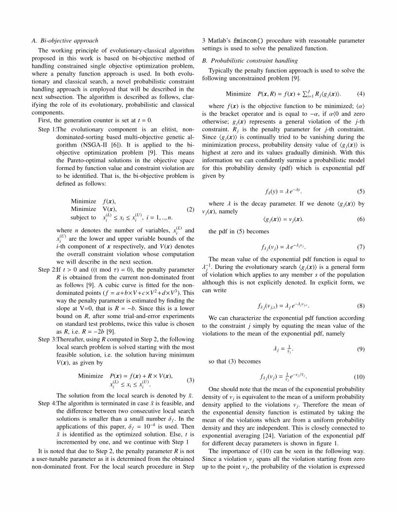
One should note that the mean of the exponential probabilitydensity of v j is equivalent to the mean of a uniform probabilitydensity applied to the violations v j. Therefore the mean ofthe exponential density function is estimated by taking themean of the violations which are from a uniform probabilitydensity and they are independent. This is closely connected toexponential averaging [24]. Variation of the exponential pdffor different decay parameters is shown in figure 1.

The importance of (10) can be seen in the following way.Since a violation v j spans all the violation starting from zeroup to the point v j, the probability of the violation is expressed

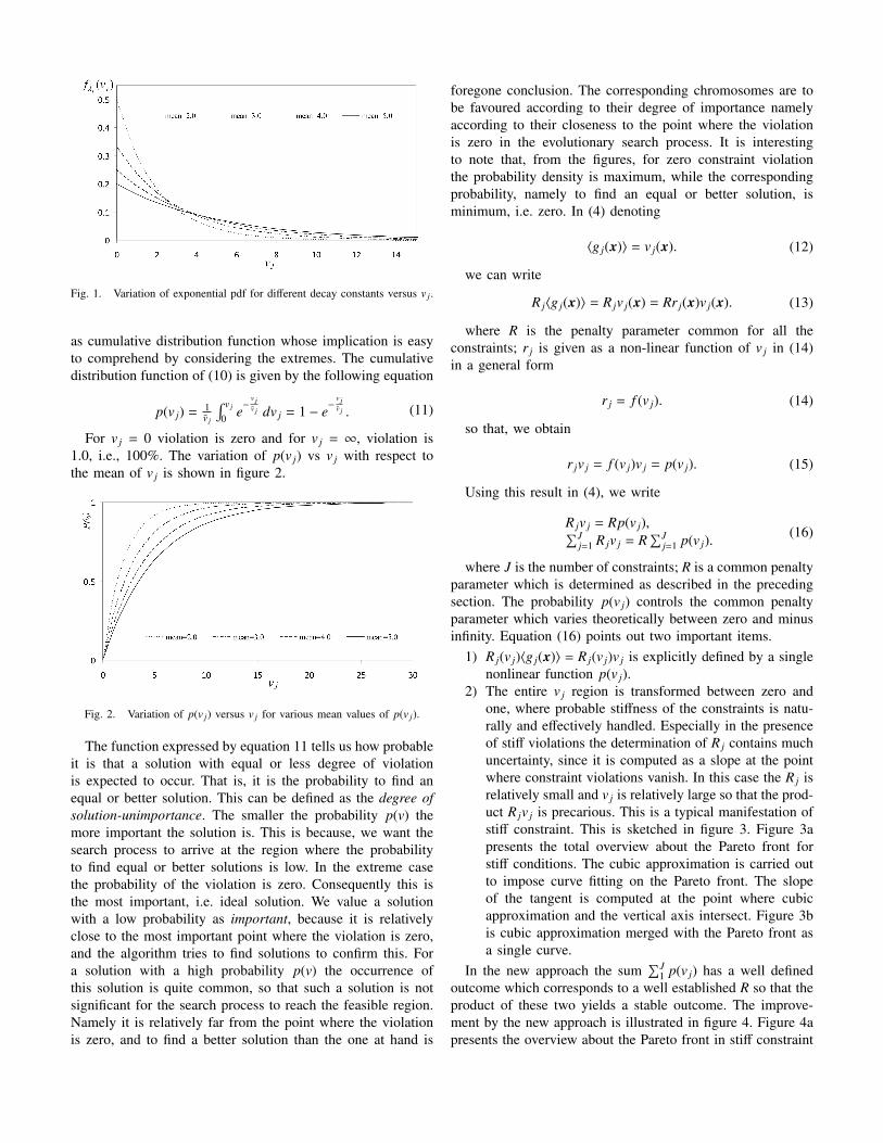
Fig. 1. Variation of exponential pdf for different decay constants versus v j.

as cumulative distribution function whose implication is easyto comprehend by considering the extremes. The cumulativedistribution function of (10) is given by the following equation

p(v j) = 1v j

∫ v j

0 e−

v jv j dv j = 1 − e

−v jv j . (11)

For v j = 0 violation is zero and for v j = ∞, violation is1.0, i.e., 100%. The variation of p(v j) vs v j with respect tothe mean of v j is shown in figure 2.

Fig. 2. Variation of p(v j) versus v j for various mean values of p(v j).

The function expressed by equation 11 tells us how probableit is that a solution with equal or less degree of violationis expected to occur. That is, it is the probability to find anequal or better solution. This can be defined as the degree ofsolution-unimportance. The smaller the probability p(v) themore important the solution is. This is because, we want thesearch process to arrive at the region where the probabilityto find equal or better solutions is low. In the extreme casethe probability of the violation is zero. Consequently this isthe most important, i.e. ideal solution. We value a solutionwith a low probability as important, because it is relativelyclose to the most important point where the violation is zero,and the algorithm tries to find solutions to confirm this. Fora solution with a high probability p(v) the occurrence ofthis solution is quite common, so that such a solution is notsignificant for the search process to reach the feasible region.Namely it is relatively far from the point where the violationis zero, and to find a better solution than the one at hand is

foregone conclusion. The corresponding chromosomes are tobe favoured according to their degree of importance namelyaccording to their closeness to the point where the violationis zero in the evolutionary search process. It is interestingto note that, from the figures, for zero constraint violationthe probability density is maximum, while the correspondingprobability, namely to find an equal or better solution, isminimum, i.e. zero. In (4) denoting

〈g j(x)〉 = v j(x). (12)

we can write

R j〈g j(x)〉 = R jv j(x) = Rr j(x)v j(x). (13)

where R is the penalty parameter common for all theconstraints; r j is given as a non-linear function of v j in (14)in a general form

r j = f (v j). (14)

so that, we obtain

r jv j = f (v j)v j = p(v j). (15)

Using this result in (4), we write

R jv j = Rp(v j),∑Jj=1 R jv j = R

∑Jj=1 p(v j).

(16)

where J is the number of constraints; R is a common penaltyparameter which is determined as described in the precedingsection. The probability p(v j) controls the common penaltyparameter which varies theoretically between zero and minusinfinity. Equation (16) points out two important items.

1) R j(v j)〈g j(x)〉 = R j(v j)v j is explicitly defined by a singlenonlinear function p(v j).

2) The entire v j region is transformed between zero andone, where probable stiffness of the constraints is natu-rally and effectively handled. Especially in the presenceof stiff violations the determination of R j contains muchuncertainty, since it is computed as a slope at the pointwhere constraint violations vanish. In this case the R j isrelatively small and v j is relatively large so that the prod-uct R jv j is precarious. This is a typical manifestation ofstiff constraint. This is sketched in figure 3. Figure 3apresents the total overview about the Pareto front forstiff conditions. The cubic approximation is carried outto impose curve fitting on the Pareto front. The slopeof the tangent is computed at the point where cubicapproximation and the vertical axis intersect. Figure 3bis cubic approximation merged with the Pareto front asa single curve.

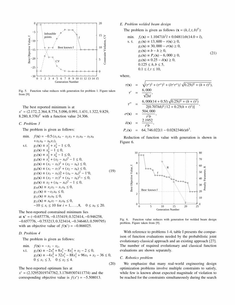
In the new approach the sum∑J

1 p(v j) has a well definedoutcome which corresponds to a well established R so that theproduct of these two yields a stable outcome. The improve-ment by the new approach is illustrated in figure 4. Figure 4apresents the overview about the Pareto front in stiff constraint

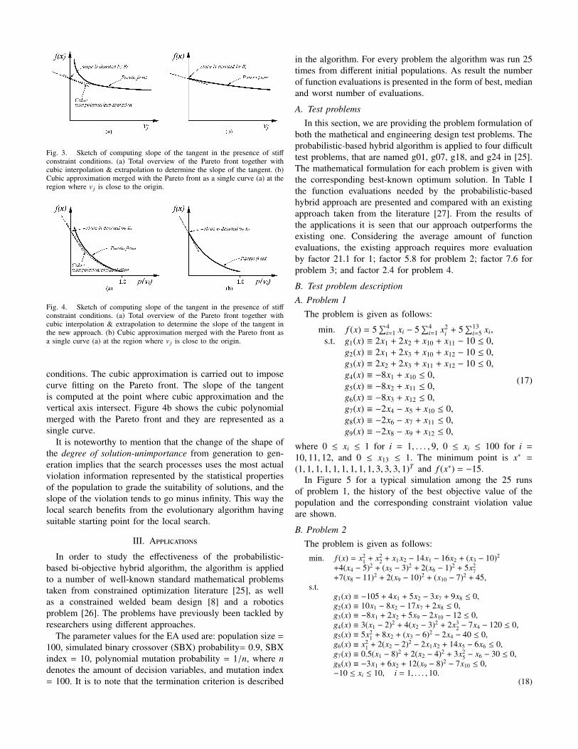
Fig. 3. Sketch of computing slope of the tangent in the presence of stiffconstraint conditions. (a) Total overview of the Pareto front together withcubic interpolation & extrapolation to determine the slope of the tangent. (b)Cubic approximation merged with the Pareto front as a single curve (a) at theregion where v j is close to the origin.

Fig. 4. Sketch of computing slope of the tangent in the presence of stiffconstraint conditions. (a) Total overview of the Pareto front together withcubic interpolation & extrapolation to determine the slope of the tangent inthe new approach. (b) Cubic approximation merged with the Pareto front asa single curve (a) at the region where v j is close to the origin.

conditions. The cubic approximation is carried out to imposecurve fitting on the Pareto front. The slope of the tangentis computed at the point where cubic approximation and thevertical axis intersect. Figure 4b shows the cubic polynomialmerged with the Pareto front and they are represented as asingle curve.

It is noteworthy to mention that the change of the shape ofthe degree of solution-unimportance from generation to gen-eration implies that the search processes uses the most actualviolation information represented by the statistical propertiesof the population to grade the suitability of solutions, and theslope of the violation tends to go minus infinity. This way thelocal search benefits from the evolutionary algorithm havingsuitable starting point for the local search.

III. Applications

In order to study the effectiveness of the probabilistic-based bi-objective hybrid algorithm, the algorithm is appliedto a number of well-known standard mathematical problemstaken from constrained optimization literature [25], as wellas a constrained welded beam design [8] and a roboticsproblem [26]. The problems have previously been tackled byresearchers using different approaches.

The parameter values for the EA used are: population size =

100, simulated binary crossover (SBX) probability= 0.9, SBXindex = 10, polynomial mutation probability = 1/n, where ndenotes the amount of decision variables, and mutation index= 100. It is to note that the termination criterion is described

in the algorithm. For every problem the algorithm was run 25times from different initial populations. As result the numberof function evaluations is presented in the form of best, medianand worst number of evaluations.

A. Test problemsIn this section, we are providing the problem formulation of

both the mathetical and engineering design test problems. Theprobabilistic-based hybrid algorithm is applied to four difficulttest problems, that are named g01, g07, g18, and g24 in [25].The mathematical formulation for each problem is given withthe corresponding best-known optimum solution. In Table Ithe function evaluations needed by the probabilistic-basedhybrid approach are presented and compared with an existingapproach taken from the literature [27]. From the results ofthe applications it is seen that our approach outperforms theexisting one. Considering the average amount of functionevaluations, the existing approach requires more evaluationby factor 21.1 for 1; factor 5.8 for problem 2; factor 7.6 forproblem 3; and factor 2.4 for problem 4.

B. Test problem descriptionA. Problem 1

The problem is given as follows:

min. f (x) = 5∑4

i=1 xi − 5∑4

i=1 x2i + 5

∑13i=5 xi,

s.t. g1(x) ≡ 2x1 + 2x2 + x10 + x11 − 10 ≤ 0,g2(x) ≡ 2x1 + 2x3 + x10 + x12 − 10 ≤ 0,g3(x) ≡ 2x2 + 2x3 + x11 + x12 − 10 ≤ 0,g4(x) ≡ −8x1 + x10 ≤ 0,g5(x) ≡ −8x2 + x11 ≤ 0,g6(x) ≡ −8x3 + x12 ≤ 0,g7(x) ≡ −2x4 − x5 + x10 ≤ 0,g8(x) ≡ −2x6 − x7 + x11 ≤ 0,g9(x) ≡ −2x8 − x9 + x12 ≤ 0,

(17)

where 0 ≤ xi ≤ 1 for i = 1, . . . , 9, 0 ≤ xi ≤ 100 for i =

10, 11, 12, and 0 ≤ x13 ≤ 1. The minimum point is x∗ =

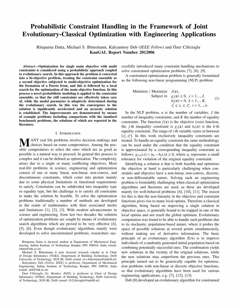
(1, 1, 1, 1, 1, 1, 1, 1, 1, 3, 3, 3, 1)T and f (x∗) = −15.In Figure 5 for a typical simulation among the 25 runs

of problem 1, the history of the best objective value of thepopulation and the corresponding constraint violation valueare shown.

B. Problem 2The problem is given as follows:

min. f (x) = x21 + x2

2 + x1 x2 − 14x1 − 16x2 + (x3 − 10)2

+4(x4 − 5)2 + (x5 − 3)2 + 2(x6 − 1)2 + 5x27

+7(x8 − 11)2 + 2(x9 − 10)2 + (x10 − 7)2 + 45,s.t.

g1(x) ≡ −105 + 4x1 + 5x2 − 3x7 + 9x8 ≤ 0,g2(x) ≡ 10x1 − 8x2 − 17x7 + 2x8 ≤ 0,g3(x) ≡ −8x1 + 2x2 + 5x9 − 2x10 − 12 ≤ 0,g4(x) ≡ 3(x1 − 2)2 + 4(x2 − 3)2 + 2x3

2 − 7x4 − 120 ≤ 0,g5(x) ≡ 5x2

1 + 8x2 + (x3 − 6)2 − 2x4 − 40 ≤ 0,g6(x) ≡ x2

1 + 2(x2 − 2)2 − 2x1 x2 + 14x5 − 6x6 ≤ 0,g7(x) ≡ 0.5(x1 − 8)2 + 2(x2 − 4)2 + 3x2

5 − x6 − 30 ≤ 0,g8(x) ≡ −3x1 + 6x2 + 12(x9 − 8)2 − 7x10 ≤ 0,−10 ≤ xi ≤ 10, i = 1, . . . , 10.

(18)

Serial and Parallel Robot Manipulators: Kinematic Dynamics and Control 11

Best known f

pointsInfeasible

CV

f

8 9 10 11 12 13 14 15

0

5

10

20

Bes

t Obj

ectiv

e V

alue

, f

Con

stra

int V

iola

tion,

CV

Generation Number

15

−30

−25

−20

−15

−10

−5

0

0 1 2 3 4 5 6 7

Fig. 4. Function value reduces with gen-eration for g01 problem. Figure takenfrom [15].

f

R

Best−known f

0

8

10

0 5 10 15 20 25 0

10

20

30

40

50

60

70

80

Bes

t Obj

ectiv

e V

alue

, f

Pen

alty

Par

amet

er, R

Generation Number

4

2

6

Fig. 5. Function value reduces with gen-eration for welded beam design problem.Figure taken from [15].

Table 1. Comparison of function evaluations needed by the fuzzy-based hybrid ap-proach and an existing approach [27]; the number of required evolutionary and classicalevaluations are shown separately.

Problem Best known Function Evaluations (FEs)optima Zavala, Aguirre & Proposed Hybrid Approach(f∗) Diharce [27]

Mathematical Best Median Worst Best Median Worstg01 −15.0 80,776 90,343 96,669 1,475 4,274 22,367

NSGA-II+Local 1,000+475 3,500+774 14,000+8,367g07 24.306209 1,14,709 1,38,767 2,08,751 4,069 23,842 55,721

NSGA-II+Local 2,400+1,669 14,400+9,442 34,400+21,321g18 −0.866025 97,157 1,07,690 1,24,217 2,107 14,082 36,547

NSGA-II+Local 1,000+1,107 9,000+5,082 19,000+17,547g24 −5.508013 11,081 18,278 6,33,378 1,263 7,695 41,762

NSGA-II+Local 1,000+263 6,500+1,195 39,9000+2,762

Engineering Approach [8] Proposed Hybrid ApproachWelded beam design 2.38119 3,20,000 3,20,000 3,20,000 2,778 21,287 44,617

NSGA-II+Local 1,500+1,278 18,000+3,287 37,000+7,617

violation to be reached for the constraints simultanously during the search pro-cess. Therefore the proposed fuzzy based methodology is also applied to a con-strained robotics problem. The problem concerns the design of a robot gripper,which is is commonly used in industry. The vector of seven design variables arex = (a, b, c, e, f, l, δ)T , where a, b, c, e, f, l are dimensions (link lengths) ofthe gripper and δ is the angle between elements b and c (Figure 3.2): [28]

The objective is to minimize the difference between maximium and minimumforce in the gripper. That is, the problem is Minimize

f1(x) = maxz

Fk(x, z)−minz

Fk(x, z). (8)

The minimization is subject to the following geometric and force constraints:

Fig. 5. Function value reduces with generation for problem 1. Figure takenfrom [9].

The best reported minimum is atx∗ = (2.172, 2.364, 8.774, 5.096, 0.991, 1.431, 1.322, 9.829,8.280, 8.376)T with a function value 24.306.

C. Problem 3

The problem is given as follows:

min. f (x) = −0.5 (x1x4 − x2x3 + x3x9 − x5x9+x5x8 − x6x7),

s.t. g1(x) ≡ x23 + x2

4 − 1 ≤ 0,g2(x) ≡ x2

9 − 1 ≤ 0,g3(x) ≡ x2

5 + x26 − 1 ≤ 0,

g4(x) ≡ x21 + (x2 − x9)2 − 1 ≤ 0,

g5(x) ≡ (x1 − x5)2 + (x2 − x6) ≤ 0,g6(x) ≡ (x1 − x7)2 + (x2 − x8) ≤ 0,g7(x) ≡ (x3 − x5)2 + (x4 − x6)2 − 1‘0,g8(x) ≡ (x3 − x7)2 + (x4 − x8)2− ≤ 0,g9(x) ≡ x2 + (x8 − x9)2 − 1 ≤ 0,g10(x) ≡ x2x3 − x1x4 ≤ 0,g11(x) ≡ −x3x9 ≤ 0,g12(x) ≡ x5x9 ≤ 0,g13(x) ≡ x6x7 − x5x8 ≤ 0,−10 ≤ xi ≤ 10 for i = 1, . . . , 8, 0 ≤ x9 ≤ 20.

(19)

The best-reported constrained minimum liesat x∗ = (−0.657776,−0.153419, 0.323414,−0.946258,−0.657776,−0.753213, 0.323414,−0.346463, 0.599795)with an objective value of f (x∗) = −0.866025.

D. Problem 4

The problem is given as follows:

min. f (x) = −x1 − x2,s.t. g1(x) ≡ −2x4

1 + 8x31 − 8x2

1 + x2 − 2 ≤ 0,g2(x) ≡ −4x4

1 + 32x31 − 88x2

1 + 96x1 + x2 − 36 ≤ 0,0 ≤ x1 ≤ 3, 0 ≤ x2 ≤ 4.

(20)The best-reported optimum lies atx∗ = (2.32952019747762, 3.17849307411774) and thecorresponding objective value is f (x∗) = −5.508013.

E. Problem welded beam design

The problem is given as follows (x = (h, l, t, b)T ):

min. f1(x) = 1.10471h2l + 0.04811tb(14.0 + l),s. t. g1(x) ≡ 13, 600 − τ(x) ≥ 0,

g2(x) ≡ 30, 000 − σ(x) ≥ 0,g3(x) ≡ b − h ≥ 0,g4(x) ≡ Pc(x) − 6, 000 ≥ 0,g5(x) ≡ 0.25 − δ(x) ≥ 0,0.125 ≤ h, b ≤ 5,0.1 ≤ l, t ≤ 10,

(21)

where,

τ(x) =

√(τ′)2 + (τ′′)2 + (lτ′τ′′)/

√0.25(l2 + (h + t)2),

τ′ =6, 000√

2hl,

τ′′ =6, 000(14 + 0.5l)

√0.25(l2 + (h + t)2)

2[0.707hl(l2/12 + 0.25(h + t)2)],

σ(x) =504, 000

t2b,

δ(x) =2.1952

t3b,

Pc(x) = 64, 746.022(1 − 0.0282346t)tb3.

Reduction of function value with generation is shown inFigure 6.Serial and Parallel Robot Manipulators: Kinematic Dynamics and Control 11

Best known f

pointsInfeasible

CV

f

8 9 10 11 12 13 14 15

0

5

10

20

Bes

t Obj

ectiv

e V

alue

, f

Con

stra

int V

iola

tion,

CV

Generation Number

15

−30

−25

−20

−15

−10

−5

0

0 1 2 3 4 5 6 7

Fig. 4. Function value reduces with gen-eration for g01 problem. Figure takenfrom [15].

f

R

Best−known f

0

8

10

0 5 10 15 20 25 0

10

20

30

40

50

60

70

80

Bes

t Obj

ectiv

e V

alue

, f

Pen

alty

Par

amet

er, R

Generation Number

4

2

6

Fig. 5. Function value reduces with gen-eration for welded beam design problem.Figure taken from [15].

Table 1. Comparison of function evaluations needed by the fuzzy-based hybrid ap-proach and an existing approach [27]; the number of required evolutionary and classicalevaluations are shown separately.

Problem Best known Function Evaluations (FEs)optima Zavala, Aguirre & Proposed Hybrid Approach(f∗) Diharce [27]

Mathematical Best Median Worst Best Median Worstg01 −15.0 80,776 90,343 96,669 1,475 4,274 22,367

NSGA-II+Local 1,000+475 3,500+774 14,000+8,367g07 24.306209 1,14,709 1,38,767 2,08,751 4,069 23,842 55,721

NSGA-II+Local 2,400+1,669 14,400+9,442 34,400+21,321g18 −0.866025 97,157 1,07,690 1,24,217 2,107 14,082 36,547

NSGA-II+Local 1,000+1,107 9,000+5,082 19,000+17,547g24 −5.508013 11,081 18,278 6,33,378 1,263 7,695 41,762

NSGA-II+Local 1,000+263 6,500+1,195 39,9000+2,762

Engineering Approach [8] Proposed Hybrid ApproachWelded beam design 2.38119 3,20,000 3,20,000 3,20,000 2,778 21,287 44,617

NSGA-II+Local 1,500+1,278 18,000+3,287 37,000+7,617

violation to be reached for the constraints simultanously during the search pro-cess. Therefore the proposed fuzzy based methodology is also applied to a con-strained robotics problem. The problem concerns the design of a robot gripper,which is is commonly used in industry. The vector of seven design variables arex = (a, b, c, e, f, l, δ)T , where a, b, c, e, f, l are dimensions (link lengths) ofthe gripper and δ is the angle between elements b and c (Figure 3.2): [28]

The objective is to minimize the difference between maximium and minimumforce in the gripper. That is, the problem is Minimize

f1(x) = maxz

Fk(x, z)−minz

Fk(x, z). (8)

The minimization is subject to the following geometric and force constraints:

Fig. 6. Function value reduces with generation for welded beam designproblem. Figure taken from [9].

With reference to problems 1-4, table I presents the compar-ison of function evaluations needed by the probabilistic jointevolutionary-classical approach and an existing approach [27].The number of required evolutionary and classical functionevaluations are shown separately.

C. Robotics problem

We emphasize that many real-world engineering designoptimization problems involve multiple constraints to satisfy,while few is known about expected magnitude of violation tobe reached for the constraints simultaneously during the search

TABLE IComparison of function evaluations needed by the probabilistic hybrid approach and an existing approach [27]; the number of required evolutionary and

classical evaluations are shown separately.

Problem Best known Function Evaluations (FEs)optima Zavala, Aguirre & Proposed Hybrid Approach

( f ∗) Diharce [27]Mathematical Best Median Worst Best Median Worst

Problem 1 −15.0 80,776 90,343 96,669 1,475 4,274 22,367NSGA-II+Local 1,000+475 3,500+774 14,000+8,367

Problem 2 24.306209 1,14,709 1,38,767 2,08,751 4,069 23,842 55,721NSGA-II+Local 2,400+1,669 14,400+9,442 34,400+21,321

Problem 3 −0.866025 97,157 1,07,690 1,24,217 2,107 14,082 36,547NSGA-II+Local 1,000+1,107 9,000+5,082 19,000+17,547

Problem 4 −5.508013 11,081 18,278 6,33,378 1,263 7,695 41,762NSGA-II+Local 1,000+263 6,500+1,195 39,000+2,762

Engineering Approach [8] Proposed Hybrid ApproachWelded beam design 2.38119 3,20,000 3,20,000 3,20,000 2,778 21,287 44,617

NSGA-II+Local 1,500+1,278 18,000+3,287 37,000+7,617

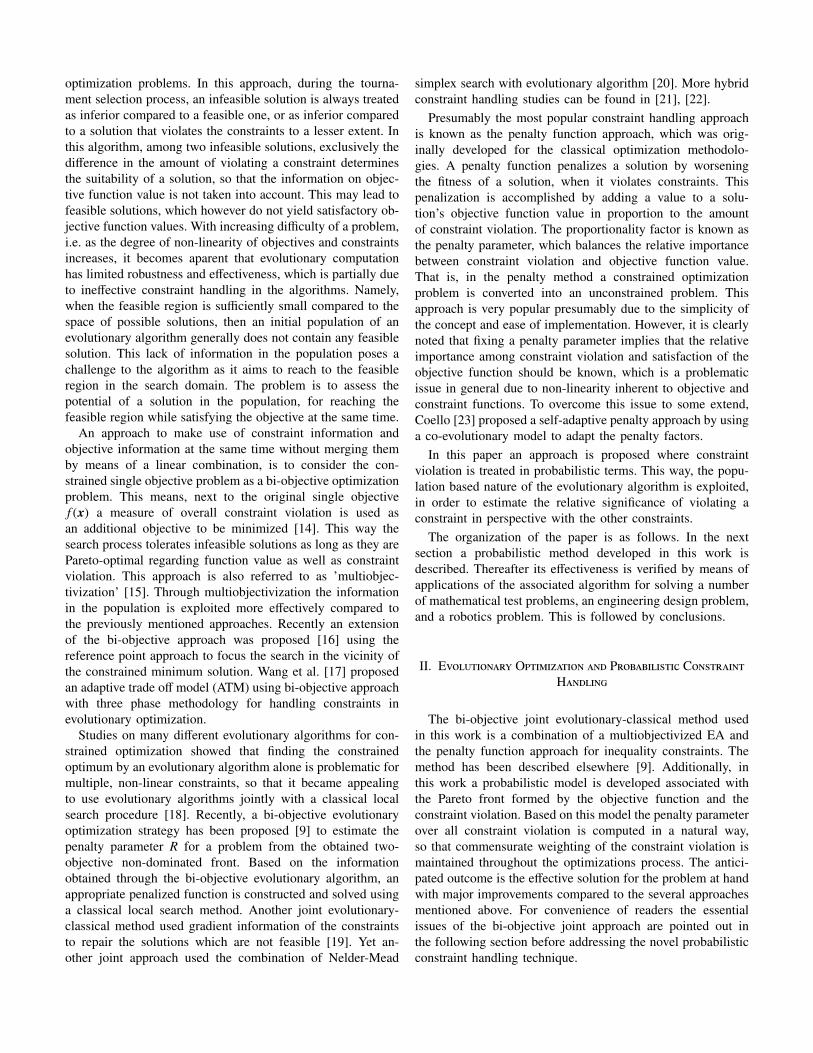
process. Therefore proposed probabilistic based methodologyis also applied to a constrained robot gripper design optimiza-tion problem. The problem concerns the design of a robotgripper optimally, which is commonly used in industry asan interaction device between environment, to pick and placeobject and to perform grasping and manipulation tasks. Thevector of seven design variables are x = (a, b, c, e, f , l, δ)T ,where a, b, c, e, f , l are dimensions (link lengths) of the robotgripper and δ is the angle between link length b with c shownin figure 7 [26].12 R. Datta, M.S. Bittermann, K. Deb, I.S. Sariyildiz

y

cbz a

f

l

eβ

α

δ

Fk

Fk

Fig. 6. A sketch of robot Gripper-I. Figure taken from [28]

g1(x) ≡ Ymin − y(x, Zmax) ≥ 0,g2(x) ≡ y(x, Zmax) ≥ 0,g3(x) ≡ y(x, 0)− Ymax ≥ 0,g4(x) ≡ YG − y(x, 0) ≥ 0,g5(x) ≡ (a+ b)2 − l2 − e2 ≥ 0.g6(x) ≡ (l − Zmax)

2 + (a− e)2 − b2 ≥ 0,g7(x) ≡ l − Zmax ≥ 0.

(9)

where,g ≡

√(l − z)2 + e2,

b2 ≡ a2 + g2 − 2.a.g. cos(α− φ),

α ≡ arccos(a2+g2−b2

2.a.g ) + φ,

a2 ≡ b2 + g2 − 2.b.g. cos(β + φ),

β ≡ arccos( b2+g2−a2

2.b.g )− φ,

φ ≡ arctan( el−z ),

Fk ≡ P.b sin(α+β)2.c cosα ,

y(x, z) ≡ 2(e+ f + csin(β + δ)),10 ≤ a ≤ 250,10 ≤ b ≤ 250,100 ≤ c ≤ 300,0 ≤ e ≤ 50,10 ≤ f ≤ 250,100 ≤ l ≤ 300,1.0 ≤ δ ≤ 3.14,Ymin = 50mm,Ymax = 100mm,YG = 150mm,Zmax = 50mm,P = 100N,FG = 50N.

(10)

Fig. 7. A sketch of robot Gripper-I. Figure taken from [26]

The objective is to minimize the difference between maxi-mum and minimum force in the gripper. Minimize

f (x) = maxz

Fk(x, z) −minz

Fk(x, z). (22)

The minimization of robot gripper design is subject to thefollowing geometric and force constraints:

g1(x) ≡ Ymin − y(x,Zmax) ≥ 0,g2(x) ≡ y(x,Zmax) ≥ 0,g3(x) ≡ y(x, 0) − Ymax ≥ 0,g4(x) ≡ YG − y(x, 0) ≥ 0,g5(x) ≡ (a + b)2 − l2 − e2 ≥ 0.g6(x) ≡ (l − Zmax)2 + (a − e)2 − b2 ≥ 0,g7(x) ≡ l − Zmax ≥ 0.

(23)

where,

g ≡√

(l − z)2 + e2,

b2 ≡ a2 + g2 − 2.a.g. cos(α − φ),

α ≡ arccos(a2 + g2 − b2

2.a.g) + φ,

a2 ≡ b2 + g2 − 2.b.g. cos(β + φ),

β ≡ arccos(b2 + g2 − a2

2.b.g) − φ,

φ ≡ arctan(e

l − z),

Fk ≡P.b sin(α + β)

2.c cosα,

y(x, z) ≡ 2(e + f + csin(β + δ)),

10 ≤ a ≤ 250,10 ≤ b ≤ 250,100 ≤ c ≤ 300,0 ≤ e ≤ 50,10 ≤ f ≤ 250,100 ≤ l ≤ 300,1.0 ≤ δ ≤ 3.14,

Ymin = 50 mm,Ymax = 100 mm,YG = 150 mm,Zmax = 50 mm,P = 100 N,FG = 50 N.

(24)

Table II shows the best, median and worst objective func-tion values obtained using probabilistic constraint handlingmethodology and compared with an existing approach takenfrom literature [26]. It is noted that due to the multi-modalityof the robotics problems at hand the algorithm is executedwithout local search component involved in order to ensurerobustness of the algorithm. Despite this, as for the mathe-matical problems, also for the robotics problems the prob-

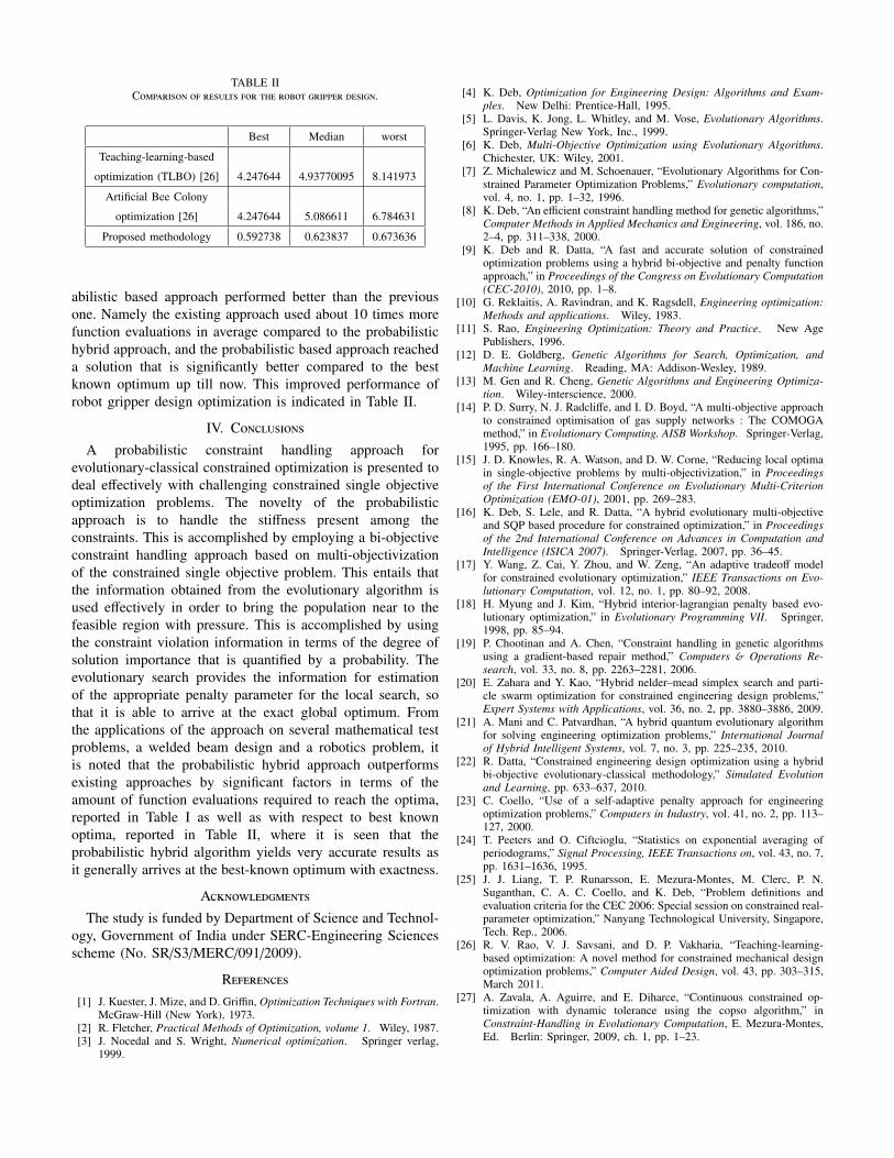
TABLE IIComparison of results for the robot gripper design.

Best Median worst

Teaching-learning-based

optimization (TLBO) [26] 4.247644 4.93770095 8.141973

Artificial Bee Colony

optimization [26] 4.247644 5.086611 6.784631

Proposed methodology 0.592738 0.623837 0.673636

abilistic based approach performed better than the previousone. Namely the existing approach used about 10 times morefunction evaluations in average compared to the probabilistichybrid approach, and the probabilistic based approach reacheda solution that is significantly better compared to the bestknown optimum up till now. This improved performance ofrobot gripper design optimization is indicated in Table II.

IV. ConclusionsA probabilistic constraint handling approach for

evolutionary-classical constrained optimization is presented todeal effectively with challenging constrained single objectiveoptimization problems. The novelty of the probabilisticapproach is to handle the stiffness present among theconstraints. This is accomplished by employing a bi-objectiveconstraint handling approach based on multi-objectivizationof the constrained single objective problem. This entails thatthe information obtained from the evolutionary algorithm isused effectively in order to bring the population near to thefeasible region with pressure. This is accomplished by usingthe constraint violation information in terms of the degree ofsolution importance that is quantified by a probability. Theevolutionary search provides the information for estimationof the appropriate penalty parameter for the local search, sothat it is able to arrive at the exact global optimum. Fromthe applications of the approach on several mathematical testproblems, a welded beam design and a robotics problem, itis noted that the probabilistic hybrid approach outperformsexisting approaches by significant factors in terms of theamount of function evaluations required to reach the optima,reported in Table I as well as with respect to best knownoptima, reported in Table II, where it is seen that theprobabilistic hybrid algorithm yields very accurate results asit generally arrives at the best-known optimum with exactness.

AcknowledgmentsThe study is funded by Department of Science and Technol-

ogy, Government of India under SERC-Engineering Sciencesscheme (No. SR/S3/MERC/091/2009).

References[1] J. Kuester, J. Mize, and D. Griffin, Optimization Techniques with Fortran.

McGraw-Hill (New York), 1973.[2] R. Fletcher, Practical Methods of Optimization, volume 1. Wiley, 1987.[3] J. Nocedal and S. Wright, Numerical optimization. Springer verlag,

1999.

[4] K. Deb, Optimization for Engineering Design: Algorithms and Exam-ples. New Delhi: Prentice-Hall, 1995.

[5] L. Davis, K. Jong, L. Whitley, and M. Vose, Evolutionary Algorithms.Springer-Verlag New York, Inc., 1999.

[6] K. Deb, Multi-Objective Optimization using Evolutionary Algorithms.Chichester, UK: Wiley, 2001.

[7] Z. Michalewicz and M. Schoenauer, “Evolutionary Algorithms for Con-strained Parameter Optimization Problems,” Evolutionary computation,vol. 4, no. 1, pp. 1–32, 1996.

[8] K. Deb, “An efficient constraint handling method for genetic algorithms,”Computer Methods in Applied Mechanics and Engineering, vol. 186, no.2–4, pp. 311–338, 2000.

[9] K. Deb and R. Datta, “A fast and accurate solution of constrainedoptimization problems using a hybrid bi-objective and penalty functionapproach,” in Proceedings of the Congress on Evolutionary Computation(CEC-2010), 2010, pp. 1–8.

[10] G. Reklaitis, A. Ravindran, and K. Ragsdell, Engineering optimization:Methods and applications. Wiley, 1983.

[11] S. Rao, Engineering Optimization: Theory and Practice. New AgePublishers, 1996.

[12] D. E. Goldberg, Genetic Algorithms for Search, Optimization, andMachine Learning. Reading, MA: Addison-Wesley, 1989.

[13] M. Gen and R. Cheng, Genetic Algorithms and Engineering Optimiza-tion. Wiley-interscience, 2000.

[14] P. D. Surry, N. J. Radcliffe, and I. D. Boyd, “A multi-objective approachto constrained optimisation of gas supply networks : The COMOGAmethod,” in Evolutionary Computing. AISB Workshop. Springer-Verlag,1995, pp. 166–180.

[15] J. D. Knowles, R. A. Watson, and D. W. Corne, “Reducing local optimain single-objective problems by multi-objectivization,” in Proceedingsof the First International Conference on Evolutionary Multi-CriterionOptimization (EMO-01), 2001, pp. 269–283.

[16] K. Deb, S. Lele, and R. Datta, “A hybrid evolutionary multi-objectiveand SQP based procedure for constrained optimization,” in Proceedingsof the 2nd International Conference on Advances in Computation andIntelligence (ISICA 2007). Springer-Verlag, 2007, pp. 36–45.

[17] Y. Wang, Z. Cai, Y. Zhou, and W. Zeng, “An adaptive tradeoff modelfor constrained evolutionary optimization,” IEEE Transactions on Evo-lutionary Computation, vol. 12, no. 1, pp. 80–92, 2008.

[18] H. Myung and J. Kim, “Hybrid interior-lagrangian penalty based evo-lutionary optimization,” in Evolutionary Programming VII. Springer,1998, pp. 85–94.

[19] P. Chootinan and A. Chen, “Constraint handling in genetic algorithmsusing a gradient-based repair method,” Computers & Operations Re-search, vol. 33, no. 8, pp. 2263–2281, 2006.

[20] E. Zahara and Y. Kao, “Hybrid nelder–mead simplex search and parti-cle swarm optimization for constrained engineering design problems,”Expert Systems with Applications, vol. 36, no. 2, pp. 3880–3886, 2009.

[21] A. Mani and C. Patvardhan, “A hybrid quantum evolutionary algorithmfor solving engineering optimization problems,” International Journalof Hybrid Intelligent Systems, vol. 7, no. 3, pp. 225–235, 2010.

[22] R. Datta, “Constrained engineering design optimization using a hybridbi-objective evolutionary-classical methodology,” Simulated Evolutionand Learning, pp. 633–637, 2010.

[23] C. Coello, “Use of a self-adaptive penalty approach for engineeringoptimization problems,” Computers in Industry, vol. 41, no. 2, pp. 113–127, 2000.

[24] T. Peeters and O. Ciftcioglu, “Statistics on exponential averaging ofperiodograms,” Signal Processing, IEEE Transactions on, vol. 43, no. 7,pp. 1631–1636, 1995.

[25] J. J. Liang, T. P. Runarsson, E. Mezura-Montes, M. Clerc, P. N.Suganthan, C. A. C. Coello, and K. Deb, “Problem definitions andevaluation criteria for the CEC 2006: Special session on constrained real-parameter optimization,” Nanyang Technological University, Singapore,Tech. Rep., 2006.

[26] R. V. Rao, V. J. Savsani, and D. P. Vakharia, “Teaching-learning-based optimization: A novel method for constrained mechanical designoptimization problems,” Computer Aided Design, vol. 43, pp. 303–315,March 2011.

[27] A. Zavala, A. Aguirre, and E. Diharce, “Continuous constrained op-timization with dynamic tolerance using the copso algorithm,” inConstraint-Handling in Evolutionary Computation, E. Mezura-Montes,Ed. Berlin: Springer, 2009, ch. 1, pp. 1–23.