Probabilistic Development Factor Models with Applications to

Loss Reserve Variability, Prediction Intervals, and

Risk Based Capital

by Ben Zehnwirth

447

1.0 INTRODUCTION AND SUMMARY

The present paper aims to present a statistical modelling framework and environment

for conducting loss reserving analysis. The modelling framework and approach

affords numerous advantages including increased accuracy of estimates and

modelling of loss reserve variability. Since the loss reserve is likely to be the largest

item in the insurer's balance sheet and is subject to much uncertainty, modelling of

loss reserve variability is an integral component of assessing insurer solvency and

assessment of risk based capital.

The paper is organised as follows:

Forecasting and some modelling concepts are introduced in Section 2. The salient

features of the data that ought to be captured by a model are discussed and

arguments in favour of probabilistic models are presented. It is emphasised that the

only way to assess loss reserve variability is through probabilistic models. The

statistic~ MODELLING FRAMEWORK is introduced where each model in the

framework has four components of interest. The first three involve trends in the three

directions, development year, payment~calendar year and accident year and the

fourth component is the random fluctuations (distributions) about the trends.

In Section 3 we begin by discussing trend adjustments to a univariate time series and

illustrate how analogous adjustments to loss reserving data cannot be handled by

graph and ruler, mainly as a consequence of the projection of the payment/calendar

year trends onto the development year and accident year directions. Two

deterministic, models Cape Cod (CC) and Cape Cod with constant inflation (CCI) are

discussed. Age-to-age development factors are defined as trend parameters.

A rich class of deterministic development factor models is introduced in Section 4

where each model in the framework contains the three trend components of interest.

It is shown how as a result of the projection of calender year (trends), a very simple

448

trend model causes very different development year trends (development factors) for

different accident years. Standard actuarial techniques based on age-to-age link

ratios of the cumulative payments cannot capture the payment/calendar year trends

in the payments.

In Section 5 the class (or family) of deterministic development factor models that only

contain trend components in the three directions is extended to include random

fluctuations. The resulting models in the rich Development Factor Family (DFF) are

probabilistic models that relate the distributions of 'payments' in the various cells in

the triangle by trend parameters. It is emphasised that one of the principal uses of

regression is the estimation (or fitting) of distributions. Estimation of a model

belonging to the DFF involves the fitting of distributions to the cells in the loss

development array. Data based on a simple DFF model are generated (simulated)

and it is demonstrated how the development year patterns are invariably complex.

The trends cannot be determined from the age-to-age link ratios nor from graphs.

For readers who are sceptics and may argue "But this is simulated data" should read

Section 1 2 where we analyse real life data involving a line written by a larger insurer

for which the age-to-age link ratios on the cumulative payments are relatively smooth.

HOWEVER, there are major shifts in payment~calendar year trends in the payments

that are quite alarming.

We use regression for a number of purposes:

Estimation of trends.

Estimation or fitting of distributions.

In Section 6 we demonstrate how regression can also be employed to adjust data for

trends. We state as a THEOREM that the only way to separate payment/calendar

year trends from development year trends is by application of regression. Practical

applications of regressions involving real life data sets are given in Sections 12 and

13.

In Section 6 we also present a number of tests that we believe any sound loss

449

reserving statistical framework should pass. It is shown that standard actuarial

techniques based on age-to-age link ratios fail these minimum tests.

As a result of the dependence of the payment/calendar year direction on the other

two directions, many of the models in the DFF that contain many parameters cannot

be estimated in a spreadsheet or statistical package and some that can be estimated

may contain much parameter uncertainty. This phenomenon, known as

multicollinear'ity, is discussed in Section 7 and motivates the introduction of varying

parameter, dynamic or credibility models. Varying parameters or stochastic

parameters can also be regarded as proxies for the myriad of variables that affect the

complex claims generating process.

In Section 8 we show how the (fixed) parameter regression models may be estimated

in a spreadsheet or statistical package and how an estimated model may be

employed in producing forecast distributions of (incremental) payments. The forecast

(estimated) distributions provide information required for the assessment of risk based

capital and solvency.

Additional modelling concepts including parsimony, Akaike Information Criterion and

distributional assumptions are discussed in Section 9. Moreover, we describe the

importance of the twin concepts of stability and validation analysis and show how

data with unstable trends (in the payments) are less predictable (subject to greater

uncertainty) than data with staple trend (and some random fluctuations). Parameter

uncertainty (or instability) can reduce predictability much more than process

uncertainty.

Accuracy of forecast distributions is also discussed. We empha,~ise that the "optimal"

statistical model, when trends are unstable, may not be the best for producing

forecasts and discuss what assumptions may be appropriate for the future, especially

in the light of analysing other data types. Instability in trends in the more recent

payment years in the incremental payments requires more actuarial judgment about

future trends.

450

The model building strategy and selection of appropriate assumptions about the

future are discussed in Section 10. It is stressed that the model building strategy ~s

necessarily an iterative cycle of model specification, estimation and testing. If trends

in the more recent payment/calendar years are unstable, the nature of the instability

and possible explanation for the instability is relevant information in deciding on

assumptions for the future. This typically may require analysis of other data types

employing the advocated modelling framework. We conclude in Section 10 with a

discussion of time series models versus explanatory (or casual) models and offer

arguments for the superiority of the former over the latter.

Section 11 discusses how prediction intervals may be derived from the forecast

distributions and how they are relevant to the assessment of risk based capital and

solvency. Prediction intervals computed from the forecast distributions are

conditional on the assumptions made about the future remaining true.

The preliminary diagnostic analysis and the model building strategy are illustrated

with two real life examples. Project 1 of Section 12 is concerned with real data of a

large company. In terms of standard age-to-age link ratio techniques the data and

ratios are relatively smooth and it does not appear that there are any problems.

HOWEVER, there are major shifts in payment/calendar year trends in the payments

that are alarming especially since the new high trend cannot be explained by a

corresponding increase in speed of closure of claims. Project 2 of Section 13 also

involves real data. Here the link ratios are relatively irregular, yet trends are stable,

so that three years earlier estimation of the, same model would have forecast the

distributions of payments in the ceils of the last three payment~calendar years and

moreover would have produced the same outstanding reserve estimates.

In Section 14 we remark about an important extension of the DFF MODELLING

FRAMEWORK that makes the family of models infinitely richer.

The paper concludes with summary remarks in Section 15.

Throughout the paper we also hope to dispel a number of pervasive loss reserving

451

myths regarding data, age-to-age link ratios, volume, credibility, sources of

information, actuarial judgment (when and where required), business knowledge,

statistical probabilistic modelling and forecasting.

452

2.0 STATISTICAL FORECASTING

The best way to suppose what may come, is to remember what is past.

George Savile, Marquis of Halifax.

In this section we discuss a number of fundamental statistical forecasting concepts

including which salient features of the data should be "remember what is past".

2.1 FORECASTING

Indeed it (forecasting) has been likened to driving a car blindfolded while following

directions given by a person looking out the back window. Nevertheless, if this is the

best we could do, it is important that it should be done properly, with the appreciation

of the potential errors involved. In this way it should at least be possible to negotiate

straight stretches of road without a major disaster.

Andrew C. Harvey [9]

In the loss reserving context the 'straight stretches' are the stable trends in the

(incremental) payments. If the trends have been stable in past years, we are

confident in supposing the same trends in the future.

2.2 WHY A PROBABILISTIC OR STOCHASTIC MODEL?

There are extremely compelling reasons as tp why we should be using probabilistic

models to model insurance data, whether for the purpose of loss reserving, rate

making or any other purpose.

According to Arthur Bailey's [2] paper Sampling Theory in Casualty Insurance,

any insurance data can only be regarded as "an isolated sample ,,,", See top of page

8 of the text book Foundations of Casualty Actuarial Science [5], Bailey is

basically saying that any insurance data can only be regarded as a sample (path)

from perhaps a very complex process.

453

If a fair coin is tossed 100 times, the mean number of heads is 50, but the probabil i ty

of observ ing 50 heads is only 0.08. If a fair dice numbered 1 to 6 is rolled, the mean

is 3.5, yet the probabi l i ty of observing 3.5 ~s zero. (The variabil i ty inherent in coin

tossing in known as process uncertainty).

So, the probabi l i ty of observ ing the mean in most, if not all, insurance processes is

zero. Given, that we do not observe the mean, we need to compute more than just

the mean. The mean on its own is not terribly informative. We need to also compute

the standard deviat ion, so that we have some idea of how 'far' our (future)

observat ions will be from the mean. The best, of course, is to compu te the whole

distr ibution. From the computed distr ibution we can derive the moments , percenti les

and predict ion (conf idence (sic)) intervals.

Returning to the text book Foundations of Casualty Actuarial Science [5],

the int roductory chapter 1, top of page 2, says "The mention of probabilities reminds

us to state the obvious, that probability theory (whether classical or Bayesian) forms

the basis of actuarial science. If the actuaries hadn't probability theory, they would

have to invent it." Indeed, the author also bel ieves that statistical probabi l ist ic

methods are essential to actuarial studies, and it is pnncipal ly by the aid of such

methods that these studies may be raised to the rank of sciences.

2.3 MODELLING FRAMEWORK

The mode ls cons idered in the present paper are relatively simple. They have four

componen ts of interest that have a straightforward interpretation.

The first three componen ts are the trends in the three direct ions, development

year, accident year and payment/calendar year. The fourth componen t is

the random f luctuat ions about the trends. The random f luctuat ions componen t is just

as impor tant as the three trend componen ts and is necessari ly an integral part of the

model . The data or t ransform thereof are decomposed thus:

DATA = TRENDS + RANDOM FLUCTUATIONS

454

The concept of trends and random fluctuations about trends is over two

hundred years old. These concepts have been widely used in analysing (and

forecasting) any univariate time series such as sales, stock market prices, interest

rates, consumption, energy and so on.

The principal aim of analysing a loss development array is to obtain a sensible

description of the data. The trends in the past, especially in the payment/calendar

year direction, are determined and the random fluctuations about the trends are

quantified, so that it can be best judged which assumptions should be used for future

trends (and random fluctuations). The models are probabilistic (equivalently,

stochastic) since the probability distributions of the random fluctuations 'about' the

trends are identified. Probabilistic models are testable and can also be validated.

They also afford numerous other advantages including computation of risk margins

required for the assessment of risk based capital.

IF THE TRENDS ARE STABLE THEN THE MODEL WILL VALIDATE WELL AND BE

STABLE. If the trends are unstable then the decision about future trends is no longer

straightforward. Instability in trends with little random variation about the trends makes

data less predictable then stable trends with much random fluctuation. See Sections

9.6, 10.2 and 10.3. The same principles apply to the modell ing of a univariate time

series.

The 'best' identified model contains assumptions (equivalently, information). All the

assumptions must be tested to ensure they are supported by the data (experience).

As we proceed through the model identification strategy we are extracting reformation

(about trends and stability thereof and the amount of random variation) and we 'hope'

that the 'best' identified model tells us that the calendar year trend is stable

(especially more recently). If trends are not stable then we may not necessarily use

the optimal statistical model for forecasting. See Section 9.6.

None of the numerous models contained in the MODELLING FRAMEWORK actually

represent explicitly the underlying claims generating processes. The multitude of

455

variables involved in generating the claims are invariably complex. What we attempt

to achieve is the identification of a parsimonious model in terms of the simple

components of interest for which all the assumptions inherent in the (proba~ilist~c)

model are supported by the data. It is subsequently argued that the experience (data)

can be regarded as a sample (path) from the identified probabitist~c model. The

multitude of variables that are the determinants of the claims processes are proxied

by the TRENDS and the (residual) variance of the RANDOM FLUCTUATIONS.

Another classical modelling example in insurance where the same kind of modelling

concepts are used is when a Pareto distribution, say, is fitted to loss sizes. It is not

assumed that the Pareto distribution represents the underlying generating process.

Whatever is driving the claims is very complex and depends on many variables. All

that is assumed is that the experience (sample) can be regarded as a realisation from

the estimated Pareto distribution. Subsequently the estimated Pareto distribution is

used to estimate probabilities of very large claims including those exceeding the

maximum observed claim in our sample and most importantly it is used to quantify

proDabilistically the variability in loss sizes.

The principal advantage of an explicit statistical model is that it makes the

assumptions dear. Other advantages include improved accuracy and quantification

of variability required for assessment of risk based capital and testing of solvency.

456

3.0 THE GEOMETRY OF TRENDS AND AGE-TO-AGE DEVELOPMENT FACTORS

In this section we show that loss development arrays possess only two independent

directions, not three, and define age-to-age development factors as development year

trends

3.1 TREND ADJUSTMENTS TO A UNIVARIATE SERIES

In one dimension, or equivalently for any univariate series, trend concepts are intuitive

and natural.

Consider the series log P, where P, is the pdce of gasoline in year t. Figure 3.1.1

below depicts the log P, series (dark line segments) over a 20 year period.

TRENDS ADJUSTMENTS

2 3 ,I $ 6 7 | 9 . JO I I J2 1} 1,1 l.$ 16 17 1 | 19

L~ I:J'ices (m m:minBl val~s) ~ Mjj,~.~ed 1ol} I:mces (m$ vlllue of year 20)

Figure 3.1.i

It appears that there is a constant average trend.in the nominal prices. The least

squares estimate of the trend is 0.23, say. So prices have been growing at an

average rate of 23% However, 23% is the nominal growth, since there has been

economic inflation over the 20 year period. Suppose economic inflation has been 8%

continuous rate for the whole 20 year period. The light line segments represent the

log prices adjusted to the $ value of year 20.

457

The trend in the adjusted prices is 23% - 8% = 15% If instead, one was only given

the nominal prices and the adjusted prices (without knowing the adjustment), the 8%

adjustment could be determined by estimating the difference in trends in the two

series. Trends (on a log scale) are additive.

So, REGRESSION as an approach to estimating trends and adjusting data,

immediately suggests itself.

3.2 TREND PROPERTIES OF LOSS DEVELOPMENT ARRAYS

Since a model is suppose to capture the trends in the data, it behoves us to discuss

the geometry of trends in the three directions, v~z., development year (or delay),

accident year and payment (or calendar) year.

Development years are denoted by cl; d=0,1,2 ..... s- l ; accident years by w;

w=1,2 ..... s; and payment years by t; t = l ..... s.

d

t

Figure 3.2.1

458

The payment year variable t can be expressed as t = w + d. This relationship

between the three directions implies that there are only two ' independent ' directions.

The two directions, delay and accident year, are or'thogonal, equivalently, they have

zero correlatton. That is, trends in either direction are not projected onto the other.

The payment year direction t however, is not orthogonal to either the delay or

accident year directions. That is, a trend in the payment year direction is also

projected onto the delay and accident year directions. Similarly, accident year trends

are projected onto payment year trends.

In order to aid the exposit ion we shall assume, without loss of generality, that the

numbers in the loss development array are incremental payments. It Is emphasised

that all the arguments and concepts presented apply to all loss development

arrays including incurreds, counts, averages and so on.

We now illustrate the geometric properties of trends of a loss development array with

some data.

Consider the fol lowing triangle of incremental paid losses:

Triangle One

100 200 150 100 100 200 150 100 100 200 150 100 100 200 150 100 100 200 150 100 100 200 150 100 2OO I O0

80 60 40 20 80 60 40 80 60" 80

This triangle will be said to satisfy the Cape Cod assumptions, viz., homogenei ty of

age-to-age development factors across accident years and homogenei ty of levels

459

across accident years. Each accident year has the same initial starting value, that is.

same value ~n delay O.

Suppose we subject the payments to

years. We obtain the next triangle:

Triangle Two

a 10% yearly inflation across the payment

100 220 182 133 117 97 110 242 200 146 129 106 121 266 220 161 142 117 133 293 242 177 156 146 322 266 195 161 354 292 177 390 195

71 39. 78

To obtain the t ~" diagonal of the second triangle, we multiply each payment in the t "

diagonal of tr iangle one by (1.1)"'.

We observe the following:

For triangle two, age-to-age development factors are homogeneous across

accident years but are 10%. higher than" in triangle one.

2. In triangle two there is a 10% accident year trend.

Observations 1 and 2 imply that triangle two could be obtained from one by the two

successive (and commutative) operations: subject triangle one to 10% per year trend

in accident year direction to obtain:

460

Triangle Three

100 200 150 100 80 110 220 165 110 88 121 242 182 121 97 133 266 200 133 106 146 293 220 146 161 322 242 177 354 195

60 40 66 44 73

20

and then subject triangle three to 10% trend in the development year direction to

obtain:

Triangle Four

100 220 182 133 117 97 110 242 200 146 129 106 121 266 220 161 142 117 133 293 242 177 156 146 322 266 195 161 354 292 177 390 195

71 39 78

Triangle four is the same as triangle two. A loss development array depicted by

triangle two (or four) is said to satisfy the Cape Cod with constant payment year

inflation assumptions.

461

The following displays demonstrate the equivalence of trends ~n general.

[I 11

)I 1

m ~ -12

~'Z 12

The above equivalence relations are exemplified by the relationships between the four triangles. We also have,

' )2.. i

' > -IZ

3. I +3. 2

462

It is important that the reader understands the relationship and difference between

Cape Cod (CC) data and Cape Cod with constant inflation (CCI) data.

CC data have accident years that are completely homogeneous (homogeneity of level

or values at development year zero and homogeneity of age-to-age factors). CCI

data can be obtained from CC data by subjecting the payment years to a constant

trend. If we remove the constant payment year trend from the CCI data we will have

CC data.

So, the difference between CCI data and CC data is a calendar year trend

adjustment. If we did not know how the CCI data were created from the CC data,

how would we determine the (simple) difference?

With the univariate series considered in Section 3.1 the difference between the

nominal prices and adjusted prices can be determined by estimating the trend, using

eye and ruler, for each series. Estimating trend using eye and ruler can be regarded

as a form of crude regression. With the loss reserving data CC and CCI, it also

makes sense to estimate the payment year trends and subsequently conclude that

the difference in the two loss development arrays resides in the difference in the two

trends. But how do we estimate the trends? Given the dimensionality of the data,

eye and ruler are not useful. Moreover, given the geometry of trends, we need to

separate the trends in the three directions. Equivalently, we need to determine the

payment year trends after adjusting for development year trends.

Accordingly, formal regression is suggested as the only way of separating the trends.

A number of words of caution. In actual fact the "true" trends in the three directions

are non-identifiable. It is only the resultant trends that are identifiable.

Here is an example. Consider a CC triangle for which the (continuous) trend a.cross

development years is constant and is -0.25. Suppose to this CC triangle we

introduce a continuous calendar year trend of 0.2 and a continuous accident year

trend of 0.1. The adjusted triangle can be represented thus:

463

0.2

-0 .25

o.1

Al ternat ively, it can be represented as:

-0.05

0.3

or,

0.3

-0.35

464

All three trend triangles are the same and would produce the same projections for the

completion of the rectangle. We have three directions (or variables) but only two

independent equations.

3.3 DETERMINISTIC AGE-TO-AGE DEVELOPMENT FACTORS

Consider, at first, only one accident year (say, the first) that takes the value p(d) at

development year d and let y(d) = log p(d).

Oefine: ¢ = log p(o)

and

'Y = y(,j)-y(,j-1)

A

Q

R

> j-1 j d

Figure 3.3.1

The parameter ¢¢ (alpha), denotes the initial value, or intercept, or level whereas the

parameter Yi represents the trend, on a logarithmic scale, from development year

j-1 to development year j.

The parameter Yi is a difference on a log scale and since the length of PR in Figure

465

3.3.1 is 1, Yi is the slope of the line PQ, and hence is the trend between

development yea?s j-1 and j.

Now,

y(d) = y(o) + y(1) - y(o) + ... + y(d) -y(d-1)

¢/

=¢z + ~ y i j=l

(3.3.1)

That is, y(d) can be expressed as the initial value plus the sum of the differences to

development year d. The differences can also be regarded as trends. Indeed,

YJ = y(j) -y(j-1)

= log p(.j) - l o g p(.j-1)

,o0[ 1

One of the principal reasons for taking logari thms of the data is because the

difference of two logar i thms is equivalent to analysing trends and approximately

equivalent to analysing percentage changes.

The trend parameter ~1 is the log of the ratio p(j)/p(j-1). The latter ratio is an age-to-

age deve lopment factor. So, Yj can also be interpreted as a log of a development

factor. Indeed, in what fol lows we shall refer to it as a development factor (on a log

scale).

466

Consider the following monotonically increasing series {p(j)} for which the trends are

depicted in the Figure 3.3.2 below.

A

y(dl

Ts y~....j._.__1 Y2 7 f

> 1 2 3 4 5 d

Figure 3.3.2

The 'f's represent both the differences in y values and the trends depicted by the

straight line segments.

Accordingly, development factors on a log scale form a curve comprising of straight

line segments (trends).

467

4.0 DETERMINISTIC DEVELOPMENT FACTOR MODELS

In this section we develop the mathematical descnption of the two models

corresponding to triangles one and two respectively of Section 3.2.

Let p(w,d) denote the value in the loss development array corresponding to accident

year w and development year d and set y(w,d)=logp(w,d).

4.1 CAPE COD (CC)

Consider triangle one of Section 3.2. Each accident year has the same a value, viz.,

¢ = log100 and each accident year has the same development factors Y ~, Y 2 .... , Y

(Y ,). For example, Y 3=1og(100/150).

So, we can write

d

jol (4.1.1)

Equation (4.1.1) describes the deterministic CC model.

4.2 CAPE COD WITH CONSTANT INFLATION (CCI)

Consider now triangle two of Section 3.2. It was obtained from triangte one by

subjecting it to a constant trend {n the payment year direction.

Let's denote the payment year trend on a logarithmic scale by the Greek letter,

(called iota). For triangle two ~ = log 1.1.

468

The value y(w,d) that lies in payment year w + d is inflated by t (w • d - 1).

So, for triangle two,

d

/ - 1 (4.2.1)

The last equation may be re-cast,

d

.,l~W,O) = ¢ + t 'W - t + ~ (yi ÷ t) . (4.2.2) J , 1

The two foregoing equations are identical and represent the CCI determinist ic model.

The latter equat ion tells us that the level parameter for accident year w is

¢ * t + w - t, so that there is an t trend along the accident years and that the

deve lopment factor from delay j-1 to j is Y i + t . This is just a mathematical

verif ication that the payment year trend t projects on the other two directions.

4.3 CC FAMILY AND CCI FAMILY

There are other CC models for which the CC assumpt ions viz., homogenei ty of

accident years, apply.

469

For example, it may be that Y 3 = Y ,=... = Y 8, so that the trends from development year

two to eight are constant as depicted below:

y(d)

2 ~f3

> 2 3 4 5 $ 77 8

Figure 4.3,1

Another possibi l i ty is that all development factors Y ,, "f 2 ..... are equal to Y say, so

that we could write:

y (w,d)= • + ¥ d (4.3.1)

This model we call the single development factor (SDF) model. It is a straight line

curve on a log scale and exponent ial curve on the $ scale. It is the same curve for

each accident year.

So, we can construct many variants of the CC model (4.1.1 .). In the sequel, anytime

we refer to CC without an added qualif ication we shall mean model (4.1.1) with

470

aistinct Y 's.

Similarly, depending on the "relationships" in the Y's in the CCI model, we can

construct many variants of the CCI model.

4.4 A CC MODEL WITH THREE INFLATION PARAMETERS

The data in Appendix A1 to Appendix A4 are generated as follows.

First we create payments based on formula:

p(w,d)= exp(alpha- 0.2*d).

So this is deterministic SDF data (where the accident years are homogeneous). See

Appendix AI.

On a log scale we introduce a 10% trend from 1978-82, 30% trend from 1982-83 and

15% trend from 1983-91. See Appendix A2.

1,3

I l J

|2

II.S

II

IOJ,

I0

Development year trends

Accid~e,nt year 1983

/~:odent year 1978 Accident year 1979

i i i i i i i i i i | i i i

0 l 2 3 4 S 6 77 | 9 |0 I1 12 13

Figure 4.4.1

4 7 1

Figure 4.4.1 displays the graph of the log data versus development year for the first

six accident years. The reader can reproduce this graph ~n a spreadsheet.

Observe how calendar year trends project onto development years and accident

years.

Consider the first accident year 1978. The 10% calendar year trend projects onto the

development year, so that the resultant trend from development year 0 to

development year 4 is -0.2 (the gamma) + . 1 (the iota)= -. 1. The 30% trend between

calendar years 1982 and 1983 also projects onto the development year so that the

trend between development year 4 and 5 is +.1 =-0.2+.3. Thereafter the trend is

-.2+ 15=-.05. Since .15 is larger than 1, the decay in the tail is less rapid (-.05>-.1).

Consider the next accident year 1979. First up to development year 3, this accident

year is 10% higher than the previous one since the 10% calendar year trend also

projects onto the accident years. The 10% upward trend is one development year

earlier than in prewous accident year since the 30% trend is a calendar year change.

So, changing calendar year trends can cause some interesting development year

patterns. The pattern is different for each accident year. The calendar year trends

cannot be determined by the link ratios (Appendix A4).

The patterns became much more complicated in the presence of random fluctuations

super imposed on the trends. See Section 5 for a discussion of the current example

including random f luctuat ions

The model describing the data we have constructed can be represented pictorially

thus:

472

Y d

y w

Figure 4.4.2

where Y=-0.2, ~ ,=0.1, t 2=0.3 and t ==0.15.

Writing the equations explicitly is not necessary. Indeed, it is too complicated.

We note that the resultant trend (age-to-age development factor) between

development years j-1 and j is the (base) development factor Y between the two

development ye~l.rs plus the payment, year trend ~ (iota) between the two

corresponding payment years.

The above model can be described succinctly in terms of the five parameters, a, y,

,, t 2 and t 3. We could create a slightly more involved model by adding

accident year trends (more a's).

473

4.5 CHAIN LADDER (CL)

The chain ladder (CL) statistical model is described in Christofides [4]. It is a two-

way ANOVA model where accident years and development years are two factors at

various levels. The CL statistical model is the direct statistical extension of the

standard age-to-age development factor technique. See Christofides [4] for details.

It is written (omitting the random fluctuations).

y(w,d) = = . + ~ ~'i (4.5.1) j . 1

The parameter a w corresponding to accident year w represents the effect of accident

year w and the parameter Yi-Y~, (difference in trends) represents the effect of

development year j. The number of parameters in the model is 2s-1.

The CC model assumes complete accident year homogeneity, that is, same ~z and

same Y i's. For the CL model we assume homogeneity of development factors ('Y/s).

but heterogeneity of levels (a's).

The principal deficiency of the CL model is that it does not relate the calendar years

in terms of trends.

If we do not have an estimate of trends in the past, how do we know what

assumptions we can make about the future trends? See comments by George Savile

at beginning of Section 2.0 and the discussion in Section 9.6.

HOWEVER, the CL model is an extremely powerful interpretive tool as we shall see

in Section 6 and more impressively in an application to a real life example in Section

12.

474

4.6 THE SEPARATION MODEL (SM)

The separat ion method separates the base systematic run-off partern (assumed

h o m o g e n e o u s across accident years) from exogenous influences, viz., payment year

inflation (or effects). The determinist ic model is usual ly expressed (parametr ized) as

p(w,d) = e(~t~ d ~.w.

where the { e (w) } are the exposures, propor t ional to number of claims incurred.

{ bd} are the deve lopmen t factors and the parameter Xw • ~ expresses the 'effect'

of payment year t = w + d.

The corresponding mode l in our framework is wri t ten (parametrized) as

d w - d

y(w,O~ = , + ~ Yi + ~ t, (4 .61) j . 1 t - 2

where the parameters { YJ } are the base systemat ic deve lopmen t factors and t t is

the force of inf lat ion f rom payment year t - 1 to paymen t year t.

The mode l has 2s - 1 parameters.

Note that this mode l necessar i ly assumes that there are signif icant changes in

inf lat ion rates (trends) be tween every two cont iguous paymen t years and, moreove r

that there are signif icant changes in base deve lopmen t factors be tween every two

deve lopmen t years.

Refer to the d iscussion of Sect ion 9,6 where we show that if t rends are indeed

unstable then the paymen ts are not terr ibly wel l predic table.

475

4.7 DETERMINISTIC DEVELOPMENT FACTOR FAMILY

Let's reconsider the model of Section 4.4. It can be descr ibed succinct ly as a version

of CC (viz., SDF) subjected to three payment year trends. If we remove the three

payment year trends, we are back to SDF. On this model we could also super impose

(add) accident year trends.

So, any determist ic deve lopment factor model (DFF) can be descr ibed as some

version of CC subject to payment year trends and accident year trends.

Mathemat ical ly , the family of deve lopment factor models is

d w * d

y(w, e = e , + ~ yj , C t, (4.7.1) i , 1 t - 2

A mode l has a level parameter a . for accident year w - it represents the effect or

level or exposure of the acc ident year, Between every two deve lopmen t years, we

have a deve lopmen t factor or trend parameter .f j (the factor f rom de lay j-1 to j) and

be tween every two paymen t years we have a trend (or inflation) parameter L t , the

inflation from paymen t year t-1 to t

All mode ls cons idered thus far be long to the deve lopment factor family. For example.

CC is wdt ten as:

d

j ° l (4.7.2)

So for CC type mode l ~ = ~ (for e a c h w ) and ~ t = ° for each t . w

There is no need to memor i se the equat ion represent ing the fami ly of models. All

4?6

that needs to be understood ~s that the parameters of a model compr ise (i) trends

(development factors) in the development year direction (the y's), (JJ) leveJs

(exposures) for each accident year (the ~'s) and (iJ) trends (inflation) in the payment

year direction ( t 's). Furthermore, any payment year trend projects on the other two

directions.

477

5.0 STOCHASTIC DEVELOPMENT FACTOR MODELS

In this section the class of deterministic DFF models (4.7.1) that only contain trend

components is extended to include random fluctuations.

Consider one accident year only for which the deterministic model is

d

~ = = * ~ xj (5.1) /.,I

This model says that at delay o we can on!y observe one (log) value, viz a. Similarly,

for the other delays. Between any two delays we can only observe one trend, the

trend corresponding to the development factor.

We now assume that around the trends there are random fluctuations. We write

d

~ = = ' ~ Y j * ~ , (5.2) hi

where ~ the error term, has a normal distribution with mean 0 and variance 0.2. In

actuarial par'lance ~ is known as the process uncertainty. Given that the errors are

random variables, the dependent variable y is arso a random variable.

478

The probabil ist i¢ (stochastic or regression) model is depicted below.

y(d}

~ normal

i I I I I 0 1 2 3 4 5

For the stochastic model, ¢ is no longer the value of y observed at delay O. It is the

mean of y(o). Indeed, y(o) has a normal distr ibution with mean ¢ and variance o;.

Similarly, 7 i is not the observed trend between delay j-1 and j, but rather it is the

mean trend.

The parameters of the stochast ic model represent means of random variables.

Indeed, the model (on a log scale) compr ises a normal distr ibution for each

deve lopment year where the means of the normal distr ibutions are related by the

parameter ¢ and the trend parameters 7,, I' = . . . . , 7 s.

From equat ion (5.2) we have

y ( d ) - y ( d - 1 ) = '/d + c a - 8d., (5.3)

where ¢ d is the 'error' at delay d.

4 7 9

Accordingly,

That is, the deve lopment factor Yd is the mean of the log of the ratio on the $

scale. A deve lopment factor is a parameter.

Based on model (5.2), the random variable p(d) has a Iognormal distr ibut ion with,

(/

Median = exp[= - ~ y i ] , (5.5) j ' - 1

Mean = m e a n . exp [0.5 02 ] , (5 6)

and

Standard

Deviation = mean • ~/exp I o21 - 1 . {5.7)

Since, y(d) - y(d-1) ~ N(Yd ' 2°z) , we have

E l.~.~.L -.-~] = exp[y, " o2], (5 8)

so that the deve lopmen t factor on the $ scale (the mean of a ratio) is given by the last

equat ion.

The stochast ic mode l for p(d) compr ises a Iognormal distr ibut ion for each

deve lopmen t year where the medians of the Iognormal d ist r ibut ions are related by

480

equat ion (5.5) and the means are related by equat ion (5.6). So. in fitt,n G cr

est imat ing the mode l (Section 8) we are essentially fitting a tognormal distr ibution to

each deve lopment year. The curve (on a log scale) compns ing straight line segments

is only one componen t of the model. The principal componen t compnses the

distributions,

As another example, we consider the stochastic CC model , viz.,

d

y(w,~ -- . - Z x j - ~ (5.9) j o l

In this mode l we assume, for example, that y(1,0) ..... y(s,0) are observat ions from a

normal distr ibut ion with mean ~z and var iance ~ .

The assumpt ions conta ined in the model must be tested to ensure that they are not

v iolated by the data.

The stochast ic deve lopment factor family (DFF) is wri t ten as:

d w - d

j - ~ t , 2

Note that the mean trend be tween cells (w,d-1) and (w,d) is Y= +

mean trend be tween cells (w,d) and ( w + l , d ) is a . ~z + w ~ l w-1 -d •

and the w o a

A mode l be long ing to the DFF of (stochastic) mode ls relates the Iognormal

distr ibut ions of the cells in the tr iangle On a log scale the distr ibut ion for each cell

is normal where the means of the normal distr ibut ions are related by the "trends"

equat ion be long ing to the family (4.7.1).

481

We now return to the deterministic development factor model of Section 4.4.

To all the log "payments" in the triangle we add random numbers from a normal

distribution with mean zero, Equivalently, to the trends depicted in Figure 4.4.1. we

add random numbers from a normal distribution displayed in Appendix A5. The sum

of trends (Appendix A2) plus random fluctuations (Appendix A5) is displayed in

Appendix A6.

The graph of the first six accident years of the data in Appendix A6 is given in the

Figure 5.2 below,

13

12.5

12

it.5

11

10.5 Impoml~e to detecl ~an~r'~ trends ~ eye

Trends plus random fluctuations

Another deficiency of the CL probabilistic model is that it contains the explicit

assumption that the errors for the youngest accident year and the last development

year are both zero, The chance of that, is zero!

| 0 I I | | I I l I I I I I I I

0 I 2 3 4 ~ 6 7 I 9 I0 11 |2 13

Figure 5.2

NOTE that it is impossible to determine the trends and/or change in trends by eye

or from the age-to-age link ratios of the cumulative payments (Appendix A9). See

Appendices A7 - Ag. THE TRENDS CAN ONLY BE DETERMINED BY USING

REGRESSION.

4 8 2

Notwithstanding the fact that the DFF modell ing framework can be applied to any loss

development array, muclq of the remainder of the discussion will involve analysis of

the incremental payments for the following reasons:

the geometry of trends:

simplicity ana parsimony:

distributions of future payments is relevant information for financia;

statements.

Other reasons are given in Sections 10.3 and 10.4.

483

6.0 REGRESSION AS A FORM OF ADJUSTMENT AND MINIMUM TESTS

Hitherto we have apphed regression for two related purposes. Estimation of trends

in the 'payments' and estimation of the distribution of payments in each cell. The

estimated trends relate the means of the distributions on a log scale.

For example, if the CC model is an appropriate model, then the 'payments' come

from Iognormal distributions and the means of the log 'payments' lie on the surface:

d

~w,a~==-Z Yj j=1

6.1 REGRESSION AS A FORM OF ADJUSTMENT

Regression is also a very powerful approach to adjusting data, especially in the loss

reserving context.

In view of the fact that payment~calendar year trends project onto the other two

directions, a graph of the data in one direction gives no indication of the trends. See

for example, the simulated data with three payment year trends discussed in Section

5, and in particular, Figure 5.2.

We define a residual by

= y - ~

That is, a residual is an observed value minus its fitted value.

Residuals can be interpreted as the data adjusted for what has been fitted. Let's

consider a number of examples.

484

Suppose we simulate (generate) a tr iangle based on a CC model . The model

generat ing the data can be writ ten

CC DATA = CC TRENDS + ERROR (randomness)

If to the data we est imate the CC model , then the residual is

residual = CCDATA - FITTED CC TRENDS

= est imate of error,

that is, the residuals represent the data after we take away (subtract.) what we fitted,

alternatively, the residuals represent the data adjusted for what we fit. Here we

subtract the est imates of the t rends we used to create the data, so residuals should

represent what is left, which is " randomness" in the three direct ions. "Random"

residuals versus payment years are depicted in Figure 6.1.1.

Residuals versus payment years

1970 1975 19|0 1985 1990 1995 2 ~

F i g u r e 6 . 1 . 1

Suppose we now generate,

DATA = CC data + 10% ca lendar year t rend

485

If we fit the CC model to this data the residual is

residual = DATA - fired CC TRENDS

= estimate of error + 10% calendar year trend

So here residuals versus payment/calendar years will exhibit a straight upward trend

(÷ randomness) as depicted in Figure 6.1.2. After removing the CC trends from the

data, there still remains the 10% calendar year trend plus the random fluctuation.

Residuals versus payment years Irdieatiota of pos i t i ,~ ' ~ t ~ '

J

2

I

o

-1

-Z

-3 1970 1975 1910 [~t$ 1990 19'95 2 ~

Figure 6.1.2

If you estimate the. average trend in these residuals in a spreadsheet you would

obtmn an estimate of approximately 10% (the trencl introduced into the data).

If we estimate the CCl model to the data, we are essentially estimating a trend

parameter through the payment year residuals (Figure 6.1.2) of the previous CC

model.

4 8 6

Now the residuals versus payment years should be random as we have removed

/subtracted) all the (estimated) trends we introduced into the data.

Consider now data created as follows

DATA = CC data + +

10% trend (calendar years 1978-85)

20% trend (calendar years 1985-91)

If we fit the CC model to this data the residual is

residual = DATA - fitted CC TRENDS

= estimate of error + 10% (78-85)+15% (85-91)

The residuals versus payment/calendar years exhibit two trends, one from 1978-85

and sharper trend from 1985-91. See Figure 6.1.3 below.

Residuals versus payment years T~ distinct tnmds

3

2

I

o

-t

-Z

-3 1970 197S 19|0 1915 19'90 1995 2900

F i g u r e 6 . 1 . 3

In now estimating the CCI model to the data, we are essentially estimating a trend

parameter through the payment year residuals of Figure 6.1.3. The average trend is

between 10% and 20%. The residuals versus payment years are now 'v-shaped'. See

Figure 6.1.4 below.

487

Residuals versus payment years A , ~ adjuslmg for averse u'mxl

J ~ . . . . . : . ~ . : . . . : . . . . , . . . . .. , . . , ; , : , , , . . • , . . . . . . , . . , ~ ~ . , , ,., . . - . . . .

- - . " " . ' . . : . ~ ' . ~ ' . ' . . ' = : . . , ; , . • . ' Y " . . . : . " . . . " ' : , : " " , , : . ; . ~ . ' . " : . ~ . . : , . : . . . : : : ' ~ . ~ : " " . ~ . ~ ' ~ . " ~ k . : :: . . . . " ' : ~ - : . . / . . •

- : ' . ~ . : ' . ' . . . : . : ' , ' t ~ '.~: . . < . . " = : " " ° ' " " - : , ' . " " "<~ , . . ' . ~ . : . ~ . " ~ :~'~:",.".' " : ' ~ . . [ ' : ~ . t • : .V = " ..~ , ' . ' : " : . ~ . ' : ' . ' . " " '

• . , .. • = , • : . . . " . ' . k .O , . . . : ¶ . . ' : ' ~ , . . . . <~ , ; ~ " . . < { ~ . , ' : : ~ . J ' ~ . : • . ,. - ~ . . : " . . ,

• . : . . .;: ,~ . • . ...~. ..:,....~:,~..o,.... ..,::.,..,.. ,. , . .= : .~...., . . : . . • ~ "P ' ; ' : " :~ " ' =%' , 1 " , '" . • ." . " : ' : % " ; . . " . ' • .:. " - ' :

_. v. .. . . , i • ..... ,.. .'~'. .k....~"- :' ..~.~,<: . ...:. ;:,.~.i,~.: • , .~;~ ...~,., .- ,,. ..,.~....,...~.:,~.

• ,, . . . . . ,.,..., ::~.,=/".:.!:~.=., 4~.<: ':<::7;~ ' , .<<. .: ~.~::%~;:~?`~!~:~<~<~:~i:Y:~.<:~`:~!:~i~!~:~:;~%~..~ , , 1970 1975 1910 | 915 1990 1995 ~ 0 0

Figure 6.1.4

We are now led to est imate the two trends.

In v iew of the fact that ca lendar year trends project onto the other two directions, we

can only obtain an indicat ion of payment year trends, after we first remove the

deve lopmen t year t rends from the data (and vice versa).

R E G R E S S I O N I S A V E R Y P O W E R F U L T E C H N I Q U E F O R S E P A R A T I N G T H E

T R E N D S I N T H E T H R E E D I R E C T I O N S F R O M R A N D O M F L U C T U A T I O N S

In Sect ion 12 we analyse a real life example that possesses relat ively smooth age-to-

age link ratios, yet there are major shifts in ca lendar year trends that are quite

a larming.

6 . 2 M I N I M U M T E S T S

The author bel ieves that a sound loss reserving statistical mode l l ing f ramework

should pass a number of very s imple basic fundamenta l tests.

Turning to the univar iate (log price) series of Sect ion 3.1, if the (average) trend in the

nomina l pr i ces is zero, that is, the prices are random about a zero trend then th~s

488

feature in the data could be determined informally by examining the graph with eye

and ruler and formally in a spreadsheet by estimating the trend, showing that it is

insignificant and testing the residuals for randomness. Hence,

Test 1: If the (incremental) payments in a loss development array are random

observations (from a Iognormal distribution), and accordingly there are no trends in

each of the three directions, then a sound loss reserving methodology should

determine this.

We illustrate with an example. Appendix B1 contains incremental payments drawn

at random from the same tognormal distribution. Note the variability. The mean

forecast or fitted value for each cell is the same. Indeed, estimation of the CC model,

for example, to the data would yield insignificant Y 's, as they should be. Application

of the DFF modelling framework will allow us to identify the salient features ot the

data extremely fast.

The age-to-age link ratios are displayed in Appendix B3 and do not appear to convey

much relevant information. (Compare with age-to-age link ratios in Appendix B5.

What can you tell?)

For those readers who feel that random data (no trends) represents a pathological

case, should analyse a number of Lloyd's Syndicates data.

Returning to the univariate series of Section 3.1, it is rather straightforward to identify

both informally and formally the difference between the nominal prices and the

adjusted pdces. A second loss reserving test is suggested.

Test 2: Consider any real life incremental paid loss development array. Create from

this array a second array by subjecting it to a number of trends, for example, a 10%

trend (say) in the first five calendar years (say), and a 15% trend (say) in the

subsequent calendar years, then a sound loss reserving methodology will allow for

a quick determination of the simple difference between the two loss development

arrays.

489

The DFF modelling framework passes Test 2 with flying colors. The reader will find

that by applying Test 2 to standard age-to-age link ratio techniques they fail it. That

is because standard techniques do not satisfy the necessary and simple property of

additivity of trends.

In order to dispel the myth that smooth age-to-age link ratios imply stability of trends

we analyse in Section 12 a real life array with smooth factors and find major trend

instability that is quite alarming and in order to dispel the converse myth that rough

age-to-age link ratios imply trend instability, we analyse in Section 13 a real life array

with rough ratios and find stability so that had we used the same model estimated

three years earlierl it would have accurately predicted the distributions for the ~ast

three calendar years and would have given the 'same' outstanding estimates.

To further illustrate the impact of randomness of payments on age-to,age link ratios,

Appendix B4 contains an array generated by an SDF probabilistic model with

constant 20% calendar year trend. The link ratios are presented in Appendix B5 and

appear relatively rough. Yet, the same model estimated four years earlier would have

predicted the distributions of the payments of the ~ast four years and would have

produced the 'same' completion of the rectangle!

It is interesting to also observe that even though the data in Appendix B4 has a 20%

calendar year (and accident year) trend, as you step down a column (development

year), sometimes the numbers decrease rather than increase (by 20%).

For example, (1989, 1) to (1991, 1) the.payment reduces from 767664 to 350789.

This is explained by the random fluctuations component of the model. Examine now

Figure 3.1.1 and note that even though the mean trend in nominal prices is 23%,

prices from one year to the next do not necessarily increase. This is due to the

random fluctuations. So, the same phenomenon applies to loss reserving data.

Consider now the unusual large value of 1317425 corresponding to (1985,6). it is no j

unusual. It comes from the tail of the Iognormal distribution. Given that the

Iognormal is skewed to the right, values greater than the median tend to be 'far' from

490

the median, whereas values less than the median tend to be relatively close to the

median.

491

7.0 VARYING PARAMETER, DYNAMIC OR CREDIBILITY MODELS

7.1 MULTICOLLINEARITY

Many of the models within the family (5.1 O) cannot be estimated in a spreadsheet or

any statistical package. Models that contain "many" iotas, alphas and gammas suffer

from a problem known as multicollinearity. This problem is explained as follows.

To estimate the Ordinary Least SQuares line for the simple linear regression:

y j = = ~ - p x j - c ' , (7.111)

we estimate the intercept ¢ and slope .8 by minimising the error sum of squares,

SS=~ (y~-=-pxy

Taking partial derivatives of the tast equatLon with respect to = and /Y, and setting

them to zero we obtain:

--2]E ~ (yj--=--pXj) = 0 (7i 1.2)

and

- 2 ~ X,(y~-=-13X,) = 0 (7.113)

Equivalently,

Y-~-~x = o (7,114 )

492

and

x t y : n a ~ ' - p ~ x~ = 0 (7.~.5)

The two linear homogeneous equations are known as the normal equations anq their

solution yields the least squares estimates of a and 6'.

For a model having P parameters in t~e DFF family, a spreadsheet (or a statistical

package) sets up P linear homogeneous equations in.order to solve for P unknowns.

However, as a result of the non-orthogonal i ty of the payment year direction with the

other two directions, some of the equations in the normal equations are redundant,

e.g.,

a -P = 2

and

2 = - 2 ~ = 4

So, there is no unique solution.

If there are some equations that are almost redundant, e.g.,

and

=-I~ = 2

2a -213 = 4.00001,

then the estimates will have high standard errors, so that the resulting model will be

unstable.

493

7.2 OVERCOMING MULTICOLLINEARITY

The phenomenon of multicollinearity associated with fixed parameter models can be

interpreted in terms of information. There is not sufficient information ~n one loss

development array to estimate many payment year parameters and accident year

parameters (especially, for more recent accident years). Another interpretation is that

the independent variables in the regression are not really independent. We showed

in Section 3 that calendar year trends are related to development year trends and

accident year trends.

If we include another ¢ parameter for the last accident in our model we are using

one single datum to estimate that parameter. That is, we assign full c[edibility to the

last accident year's datum and zero credibility to previous years in respect of the

estimation of the additional a parameter. A better approach may be to assign some

credibility to the previous years data and less than full credibility to the last year's

datum.

We are motivated to introduce exponential smoothing/varying parameter/credibility

models, as a result of multicollinearity. Multicollinearity can lead to fixed parameter

regression models that (i) are unstable and (ii) have large prediction errors.

The technique of exponential smoothing has received widespread use in the context

of forecasting a time series. It originated more than 40 years ago without any

reference to an underlying model thai makes the technique optimal.

We first present heuristic arguments for exponential smoothing and varying parameter

models. The following illustrations aqd arguments may be viewed from two different

perspectives. The data may be regarded as either

(1) sales data over time, or

(2) incremental paid losses for delay 0 across accident years.

494

(i) Constant mean level (one parameter)

Suppose we have a sequence of t ime series observat ions y,. Y2.,.,Y. such that

Yr = ~ , ¢ t , t=l ..... n

where a i5 a constant mean level and Lt is a sequence of uncorel lated errors with

constant variance. Figure 7.2.1 be low depicts such a series.

Yt

The mode l descr ib ing the data is the simplest regression model .

Our mode l has only one parameter , so that the years are comple te ly h o m o g e n e o u s

(stable!).

If ~ is known, the best forecast of a future observat ion Y(,)~I, based on in format ion

up to t ime n, ~s

(n).~ = a .

495

If the parameter e is unknown, we est imate it from the past data (y, . ,y . ) by its

ord inary least squares estimate,

6. = ~ yJn,

so that the one-s tep-ahead forecast of y(.)., is now

9(n}+1 = Y "

We can now write,.

,Y(n • 1) • 1 = ,V(n) - 1 ÷ (.Y. • ~ - Yl.) - ~)

n ~ l

The last equat ion indicates how a forecast from t ime origin n+ 1 can be expressed

as a l inear combina t ion of the forecast from t ime origin n and the most recent

observat ion. This is the s implest credibi l i ty formula, due to Gauss [8], used when

updat ing sample averages. Since the mean level o is assumed constant, each

observat ion contr ibutes equal ly to the forecast.

The above formula for updat ing sample averages is an exper ience rating (credibdity)

formula in the context of adjust ing a premium, assuming the risk (parameter) does

not change f rom year to year.

In comput ing & ( = ~ we assign the same weight to each obse rva t i on From the

loss reserving perspect ive, we are assuming that the acc ident years are comple te ly

h o m o g e n e o u s . In order to est imate the next years premium, we use all the acc ident

years' data!

We now turn to another example .

496

(ii) Unstable mean level (each vear its own parameter)

Here,

yf=~t÷Cf

where the mean level at changes dramatically in successive time periods. Each year

t has its own parameter at. Figure 7.2.2 depicts a series of Yt values that may ~e

generated by this model.

Figure 7.2.2

Here, the best we could do, is forecast y~,j., by

We are assigning zero weight to the past and full weight to the current observation.

From the loss reserving perspective, accident years are completely heterogeneous.

so that each accident year's individual parameter is estimated by that year's individual

experience.

497

(iii) Local ly constant mean level exponent ial smooth inq and credibi l i ty

Often situations present themselves where the mean is approx imate ly constant locally.

Assigning equal weights to the past would be too restrictive and assigning zero

weight would result in loss of in fo rmat ion . It would be more reasonable to choose

weights that decrease (geometr ical ly) with the age of the observat ions.

We could have

.P(n) .~ = K Y n + K(1 - K ) y n _~ * K(1 -/.~2yn. 2 . . . .

For n sufficiently large this may be writ'ten

9 (,I., = • (,-,)*, + K(y, - 9 in-,)-,)

= ( l -K)9( , .~1. , + K y , .

This is also a credibi l i ty formula.

(7.2.1)

Muth [12] showed that the exponent ia l smooth ing formula (7.2.1) is an opt imal

forecast for the fo l lowing model :

y , = ~ , • ~, : V a d ¢ ~ = o~

cz, = cz,.,+Tir :Var'[r l~] = o~ (7.2.2)

Here the mean level ct 3rocess is a random walk. If o~ = 0. then we have the

498

constant mean level situation (i) and if o~ ~s large we have the unstable mean levee

situation (ii). The parameter o~ should be chosen as small as possible at the same

time ensuring that the trend in the data ~s captured,

Choosing o~ (relative to

likelihood estimates of o~.

o~) that minimises the SSPE yields the maximum

Figure 7.2.3

The exponential smoothing formula (7.2.1) formally credibility weights all the

observations. It is" an experience rating formbla for a risk (parameter) that changes.

If in the situation depicted in Figure 7.2.3, one were to assign zero weight to the past

in place of using formula (7.2.1), then much information would be potentially lost.

We illustrate the methodology of formula (7.2.1) in the loss reserving context.

Suppose, for the sake of argument, there are only two accident years (but more than

three development years), and the y and t parameters are zero.

499

We have,

y(1.d) = a 4- ~(1.d): d=0 ,1 ,2 ..... n , - l (say) (7.2 3)

and

y(2,d) = ¢ + ¢(2,d); d=0 ,1 .2 ..... n=-l(say) 2

(7.2.4)

The first acc ident year has n, observat ions and the second n= observat ions. Denote

the s igma-squared ass igned to observat ions by o 2. Accord ing ly , Var[ ¢ (1,d)] =

Var[ ¢ (2,d)] = o .2 .

The relat ion be tween e 2 and e, is g iven by

a = ¢ + 11 V a r i a n c e ( q ) = o~ (7.2.5) 2 t

Subst i tu t ing equat ion (4.4) for ¢ , into (4.3) yields:

y(2,d) = ¢ , + n + t (2,d) . (7.2.6)

C o m b i n i n g the last equa t ion with (4.2) we have,

y(1,d) = ¢ , + c (1,d)

wi th (7.2.7)

y(2,d) = a ÷ ~ + ¢ (2,d)

500

Since, cond i t iona l on a~ the observa t ions y(2,0), y(2,1) . . . . . are cor re la ted we

reduce by suf f ic iency to obta in:

E l = ~ 1 + FZ1

and

Y2 = (11 * £2

where V a r [ t J = o21nl . Va r [ t z ] = o21h2 . o~

n 1 - I ~ - 1

and ~', = ~ y (1 ,d~ ln , , y2 = ~ y ( 2 , o ) l n , . d-O d , O

The es t imate of a~ min im ises the we igh ted error sum of squares

w,(y , - ,~2) 2 • w2(~ 2 - ~ , )2

where

wl ~ - V a r i e d = o21ni

and

w~ ~ = Vat [e2] . oz ln2 - o2 n .

501

Similarly, the est imate of =2 is ob ta ined by minimis~ng,

w , ( ~ 2 - = 2 ) 2 + w 2 ( y , - = 2 ) 2 ,

2 where now w~ -1 = °2/n2 and w2 1 = 0 2 / n l - oq

The est imates of &l and &2 are g iven by respect ivel V.

and

a= = (1 - z , ) ~ , • z2~,2

where,

nl n 2

0 2 0 2 z 1 = z 2 =

n~. ~ n 2 , and n._.E . n~

2 0 2 0 2 2 °2 02 * n2 o71 o n~oq

Both 6.1 and 6. 2 are credib i l i ty est imators.

502

2 The smaller Or} is (relative to ~), the more information is being pooled across the

two years in estimating al and a2. We are credibility weighting the two years' data.

For a description of general recursive credibility formulae, see Zehnwirth [14].

We conclude this section by remarking that even in the absence of multicollinearity,

varying parameter models are more stable and validate better than the

'corresponding' fixed parameter regression models.' Moreover, according to A.C.

Harvey's [9] modern book on forecasting, explanatory variables are "proxied by a

stochastic trend".

503

8.0 PARAMETER ESTIMATION AND FORECASTING OF DISTRIBUTIONS

In the present section we describe how the (fixed parameter) regression models may

be set up m a spreadsheet (or a statistical package) for the twofold purpose of

estimating the model parameters and forecasting the distnbutions of future

(incremental) payments.

A practical illustration of this procedure for the chain ladder statistical model is given

by Christofies [4] in the second volume of the Institute of Actuaries Loss Reserving

Manual [11 ].

8.1 EST IMATION

In order to estimate a regression model in a spreadsheet we need to create.

corresponding to each dependant observation y, the values of the (row) design vector

containing the values of the independent variables.

Let y(w,d) = log p(w,d) ancl let

model, that is,

13/=(~1,=2,...,=~ Y1 ..... ,f,

13/ be a row vector holding the parameters of the

t 1, . . . , ~,nO

The model has (i) k distinct e parameters where ~ , represents the level for accident

y e a r s 1,2. w, (say): ¢ r e p r e s e n t s the level of a c c i d e n t y e a r s w, -~ 1. w 2 (say) • ' 2 . . . .

504

and so on, (ii) I d is t inct Y p a r a m e t e r s w h e r e Y, is t rend a long d e v e l o p m e n t years O.

1 . . . . d~; Y2 is t rend a long d e v e l o p m e n t years d,, d, + 1 . . . . d= and so on and (iii) m

d is t inct iota p a r a m e t e r s w h e r e ~1 rep resen ts the t rend a long p a y m e n t years

0,1,2,. . . ; t , ; t2 rep resen ts the t rend a long p a y m e n t years t, . . . . . t=, and so o n

The a r g u m e n t s k, I and m m a y take the va lue O.

The c o r r e s p o n d i n g des ign vec to r is

J,.{(w,O) = (~11,812, ' .61 k , t~2 1 - - 6 2 i ,83 1 .... 6= , . )

w h e r e each 6 is a va r i ab le de f ined as fo l lows

61i = 1 ifw~.~ + 1 _< w <_ wj(Wo = 1)

= O, o t he rw i se ;

621 = 1

and 6=j = d-di. 1, I f d >_ d~., + 1 (j >_ 2)

= 0 o t h e r w i s e ;

and

63j = w + d- t~ , , i f w + d >_ ti. ,

= 0 o therw ise .

505

We now stack the y observations to form a column vector

= (y(1,0) ..... y(1,s-'i), y(2.1) ..... y (2,s-2) . . . . . . . . . y(s,0))

and corresponding design vectors to form a design matrix,

x = (,d(1.o) ....... £ (s .0 ) )

The observat ion equation can now be written

= X ~-~ ,

where £ contains independent errors from a normal distribution with mean zero and

variance o =.

To estimate a DFF model in"a spreadsheet, one needs to specify the column vector,V

and the co lumns of X as the independent variables.

The spreadsheet will create .~. the ordinary, least squares estimator of ~ and some

other statistics including FI 2, S 2 and standard errors of parameters.

The estimate of the variance - covariance matrix of ~. is given by

~ ) = s2(x/ .xl -'

Some statistical packages such as MINITAB will p roduce the variance - covariance

506

matrix as explicit output. Residuals and standardised residuals are straightforward

to compute.

A lucid exposition of multivariate regression theory is given in Charterjee and PNce

[3].

8.2 FORECASTING (PREDICTION) OF DISTRIBUTIONS

We have stressed repeatedly that a regression model is a probabilistic model and

that the models contained in our rich DFF framework relate the normal distributions

of the log payments of the cells in the loss development array by (trend) parameters.

We now would like to obtain estimates of normal distributions for payment years

exceeding s.

That is, for calendar years beyond the evaluation year.

0 1 s-1

Consider a cell (w,d) for which w + d > s and d ~s-1.

507

Suppose we assume that the mean trend along payment years _> s is 7.5. the

estimate of trend from payment year s-1 to s. (If ~s is not a parameter in the model

then ~'s = 0). We also assume that the standard deviation of the trend is se ('~s). the

standard deviation of the estimate. We stress emphatically that the larger se (~'s) is.

the mean trend ~s being the same. the larger the (mean) payments.

The vector of parameter estimates now contains the 6./s, ~/s but only one iota

estimate, viz, is.

The (design) independent value in the design vector g.~(w,e) corresponding to ~ , is

now (w+d-s) = number of payment years from s to w+d . The other parameters

contain the same design elements as in the estimation stage. The forecast .# of y

corresponding to cell (w,d) is given by:

(w,~ = ~ ( w , ~ .

We can now stack all forecasts ~ into a vector ,,Y and design vectors ~ into a matrix

X.

The est imate of the variance - covariance matrix of ~ is

V ~ = X / V (.~) X -a 2 I

where I is the identity matrix.

508

The quantity ~z is the estimate of the process variance (uncertainty), whereas

x / v (~,)x

is a function of the variance of ~ , representing the parameter uncertainty.

Since V (~) is a function of ~2 , the estimates of parameter uncertainty and

process uncertainty are related. Quite often the smaller 0 2 is (relatively speaking),

the smaJler the parameter uncertainty.

Using Fisher's fiducial approach we can argue that our forecast for the distnbution

of y(w,d) is normal with mean ,~w,~ and variance V ~ (w,d)), the diagonal element

of V (,~ corresponding to y(w,d).

Indeed, ,,it' has a multivariate normal dist~bution with mean ~ and variance

covariance V (j~.

So, by applying standard regression theory we can compute our estimate of the

multivariate normal distribution of the y values in the lower right of the rectangle.

Each estimate ,~ of the corresponding y variable is best in the sense that it minimises

the mean square error.

509

E [ ( y - f (.y) )2 ] ,

over all statistics f(.), where f(.) ~s a function of the data E.

In order to obtain the distr ibutions (multivariate) of the (incremental) payments ana

accident year and payment year sums, we employ the relat ionship between the

mult ivariate Iognormal and the mult ivariate normal distr ibutions and standard

statistical theory involving variances of sums. The means of the Iognormal

distr ibut ions are best est imates of the corresponding incremental payments.

We remark that our forecast distr ibutions can also be argued for from a Bayesian

viewpoint . The forecasts are Bayes with respect to a noninformat ive prior.

The reader will appreciate that to write a macro in a spreadsheet for a part icular

model in the model l ing f ramework would be extremely prohibi t ive in terms of t ime let

a lone writ ing a macro for each model

For readers that are interested, the author can make avai lable a Lotus worksheet

contain ing some of the models discussed in the real life study of Sect ion 13.

510

9.0 MODELLING CONCEPTS

9.1 INTRODUCTION

The mechanisms by which claim severities, frequencies and delays are generated are

invariably complex. When a model is constructed, it is not intended to be an accurate

description of every aspect of the claims processes. The aim is to simplify the

underlying processes in such a way that the essential features are brought out.

According to Milton Friedman [7]: 'A hypothesis is imPortant if it 'explains' much by

little...'. Similar views are expressed by Popper [13]: 'Simple statements.., are to be

prized more highly than less simple ones because they te!l us more," because their

empirical content is greater, and because they are better testable.'

The "essential features" of the data in the loss reserving context are the trends and

the random fluctuations about the trends. We decompose the data thus:

Log 'payments' = Trends + Random Fluctuations

Another way of thinking of this statistical model is to regard the Trends as a

mathematical description of the main features of the data and the Random

Fluctuations (or error or noise component) as all those characteristics not 'explained'

by the Trends. All the complex mechanisms involved in generating the data are

implicitly included in the model as creating the Trends plus the residual variance in

the Random Fluctuations. See also Section,7 on varying parameter models.

The final identified model that 'explains' the data does not represent explicitly the

underlying generating process. The model has probabilistic properties for which the

data may be regarded as a sample (path) from it. Another classical modell ing

example in insurance where the same kind of modell ing concepts are used is when

we fit a Pareto distribution, say, to loss sizes. We do not assume that the Pareto

distribution represents the underlying generating process. Whatever is driving the

claims is very complex and depends on many factors. All we are saying is that our

experience (sample) can be regarded as a random sample from the estimated Pareto

511

distribution. The estimated Pareto distribution describes the vanabdity ~n the loss

sizes.

By way of summary, in order to take account of variables (or factors) not includea ~n

the Trends, we consider probabilistic models. See also Sect=on 7 on varying

parameter models.

There are a number of criteria for a good model with high predictive power:

Ockham's Razor - parsimony;

goodness of 'fit';

validation and stability.

9.2 O C K H A M ' S RAZOR - P A R S I M O N Y

Ockham's razor, also known as the principle of parsimony, says that in a choice

among competing models, other things being equal, the simplest is preferable.

Accordingly, a parsimonious model that provides a description of the salient features

of the data may be preferable to a complicated one for which the residual variance

in the error is smaller (and so R-squared is larger). See also Section 10.4.

We stress R-squared (or adjusted R-squared) does not measure the predictive power

of a model.

Consider two data generating models, Model 1 is,

i t =p" *¢t (9.2.1)

where ¢, ~ N (o, o =) and the signal to noise ratio ~/o 2 is large. Here, R-squared =

0 and since o= is "small" predict=ons based on samples from this model will be

relatively accurate.

512

For Model 2,

yt=cL .~ t+¢ t , (9.2.2)

where ~t ~ N(O, o2). Suppose o 2 is relatively large and R-squared is 85%

Predictions based on samples from this model will have larger errors than predictions

in the first model. The forecasting errors are not a function of R-squared.

The consequences of adopting an inappropriate model will depend on its relationship

to the 'true' model.

Underparametrisation - it imposes invalid constraints on the 'true' model.

Overparametrisation - the model is more general than is necessary.

Overparametrisation has different consequences to underparametrisation.

Overparametrisation leads to high errors of prediction. The forecasts are extremely

sensitive to the random component (in contrast to the trends) in the observations.

Indeed, over'fitting can be disastrous in certain circumstances. Over'fitting a model is

equivalent to including randomness as part of the (systematic) trend (component).

Underparametrisation, on the other hand, tends to lead to bias rather than instability.

The dangers of overparametrisatjon are illustrated with a simple example. Imagine we

have some yeady sales figures, as depicted below in Figure 9.2.1, and generated by

Yt = 1 + 2t + 3t = + ct ,

say, where the t t 's are random from N(O,G2), and Yt represents the number of sales

in year t.

513

Sales versus years "to

6O

44)

3O

2O

10

0 1910 19It 1912 1913 1914 191~ 1916 l ~ 7

F i g u r e 9 . 2 . 1

We wish to forecast sales for 1987. We could estimate a straight line model:

Y, = Po + p , ' t * ¢, (9.2.3)

This model produces residuals that are not random and is therefore rejected. The

quadrat ic model,

Y, = Po + [31 * t ~" p2* t 2 ÷ c t (9.2.4)

on the other hand, produces residuals that appear random. Moreover, R-squared is

higher and parameters are significant.

We could try a fifth degree polynomial, viz.,

Y, = Po + P l * t + pZ*F . . . . . . PS " P + zt (9.2.5)

This model will p roduce zero residuals, that is, it will go through every data point and

the R = = 100%. However, it is useless from the point of view of forecasting. Why? If

514

we change only one data point marginally, the forecast will change to a very large

degree. Moreover, if we use the model at year end 1986 to forecast sales for 1988.

re-estimate the model at year end 1987 to update our forecast for 1988, the two

forecasts would be completely different. The data are NOT unstable. IT IS THE

MODEL THAT IS UNSTABLE. The model is incredibly sensitive to the random

component in the data. It should only be sensitive to the systematic trend.

Incidentally, standard techniques based on calculation of age-to-age link ratios suffer

from the same defect.

9.3 AKAIKE INFORMATION CRITERION AND INFORMATION

It has been emphasised that in comparing the goodness of 'fit' of various models, an

appropriate al lowance should be made for parsimony. This has a good deal of

appeal, especially where the model may be based primarily on pragmatic

considerations.

Akaike Information Criterion (AIC) is both a function of S 2 and the number of

parameters in the model. It is an information theoretic criterion that can be used for

discriminating between any two models, even if they are non-nested. It originated with

the work of Akaike.

In general the AIC is given by

AIC = -21og(l~elihood) + 2P

For DFF models it reduces to

AIC = Nlog[2T" [ S=(MLE)] o N ÷2P,

515

where

(i) N = Number of observat ions.

(ii) s 2 (MLE) is the max imum l ikel ihood est imator of 0 2 ,

and (iii) P denotes the number of parameters.

The aim is to select a model with a min imum (relative) AIC. Note that the AIC can be

used to discr iminate between any two models, irrespective of whether they have any

parameters in common.

9.4 R E C U R S I V E R E S I D U A L S A N D SSPE

Consider a t ime series z,, ~ . . . . . z, where 2 t . , ( t ) denotes a forecast of ~ . , based

on the data z,, ~ . . . . , z.,. That is, the forecast is based on the informat ion up to t ime

t only. The one-s tep-ahead forecast (predict ion) error is given by

~,(1 )--z,.,-2,.,(0

The notat ion ~ t(1) expresses the fact that it is the one-s tep-ahead predic t ion error that

is ca lcu lated f rom past data up to and including t ime t. The est imates of the

parameters of the mode l are on ly 'based on the data Z,, Z 2 . . . . . ~.

In order to compu te the errors { ~ 1 ) } the mode l has to be est imated many t imes.

The sum of the squared one-s tep-ahead predict ion errors, deno ted by SSPE is given

by

n SSPE = E ~2 -,o , (1)

516

The time t o is chosen so that it exceeds the maximum number of parameters amongst

the models being considered: by at least one.

Computation of the SSPE may take much time even with a good spreadsheet

program, as the model has to be estimated for sub-samples, (Z ...... Z~); t=t o,

to+ 1 ,..,n-l.

Readers familiar with exponential smoothing will note that the optimal smoothing

constant of exponential smoothing is determined by minimising the SSPE. See

Abraham and Ledholter [1] for a lucid exposition of exponential smoothing.

By way of summary of the quality of 'fit' statistics, consider the quadratic polynomial

example of Section 9.2, and suppose there are at least twenty data points. The

relative magnitudes of R =, AIC and SSPE as we fit polynomials of order one to six

(say) are:

R = increases with more parameters;

AIC decreases from polynomial of order one to polynomial of order two,

subsequently increasing as degree of polynomial increases (for most

samples);

SSPE behaves in much the same way as AIC.

Accordingly, a polynomial of degree exceeding two would have performed worse in

a forecasting context than a polynomial of degree two, had we used them each year.

A relatively 'low' SSPE is preferable to a high SSPE. Naturally, there are other aspects

of testing, including significance of parameters, distributional assumptions, residual

displays and the number of parameters.

The 'tests' should be seen as complementary rather than competitive.

517

/

9.5 OUTLIERS, SYMMETRIC DISTRIBUTIONS AND NORMALITY

Outliers are data points with large standardised residuals. Observations classified as

outliers have residuals that are large relative to the residuals for the remainder of the

observations.

Estimates of parameters and supporting summary statistics may be sensitive to

outliers. Residual displays provide information on outliers. Moreover, if omission of

outliers from the regression affects the output, then that provides more evidence that

the omit'ted observations are in fact outliers.

An outlier may be a result of a coding error, in which case it should be assigned zero

weight, or it may be a genuine observation that is unusual and accordingly has a

large influence on the estimates, unless it is assigned reduced weight.

To detect outliers routinely, we need a rule of thumb that can be used to identify

them. A Box plot is a schematic plot devised by J.W. Tukey. The following steps

summarise the general procedure for constructing a Box plot.

Order the data.

Find the median (M), lower quartile (LQ), upper quartile (UQ) and mid-spread

(MS), where MS = UQ - LQ. '

Find the upper and lower boundaries defined by

L8 = LQ - 1.5*MS

UB = LQ + 1.5°MS.

Footnote: LQ and UQ are hinges. They quartiles.

518

actually the lower and upper are only approximately the

List all outliers. An outlier is defined as any observation above the upper

boundary or below the lower boundary.

Construct a Box plot as follows:

(a) Draw a horizontal scale;

(b) Mark the position of the median using " I ";

(c) Draw a rectangular box around the median, with the right side of the box

corresponding to the UQ and the left side corresponding to the LQ. The

length of the box is equal to the MS. The median divides the box into two

boxes;

(d) Find the largest and smallest observations between the boundaries and

draw straight horizontal lines from the UQ to the largest observation below

the upper boundary and from the LQ to the smallest observation above the

lower boundary;

(e) Mark all observations (outliers) outside the ~oundaries with hollow circles

(o). If an outlier is repeated, mark the nun-~=.r of times it is repeated.

to.Wet boundary ~per boundary

1 I 1 o

I-"- M~DSPRZAD "--'t out outlier

519

We can also conclude (diagnostically) that a distribution is symmetric if the median

is approximately half way between the LQ and the UQ.

A DFF model assumes that the weighted standardised residuals come from a normal

distribution. Accordingly a normal probability plot should appear approximately linear.

That is, the plot of weighted residuals against normal scores should have points that

fall close to a straight line. This means that the correlation should be close to unity.

9.6 VALIDATION AND STABILITY

The important question is whether the estimated model can predict outside the

sample. It is therefore important to retain a subset (the most recent one or two

payment years) of observations for post-sample predictive testing. This post-sample

prediction testing is called VALIDATION.

VALIDATION of the last payment year, or any payment year, is also related to the

concept of STABILITY. If we don't use the last payment years' data to estimate the

model, the ultimate losses should not differ from that obtained by using the last years'

data by more than one standard error. We would like to identify a model that delivers

STABILITY of reserves from year to year (only if trends are stable).

9.6.1 VALIDATION

Consider the triangle of incremental paid losses depicted below.

1976

1989

1990

1991

15 ) d

Figure 9.6.1.1

520

We have model that has been identified and estimated using all the data, up to 1991

If the same model were estimated at year end 1988, would it predict accurately the

incremental payments for 1989, 1990 and 1991? And what do we mean by 'predict

accurately'?

Let's illustrate with a fair coin. If a fair coin is to be tossed 100 times we can 'predict

accurately' the distribution of the number of heads. The exact distribution is Binomial

(100, 0.5). The distribution details the probabilities of all the possible outcomes. If

instead, we had.a mutilated coin and we required a future prediction based o n a

sample data then our predicted distribution is.Binomial .(100, ~) where ,b is an

optimal estimate of the true probability p of a head occurring, based on the sample.

We now return to our triangle. At year end 1988, we would estimate the parameters

of the same model using the smaller sample and we would predict a distribution for

each of the log 'payments' in 1989, 1990 and 1991. See Section 8.2 on forecasting

of distributions.

So, one of the most important validation tests is to determine whether the observed

log 'payments' in 1989, 1990 and 1991 can be regarded as a sample from the

predicted distributions.

More specifically,.tet j;' be a prediction of a log 'payment' y for a cell in payment year

1989, 1990 or 1991. We call,

E =y-~ ,

the validated residual or the prediction error.

We test the validated residuals for (i) randomness in the three directions delay,

accident year and payment year; (ii) randomness versus predicted values ~ and (iii)

521

most importantly, normality.

9.6.2 STABILITY

Returning to our example of the foregoing section, we ask the question whether at

year end 1988 our completion of the rectangle should be materially different to our

completion at year end 1991. The answer is in the negative if trends (especially in

the payment year direction) are stable.

We illustrate with four examples. (There are numerous others that occur in practice.)

Example 1: Suppose payment year trends (after &djusting for trends in the other two

directions) are as depicted in Figure 9.6.2.1 below. The trend is stable and suppose

its estimate is 10% + 2%, How do we know that the trend is stable? Well, as we

remove the more recent payment years from the estimation, the estimates of trends

do not change (significantly). For example, after removing 1990 and 1991, the

estimate of trend is 9.5% ~ 2.1%, say. Alternatively, we could estimate a new trend

parameter from 1989-1991 and examine whether the trend has changed significantly.

17..5

12

11.5

11

10.5

10

9.5 1977/ 1971 15rt9 L910 1911 1912 1913 19114 19115 19116

Stable trends

1976 1917 1911 1919 1990 1991

Figure 9.6.2.1

522

Typically, if the payment/calendar year trend is stable, the model will also validate

well. Here our estimates of outstanding payments do not change significantly as we

omit recent years.

Example 2: Consider the payment year trends depicted in Figure 9.6.2.2 below.

Instability in trends 12.~1

12

11.5

I I

I0.$

10

9.5 197/6 1977/ 1971 1979 1910 1911 1912 19113 19114 19t$ 19116 19117 1911 1919 1990 1991

Figure 9.6.2.2

The trend in the years 1976 to 1989 is relatively stable. Its estimate is 10% + 2%,

say. However, the trend from 1989 to 1990 is higher at 15% ~ 1%) and from 1990

to 1991 it is -4%.(_t 1.3%), say, This information is extracted from the "optimal"

statistical model. The shifts in trends is a property of the data (determined through

the model). A question now emerges as to which trend assumption do we make for

the future, first in the absence of any other information. It would be foolhardy to

assume the estimate between the last two years of -4% ~ 1.3%. The most

reasonable assumption (for the future) is a mean trend of 10% with a standard

deviation of 2%, that which was estimated for the years 1976-1989.

Suppose we also have access to another data type, the number of closed claims

development array. See Sections "10.2 and 10.3. We find utilising our DFF modelling

523

framework that the additional 5% above the 10% between 1989 and 1990 can be

explained by a corresponding increase in speed of closures of claims and the -15%

from 1990 to 1991 below the 10% from 1976-1989 can be explained by a

corresponding decrease in the speed of closures of claims. What assumption about

future trends in payments should we adopt then? I would still recommend 10% ± 2%

for the future. That's a decision based on my judgement and experience. The

instability in trends in the last few years means that the model will not validate well.

At year end 1990, we would not have forecast the distributions for 1991, for example.

Example 3: It is possible to have a transient change in trend. Consider Figure

9.6.2.3. The business has been moving along 10% ± 2% but between the last two

calendar years 1990 and 1991 the trend increases to 20% ~ 3%. What do we

assume for the future? Well, that depends on the explanation for the increase in

trend. Suppose its a "transient" change that can be explained by a new level of

benefits that apply retrospectively. Then it is reasonable to assume 10% ~ 2% for

the future. Suppose instead that subsequent to analysis of claims closed triangle, the

trend change is explained by increase in severities. That's a problem, because this

means that it is now more likely that the new trend will continue.

Transient change in trends 12.~

1976 1977 1971 1979 19110 L9|l 1912 1913 1914 19|5 19116 19117 1911 19119 1990 1991

12

II .$

I I

IO.S

I0

9S

Figure 9.6.2.3

524

So the decision making process about the future becomes more complicated when

trends are unstable. We are talking about trends in the (incremental) payments not

age-to-age link ratios.

The last example illustrates an 'unpredictable' loss development array.

Example 4: The payment year trends are depicted in Figure 9.6.2.4 below.

101

10,7

10,6

10.5

10.4

10.3

10,2

L0.1

10

9~9

9.1

Major instability in trends

19'76 19'7"// 19711 1979 19110 1911 1912 19113 19114 191S 19116 1917 / 19111 19119 1990 1991

Figure 9.6.2.4

Note instability in trends. At year end 1989, would anyone be able to predict a flat

trend for the next, year and a downward trend for the following year?

Here, maybe, one could calculate a ~ , a weighted average of trends estimated in

the past with a weighted variance ~= and assume for the future a mean trend of

with standard deviation of trend 6. Since ~ will De relatively large, mean forecasts

will be well above the median forecasts and the standard deviation of the distributions

relatively large. See Section 8.2

525

It is instructive to relate the foregoing discussion with the quote from A.C. Harvey [9]

given at the beginning of Section 2.1.

9.7 POST-SAMPLE PREDICTIVE TESTING AND MODEL MAINTENANCE

Once a model has been identified for year end 1991, and assumptions about the

future are made, the model is stored.

One year later, in 1992, on receipt of additional information (diagonal), there is no

need to analyse the (augmented) triangle from the sta~. We already have a model

for which we now conduct post-sample predictive testing and model updating and

maintenance.

Has the model at year end 1991, predicted the distributions for 1992? This question

is answered by restoring the model, assigning zero weight to "payments" in 1992 and

validating the year. We also test for stability of parameters. If the model estimated

at year end 1991 does not predict 1992 accurately, we know which parameter is the

culprit and accordingly may have to amend the model (slightly).

For example, consider Example 2 of the preceding sub-section. If the 1992 data do

not lie on the 10% + 2% trend, then we have more evidence of changes in trends

and our assumption of 10% +_ 2% becomes pretty suspect.

Typically, once a model is identified for an incremental paid loss development array:

the same model (with occasional minor amendments) is used in every subsequent

year.

526

There is no way that a statistical method can automatically determine the "best"

model and assumptions to be adopted for the future Rather. this decision is based

on the model identification strategy (that may include analysis of other data types)

and considerable judgment, especially if trends in the incremental payments are

unstable.

Of course, any information about the nature of the business (especially change in

business) may be critical in determining the assumptions for the future

For example, in a number of loss development arrays of Lloyd's Syndicates analysed

by the author, asbestos and pollution claims are not covered by policies written after

1978, say. This means that the calendar year effects of asbestos and, pollution claims

only apply to accident years prior to. 1978. So, the iota estimates applying to

accident years prior to 1978, do not apply to accident years post 1978.

For loss development arrays where the forecast uncertainties are relatively large,

analysis of "similar" arrays within the company or anaJysis of industry wide arrays, for

the purpose of formally credibility adjusting the parameter (estimates) could prove

very useful. Incidentally, credibility is not just a function of volume. It is a myth that

if claim numbers are "small" or incremental paids are small, or the triangle dimensions

are small, then random fluctuations necessarily swamp the pattern (trends). The

noise to signal ratio, equivalently, process uncertainty, may be very small even with

small volume. Of course large volume and little process uncertainty does not mean

that standard actgarial techniques will pick Up the changing trend. See Section 12

for a study of a real life example involving (very) large volume and alarming calendar

year shifts that cannot be detected using standard actuarial techniques.

On every subsequent evaluation date post-sample predictive testing is conducted and

the model is updated. Since data are recorded sequentially over time, updating

procedures that can be applied routinely and that avoid re-analysis of the history are

very desirable. See Section 9.6.2.

527

criterion is not satisfied, the model may have to be re-specified and :he

identification cycle repeated.

Step 6: Assumptions about the future based on Step 5 involving possibly analysis

of other data types (Sections 10.2 and 10.3), are decided and forecasts and

standard errors are produced. The final model is stored.

Step 7: Finished.

STEPS IN MODELLING

PRELIMINARY I ANALYS I S

SPE= F =A=ON I I

[ MODEL ESTIMATION

,k

TESTING

YES

FORECASTING

VALIDATION NO AND

STABILITY

YES

. , v

FINISHED

528

10. MODEL IDENTIFICATION AND ASSUMPTIONS ABOUT THE FUTURE

The aim is to identify a parsimonious model that separates the (systematic) trends

from the random fluctuations and moreover determine whether the trend in the

payment/calendar year direction is stable.

Recall that models contain information and accordingly the 'best' identified model

conveys information about the loss development array being analysed.

For example, CCI (with constant development in the tail) indicates that the calendar

year trend has been stable. This model should validate well and produce 'stable'

outstanding estimates as recent calendar years are added or removed from the

estimation. See preceding Sections 9.6.1 and 9.6.2.

10.1 MODEL IDENTIFICATION

The identification of the 'optimal' statistical model involves a number of iterative steps.

Step 1: Preliminary analysis facilitates the diagnostic identification of the

heterogeneity in the data. The types of heterogeneity are also

diagnostically identified.

Step 2: Based on step 1 a (preliminary) model is specified.

Step 3: The specified model is estimated.

Step 4: The model is checked to ensure that all assumptions contained in the

model are satisfied by the data. If the model is inadequate, it has to be re-

specified (step 2), and the iterative cycle of model specification - estimation

- checking must be repeated.

Step 5: The best identified model is validated and tested for stability. If either

529

10.2 ASSUMPTIONS ABOUT THE FUTURE

We demonstrated in Section 9.6 that if payment~calendar year trend has been stable,

especially in the more recent years, then the assumption about the future trend is

relatively straightforward. For example, if the estimate in the last five years has

been ~ ± s . e . ( £ ), then we assume for the future a mean trend of E with a

standard deviation of trend of s.e. ( ~ ). We do no..~, assume that trend in the future

is constant. Our model does include the variability (uncertainty) in trend in the future.

If on the other hand, payment/calendar year trend has been unstable as is illustrated

in examples 2 and 3 of Section 9.6, assumptions about future trends are not so

obvious and may depend on analysis of other data types.

In Section 10.1 we also cited a practical example where special knowledge about the

business is a contributory factor in making decisions about the future. Bu.~, that

special knowledge is combined with what we found in the past experience.

10.3 OTHER DATA 'TYPES AND METHODS

Hitherto much emphasis has been placed on the importance of analysing and

predicting distributions for (incremental) paid loss development arrays. Reasons

given include:

• the geometry of trends;

* simplicity and parsimony;

• distributions of future payments is

statements.

relevant information for financial

We now discuss other data types and methods.

10.3.1 PAYMENTS PER CLAIM CLOSED

Let the "series" {p,} denote the payments loss development array and the series {n,}

denote the closed claims development array.

530

We shall say that {n,} causes {p,}, if taking account of past values of n, leads to

improved predictions of future values of p,. (This is know as Granger causality.)

Typically, an actuary analyses ~ = pen t and obtains predictions ~= of future values

of %. The analysis of {n,} leads to predictions ,rt= of future values of n,.

The future values of p, are then predicted by P= = ~= #= .

So, is the forecast ~= better than the forecast ~', that only depends on past

values of p,. A forecast is better if its mean square error is less. That is, ~ is

better than '~', if

El(pc-p=) =] < E[(~-pc) = ]

The author believes that ~'~ is better than P= . That is, there is no reduction in

forecast error with respect to the given information set { ~=, ~¢, .,~c }. However,

this does not rule out the possibility that when there is an instability in calendar year

trends in {p,} as described in Section 9.6, analysis of {nt} will not lead to improved

accuracy of predicting future values of {Pt}- The information extracted from the

analysis of {nt} may improve the actuary's judgment in respect of which assumptions

to use for future trends of Pt.

531

10.3.2 INCURRED LOSSES AND CASE RESERVES

Analysis of incurred losses (paid to date plus case reserves) does not provide

information about what is still to be paid. We have given sufficient reasons why any

analysis of cumulative data is unsound. And adding case reserves to cumulative

paids reduces the information (not increases the information).

Incremental paid losses and case reserves should be analysed separately. That is

the best way to determine the information contained in each data type and any

relationships that may exist between the two data t'ypes.

For example, if there is a trend shift in the incremental paids between calendar years

1984 and 1985 and a corresponding shift in the case reserves one year later,

between 1985 and 1986, then we know that the case reserves are lagging the

payments.

If instead we found that case reserves are leading the payments then a change in

trend in the case reserves between the last two calendar years, for example, may

suggest an increase in trend in payments one year later (in the future). See Sections

10.1 and 10.2.

For a small dimensional triangle of a long tail line, case reserves for the early accident

years will be helpful in determining the development year trend (y) in the future.

There are ways of determining whether case reserves have been "accurate" in

forecasting subsequent payments. See the paper by Fisher and Lange [6].

Perhaps we should also remark that case reserves vary between and within claims

personnel and due to changing reserving philosophy of the company.

532

10.4 TIME SERIES MODELS VERSUS EXPLANATORY (OR CAUSAL)

MODELS

The rich modelling framework advocated by the author contains essentially ttme

series models. The only "causal" variable is time, equivalently payment year, accident

year and development year. The past values of the incremental payments are used

to forecast future values of the payments.

There is an alternative approach to forecasting in statistics called explanatory or

causal models. These models make an at'tempt to discover the factors (or variables)

affecting the behaviour of the claims process.

There are many reasons for preferring time series models to explanatory models.

• Causality based on the definition given in Section 10.3.1 is hard to prove,

especially since the causal variables need to also be forecast.

• Simplicity and parsimony discussed in Sections 9.1 and 9.2.

The claims process is complex and is unlikely to be understood and even

if it were understood, it may be extremely difficult to determine the

relationships that govern the behaviour of claims. Moreover, its likely the

relationship changes with time. This last reason is part motivation for

varying parameter models. (See Section 7).

Explanatory models are difficult to validate and test for stability and when

they don't work it may be hard to determine the reason.

By way of summary, we advocate the use of the DFF of models applied primarily to

the incremental payments and applied to "related" data types, especially for the case

in which calendar year trend instabilities are found in the incremental payments.

533

11.0 PREDICTION INTERVALS, RISK BASED CAPITAL AND RELATED ISSUES

11.1 INTRODUCTION

Loss reserves often constitute the largest single item in an insurer's balance sheet.

An upward or downward 10% movement of loss reserves could change the whole

financial picture of the company.

The current paper is not meant to focus on risk based capital and solvency issues,

but mainly to stress that these are necessarily probabilistic concepts. The paper's

principal intention is to show how the distributions (or variability) of loss reserves may

be derived from sample data. It is the variability or uncertainty of loss reserves that

is relevant to risk based capital and solvency considerations.

11.2 PREDICTION INTERVALS

We have given persuasive arguments for the use of probabilistic models, especially

in assessing the variability or uncertainty inherent in loss reserves. The probability

that the loss reserve, carried in the balance sheet, will be realised in the future, is

necessarily zero, even if the loss reserve is the best estimate. See Sections 8.0 and

10.3 for definition of best.

Future (incremental) paids may be regarded as a sample path from the forecast

(estimated) Iognormal distributions. The estimated distributions include both process

risk and parameter risk.

The forecast distributions are accurate provided the assumptions made about the

future will remain true. For example, if.it is assumed that future calendar year trend

(inflation) has a mean of 10% and a standard deviation of 2%, and in two years time

it turns out that inflation is 20%, then the forecast distributions are far from accurate.

Accordingly, any prediction interval computed from the forecast distributions is

conditional on the assumptions about the future remaining true.

534

Suppose ,5 is a mean of a forecast Iognormal distribution corresponding to payment

p. Both /~ and p are random variables.

Letu = Iogp, ~ = E[u] and o z = Var[u].

u (a random variable) is given by

~. = o Z ( ~ / 2 ) ,

A 100 (1-~)% prediction interval for

where Z ( ~z/2) is the 1 - ¢/2 percentage point of the standard unit normal distribution.

A 100 (1-a)% prediction interval for p (=log u) is

exp [# ~ o Z ( a / 2 ) ] .

The latter interval is non-symmetric about # since the tognormai distribution is

skewed (to the right). The parameters ~ and o are computed from the mean and

standard deviation of p, and the relationship between the Iognormal and normal

distributions.

The limits of the interval can be interpreted as follows. Suppose repeated samples

of the rectanqle are taken (from the estimated probabilistic model), then the

proportion of times the observed p value will lie in the observed interval (in the long

run) is 1-a. Bear in mind that p is a random variable.

The distribution of sums, for example, accident year outstanding payments, is the

distribution of a sum of Iognormal variables that are correlated. The exact distribution

of the sum can be obtained by generating (simulating) samples from the estimated

multivariate Iognormai distributions. Alternatively, one can approximate the

535

distr ibut ion of the sum by a Iognormal. Indeed. the Iognormal wou ld be the riskiest.

If there are 'many ' components in the sum. then the Central Limit Theorem could be

invoked, especial ly if the Iognormal distr ibut ions of the paids are not terribly skewed.

See Section 13 for a real life example.

Insurer's risk can be def ined in many different ways. Most definit ions are related to

the standard deviat ion of the risk, in part icular a mult iple of the standard deviat ion.

If an insurer writes more than one long tail l ine and aims for a 100(1 - a )% secunty

level on all the lines combined, then the risk margin per l ine decreases the more lines

the c o m p a n y writes. This is a lways true, even if there exists some dependence

(correlat ion) be tween the var ious lines.

Consider a company that writes n independent long tail lines. Suppose that the

standard error of loss reserve L(j) of l ine j is se(j). That is, se(.j) is the standard error

of the loss reserve var iable L0). The standard error for the comb ined lines

L(1)+.. . + L ( n ) i s

se(Total) = [se2(1 +. . .+se=(n)] 05

If the risk marg in for all l ines comb ined is k*se(Total), where k is de te rmined by the

level of securi ty required, then the risk margin for l ine j is

k 'se(Total)*se(. j ) / [se(1) +... + se(n)]

<kse(j) .

The last inequal i ty is t rue even when se(Total) is not given by the above expression.

If as a result of analys ing each line using the DFF model l ing f ramework we find that

for some lines t rends change in same years and the changes are of the same order

of magni tudes, then the paid losses are not independent . (There may also be some

536

probabJlistJ¢ model, derived from the company's experience, that describes the

particular line for that company. In the hundreds of arrays that the author has

analysed, no one model described more than one loss development array.

The approach the author is advocating allows the actuary to determine the

relationships within and between companies experiences and their relationships to

the industry in terms of simple well understood features of the data.

In establishing the loss reserve, recognition is often given to the time value of money

by discounting. The absence of discounting implies that the (median) estimate

contains an implicit risk margin. But this implicit margin may bear no relationship to

the security margin sought. The risk should be computed before discounting (at a

zero rate of return).

538

correlations between the residuals).

In that situation, line i and j are correlated, say, then one should use se(i)+se(j) as

the upper bound of the standard error of L(i)+L(.j).

We now return to an important modelling concept or 'law of payments'.

Suppose we assume for the future payment/calendar years a mean trend of (~) with

a standard deviation (standard error) se (~). Specifically we are saying that the trend

t , a random variable, has a normal distribution With mean 7, and standard deviation

se (~). Recognition of the relationship between the Iognormal and normal

distributions tells us that the mean payment increases as se ( t ) increases (and ;,

remains constant). The greater the uncertainty in a parameter (the mean remaining

constant), the more money is paid out.

The foregoing arguments apply to each parameter in the model.

11.3 RISK BASED CAPITAL

The author understands that the NAIC is drafting regulations where part of the risk

based capital requirements will be based on loss reserves. In the article by

Laurenzano [10], page 50, the loss reserve component of the risk based capital

formula "selects the worst reserve development ...".

The approach advocated by the NAIC is flawed for many reasons including:

The uncertainty in loss reserves (for the future) should be based on a

probabilistic model (for the future) that may bear no relationship to reserves

carried in the past;

* The uncertainty for each line for each company should be based on a

537

12.0 ANALYSIS OF PROJECT 1

12.1 INTRODUCTION AND SUMMARY

The principal objectives of the analysis of real life data in this section are to

demonstrate that:

Age-to-age link ratios based on the cumulative paid losses give no indication

about the trends and random fluctuations in the (incremental) payments.

2. Smooth data may have major shifts in calendar year trends.

3. Regression as an approach to .adjusting data and determining trends and

changes thereof is very powerful.

4. Large company's run-off payments are not necessarily stable in respect of

calendar year trends, even though the payments may be extremely smooth

(with very little random fluctuations about the trends).

12.2 DATA AND AGE-TO-AGE LINK RATIOS

The data (save a multiplicate factor in order to preserve confidentiality) come from a

large insurer and are given in Appendix C1. Accident year exposures, (from

memory), represent earned premium (rela~tivities). As we shall see in the next section,

the exposures are not that important.

The age-to-age link ratios presented in Appendix C2 are relatively smooth. For the

early development years they tend to decrease slightly in the middle accident years

and then increase in the latter payment years.

539

12,3 ANALYSES

We define a normalised payment as the (incremental) paid divided by the

corresponding accident year exposure and apl31y the MODELLING FRAMEWORK to

the normalised payments.

If p(w,d) is the incremental payment corresponding to accident year w and

development year d, and e(w) is the accident year exposure, then the normalised

payment is p(w,d)/e(w) and we define,

y(w,d) = log [p(w d)/e(w)]

Figure C3 (in Appendix C3) represents a graph of the normalised payments versus

delay for the first two accident years in the triangle. Observe that the run-off

development for both years is remarkably smooth.

The chain ladder (CL) statistical model is given by,

d

y(w,d) = ~w " ' ~ Yj* c 1-1

Since the exposures e(w) are absorbed into the parameters a ~,, the estimates of the

development trends y j do not depend on the exposure base used. Indeed, there are

other statistics that are invariant (for CL) with respect to exposure base including, AIC,

residuals, S-squared, normality testing and forecasts. The chain ladder model adjusts

for the different levels (¢ 's) of each accident year.

The estimates of the CL parameters and associated regression table are presented

in Appendix C4. R-squared is high and S-squared is small. Hence, the random

540

fluctuations are small. Now, the CL model adjusts the data for development year

trends and accident year trends (or levels). Many parameter differences are

insignificant but that is not important since we are not trying to identify a

parsimonious model here but rather show how some of the models in the

FRAMEWORK may be used for fast identification of payment/calendar year trend

changes.

So, the residuals represent the data adjusted (after removing) for the average

development year trends and the average accident year trends.

Residuals versus development years (Figure C5.1 ) and accident years (Figure C5.2)

are the "best" we can obtain since we have removed the trends in these two

directions. In Figure C5.1, the sum of residuals for any one development year is zero

and in Figure C5.2, the sum of residuals for any one accident year is zero.

HOWEVER, residuals versus payment years (Figure C5.3) exhibit a very strong V

shape AND THIS IS FOR SMOOTH DATA OF A LARGE COMPANY. So, after

removing accident year and development year trends from the data we observe major

shifts in calendar year trends. (Compare this with the simulated data of Sections 4.4

and 5). There appears to be a change in trend in 1984 and definitely a change in

trend in 1985.

We now estimate the CC model. It adjusts the data for the average development year

trends. Appendix C6 presents the regression output and Figure C7 is a graph of

residuals versus payment years-that indicates an upward trend (positive inflation).

It is hard to tell from this graph whether there is a major shift in trends.

In order to estimate a trend parameter through the residuals of Figure C7, we

estimate the CCI model to the data. The'regression output is presented in Appendix

C8 and the residuals versus payment years are displayed in Figure C9. The average

payment year trend is 12.1% (~ 0.53%). The V shape in residuals is distinct,

suggesting very strongly the change in trends.

Our final model introduces another two payment year trend parameters. One from

541

1984-1985 and one from 1985-1987. The regression output is given in Appendtx C10.

Note shift in trend from 9.85% to 19.52%. This is quite alarming, especially if it

cannot be explained by an increase in speed of finalisations of claims. See Section

10.2, for a discussion of assumptions to be applied for the future.

We now graph in Appendix C11 the Iognormalised payments versus delay for the first

two accident years. Since 19.52% is much higher than 9.85%, observe that the trend

in the tail increases for both accident years, and for accident year 1978 the change

is one development year earlier than in accident year 1977. That is because the

trend change is a calender year change.

So there is overwhelming statistical evidence of a major shift in calendar year trends

in the last two calendar years. What assumptions do we make about the future

trends? We could analyse the number of claims closed development array and

determine whether the substantial increase in trend in the payments is due to a

corresponding increase in trend in the number of closed claims. If the answer is in

the negative, then the trend increase must be due to increase in severities which

would then be a major concern for the company. See Section 10.2.

In this section we have not identified a parsimonious model for the data. Instead the

objective was to demonstrate how some of the models in the MOOELLING

FRAMEWORK may be used for quick determination of major calendar year shifts (in

data that are relatively smooth and do not appear problematic if we are to employ the

standard actuarial approaches based on link ratios).

The reader will appreciate that our modelling approach is interactive and terribly

computer intensive. In order to identify the calendar year trend changes we have had

to estimate four models. To set up each model in a spreadsheet is extremely time

consuming. See Section 8.

542

13.0 ANALYSIS OF PROJECT 2

13.1 INTRODUCTION AND SUMMARY

In the present section we analyse a real life loss development array for which the age-

to-age link ratios of the cumulative paids are relatively unstable, yet the trends in the

pa.ids are stable.

The "best" identified model is essentially a version of CC with two additional iotas

(payment year trend parameters) that are used.to adjust for "low" payments in one

payment year. The model (and so the trend in the data) is stable and validates very

well. Had the model been employed three years earlier, it would have yielded the

"same" outstanding payments and would have forecast the distributions of

(incremental) payments for the last three years extremely accurately.

13.2 DATA AND PRELIMINARY ANALYSIS

The incremental paid loss development array and accident year exposures are

displayed in Appendix D1. The exposures are estimates of the number of ultimate

claims incurred in each accident year. We define a normaiised payment as the paid

divided by the corresponding accident year exposure and identify a DFF model for

the normaJised payments.

The first step in the preliminary (diagnostic) analysis is to graph the data. Figure D2.1

displays a graph of normalised payments versus development year for all accident

years combined. It exhibits a band whose width (variability) increases as the

normaiised payments get larger.

On the other hand, the graph of the Iognormalised payments depicted in Figure D2.2

exhibits a band whose width is relatively constant. That is, % variability is constant

with development year suggesting a Iognormal distributions for the normalised

payments.

543

The graph in Figure D2.2 also gives us a preliminary idea of a parsimonious numC, er

of Y's (development year trend parameters) that may be required in the model.

It appears we require one Y from delay 0-1, one from delay 1-2 (that turns out to be

insignificant to zero), one from delay 2.4 and one from delay 4-8.

13.3 MODEL IDENTIFICATION

In this sub-section we implement the model selection Strategy discussed in Section

10.

Model 0 and 1 : Estimate a CC model with the four Y parameters suggested by the

preliminary diagnostic analysis. It turns out that the parameter Y 2 is insignificant from

zero, as was anticipated from the graphs. Set Y 2 to zero and re-estimate the model.

Regression tables and residual displays are given in Appendix D3 and Appendix D4.

respectively.

Residuals versus delay and accident years suggest that the trends in these two

directions have been captured well. This diagnostic test can be formalised by adding

more parameters and testing for significance of parameters and their differences.

Since we have estimated a CC model, the residuals may be interpreted as the data

adjusted for the development year trends.

Residuals versus payment years (Figure D4.3) suggest (i) zero trend from 1975-1979,

(ii) tow payments in 1974 and (iii) perhaps zero trend from 1969-1973. So we next

estimate.

Model 2: This model is the previous CC model with four iota parameters. The first

iota represents the trend from 1969-1973, the second iota the trend from 1973-1974

544

the third iota represents the trend from 1974-1975 and the fourth iota represents the

trend from 1975-1979. We find that both the first and fourth iota are insignificant, and

the first being less significant than the fourth.

Model 3: Previous model with first iota set to zero. We find that fourth iota is stdl

insignificant.

Model 4: Previous model with fourth iota set to zero. We find all parameters and

their differences are significant. Moreover, SSPE and AIC are the lowest amongst the

four models. Outlier analysis indicates that the observation in accident year 1972,

delay 7 is an outlier.

So our final identified model (before conducting validation and stability analysis) has

three gammas (0-1, 2.-.4 and 4-8), two iotas (1973-1974 and 1974-1975) and one

alpha, and it also assigns zero weight to (1972,7).

The regression tables and various statistical displays are given in Appendices D5 to

D7.

Figure D7.5 of Appendix D7 displays a normal probability plot where r 2 (correlation

squared) between the normal scores and ordered residuals is 0.993. The P-value is

in excess of 0.5.

So we have shown that the log incremental payments in the cells of the loss

development array can be regarded as observations from normal distributions whose

means are related by the (trend) parameters given in Appendix DS.

Forecasts, standard errors and % errors based on the model are presented in

Appendices D8 and D9, respectively,

Appendix D8

This appendix presents:

545

(i) each observed payment (OBS);

(ii) each expected model payment (EXP), that is a mean of a Iognormal

distribution;

(iii) forecasts for each accident year subdivided according to development

year (right side of stair.case corresponding to EXP row);

(iv) standard errors of each individual forecast (below each forecast);

(v) total forecast (outstanding) for each accident year and associated

standard error (right hand column);

(vi) total forecast (payment) to be made in each future payment year in

respect of all the accident years and ass°ciated standard errors (bottom

row). This is the.future liability stream with corresponding uncertainties

that may prove useful for asset/liabiiity matching;

(vii) total outstanding with associated standard error (bottom right hand

corner).

Expected values and forecasts are estimates of means of Iognormal distributions.

Standard errors are estimates of standard deviations of Iognormal distributions.

Appendix D9

Here we present a quality of fit table comparing the original observed payments with

the model expected payments. For each accident year and for each payment year

we compute the ratio of the difference in total observed and total expected to the total

observed. The quality of fit is high.

13.4 VALIDATION AND STABILITY ANALYSIS

We now re-estimate the same model and assign zero weight to the last three

calender years (1979, 1978 and 1977). We aim to determine (i) whether the model

estimated at year end 1976, would have forecast the distributions of payments in

years 1977-1979 and (ii) are the parameter estimates of the model and the forecasts

based on the model stable.

546

Appendix 010 presents the parameter estimates as of year end 1976. Compare

these estimates with those obtained at year end 1979 (Appendix D5). Note that none

of the parameter estimates have changed significantly. The estimate of the tail.

-0.5544 (+ 0.0753) at year end 1976, is slightly higher than the estimate-0.6749 (+

0.0390), at year end 1979, hence the higher forecasts in the tail. The estimates of

iotas 1973-1974 and 1974-1975 are very close (and so stable).

Appendix D l l represents "All" residuals displays. All residuals include those

corresponding to observations used in the estimation .(1969-1976), and the validated

residuals (1977-1979) corresponding to observations not included in the estimation.

All displays are great.

In particular, Figure D11.3 shows the distribution of the validated residuals (prediction

errors) for 1977-1979 relative to residuals corresponding to years used in the

estimation.

Appendix D12 presents displays of the validated residuals (only those corresponding

to years 1977-1979). All displays are in good shape.

Most importantly, Appendix D12.4 presents a test whether the Iognormalised

payments in 1977-1979 come from the forecasted distributions as at year end 1976.

The squared correlation between normal scores and validated residuals is 0.959 with

a P-value of 0.313.

By way of summary, there is very strong statistical evidence that the model at year

end 1976 would have predicted accurately the distributions of 'payments' for 1977-

1979.

Let's now compare the forecasts, Appendix D13 (validation model) with Appendix D8.

Total outstanding beyond 1979, based on estimated model at year end 1976 is

12,620,833 ~ 1,072,089 compared with estimated model at year end 1979 of

12,948,473 ~ 1,030,808. No difference.

547

So, we could have obtained the same answers three years ago (that is, without the

last three years information). All other forecasts compare extremely favourably

Note that in Appendix D13 the expected va]ues corresponding to payment years

1977-1979 actually represent mean forecasts based on estimated model at year end

1976.

From Appendix D14 we see that had we reserved mean forecasts at year end 1976

(for years 1977-1979) we would have underferecast 1977 and 1978 by 13% and 1%

respectively, and over'forecast 1979 by 5%.

Our findings using probabilistic models have shown that:

and

calendar year trends are essentially stable, save the dip in the year 1974;

the model used three years earlier would have predicted accurately the

distributions of payments for the last three years;

rough (irregular) age-to-age link ratios, especially in the early development

years, give no indication of stal:)ility of trends.

The author has analysed numerous data sets with rough (or irregular) age-to-age link

ratios for which the payment/calendar year trends are stable. Converse{y, smooth

age-to-age link ratios does not mean stability of trends.

We conclude this section by showing how to compute a prediction interval for the

total outstanding payments, using the discussion of Section 11.2.

From Appendix DS, the mean outstanding is given by

m = mean = 12,948,473

and the standard deviation (or standard error) by

548

sd = 1.030,808

We assume that the total reserve (or liability) L is a random variable with mean m ana

standard deviation sd and moreover the distribution of L is Iognormal.

Put y = log L, then y has a normal distnbution with mean P. and standard deviation

o, say.

Therefore,

m = exp [p. + 0.5 02 ]

and

sd = m [exp (02 ) -1] 0,

Solving the last two equations for p and ~ we obtain,

P' = 16.37332

and

o = 0.079482

Employ ing Section 11.2, a 100 (1-¢)% predict ion interval for the random variable L

is given by

exp [16.37648 ~ 0.079482Z (¢/2) ]

549

where Z (= /2) is the 1 - a /2 percentage point of the standard unit normal distr ibution

The median of the distr ibut ion of L is exp [ ~ ] = 12,907,636 which is very close to the

mean of 12,948,473. Since a z is small the Iognormal distr ibut ion is not terribly

skewed, so that were we to assume that the distr ibut ion of L is normal (rather than

Iognormal), the predict ion intervals would be almost the same.

550

14. EXTENSION OF THE DFF MODELLING FRAMEWORK

We observed t~at a fruitful extension of the DFF model l ing f ramework was the

introduct ion of vary ing parameter (dynamic) mode ls in Sect ion 7.

Another important extension is related to the distr ibut ional assumpt ion of normality.

Hitherto, we have assumed that the var iances of the y values, denoted by o 2 . are

identical (constant)

The var iance on a log scale can be interpreted as % variabil i ty. So constant o 2

implies constant % variabil i ty. For many loss deve lopment arrays this assumpt ion is

not valid. For some arrays, % variabil i ty increases in the tail, for some others, %

variabi l i ty is h igher in the early deve lopment years. When o z is not constant and

varies with deve lopmen t years we need to also model the o z's. That is, we int roduce

a secondary equat ion.

This is outs ide the scope of the present paper.

551

15. CONCLUSIONS

We have argued that the four components of interest regarding a loss development

array are the trends in the three directions and the distributions (random fluctuations)

about the trends.

A MODELLING FRAMEWORK was introduced where each model contained therein

possesses the four components of interest. The modelling approach offers the

actuary a way of fitting (estimating) distributions to the cells in a loss development

array and predicting (forecasting) distributions for future years that affords numerous

advantages including:

simplicity;

clarity of assumptions;

testing of assumptions;

assessment of loss reserve variability;

asset/liability matching; •

model maintenance and updating.

We showed how the identified optimal statistical model for the (incremental) payments

conveys information about the loss experience to date. In applying the model to

predicting distributions of future payments the actuary may (need to) adjust some of

the parameters to reflect knowledge about the business and to incorporate his view

of the future. View of the future may be based on analysis of other data types,

especially if there are instabilities in the payments in the recent calendar years.

A prediction interval computed from the forecast distributions is conditional on the

assumptions made about the future remaining true.

In passing we have debunked a number of pervasive loss reserving perceptions

concerning data types, age-to-age link ratios, stability, forecasting and regression.

Methods based on age-to-age link ratios do not (and cannot) separate trends from

552

random fluctuations and moreover do not satisfy the basic fundamental property of

additivity of trends.

553

REFERENCES

[1] Abraham, B. and Ledholter. J. (1983). Statistical Methods for Forecasting

John Wiley, New York.

[2] Bailey R.A., "Sampling theory in casualty insurance", PCAS, 1942. pp.29-50.

[3] Cat'terjee, S. and Price, B. (1977). Regression Analysis by Example. John

Wiley, New York.

[4] Christofidies, S. (1980). "Regression models based on log-Incremental

Payments". Institute of Actuaries Loss Rese~ing Manual Volume 2., Chapter

2.

[51 Foundations of Casualty Actuarial Science, 1989, Casualty Actuarial Science,

New York.

[6] Fisher, W.H. and Lange, J.T. (1973). "Loss reserve testing: a report year

approach", PCAS, 60, pp.189-207.

[7] Friedman, M. (1953). "The methodology of positive economics", in Essays in

Positive Economics, University of Chicago Press, pp.3-43.

[8] Gauss, K.F. (1809). Theoria Motus corpurum coelstium, Werke 7, Hamburg.

[9] Harvey, A.C. (1990). Forecasting, structural time series models and the Kalman

filter. Cambridge University Press, New York.

[10] Laurenzano, V. (1992). "Balancing capital with risks", Best's Review. June,

1992.

[11] Loss Reserving Manual, 1990, Institute of Actuaries, London.

554

[12] Muth, J.F (1960). "Optimal properties of exponentially weighted forecasts". J.

Amer, Statist. Assoc., 55, 299-306.

[13] Popper, K.F. (19,59). The Logic of Scientific Discovery. Hutchinson,

[14] Zehnwirth, B. (1985). "Linear Filtering and Recursive Credibility Estimation",

ASTIN Bulletin, Vol. 15, No. 1, 19-35,

555

Appendix A1

Mode l ls p = exp(elpha-.2d) with no error or rendomness alpha = 11.51293

Yea~deley

0 1 2 3 4 5 6 7 8 9 10 11 12 13 1978 100000 81873 67032 54881 44933 36788 30119 24660 20190 16530 13534 11080 9072 7427 1979 100000 81873 67032 54881 44933 36788 30119 24660 20190 16530 13534 11080 9072 1980 100000 81873 67032 54881 44933 36788 30119 24660 20190 16530 13534 11080 1981 100000 81873 67032 54881 44933 36788 30119 24660 20190 16530 13534 1982 100000 81873 67032 54881 44933 36788 30119 24660 20190 16530 1983 100000 81673 67032 54881 44933 36788 30119 24660 20190 1984 100000 81873 67032 54881 44933 36788 30119 24660 1965 100000 81873 67032 54881 44933 36788 30119 1986 100000 81873 67032 54881 44933 36788 1987 100000 81873 67032 54881 44933 1988 100000 81873 67032 54881 1989 100000 81873 67032 1990 100000 81873 1991 100000

A_ipjB2pndlx A2

y= lo t I (p ) plu.I ;.1 Inf. I rom 197882 . .3 Inf. from 1982-83 and .15 Inf. from 1983-91

Year,delay

0 1976 11,5129 1979 11,6129 1980 11,7129 1981 11,8129 1982 11.9129 1983 12,2129 1984 12,3629 1985 12,5129 1988 12,6629 1987 12.8129 1988 12,96 29 1989 13,1129 1990 13,2629 1991 13.4129

1 11.4129 11.5129 11.6129 11.7129 12.0129 12.1629 12.3129 12.4629 12.8129 12,7629 12.9129 13.0629 13.2129

2 11.3129 11.4129 11.5129 11.8129 11.9629 12.1129 12.2629 12.4129 12.5629 12.7129 12.8629 13.0129

3 11.2129

11.3129 11.6129 11.7629 11.9129 12.0629 12.2129 12.3629 12.5129 12.6629 12.8129

4 5 6 7 8 9 10 11 12 13 11.1129 11,2129 11,1629 11.1129 11.0629 11.0129 10.9629 10.9129 10.8629 10.8129 11.4129 11.3629 11.3129 11.2829 11.2129 11.1629 11.1129 11.0629 11.0129 11.5629 11.5129 11.4629 11.4129 11.3629 11.3129 11.2629 11,2129 11.7t29 11.6629 11.6129 11,5629 11.5129 11.4629 11,4129 l f ,8829 11.8129 11.7629 11.7129 11,6629 11.6129 12.0129 11.9629 11.9129 11.8629 11.8129 12.182'9 12.1129 12.0629 12,0129 12.3129 12.2629 12,2129 12.4629 12.4129 12.6129

Appendix A3

Cumulative dale (on a $ scale) derived from Appendix A2

¢0

100000 190484 272357 346439 413471 487552 558021 625053 688816 749469 807164 862045 914250 963908 110517 210517 301001 382874 ~73358 559428 641302 719182 793263 863732 930764 994527 055180 122140 232657 332657 443174 548302 648302 743425 833908 919979 001852 1079732 1153814 134986 257126 392112 520515 642655 758838 869355 974482 1074482 1169605 1260089 149182 314055 470886 620068 761975 896961 1025363 1147504 1263687 1374204 201375 392929 575141 748467 913339 1070170 1219352 1361259 1496245 233965 456519 668219 869594 1061148 1243360 1416685 1581557 271828 530399 776359 1010324 1232878 1444578 1645954 315819 616236 902001 1173829 t432400 1678360 366930 715964 1047976 1363795 1664212 426311 831831 1217574 1584504 495303 966450 1414619 575460 1122855 668589

Appendix A4

I I .904837 1.904837 1.904837 1.9O4837 2.105170

11.951229 t .951229 1.951229 1.951229 1.951229 1.951229 1.951229 :1.951229

Age-to- age link ratios of the cumulative losses of Appendix A3

1.429816 1.272002 1.193488 1,179170 1.144535 1.120124 1.102011 1.088054 1.078981 1.067992 1.060558 1.054316 1.429816 1.272002 1.23632,7 1.181830 1.146351 1.121440 1.103008 1.088834 1.077607 1.068505 1.060986 1.429816 1,332224 1.237213 1.182381 1,146726 1.121712 1.103213 1.088994 1.077736 1.068611 1.524979 1.327463 1.234652 1.180786 1.145639 1.120925 1.102618 1.088529 1.077362 1.499375 1.316812 1.228856 1.177152 1.143152 1.119119 1,101248 1.087456 1.463726 1.301361 1.220279 1.171712 1.139400 1.116378 1.099162 1.463726 1.301361 1.220279 1.171712 1.139400 1.116378 1.463726 1.301361 1.220279 1.171712 1.139400 1.463726 1.301361 1.220279 1.171712 1,463726 1.301361 1.220279 1,463726 1.301361 1.463726

Append ix A5

Random error random f rom Normal with mean 0

Year, delay

0 1 2 3 4 5 6 7 8 9 10 11 12 13 1978 0.083 0.075 .0.076 -0.065 -0.188 -0.164 -0.101 0.076 0.021 0.029 0.005 0.03 -0,073 .0.241 1979 -0.113 .0,049 -0,086 -0.123 0,148 0.09 -0,06 .0.099 -0.032 0,096 0.028 0.1 -0,331 1980 0.086 -0.007 .0.037 0.17 0.071 .0.138 0.047 0.022 0.036 0.003 0.004 0058 1981 -0,071 0,147 0.067 -0.028 -0,132 0.049 0 -0.117 -0.042 0.026 -0.078 1982 0.081 0.059 0.073 0.048 0.025 0.029 -0.023 .0.133 .0.044 0.066 1983 0.117 0.059 -0.017 -0,081 .0.051 -0.024 -0.048 0.124 0,033 1984 -0.024 -0.026 0,134 0,214 0,071 0.193 .0,022 0.012 1985 0.022 0.015 0.076 -0.028 -0,004 0,155 0.032 1986 -0.043 0.181 0.184 .0.192 -0.16 -0.048 1987 0.07 0,106 0.144 0,032 -0.102 1988 0.056 -0.195 0.032 0.041 1989 0,145 0.187 -0.159 1990 0.001 .0.153 1991 -0,142

Appendix A6

Sum of data in Appendices A2 and AS to produce trends + randomness

Yen~delay

1978 1979 1980 1981 1982 1983 1984 1985 1986 1987 1988 1989 1990 1991

0 11,5959 11.4999 11.7989 11.7419 11.9939 12.3299 12.3389 12.5349 12.6199 12.8829 13.0189 13.2579 13.2639 13,2709

1 11.4879 11.4639 11.6059 11.8599 12.0719 12.2219 12.2869 12.4779 12.7939 12,8689 12.7179 13.2499 13.0599

2 11.2369 11.3269 11.4759 11.8799 12.0359 12.0959 12.3969 12.4889 12.7469 12.8569 12,8949 12.8539

3 4 5 6 11.1479 10.9249 11.0489 11.0619 11.1899 11.5609 11.4529 11.2529 11.7829 11.6339 11.3749 11.5099 11,734911,5809 11.7119 11,6129 11,9609 11~879 11,8419 11,7399 11.9819 11.9619 11,9389 11.8649 12.4269 12.2339 12.3059 12.0409 12.3349 12,3089 12.4179 12.2449 12.3209 12,3029 12,3649 12.6949 12.5109 12.8539

7 8 9 10 11 12 13 11.1909 11.0839 11.0419 10.9679 10.9429 10.7899 10.5719 11.1639 11.1809 11.2589 11.1409 11.1629 10.6819 11.4349 11,3989 11.3159 11,2669 11.2709 11.4459 11.4709 11.4889 11.3349 11,5799 11.6189 11.6789 11.9869 11.8459 12.0249

Appendix A7

Incrernenlal pelds derived from Appendix A6

1978 108651 97529 75879 69418 55542 62875 63697 72468 65114 62436 57983 5 6 5 5 1 48528 39023 1979 98706 95216 83025 72396 104914 94174 77103 70538 71747 77567 68934 70467 43560 1980 133106 109743 96365 130993 112860 87108 99698 92494 89224 82117 78190 78504 1981 125731 141478 144336 124854 107034 122015 110514 93517 95885 97626 83692 1982 161765 174888 168704 156514 145495 138954 125480 106927 111179 118054 1983 226364 203191 179136 159835 156670 153108 142187 160637 139511 1984 228411 216837 242050 249422 205644 220996 169549 166858 1985 277868 262472 26S375 227499 221660 247187 207918 1986 302519 360015 343485 224336 220334 234427 1987 393525 388054 383425 326081 271278 1988 450855 333667 398276 382277 1989 572576 568013 382277 1990 576021 469724 1991 580068

Appendix A8

Cumulative palds from Appendix A7

1978 1979 1980 1981 1982 1983 1984 ! 985 1986 1987 1988 1989 1990 1991

108651 98706

133106 125731 161765 226364 228411 277868 302519 393525 4,50855 572576 576021 580068

206180 282059 351477 193922 2769473 49343 242849 339214 470207 267209 411545 536399 336653 505357 661871 429555 608691 768526 445248 687298 936720 540340 805715 1033214 6625341006019 1230355 781579 11650041491085 784522 1182798 1565075

1140589 1522866 1045745

407019 469894 533591 606059 671173 733609 791592 848143 896671 454257 548431 625534 696072 767819 845386 914320 984787 1028347 583067 670175 769873 862367 951591 1033708 1111898-1190402 643433 765448 875962 969479 10653641162990 1246682 807366 9463201071800 1178727 12899061407960 925196 10783041220491 1381128 1520639

1142364 13633601532909 1699767 1254874 1502061 1709979 1450689 1685116 1762363

935694

Appendlx A9

1978 1.897635 1979 1.964642 1980 1.824478 1981 2,125243 1982 2.081123 1983 1.897629 1984 1.949328 1985 1.944592 1986 2.19O057 1987 1.986097 1988 t.740076 1989 1,992030 1990 1.815463 1991

1.368023 1.428136 1.396810 1.540161 1.501121 1.417026 1.5436629 1,491125 1.518441 1.490577 1,507667 1.335157

1.246111 1.261407 1.386166 1.303378 t .309709 1.262588 1.362902 t .282356 t .222993 t .279896 1.323197

Age-to-age factors (link ratios) of the cumulative payments

1.158024 1.154476 1.135556 1,135811 1,1074381,093025 1.079039 1.071439 1.057216 't,043519 1.300318 1.207314 1,140588 1.112764 1.1030741,101022 1,081541 1.077070 1.044232 1.240021 1.149396 1,148764 1.120141 1.1034641.086294 1,075640 1.070603 1.199j541 1.189631 1,144378 1,106759 1.0989031,091636 1,071962 1.219823 1.172107 1.132597 1,099763 1,094321 1.091521 1.203857 1.165487 1.131861 1,131616 1.101012 1.219536 1.193454 1.124361 1.108650 1.214534 1.196981 1.138421 1.179081 1.161597 1,181933

ONe cannot determine changing calendar year trends from the age-to-age link ratios.

APPENDIX B1

ACC. YEAR

Random Incremental paids from (same) Iognormal distribution

DELAY

1 2 3 4 5 6 7

1976 10266 3419 3724 9606 1977 1767 2454 6580 2819 1978 6232 5143 2667 4278 1979 4597 3591 5909 5156 1980 2483 3805 3995 6315 1981 1643 2077 5101 1907 1982 3270 7230 1853 4158 1983 3161 2065 5890 1984 5305 6078 1985 6127

8152 8175 3958 3030 1957 2150 3677 4751 2289 6215 6273 4905 4013 3557 1961 3480 3486 3274

8 £

1733 381 2832

565

APPENDIX B2

Cumulative payments

DELAY 0 1 2 3 4 5 6 7 8 9

ACC. YEAR

1976 10266 13685 17409 27015 35167 43342 47300 50330 52063 55574 1977 1978 1979 1980 1981 1982 1983 1984 1985

1767 4221 10801 13620 15577 17727 21404 26155 28987 6232 11375 14042 18320 20609 26824 33097 38002 4597 8188 14097 19253 23266 26623 26784 4248 8053 12048 18363 21843 25329 1643 3720 8821 10728 14002 3270 10500 12353 16511 3161 5226 11116 5305 11383 6127

566

APPENDIX B3

Age- to -Age [,.Ink Rat los

DELAY

0/1 1/2 2/3 3/4 4/5 5/6 6/7 7/8 8/9

ACC. YEAR

1976 1.333041 1.272122 1.551783 1.301758 1.2324.62 1.091320 1.064,059 1.034,432 1.067437 1977 2.388794 2.558872 1.280994 1,14,3885 1.138024 1.207423 1.221987 1.108277 1978 1.825258 1.234461 1.304657 1.124945 1.301567 1,233857 1.148200 1979 1.781181 1.721665 1.385781 1.208435 1.182884 1.073108 1980 1.895715 1.496088 1.524153 1.189511 1.159593 1981 2,264150 2,371236 1,218188 1,305182 1982 3,211009 1,176476 1,336598 1983 1,653274 2.127057 1984 2.145711 1985

567

APPENDIX 84

YEAR

Incremental palds generated by SDF model with 20% calendar year trend

DELAY

2 3 4 5 6 7 8 9

1978 53275 66971 121278 292065 86300 79271 240147 1979 31912 85884 42106 150200 88290 62798 230017 1980 24g64 96951 208159 697227 213581 251802 489886 1981 82867 117837 279958 469997 577054 378084 438640 1982 41268 252181 101806 219303 283631 352082 748704 1983 32190 491133 239252 228226 375903 494626 323417 1984 231651 401780 626068 496230 388360 395640 653268 I985 31273 409583 433997 831822 572?87 468844 1317425 1986 92728 342040 246087 530327 837381 694392 lg87 1477/72 208578 389162 602683 743423 1988 14,6151 209864 1827396 1391050 1989 81526 767664 1042474 1990 206885 350789 1991 559279

86269 73645 225638 346594 169950 113715 387322 524382 133462 556884 338201 173980 727854 147742 299994 482001 157137 535755

lO

218708 48703

206570 161958

11

72438 82441 76440

661J 16891

A P P E N D I X B5

A g e - t o - a g e l i nk ra t i os

DELAY

0/1 1/2 2/3 314 4/5 5/6 6/7 . 7/8 8/9 9/10 10/I !

1978 2.26 1979 3.69 1980 4.88 1981 2.42 1982 7.11 1983 16.26 1984 2.73 1985 14.10 1986 4,69 1987 2.41 1988 2,44 1989 10.42 1990 2.70 1991

2.01 2.21 1.16 1.13 1.34 1.09 1.36 1,94 1.28 1,21 1.48 1.49 2.71 3.11 1.21 1.20 1.33 1.20 2.39 1,98 1,61 1.25 1.23 1.24 1.35 1.55 1.46 1.39 1.60 1.36 1.46 1.30 1,38 1,36 1. t 7 1.22 1.99 1,39 t .22 1,18 1.26 1.17 1.98 1,95 1.34 1,21 1.48 1.57 1.78 t .69 1.34 2.09 1,81 1,55 6,13 1.64 2.23

1.07 1.21 t. 16 1.09 t .22 1.05 1.12 1.05 1.05 1.10 1.06

Note that link ratios do not tell us that we have a constant stable calendar year trend

1.17 I.Q4 1.07 1.05

1.05 1.06 1.02

11112

1.05 1.11

APPENDIX CI

ACC. YEAR

1977 153638 1978 178536 1979 210172 1980 11448 1981 219810 1982 205654 1983 197716 1984 239794 1985 326304 1986 420778 1987 496200

DELAY 4 5 6

188412 134534 87456 60348 42404 31238 226412 158894 104.686 71448 47990 35576 259168 168388 1 2 3 0 7 4 83380 56086 38496 253482 183370 131040 78994 60232 45568 266304 194650 1 2 0 0 9 8 87582 62750 51000 252746 177,506 1 2 9 5 2 96786 92400 255408 194648 142328 105600 329242 264802 190400 471744 37540O 590400

ACCl EXPOSURES

YEAR

1977 2.20 1978 2.40 1979 2.20 1980 2.00 1981 1.90 1982 1.60 1983 1.60 1984 1.80 1985 2.20 1986 2.50 1987 2.60

21252 24818 33768 38000

16622 22662 27400

14440 18000

10

12200

APPENDIX C2

AGE LINK RATIOS OF CUMULATIVE PAYMENTS

DELAYS

0/I 112 213 3/4 4/5 5/6 617 7/8

1977 2.226337 1.393316 1.183505 1 .106992 1,067912 1978 2.268158 1 ,392381 1.185665 1.106873 1.064853 1979 2,233123 1.401389 1.187119 1 .106787 1.064900 1980 2,198791 1 , 3 9 4 4 0 3 1.202128 1.101360 1.070173 1981 2.211519 1,400420 1.176416 i.109359 1.070629 1982 2,228986 1,387229 ~ .203681 1 . 1 2 6 4 4 6 1,095567 1983 1.291792 1 ,429568 I . . 219719 1.133653 1984 2.373077 1,465360 1.228344 1985 2.445719 1,470397 1986 2,403115

1.046848 1 .030445 1.023109 1.045149 1 .030135 1.026712 1,041831 1 .035220 1.027606 1,049607 1.039413 1,053616

8/9

1,019622 1.020665

9/10

1.016259

A P P E N D I X C 3

Normalised payments versus delay loo

9O

IO

10

6O

~0

40

30

2O

IO

o 0 t 2 3 4 ~ 6 7

Acczder~ year 197'7/ ~ Accident year 1978

F l g u r o C 3

572

APPENDIX C4 - (Statistical Chain Ladder)

R E G R E S S I O N T A B L E

PARAMETER ESTIMATES

OEV. YEAR GAMMA

DIFFERENCE S . E . T-RATIO IN GAMMA S.E. T-RATIO

1 0.2511 0.0370 6.79 2 *0.3069 0.0385 -7.97 -0.5580 0.0650 -8.59 3 -0.3928 0.0406 -g.68 ~.0859 0.0682 -1.26 4 -0.3803 0.04,32 -8.81 0.0124 0.0723 0,17 5 -0.3402 0.04,64 -7.34 0.04,01 0,0773 0,52 6 -0.3384 0.0505 -6.71 0.0018 0.0835 0,02 7 -0.2908 0.0559 ,5,20 0.0476 0.0917 0,52 8 ~.224,8 0.0637 -3.53 0.0660 0.1030 0.64 9 -0.2152 0,0763 -2.82 0.0095 0.1202 0,08 0 -0.1893 0,1030 -1,84 0.0259 0,1526 0,17

NOT ALL PARAMETERS ARE SIGNIFICANT

ACCI YEAR

1977 1978 1979 1980 1981 1982 1983 1984 1985 1986 1987

ALPHA

11.04,84 11.1402 11.3935 11,5218 11.8001 11.7939 11.7979 11.9095 12,0116 12.07"74 12.1592

PARAMETER ESTIMATES

DIFFERENCE S . E . T-RATIO IN ALPHA

0.0380 290.75 0.0380 293.17 0.0918 0,0385 295,97 0.2533 0.0393 293.10 0.1283 0.0405 286.71 0.0783 0.0,420 280,55 0.1938 0.0442 266,67 0.0040 0.0474 251.04 0.1115 0.0524 229,08 0.1022 0.0613 196,88 0.0657 0.0827 147,00 0.0818

ALL PARAMETERS ARE SIGNIFICANT

S.E,

0.0370 0.0385 0.0406 0.0432 0.04,64 0.0505 0.0559 0.0637 0,0763 0.1030

T-RATIO

2.48 6.58 3.16 1 81 4,18 0.08 1.9g 1.60 0.86 0.79

573

APPENDIX C4

(REGRESSION OUTPUT CONTINUED)

S = 0.0827 S-SQUARED = 0.0068 S-SQUARED(SCI) = 0.0449

S(B) = 0.0827 S(B)-SQUARED = 0.0068 DELTA = 0.0000

R-SQUARED = 99.5 PERCENT N = 66 P = 21.0

SSPE = 0.94,8 WSSPE = 0.948 AiC = .124.97 AIC(SCI) = -52.18

574

A P P E N D I X C 5

Residuals versus development years • . . - . . . • . . . : • . . : . . . . ' 3 - i . ~ .. , . . " . " . • ..

• . ~ .. . " ~ . ~ ' : r , , ~ , n ~ o r . ~ a n a d e ~ o ~ ' ~ , , t ' , t m z n ~

' ' * • . ' , ? • ' ~ ,' • • - ' ! . .~ . . i . ' ~ " .~' . . . . . ? .: : : . .

' • ' . ~. ~:.~:. ,".. ' . . . , ..','~ : . - " :. .- : :.~,;:,. • SS . ' : , ~ . ~ : ..'~: . : : "~::.~.~" ' ."~ '~" - '. , " . .

: ~ . . . ~ ." " . " ~ . : ' . . . " ' : ::" " ~.. : .: ;:;o" ' : ":>,:'.:~.: !."":";','~ • "i':.:i.! '...)2".,'-: ~ . ' " . ~o..: ;.:". : . i . . ? . • : : : ; : - ~ ; ' ; : . ~' : . : , F ' : ' : : ~ i . ' ' , : ~ * ! : i : ' i . ( ; " ~ ' " ~ ! . ' ~ : ' ; " ' : , . :~:~: ~ . : - ' : :

' • " " • " 1 ~ : .. " . I . . . ' " , ; . , . . . . : . . . . I : ~ . ~ " , , : : ' . . . , . . . ~ ~,, , : , . V . ' . ~ . . . . . ~ . . . . . •

, . ~ . . . . " ~ r , : ~ , : V; : . . , : , : . ~ . . . . . , : ' : ,;,", . - ,~ ,~ : : . - , ,~ :Y : ; ; , : : : ~ : : : " . - : ' . . ~:~,,,,i~i~Y:~.- " :,,:: : ?" . . : . : , L . . : i . - : ~ / : " : : . : . : . : ' . " ....:..,~'~.~;L- . ~ . -° , : , ' . ' ,~ : :~ I - . . : ' ; ' : : : :" t~ . ; : : ~ ! - . - . , . . •.,~,.: ,:.;;: :. .:. ~. . / .

-. ! : 7 " - ~ ' . : , ~ . . . . . . ~ , ' . -~ {.'~ : . " ' ' l ~ : : , ' . ; " , . ' . . . ~ . : . . ~ r . ' . . . - . , . . ~ " , . , . . ~ ..~.:. . - . . , ' . . ~ . , ~ ; " . ~ " I • ~. . . : , . . . : . . : . . . , ~ . . . . • : ~ . . . . . . . . . . . . . . . . , . , . . : , ~ : . / 7 . ~ . ' , ' , . : , . . . ~ ~ ~ - . ! ; ~ . , ~ . : . . . . . :~ . . :~ . : . : . ~

., .~ - . ' . . l: . . . . . . : ~ :~ ~.:,:, :. I: ~ . . - .~: :,iS..: . . . . ? " , ~ ( : ; , . :. ",'~.~; ......: :...~ ;..~.~.,~! . . : ' '-~ :'; ~ ...: ,:~' ~.i°; ';..: : ~:. - ~...:~.~-~';~ '~I ; : - . . . . . , . . . '. ~. ~:" ; . : , ,~ : : ~ . ' ~ . " ! : , . : : ~ . - : - " : ~ . , , ) ~ " ' ; ~ : ; . ~.~",":: g ' : ; ' " . . :~ ' . !" :~ :".~.~;,3":.'~.:

-.. ..."::::~... ' " : ~ / : ' I .-:-::" :~~.:"~"~"~'"Lr..: .. : .. T~~:I.?:.'/~'~!~!:~~'.:~:.::I'~!~:~/.:!.":~!~::?.C. "~:'~: '~:"/ "" ~!~'~::::.!/.÷': • " .:~ : :~-!~,':. .".~ ~..' • :~ ~.......~,~ ~ ".: :'." " . :... ~, ".:. : .~ ~..,,:-%'~'~;~.:i~:~.o~,!~..~ • '.~Y.L:'.:~". ~,?,~;~'!~.'~;.!,'.:,~:~i~

• ¢ " i : . . . . ~ ' " " ' 1 ~ " ~ i ' " " " : " " % ' " 1 . 7 . ' ' " : ~ :1 ' • " ; " : " ~

2 4 6 I I 0

F i g u r e C 5 . 1

Residuals versus accident years

:~ ~ L ~ ; ~ . ~ . ~ ' ~ ;~:~;!;~ ~!,~:.~;7:i~:~ :~ ~:: ~ ~,.;!! ~ : 1%: ~'.,- ,~. ~:: 'i

~,~!, ~:,.:!r::r: ~ :." ;.':~': 7 .• ' . . : i ':. ~'~'

• ', ::~ ~,~i., ~'~ ~'~r";~'~ ~ ' ~ ~,.:~: ~ ,~ :~ . .: , ,.. • . :.: . '. ,. .Z :. ;~ 5 ~ ~ .....: i: :~, :.'. :: ;~S: "i~ ~. ¢~ ".:~::~ ;~,'~' ~ J:" ~.~,.,:' ~.?;.';. ~Z~,: . . . . . . . . . . . : , : -. . . . . .

o ' • . :; -~'Z I ~ ' .~ .~: . ' ;.i ": ." ' : : " ; . ~:-. '-::.~'T":'~! z~:':;~;'V~:'::~:~'~i£":~;:-' ""/~4:;i::'.:"?"~;-'~ .': ': "~".. ~ " . . " " .~:.~". : . " . : : . . • ~ : : . ~ - : *~. .~ "-"~t" " : . " • °.::~ . | ' . ? : . ' ~ i L : ~',?,. i~;'...'. ~ .~ . . ' , : ~ ; , *" E .~" . ; , . . ' - . ~ ' : , , . , . ,: ~:'~: ~ , . ~ : : ' " , ~ ;

......:., ~ ~. ?. • ../.:i.%,..-•.. ,.~,/..~ • .. ... :~-%^~:~.~,'~s~,~%,i~:~.-,~:~:,~:~z~'!:,~,:..,: o..:. ..:.,:,::.. ~.:.. • .... . t ? ' : . . . " : " . : . . . . i : . . . . '~ .~. I I , : :L , ~ ` : ! ~ ; ` ~ ` ~ ` ~ . ~ ` ~ J ~ ` ~ ! ; S % ~ ` f ~ : ; ~ . ; ~ : ~ % ~ / : : ~ : ::. ! , . , . :",:~:. " ~~"

. " ". "'~'" ,'~',.'..;' J , . . . . ' : ' . " ' . .;" . ~ ' . ' ~ " : : . ~2" r . ;~ ,~L , ' . ' : " , ~ '~ ' ? !. . i ~ : ' . ' . ' : , : . . " ~ . ' . ' r : t . : ' . : " ' . ' : - 2 " " " 1 " " ~ ' " I . . . . . . ' " 1 . . . . " " 1 ' ' ~ ' ' ~ ~ ~ " I " " : ~ ~ " I L : ' . . . . . . " I '

1 9 T I 1 9 7 6 1 9 7 1 1 9 1 0 19112 19114 19116 19111 ~ 9 ' ~

F i g u r e C 5 . 2

575

APPENDIX C5

Residuals versus payment years

.2 1974 1976 1971 1950 1912 19114 1911.6 L9 | | 199~

Figure C$.3

576

APPENDIX C6 • Cape Cod

R E G R E S S I O N T A B L

PARAMETER ESTIMATES

DEV, YEAR GAMMA

DIFFERENCE S .E . T-RATIO IN GAMMA S,E. T.RATIO

1 0.2029 0.1416 1.43 2 -0.3567 O. 14.89 -2.40 -0.5596 0.2514 -2.23 3 -0.4468 O. 1574 -2.84. -0.0901 0.2651 -0.34 4 -0.4.352 0.1677 -2.59 0.0116 0.2814 0.04 5 -0.3947 O. 1803 -2.19 0.0404 0.3010 0.13 6 -0.4139 O. 1962 -2.11 -0.0192 0.3256 -0.06 7 -0.3656 0.2174 .1.64 0.0563 0.3574 0,16 8 -0.3067 0.2475 - 1.24 .0.0489 0.4012 0.12 9 -0.3150 0.2958 - 1.06 -0.0083 0.4677 -0.02 10 -0,2352 0,3966 -0,59 0,0797 0,5916 0,13

NOT ALL PARAMETERS ARE SIGNIFICANT

ACCI

YEAR ALPHA

PARAMETER ESTIMATES

DIFFERENCE S,E. T-RATIO IN ALPHA S.E. T-RATIO .

1977 11.6776 0.0977 119.53 1976 11.6776 0.0977 119.53 0.0000 0.0000 0.00 1979 11.6776 0.0977 119.53 0.0000 0.0000 0.00 1980 11.6776 0.0977 119.53 0.0000 0.0000 0.00 1961 11.6776 0.0977 119.53 0.0000 0.0000 0.00 1982 11.6'776 0.0977 119.53 0.0000 0.0000 0.00 1983 11.6778 0.097"7 119.53 0.0000 0.0000 0.00 1954 11.6776 0.0977 119,53 0.0000 0,0000 0.00 1985 11.6776 0.0977 119,53 0.0000 0,0000 0,00 1986 11.6776 0.0977 119.53 0,0000 0.0000 0,00 1987 11.6776 0.0977 119.53 0.0000 0.0000 0.00

ALL PARAMETERS ARE SIGNIFICANT

577

APPENDIX C6

(REGRESSION O U T P U T CONTINUED)

S = 0.3240 S .SQUARED = 0 .1050 S-SQUARED(SCI) = 0.04.49

S(B) = 0.324.0 S(B) -SQUARED = 0.1050 DELTA = 0.0000

R-SQUARED = 91.1 PERCENT N = 66 P = 11.0

SSPE = 7.4,33 WSSPE = 7.433 AIC = 45.51 AIC(SCI) = -52.18

578

~ P P E N D X C7

Residuals versus payment years • i ~ii~:i:~: > i l l i!: i i i i ~ ; / ~ : ~ , - ; . ]

" ' . . , :..." :::. - " : ..". T ? . . ' i . " ~..", :" .~ : " ~ " " ' ! : =." • l ' , . ... ' . . ~ " :,~; .: ' " ' ,;~. : . , . .~ :: ~al~b"ttt~,aF.~a . . . . . .~.:::~ .~..~ :ii~- . ~ , " . : :..~ :;i~

• . ........ ~.. ~'~ :. ,::. :. , :~ ' . . . . . . , - . ~ . . . ' . . ' . ' . : . , : • '-....'.....i , ". ,~ ~ ~.' : ...~..... C .:. . . . I ~i....-.... " . . " : : " i . ~ i : . . . . . : : ~ ° ,.::.~ i.: . '~.~..,.':.,i~~.~:~:;:.,.i?,,>~,~.~.:.. . .?~':.~ " ..... ,..:.~:~,

• " . , . . : " , ~ . ! ~ . . . ~ . : . . 7 . , ' . . : . v~ ;. -.. . . - ~ , ~ . . . • . . : ~ . . : . ~ : ~ . ~ :~..'.,:~.~ ~ ; : ~ , ~ . ~ , . ; > . ~ . = , . • . o - ' . . . . . . ~ . . . . . . . . . . ~ ~ . ~

. . . ' . . . . . . , : .~'.~. !.t:~,%.~:~,::~ . , . : .~ : , ~ ~ .~. . . . " - " . ~ L ' ' ~ ; . ~ " . . .- ' .~,>~: ~ t " - : ~ ' ~ ; ~ ' ; . . " . . . . . . ~ .~. o, ; . . , . .....,~..,.; ~ ; ~ , . . ~ . . ~ . : . . v - ; . ~ . . - . . ! , . ; ~ . . . . . . . . . . . .~: : . . ~ ? : . . ; . ~ : . , ~ . , . , . , ~ . . ~ . . . . . . . . . . : ! ~ , 1 . - , . ~ , . : , . . ~ .

/ 9 7 4 ' " : ' :'=' : : " ~ ~ ~ : " ~ " " " ' ' " " " ' " ' ' " * " " "~ ";" ~ ! ' : " ~ ' . ! . ' l . ~ . ~ ; . . . . : , " . ! : " ' 7 , , ' . ~", ' . " - , " . . ! . ~ . ~ :'?~ .~ ; --

2 ~ . 1 9 1 6 lIII 1990

F i g u r e C 7

579

APPENDIX C8 - Cape Cod with constant inflation

DEV YEAR GAMMA $.E.

R E G R E S S I O N T A B L . . . . . . . . . . . . . . . . . . . . . . . . . .

PARAMETER ESTIMATES

DIFFERENCE T-RATIO IN GAMMA S,E. -RATIO

1 0.1424 0,0439 3.24 2 .0.4172 0.0462 -9.03 -0.5596 0.0779 -7.19 3 -0.5072 0,0488 - 10.39 -0.0901 0.0821 - 1.10 4 -0.4956 0.0520 -g. 53 0.0116 0.0871 0.13 5 -0.4552 0.0559 -8.14 0.0404 0.0932 0 43 6 -0.474-4 0,0608 -7 80 -0.0192 0.1008 -0.19 7 -0.4161 0.0674 -6.18 0.0583 0.1107 0.53 8 -0.3672 0.0767 -4.79 0.0489 0.1243 039 9 -0.3754 0.0917 -4.10 -0.0083 0.1449 -0.06 10 -0.2957 0.1230 .2.41 0.0797 0,1832 0.4,.4

ALL PARAMETERS ARE SIGNIFICANT

PARAMETER ESTIMATES

DIFFERENCE ACCI YEAR ALPHA S.E. S.E. T.RATIO IN ALPHA T-RATIO

1977 11.0728 0.0403 275.09 1978 11 0728 0.0403 275.09 0.0000 0.0000 0.00 1979 11.0728 0.0403 275.09 0.0000 0,0000 0.00 1980 11.0728 0.0403 275.09 0.0000 0.0000 0.00 1981 11.0728 0.0403 275.09 0.0000 0.0000 0.00 1982 11.0728 0.0403 275.09 0.0000 0.0000 0.00 1983 11.0728 0.0403 275.09 0.0000 0.0000 0.00 1984 11.0728 0.0403 275.09 0.0000 0.0000 0.00 1985 11.0728 0.0,403 275.09 0.0000 0.0000 0.00 1986 11.0728 0.0403 275,09 0.0000 0.0000 0.00 1987 11.0728 0.0403 275.09 0.0000 0.0000 0.00

ALL PARAMETERS ARE SIGNIFICANT

S.E.

PARAMETER ESTIMATES

DIFFERENCE T-RATIO IN IOTA S.E.

PMNT YEAR IOTA

1978 0.1210 1979 0.1210 1980 0,1210 1981 0.1210 1982 O,1210 1983 0,1210 1984 0.1210 1985 0.1210 1986 0.~210 1987 0.1210

T-RATIO

580

ALL PARAMETERS ARE StGNIFICANT

0,0053 22,79 0.0053 22,79 0.0000 0.0000 0,00 0,0053 22.79 00000 0.0000 0,00 0.0053 22.79 0.0000 0.0000 0.00 0.0053 22.79 0.0000 0.0000 0.00 0.0053 22.79 0.0000 0.0000 0.00 0.0053 22.79 0.0000 0.0000 0.O0 0.0053 22,79 0.0000 0.0000 0.00 0.0053 22.79 010000 0.0000 0100 0,0053 22.79 0,0000 0.0000 0 00

APPENDIX C8

(REGRESSION O U T P U T C O N T I N U E D )

S = 0 .1oo4 S-SQUARED = 0.9101 S-SQUARED(SCI ) = 0 .0449

S(8) = 0 .1004 S(B) -SQUARED = 0.0101 DELTA = 0 .0000

R-SQUARED = 99.2 PERCENT N = 66 P = 1 2 0

SSPE = 1.176 WSSPE = 1.176 AIC = -105.40 AIC(SCI) = -52.18

581

A P P E N D I X C 9

Residuals versus payment years A.~cr adjL~tu~ for a~mgc pal, mere year trend

4

. ','' V~ms~'hmt~ 3 - : . . . . . ' . . ~ , . . . i. : : : . . . y : • . . : ,. " . . ~ , " •

2 I L: : ' : : ' ' " : .,i . o ,:.i);..i.:.i.. " '" :: " .: ..: " . . "Tv ,~ , .c r rrmy I ~ t l~ '~ i l t~mcl~ ' . : . .::; :. .., . . . . : . . . . . ..

o ' : , ; .~..~.. . . : . : . ~ . . ~.~.: .- . -~ :. • . . . , . , '. i . I:. .o. i~: ; . -

.... : ! ,i ~ , i i : ° : i~!, : :

-2 19~4 1976 19'/11 1910 19|2 1984 1916 19|I 19~

F i g u r e C 9

582

APISENDIX C10 - Cape Cod with three payment year parameters (1977-84, 1984-1985 and 1985-1987)

R E G R E S S I O N T A B L E . . . . . . . . . . . . . . . . . . . . . . . . . . . .

PARAMETER ESTIMATES

DEV. DIFFERENCE YEAR GAMMA S . E . T-RATIO IN GAMMA S.E. T-RATIO

1 .0.1505 0.0371 4.05 2 -0.4098 0.0390 -10.50 -0.5603 0.0657 -8.52 3 -0.5008 0,0413 -12.14 -0,0910 0.0693 .1.31 4 -0.4906 0.04.39 -11.17 00102 0.0736 0.14 5 -0.4522 0.0472 -9.56 0.0384 0.0787 0.49 6 -0.4748 0.0514 -9.24 0.0225 0.0851 -0.26 7 -0.4222 0.0569 -7.41 0.0526 0.0935 0.56 8 -0.3849 0.0651 -5.91 "0.0373 0.1050 0.36 9 -0.4126 0.0780 -5.29 -0.0277 0.1229 -0.23 10 -0.3329 0.1042 -3.19 0.0797 0.1547 0.52

ALL PARAMETERS ARE SIGNIFICANT

PARAMETER ESTIMATES

ACCI DIFFERENCE YEAR ALPHA S . E . T.RATIO IN ALPHA S,E. T-RATIO

1977 11.1536 0.0400 276.91 1978 11.1536 0.0400 278.91 0.0000 0.0000 0.00 1979 11.1536 0.0400 278.91 0.0000 0.0000 0,00 lg80 11.1536 0.0400 278.91 0.0000 0.0000 0.00 1981 11.1536 0.0400 278.91 0.0000 0.0000 0.00 1982 11.1536 0.0400 278.91 0.0000 0,0000 0.00 1983 11.1536 0.0400 278.91 0.0000 0.0000 0.00 1984 11.1536 0.0400 278.91 0.0000 0.0000 0.00 1985 11.1536 0.0400 278.91 0.0000 0.0000 0.00 1986 11.1536 0.04,00 278.91 0.0000 0.0000 0.00 1987 11.1536 0.0400 278.91 0.0000 0.0000 0.00

ALL PARAME'rERS ARE SIGNIFICANT

PARAMETER ESTIMATES

PMNT DIFFERENCE YEAR iOTA S . E . T-RATIO IN IOTA

1978 0.0985 0.0077 12.74 1979 0.0985 0.0077 12.74 0.0000 1980 0.0985 0.0077 12.74 0.0000 1981 0.0985 0.0077 12.74 0.0000 1982 0.0985 0.0077 12.74 0.0000 1983 0.0985 0.0077 12.74 0.0000 1984 0.0985 0.0077 12.74 0.0000 1985 0.1174 0.034,3 3.42 0.0189 1986 0.1952 0.0197 9.91 0.0778 1987 0.1952 0.0197 9.91 0.0000

S . E .

0,0000 0.0000 0.0000 0.0000 0.0000 0.0000 0.0385 0.0484 0.0000

T-RATIO

0.00 0.00 0 O0 0.00 0,00 0.00 0.49 1.61 0.00

583

A P P E N D I X C 1 0

( R E G R E S S I O N O U T P U T C O N T I N U E D )

S = 0 . 0 8 4 7 S - S Q U A R E D = 0 . 0 0 7 2 S - S Q U A R E D ( S C I ) = 0 . 0 4 4 9

S(B) = 0 . 0 8 4 7 S ( B ) - S Q U A R E D = 0 . 0 0 7 2 D E L T A = 0 . 0 0 0 0

R - S Q U A R E D = 9 9 . 4 P E R C E N T N = 66 P = 14.0

S S P E = 1 .000 W S S P E = 1 .000 A IC = -126 ,26 A IC(SCI ) = - 52 .18

, . . ' . . .

.i~ ~ ,,,! :~:.~ .!. .

',t". • , . . . : . . .. . . , .'l"

4 ~ , ¸ • , " ~ . : .

584

APPENDIX C l l

12

11

10.5

10

9 S

9

1.5

|

Log normalised payments versus delay Both yeats cxlaibit increase m trend m tail

: . . . . • . . . . . . . . . . ' . :,. • .,~,' . . . . . .

,i, i, • : -~.:.~" ! . : , . , . . . . ; . . . : .~ 'i : t , a ' ~ , : i ~ . : ~ o r r . l : , e o l ~ f r 6 m i ~ r 7 ~ : ; ~!!:. ' " I I • 1 i | i " i " ' ' " f I i |

0 I 2 3 4 S 6 7 I 9 10

A¢cidera year 1977 ~ Acc iderayear 1978

Figure Cl 1

585

APPENDIX D1

INCREMENTAL PAID LOSSES

DELAY

ACCI. YR 0 1 2 3 4 5 6 7 8

1969 193013 1584331 1151882 778980 1970 376473 1541950 17t9509 1032570 1971 568891 1579158 1277822 734670 1972 428753 970640 955898 1095771 1973 458252 989072 1417606 953222 1974 355229 948807 1292900 748003 1975 282419 688332 1158793 903450 1976 2676(X) 1044790 1216437 527644 1977 560307 940002 1185899 1978 360171 1011773 1979 445545

475203 143352 128612 289305 382508 270087 680369 217221 147800 510072 491853 242995 881133 278778 197156 547288 274367 629983

70645 108354 57099

299845

25077 23133 64829

ACCl

1969 1970 1971 1972 1973 1974 1975 1976 1977 1978 1979

YR EXPOSURES

523.00 643.00 676.00 673.00 809.00 669.00 513.00 543.00 622.00 703,00 743,00

APPENDIX D2

Normalised payments versus delay 35(Y]

. r ' , . . . ' ~ " '.'. • " ' ^ . /~" . " l

~oo ~ • . Nc~ew~a~..~ty~ncre~eeae'~'vaaon~,mcrwse

• ' ].,..:.~, : ' : ' 2 ){..~ ".;; / - | . " :..; . '..i,i:i..::i~'. :~ :~i?;,:)i4,.:..~"}'~;; ' .g:t:i/i,.:.~i'~ / : . . :L:i . :'2"~:.:~::).:..::~ . 101XI " . " . 7 , ~ ' .~ ' . r i , -': 7 " ' . , ; . % . ~ . / ' ; ; . . . . . " ' ~ / % ' , . ~ ' 2 " ; . ' % ' - ' ~ " ' ~ ' ~ " ; ~ ' ; " " . " ~ ' ~ i ' " ~ ' . ~ , : ; ' ~ i ; " ~ , : i r ~ L h ' q ~ : : ' . " l ~ ; ~ : ~ ; . : ; . ' . i . { { ' ! t : . : , ; ' ~ ; "

o / : :" ::::" F :: 8:.~ ":i:::"i ~~I:{ ::":" : , " : " " ; "/"~ :"'.";" ',~:~'i":':::)!:i'~:~!:~:!-:}:::~:~J {~? ..2:: .:...~:.:'i:!;~:}~...:;~ .... 0 1 ~ 21 4 ~ 6 7 I 9

Figure D2.1

Log normalised payments versus delay

0~

• . . ~ . ~ , . ~ . . , ~ ~ : ; .~.~,... . . . . . . . . , . : . . , . . . . . . , . . . . . . . . . . . . . . . . , . . . . . . . . . . ~ . . . . . . . . . . . . . . .

.......... i i / } . 7 . ~ . ~ . . . . . . . : ~.,~1:. i . ' " : . ,~..... . . ; " 3 . . . . . . . . . " . . . . . . " " " .

. ' . ' ~ . , . . , ' . ~ : ~ 7 ~ . : b : . . . " . " ' " ~ , ' " h : : . . . . " . : , , . . . ~ ;. , , " ~ * ' . ' ~ " ' . " :: . • "

• , " . . . . :. ' "~ ..".., ',.~ ." " ..... J , . ~ : ~ 2 : . . ~ , : ' ~ , ~ ' . ~ : % ~ 7 " ~ ~ ; ~ : - r ; : ~ . J ~ ' ~ ? ~ . ' . " _ Z " ~ : '

• . ' . . ~.~. ~ . , • , . ' , " . . . . t : x , . ~ . , . , : " . : ' ~ 7 C ~ , : , . : . ' . : . • : :~ '~ . , . " .~. " . ' 4 " ' " . ' . .

. . . : . . . . . . . . : r : . : ' i . . : . . : : : ; ~ i . C ~ m t . . . , ' m ~ , r ~ . a ~ l ~ / , . ~ , . . / / ,, ......:. • . . , "

. . . . . ~ . . . . . .~- .. ..:T" .": ' } " . . ~ . . " ; ! 11 ' t I I I I |

I 2 3 4 ~ a 7 I

Figure D2.2

5 8 7

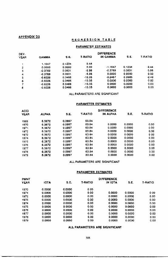
APPENDIX D3 R E G R E S S I O N T A B L E

PARAMETER ESTIMATES

DEV. DIFFERENCE YEAR GAMMA S.E. T-RATIO IN GAMMA

1 1.1647 0.1234 9.4.4 2 0,0000 0,0000 0,00 -1.1647 3 -0.3769 0,0631 -5,98 -0,3769 4 -0,3769 0,0631 -5.98 0.0000 5 -0.8226 0,0466 -13.35 -0,2457 6 -0,6226 0.0466 -13,35 0.0000 7 -0,6226 0.0466 -13,35 0.0000 8 -0.6226 0.0466 -13.35 0.0000

ACCI YEAR ALPHA

ALL PARAMETERS ARE SIGNIFICANT

PARAMETER ESTIMATES

DIFFERENCE S.E. T.RATIO IN ALPHA

1969 6.3672 0.0997 63.84 1970 6.3672 0,0997 63.84 0.0000 1971 6,3672 0,0997 63.84 0.0000 1972 6,3672 0,0997 63,84 0.0000 1973 6.3672 0.0997 63,84 0,0000 1974 6.3672 0.0997 63.84 0.00O0 1975 6,3672 0.0997 63,84 0.0000 1976 6,3672 0,0997 63,84 0,0000 1977 6.3672 0,0997 63,84 0.0000 1978 6.3672 0,0997 63.84 0,0000 1979 6.3672 0.0997 63.84 0.0000

PMNT YEAR IOTA

ALL PARAMETERS ARE SIGNIFICANT

PARAMETER ESTIMATES

DIFFERENCE S.E. T-RATIO IN IOTA

1970 0.0000 0.0000 0.00 1971 0.0000 0.0000 0.00 0.0000 1972 0.0000 0.0000 0.00 0.0000 1973 0.0000 0.0000 0,00 0.0000 1974 0.0000 0,0000 0,00 0,0000 1975 0,0000 0.0000 0.00 0,0000 1978 0,0000 0,0000 0.00 0.0000 1977 0.0000 0.0000 0,00 0.0000 1978 0.0000 0,0000 0,00 0,0000 1979 0.0000 0,0000 0,00 0,0000

ALL PARAMETERS ARE SIGNIFICANT

S.E.

0.1234 0.0631 0.0000 0.0985 0.0000 0.0000 0.0000

S.E.

0.0000 0.0000 0.0000 0.0000 0.0000 0.0000 0.0000 0.0000

0.0000 0.0000

S.E.

0.0000 0.0000 0.0000 0.0000 0.0000 0.0000 0.0000 0.0000 0.0000

T-RATIO

-9.44 -5.98 0.00

-2.49 0.00 0.00 0.00

T-RATIO

0.00 O.O0 0.00 0,00 0.00 0.00 0.00 0.00 0.00 0.00

T-RATIO

0.00 0.00 0.00 0.00 0.00 0.00 0.00 0.00 0.00

588

A P P E N D I X D 4

Residuals versus delay • • . . . . . . . . • . . . . . . . . . • . . , . . • . , . , . , , . . ~ . : ~ . • , ~ . . .

• * . . • . , . • . . . , . . . - . . . . . ' ,~ ~ , ~ : , . . . . . . f . . , ' . . , .

. . • . . . • . . . . . . . . . .

2

. . . ...,..~ . . . . . ~" , . 3 " ? ~ - . , . ' , ' , " : " , " 5 : ~ . ~ ; ' . ' " : * ~ r . . . ' . • . ~ . ~ , ' : I ~ , , ~ : . : ~ ; , . . . ~ : ; , , ~ . , , • . . . ~ , : . ~ . , . ~ . . ; , , . _ . , : , . . ~ . , . .....

0 | , . . . . . . . • • * . . . . . ' " " - : ' , " " . . . . .~ ~ 7 ' - - ~ . ~ k ~ . ' ~ , - ~ .= " . , " , . : . " , - " ' . . . . . .

I I • ' : ~ . ' " , , . . . ~ : " ' : ~ " ' ~ , ~ . . " : ~ , : : ' ; ~ . . ' . . - ¢ . ' . : . " . , : - . . ; ~ . }~" * , . , . ~ : . . ' : " ' , I

- I . ~ ' " " ' . ' ~ ' : ' . ' : ' , . : ; ' " " " . : ; ~ ' . . ~ : ' " , ' - ~ : ~ " " ' ' ' . " . , ' " I , : . * " ~ " . ~ ! ' . - ; . ' * ~ " ~ , . . ' ~ , ~ . ~ ' : . ~ , ' U ' . . " . : ~ ' . ' : - ~ . , ' ' , ' ~ : . . 5 ~ . : ~ " : I - " ; .

., " , . . : : - ' . , . . : ' r ' ) ' ' , ' ~ ' . & ' ~ ' . " : ; ' . " " " : . ' . " : : ) *I ' ~ . )~ , ; " ' : ' :~ :2~: '~S '~ ' :U~" ' : . . , ," ..: ' ~: '¢%~i ' .~ '~ '~ ' '~ ~"' • . . . . . ~ . . . . , f . . . . . , ~ . . . . ~ • , . , ~ . . . , , . . . . . . . , . : , , : . . . , : . ~ . . , ; : : . . , ~ . ~ . ~ . . . ~ _ . , . , ~ . - . , . . . . . : ~ : g , : . . , ~ ,

' . ' • ~ , . . - . : . " ,.: - • " . : . ' 7 . . ~ . . . . " = " " . ' , ~ , i ~ ~ . : . , ~:,, : , : '~ ~ : ~ . '.,....' ~ . . - ' - o . ~ : , : , ~ . ~ " J " ; ) ? ' ' ~ . - 2 • . y " . , ' : . . . . ~ . : : . ~ ' ~ . - - . ' . . . - . . , . " " " . . . . . . . " . . . , . ~ : : . . . . ~ , , . ~ ' : , . ~ . : . . % . : ; " . . ' . . . ! , ~ ' . . " ' ! : . . . . . .

• . . . . . . , : . ; . : ,. • • . . . . . ~ . • , . . ; , . : . .~ . . .~ :~ . , - ~ , v ~ , . ~ . . . . . . , , • , . . .

• 3 " I ~ ' " ' I " " "" "1: " I " " I ' " ' " " "" "i ~" " I ' " " "1 '

0 I 2 3 ,~ 5 6 7 ! 9

F i g u r e D 4 . 1

Residuals versus accident years • . . , . :,;,~,:..~.%",:.,~; :: . . . . . . . " ~ , / . : : : A ~ : : : " . U . ~ : ~ : : . I ¢ , I ~ : . . ' . " .:: . • .

' i i i ~ ! ~ ' : ~ , + ~ i : : ~ : ; ~ ! ~ : ?: :~: : . . . . ~ , , : , , - : ~ - ~ ~:;..~!~,~.:~:i~ : : I • ' ~ : S ' ~ , ' ~ ~ . . :. ~ ~ ; ~ , : C ¢ '~,~ ' . . . . . . . . . : . . . . :~ " ~' ' • . . . . . ~; • . : ':~ "

z I!~i:,!::~ ~i~;~::, i : ~':.~'?~ ~ ~ ;;"~...~,~,.'; . . - . - " " " • . " : : . • . ~ . . . . . . . ' : • ~," ' ; " '~:" " ' ~ ~') , :~". . : . " . '~ : , ~ ' . : , " "" " . " • ' : • " . ' ~ ." "~ ; " " : ~ " ~ I ' " , ". , ' " • "" "

.".'~.~'~:~::~.:~ :~ ' : ' " : :~ -~ . ' : .:.' .V ' : ,~ , , " ' " ° .~ : , " . : ' ~ ' ' f ' : ' : ' . • . " -

' i?i~i':: ~'`:~!~:!!~!' , , • . ~ ; ~: 7 :~! ' : , = ~ . . : : : t ' - " . . 5 : : ' . . . ' : ' . . :

• . o • | | • . . : . . ~ . . . . . . .

- I

- 2

. J

1 9 6 6

" " I . . . . . " I .: . ' . . . ~ ' . . : . . . . . : • '

• : i / ~ ' ' : ' t ? ~ : . ' ~ . ) . .

• .~ . . , . . :

| " ~ I

1 9 6 | 1 9 7 0 1 9 7 2

I

, . . , . • ~ i ~ : . . , : ' ~ . ~ . i . , • " ' :

• ~ . . . . . : . . : . . " ,:~', .,...:. ~.: , ' . ' : ' . ; . . . . . : . . . - . . • .

. . . . "1 " : ! " "!

1 9 7 4 L 9 7 6 19711 1 9 1 0 1911

F i g u r e D 4 . 2

5 8 9

APPENDIX D4

Residuals versus payment years

I ~ 1961 1970 197l 1974 1976 197I 1910 1912

Figure D4.3

590

APPENDIX D5

DEV. YEAR

ACCI YEAR

1969 1970 1971 1972 1973 1974 1975 1976 1977 1978 1979

PMNT YEAR

1970 1971 1972 1973 1974 1975 1976 1977 1978 1979

GAMMA

1.1777 0.0000

-0.3478 -0.3478 -0.6749 -0.6749 .0.6749 -0,6749

ALPHA

6.4594 6.4594 6.4594 6.4594 6.4594 6.4594 6.4694 6,4594 6,4594 6.4594 6.4594

IOTA

0.0000 0.0000 0.0000

0.0000 -0.4792 0.3723 0.0000 0.0000

0.0000 0.0000

R E G R E S S I O N T A B L E

PARAMETER ESTIMATES

DIFFERENCE S.E. T-RATIO IN GAMMA S.E.

0.0993 11.86 0.0000 0.00 -1.1777 0.0993 0.0519 -6.70 -0.3478 0.0519 0.0519 -6.70 0,0000 0.0000 0.0390 -17,32 -0,3270 0,0803 0.0390 -17,32 0.0000 0,0000 0,0390 -17,32 0.0000 0,0000 0,0390 -17.32 0.0000 0,0000

ALL PARAMETERS ARE ~GNIFICANT

PARAMETER ESTIMATES

DIFFERENCE S.E. T-RATIO IN ALPHA S.E.

0.0927 69.68 0.0927 69.68 0.0000 0.0000 0.0927 69.66 0.0000 0.0000 0.0927 69.68 0.0000 0.0000 0.0927 69.68 0.0000 0.0000 0.0927 69.68 0.0000 0.0000 0.0927 69.68 0.0000 0.0000 0.0927 69.68 0.0000 0.0000 0.0927 69.66 0.0000 0.0000 0.0927 69.68 0.0000 0.0000 0.0927 69.68 0.0000 0.0000

ALL PARAMETERS ARE SIGNIFICANT

S.E.

0.0000 0.0000 0.0000 0.0000 0.1306 0.1182 0.0000 0.0000 0.0000 0.0000

PARAMETER ESTIMATES

DIFFERENCE T-RATIO IN IOTA S.E.

0.00 0.00 0.0000 0.0000 0.00 0.0000 0.0000 0.00 0.0000 0.0000 -3.67 -0.4792 0,1306 3.15 0.8515 0.2330 0.00 -0.3723 0.1182 0.00 0.0000 0.0000 0.00 0.0000 0.0000

0.00 0.0000 0.0000

ALL PARAMETERS ARE SIGNIFICANT

T-RATIO

- 11 .86

-6.70 0.00 -4.07 0.00 0.00 0.00

T-RATIO

0.00 0.00 0.00 0.00 0.00 0.00 0.00 0.00 0.00 0.00

T-RATIO

0.00 0.00 0.00

-3.67 3.65 -3.15 0.00 0 O0 0.00

591

APPENDIX D6

( R E G R E S S I O N O U T P U T C O N T I N U E D )

S = 0 . 2 6 5 4 S . S Q U A R E D = 0 . 0 7 0 4 S - S Q U A R E D ( S C I ) = 0 . 5 4 6 9

S(B) = 0 . 2 6 5 4 S ( B ) . S Q U A R E D = 0 , 0 7 0 4 D E L T A = 0 . 0 0 0 0

R - S Q U A R E D = 93 .5 P E R C E N T N = 62 P = 6 .0

SSPE = 7,:360 W S S P E = 7 .360 A IC = 17.13 A IC(SCI ) = 43.81

592

APPENDIX D7

Residuals versus delay

0 I 2 3 4 ~ 6 7 I 9

Figure D7.1

Residuals versus accident years " :~ .~ : . : . . : .~ :~¢ .~ . `~ : .~ '~ .~ .~2 :~ :~ i :~ : : :~ : ; .~ : / : ;~ ; : . . . ; . . : . : ; . . i . .~ - ; :~ : .~ ;~ :~ . . .~ . .~ :~ :%.~ .~ ~ ~'::::~.?~~:~.,~:Y~.~'.!::i!;:~::~:~!~,.', " ~ ~ ; : , : :

I

z L ~ . , ~ . ~ . ' ~ , ~ : ~ ' : ~ f f ~ ' ~ " ~ . ~ : , ~ :~ " ; o. " .". '. :~.~ ~ "L.,- ~'~ ~ : ~ : : , ~ , ~ : : ~ : ! ~ : ~ . ~ , , : ~ , ~ : ~ ; : .., ~r.!....:.'~". • ~ ,.-. .., I

o . . . . . . . . . . . . . . . -:-::%~.:~.!;~..~ii~;~i~;~!i!:~ ; ~ i ..~::i:. . . . ,. ,.~.~i~.~,~ .~ . . . . !i, S . ~ . ~ 2 ~ , ~ : , w . . , , . : ~ : - ~ , , • ~ ; ~ ~ : ~ :~;"~'_~."i~~.,.',.~.~:~', . . ? , ; . i~ . : . . . . . . . :;:.':;,.? ~:.:~. :, . . . , ; , - . ~ : , . ~ : ~--.~:,~-~..,..~ ~-~... . , . • ,s:i..,< , . . , . . k - , ~ : ~ , ; . : ~ . ~ , ~ . ° . ~ , ~ , . , . t ~ , ~ . ~ . ~ , ~ . ~ , ~ ¢. ..e,!.,..~ ~ , z . , r . . . . . :

F • ~',:: ~::,~ :~.?,.'~;:. ',..:z~j'~.'::~!?~" :.~ ; , ~ ' ~ ~ ; . : ~ . . : ~ ; . i ~ . ~ ? ' : . ~ ~ i . ~ , ~ : , 3 ~ ~ ? ~ . ~ . , ' ~ , ~ . t ~ , r : ; . .. , ; r • , : : ~ : " I I ~ , " . . . . . . . ~ : : r ~ : : t ~ i ~ : ~ - . . : ~ 3 ' ] ~ ; T m z ' . " . ': ,~:.'.f ~ . : ~ : ~ : ~ . . ' : T ~ : . . ~ ' : ~ : ~ ' ~ ) ~ , ~ - ~ . ~ % ? ~ r . : ' ° ~ " ~ : ~ ; : ' : . : : - ~ ' , . ~ ; : ~ ' ; g l

I ~ . . :~ ~...; .'~'.~': :.~:~w ~ .,: ,:'~::. ° . ' : , : ~ . . . .~.'.~:...% ~ :,~:,~ / ~ : ~ ! z ~ . . ' . ~ : ~ c , ~ . L ~ 7 ~ : ~ : ~ : ~ . : . ~ :÷~'.:...::~7~:~!~'~:-;. :1

"~ I . : :~ ~-~ ; - ; :~,.:~.-~. • : . . . . . . . . " "... ,-,.o~ : . . . . . . . . . . ~o: ~;~'~-~ ,:~: ,~ -~ ~ ' - ~ ' ~ 3 ~ : E . - ' i ! ~ i ~ ! ; : ~ ' ~ 7 ~ ~ . ~ : - ~ ; ' ~ ' ~ . ~ . ~ :~ . u - . . " ...: . . . . . . . . . . . ~ . . - ~,.. :" , : .... • "' ,:~ :".z~.-'¢:~t~':i,.~;:- :~ ,~ ,~ .~ . : .~z~L:~ , . % ~ t ' ~ , ~ ; ~ ' ~ . ~ - , ~ : ' . ~ : ; . : . ~ . ~ ¢ : " ~ 4

.~ I : " > " " : , ~ . . . . , .... , ' . . . . . ' i " ~ ' " ' ~ ' : ~ " : - ' ~ " : " : " " ~ " ~ : i : ' . ~ " . . . . . . . . . . , . . . . . . I 1966 l ~ l 1970 1972 1974 1976 1971 1910 1912

F i g u r e 0 7 . 2

5 9 3

APPENDIX D7

Residuals versus payment years ~ ' .~ : : , . • ~ ° ~ ' ~ ` : ~ ! ~ : ` ~ ` ~ ` ~ ` ~ : ` ~ : ~ ` ~ ; : ~ ` ~ : ~ : ~ ! ~ : ~ L ~ ` ~ L ~:~:...%X:i:~F~.~i~,.:~..9:.;~!:~:,i!~...~i).~i.'~,':; ..,".... " . . . . . . . . • ' " ~ ~ . ~ " ~ - :~ ~ " : ~ ' ~ : . ~ : " ~. <i.~.~c.': ;::.~ :~.~:.~! . . . . . , . . . . " . ' , , • " , " :i~::"a~~"~i-~:'.~ '~:;.' i'~>~'~'~~6:~z~ .~.~.' ~:t~.~; ..v.:. ~ . ~ ":'~',:~::,~;~!~::~.LS;=~'z.".~:L'f~,~:~5.~.~;~.~:::~.~:.:-,.:.~. `.

• " - ~ " : , . ~ : " " " .~ . . " '~ ' : . . '~ , i ; ' . : ' . , . : , i ! " ~ : . ~ ; ~U" : ~ ! ~ ' . ' ~ ; ~ . ~ , ~ ' ~ : ~ ' ' : ~ : ' ~ ' ~ L % ~ ' ~ : , ~ Z ~ I I ' ~ . ~ " ~ " ~ ' ~ ; : ~ < ' : ~ " ~ , ~ P : ' ~ ' ' ; ' : ' ~ ' ~ ' : ' ~ ' ' ~

0 ] ~ = ' " , ( . : : . ~ . : ; i ~ , i . : ; : ! . : : z ' ~ . : ~ : . ~ . ~ : i ~ ! t ~ i . ~ . ~ . ~ ' . ~ , ; : . r Y : :,~,,~;~.ct:>'~.~i~'~:%.. ;~'r:'.,~=~!~:.~i:~;!~,.~;F;i~.'~.~?.~t~.~t:;:~¢:.., ' : .::~ . .

19~,a ~,.~;: : " ~ '¢>: i~.'~ ' ~ : ' ! : . ' .: :~ ~. '~~:~.;~-.. ' . .~..:, ' . .~..-.~.~....~..:~;~ . . , . . | , L"; ~ ~ , :i~"~:~::¢'~e ~.~ ~ . . . . . . . : ~

19~11 19710 19'/'~ 197/4 19"76 19711 19110 1912

F i g u r e D 7 . 3

Residuals versus fitted values

4 $ 6 7 | 9

F,3oc~ D7. 4

5 9 4

APPENDIX D7

Normal scores versus residuals :: " . : , • ..,: *"vii:: :~,:~:,,~".~:~,~,,:~,:.~i.~:~~':?:~";i.77~.~:~i~'~ ; : ; .~:~ , : ;~" ."£~~i~ .~4"~~ '~": . '~~! '~ t ' i :? ' :~ " : 7. ~" ~ " ' ~ ~

~:~,i ~[ :~ .~;~: ,~ .~;~.~:.;.~, .~i~ ~;;.~.~:.!~:.~i~!.~.:~': ~.$ ~ ~::..'.~:: :..'.~ .' i:!~ ~ l,.;~'-~.'."~[-. ~'~'.~ '~i;~.~,~..~ k ~ ~.~ ~ .p~ i~ - ~ ~'.~', :: ~ ':~ :" ~i~"o:.~ !; :.~.:: [ ~,. ~ .i:,~:~..."~:~..:?~:~P~.~!~:.~: ~ ' ~ : ~ ' . ~.~]~{;~.~.~,~v~, ~ i ~ , ~ ~ ] ' ~'~:~',i~.]:~ ~ . ~ ~ : ~ . . . ~ . ~ ;o .~.;£,::. ~/: • i~:,;-..".'~: ~ I -:~...'.: ~! ~< ~<:, .~ ~.~: ~ ~: ~ :~ ~ ~!~:.~:,,~ ] ~:. ~ ~ ~ ~:i,~ ~ ~ . ;~.<,~.~.~..,:~;~.~.~ ~ : ~ ~.~.,~.~.~:::~.',~ . /

. . . . ~ . , , , ~ :< ; ~ . ~

.Z -1 0 I

:.~..~.~.k~ ~ ~. ~ : ~ ,.

Figure D7.5

5 9 5

F O R E C A S T I N G O U T P U T

ASSUMED FUTURE INFLATION = 0.0000 STANDARD ERROR = 0.0000

EXPECTED PAYMENTS/OBSERVED PAYMENTS + . . . . . . . . .4- (PAYMENTS IN $1 S)

FORECAST MEAN PAYMENTS/STANDARD ERRORS

EXP: 346295 1123112 1123112 793172 561671 177321 130329 66469 33951 OBS: 193013 1584331 1151882 778980 475203 143352 128612 70845 25077

EXP: 425750 1380806 1380806 975161 428440 314654 160233 81720 41741 OBS: 376473 1541950 1719509 1032570 289305 382508 270087 108354 23133

EXP: 447601 1451671 1451671 636733 650595 330803 168456 85914 43883 OBS: 568891 1579158 1277822 734670 680369 217221 147800 57099 64829

+ ......... 4 EXP: 445614 1445229 898519 915576 647708 329335 167709 85533 I 43689

m

OBS: 428753 970640 955898 1095771 510072 491853 242995 299845 I 12280 + ......... +

EXP: 535664 1080091 1559962 1100596 778597 395887 201599 102817 52517 3BS: 458252 989072 1417606 953222 881133 278778 197156 27673 14762

+ ......... + i EXP: 275565 1290006 1290006 910134 643858 327378 I 166712 85024 43429 ~BS: 355229 948807 f292900 748003 547288 274367 I 43841 22884 12207

+ . . . . . . . . +

~XP: 305191 989197 989197 697906 493721 251038 127837 65198 33302 )BS; 282419 688332 1158793 903450 629983 65999 33618 17546 9361

÷ ......... + I

~XP: 323039 1047045 1047045 738719 J 522593 265719 135313 69011 35249 )BS: 267600 1044790 1216437 527644 I 140549 69858 35584 18574 9908

+ ......... +

!XP: 370037 1199377 1199377 846194 598624 304378 155000 79051 40378 )BS: 560307 940002 1185899 221766 160997 80022 40761 21276 11350

+ ......... + !XP: 418225 1355566 1355566 956389 676580 344016 175185 89345 45636 )BS: 360171 1011773 360708 250646 181963 90443 46069 24047 12827

0

0

0

0

O

0

43689 1228O

155334 32822

295165 53323

477376 79132

1027886 167258

2023625 300456

3642717 502218

4 .......... + :XP: 442022 1432697 1432697 1010807 715077 363590 185152 94429 48233 5282681 )BS; 445545 381231 381231 264907 192317 95589 48690 25415 13557 674135

. . . . . . . . . . . . . . . . . . . . . . . . . . . . . . . . . . . . . . . . + . . . . . . . . . . . . . . . . . . . . . . . . . . . . . . . . . . . . . . . . . . . . . . . . . . . . . . . . . . . . . . . . . . . . . . . . . . . . . . . . . . . . . . . . . . . . . . . . . . . . . . . . . . . . . . 4 . . . . . . . . . . . . . . . . . . . . . . . . . . . . . . . . . . . . . . . . . . . . . . . . . . . . . . .

PAYMENT YRS: ! 4721306 3518808 2235705 1316405 653075 314876 140065 48233 12948473 30 ERRORS: i 623018 504462 345451 223516 111688 57649 29752 13557 103080~

APPENDIX D9

ACC. YEAR EXPECTED OBSERVED

(PAYMENTS IN $1'S)

69 4355433 4551295 70 5189312 5743889 71 5267328 5327859 72 4849689 4695982 73 5652397 5175219 74 4736946 4166594 75 3475212 3662977 76 3155847 3056471 77 2768792 2686208 78 1773792 1371944 79 442022 445545

TABLE OF OBSERVED AND EXPECTED BY YEAR

DIFFERENCE

$95862 554577 60531

-153707 -477178 -57O352 187765 -99376 -82584

-401848 3523

PMNT %ERROR YEAR EXPECTED OBSERVED DIFFERENCE

(PAYMENTS IN $1's)

4 69 346295 193013 -153282 9 70 1548863 1960804 411941 1 71 2951519 3262723 311204

-3 72 4071263 4506400 435137 -9 73 4969396 4214487 -754909

-13 74 3496670 3467526 -29144 5 75 5166314 4936092 -230222

-3 76 4908050 4270279 -637771 -3 77 4708472 5166110 457638

-29 78 4697662 4569353 -128309 0 79 4802265 4337196 -465069

%ERROR

-79 21 9 9

-17 0

-4 -14

8 -2

-10

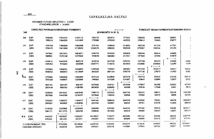
4DI) F O R E C A S T I N G O U T P U T

ASSUMED FUTURE tNFLA]ION = 00000 STANDARD ERROR = 0.0000

EXPECTED PAYMENTS/OBSERVED PAYMENTS EAR

+ . . . . . . . . 4- (PAYMENTS IN $1 S)

FORECAST MEAN PAYMENTS/STANDARD ERROrri

169 EXP: 346295 1123112 1123112 OBS: 193013 1584331 1151882

J70 EXP: 425750 1380806 1380806 OB S: 376473 15,41950 1719509

171 EXP: 447601 1451671 1461671 OBS: 568891 1579158 1277822

J72 EXP: 445614 1445229 898519 OBS: 428753 970640 955898

}73 EXP: 535664 1080091 1559962 OBS: 458252 989072 1417606

~74 EXP: 275565 1290006 1290006 OBS: 355229 948807 12929QQ

175 EXP: 305191 989197 989197 OBS: 282419 688332 1158793

J76 EXP: 323039 1047045 1047045 OBS: 267600 1044790 1216437

=77 EXP: 370037 1199377 1199377 OBS: 560307 940002 1185699

~78

793172 561671 177321 130329 66469 33951 778980 475203 143352 128612 70845 2507?

975161 428440 314654 160233 81720 41741 1032570 289305 382508 270087 108354 23133

636733 650595 330803 168456 85914 43883 734670 680369 217221 147800 57099 64829

+ . . . . . . . . +

915576 647708 329335 167709 85533 I 43689 4368' 1095771 510072 491853 242996 299845 I 12280 1228,

+ ......... + i 1100596 778597 395887 201599 ] 102817 52517 15533 953222 881133 278778 197156 I 27673 14762 3282

÷ ......... + I 910134 643858 327378 ~ 166712 85024 43429 29516' 748003 547288 274367 I 43841 22884 12207 5332

÷ ......... +

697906 493721 251038 127837 65198 33302 477371 903450 629983 65999 33618 17548 9361 7913:

+ ......... + !

738719 ~ 522593 265719 135313 69011 35249 1027861 527644 I 140549 69858 3558~ 18574 9908 16725~

+ ......... +

I 846194 598624 304378 155000 79051 40378 202362! 221766 160997 80022 40761 21276 11350 300451

i + ......... ÷ EXP: 418225 1355566 1355566 956389 676580 344016 175185 89345 45636 364271, OBS: 360171 lO 11773 360708 250646 181963 90443 46069 24047 12827 5022 I

+ ......... ~79 EXP: 442022 i 1432697 1432697 1010807 715077 363590 185152' 944229 48233 5282r~L

OBS: 445545 | 381231 381231 264907 192317 95589 48690 25415 13557 67413'

) T.FOR PAYMENT YRS: I I 4721306 3518808 2235705 1316405 653075 314876 140065 482233 1294 84 /

fANOARD ERRORS: I 623018 504462 345451 223516 111688 57849 29752 13557 103()HH~

APPENDIX D1O

VAU DATION

OEV. YEAR GAMMA

1 1.2466 2 0.0000 3 -0.4024 4 -0.4024 5 -0,5544 6 -0.6544 7 -0.6544 8 -0.5544

ACCI YEAR ALPHA

1969 6.4278 1970 6.4278 1971 6.4278 1972 6.4278 1973 6.4278 1974 6,4278 1975 6.4278 1976 6.4276 1977 6.4276 1978 6,4278 1979 6,4278

PMNT YEAR IOTA

1970 0.0000 1971 0.0000 1972 0,0000 1973 0.0000 1974 -0.4798 1975 0.3067 1976 0.0000 1977 0.0000 1978 0.0000 1979 0.0000

R E G R E S S I O N T A B L E

PARAMETER ESTIMATES

DIFFERENCE S.E. T-RATIO IN GAMMA S.E. T-RATIO

0.1076 11.58 0.0000 0.00 -1.2468 0.1076 -11,58 0.0639 -6.29 -0.4024 0.0639 -6.29 0.0639 -6.29 0.0000 0,0000 0.00 0.0753 -7,37 -0,1520 0,1213 -1,25 0,0753 -7.37 0.0000 0.0000 0,00 0,0753 -7.37 0.0000 0.0000 0.00 0,0753 -7.37 0,0000 0,0000 0.00

ALL PARAMETERS ARE SIGNIFICANT

PARAMETER ESTIMATES

DIFFERENCE S.E. T-RATIO IN ALPHA S.E. T-RATIO

0.0922 69.72 0.0922 69.72 0.0000 0,0000 0.00 0.0922 69.72 0.0000 0.0000 0.00 0,0922 69.72 0.0000 0.0000 0 00 0,0922 69.72 0.0000 0,0000 0.00 0,0922 69.72 0.0000 0.0000 0,00 0,0922 69.72 0,0000 0.0000 0,00' 0,0922 69.72 0,0000 0,0000 0.00 0.0922 69,72 0,0000 0,0000 0.00 0.0922 69.72 0,0000 0.0000 0,00 0,0922 69.72 0.0000 0,0000 0.00

ALL PARAMETERS ARE SIGNIFICANT

PARAMETER ESTIMATES

DIFFERENCE S.E. T-RATIO IN IOTA S.E. T-RATIO

0.0000 0,00 0.0000 0.00 0.0000 0.0000 0,00 0.0000 0.00 0.0000 0.0000 0.00 0.0000 0.00 0.0000 0.0000 0.00 O, 1206 -3,97 -0,4796 O. 1206 -3.97 0.1203 2.57 0,7686 0.2196 3.59 0,0000 0.00 -0.3087 0.1203 -2.57 0.0000 0.00 0.0000 0.0000 0.00 0.0000 0,00 0.0000 0.0000 0.00

0.0000 ALL 0 O0 0.0000 0.0000 0.00 PA~AM~TEIZS ARE 5~61,1ilCieANT

599

A P P E N D I X 0 1 1

All residuals versus delay

-I 0 1 2 ] 4 S iS 7 I

Figure 011.1

All residuals versus accident years

0,5

..0.5

-I

1 ~ t ~u.w Isr'~o 1 ~ 1974 1976 19'/11 1910 |952

F!gure 011.2

600

A P P E N D I X D I 1

All residuals versus payment years I.S

-0,3

.1 is~,6 19611 lsrto 1972t t974 19'76 19711 19|0 t~ ,

F i g u r e D1 1 . 3

Z.J All residuals versus predicted values

0.5

..o.s

.! 4 4.5 $ 5.5 fi ~$ 7 7.5 | I.s

F i g u r e D 1 1 . 4

A P P E N D I X O 1 2

Validated residuals versus delay Vahda~cd r~ si cb.~a I =!:~'~ d.t c t ~cn cntor

I . ~ , . . , . , " . . . . : : . , . ~ . " : ~ • • ~ . • . . . . - . , , : 7 . : " "~ - " -

~: : ~ ..... . , ~ : ~ : i ~ , ~ , : , , . ~ o . . ~ , ~ , ~ . ~

o, i: ii : i . !ili i ;: i o , [ , : - : ' , : : , ' • :~-., • : ' " , : . . . . ' , . . . . ' • . '~":. : . ' : ' " : ' ~ ~ ' 2 ~ " . , . ~ . : ' " . ~ ' . : " " : ' " ' ~ : . " . . . " ' . • • "

I • " "? ' ; : ' " " ~ " = " " " : " " ' ; ::~~:~ ' : " : ~; ' : : " " ' ~ ' : " ' • . i . . . . : ' • ,~:~::,~.~,,'~:~,'. ~.~:.:.~-~: . ~ , : i~ ':.: ' . . " . : . . " " " . "

::.~.~...:~°..~ ....~ . . : . . . j ~ ; . . / . . . " .. . , , , . . . . . ~ . ,:.. :~ !~ ' , . ; :~ :~, , : . . :~ .~. . ,~,~ '~ . . ' . ' . . . . . , • . ~ . ~ . ~ ..:..:." ,

• ~ ' ~ : . . . . . ' " . ~ "~" ' :~ ' : : . . . . . ' ' " " " :'~ ~'~.~ ~, ' ,~: ' ;p~.~::~:.~"~:~:~ '~ ~ : . . ; . - ' ~ • " ~ ,~ . : ~L , ' . - " . ~ ~. . . .~ . . . . . . . : , • . , . ,< . . . . . ~.. • . , : ~ .... ,~: . .~. . ,~.~. : .~. . : . ' . . . , : ' r . . . ~ . " . . . . . . , : .. ' ~ o • . . • . . '; , . ' : . . . . . , . ' > ~ ." . ' ~ . . . . , . . , . . . . . . . . • . . . , . . ; "..+.~. % ~ ~"~,~++~ ' ' ~ ' : : " ~ " ' : ~ ' . ' : " '~ " ~ . , . . :: : , ' . . . ~ . < ' ' ~ .. •

.1 ' , ~ , " , , '~:~"~:"~':'i:"~'::':~::~ i ~ " : J ? ~ " o 1 ~ 3 ~ 5 66 7 |

F i g u r e D 1 2 . 1

Validated residuals versus accident years . ; ~ : ~ ! , ~ : ~ : ÷, . . . ~ ~ . ~ : % ~ ! ~ ! ~ . , ~ ~ . . . , . : ~ : . . • ~ . . " . . . . . . . : , : .~ . . :~ , : . : ;~ .~; , .~ , i . ! . ~ . ~ : . ~ 7 . ~ . ~ . ~ , . . ~ . ! ' . . : : . .~ ~.:~'.:~,~ ~ , . . .

~ , . z ~ . : . : ~ . ~ . ~ o . ~ . f ~ . ~ : : , . ~ . . . . . ~ . . ~ . ~ . . . . : ; . : , : ~ . : . . . ... . , .. • . . : . : . < . : . ~ , ~ .~ , : . ~ ~ : . . . . : ~ . .. . . , , ~ . ~ : : . : ~ : , - . . . . . . ~ ~ . ~ ! ... . . . ~ ' ~ : . ' : : ~ . ~ . ~ , ~ , ~ ! ~ . ~ . $ : : ~ ' o : ; ~ ~ . ~ ; ~ . . ~ . . ~, . . . . . . . : . . . ~ . ~ : . ~ . : , . ; . . ~ ~ : ~ : ~ , = ~ . , % . . - , ~ - . . : . . , ~ ~:::~,~.- , • ,

~ . ~ .~:.:,~!~,~:,~.-• ~ : • :.... ~ . .~,~, ,~ ~,~:,~:~.!~.~:.':~.!~.,!.~.

~:.~.,,~::.~,.....~':...-.:~,::t~'.:;.~":::~ . . . . . . . " " • . " " : " ..'.~-.: ...... !,-:'!~: ." ' : . :",.: ' .-~-:~ , : ; ~ . " .~:~"

: : Y " : , ~ " : ' ~ ; i " : ~ : : " : ~ " ~ " ~ : ~ ? ' . : " : , ' . . . ' • ' . , ~ C " : . ° : ; . : j i ~ , . : ~ , :~ .~-~ ' ;~ . r : . '~%~,~ ' ,~ ' : : " i - : : ~1 : : : . ~ : ~ ~ . ' . " ~ " . " ~ ' ; ' ~ : ' ~ " ~ ' ~ : . : ~ ' . ~ " • ' ~-.". " - . " . ~ ' ~ ~~':~','-",~ ~ . . : ' , t " ~ : ~ ~' : " ! : ~ : . . . . . . ~ ' . " ~

• .. .'-.::.:L ~, ~. ' : ~ ~ : ~ . ~ . ' ~ . "..~ '.:.~ ,.... . . . . . ~ :r.... : . ~ . . . :~ '~ . ~ . : ~ : ~ , t ~ q i ~ i ~ " . ; ; " . ~ ' ~ :~:~.~°'~ • : :~:~:~, , ' : - , ~ : : , :~ ' .~ : : ~ : ~ i ? ~ : ' , i " ~ . . . ~ L ~ : ~ i ' : " ~ i ' , , , .~C.~." . . .~ . , * . :~ :~ '~ ~ . ~ . ~ : < ~ . ~ . ~ : . ~ ~ . ~ . ~ . ~ . ~ .: ~ : ~ . " . . " ~ . . ~ t ~ ' . . . . : : : . ~ . . . ~ ' . ~ . ~ : : ~ ~ : ? : : . . , ~ ~ . ' ~ ' ~ : . , ~ ' . .. • . , . . . . . ~ = , . . : . ~ , . , . . . . . . ~ ; . ~ . ~ - . ¢ ~ . - . . . :~ : , . , ! • .. ~,.~ ...::: ..-~ ~ : . . . . - i~.~.. . : .~.~,/ :~!. : . , , : . . .~,!~..~:: i . ,?..~.. . . ,%.%:.. i~:. . . : . / . " . . . , ~ , . ~ : . ~ . . : . ~ , ~ , ' ~ ~ ~ ~o~*~ ' .~o~C~,~, '.~. ., : . . " . . . . .

. . ..,.~ • . . . . . . . . . = = . : ~ , : ~ . ~ / ~ : ~ . ~ , . ~ . ~ . ' ~ = ~ . : , , ~ ~ .~.~, . . . . . ~-: . , . . . . . ' . . .

. . , ~ . . , ' ~ ;~ : . : . ~ , . = ~ , . . ~ ; ~ . . , ' , ~ " ~ . . , , : : ~ , , : ~ j . " . . . . . . : ~ .o . ' . . . . . - : . . ~ . ! . : ! : , . ~ :~ .~ .~ .~ .~ ,~ ,~ .T . . . . ~ .~ :~ . ;~ . . . , ~ : : : . ~ ;~ : .~ , : :~ . ~ , : . . . . . ~' : .'~'~ , : ~ .~ i ~.~.~,~'~..~ .~~...~-:~.~,~ ~:. ~ . ~ f.~!~,~ ~ % , . . . . : ' , : : ' :.., '..~ " •

• i ̀ :~: ; : , : : : : ; :~ i~! i : :~: : ; : : ! i~ i~:~;~, : ;~; ~ii',~ ~: !" - I ~ . . . . . . . i " ' ' " " l ' : ' " " " . & " ' " 1 , . ~ " : : " ' ~ ' . ; ~ ' : h " - ' . ' . . . . . I ' " " ~

19,66 1~1 1970 1972 1974 19"/6 L971 1910 191;

0,5

. 0 . ~

F,~.e~ DIZ.Z

6 0 2

A P P E N D I X D 1 2

Validated residuals versus payment years

0.$

.03

-I I Sl"/6.$ 19"/'/ 19'77.$ 19"71 19"/1.5 l~r'/9 | 91~;~,:

F i g u r e 0 1 2 . 3

Normal scores versus residuals

-I .0.$ 0 0.I$ I I.~

F t g u r l 0 1 2 . 4

F O R E C A S T I N G O U T P U T . IDATION MODEL

ASSUMED FUTURE INFLATION = 0.0000 STANDARD ERROR = 0.0000

~R EXPECTED PAYMENTS/OBSERVED PAYMENTS

(PAYMENTS IN $1 2) FORECAST MEAN PAYMENTS/STANDARD ERROR:

EXP: 333078 1157384 1157384 ORS: 193013 1584331 1151882

774069 519825 184730 144344 83624 48721 778980 475203 143352 128612 70845 25077

) EXP: 409501 1422941 1422941 ORS: 376473 15419,50 1719509

951676 395746 308064 177464 102811 59900 1032570 289305 382508 270087 108354 23133

EXP: 430518 1495969 1495969 OBS: 568891 157915,8 1277822

EXP: 428607 1489330 925009 ORS: 428753 970640 955898

EXP: 515220 1111935 1510497 OBS: 582529 989072 1417606

EXP: 264794 1249101 1249101 ORS: 355229 948807 1292900

EXP: 275840 957831 957831 ORS: 282419 688332 1158793

EXP: 291071 1013844 1013844 OBS: 267600 1044790 1216437

EXP: 334450 1161346 1161346 ORS: 560307 940002 1185899

+ ......... -F I E XP: 378003 1312583 [ 1312583 ORS: 360171 1011773 I 318349

+ ......... +

1387267 1387267 EXP:

FOR PAYMENT YRS: ~DARD ERRORS:

399511

620480 565416 323874 186571 108087 62974 734670 680369 217221 147800 57099 64829

+ ......... + I 839313 562907 322437 185743 107607 I 62695

1095771 510072 491853 242995 299845 I 20985 + . . . . . . . . + i

1008922 676660 387595 223278 I 129353 75364 953222 881133 278778 197156 I 36802 25226

+ ......... ÷

834325 559561 320521 184639 106968 62322 748003 547288 274367 46231 30433 20860

+ . . . . . . . . +

639774 429081 245780 141584 82025 47790 903450 629983 58502 35451 23336 15996

+ ......... +

677187 454173 260153 149864 86821 50584 527644 113657 61923 '37524 24701 16931

+ ......... + I 775710 520250 298003 171668 99453 57944

184214 130192 70932 42983 28295 19395

876727 588000 336810 194023 112404 65489 208204 147147 80169 48581 31980 21920

926612 621456 355974 205063 118800 69216

OBS: 445545 336463 336463 320050 155519 84731 51345 33799 23168 .................................. ~ ................... + . . . . . . . . . . . . . . . . . . . . . . . . . . . . . . . . . . . . . . . . . . . . . . . . . . . . . . . . . . . . . . . . . . . . . . . . . . . . . . . . . . . . . . . . . . . . . . . . + .........................................

4552200 3368314 2106825 1264545 700034 375411 184289 69216 578766 453677 299060 193348 117101 77112 47562 23168

0 0

0 0

0 O

62695 20985

204717 52836

353929 72717

517179 85810

1001596 147670

1923027 262653

3486O36 452821

5071655 625691

12620833 10720~9

A IDlY

TABLE OF OBSERVED AND EXPECTED BY YEAR

ACC. YEAR

69 70 71 72 73 74 75 76 77 78 79

PMNT EXPECTED OBSERVED DIFFERENCE %ER YEAR EXPECTED OBSERVED DIFFERENCE

(PAYMENTS IN l l "S ) (PAYMENTS IN $1's) . . . . . . . . . . . . . . . . . . . . . . . . . . . . . . . . . . . . . . . . . . . . . . . . . . . . . . . . . . . . . . . . . . . . . . . . . . . . . . . . . . . . . . . . . . . . . . . . . . . . . . . . . . . . . . . . . . . . . . . . . . . . . . . . . . . . . . . . . . . . . . . . .

4403160 4551295 148135 3 69 333078 193013 -140065 7251043 5743889 492846 8 70 1566886 1960804 393918 5289859 5327859 38000 0 71 3010843 3262723 251880 4753347 4695982 -57365 -1 72 4121587 4506400 384813 5434107 5175219 -258888 -5 73 4972020 4214487 -757533 4477402 4166594 -310808 -7 74 3502693 3467526 -35167 3260356 3662977 402621 10 75 4892575 4936092 43517 2996847 3056471 59624 1 76 4655693 4270279 -385414 2657142 2686208 29066 1 77 4477648 5166110 688462 1690586 1371944 -318642 -23 78 4493854 4569353 75499 399511 445545 46034 10 79 4586481 4337196 -249285

%ER

-72 20

7 8

-17 -1 0

-9 13 I

-5