Probabilistic Evaluation of CPT-based Seismic Soil

Probabilistic Evaluation of CPT-based Seismic SoilLiquefaction Potential: Towards the Integration ofInterpretive Structural Modeling and Bayesian BeliefNetworkMahmood Ahmad ( [email protected] )

University of Engineering and Technology, Peshawar, Pakistan https://orcid.org/0000-0002-1139-1831Xiao-Wei Tang

Dalian University of TechnologyFeezan Ahmad

Dalian University of TechnologyNima Pirhadi

Southwest Petroleum UniversityXusheng Wan

Southwest Petroleum UniversityKuang Cheng

Hebei University

Research Article

Keywords: Bayesian belief network, cone penetration test, earthquake-induced liquefaction, interpretivestructural modeling, data mining

Posted Date: April 26th, 2021

DOI: https://doi.org/10.21203/rs.3.rs-245487/v1

License: This work is licensed under a Creative Commons Attribution 4.0 International License. Read Full License

https://doi.org/10.21203/rs.3.rs-245487/v1

mailto:[email protected]

https://orcid.org/0000-0002-1139-1831

https://doi.org/10.21203/rs.3.rs-245487/v1

https://creativecommons.org/licenses/by/4.0/

1

Probabilistic Evaluation of CPT-based Seismic Soil Liquefaction Potential:

Towards the Integration of Interpretive Structural Modeling and Bayesian

Belief Network

Mahmood Ahmad 1, Xiao-Wei Tang 2,*, Feezan Ahmad 2, Nima Pirhadi 3, Xusheng Wan 3

and Kuang Cheng 4

1 Department of Civil Engineering, University of Engineering and Technology Peshawar (Bannu

Campus), Bannu 28100, Pakistan; [email protected] (M. A.) 2 State Key Laboratory of Coastal and Offshore Engineering, Dalian University of Technology, Dalian

116024, China; [email protected] (X.-W.T.); [email protected] (F.A.) 3 Southwest Petroleum University, Chengdu, China; [email protected] (N.P.);

[email protected] (X.W.) 4 College of Civil Engineering & Architecture, Hebei University, Baoding 071002, China

[email protected] (K.C.)

* Correspondence should be addressed to Xiao-Wei Tang; [email protected] (X.-W.T.)

Abstract

This paper proposes a probabilistic graphical model that integrates interpretive structural

modeling (ISM) and Bayesian belief network (BBN) approaches to predict CPT-based soil

liquefaction potential. In this study, an ISM approach was employed to identify relationships

between influence factors, whereas BBN approach was used to describe the quantitative strength

of their relationships using conditional and marginal probabilities. The proposed model

combines major causes, such as soil, seismic and site conditions, of seismic soil liquefaction at

once. To demonstrate the application of the propose framework, the paper elaborates on each

phase of the BBN framework, which is then validated with historical empirical data. In context of

the rate of successful prediction of liquefaction and non-liquefaction events, the proposed

probabilistic graphical model is proven to be more effective, compared to logistic regression,

support vector machine, random forest and naïve Bayes methods. This research also interprets

sensitivity analysis and the most probable explanation of seismic soil liquefaction appertaining to

engineering perspective.

Keywords: Bayesian belief network; cone penetration test; earthquake-induced

liquefaction; interpretive structural modeling; data mining.

1. Introduction

Determination of soil liquefaction potential is a fundamental step for seismic-induced

hazard mitigation. In the last few decades, numerous researchers have attempted to

2

present different methods that are based on in situ tests to predict the soil liquefaction

potential, e.g. Seed and Idriss 1981; Seed and Idriss 1971; Robertson and Wride 1998;

Youd and Idriss 2001; Juang et al. 2003; Moss et al. 2006; Idriss and Boulanger 2006; such

as standard penetration test (SPT), cone penetration test (CPT), and techniques for shear

wave velocity (Vs). The findings of the cone penetration test (CPT) have been adapted by

many researchers from in situ tests as the basis for evaluating the liquefaction potential

of the test method (e.g. Juang et al. 2003; Youd and Idriss 2001). A main significance of

the CPT is almost continuous information given throughout the depth of the explored

soil strata. The CPT is also known to be much accurate and repeatable than other types

of in situ test methods.

Artificial intelligence (AI) techniques as for example random forest (Kohestani et al.

2015), adaptive neuro-fuzzy inference system (ANFIS) (Xue and Yang 2013), relevance

vector machine (RVM) (Samui 2007), artificial neural network (ANN) (Goh 1996; Juang

et al. 2003; Samui et al. 2011) and support vector machine (SVM) (Goh and Goh 2007;

Oommen et al. 2010; Pal 2006; Samui et al. 2011) models were developed to predict

liquefaction potential based on in situ test database. Over conventional modeling

techniques, the primary strength of AI techniques is their process of capturing nonlinear

and complex correlation between system variables without having to presume the

correlations between different variables of input and output. In the scope of assessing

the occurrence of liquefaction, these techniques may be trained to learn the relationship

between soil, site, and earthquake characteristics with the potential for liquefaction,

needing no prior knowledge of the form of the relation. Mostly models are black box,

i.e., a relationship between inputs and output is not present in these models.

The Bayesian Belief Network (BBN) is a graphical model that enables a set of variables

to be probabilistically connected (Pearl 1988). To address cause-effect relationships and

complexities, BBN may provide an effective structure. BBN not only provides

sequential inference (from causes to results) but also reverse inference (from results to

causes). The benefits of BBNs include the following compared to other methods: (1)

BBN achieves a combination of qualitative and quantitative analysis; (2) BBN allows

reversal inference (from results to causes) and it is simple to obtain the ranking of

factors affecting the casualties; (3) BBN has a good learning ability; (4) allows data to be

combined with domain knowledge; and (5) Even with very limited sample sizes, BBN

can demonstrate good prediction accuracy. Furthermore, its application in seismic

liquefaction potential on CPT-based in-situ tests data is comparatively less e.g. (Ahmad

et al. 2019a; Ahmad et al. 2020a; Ahmad et al. 2020b).

The contributions of this paper are fourfold: (1) this article discusses the

interdependence of different CPT-based seismic soil liquefaction variables, whereas the

Bayesian Belief Network (BBN) approach uses conditional and marginal probabilities to

describe the quantitative strength of their relationships; (2) the performance of the

proposed model is comparatively assessed with four traditional seismic soil liquefaction

3

modeling algorithms (logistic regression, SVM, RF, and Naïve Bayes); (3) the sensitivity

analysis of predictor variables is presented owing to know the effect of input factors on

the liquefaction potential; and (4) the most probable explanation (MPE) of seismic soil

liquefaction with reference to engineering perspective is presented.

This article consists of six major sections. Next section presents resarch methodology, Section

3 is devoted to the probabilistic graphical model development and evaluation measures.

Results and discussion are presented in Section 4. Finally, in the last part, conclusions and

future work are set out.

2. Research Methodology

2.1 Interpretive Structural Modeling

Interpretive structural modeling (ISM) is a well-established technique that describes a

situation or a problem to classify the relationships between particular issues. A

collection of different elements that are directly and indirectly connected are organized

into a structured comprehensive model in this approach (Sage 1977; Warfield 1974). The

model thus created depicts the structure of a complex problem or issue in a carefully

constructed pattern that implies graphics and words (Raj and Attri 2011; Ravi and

Shankar 2005; Shankar et al. 2003). Different researchers have increasingly used this

technique to depict the interrelationships between various elements relevant to the

issues. The ISM approach includes the identification of variables that are important to

the issue or problem. Then a contextually relevant subordinate relationship is identified.

On the basis of a pair wise comparison of variables, after the contextual relationship has

been determined, a structural self-interaction matrix (SSIM) is defined. After this, SSIM

is converted into a reachability matrix (RM) and its transitivity is examined. A matrix

model is obtained after transitivity embedding is complete. Then, the element

partitioning and a structural model extraction called ISM are derived.

2.2 Bayesian Belief Network

Bayesian Belief Networks (BBN) is a graphical network of causal connections between

different nodes. In BBN models, the network structure is a directed acyclic graph (DAG)

that graphically represents the logical relationship between nodes, and the conditional

probability of quantifying the strength of this relationship is the network parameter

(Castelletti and Soncini-Sessa 2007; Ghribi and Masmoudi 2013; Masmoudi et al. 2019).

The network structure and network parameter can be obtained via expert knowledge

(Joseph et al. 2010; Nadkarni and Shenoy 2001) or training from data (Kabir et al. 2015).

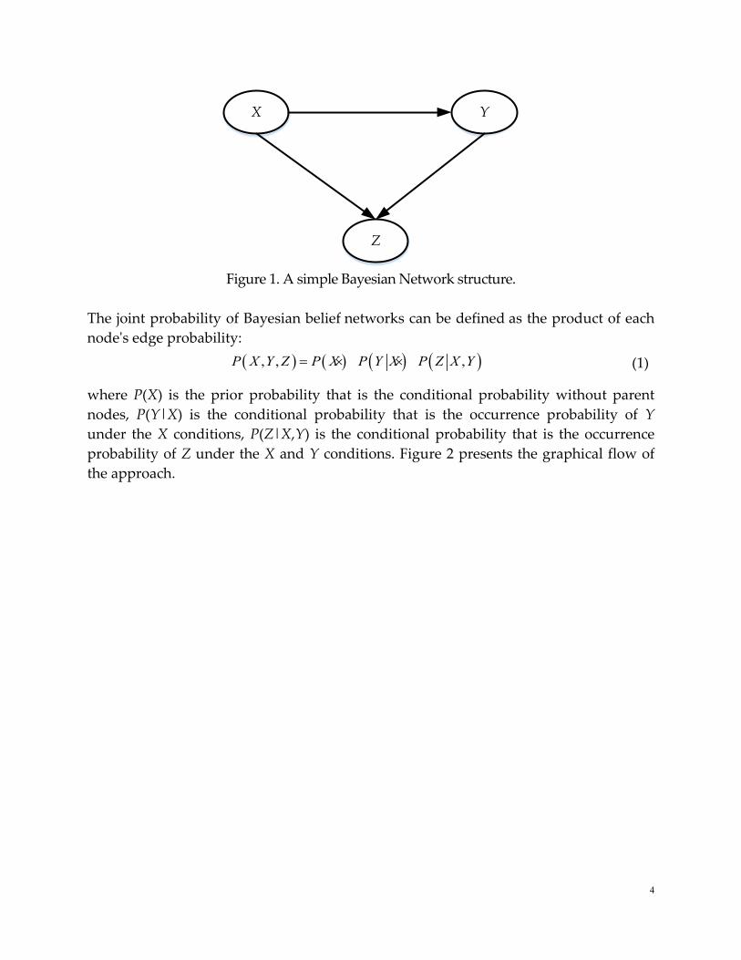
A sample BBN model is shown in Figure 1, where node X is the parent node of the child

nodes Y and Z, and node Y is the parent node of the child node Z. Edges are

represented by the arrows between the two nodes.

4

X Y

Z

Figure 1. A simple Bayesian Network structure.

The joint probability of Bayesian belief networks can be defined as the product of each

node's edge probability:

( ) ( ) ( ) ( ), , ,P X Y Z P X P Y X P Z X Y= × × (1)

where P(X) is the prior probability that is the conditional probability without parent

nodes, P(Y|X) is the conditional probability that is the occurrence probability of Y

under the X conditions, P(Z|X,Y) is the conditional probability that is the occurrence

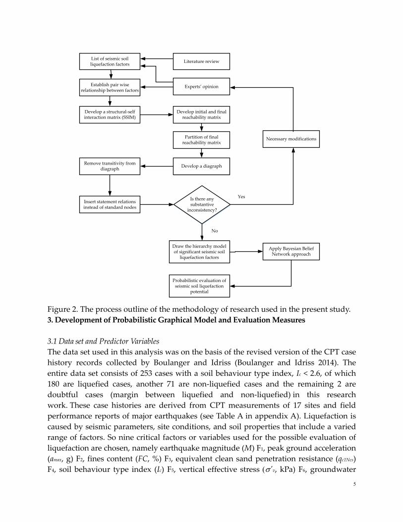
probability of Z under the X and Y conditions. Figure 2 presents the graphical flow of

the approach.

5

Literature reviewList of seismic soil liquefaction factors

Establish pair wise relationship between factors

Experts’ opinion

Develop initial and final reachability matrix

Partition of final reachability matrix

Develop a diagraph

Draw the hierarchy model of significant seismic soil

liquefaction factors

Develop a structural-self interaction matrix (SSIM)

Remove transitivity from diagraph

Insert statement relations instead of standard nodes

Is there any substantive

inconsistency?

Necessary modifications

Yes

No

Apply Bayesian Belief Network approach

Probabilistic evaluation of seismic soil liquefaction

potential

Figure 2. The process outline of the methodology of research used in the present study.

3. Development of Probabilistic Graphical Model and Evaluation Measures

3.1 Data set and Predictor Variables

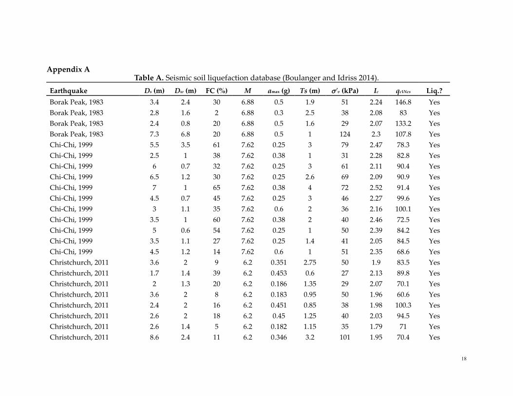
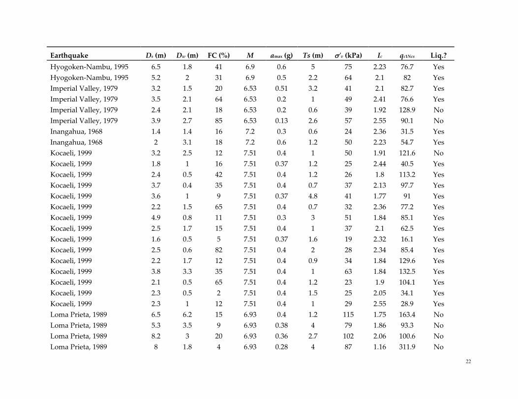
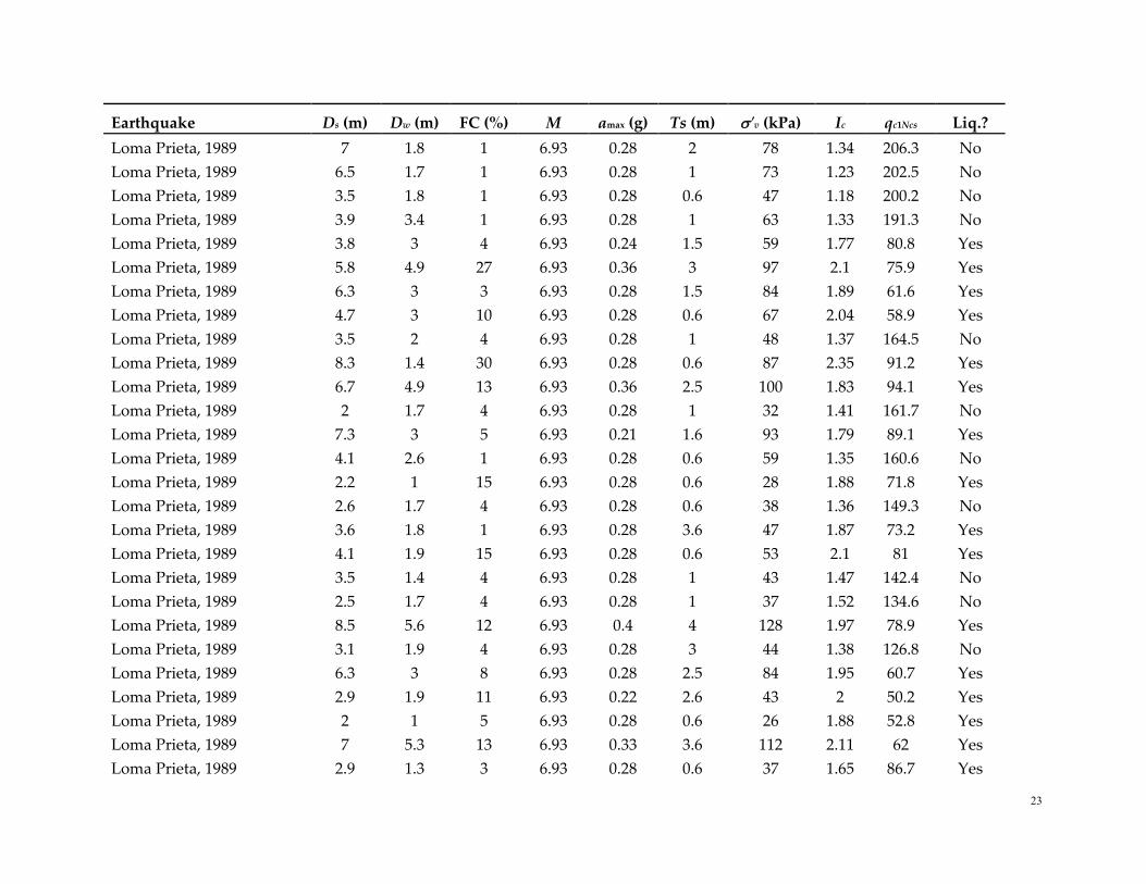
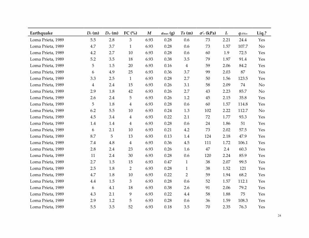
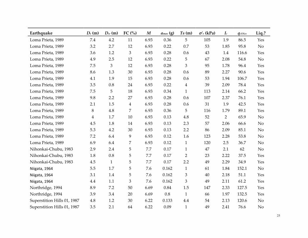
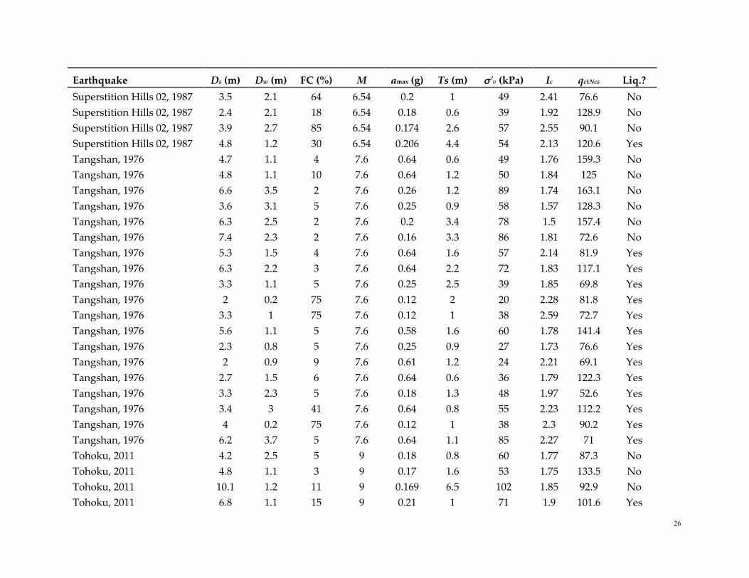
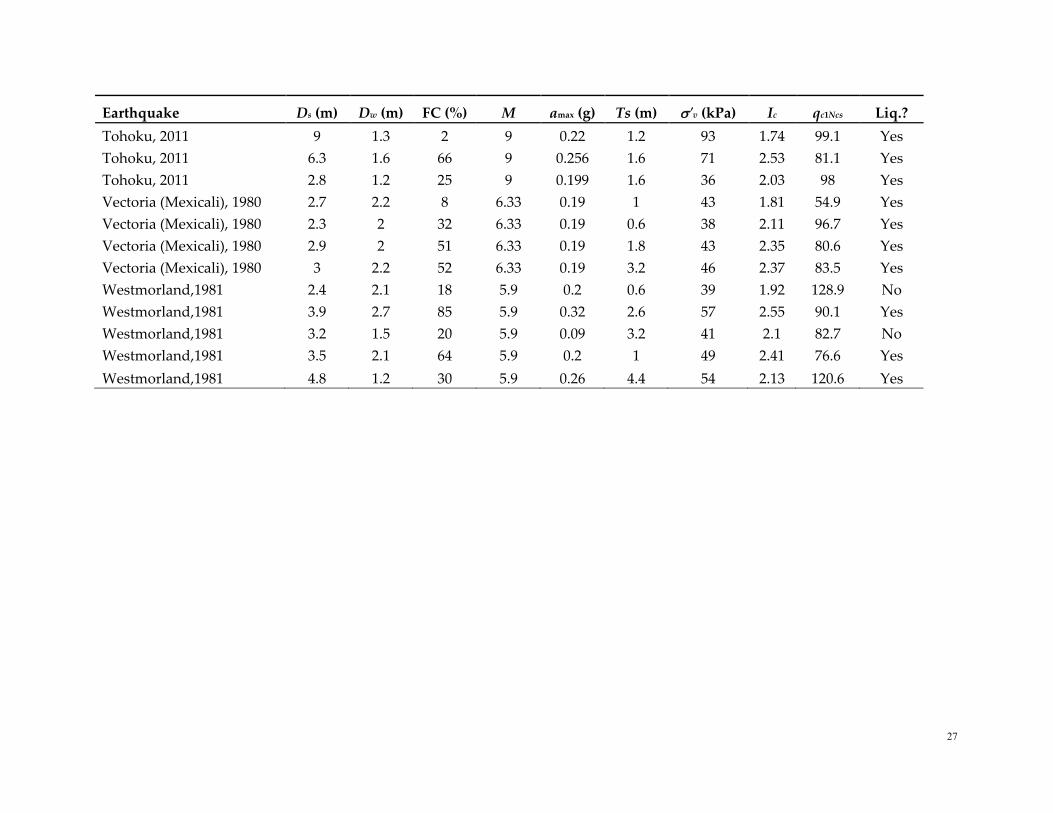
The data set used in this analysis was on the basis of the revised version of the CPT case

history records collected by Boulanger and Idriss (Boulanger and Idriss 2014). The

entire data set consists of 253 cases with a soil behaviour type index, Ic < 2.6, of which

180 are liquefied cases, another 71 are non-liquefied cases and the remaining 2 are

doubtful cases (margin between liquefied and non-liquefied) in this research

work. These case histories are derived from CPT measurements of 17 sites and field

performance reports of major earthquakes (see Table A in appendix A). Liquefaction is

caused by seismic parameters, site conditions, and soil properties that include a varied

range of factors. So nine critical factors or variables used for the possible evaluation of

liquefaction are chosen, namely earthquake magnitude (M) F1, peak ground acceleration

(amax, g) F2, fines content (FC, %) F3, equivalent clean sand penetration resistance (qc1Ncs)

F4, soil behaviour type index (Ic) F5, vertical effective stress (σ'v, kPa) F6, groundwater

6

table depth (Dw, m) F7, depth of soil deposit (Ds, m) F8, thickness of soil layer (Ts, m) F9,

and output is liquefaction potential, F10 in this paper according to Okoli and Schabram

(Okoli and Schabram 2010) and Tranfield et al. (Tranfield et al. 2003). For more details

of CPT case histories, viewers may refer to the Boulanger and Idriss

reference (Boulanger and Idriss 2014). The statistical characteristics of the data set used

in this study, such as minimum (Min.), maximum (Max.), mean, standard deviation

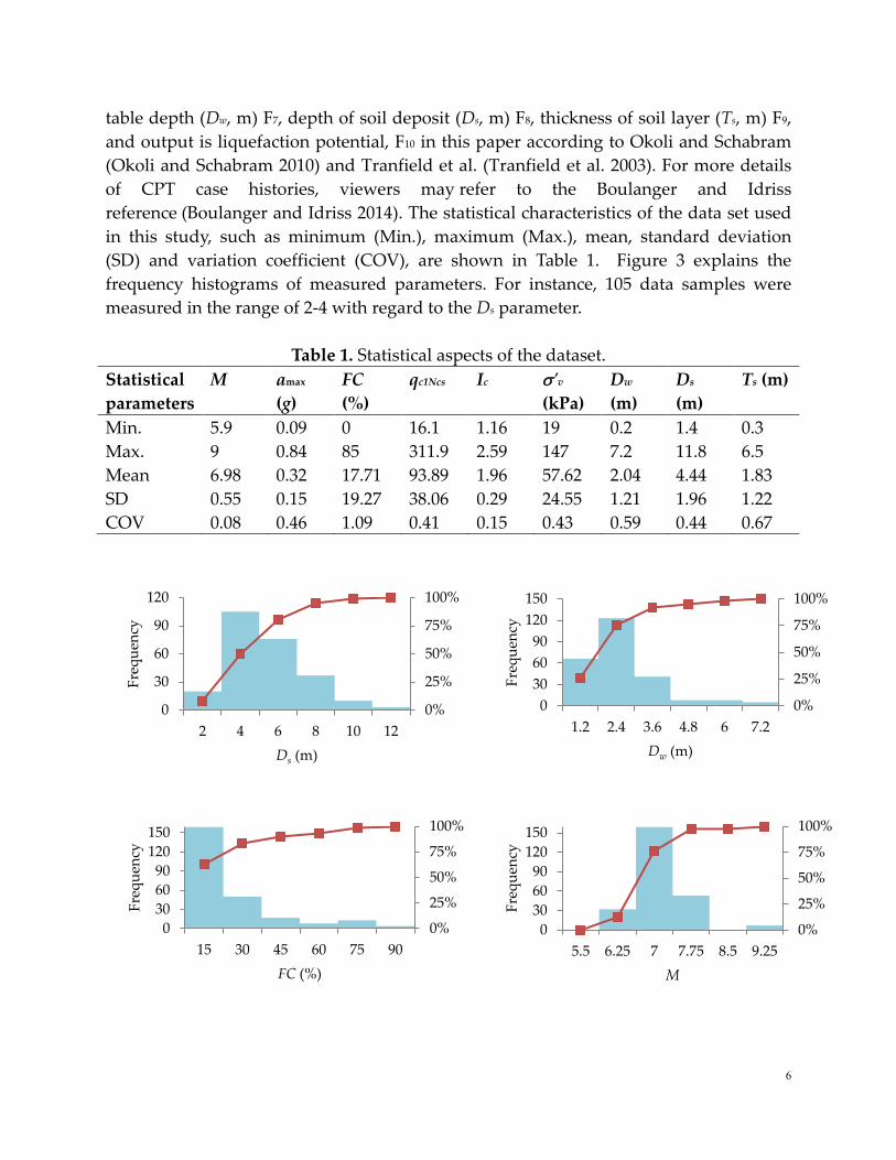
(SD) and variation coefficient (COV), are shown in Table 1. Figure 3 explains the

frequency histograms of measured parameters. For instance, 105 data samples were

measured in the range of 2-4 with regard to the Ds parameter.

Table 1. Statistical aspects of the dataset.

Statistical

parameters

M amax

(g)

FC

(%)

qc1Ncs Ic σ'v

(kPa)

Dw

(m)

Ds

(m)

Ts (m)

Min. 5.9 0.09 0 16.1 1.16 19 0.2 1.4 0.3

Max. 9 0.84 85 311.9 2.59 147 7.2 11.8 6.5

Mean 6.98 0.32 17.71 93.89 1.96 57.62 2.04 4.44 1.83

SD 0.55 0.15 19.27 38.06 0.29 24.55 1.21 1.96 1.22

COV 0.08 0.46 1.09 0.41 0.15 0.43 0.59 0.44 0.67

0%

25%

50%

75%

100%

0

30

60

90

120

2 4 6 8 10 12

Fre

qu

ency

Ds (m)

0%

25%

50%

75%

100%

0

30

60

90

120

150

1.2 2.4 3.6 4.8 6 7.2

Fre

qu

ency

Dw (m)

0%

25%

50%

75%

100%

0

30

60

90

120

150

15 30 45 60 75 90

Fre

qu

ency

FC (%)

0%

25%

50%

75%

100%

0

30

60

90

120

150

5.5 6.25 7 7.75 8.5 9.25

Fre

qu

ency

M

7

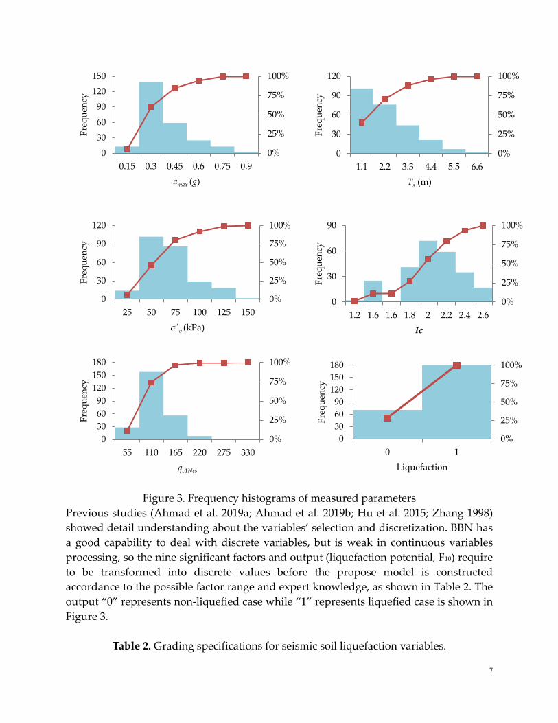
Figure 3. Frequency histograms of measured parameters

Previous studies (Ahmad et al. 2019a; Ahmad et al. 2019b; Hu et al. 2015; Zhang 1998)

showed detail understanding about the variables’ selection and discretization. BBN has

a good capability to deal with discrete variables, but is weak in continuous variables

processing, so the nine significant factors and output (liquefaction potential, F10) require

to be transformed into discrete values before the propose model is constructed

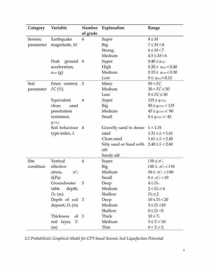
accordance to the possible factor range and expert knowledge, as shown in Table 2. The

output “0” represents non-liquefied case while “1” represents liquefied case is shown in

Figure 3.

Table 2. Grading specifications for seismic soil liquefaction variables.

0%

25%

50%

75%

100%

0

30

60

90

120

150

0.15 0.3 0.45 0.6 0.75 0.9

Fre

qu

ency

amax (g)

0%

25%

50%

75%

100%

0

30

60

90

120

1.1 2.2 3.3 4.4 5.5 6.6

Fre

qu

ency

Ts (m)

0%

25%

50%

75%

100%

0

30

60

90

120

25 50 75 100 125 150

Fre

qu

ency

σ′v (kPa)

0%

25%

50%

75%

100%

0

30

60

90

1.2 1.6 1.6 1.8 2 2.2 2.4 2.6F

req

uen

cyIc

0%

25%

50%

75%

100%

0

30

60

90

120

150

180

55 110 165 220 275 330

Fre

qu

ency

qc1Ncs

0%

25%

50%

75%

100%

0

30

60

90

120

150

180

0 1

Fre

qu

ency

Liquefaction

8

Category Variable Number

of grade

Explanation Range

Seismic

parameter

Earthquake

magnitude, M

4 Super

Big

Strong

Medium

8 ≤ M

7 ≤ M < 8

6 ≤ M < 7

4.5 ≤ M < 6

Peak ground

acceleration,

amax (g)

4 Super

High

Medium

Low

0.40 ≤ amax

0.30 ≤ amax < 0.40

0.15 ≤ amax < 0.30

0 ≤ amax < 0.15

Soil

parameter

Fines content,

FC (%)

3 Many

Medium

Less

50 < FC

30 < FC ≤ 50

0 ≤ FC ≤ 30

Equivalent

clean sand

penetration

resistance,

qc1Ncs

4 Super

Big

Medium

Small

135 ≤ qc1Ncs

90 ≤ qc1Ncs < 135

45 ≤ qc1Ncs < 90

0 ≤ qc1Ncs < 45

Soil behaviour

type index, Ic

4 Gravelly sand to dense

sand

Clean sand

Silty sand or Sand with

silt

Sandy silt

Ic < 1.31

1.31 ≤ Ic < 1.61

1.61 ≤ Ic < 2.40

2.40 ≤ Ic < 2.60

Site

condition

Vertical

effective

stress, σ'v

(kPa)

4 Super

Big

Medium

Small

150 ≤ σ'v 100 ≤ σ'v < 150 50 ≤ σ'v < 100 0 ≤ σ'v < 50

Groundwater

table depth,

Dw (m)

3 Deep

Medium

Shallow

4 ≤ Dw

2 < Dw < 4

Dw ≤ 2

Depth of soil

deposit, Ds (m)

3 Deep

Medium

Shallow

10 ≤ Ds < 20

5 ≤ Ds <10

0 ≤ Ds <5

Thickness of

soil layer, Ts

(m)

3 Thick

Medium

Thin

10 ≤ Ts

5 ≤ Ts < 10

0 < Ts < 5

3.2 Probabilistic Graphical Model for CPT-based Seismic Soil Liquefaction Potential

9

The data set has been divided into training and testing datasets according to statistical

aspects for example mean, maximum, minimum, etc. to build the models:

To build the models, a training data set is required. In this study, 201 (80%) CPT

case histories of the data were used by authors for training set.

To predict the performance of the established models, a testing data set is

required. In this study, the remaining 50 (20%) CPT case histories data is

considered to be a testing data set.

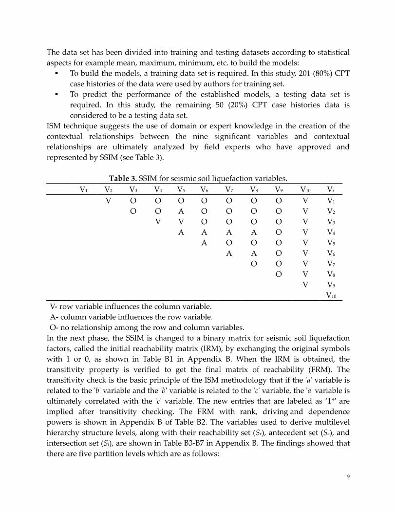
ISM technique suggests the use of domain or expert knowledge in the creation of the

contextual relationships between the nine significant variables and contextual

relationships are ultimately analyzed by field experts who have approved and

represented by SSIM (see Table 3).

Table 3. SSIM for seismic soil liquefaction variables. V1 V2 V3 V4 V5 V6 V7 V8 V9 V10 Vi

V O O O O O O O V V1 O O A O O O O V V2 V V O O O O V V3 A A A A O V V4 A O O O V V5 A A O V V6 O O V V7 O V V8 V V9 V10

V- row variable influences the column variable.

A- column variable influences the row variable.

O- no relationship among the row and column variables.

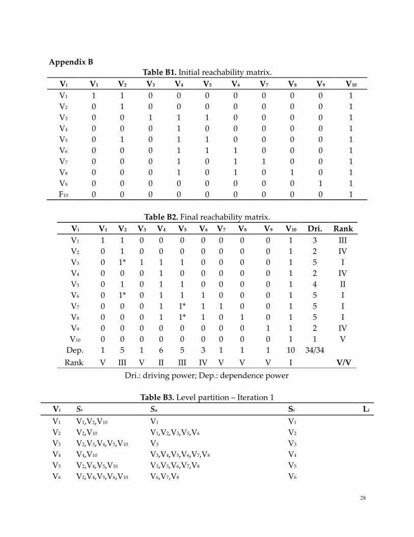
In the next phase, the SSIM is changed to a binary matrix for seismic soil liquefaction

factors, called the initial reachability matrix (IRM), by exchanging the original symbols

with 1 or 0, as shown in Table B1 in Appendix B. When the IRM is obtained, the

transitivity property is verified to get the final matrix of reachability (FRM). The

transitivity check is the basic principle of the ISM methodology that if the 'a' variable is

related to the 'b' variable and the 'b' variable is related to the 'c' variable, the 'a' variable is

ultimately correlated with the 'c' variable. The new entries that are labeled as ‘1*’ are

implied after transitivity checking. The FRM with rank, driving and dependence

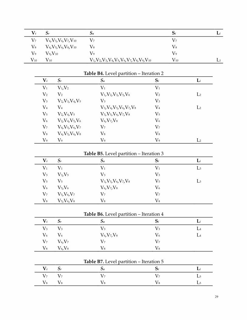
powers is shown in Appendix B of Table B2. The variables used to derive multilevel

hierarchy structure levels, along with their reachability set (Sr), antecedent set (Sa), and

intersection set (Si), are shown in Table B3-B7 in Appendix B. The findings showed that

there are five partition levels which are as follows:

10

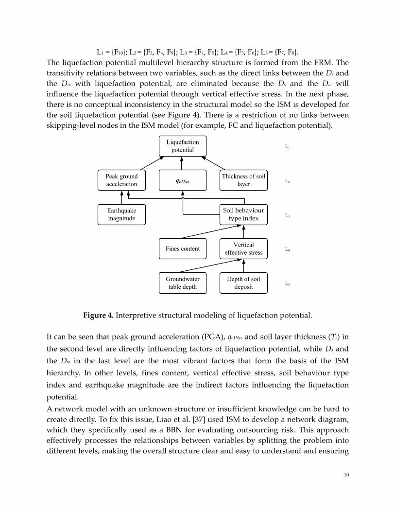
L1 = {F10}; L2 = {F2, F4, F9}; L3 = {F1, F5}; L4 = {F3, F6}; L5 = {F7, F8}.

The liquefaction potential multilevel hierarchy structure is formed from the FRM. The

transitivity relations between two variables, such as the direct links between the Ds and

the Dw with liquefaction potential, are eliminated because the Ds and the Dw will

influence the liquefaction potential through vertical effective stress. In the next phase,

there is no conceptual inconsistency in the structural model so the ISM is developed for

the soil liquefaction potential (see Figure 4). There is a restriction of no links between

skipping-level nodes in the ISM model (for example, FC and liquefaction potential).

Fines contentVertical

effective stress

Earthquake

magnitude

Soil behaviour type index

Peak ground

accelerationqc1Ncs

Groundwater

table depth

Depth of soil

deposit

Thickness of soil

layer

Liquefaction

potentialL1

L2

L3

L4

L5

Figure 4. Interpretive structural modeling of liquefaction potential.

It can be seen that peak ground acceleration (PGA), qc1Ncs and soil layer thickness (Ts) in

the second level are directly influencing factors of liquefaction potential, while Ds and

the Dw in the last level are the most vibrant factors that form the basis of the ISM

hierarchy. In other levels, fines content, vertical effective stress, soil behaviour type

index and earthquake magnitude are the indirect factors influencing the liquefaction

potential.

A network model with an unknown structure or insufficient knowledge can be hard to

create directly. To fix this issue, Liao et al. [37] used ISM to develop a network diagram,

which they specifically used as a BBN for evaluating outsourcing risk. This approach

effectively processes the relationships between variables by splitting the problem into

different levels, making the overall structure clear and easy to understand and ensuring

11

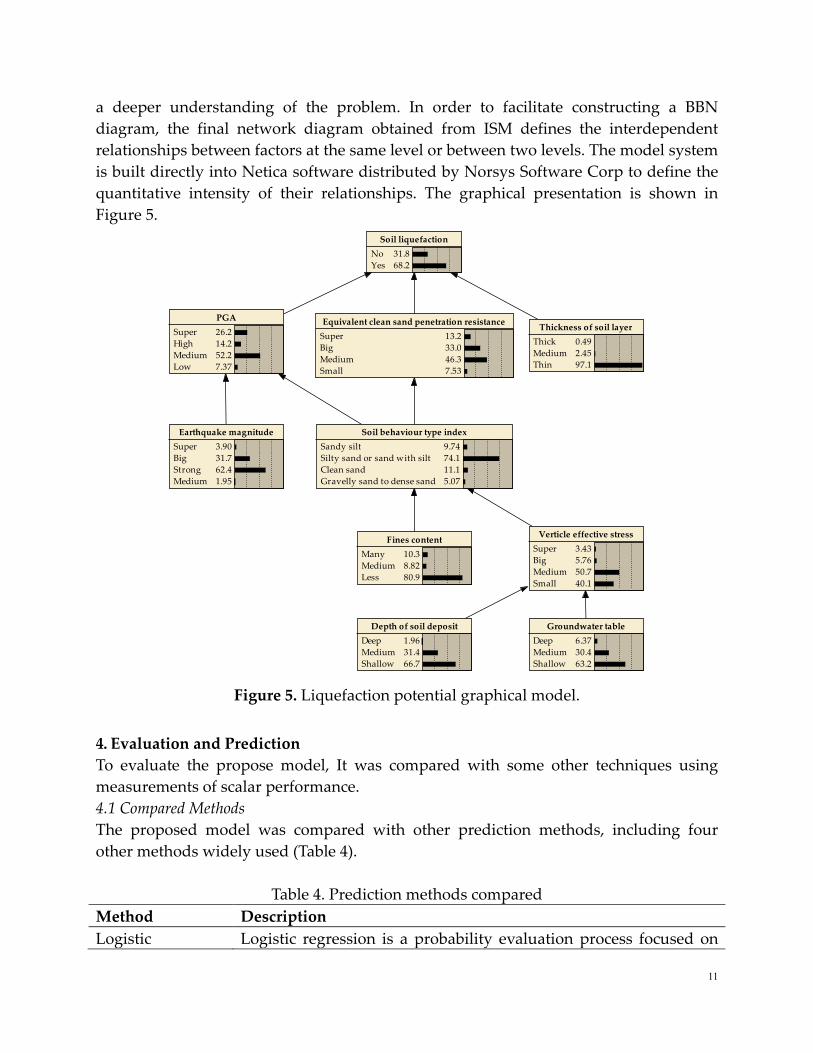
a deeper understanding of the problem. In order to facilitate constructing a BBN

diagram, the final network diagram obtained from ISM defines the interdependent

relationships between factors at the same level or between two levels. The model system

is built directly into Netica software distributed by Norsys Software Corp to define the

quantitative intensity of their relationships. The graphical presentation is shown in

Figure 5.

Figure 5. Liquefaction potential graphical model.

4. Evaluation and Prediction

To evaluate the propose model, It was compared with some other techniques using

measurements of scalar performance.

4.1 Compared Methods

The proposed model was compared with other prediction methods, including four

other methods widely used (Table 4).

Table 4. Prediction methods compared

Method Description

Logistic Logistic regression is a probability evaluation process focused on

Groundwater table

Deep

Medium

Shallow

6.37

30.4

63.2

Verticle effective stress

Super

Big

Medium

Small

3.43

5.76

50.7

40.1

Earthquake magnitude

Super

Big

Strong

Medium

3.90

31.7

62.4

1.95

Soil liquefaction

No

Yes

31.8

68.2

Thickness of soil layer

Thick

Medium

Thin

0.49

2.45

97.1

PGA

Super

High

Medium

Low

26.2

14.2

52.2

7.37

Equivalent clean sand penetration resistance

Super

Big

Medium

Small

13.2

33.0

46.3

7.53


Sandy silt

Silty sand or sand with silt

Clean sand

Gravelly sand to dense sand

9.74

74.1

11.1

5.07

Fines content

Many

Medium

Less

10.3

8.82

80.9

Depth of soil deposit

Deep

Medium

Shallow

1.96

31.4

66.7

12

Method Description

Regression (LR) the calculation of maximum probability (Hosmer and Lemeshow

2000).

Support Vector

Machine (SVM)

SVM, based on mathematical learning models is one of the most

robust prediction methods (Vapnik 1995). SVM training method

computes a model that assigns new examples to one category or

the other, making it a non-probabilistic binary linear classifier,

given a set of training examples, each marked as belonging to one

of two categories.

Random Forest

(RF)

Random forest (Breiman 2001) is a meta-learning scheme that

integrates many independently developed base classifiers and

participates in a voting process to obtain a prediction for the final

class.

Naive Bayes (NB) Naive Bayes (John and Langley 1995) assumes that the predictive

variables, provided the target/dependent variable, are conditionally

independent.

4.2 Evaluation Measures

Four scalar measurements are used, i.e., accuracy, precision, recall and F-measure. There

are four possible outcomes for a single prediction in the binary class scenario, i.e.,

liquefaction and non-liquefaction. The correct classification is true negative (TN) and

true positive (TP). If the output is incorrectly predicted as negative, a false positive (FP)

occurs, If the result is wrongly labeled as negative, a false negative (FN) occurs.

Accuracy (acc) is a calculation of the total number of accurate predictions. The acc's

value is calculated as follows:

TP TNacc

TP FN FP TN

+=

+ + + (2)

Precision refers to the proportion of correctly classified positive cases and recall is

referred to as the portion of correctly classified actual positive cases. A pair of

contradictory measures is precision (pr) and recall (re). The pr is generally large, while re

is not large, or vice versa. The confusion matrix (see Table 5) can be used to evaluate

these as:

TP TNpr or

TP FP FN TN=

+ + (3)

TP TNre or

TP FN FP TN=

+ + (4)

13

2 pr reF score

pr re

× ×− =

+ (5)

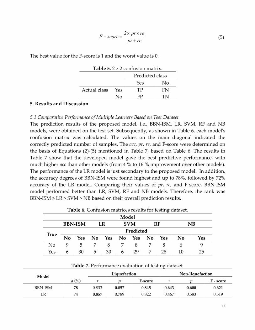
The best value for the F-score is 1 and the worst value is 0.

Table 5. 2 × 2 confusion matrix.

Predicted class

Yes No

Actual class Yes TP FN

No FP TN

5. Results and Discussion

5.1 Comparative Performance of Multiple Learners Based on Test Dataset

The prediction results of the proposed model, i.e., BBN-ISM, LR, SVM, RF and NB

models, were obtained on the test set. Subsequently, as shown in Table 6, each model's

confusion matrix was calculated. The values on the main diagonal indicated the

correctly predicted number of samples. The acc, pr, re, and F-score were determined on

the basis of Equations (2)-(5) mentioned in Table 7, based on Table 6. The results in

Table 7 show that the developed model gave the best predictive performance, with

much higher acc than other models (from 4 % to 16 % improvement over other models).

The performance of the LR model is just secondary to the proposed model. In addition,

the accuracy degrees of BBN-ISM were found highest and up to 78%, followed by 72%

accuracy of the LR model. Comparing their values of pr, re, and F-score, BBN-ISM

model performed better than LR, SVM, RF and NB models. Therefore, the rank was

BBN-ISM > LR > SVM > NB based on their overall prediction results.

Table 6. Confusion matrices results for testing dataset.

Model

BBN-ISM LR SVM RF NB

True Predicted

No Yes No Yes No Yes No Yes No Yes

No 9 5 7 8 7 8 7 8 6 9

Yes 6 30 5 30 6 29 7 28 10 25

Table 7. Performance evaluation of testing dataset.

Model Liquefaction Non-liquefaction

a (%) r p F-score r p F - score

BBN-ISM 78 0.833 0.857 0.845 0.643 0.600 0.621

LR 74 0.857 0.789 0.822 0.467 0.583 0.519

14

Model Liquefaction Non-liquefaction

a (%) r p F-score r p F - score

SVM 72 0.829 0.784 0.806 0.467 0.538 0.500

RF 70 0.800 0.778 0.789 0.467 0.500 0.483

Naïve Bayes 62 0.714 0.735 0.725 0.400 0.375 0.387

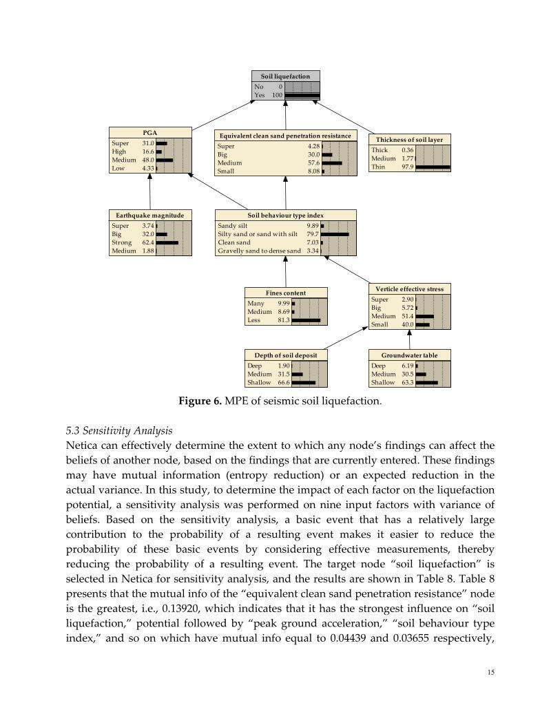
5.2 Most Probable Explanation

Using the Netica function to decide which situation is most probable to cause soil

liquefaction potential, the most probable explanation (MPE) can be found and the

established model can be used to obtain the most probable explanation. For instance, if

the soil liquefaction is "yes" as shown in Figure 6, the function "most probable

explanation" is used to identify the set that is most probable to cause "soil liquefaction"

which is [peak ground acceleration = medium, equivalent clean sand penetration

resistance = medium, thickness of soil layer = thin, earthquake magnitude = strong, soil

behaviour type index = silty sand, fines content = less, vertical effective stress = small,

groundwater table = shallow, and depth of soil deposit = shallow]. This shows explicitly

that the set is indeed well associated with the judgment of engineering.

15

Figure 6. MPE of seismic soil liquefaction.

5.3 Sensitivity Analysis

Netica can effectively determine the extent to which any node’s findings can affect the

beliefs of another node, based on the findings that are currently entered. These findings

may have mutual information (entropy reduction) or an expected reduction in the

actual variance. In this study, to determine the impact of each factor on the liquefaction

potential, a sensitivity analysis was performed on nine input factors with variance of

beliefs. Based on the sensitivity analysis, a basic event that has a relatively large

contribution to the probability of a resulting event makes it easier to reduce the

probability of these basic events by considering effective measurements, thereby

reducing the probability of a resulting event. The target node “soil liquefaction” is

selected in Netica for sensitivity analysis, and the results are shown in Table 8. Table 8

presents that the mutual info of the “equivalent clean sand penetration resistance” node

is the greatest, i.e., 0.13920, which indicates that it has the strongest influence on “soil

liquefaction,” potential followed by “peak ground acceleration,” “soil behaviour type

index,” and so on which have mutual info equal to 0.04439 and 0.03655 respectively,

Groundwater table

Deep

Medium

Shallow

6.19

30.5

63.3

Verticle effective stress

Super

Big

Medium

Small

2.90

5.72

51.4

40.0

Earthquake magnitude

Super

Big

Strong

Medium

3.74

32.0

62.4

1.88

Soil liquefaction

No

Yes

0

100

Thickness of soil layer

Thick

Medium

Thin

0.36

1.77

97.9

PGA

Super

High

Medium

Low

31.0

16.6

48.0

4.33

Equivalent clean sand penetration resistance

Super

Big

Medium

Small

4.28

30.0

57.6

8.08


Sandy silt

Silty sand or sand with silt

Clean sand

Gravelly sand to dense sand

9.89

79.7

7.03

3.34

Fines content

Many

Medium

Less

9.99

8.69

81.3

Depth of soil deposit

Deep

Medium

Shallow

1.90

31.5

66.6

16

whereas the “depth of soil deposit” is bared minimum sensitive factor with a mutual

info equal to 0.00004; those findings are strongly consistent with the literature.

Table 8. Sensitivity analysis of “soil liquefaction” node. Node qc1Ncs amax (g) Ic Ts (m) σ'v (kPa) FC (%) M Dw (m) Ds (m)

Mutual info 0.13920 0.04439 0.03655 0.00334 0.00135 0.00021 0.00019 0.00009 0.00004

Percent 15.4000 4.9200 4.0500 0.3700 0.1490 0.0234 0.0212 0.0101 0.0047

Variance of

beliefs

0.0423618 0.0133434 0.0117117 0.0010781 0.0004219 0.0000640 0.0000581 0.0000275 0.0000128

6. Conclusions and Future Prospect

In this paper, probabilistic evaluation of CPT-based seismic soil liquefaction was carried

by systematically integrating ISM and the BBN. The models were trained and tested

based on Boulanger and Idriss database compiles from various soil liquefaction in

different countries. The proposed model predicts the seismic soil liquefaction using

major contributing factors on soil liquefaction. The most important conclusions of the

present research work are as follows:

1. The accuracy of the proposed model is 78% and the F-score is 0.845 for

liquefaction data and 0.621 for non-liquefaction data. In comparison with LR,

SVM, RF, and NB models, the proposed model has better prediction ability and,

because of a simple graphical result, its implementation is simpler.

2. The MPE of seismic soil liquefaction is that the peak ground acceleration =

medium, equivalent clean sand penetration resistance = medium, thickness of

soil layer = thin, earthquake magnitude = strong, soil behaviour type index = silty

sand, fines content = less, vertical effective stress = small, groundwater table =

shallow, and depth of soil deposit = shallow, which suits well in accordance with

engineering practice.

3. Sensitivity analysis shows the most important parameters on the soil

liquefaction: qc1Ncs and PGA determine the strongest, followed by Ic, Ts, σ′v, FC, M,

Dw, and Ds. It is probably due to the fact that the variation of these parameters is

not very much.

Since the CPT case histories database have class imbalanced and the sampling biased in

training and testing data set may lead anecdotal results to some degree. Nevertheless,

these anecdotal findings regarding seismic soil liquefaction potential evaluation are

greatly insightful from a preliminary viewpoint. In addition, owing to the ISM

shortcomings, such as ignoring relationships between the nodes of the skipping-level,

and there is no feedback circuit between any two levels, some significant node

relationships will be ignored. In the future, the causal mapping approach should be

employed to change the structure and to refine the prediction performance results,

taking into account the ISM shortcomings.

17

Acknowledgments

The authors would like to thank the experts who participated in the modeling process.

The research described in this paper was part of research sponsored by the National

Key Research & Development Plan of China (Grant Nos. 2018YFC1505305 and

2016YFE0200100) and Key Program of National Natural Science Foundation of China

(Grant No. 51639002).

18

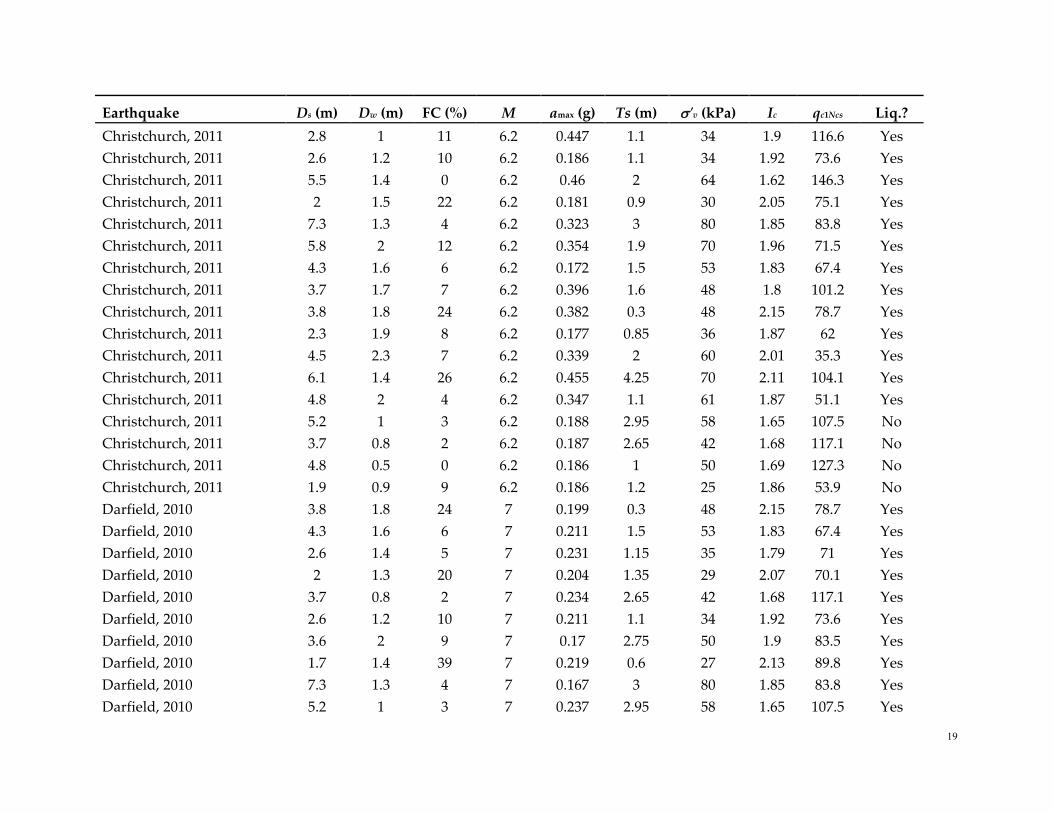
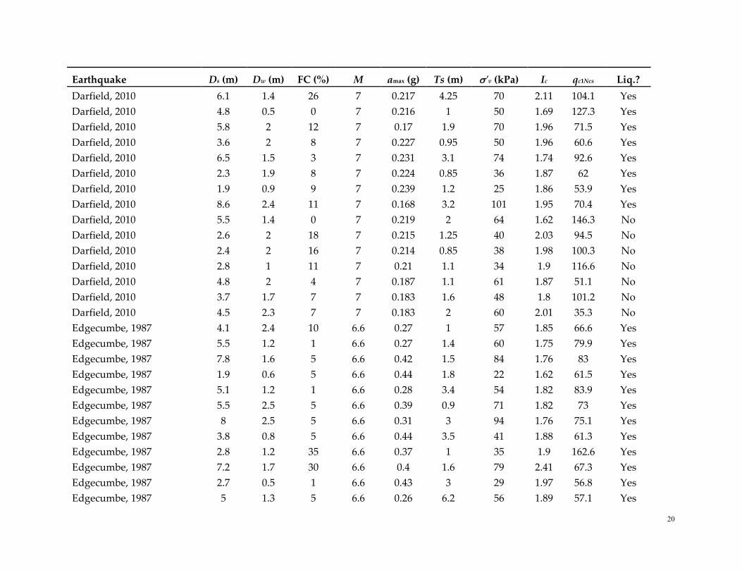
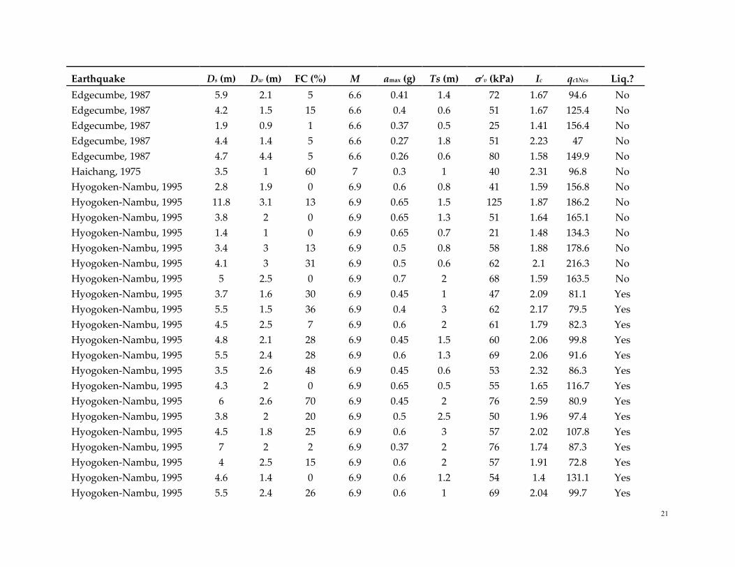
Appendix A

Table A. Seismic soil liquefaction database (Boulanger and Idriss 2014).

Earthquake Ds (m) Dw (m) FC (%) M amax (g) Ts (m) σ'v (kPa) Ic qc1Ncs Liq.?

Borak Peak, 1983 3.4 2.4 30 6.88 0.5 1.9 51 2.24 146.8 Yes

Borak Peak, 1983 2.8 1.6 2 6.88 0.3 2.5 38 2.08 83 Yes

Borak Peak, 1983 2.4 0.8 20 6.88 0.5 1.6 29 2.07 133.2 Yes

Borak Peak, 1983 7.3 6.8 20 6.88 0.5 1 124 2.3 107.8 Yes

Chi-Chi, 1999 5.5 3.5 61 7.62 0.25 3 79 2.47 78.3 Yes

Chi-Chi, 1999 2.5 1 38 7.62 0.38 1 31 2.28 82.8 Yes

Chi-Chi, 1999 6 0.7 32 7.62 0.25 3 61 2.11 90.4 Yes

Chi-Chi, 1999 6.5 1.2 30 7.62 0.25 2.6 69 2.09 90.9 Yes

Chi-Chi, 1999 7 1 65 7.62 0.38 4 72 2.52 91.4 Yes

Chi-Chi, 1999 4.5 0.7 45 7.62 0.25 3 46 2.27 99.6 Yes

Chi-Chi, 1999 3 1.1 35 7.62 0.6 2 36 2.16 100.1 Yes

Chi-Chi, 1999 3.5 1 60 7.62 0.38 2 40 2.46 72.5 Yes

Chi-Chi, 1999 5 0.6 54 7.62 0.25 1 50 2.39 84.2 Yes

Chi-Chi, 1999 3.5 1.1 27 7.62 0.25 1.4 41 2.05 84.5 Yes

Chi-Chi, 1999 4.5 1.2 14 7.62 0.6 1 51 2.35 68.6 Yes

Christchurch, 2011 3.6 2 9 6.2 0.351 2.75 50 1.9 83.5 Yes

Christchurch, 2011 1.7 1.4 39 6.2 0.453 0.6 27 2.13 89.8 Yes

Christchurch, 2011 2 1.3 20 6.2 0.186 1.35 29 2.07 70.1 Yes




Christchurch, 2011 2.6 1.4 5 6.2 0.182 1.15 35 1.79 71 Yes


19




Christchurch, 2011 5.5 1.4 0 6.2 0.46 2 64 1.62 146.3 Yes

Christchurch, 2011 2 1.5 22 6.2 0.181 0.9 30 2.05 75.1 Yes






Christchurch, 2011 2.3 1.9 8 6.2 0.177 0.85 36 1.87 62 Yes




Christchurch, 2011 5.2 1 3 6.2 0.188 2.95 58 1.65 107.5 No

Christchurch, 2011 3.7 0.8 2 6.2 0.187 2.65 42 1.68 117.1 No

Christchurch, 2011 4.8 0.5 0 6.2 0.186 1 50 1.69 127.3 No

Christchurch, 2011 1.9 0.9 9 6.2 0.186 1.2 25 1.86 53.9 No

Darfield, 2010 3.8 1.8 24 7 0.199 0.3 48 2.15 78.7 Yes

Darfield, 2010 4.3 1.6 6 7 0.211 1.5 53 1.83 67.4 Yes

Darfield, 2010 2.6 1.4 5 7 0.231 1.15 35 1.79 71 Yes

Darfield, 2010 2 1.3 20 7 0.204 1.35 29 2.07 70.1 Yes

Darfield, 2010 3.7 0.8 2 7 0.234 2.65 42 1.68 117.1 Yes

Darfield, 2010 2.6 1.2 10 7 0.211 1.1 34 1.92 73.6 Yes

Darfield, 2010 3.6 2 9 7 0.17 2.75 50 1.9 83.5 Yes

Darfield, 2010 1.7 1.4 39 7 0.219 0.6 27 2.13 89.8 Yes

Darfield, 2010 7.3 1.3 4 7 0.167 3 80 1.85 83.8 Yes

Darfield, 2010 5.2 1 3 7 0.237 2.95 58 1.65 107.5 Yes

20


Darfield, 2010 6.1 1.4 26 7 0.217 4.25 70 2.11 104.1 Yes

Darfield, 2010 4.8 0.5 0 7 0.216 1 50 1.69 127.3 Yes

Darfield, 2010 5.8 2 12 7 0.17 1.9 70 1.96 71.5 Yes

Darfield, 2010 3.6 2 8 7 0.227 0.95 50 1.96 60.6 Yes

Darfield, 2010 6.5 1.5 3 7 0.231 3.1 74 1.74 92.6 Yes

Darfield, 2010 2.3 1.9 8 7 0.224 0.85 36 1.87 62 Yes

Darfield, 2010 1.9 0.9 9 7 0.239 1.2 25 1.86 53.9 Yes

Darfield, 2010 8.6 2.4 11 7 0.168 3.2 101 1.95 70.4 Yes

Darfield, 2010 5.5 1.4 0 7 0.219 2 64 1.62 146.3 No

Darfield, 2010 2.6 2 18 7 0.215 1.25 40 2.03 94.5 No

Darfield, 2010 2.4 2 16 7 0.214 0.85 38 1.98 100.3 No

Darfield, 2010 2.8 1 11 7 0.21 1.1 34 1.9 116.6 No

Darfield, 2010 4.8 2 4 7 0.187 1.1 61 1.87 51.1 No

Darfield, 2010 3.7 1.7 7 7 0.183 1.6 48 1.8 101.2 No

Darfield, 2010 4.5 2.3 7 7 0.183 2 60 2.01 35.3 No

Edgecumbe, 1987 4.1 2.4 10 6.6 0.27 1 57 1.85 66.6 Yes

Edgecumbe, 1987 5.5 1.2 1 6.6 0.27 1.4 60 1.75 79.9 Yes

Edgecumbe, 1987 7.8 1.6 5 6.6 0.42 1.5 84 1.76 83 Yes

Edgecumbe, 1987 1.9 0.6 5 6.6 0.44 1.8 22 1.62 61.5 Yes

Edgecumbe, 1987 5.1 1.2 1 6.6 0.28 3.4 54 1.82 83.9 Yes

Edgecumbe, 1987 5.5 2.5 5 6.6 0.39 0.9 71 1.82 73 Yes

Edgecumbe, 1987 8 2.5 5 6.6 0.31 3 94 1.76 75.1 Yes

Edgecumbe, 1987 3.8 0.8 5 6.6 0.44 3.5 41 1.88 61.3 Yes

Edgecumbe, 1987 2.8 1.2 35 6.6 0.37 1 35 1.9 162.6 Yes

Edgecumbe, 1987 7.2 1.7 30 6.6 0.4 1.6 79 2.41 67.3 Yes

Edgecumbe, 1987 2.7 0.5 1 6.6 0.43 3 29 1.97 56.8 Yes

Edgecumbe, 1987 5 1.3 5 6.6 0.26 6.2 56 1.89 57.1 Yes

21


Edgecumbe, 1987 5.9 2.1 5 6.6 0.41 1.4 72 1.67 94.6 No

Edgecumbe, 1987 4.2 1.5 15 6.6 0.4 0.6 51 1.67 125.4 No

Edgecumbe, 1987 1.9 0.9 1 6.6 0.37 0.5 25 1.41 156.4 No

Edgecumbe, 1987 4.4 1.4 5 6.6 0.27 1.8 51 2.23 47 No

Edgecumbe, 1987 4.7 4.4 5 6.6 0.26 0.6 80 1.58 149.9 No

Haichang, 1975 3.5 1 60 7 0.3 1 40 2.31 96.8 No

Hyogoken-Nambu, 1995 2.8 1.9 0 6.9 0.6 0.8 41 1.59 156.8 No

Hyogoken-Nambu, 1995 11.8 3.1 13 6.9 0.65 1.5 125 1.87 186.2 No

Hyogoken-Nambu, 1995 3.8 2 0 6.9 0.65 1.3 51 1.64 165.1 No




Hyogoken-Nambu, 1995 5 2.5 0 6.9 0.7 2 68 1.59 163.5 No

Hyogoken-Nambu, 1995 3.7 1.6 30 6.9 0.45 1 47 2.09 81.1 Yes



Hyogoken-Nambu, 1995 4.8 2.1 28 6.9 0.45 1.5 60 2.06 99.8 Yes



Hyogoken-Nambu, 1995 4.3 2 0 6.9 0.65 0.5 55 1.65 116.7 Yes

Hyogoken-Nambu, 1995 6 2.6 70 6.9 0.45 2 76 2.59 80.9 Yes

Hyogoken-Nambu, 1995 3.8 2 20 6.9 0.5 2.5 50 1.96 97.4 Yes


Hyogoken-Nambu, 1995 7 2 2 6.9 0.37 2 76 1.74 87.3 Yes

Hyogoken-Nambu, 1995 4 2.5 15 6.9 0.6 2 57 1.91 72.8 Yes



22



Hyogoken-Nambu, 1995 5.2 2 31 6.9 0.5 2.2 64 2.1 82 Yes

Imperial Valley, 1979 3.2 1.5 20 6.53 0.51 3.2 41 2.1 82.7 Yes

Imperial Valley, 1979 3.5 2.1 64 6.53 0.2 1 49 2.41 76.6 Yes

Imperial Valley, 1979 2.4 2.1 18 6.53 0.2 0.6 39 1.92 128.9 No

Imperial Valley, 1979 3.9 2.7 85 6.53 0.13 2.6 57 2.55 90.1 No

Inangahua, 1968 1.4 1.4 16 7.2 0.3 0.6 24 2.36 31.5 Yes

Inangahua, 1968 2 3.1 18 7.2 0.6 1.2 50 2.23 54.7 Yes

Kocaeli, 1999 3.2 2.5 12 7.51 0.4 1 50 1.91 121.6 No

Kocaeli, 1999 1.8 1 16 7.51 0.37 1.2 25 2.44 40.5 Yes

Kocaeli, 1999 2.4 0.5 42 7.51 0.4 1.2 26 1.8 113.2 Yes

Kocaeli, 1999 3.7 0.4 35 7.51 0.4 0.7 37 2.13 97.7 Yes

Kocaeli, 1999 3.6 1 9 7.51 0.37 4.8 41 1.77 91 Yes

Kocaeli, 1999 2.2 1.5 65 7.51 0.4 0.7 32 2.36 77.2 Yes

Kocaeli, 1999 4.9 0.8 11 7.51 0.3 3 51 1.84 85.1 Yes

Kocaeli, 1999 2.5 1.7 15 7.51 0.4 1 37 2.1 62.5 Yes

Kocaeli, 1999 1.6 0.5 5 7.51 0.37 1.6 19 2.32 16.1 Yes

Kocaeli, 1999 2.5 0.6 82 7.51 0.4 2 28 2.34 85.4 Yes

Kocaeli, 1999 2.2 1.7 12 7.51 0.4 0.9 34 1.84 129.6 Yes

Kocaeli, 1999 3.8 3.3 35 7.51 0.4 1 63 1.84 132.5 Yes

Kocaeli, 1999 2.1 0.5 65 7.51 0.4 1.2 23 1.9 104.1 Yes

Kocaeli, 1999 2.3 0.5 2 7.51 0.4 1.5 25 2.05 34.1 Yes

Kocaeli, 1999 2.3 1 12 7.51 0.4 1 29 2.55 28.9 Yes

Loma Prieta, 1989 6.5 6.2 15 6.93 0.4 1.2 115 1.75 163.4 No

Loma Prieta, 1989 5.3 3.5 9 6.93 0.38 4 79 1.86 93.3 No

Loma Prieta, 1989 8.2 3 20 6.93 0.36 2.7 102 2.06 100.6 No

Loma Prieta, 1989 8 1.8 4 6.93 0.28 4 87 1.16 311.9 No

23


Loma Prieta, 1989 7 1.8 1 6.93 0.28 2 78 1.34 206.3 No

Loma Prieta, 1989 6.5 1.7 1 6.93 0.28 1 73 1.23 202.5 No

Loma Prieta, 1989 3.5 1.8 1 6.93 0.28 0.6 47 1.18 200.2 No

Loma Prieta, 1989 3.9 3.4 1 6.93 0.28 1 63 1.33 191.3 No

Loma Prieta, 1989 3.8 3 4 6.93 0.24 1.5 59 1.77 80.8 Yes

Loma Prieta, 1989 5.8 4.9 27 6.93 0.36 3 97 2.1 75.9 Yes

Loma Prieta, 1989 6.3 3 3 6.93 0.28 1.5 84 1.89 61.6 Yes

Loma Prieta, 1989 4.7 3 10 6.93 0.28 0.6 67 2.04 58.9 Yes

Loma Prieta, 1989 3.5 2 4 6.93 0.28 1 48 1.37 164.5 No

Loma Prieta, 1989 8.3 1.4 30 6.93 0.28 0.6 87 2.35 91.2 Yes

Loma Prieta, 1989 6.7 4.9 13 6.93 0.36 2.5 100 1.83 94.1 Yes

Loma Prieta, 1989 2 1.7 4 6.93 0.28 1 32 1.41 161.7 No

Loma Prieta, 1989 7.3 3 5 6.93 0.21 1.6 93 1.79 89.1 Yes

Loma Prieta, 1989 4.1 2.6 1 6.93 0.28 0.6 59 1.35 160.6 No

Loma Prieta, 1989 2.2 1 15 6.93 0.28 0.6 28 1.88 71.8 Yes

Loma Prieta, 1989 2.6 1.7 4 6.93 0.28 0.6 38 1.36 149.3 No

Loma Prieta, 1989 3.6 1.8 1 6.93 0.28 3.6 47 1.87 73.2 Yes

Loma Prieta, 1989 4.1 1.9 15 6.93 0.28 0.6 53 2.1 81 Yes

Loma Prieta, 1989 3.5 1.4 4 6.93 0.28 1 43 1.47 142.4 No

Loma Prieta, 1989 2.5 1.7 4 6.93 0.28 1 37 1.52 134.6 No

Loma Prieta, 1989 8.5 5.6 12 6.93 0.4 4 128 1.97 78.9 Yes

Loma Prieta, 1989 3.1 1.9 4 6.93 0.28 3 44 1.38 126.8 No

Loma Prieta, 1989 6.3 3 8 6.93 0.28 2.5 84 1.95 60.7 Yes

Loma Prieta, 1989 2.9 1.9 11 6.93 0.22 2.6 43 2 50.2 Yes

Loma Prieta, 1989 2 1 5 6.93 0.28 0.6 26 1.88 52.8 Yes

Loma Prieta, 1989 7 5.3 13 6.93 0.33 3.6 112 2.11 62 Yes

Loma Prieta, 1989 2.9 1.3 3 6.93 0.28 0.6 37 1.65 86.7 Yes

24


Loma Prieta, 1989 5.5 2.8 3 6.93 0.28 0.6 73 2.21 24.4 Yes

Loma Prieta, 1989 4.7 3.7 1 6.93 0.28 0.6 73 1.57 107.7 No

Loma Prieta, 1989 4.2 2.7 10 6.93 0.28 0.6 60 1.9 72.5 Yes

Loma Prieta, 1989 5.2 3.5 18 6.93 0.38 3.5 79 1.97 91.4 Yes

Loma Prieta, 1989 5 1.5 20 6.93 0.16 4 59 2.06 84.2 Yes

Loma Prieta, 1989 6 4.9 25 6.93 0.36 3.7 99 2.03 87 Yes

Loma Prieta, 1989 3.3 2.5 1 6.93 0.28 2.7 50 1.56 123.5 Yes

Loma Prieta, 1989 4 2.4 15 6.93 0.26 3.1 58 2.09 74 No

Loma Prieta, 1989 2.9 1.8 42 6.93 0.26 2.7 43 2.23 85.7 No

Loma Prieta, 1989 2.6 2.4 5 6.93 0.26 1.2 45 2.15 35.8 Yes

Loma Prieta, 1989 5 1.8 4 6.93 0.28 0.6 60 1.57 114.8 Yes

Loma Prieta, 1989 6.2 5.5 10 6.93 0.24 1.3 102 2.22 112.7 No

Loma Prieta, 1989 4.5 3.4 4 6.93 0.22 2.1 72 1.77 93.3 Yes

Loma Prieta, 1989 1.4 1.4 4 6.93 0.28 0.6 24 1.86 51 Yes

Loma Prieta, 1989 6 2.1 10 6.93 0.21 4.2 73 2.02 57.5 Yes

Loma Prieta, 1989 8.7 5 13 6.93 0.13 1.4 124 2.18 47.9 Yes

Loma Prieta, 1989 7.4 4.8 4 6.93 0.36 4.5 111 1.72 106.1 Yes

Loma Prieta, 1989 2.8 2.4 23 6.93 0.26 1.6 47 2.4 60.3 Yes

Loma Prieta, 1989 11 2.4 30 6.93 0.28 0.6 120 2.24 85.9 Yes

Loma Prieta, 1989 2.7 1.5 15 6.93 0.47 1 38 2.07 99.5 Yes

Loma Prieta, 1989 2.5 1.8 2 6.93 0.28 1 38 1.52 121 Yes

Loma Prieta, 1989 4.7 1.8 10 6.93 0.22 2 59 1.94 68.2 Yes

Loma Prieta, 1989 4.4 1.5 3 6.93 0.28 0.6 52 1.57 112.1 Yes

Loma Prieta, 1989 6 4.1 18 6.93 0.38 2.6 91 2.06 79.2 Yes

Loma Prieta, 1989 4.3 2.1 9 6.93 0.22 4.4 58 1.88 75 Yes

Loma Prieta, 1989 2.9 1.2 5 6.93 0.28 0.6 36 1.59 108.3 Yes

Loma Prieta, 1989 5.5 3.5 52 6.93 0.18 3.5 70 2.35 76.3 Yes

25


Loma Prieta, 1989 7.4 4.2 11 6.93 0.36 5 105 1.9 86.5 Yes

Loma Prieta, 1989 3.2 2.7 12 6.93 0.22 0.7 53 1.85 95.8 No

Loma Prieta, 1989 3.6 1.2 3 6.93 0.28 0.6 43 1.4 116.6 Yes

Loma Prieta, 1989 4.9 2.5 12 6.93 0.22 5 67 2.08 54.8 No

Loma Prieta, 1989 7.5 3 12 6.93 0.28 3 95 1.78 96.4 Yes

Loma Prieta, 1989 8.6 1.3 30 6.93 0.28 0.6 89 2.27 90.6 Yes

Loma Prieta, 1989 4.1 1.9 15 6.93 0.28 0.6 53 1.94 106.7 Yes

Loma Prieta, 1989 3.5 0.8 24 6.93 0.22 4 39 2.09 78.4 Yes

Loma Prieta, 1989 7.5 5 18 6.93 0.34 1 113 2.14 66.2 Yes

Loma Prieta, 1989 9.8 2.2 27 6.93 0.28 0.6 107 2.37 76.1 Yes

Loma Prieta, 1989 2.1 1.5 4 6.93 0.28 0.6 31 1.9 42.5 Yes

Loma Prieta, 1989 8 4.8 7 6.93 0.36 5 116 1.79 89.1 Yes

Loma Prieta, 1989 4 1.7 10 6.93 0.13 4.8 52 2 65.9 No

Loma Prieta, 1989 4.5 1.8 14 6.93 0.13 2.3 57 2.06 66.6 No

Loma Prieta, 1989 5.3 4.2 30 6.93 0.13 2.2 86 2.09 85.1 No

Loma Prieta, 1989 7.2 6.4 9 6.93 0.12 1.6 123 2.28 53.8 No

Loma Prieta, 1989 6.9 6.4 7 6.93 0.12 1 120 2.5 36.7 No

Nihonkai-Chubu, 1983 2.9 2.4 5 7.7 0.17 1 47 2.1 62 No

Nihonkai-Chubu, 1983 1.8 0.8 5 7.7 0.17 2 23 2.22 37.5 Yes

Nihonkai-Chubu, 1983 4.5 1 5 7.7 0.17 2.2 49 2.29 34.9 Yes

Niigata, 1964 5.5 1.7 5 7.6 0.162 1 61 1.84 152.1 No

Niigata, 1964 3.1 1.4 5 7.6 0.162 3 40 2.18 51.1 Yes

Niigata, 1964 4.4 1.1 3 7.6 0.162 3 49 2.11 61.2 Yes

Northridge, 1994 8.9 7.2 50 6.69 0.84 1.5 147 2.33 127.5 Yes

Northridge, 1994 3.9 3.4 20 6.69 0.8 1 66 1.97 132.5 Yes

Superstition Hills 01, 1987 4.8 1.2 30 6.22 0.133 4.4 54 2.13 120.6 No

Superstition Hills 01, 1987 3.5 2.1 64 6.22 0.09 1 49 2.41 76.6 No

26


Superstition Hills 02, 1987 3.5 2.1 64 6.54 0.2 1 49 2.41 76.6 No



Superstition Hills 02, 1987 4.8 1.2 30 6.54 0.206 4.4 54 2.13 120.6 Yes

Tangshan, 1976 4.7 1.1 4 7.6 0.64 0.6 49 1.76 159.3 No

Tangshan, 1976 4.8 1.1 10 7.6 0.64 1.2 50 1.84 125 No

Tangshan, 1976 6.6 3.5 2 7.6 0.26 1.2 89 1.74 163.1 No

Tangshan, 1976 3.6 3.1 5 7.6 0.25 0.9 58 1.57 128.3 No

Tangshan, 1976 6.3 2.5 2 7.6 0.2 3.4 78 1.5 157.4 No

Tangshan, 1976 7.4 2.3 2 7.6 0.16 3.3 86 1.81 72.6 No

Tangshan, 1976 5.3 1.5 4 7.6 0.64 1.6 57 2.14 81.9 Yes

Tangshan, 1976 6.3 2.2 3 7.6 0.64 2.2 72 1.83 117.1 Yes

Tangshan, 1976 3.3 1.1 5 7.6 0.25 2.5 39 1.85 69.8 Yes

Tangshan, 1976 2 0.2 75 7.6 0.12 2 20 2.28 81.8 Yes

Tangshan, 1976 3.3 1 75 7.6 0.12 1 38 2.59 72.7 Yes

Tangshan, 1976 5.6 1.1 5 7.6 0.58 1.6 60 1.78 141.4 Yes

Tangshan, 1976 2.3 0.8 5 7.6 0.25 0.9 27 1.73 76.6 Yes

Tangshan, 1976 2 0.9 9 7.6 0.61 1.2 24 2.21 69.1 Yes

Tangshan, 1976 2.7 1.5 6 7.6 0.64 0.6 36 1.79 122.3 Yes

Tangshan, 1976 3.3 2.3 5 7.6 0.18 1.3 48 1.97 52.6 Yes

Tangshan, 1976 3.4 3 41 7.6 0.64 0.8 55 2.23 112.2 Yes

Tangshan, 1976 4 0.2 75 7.6 0.12 1 38 2.3 90.2 Yes

Tangshan, 1976 6.2 3.7 5 7.6 0.64 1.1 85 2.27 71 Yes

Tohoku, 2011 4.2 2.5 5 9 0.18 0.8 60 1.77 87.3 No

Tohoku, 2011 4.8 1.1 3 9 0.17 1.6 53 1.75 133.5 No

Tohoku, 2011 10.1 1.2 11 9 0.169 6.5 102 1.85 92.9 No

Tohoku, 2011 6.8 1.1 15 9 0.21 1 71 1.9 101.6 Yes

27


Tohoku, 2011 9 1.3 2 9 0.22 1.2 93 1.74 99.1 Yes

Tohoku, 2011 6.3 1.6 66 9 0.256 1.6 71 2.53 81.1 Yes

Tohoku, 2011 2.8 1.2 25 9 0.199 1.6 36 2.03 98 Yes

Vectoria (Mexicali), 1980 2.7 2.2 8 6.33 0.19 1 43 1.81 54.9 Yes

Vectoria (Mexicali), 1980 2.3 2 32 6.33 0.19 0.6 38 2.11 96.7 Yes

Vectoria (Mexicali), 1980 2.9 2 51 6.33 0.19 1.8 43 2.35 80.6 Yes

Vectoria (Mexicali), 1980 3 2.2 52 6.33 0.19 3.2 46 2.37 83.5 Yes

Westmorland,1981 2.4 2.1 18 5.9 0.2 0.6 39 1.92 128.9 No

Westmorland,1981 3.9 2.7 85 5.9 0.32 2.6 57 2.55 90.1 Yes

Westmorland,1981 3.2 1.5 20 5.9 0.09 3.2 41 2.1 82.7 No

Westmorland,1981 3.5 2.1 64 5.9 0.2 1 49 2.41 76.6 Yes

Westmorland,1981 4.8 1.2 30 5.9 0.26 4.4 54 2.13 120.6 Yes

28

Appendix B

Table B1. Initial reachability matrix.

Vi V1 V2 V3 V4 V5 V6 V7 V8 V9 V10

V1 1 1 0 0 0 0 0 0 0 1

V2 0 1 0 0 0 0 0 0 0 1

V3 0 0 1 1 1 0 0 0 0 1

V4 0 0 0 1 0 0 0 0 0 1

V5 0 1 0 1 1 0 0 0 0 1

V6 0 0 0 1 1 1 0 0 0 1

V7 0 0 0 1 0 1 1 0 0 1

V8 0 0 0 1 0 1 0 1 0 1

V9 0 0 0 0 0 0 0 0 1 1

F10 0 0 0 0 0 0 0 0 0 1

Table B2. Final reachability matrix.

Vi V1 V2 V3 V4 V5 V6 V7 V8 V9 V10 Dri. Rank

V1 1 1 0 0 0 0 0 0 0 1 3 III

V2 0 1 0 0 0 0 0 0 0 1 2 IV

V3 0 1* 1 1 1 0 0 0 0 1 5 I

V4 0 0 0 1 0 0 0 0 0 1 2 IV

V5 0 1 0 1 1 0 0 0 0 1 4 II

V6 0 1* 0 1 1 1 0 0 0 1 5 I

V7 0 0 0 1 1* 1 1 0 0 1 5 I

V8 0 0 0 1 1* 1 0 1 0 1 5 I

V9 0 0 0 0 0 0 0 0 1 1 2 IV

V10 0 0 0 0 0 0 0 0 0 1 1 V

Dep. 1 5 1 6 5 3 1 1 1 10 34/34

Rank V III V II III IV V V V I V/V

Dri.: driving power; Dep.: dependence power

Table B3. Level partition – Iteration 1

Vi Sr Sa Si Li

V1 V1,V2,V10 V1 V1

V2 V2,V10 V1,V2,V3,V5,V6 V2

V3 V2,V3,V4,V5,V10 V3 V3

V4 V4,V10 V3,V4,V5,V6,V7,V8 V4

V5 V2,V4,V5,V10 V3,V5,V6,V7,V8 V5

V6 V2,V4,V5,V6,V10 V6,V7,V8 V6

29

Vi Sr Sa Si Li

V7 V4,V5,V6,V7,V10 V7 V7

V8 V4,V5,V6,V8,V10 V8 V8

V9 V9,V10 V9 V9

V10 V10 V1,V2,V3,V4,V5,V6,V7,V8,V9,V10 V10 L1


Vi Sr Sa Si Li

V1 V1,V2 V1 V1

V2 V2 V1,V2,V3,V5,V6 V2 L2

V3 V2,V3,V4,V5 V3 V3

V4 V4 V3,V4,V5,V6,V7,V8 V4 L2

V5 V2,V4,V5 V3,V5,V6,V7,V8 V5

V6 V2,V4,V5,V6 V6,V7,V8 V6

V7 V4,V5,V6,V7 V7 V7

V8 V4,V5,V6,V8 V8 V8

V9 V9 V9 V9 L2


Vi Sr Sa Si Li

V1 V1 V1 V1 L3

V3 V3,V5 V3 V3

V5 V5 V3,V5,V6,V7,V8 V5 L3

V6 V5,V6 V6,V7,V8 V6

V7 V5,V6,V7 V7 V7

V8 V5,V6,V8 V8 V8


Vi Sr Sa Si Li

V3 V3 V3 V3 L4

V6 V6 V6,V7,V8 V6 L4

V7 V6,V7 V7 V7

V8 V6,V8 V8 V8


Vi Sr Sa Si Li

V7 V7 V7 V7 L5

V8 V8 V8 V8 L5

30

References

Ahmad M, Tang X-W, Qiu J-N, Ahmad F (2019a) Evaluating Seismic Soil Liquefaction

Potential Using Bayesian Belief Network and C4. 5 Decision Tree Approaches

Applied Sciences 9:4226

Ahmad M, Tang X-W, Qiu J-N, Ahmad F (2019b) Interpretive Structural Modeling and

MICMAC Analysis for Identifying and Benchmarking Significant Factors of

Seismic Soil Liquefaction Applied Sciences 9:233

Ahmad M, Tang X-W, Qiu J-N, Ahmad F, Gu W-J (2020a) A step forward towards a

comprehensive framework for assessing liquefaction land damage vulnerability:

Exploration from historical data Frontiers of Structural and Civil Engineering:1-

16

Ahmad M, Tang X-W, Qiu J-N, Gu W-J, Ahmad F (2020b) A hybrid approach for

evaluating CPT-based seismic soil liquefaction potential using Bayesian belief

networks Journal of Central South University 27:500-516

Boulanger R, Idriss I (2014) CPT and SPT based liquefaction triggering procedures vol 1.

Breiman L (2001) Random forests Machine learning 45:5-32

Castelletti A, Soncini-Sessa R (2007) Bayesian Networks and participatory modelling in

water resource management Environ Model Software 22:1075-1088

Ghribi A, Masmoudi A (2013) A compound poisson model for learning discrete

Bayesian networks Acta Mathematica Scientia 33:1767-1784

Goh AT (1996) Neural-network modeling of CPT seismic liquefaction data Journal of

Geotechnical Engineering 122:70-73

Goh AT, Goh S (2007) Support vector machines: their use in geotechnical engineering as

illustrated using seismic liquefaction data Computers and Geotechnics 34:410-

421

Hosmer DW, Lemeshow S (2000) Applied Logistic Regression. John Wiley & Sons New

York

Hu J-L, Tang X-W, Qiu J-N (2015) A Bayesian network approach for predicting seismic

liquefaction based on interpretive structural modeling Georisk: Assessment and

Management of Risk for Engineered Systems and Geohazards 9:200-217

Idriss I, Boulanger R (2006) Semi-empirical procedures for evaluating liquefaction

potential during earthquakes Soil Dyn Earthquake Eng 26:115-130

John G, Langley P (1995) Estimating Continuous Distributions in Bayesian Classifiers. In

proceedings of the Eleventh Conference on Uncertainty in Artificial Intelligence.

Morgan Kaufmann Publishers. San Matco,

Joseph SA, Adams BJ, McCabe B (2010) Methodology for Bayesian belief network

development to facilitate compliance with water quality regulations J Infrastruct

Syst 16:58-65

31

Juang CH, Yuan H, Lee D-H, Lin P-S (2003) Simplified cone penetration test-based

method for evaluating liquefaction resistance of soils Journal of Geotechnical and

Geoenvironmental Engineering 129:66-80

Kabir G, Tesfamariam S, Francisque A, Sadiq R (2015) Evaluating risk of water mains

failure using a Bayesian belief network model European Journal of Operational

Research 240:220-234

Kohestani V, Hassanlourad M, Ardakani A (2015) Evaluation of liquefaction potential

based on CPT data using random forest Nat Hazards 79:1079-1089

Masmoudi K, Abid L, Masmoudi A (2019) Credit risk modeling using Bayesian network

with a latent variable Expert Systems with Applications 127:157-166

Moss R, Seed RB, Kayen RE, Stewart JP, Der Kiureghian A, Cetin KO (2006) CPT-based

probabilistic and deterministic assessment of in situ seismic soil liquefaction

potential Journal of Geotechnical and Geoenvironmental Engineering 132:1032-

1051

Nadkarni S, Shenoy PP (2001) A Bayesian network approach to making inferences in

causal maps European Journal of Operational Research 128:479-498

Okoli C, Schabram K (2010) A guide to conducting a systematic literature review of

information systems research

Oommen T, Baise LG, Vogel R (2010) Validation and application of empirical

liquefaction models Journal of Geotechnical and Geoenvironmental Engineering

136:1618-1633

Pal M (2006) Support vector machines-based modelling of seismic liquefaction potential

International Journal for Numerical and Analytical Methods in Geomechanics

30:983-996

Pearl J (1988) Probabilistic reasoning in intelligent systems: Representation & reasoning.

Morgan Kaufmann Publishers; San Mateo, CA

Raj T, Attri R (2011) Identification and modelling of barriers in the implementation of

TQM International Journal of Productivity and Quality Management 8:153-179

Ravi V, Shankar R (2005) Analysis of interactions among the barriers of reverse logistics

Technol Forecast Soc Change 72:1011-1029

Robertson PK, Wride C (1998) Evaluating cyclic liquefaction potential using the cone

penetration test Canadian geotechnical journal 35:442-459

Sage AP (1977) Methodology for large-scale systems

Samui P (2007) Seismic liquefaction potential assessment by using relevance vector

machine Earthquake Engineering and Engineering Vibration 6:331-336

Samui P, Sitharam T, Contadakis M (2011) Machine learning modelling for predicting

soil liquefaction susceptibility Natural Hazards & Earth System Sciences 11

Seed HB, Idriss I Evaluation of liquefaction potential sand deposits based on

observation of performance in previous earthquakes. In: ASCE national

convention (MO), 1981. pp 481-544

32

Seed HB, Idriss IM (1971) Simplified procedure for evaluating soil liquefaction potential

Journal of Soil Mechanics & Foundations Div

Shankar R, Narain R, Agarwal A (2003) An interpretive structural modeling of

knowledge management in engineering industries Journal of Advances in

Management Research

Tranfield D, Denyer D, Smart P (2003) Towards a methodology for developing

evidence-informed management knowledge by means of systematic review Br J

Manage 14:207-222

Vapnik VN (1995) The nature of statistical learning Theory

Warfield JN (1974) Developing interconnection matrices in structural modeling IEEE

Transactions on Systems, Man, and Cybernetics SMC-4:81-87

Xue X, Yang X (2013) Application of the adaptive neuro-fuzzy inference system for

prediction of soil liquefaction Nat Hazards 67:901-917

Youd TL, Idriss IM (2001) Liquefaction resistance of soils: summary report from the

1996 NCEER and 1998 NCEER/NSF workshops on evaluation of liquefaction

resistance of soils Journal of Geotechnical and Geoenvironmental Engineering

127:297-313

Zhang L (1998) Predicting seismic liquefaction potential of sands by optimum seeking

method Soil Dyn Earthquake Eng 17:219-226

Figures

Figure 1

A simple Bayesian Network structure.

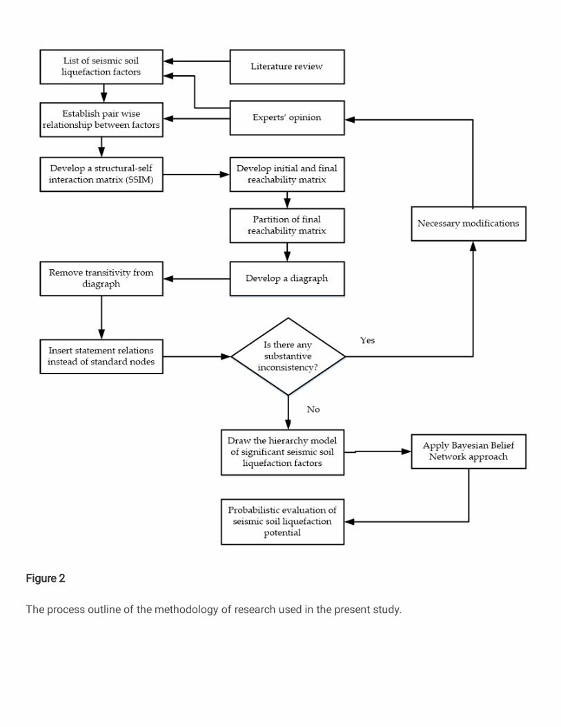
Figure 2

The process outline of the methodology of research used in the present study.

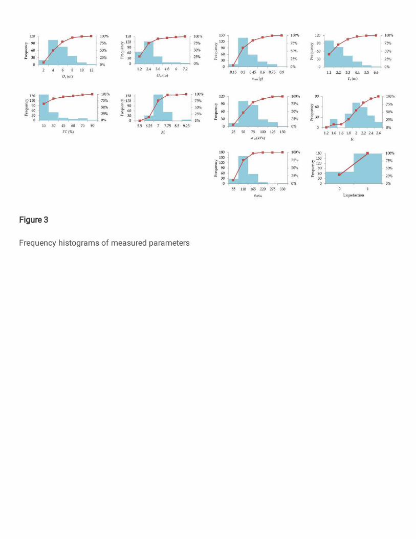
Figure 3

Frequency histograms of measured parameters

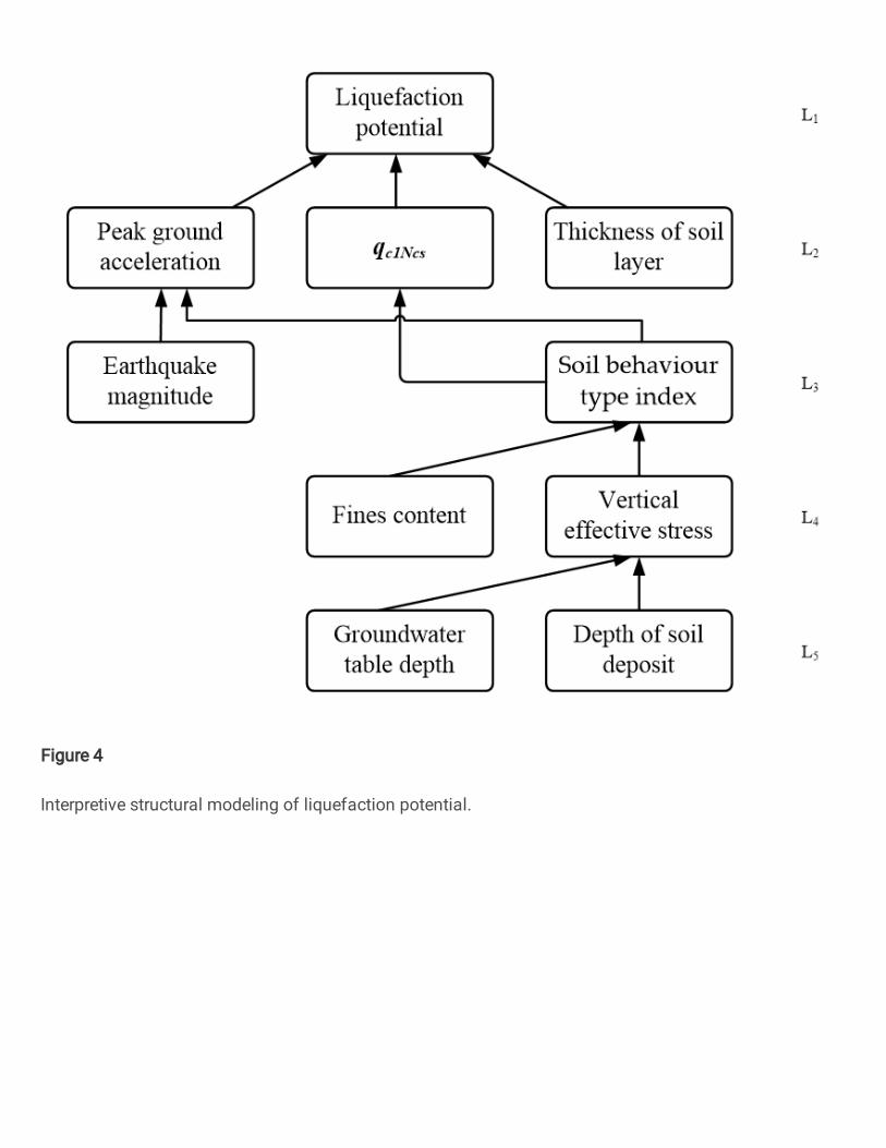
Figure 4

Interpretive structural modeling of liquefaction potential.

Figure 5

Liquefaction potential graphical model.

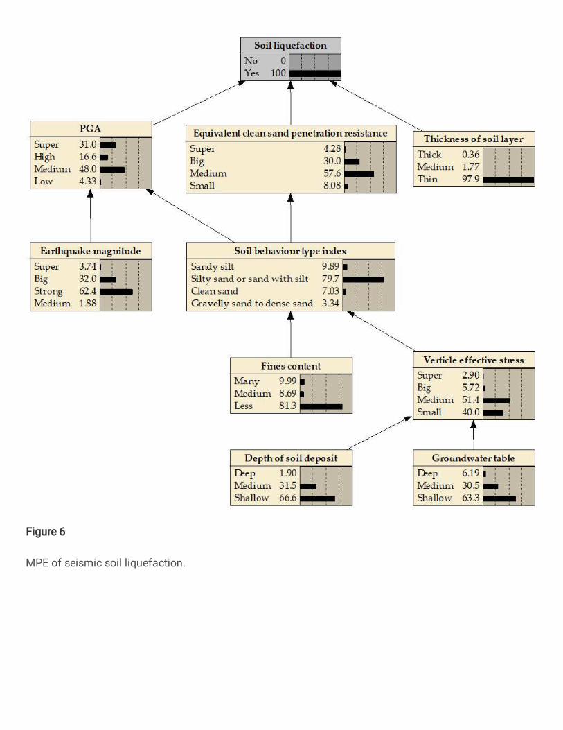
Figure 6

MPE of seismic soil liquefaction.

Documents

Probabilistic Evaluation of CPT-based Seismic Soil