Probabilistic Graphical Models - Computer ScienceProbabilistic Graphical Models COMP 790COMP 790-90 Seminar90 Seminar Spring 2011 The UNIVERSITY of NORTH CAROLINA at CHAPEL HILL Outline

Probabilistic Graphical ModelsProbabilistic Graphical Models

COMP 790 90 SeminarCOMP 790-90 Seminar

Spring 2011

The UNIVERSITY of NORTH CAROLINA at CHAPEL HILL

OutlineOutline

I t d tiIntroductionRepresentationBayesian networkBayesian network

Conditional IndependenceInference: Variable elimination LearningLearning

Markov Random FieldCliqueP i i MRFPair-wise MRF

Inference: Belief Propagation

Conclusion

COMP 790-090 Data Mining: Concepts, Algorithms, and Applications2

IntroductionIntroduction

Graphical Model:

+Probability Theory Graph Theory

Probability theory: ensures consistency, provides interface models to dataprovides interface models to data.

Graph theory: intuitively appealing interface for humans, efficient general purpose algorithms.


, g p p g


Modularity: a complex system is built by combining simpler partscombining simpler parts.

Provides a natural tool for two problems:

Uncertainty and ComplexityPlays an important role in the design and y p ganalysis of machine learning algorithms



Many of the classical multivariate probabilistic systems are special cases of the general graphical model formalism:

Mixture modelsu e ode sFactor analysisHidden Markov ModelsKalman filters

The graphical model framework provides a way to view all of these systems as instances of common underlying formalism.

Techniques that have been developed in one field can be transferred h fi ldto other fields

A framework for the design of new system


RepresentationRepresentation

A graphical model represent probabilistic relationships between a set of random variables.Variables are represented by nodes:

Binary events, Discrete variables, Continuous variables

Conditional (in)dependency is t d b ( b f) drepresented by (absence of) edges.

Directed Graphical Model: (Bayesian network)Undirected Graphical Model: (Markov Random Field)


OutlineOutline

IntroductionRepresentationBayesian networkBayesian network

Conditional IndependenceInference: Variable elimination LearningLearning

Markov Random FieldCliquePair-wise MRF


Conclusion


Bayesian NetworkBayesian Network

Directed acyclic graphs (DAG) ParentsDirected acyclic graphs (DAG).Directed edges give causality relationships between variables

Parents

pFor each variable X and parents pa(X) exists a conditional

b bilit P(X| (X))probability --P(X|pa(X))Discrete Variables: Conditional Probability Table(CPT)Probability Table(CPT)

Description of a noisy “causal” process


A Example: What Causes Grass Wet?


More Complex ExampleMore Complex Example

Diagnose the engine start problemDiagnose the engine start problem


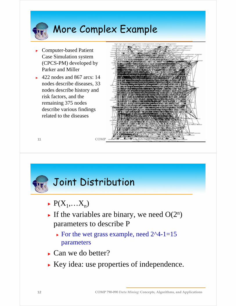
More Complex ExampleMore Complex Example

C b d iComputer-based Patient Case Simulation system (CPCS-PM) developed by Parker and Miller

422 nodes and 867 arcs: 14 nodes describe diseases, 33 ,nodes describe history and risk factors, and the remaining 375 nodes e a g 375 odesdescribe various findings related to the diseases


Joint DistributionJoint Distribution

P(X X )P(X1,…Xn)

If the variables are binary, we need O(2n)parameters to describe P

For the wet grass example, need 2^4-1=15 parameters

Can we do better?

Key idea: use properties of independence.


Independent Random VariablesIndependent Random Variables

X is independent of Y ifffor all values x,y)()|( xXPyYxXP y

If X and Y are independent then)()|( y

)()()()|()( YPXPYPYXPYXP

Unfortunately most of random variables of

)()()()|()( ,

)()...()()...( 21,1 nn XPXPXPXXP Unfortunately, most of random variables of interest are not independent of each other

The wet grass example


g p

Conditional IndependenceConditional IndependenceA more suitable notion is that of conditionalA more suitable notion is that of conditional independence.

X and Y are conditionally independent given ZX and Y are conditionally independent given Z

N i)|()|()|,(

)|(),|(

ZYPZXPZYXP

ZXPYZXP

Notation:

The conditionally independent structure in the )|,( ZYXI

Cgrass exampleI(S,R|C)

C

S R


I(C,W|S,R)W

Conditional IndependenceConditional Independence

Directed Markov Property:

Each random variable X, is Y1

Parent

conditionally independent of

its non-descendents, X

Y1

Y2D sc nd ntgiven its parents Pa(X)

Formally,

X

Y

Y2Descendent

y,P(X|NonDesc(X), Pa(X))=P(X|Pa(X))

Notation: I (X, NonDesc(X) | Pa(X))

Y3

Y Non descendent


Y4 Non-descendent

Factorized RepresentationFactorized RepresentationFull Joint distribution is defined in terms of local conditional distributions(obtained via the chain rule)

))(|(),,( 1 iin xpaxpxxP

Graphical Structure encodes conditional independences among random variables

))(|(),,( 1 iin pp

gRepresent the full joint distribution over the variables more compactly

Complexity reductionComplexity reductionJoint probability of n binary variables O(2n)Factorized form O(n*2k)


( )k: maximal number of parents of a node

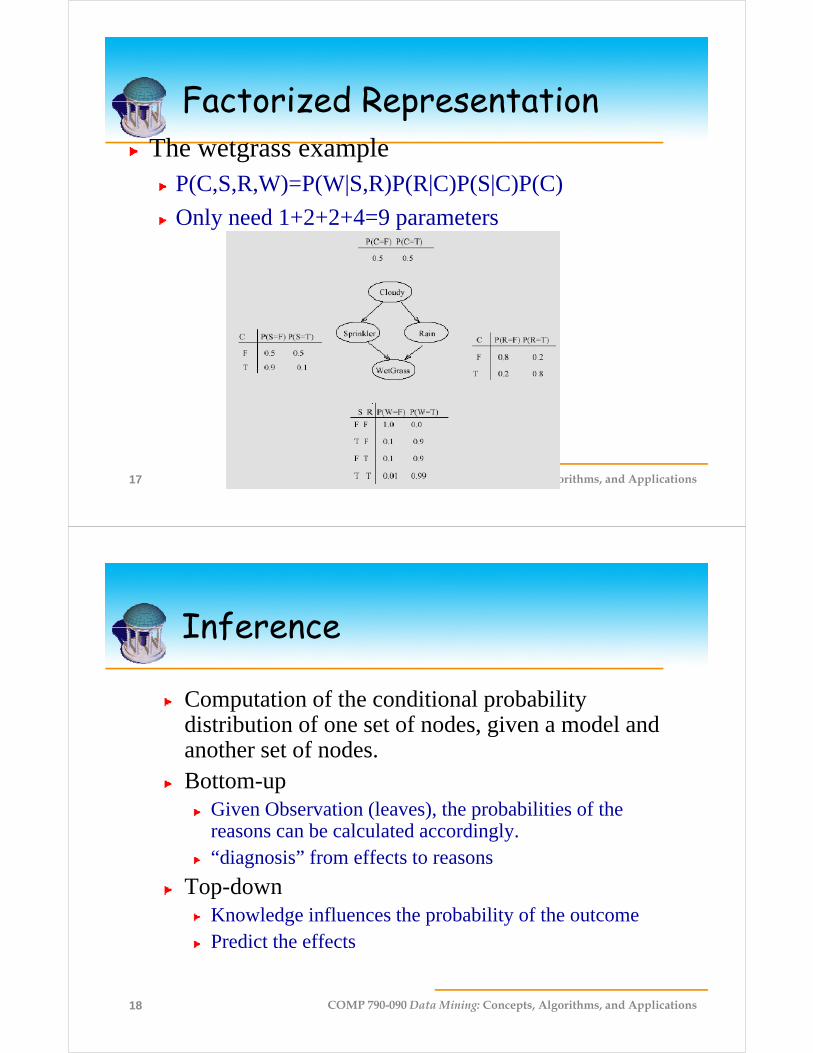
Factorized RepresentationFactorized RepresentationThe wetgrass example

P(C,S,R,W)=P(W|S,R)P(R|C)P(S|C)P(C)

Only need 1+2+2+4=9 parameters


InferenceInference

C i f h di i l b biliComputation of the conditional probability distribution of one set of nodes, given a model and another set of nodes.another set of nodes.Bottom-up

Given Observation (leaves), the probabilities of the reasons can be calculated accordingly.“diagnosis” from effects to reasons

Top downTop-downKnowledge influences the probability of the outcomePredict the effects


Basic ComputationBasic Computation

The value of x depends on yThe value of x depends on yDependency: conditional probability P(x|y)Knowledge about y: prior probability P(y)

yg y p p y (y)

Product rule)()|(),( yPyxPyxP

xSum rule (Marginalization)

y

yxPxP ),()( x

yxPyP ),()(

x

Bayesian ruley x

)()|()|(

yPyxPxyP prior likelihood lconditiona

poserior


)()|(

xPxyP

likelihoodposerior

Inference: Bottom UP Inference: Bottom UP Observe: wet grass (denoted by W=T)Observe: wet grass (denoted by W T)

Two possible causes: rain or sprinkle. Which is more likely?

Apply Bayes’ rule

)( TWP

0045.018.00495.00324.0009.00396.0

),,,(,,

rscTWrRsScCP

6471.0


Inference: Bottom UP Inference: Bottom UP

C S R W P( )

T T T T 0.99*0.8*0.1*0.5=0.0396

T T F T 0 9*0 2*0 1*0 5=0 009T T F T 0.9 0.2 0.1 0.5=0.009

T F T T 0.9*0.8*0.9*0.5=0.324

T F F T 0*0.2*0.9*0.5=0

F T T T 0.99*0.2*0.5*0.5=0.0495

F T F T 0.9*9.8*0.5*0.5=0.18

F F T T 0.9*0.2*0.5*0.5=0.045


F F F T 0*0.8*0.5*0.5=0



Apply Bayes’ rule

),(

)|(

TWTSP

TWTSP

),,,(

)(

,

TWrRTScCP

TWP

rc

43.064710

2781.0

64710

18.00495.0009.00396.0

)(

TWP


6471.06471.0



Apply Bayes’ rule

),(

)|(

TWTRP

TWTRP

),,,(

)(

,

TWTRsScCP

TWP

sc

708.064710

4581.0

64710

045.00495.0324.00396.0

)(

TWP


6471.06471.0

Inference: Top-downInference: Top-down

Th b bilit th t th ill b tThe probability that the grass will be wet given that it is cloudy.

WRS

RS

WRSCP

WRSCP

TCP

TCTWPTCTWP ,

),,,(

),,,(

)(

),()|(

WRS ,,),,,()(

C

S R


W

Inference AlgorithmsInference Algorithms

Exact inference problem in general graphical model is NP-hardExact Inference

Variable eliminationM i l ithMessage passing algorithmClustering and joint tree approach

Approximate InferenceApproximate InferenceLoopy belief propagationSampling (Monte Carlo) methods


Variational methods

Variable EliminationVariable Elimination

Computing P(W=T)Computing P(W T)Approach 1. Blind approach

Sum out all un-instantiated variables from the full jointj

Computation Cost O(2n)Th t lThe wetgrass example

Number of additions: 14Number of products:?


Solution: explore the graph structure

Variable Elimination

Approach 2: Interleave sums and Products

Variable Elimination

Approach 2: Interleave sums and ProductsThe key idea is to push sums in as far as possible

iIn computationFirst compute:Then compute:And so on

Computation Cost O(n*2k)For wetgrass example


For wetgrass exampleNumber of Additions:?Number of products:?

LearningLearning


LearningLearning

Learn parameters or structure from dataStructure learning: find correct connectivityStructure learning: find correct connectivity between existing nodesParameter learning: find maximumParameter learning: find maximum likelihood estimates of parameters of each conditional probability distributionp yA lot of knowledge (structures and probabilities) came from domain experts


p ) p

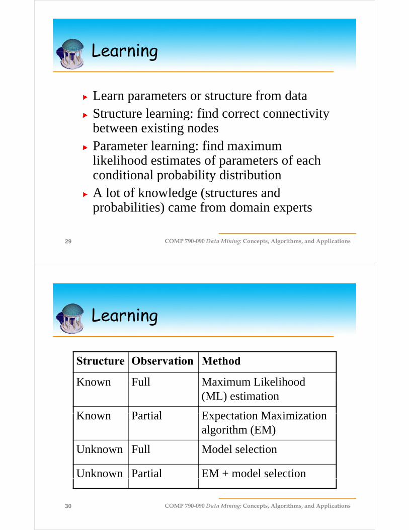
LearningLearning

Structure Observation Method

Known Full Maximum LikelihoodKnown Full Maximum Likelihood (ML) estimation

K P ti l E t ti M i i tiKnown Partial Expectation Maximization algorithm (EM)

U k F ll M d l l iUnknown Full Model selection

Unknown Partial EM + model selection


Model Selection MethodModel Selection Method

Select a 'good' model from all possible models and use it as if it were the correct model

Having defined a scoring function, a search algorithm is then used to find a network structure that receives the highest score fitting the prior kno ledge and datahighest score fitting the prior knowledge and data

Unfortunately, the number of DAG's on n variables is super-exponential in n. The usual approach is therefore p p ppto use local search algorithms (e.g., greedy hill climbing) to search through the space of graphs.


EM AlgorithmEM Algorithm

Expectation (E) stepUse current parameters to estimate the unobservedUse current parameters to estimate the unobserved data

Maximization (M) stepMaximization (M) stepUse estimated data to do ML/MAP estimation of the parameterthe parameter

Repeat EM steps, until convergence


OutlineOutline

I t d tiIntroductionRepresentationBayesian networkBayesian network

Conditional IndependenceInference LearningLearning

Markov Random FieldCliqueP i i MRFPair-wise MRF


Conclusion


Markov Random FieldsMarkov Random FieldsUndirected edges simply give correlations between g p y gvariables

The joint distribution is product of local functions over the cliques of the graph

CC xPZ

xP )(1

)(

where are the clique potentials, and Z is a normalization constant

CZ)( CC xP

w

zy

xw

zy

x

),,(),,(1

),,,( zyxPwyxPZ

wzyxP BA


w

zy

x

Z

The Clique The Clique

A liA cliqueA set of variables which are the arguments of a l l f tilocal function

The order of a cliqueThe number of variables in the clique

Example:p),()(),()()(),...,( 534,332,12151 xxPxxPxxxPxPxPxxP EDCBA


first order clique third order clique second order clique

Regular and Arbitrary GraphRegular and Arbitrary Graph


Pair-wise MRFPair-wise MRF

The order of cliques is at most twoThe order of cliques is at most two.

Commonly used in computer vision applications.Infer underline unknown variables through local observation andInfer underline unknown variables through local observation and the smooth prior

o1 o2 o3Observed image

φ2(i2) φ3(i3)φ1(i1)

o4 o5 o6

i1 i2 i3Underlying truth

φ5(i5)(i2,

i 5)

φ6(i6)φ4(i4)

ψ12(i1, i2) ψ23(i2, i3)

(i3,

i 6)

(i1,

i 4)

o7 o8 o9

i4 i5 i6ψ45(i4, i5)

φ5(i5)

ψ56(i5, i6)

ψ25

i 5, i

8)

φ6(i6)φ4(i4)

i 6, i

9)ψ

36

i 4, i

7)ψ

14

compatibility


o7 o8 o9

i7 i8 i9

ψ58

(i φ8(i8)φ7(i7) φ9(i9)

ψ78(i7, i8) ψ89(i8, i9)

ψ69

(i

ψ47

(i

Pair-wise MRFo1 o2 o3

Observed imageφ (i ) φ (i )φ (i )

Pair-wise MRF1 2 3

o4 o5 o6


2, i 5

)

φ2(i2) φ3(i3)φ1(i1)

ψ12(i1, i2) ψ23(i2, i3)

3, i 6

)

1, i 4

)

o4 o5 o6

i4 i5 i6

ψ45(i4, i5)

φ5(i5)

ψ56(i5, i6)

ψ25

(i2

i 8)

φ6(i6)φ4(i4)

i 9)

ψ36

(i3

i 7)

ψ14

(i1

(i i ) i * t i

o7 o8 o9

i7 i8 i9

ψ58

(i5,

φ8(i8)φ7(i7) φ9(i9)

ψ78(i7, i8) ψ89(i8, i9)

ψ69

(i6,

ψ47

(i4,

ψxy(ix, iy) is an nx * ny matrix.

φx(ix) is a vector of length nx, where nx is the number of states of ix.


Pair-wise MRFo1 o2 o3


Pair-wise MRF1 2 3

o4 o5 o6


2, i 5

)

φ2(i2) φ3(i3)φ1(i1)

ψ12(i1, i2) ψ23(i2, i3)

3, i 6

)

1, i 4

)

o4 o5 o6

i4 i5 i6

ψ45(i4, i5)

φ5(i5)

ψ56(i5, i6)

ψ25

(i2

i 8)

φ6(i6)φ4(i4)

i 9)

ψ36

(i3

i 7)

ψ14

(i1

Gi ll th id d t t fi d th t lik l t t f

o7 o8 o9

i7 i8 i9

ψ58

(i5,

φ8(i8)φ7(i7) φ9(i9)

ψ78(i7, i8) ψ89(i8, i9)

ψ69

(i6,

ψ47

(i4,

Given all the evidence nodes yi, we want to find the most likely state for all the hidden nodes xi, which is equivalent to maximizing

iijiij xxxZ

xP )(),(1

})({


ij i

iijiijZ)()(})({

Belief Propagationo1 o2 o3


Belief Propagation1 2 3

o4 o5 o6


2, i 5

)

φ2(i2) φ3(i3)φ1(i1)

ψ12(i1, i2) ψ23(i2, i3)

3, i 6

)

1, i 4

)

o4 o5 o6

i4 i5 i6

ψ45(i4, i5)

φ5(i5)

ψ56(i5, i6)

ψ25

(i2

i 8)

φ6(i6)φ4(i4)

i 9)

ψ36

(i3

i 7)

ψ14

(i1

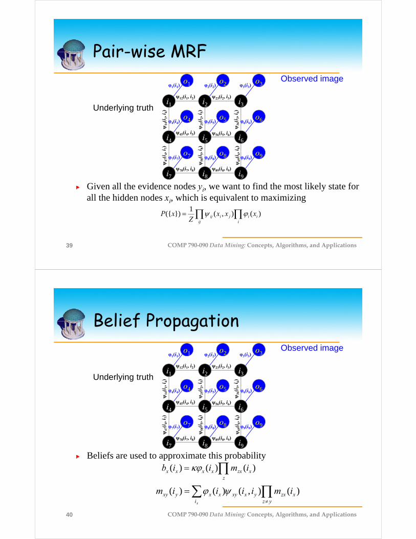
B li f d t i t thi b bilit

o7 o8 o9

i7 i8 i9

ψ58

(i5,

φ8(i8)φ7(i7) φ9(i9)

ψ78(i7, i8) ψ89(i8, i9)

ψ69

(i6,

ψ47

(i4,

Beliefs are used to approximate this probability

z

xzxxxxx imiib )()()(


xi yz

xzxyxxyxxyxy imiiiim )(),()()(

Belief Propagation

i

Belief Propagation

o5

i2

φ5(i5)m2-

>5(

i 5)

i4 i5 i6

φ5( 5)

m4->5(i5) m6->5(i5)

m

5(x 5

)

5(i 5

)

i8

m8-

>5

m8-

>5

Beliefs are used to approximate this probability)()()()()()( 5855655455255555 imimimimiib


Belief PropagationBelief Propagation

i2

i 5) (i5)

i1

i 4)

o5

x4 i5 i6

ψ45(i4, i5)φ5(i5)

ψ56(i5, i6)

ψ25

(i2,

8)

m45(i5) m65(i5)

m25

)

o4

i4

φ4(i4)

4)m

14(i

i8

ψ58

(i5,

i 8

65 5

m85

(i5)

i7

m74

(i4

Beliefs are used to approximate this probability)()()()()()( 5855655455255555 imimimimiib


4

)()(),()()( 474414544544545i

imimiiiim

Belief Propagation

φ(i ) and ψ (i i )

Belief Propagation

F d

φ(ix) and ψxy(ix,iy)

For every node ix

Compute m (i )

N

Compute mzx(ix)for each neighbor iz

Does bx(ix) converge?Y

Compute bx(ix)Output most likely

state for every node i


state for every node ix

Application: Learning Based Image Super Resolution

Extrapolate higher resolution images from low-p g gresolution inputs.

The basic assumption: there are correlations between low frequency and high frequency information.

A node corresponds to an image patchφx(xp): the probability of high frequency given observed low frequency

ψxy(xp, xq): the smooth prior between neighbor patches


Image Super ResolutionImage Super Resolution

(a) Images from a "generic" example set.

(b) Input (magnified x4) (c) Cubic spline (d) Super-resolution result (e) Actual full-resolution


ConclusionConclusion

A graphical representation of the probabilistic structure of a set of random variables, along with f ti th t b d t d i th j i tfunctions that can be used to derive the joint probability distribution.

I t iti i t f f d liIntuitive interface for modeling.

Modular: Useful tool for managing complexity.

C f li f d lCommon formalism for many models.


ReferencesReferences

K i M h I t d ti t G hi l M d l T h i lKevin Murphy, Introduction to Graphical Models, Technical Report, May 2001.M. I. Jordan, Learning in Graphical Models, MIT Press, 1999.Yijuan Lu, Introduction to Graphical Models, http:// www.cs.utsa.edu/~danlo/teaching/cs7123/Fall2005/Lyijuan.www.cs.utsa.edu/ danlo/teaching/cs7123/Fall2005/Lyijuan.ppt.Milos Hauskrecht, Probabilistic graphical models, http://www cs pitt edu/~milos/courses/cs3710/Lectures/Clashttp://www.cs.pitt.edu/~milos/courses/cs3710/Lectures/Class3.pdf.P. Smyth, Belief networks, hidden Markov models, and M k d fi ld if i i P tt R iti


Markov random fields: a unifying view, Pattern Recognition Letters, 1998.

ReferencesReferences

F R Kschischang B J Frey and H A Loeliger 2001F. R. Kschischang, B. J. Frey and H. A. Loeliger, 2001. Factor graphs and the sum-product algorithm IEEE Transactions on Information Theory, February, 2001.Y didi J S F W T d W i Y U d t diYedidia J.S., Freeman W.T. and Weiss Y, Understanding Belief Propagation and Its Generalizations, IJCAI 2001 Distinguished Lecture track. William T. Freeman, Thouis R. Jones, and Egon C. Pasztor, Example-based super-resolution, IEEE Computer Graphics and Applications, March/April, 2002.p pp pW. T. Freeman, E. C. Pasztor, O. T. Carmichael Learning Low-Level Vision International Journal of Computer Vision, 40(1), pp. 25-47, 2000.


Vision, 40(1), pp. 25 47, 2000.

Documents

Probabilistic Graphical Models - Computer ScienceProbabilistic Graphical Models COMP 790COMP 790-90 Seminar90 Seminar Spring 2011 The UNIVERSITY of NORTH CAROLINA at CHAPEL HILL Outline