1

Abstract—Reliable data delivery in the Internet of Things (IoT)

is very important in order to provide IoT-based services with the

required quality. However, IoT data delivery may not be

successful for different reasons, such as connection errors,

external attacks, or sensing errors. This results in data

incompleteness, which decreases the performance of IoT

applications. In particular, the recovery of missing data among the

massive sensed data of the IoT is so important that it should be

solved. In this paper, we propose a probabilistic method to recover

missing (incomplete) data from IoT sensors by utilizing data from

related sensors. The main idea of the proposed method is to

perform probabilistic matrix factorization (PMF) within the

preliminary assigned group of sensors. Unlike previous PMF

approaches, the proposed model measures the similarity in data

among neighboring sensors and splits them into different clusters

with a K-means algorithm. Simulation results show that the

proposed PMF model with clustering outperforms support vector

machine (SVM) and deep neural network (DNN) algorithms in

terms of accuracy and root mean square error. By using

normalized datasets, PMF shows faster execution time than SVM,

and almost the same execution time as the DNN method. This

proposed incomplete data–recovery approach is a promising

alternative to traditional DNN and SVM methods for IoT

telemetry applications.

Index Terms: Internet of Things (IoT), recovery of missing

sensor data, probabilistic matrix factorization, massive sensed

data

I. INTRODUCTION

UE to advancements in information technology, the

Internet of Things (IoT) has been emerging as the next big

thing in our daily lives. It is defined as a global network with an

infrastructure that has self-configuring capabilities [1]. The IoT

is an intelligent network that connects billions of things via the

Manuscript received March 23, 2017. This research was supported by a

Korea University grant.

Berihun Fekade is with Korea University, Sejong Metropolitan City, S.

Korea, and the Eindhoven University of Technology, Eindhoven, Netherlands

(e-mail: berihunfekade@gmail.com).

Taras Maksymyuk is with Department of Telecommunications, Lviv

Polytechnic National University, Lviv, Ukraine (e-mail:

taras.maksymyuk.ua@ieee.org).

Maryan Kyryk is with Department of Telecommunications, Lviv

Polytechnic National University, Lviv, Ukraine, (e-mail: mkyryk@gmail.com).

Minho Jo (Corresponding Author) is with Department of Computer

Convergence Software, Korea University, Sejong Metro City, S. Korea (phone:

+82-44-860-1348; fax: +82-44-860-1584; e-mail: minhojo@korea.ac.kr).

Internet by using a variety of communications technologies,

such as conventional Long Term Evolution (LTE), Wi-Fi,

ZigBee, wireless sensor networks (WSNs), Ethernet, as well as

specially developed Internet Protocol Version 6 (IPv6) over

low-power wireless personal area networks (6LoWPAN), the

low-power wide area network from the LoRa Alliance

(LoRaWAN), LTE machine type communications (LTE-MTC),

narrowband IoT (NB-IoT), and many other communications

technologies. Therefore, the IoT is rapidly transforming into a

highly heterogeneous ecosystem that provides interoperability

among different types of devices and communications

technologies.

The IoT achieves the goal of intelligent identification,

location, tracking, monitoring, and managing of things [2]. It

also creates additional value for a better life by sharing the

information collected among different things, and it integrates

and consolidates services at the edge using different IoT

gateways. IoT implementation requires new solutions to

integrate different physical objects (things) into a global IoT

ecosystem so that all of them can be identified and recognized

automatically. To achieve this, we need a reliable transmission

medium to communicate among things, and an intelligent

processing tool, such as cloud or fog computing, to generate

additional value from IoT applications.

According to recent analytics, we expect more than

100 billion IoT devices by 2025, whereas global financial

revenue from the IoT will grow from US$3.9 trillion to US$11.1

trillion [3, 4]. However, with its future implications, the IoT

brings substantial challenges, such as security, privacy, and

reliability, which need to be considered as well [5, 6].

IoT applications collect a huge amount of data from all

connected sensors. When some of the sensors do not send their

measured data to the cloud database, the performance of related

applications decreases. Missing data values affect the decision

making process for application servers that are used for a

specific task. The resulting errors can be significant for the next

steps in data processing. For example, in modern metropolitan

transportation systems, missing values will cause big problems

in determining the current locations of trains and buses. This

may cause many dangerous situations, especially in subway

systems, where any wrong decision could result in a collision.

Therefore, the missing values from sensors need to be recovered

to resolve such issues, and provide better data output based on

Probabilistic Recovery of

Incomplete IoT Sensed Data Berihun Fekade, Taras Maksymyuk, Member, IEEE, Maryan Kyryk, and Minho Jo, Senior Member,

IEEE

D

2

previous patterns or data from neighboring sensors.

In this paper, we propose a new approach to recovering

missing data in IoT outdoor and indoor telemetry systems. Our

approach implements a K-means clustering algorithm to

separate sensors into different groups. The main goal of

clustering is to ensure that sensors within one group will have

similar patterns of measurement. After clustering, we apply a

probabilistic matrix factorization (PMF) algorithm within each

cluster. Since the sensors are grouped according to similarity in

their measurements, it is possible to recover missing sensor data

by analyzing patterns of neighboring sensors. To improve the

performance of data recovery, we enhance the PMF algorithm

by normalizing the data and limiting the probabilistic

distribution of random feature matrices.

The rest of this paper is organized as follows. Section 2

discusses related work. Section 3 covers a detailed description

of the proposed method. Section 4 presents simulation results

and a performance analysis of the proposed method against

existing solutions. Section 5 concludes the research.

II. RELATED WORK

In the modern IoT paradigm, data integrity becomes the most

important aspect that influences the overall performance of any

system. The IoT is used for many critical applications, such as

telemetry in hazardous environments, control of industrial

processes, e-Health, smart transportation systems, national

security, etc. Each of these applications has strict requirements

for data integrity, correctness, and on-time delivery. However,

there are many issues that can cause problems with data in the

IoT. For example, data can be incomplete due to intrusion

attacks, connection errors, or problems with the measuring

sensors.

The problem of missing data from sensors has been widely

known in wireless sensor networks (WSNs) for a long time.

There are many solutions to recover missing data in WSNs, but

all of them require a direct connection between sensor nodes.

Li and Parker [7] proposed a spatial-temporal replacement

scheme to recover missing data by considering the nature of a

WSN. Their approach uses neighboring sensor readings if a

target node has no readings. Therefore, if the neighboring node

detects a change, it is very likely that there are some changes in

the environment.

Fig. 1. Sensor usage in the IoT infrastructure.

A similar approach was proposed by Gruenwald and

Halatchev [8], where the authors also recover missing values by

utilizing data from neighboring nodes. However, their approach

is more advanced, because they introduced a

window-association rule-mining algorithm to determine the

sensor node that is related to the sensor node with the missing

value. However, this approach determines the relation between

only two sensor nodes. In order to overcome this limitation, they

proposed a data estimation technique by using closed

itemset-based association rule mining that can determine the

relations between two or more sensors to recover missing values

[10].

In this paper, we focus mostly on a centralized IoT system

where each sensor is connected to the network independently,

and there are no direct connections between sensors. Fig. 1

illustrates the system model of the centralized IoT system. As

shown in Fig. 1, data from location 1 are missing due to a

connection problem, while data from sensors in location 2 are

sent without problem to the desired application servers. By

clustering sensors that have a minimal distance, it is possible to

3

recover missing sensor data from other sensors in the cluster. In

order to use an imputation scheme that utilizes time and space

information, several algorithms for estimating missing sensor

data have been proposed so far.

The simplest method is mean substitution, which imputes the

average value of all non-missing values to replace the missing

value. However, mean substitution does not preserve the

relation between variables, and thus, does not provide correct

estimations in most cases [15]. Other promising approaches for

prediction are the deep neural network (DNN) [17], and the

support vector machine (SVM) [18]. Both of these approaches

show excellent results in recommendation systems while

solving classification tasks. However, their application to our

task of missing-data recovery meets a number of problems. The

main problem in both DNNs and SVMs is that they classify a set

of data into different groups. Then, missing data are recovered

by estimating the corresponding group where missing values

may belong. Thus, the error between the predicted value and the

actual value is quite large, because the estimated value is

rounded to the nearest group.

Much more feasible for the current problem is the

probabilistic matrix factorization method. PMF is a Bayesian

probabilistic approach to factoring a big matrix into two

matrices. PMF has been proven to give good results in

recommendation systems, with an error 7% lower than that of

the Netflix movie recommendation system [19, 20]. However,

there are still some remaining challenges when applying PMF to

the missing data–recovery problem. First, the complexity

increases exponentially with increases in the matrix size.

Second, the overfitting problem may occur when the algorithm

is trying to minimize an error that results in a loss of generality.

In this paper, we overcome these drawbacks with PMF

algorithms by using preliminary clustering data normalization

and matrix regularization.

III. PROPOSED METHOD

A. Clustering sensors with a K-means algorithm

Considering the huge amounts of data collected in IoT

systems, it may be tricky to recover missing values in big data

arrays. Due to the nature of an IoT monitoring system, there is

always some degree of similarity among measured values of

neighboring sensors. Therefore, we first divide the sensors into

different groups to minimize the variation in measured values

within these groups. In our model, we use a K-means clustering

algorithm, which gives a good grouping for rectangular and

rounded areas. K-means is an unsupervised clustering algorithm

that divides a set of points into K clusters, so that the points in

each cluster tend to be near each other [16]. In our experiment,

all sensors are located in a room inside a building. Therefore, it

is convenient to apply a K-means algorithm to cluster

neighboring sensors.

Step 1. Define 1 2, ,..., NX x x x as a set of N sensor

locations that need to be clustered, and 1 2, ,..., KC c c c as a

set of K target cluster centers. Then, place cluster centers M

uniformly within the target field of sensors X.

Step 2. Associate each sensor in X to the nearest cluster

center (centroid) from set C by using criteria of the shortest

distance: 2

1

arg min , 1, ,k

i k

k K

Cx c i NX

(1)

1 2, ,..., , 1, , kC

n kX x x x n N C C

Step 3. For each cluster kC

X obtained from (1), compute the

cluster mean as follows:

1 , 1, , .

n

i

i

k

x

m k Kn

(2)

Step 4. Assign new locations of cluster centers C according

to the new values calculated in (2):

1 1 2 2, ,..., K KC C c m c m c m (3)

Step 5. Check the difference between new and previous

locations of cluster centers:

1

K

i i

i

C C C m c

(4)

Step 6. Iterate steps 2, 3, 4, and 5 until the following

condition is satisfied:

0C (5)

Condition (5) is a convergence criterion that indicates

clustering is complete, because further iterations will not change

current sensor groups kC

X .

Figure 2 describes the procedure in one iteration of steps 1

to 5. Different colors for the sensor points indicate membership

in different clusters.

4

kc

ix

i kx m

km

(a) (b) (c)

Fig. 2. Iteration of K-means clustering algorithm: a – step 1, b – steps 2 and 3, c – steps 4 and 5. .

B. Probabilistic matrix factorization to recover the missing

data in each cluster

In general, PMF is used to decompose a single matrix into a

product of two matrices. Application of PMF to the IoT has two

main advantages. First, PMF allows us to decrease the total

number of stored values for big-data arrays due to the lower

dimensionality of the resulting matrices after factorization. This

advantage is achieved only if the original matrix has large

dimensions. For small matrices, PMF may result in an even

higher number of values after factorization. The second

advantage with PMF is introduced in this paper. Since PMF has

a property to obtain the original matrix by computing a product

of two matrices, we can also use this property to recover missing

values in the original matrix. In this paper, we apply the

probabilistic matrix factorization model to recover the missed

data points for each cluster. The PMF process for missing-data

recovery is described below.

Step 1. Represent the original dataset as matrix R with

dimensions [NxM]:

11 1

1

M

N NM

R R

R R

R (6)

Step 2. Generate random U [NxK] and V [KxM] matrices, so

that:

11 1

T

1

M

N NM

R R

R R

R U V (7)

It is important that matrices (6) and (7) have exactly the same

dimensions in order to ensure correct output from missing data

recovery. K represents the number of latent feature

column-vectors in U and V, which determines the flexibility of

the PMF process. Note that K can be any integer, because it does

not have any impact on the resulting dimensions of matrix R.

However, it does have an impact on PMF performance, which

will be studied further in this paper.

Step 3. Define the missing data points as identity matrix I,

which has the same dimensions [NxM] as original matrix R:

11 1

1

M

N NM

I I

I I

I

Values in I are defined according to the following rule:

1, if is a known value

0, if is a missing value

ij

ij

ij

RI

R

Step 4. Calculate the root mean square error (RMSE)

between original matrix R and recovered matrix R:

2

1 1

N MT

ij ij i j

i j

RMSE I R U V

(8)

Step 5. Compare the RMSE value calculated in (8) with

maximum acceptable error RMSEmax:

maxRMSE RMSE (9)

If condition (9) is satisfied, the PMF algorithm is complete.

Otherwise, proceed to Step 6.

Step 6. Update the values of U and V as follows:

ij

i i

i

ij

j j

j

RMSEU U

U

RMSEV V

V

(10)

where the α – slope value defines how much the values in U and

V need to be adjusted. Steps 4, 5, and 6 are iterated until

condition (9) is satisfied. Note, that the correct value of α is very

important in order to achieve a good tradeoff between precision

and convergence time. Too large a value for α may result in low

precision, because RMSE will jump around the target point

RMSEmax. On the other hand, too small a value for α will result

in a many unnecessary iterations before RMSE approaches the

value that satisfies condition (9). Fig. 3 shows a comparison of

PMF performance for different values of α.

5

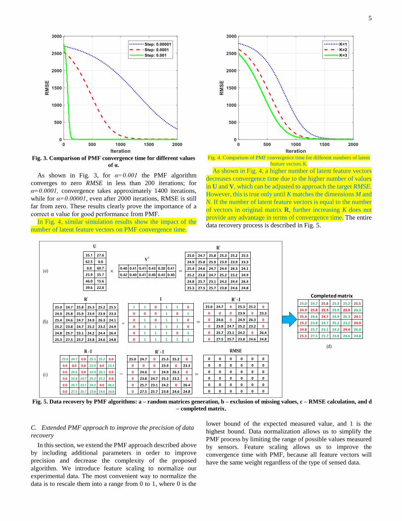
Fig. 3. Comparison of PMF convergence time for different values

of α.

As shown in Fig. 3, for α=0.001 the PMF algorithm

converges to zero RMSE in less than 200 iterations; for

α=0.0001, convergence takes approximately 1400 iterations,

while for α=0.00001, even after 2000 iterations, RMSE is still

far from zero. These results clearly prove the importance of a

correct α value for good performance from PMF.

In Fig. 4, similar simulation results show the impact of the

number of latent feature vectors on PMF convergence time.

Fig. 4. Comparison of PMF convergence time for different numbers of latent

feature vectors K.

As shown in Fig. 4, a higher number of latent feature vectors

decreases convergence time due to the higher number of values

in U and V, which can be adjusted to approach the target RMSE.

However, this is true only until K matches the dimensions M and

N. If the number of latent feature vectors is equal to the number

of vectors in original matrix R, further increasing K does not

provide any advantage in terms of convergence time. The entire

data recovery process is described in Fig. 5.

35.1 27.6

62.5 0.0

0.0 60.7

25.9 35.7

46.0 15.6

39.6 22.8

0.40 0.41 0.41 0.43 0.38 0.41

0.42 0.40 0.41 0.40 0.43 0.40

TV

U

25.0 24.7 25.8 25.3 25.2 25.5

24.9 25.8 25.9 23.9 23.9 23.3

25.4 24.6 24.7 24.9 26.3 24.1

25.2 23.8 24.7 25.2 23.2 24.9

24.8 25.7 23.1 24.2 24.4 26.4

25.3 27.5 25.7 23.8 24.6 24.8

R

25.0 24.7 25.8 25.3 25.2 25.5

24.9 25.8 25.9 23.9 23.9 23.3

25.4 24.6 24.7 24.9 26.3 24.1

25.2 23.8 24.7 25.2 23.2 24.9

24.8 25.7 23.1 24.2 24.4 26.4

25.3 27.5 25.7 23.8 24.6 24.8

R

1 1 0 1 1 0

0 0 0 1 0 1

0 1 0 1 1 0

0 1 1 1 1 0

0 1 1 1 0 1

0 1 1 1 1 1

I

25.0 24.7 0 25.3 25.2 0

0 0 0 23.9 0 23.3

0 24.6 0 24.9 26.3 0

0 23.8 24.7 25.2 23.2 0

0 25.7 23.1 24.2 0 26.4

0 27.5 25.7 23.8 24.6 24.8

R I

25.0 24.7 0.0 25.3 25.2 0.0

0.0 0.0 0.0 23.9 0.0 23.3

0.0 24.6 0.0 24.9 26.3 0.0

0.0 23.8 24.7 25.2 23.2 0.0

0.0 25.7 23.1 24.2 0.0 26.4

0.0 27.5 25.7 23.8 24.6 24.8

25.0 24.7 0 25.3 25.2 0

0 0 0 23.9 0 23.3

0 24.6 0 24.9 26.3 0

0 23.8 24.7 25.2 23.2 0

0 25.7 23.1 24.2 0 26.4

0 27.5 25.7 23.8 24.6 24.8

0 0 0 0 0 0

0 0 0 0 0 0

0 0 0 0 0 0

0 0 0 0 0 0

0 0 0 0 0 0

0 0 0 0 0 0

R I R I RMSE

25.0 24.7 25.8 25.3 25.2 25.5

24.9 25.8 25.9 23.9 23.9 23.3

25.4 24.6 24.7 24.9 26.3 24.1

25.2 23.8 24.7 25.2 23.2 24.9

24.8 25.7 23.1 24.2 24.4 26.4

25.3 27.5 25.7 23.8 24.6 24.8

Completed matrix

( )a

(b)

(c)

(d)

Fig. 5. Data recovery by PMF algorithms: a – random matrices generation, b – exclusion of missing values, c – RMSE calculation, and d

– completed matrix.

C. Extended PMF approach to improve the precision of data

recovery

In this section, we extend the PMF approach described above

by including additional parameters in order to improve

precision and decrease the complexity of the proposed

algorithm. We introduce feature scaling to normalize our

experimental data. The most convenient way to normalize the

data is to rescale them into a range from 0 to 1, where 0 is the

lower bound of the expected measured value, and 1 is the

highest bound. Data normalization allows us to simplify the

PMF process by limiting the range of possible values measured

by sensors. Feature scaling allows us to improve the

convergence time with PMF, because all feature vectors will

have the same weight regardless of the type of sensed data.

6

After data normalization, we assume that data in matrix R

follow a Gaussian distribution with mean value μ and standard

deviation σ, which reflects the uncertainty of the estimations:

,N

Therefore, we place zero-mean Gaussian priors on U and V

feature vectors, i.e. each row of U and V is a multivariate

Gaussian with mean μ=0 and precision that is some multiple of

identity matrix I. Those multiples are σU for U and σV for V.

2 2

1

| | 0,N

U i U

i

P U N U I

(11)

2 2

1

| | 0,N

V i V

i

P V N V I

(12)

The priors in equations (11) and (12) ensure that latent

variables of U and V will not grow too far from 0. This prevents

overly strong values of U and V matrices. Without limitation of

the values in U and V, the convergence time with PMF will

increase from more iterations, and higher complexity is the

result.

Taking into account prior distributions in equations (11) and

(12), the conditional distribution over the observed sensor data

is represented as follows:

2 2

1 1

| , , | ,ij

N M IT

ij i j

i j

P R U V N R U V

(13)

In order to minimize the RMSE, we need to maximize the log

posterior in equation (13), i.e. to ensure that obtained

distribution of values U∙VT matches the prior distribution of

values in original matrix R. Note that missing elements do not

affect the prior and posterior distribution in equation (13),

because they are excluded by multiplication with identity matrix

I.

To improve the performance of PMF with sparse matrices,

we use matrix regularization to avoid the overfitting problem.

Overfitting means that the algorithms performs very well on the

training dataset due to the high precision of feature vectors U

and V. However, testing-dataset performance is much worse

due to the loss of generality. In other words, a recovered matrix

reflects known values very precisely, but missing data values

approach zero, because the training dataset has been multiplied

with identity matrix I. Therefore, by avoiding overfitting, we

make the proposed PMF approach better suited to the problem

of missing-data recovery due to a more generalized output.

To avoid data overfitting, we fix the variance parameters σ,

σU, and σV as constants, and reduce the optimization problem to

a least-squares matrix completion problem with quadratic

regularization:

22 2

1 1 1 1

2 2

1

2 2

1

min

min ,

subject to: | | 0, ,

| | 0, ,

,

,

, , ,

N M N MT

ij ij i j U V

i j i i

N

U i U

i

N

V i V

i

U

U

V

V

V U

RMSE

I R U V U V

P U N U I

P V N V I

const

(14)

where ||U|| and ||V|| are Frobenius norms defined as the square

roots of the sum of the absolute squares of matrix elements:

2

1 1

2

1 1

N K

ij

i j

M K

ij

i j

U U

V V

(15)

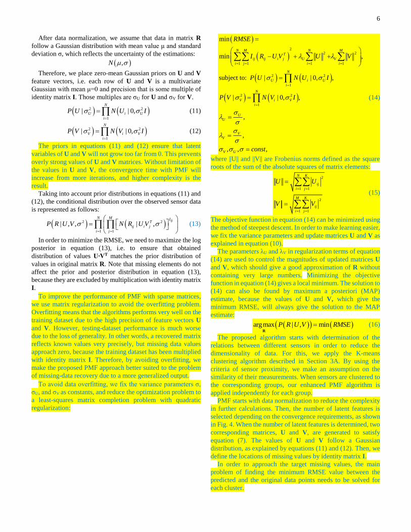
The objective function in equation (14) can be minimized using

the method of steepest descent. In order to make learning easier,

we fix the variance parameters and update matrices U and V as

explained in equation (10).

The parameters λU and λV in regularization terms of equation

(14) are used to control the magnitudes of updated matrices U

and V, which should give a good approximation of R without

containing very large numbers. Minimizing the objective

function in equation (14) gives a local minimum. The solution to

(14) can also be found by maximum a posteriori (MAP)

estimate, because the values of U and V, which give the

minimum RMSE, will always give the solution to the MAP

estimate:

argmax | , minP R U V RMSER

(16)

The proposed algorithm starts with determination of the

relations between different sensors in order to reduce the

dimensionality of data. For this, we apply the K-means

clustering algorithm described in Section 3A. By using the

criteria of sensor proximity, we make an assumption on the

similarity of their measurements. When sensors are clustered to

the corresponding groups, our enhanced PMF algorithm is

applied independently for each group.

PMF starts with data normalization to reduce the complexity

in further calculations. Then, the number of latent features is

selected depending on the convergence requirements, as shown

in Fig. 4. When the number of latent features is determined, two

corresponding matrices, U and V, are generated to satisfy

equation (7). The values of U and V follow a Gaussian

distribution, as explained by equations (11) and (12). Then, we

define the locations of missing values by identity matrix I.

In order to approach the target missing values, the main

problem of finding the minimum RMSE value between the

predicted and the original data points needs to be solved for

each cluster.

7

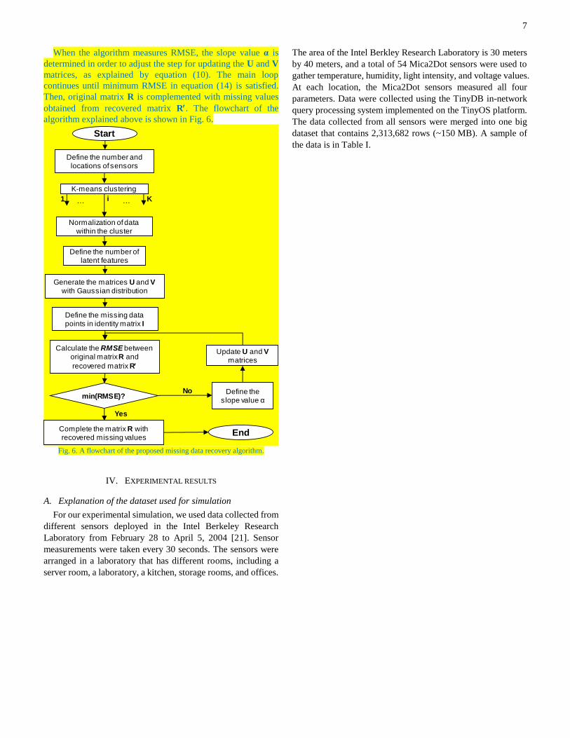
When the algorithm measures RMSE, the slope value α is

determined in order to adjust the step for updating the U and V

matrices, as explained by equation (10). The main loop

continues until minimum RMSE in equation (14) is satisfied.

Then, original matrix R is complemented with missing values

obtained from recovered matrix R. The flowchart of the

algorithm explained above is shown in Fig. 6.

Start

Define the number and locations of sensors

K-means clustering

… …1 Ki

Normalization of data within the cluster

Define the number of latent features

Generate the matrices U and Vwith Gaussian distribution

Define the missing data points in identity matrix I

Calculate the RMSE between original matrix R and

recovered matrix R

Complete the matrix R with recovered missing values

Update U and Vmatrices

min(RMSE)?Define the

slope value α

End

No

Yes

Fig. 6. A flowchart of the proposed missing data recovery algorithm.

IV. EXPERIMENTAL RESULTS

A. Explanation of the dataset used for simulation

For our experimental simulation, we used data collected from

different sensors deployed in the Intel Berkeley Research

Laboratory from February 28 to April 5, 2004 [21]. Sensor

measurements were taken every 30 seconds. The sensors were

arranged in a laboratory that has different rooms, including a

server room, a laboratory, a kitchen, storage rooms, and offices.

The area of the Intel Berkley Research Laboratory is 30 meters

by 40 meters, and a total of 54 Mica2Dot sensors were used to

gather temperature, humidity, light intensity, and voltage values.

At each location, the Mica2Dot sensors measured all four

parameters. Data were collected using the TinyDB in-network

query processing system implemented on the TinyOS platform.

The data collected from all sensors were merged into one big

dataset that contains 2,313,682 rows (~150 MB). A sample of

the data is in Table I.

8

Fig. 7. Sensor locations and clustering in the Intel Berkeley Research Laboratory.

Fig. 7 shows the locations of sensors and their clustering into

14 groups in the Intel Berkeley Research Laboratory. Sensors

within each cluster are enclosed by solid lines. PMF was applied

for data values of sensors within each cluster group. The main

reason for clustering the sensors is to find similarity between

their measurements that can be further exploited to find missing

sensor data. Fig. 8 shows temperature measurements from

sensors in two clusters. Here, sensors 25 and 26 are in the first

cluster (dashed and dash-dotted lines) and sensors 9 and 10 are

in a second cluster (solid and dotted lines). As observed in Fig. 8,

the measurements of sensors within one cluster follow very

similar patterns, whereas between clusters the difference is

much higher.

Thus, when there are missing values inside one cluster, we

can estimate them from neighboring nodes within the same

cluster group. In order to enhance the proposed approach, a

series of clusters was generated, starting from three groups and

increasing up to 20 groups.

For the given area in Fig. 7, the K-means algorithm was used

to generate a list of neighboring clustered sensors based on their

locations, i.e., the x and y coordinates relative to the upper right

corner of the lab. This approach allows the PMF algorithm to

work inside one cluster among closely related sensors. Other

sensors that are outside the cluster boundaries are not

considered under PMF. The prediction output of the PMF

model will improve as the number of cluster groups increases

(closer relations among sensors clustered into a single group).

The total number of sensors inside each cluster varied

depending on the generated list of sensors by using the K-means

clustering algorithm. The PMF algorithm was applied inside

each group. For example, in cluster 14, there are different, yet

closely related, sensors that are clustered together. These sensor

readings are organized to create a matrix that will be used for the

PMF model. Having k=20 clusters means that the area is

partitioned into 20 ideal groups of sensors.

TABLE I

DATA SAMPLE OBTAINED IN THE INTEL BERKELEY RESEARCH LABORATORY.

Date Time Sensor ID Temperature (C˚) Humidity (%) Light (Lux) Voltage (V)

2/28/2004 1:20:17 AM 49 17.4796 39.9929 121.44 2.66332

2/28/2004 1:22:46 AM 49 17.46 40.0268 121.44 2.67532

2/28/2004 1:11:46 AM 50 16.676 42.6516 79.12 2.66332

2/28/2004 1:12:17 AM 50 16.6956 42.5847 79.12 2.66332

2/28/2004 1:11:47 AM 51 17.7246 39.7896 136.16 2.67532

2/28/2004 1:12:17 AM 51 17.705 39.8235 136.16 2.67532

… … … … … … …

9

Fig. 8 Comparison of the measurements within and among

clusters.

B. Simulation parameters and results

First, we make 10% of the total data empty. The empty

dataset will be used to test the accuracy of the sensed data values,

compared to the original values. Using PMF, the latent vectors

are generated inside each selected cluster using the remaining

90% of the sensed data values as a training set. After getting the

latent vectors, it is possible to reconstruct the missing data and

complete the original matrix. Comparing the generated values

from the PMF with the original data gives insight into the

accuracy of the algorithm. We computed the difference between

the predicted values and the original values inside each cluster

to get the maximum error between them. The cluster that gives

the lowest RMSE, and also the lowest average difference

between the generated and original data, will be the optimal

solution. It is also clear that more dispersed sensor locations

within a group results in less accurate prediction of missing

values.

We compared the output of the recovered sensor data with

existing algorithms: a support vector machine with linear and

radial basis function (RBF) kernels, and a deep neural network

with two and three hidden layers. In order to adjust the recovery

problem to the SVM and the DNN, we altered the data

classification problem. Each data value was converted into a

discrete class value in the range from 0 to 1 with increments of

0.1. Thus, 11 classes were generated to fit normalized sensor

measurements into a classification problem (see Table II). After

discretizing the data, SVM and DNN algorithms used 90% of

the data as a training set and the remaining 10% as a test set for

algorithm accuracy.

Fifty-four sensors were clustered into different numbers of

groups starting between 3 and 20, and PMF output was

compared for all cases. Fig. 9 shows the simulation results for

the maximum prediction error in different numbers of clusters.

According to the obtained results, the maximum error decreases

by increasing the number of clusters. This result confirms the

theoretical expectations that a higher number of clusters will

increase accuracy owing to lower differences between the

measurements within smaller groups of sensors.

Fig. 9. Maximum prediction error of PMF for different numbers

of clusters.

Simulations were conducted by using Python 2.7.9 in the

PyCharm4 Community Edition development environment. The

“scikit-learn” package for Python has been used to solve the

classification problem by SVM and DNN methods [22]. For all

methods, we used 90% of the data as a training set, and 10% of

the data as a test set. Two implementations of SVM, with linear

and RBF kernels, were compared. DNN models with two and

three hidden layers were compared, with 100 nodes per hidden

layer. The learning rate of the DNN was set to 0.001. A rectified

linear unit function was used for activation of the DNN model.

Comparative-test results of the predicted sensor data values

and the original data values show that the data recovery

accuracy of the proposed method is very high, compared to the

SVM (linear & RBF kernels) and neural network methods. The

maximum error between actual and predicted values gradually

TABLE II

CLASS ASSIGNMENT FOR SVM AND DNN ALGORITHMS.

Class ID Data range

(normalized) Class

1 [0.00, 0.05] 0.0

2 (0.05, 0.15] 0.1

3 (0.15, 0.25] 0.2

4 (0.25, 0.35] 0.3

5 (0.35, 0.45] 0.4

6 (0.45, 0.55] 0.5

7 (0.55, 0.65] 0.6

8 (0.65, 0.75] 0.7

9 (0.75, 0.85] 0.8

10 (0.85, 0.95] 0.9

11 (0.95, 1.00] 1.0

10

decreases as the number of cluster groups increases, as shown in

Fig. 10. The PMF method enhances the complementarities

between sensors by imputing the most appropriate data values,

and it improves the reliability of the monitoring application.

Fig. 10. Comparison of RMSE for different models.

The accuracy of the PMF model compared to SVM and DNN

models is shown in Fig. 11. According to the obtained

simulation results, the PMF model outperforms both SVM and

DNN models. The reason for this huge gap in RMSE for both

SVM and DNN methods is that they are designed for

classification purposes, unlike the PMF method. Both SVM and

DNN methods predict the class numbers with a predefined step

of 0.1 that results in high inaccuracy. The PMF method can

operate with continuous data that give more accurate output.

The overall advantage of the PMF method over SVM and DNN

in terms of average RMSE is shown in Table III. A comparison

of the execution times for PMF, SVM, and DNN for both

training and testing datasets is shown in Table IV. The total size

of the dataset for execution is 5000 values. Results show that

PMF execution time is much faster than SVM and almost the

same as the DNN model.

Fig. 11. Comparison of accuracy for different models.

V. CONCLUSION

One of the problems in realizing the IoT is missing sensor

data values that are crucial for decision making processes in

different applications. The missing sensor values are necessary

for applications that require them as data input. By clustering

related sensors and using probabilistic matrix factorization, this

paper has shown how to recover massive amounts of missing

sensor data values. Our results show that by minimizing RMSE

using the PMF method inside a cluster of sensor nodes, missing

sensor values can be recovered more efficiently than with other

methods, such as SVM and DNN. The SVM and DNN methods

have less accuracy and higher RMSE values, compared to the

PMF method, due to loss of precision for continuous datasets.

The PMF model applied inside closely related sensors

shows better accuracy and lower RMSE results than other

methods. As the cluster size gets smaller (for better correlation

of measurements among sensors), accuracy also becomes better

compared to larger clusters. The reason is that a larger cluster

size contains more sensors, and the correlation between

measurements is not good among all sensors.

Results show that the PMF model gives more accurate and

realistic data for the imputation of missing sensor values. In

addition, the execution time of the PMF model is very close to

that of DNN, which makes the proposed approach very

promising for data recovery problems in the IoT.

In our future research, we will provide more insight into the

performance of the PMF algorithm in different scenarios.

Additional studies will be done on the sensor clustering problem,

since there are many parameters that need to be considered in

addition to the proximity of sensors. A flexible clustering

algorithm is needed to reflect the reasons for the missing data in

different sensors, and to find relations between sensors that are

more likely to fail in data measurements or communications

with the database.

TABLE IV

COMPARISON OF EXECUTION TIMES FOR PMF, SVM, AND DNN.

Model Name Training time, s Testing time, s

SVM (Linear Kernel) 18.265 0.190

SVM (RBF Kernel) 112.880 1.925

Deep Neural Network

(2 hidden layers) 0.204 0.003

Deep Neural Network

(3 hidden layers) 0.460 0.007

PMF 0.520 0.011

TABLE III

RMSE IMPROVEMENT WITH PMF OVER SVM AND DNN MODELS.

Id Model Name Average RMSE

Gap (%)

1 SVM (Linear Kernel) 79.30

2 SVM (RBF Kernel) 72.84

3

Deep Neural Network

(2 hidden layers) 67.50

4

Deep Neural Network

(3 hidden layers) 63.71

11

ACKNOWLEDGMENT

This research was supported by a Korea University grant.

REFERENCES

[1] Roberto Minerva, Abyi Biru, and Domenico Rotondi, “Towards a

definition of the Internet of Things (IoT)”, IEEE Internet Initiative, Torino,

Italy, 2015.

[2] Rose, Karen, Scott Eldridge, and Lyman Chapin, “The internet of things:

An overview”, The Internet Society (ISOC), October 2015.

[3] International Telecommunication Union, “Internet of Things Global

Standards Initiative”, June 2015,

http://handle.itu.int/11.1002/1000/11559.

[4] Huawei Technologies Co. Ltd., “Global Connectivity Index”, September

2015, http://www.huawei.com/minisite/gci/en/index.html.

[5] James Manyika, Michael Chui, Peter Bisson, Jonathan Woetzel, Richard

Dobbs, Jacques Bughin, and Dan Aharon, “The Internet of Things:

Mapping the Value Beyond the Hype”, McKinsey Global Institute, June

2015.

[6] Shanzhi Chen, Hui Xu, Dake Liu, Bo Hu and Hucheng Wang, “A vision

of IoT: Applications, challenges, and opportunities with china

perspective”, IEEE Internet of Things, Vol. 1, No 4, pp. 349-359, August

2014.

[7] YuanYuan Li and Lynne E. Parker, “A spatial‐temporal imputation

technique for classification with missing data in a wireless sensor

network”, IEEE International Conference on Intelligent Robots and

Systems, Nice, France, September 22-26, 2008.

[8] Le Gruenwald and Mihail Halatchev, “Estimating missing values in

related sensor data streams”, The 11th International Conference

Management of Data (COMADO5), pp. 83-94, 2005.

[9] David Williams, Xuejun Liao, Ya Xue and Lawrence Carin,

“Incomplete-Data Classification using Logistic Regression”, 22nd

International Conference on Machine Learning, Bonn, Germany, 2005.

[10] Nan Jiang and Le Gruenwald, “Estimating Missing Data in Data

Streams”, 12th International Conference on Database Systems for

Advanced Applications, Bangkok, Thailand, pp. 981-987, April 2007.

[11] Salakhutdinov, Ruslan, and Andriy Mnih, “Probabilistic matrix

factorization”, Neural Information Processing Systems, 2011.

[12] Andrea Kulakov and Danco Davcev, “Tracking of unusual events in

wireless sensor networks based on artificial neural-networks algorithms”,

IEEE International Conference on In Information Technology: Coding

and Computing, vol. 2, pp. 534-539, 2005.

[13] Gail A. Carpenter, Stephen Grossberg, and David B. Rosen, “Fuzzy ART:

Fast stable learning and categorization of analog patterns by an adaptive

resonance system”, Neural networks, vol. 4, no. 6, pp. 759-771, 1991.

[14] YuanYuan Li and Lynne E. Parker, “Detecting and monitoring

time-related abnormal events using a wireless sensor network and mobile

robot”, IEEE/RSJ International Conference on In Intelligent Robots and

Systems ( IROS ), pp. 3292-3298, 2008.

[15] Therese D. Pigott, “A Review of Methods for Dealing with Missing Data”,

Educational Research and Evaluation, Vol. 7, No. 4, pp. 353-383, 2000.

[16] James MacQueen, “Some methods for classification and analysis of

multivariate observations”, The fifth Berkeley symposium on

mathematical statistics and probability, Vol. 1, No. 14, pp. 281-297,

1967.

[17] Sung-Hwan Min, and Ingoo Han, "Recommender systems using support

vector machines", Springer Web Engineering, pp. 387-393, Berlin,

Heidelberg, 2005.

[18] Christina Christakou, Spyros Vrettos, and Andreas Stafylopatis, "A

hybrid movie recommender system based on neural networks",

International Journal on Artificial Intelligence Tools, Vol. 16, No. 05, pp.

771-792, October 2007.

[19] Ruslan Salakhutdinov, and Andriy Mnih, “Bayesian probabilistic matrix

factorization using MCMC”, 25th International Conference on Machine

Learning, Helsinki, Finland, 2008.

[20] Takács, Gábor, István Pilászy, Bottyán Németh, and Domonkos Tikk,

“Matrix factorization and neighbor based algorithms for the Netflix prize

problem”, the 2008 ACM conference on Recommender systems, pp.

267-274, 2008.

[21] http://db.csail.mit.edu/labdata/labdata.html

[22] http://scikit-learn.org/stable/modules/generated/sklearn.svm.SVC.html

Berihun Fekade is now a PDEng student with

Eindhoven University of Technology, Netherlands. He

received his MS degree in computer and information

science from Korea University, S. Korea in 2016, and

BA degree in electrical engineering from Arba Minch

University, Ethiopia in 2007. He has been working as

senior software engineer in "Cybersoft PLc", Addis

Ababa, Ethiopia from 2007 to 2013. His research

interests include mobile cloud computing, artificial

intelligence, probability theory in wireless

communications, and the Internet of Things (IoT)

Taras Maksymyuk (M’14) is now an Assistant

Professor of Telecommunications Department, Lviv

Polytechnic National University, Lviv, Ukraine. He did

his Post-doc Fellow course under Prof. Minho Jo and

was an invited Ph.D student in Korea Univ., Sejong, S.

Korea in 2017, 2015, respectively. He received his PhD

degree in telecommunication systems and networks in

2015, M.S. degree in information communication

networks in 2011, and BA degree in telecommunications

in 2010, all from Lviv Polytechnic National University.

He was awarded as the Best Young Scientist of Lviv

Polytechnic National University in 2015.

He received the Lviv State Administration prize for outstanding scientific

achievements and contribution in 2016. He is currently an Editor of the KSII

Transactions on Internet and Information Systems, an Editor of the International

Journal of Internet of Things and Big Data, and an Associate Editor of the IEEE

Communications Magazine. His research interests include Internet of Things and

ubiquitous computing, big data, software defined networks, LTE in unlicensed

spectrum, mobile cloud and fog computing, and 5G heterogeneous networks.

Maryan Kyryk is now an Associate Professor of

Telecommunications Department, Lviv Polytechnic

National University, Lviv, Ukraine. He received his BA

from the Department of Telecommunication, Lviv

Polytechnic National University in 1998, and a PhD in

telecommunication systems and networks from Odessa

National Academy of Telecommunications, Ukraine, in

2009. He has an experience in administration and

management of the enterprise scale network.

He worked as a software engineer in the Lviv Polytechnic IT Center. Currently he

is the CEO of a telecommunication company that provides IPTV/OTT services on

a metropolitan scale. His current research interests include distributed networks,

software-defined networks, cloud computing, the IoT, quality of experience in

IPTV/OTT, cognitive radio, and network resource management.

Minho Jo (M’07, SM'16) received a BA from the

Department of Industrial Engineering, Chosun

University, South Korea, in 1984, and a PhD from the

Department of Industrial and Systems Engineering,

Lehigh University, USA, in 1994. He is currently a

Professor with the Department of Computer

Convergence Software, Korea University, Sejong

Metropolitan City, South Korea. He is one of the

founders of the Samsung Electronics LCD Division.

He received the Headong Outstanding Scholar Prize in 2011. He is currently an

Editor of IEEE Wireless Communications, an Associate Editor of IEEE Access,

and an Associate Editor of IEEE Internet of Things Journal. He is currently an

Associate Editor of Security and Communication Networks, and Wireless

Communications and Mobile Computing. He is the Founder and Editor-in-Chief

of KSII Transactions on Internet and Information Systems (SCI and SCOPUS

indexed). He is currently the Vice-President of the Korea Society for Internet

Information and was Vice-President of the Institute of Electronics and of the

Korea Information Processing Society. His current research interests include

LTE-unlicensed, cognitive radio, the IoT, deep learning AI and big data in the

IoT, HetNets in 5G, green (energy-efficient) wireless communications, mobile

cloud computing, wireless energy harvesting, 5G wireless communications,

optimization and probability in networks, network security, and massive MIMO.