Probabilistic Slope Stability Analysis by Finite Elements

babilistice simpleThe advancedethodto developrobabi-

es of the

Dow

nloa

ded

from

asc

elib

rary

.org

by

UC

LA

EM

S SE

RIA

LS

on 0

5/08

/14.

Cop

yrig

ht A

SCE

. For

per

sona

l use

onl

y; a

ll ri

ghts

res

erve

d.

Probabilistic Slope Stability Analysis by Finite ElementsD. V. Griffiths, F.ASCE,1 and Gordon A. Fenton, M.ASCE2

Abstract: In this paper we investigate the probability of failure of a cohesive slope using both simple and more advanced proanalysis tools. The influence of local averaging on the probability of failure of a test problem is thoroughly investigated. In thapproach, classical slope stability analysis techniques are used, and the shear strength is treated as a single random variable.method, called the random finite-element method~RFEM!, uses elastoplasticity combined with random field theory. The RFEM mis shown to offer many advantages over traditional probabilistic slope stability techniques, because it enables slope failurenaturally by ‘‘seeking out’’ the most critical mechanism. Of particular importance in this work is the conclusion that simplified plistic analysis, in which spatial variability is ignored by assuming perfect correlation, can lead to unconservative estimatprobability of failure. This contradicts the findings of other investigators who used classical slope stability analysis tools.

DOI: 10.1061/~ASCE!1090-0241~2004!130:5~507!

CE Database subject headings: Slope stability; Finite elements; Probabilitic methods; Failures.

erings re-aperssodangal.

1996;anltheap-rob-

stingabi-imes

use

d forob-that

out’’por--

nized

aly-uing a

ntoninedhere

rlope

tions

o putsta-and

usingtech-rre-

om athisi-or

’’ isheari-dd-. Inill be

ed

ion

ol of

niv.,

sionste bygingpos-. Thisal41/

Introduction

Slope stability analysis is a branch of geotechnical enginethat is highly amenable to probabilistic treatment, and it haceived considerable attention in the literature. The earliest pappeared in the 1970s~e.g., Matsuo and Kuroda 1974; Alon1976; Tang et al. 1976; Vanmarcke 1977! and have continuesteadily~e.g., D’Andrea and Sangrey 1982; Chowdhury and T1987; Li and Lumb 1987; Mostyn and Li 1992; Christian et1994; Lacasse 1994; Christian 1996; Lacasse and NadimWolff 1996; Duncan 2000; Hassan and Wolff 2000; Whitm2000!. Most recently, El-Ramly et al.~2002! produced a usefureview of the literature on this topic, and also noted thatgeotechnical profession was slow to adopt probabilisticproaches to geotechnical design, especially for traditional plems such as slopes and foundations.

Two main observations can be made in relation to the exibody of work on this subject. First, the vast majority of problistic slope stability analyses, while using novel and sometquite sophisticated probabilistic methodologies, continue toclassical slope stability analysis techniques~e.g., Bishop 1955!that have changed little in decades, and were never intendeuse with highly variable soil shear strength distributions. Anvious deficiency of traditional slope stability approaches isthe shape of the failure surface~e.g., circular! is often fixed by themethod, thus the failure mechanism is not allowed to ‘‘seekthe most critical path through the soil. Second, while the imtance of spatial correlation~or autocorrelation! and local averag

1Professor, Geomechanics Research Center, Colorado SchoMines, Golden, CO 80401.

2Professor, Dept. of Engineering Mathematics, Dalhousie UHalifax NS, Canada B3H 4R2.

Note. Discussion open until October 1, 2004. Separate discusmust be submitted for individual papers. To extend the closing daone month, a written request must be filed with the ASCE ManaEditor. The manuscript for this paper was submitted for review andsible publication on December 31, 2002; approved on June 9, 2003paper is part of theJournal of Geotechnical and GeoenvironmentEngineering, Vol. 130, No. 5, May 1, 2004. ©ASCE, ISSN 1090-02
2004/5-507–518/$18.00.
JOURNAL OF GEOTECHNICAL AN

J. Geotech. Geoenviron. Eng

ing of statistical geotechnical properties has long been recogby some investigators~e.g., Mostyn and Soo 1992!, it is stillregularly omitted from many probabilistic slope stability anses. In recent years, the present authors have been pursmore rigorous method of probabilistic geotechnical analysis~e.g.,Fenton and Griffiths 1993; Paice 1997; Griffiths and Fe2000!, in which nonlinear finite-element methods are combwith random field generation techniques. This method, calledthe ‘‘random finite-element method’’~RFEM!, fully accounts fospatial correlation and averaging, and is also a powerful sstability analysis tool that does not require a priori assumprelated to the shape or location of the failure mechanism.

In order to demonstrate the benefits of this method and tit into context, in this paper we investigate the probabilisticbility characteristics of a cohesive slope using both the simplemore advanced methods. Initially, the slope is investigatedsimple probabilistic concepts and classical slope stabilityniques, followed by an investigation on the role of spatial colation and local averaging. Finally, results are presented frfull-blown RFEM approach. Where possible throughoutpaper, the probability of failure (pf) is compared with the tradtional factor of safety~FS! that would be obtained from chartsclassical limit equilibrium methods.

The slope under consideration, known as the ‘‘test problemshown in Fig. 1, and consists of undrained clay, with sstrength parametersfu50 andcu . In this study, the slope inclnation and dimensions, given byb, H, andD, and the saturateunit weight of the soil,gsat, are held constant, while the unrained shear strengthcu is assumed to be a random variablethe interest of generality, the undrained shear strength wexpressed in dimensionless formC, whereC5cu /(gsatH).

Probabilistic Description of Shear Strength

In this study, shear strengthC is assumed to be characterizstatistically by a log–normal distribution defined by a mean,mC ,and a standard deviationsC .

The probability density function of a log–normal distribut
is given by
D GEOENVIRONMENTAL ENGINEERING © ASCE / MAY 2004 / 507

. 2004.130:507-518.

rob-silyn canoeffi-

tionrmal

ps

are

rengther--that

willsian

tialengthtatis-

reallerentalized

al.in

er, isiallyusedopicered,

min-il. For

adily-

shipomesw

e in-nd

Dow

nloa

ded

from

asc

elib

rary

.org

by

UC

LA

EM

S SE

RIA

LS

on 0

5/08

/14.

Cop

yrig

ht A

SCE

. For

per

sona

l use

onl

y; a

ll ri

ghts

res

erve

d.
f ~C!51
Cs ln CA2pexpF2

1

2 S ln C2m ln C

s ln CD 2G (1)

shown in Fig. 2 for a typical case withmC5100 kN/m2 and sC

550 kN/m2. The function encloses an area of unity, thus the pability of the strength dropping below a given value is eafound from standard tables. The mean and standard deviatioconveniently be expressed in terms of the dimensionless ccient of variation, defined as

VC5sC

mC(2)

Other useful relationships that relate to the log–normal funcinclude the standard deviation and mean of the underlying nodistribution as follows:

s ln C5Aln$11VC2 % (3)

m ln C5 ln mC2 12 s ln C

2 (4)

Rearrangement of Eqs.~3! and~4! gives the inverse relationshi

mC5exp~m ln C1 12s ln C

2 ! (5)

sC5mCAexp~s ln C2 !21 (6)

Fig. 1. Cohesive slope test problem

Fig. 2. Typical log–normal distribution with mean of 100 astandard deviation of 50 (VC50.5)

508 / JOURNAL OF GEOTECHNICAL AND GEOENVIRONMENTAL ENGINE


Finally the median and mode of a log–normal distributiongiven by

medianC5exp~m ln C! (7)

modeC5exp~m ln C2s ln C2 ! (8)

A third parameter, the spatial correlation lengthu ln C will also beconsidered in this study. Since the actual undrained shear stfield is log normally distributed, its logarithm yields an ‘‘undlying’’ normal distributed~or Gaussian! field. The spatial correlation length is measured with respect to this underlying field,is, with respect to lnC. The spatial correlation length (u ln C) de-scribes the distance over which the spatially random valuestend to be significantly correlated in the underlying Gausfield. Thus, a large value ofu ln C will imply a smoothly varyingfield, while a small value will imply a ragged field. The spacorrelation length can be estimated from a set of shear strdata taken over some spatial region simply by performing stical analyses on the log data. In practice, however,u ln C is notmuch different in magnitude from the correlation length inspace and, for most purposes,uC and u ln C are interchangeabgiven their inherent uncertainty in the first place. In the curstudy, the spatial correlation length has been nondimensionby dividing it by the height of embankmentH and will be ex-pressed in the form,

QC5u ln C /H (9)

It has been suggested~see, e.g., Lee et al. 1983; Kulhawy et1991! that typicalVC values for undrained shear strength liethe range of 0.1–0.5. The spatial correlation length, howevless well documented and may well exhibit anisotropy, especin the horizontal direction. While the advanced analysis toolslater in this study have the capability of modeling an anisotrspatial correlation field, the spatial correlation, when considwill be assumed to be isotropic.

Preliminary Deterministic Study

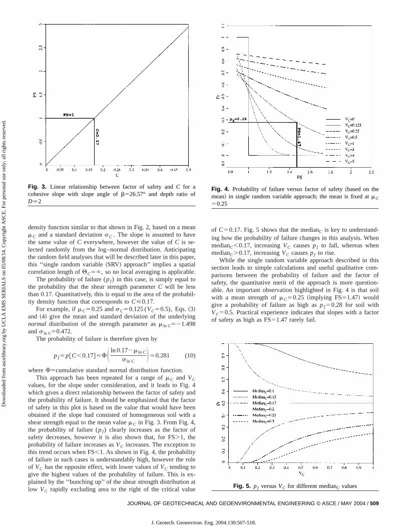
To put the probabilistic analyses into context, an initial deteristic study has been performed assuming a homogeneous sothe simple slope shown in Fig. 1, the factor of safety can rebe obtained from Taylor’s~1937! charts or simple limit equilibrium methods to give the data in Table 1.

These results, plotted in Fig. 3, indicate the linear relationbetweenC and FS. Fig. 3 also shows that the test slope becunstable when the shear strength parameter falls beloC50.17.

Single Random Variable Approach

The first probabilistic analysis presented here investigates th

Table 1. Factors of Safety Assuming Homogeneous Soil

C Factor of safety

0.15 0.880.17 1.000.20 1.180.25 1.470.30 1.77

fluence of giving the shear strengthC a log–normal probability

ERING © ASCE / MAY 2004

. 2004.130:507-518.

eanve

ingaper,alle.to

abil-

ying

ig. 4andctorbeenith a,of

toty

role

ex-n at

-henn

thiscom-r oftion-soil

actor

fet

Dow

nloa

ded

from

asc

elib

rary

.org

by

UC

LA

EM

S SE

RIA

LS

on 0

5/08

/14.

Cop

yrig

ht A

SCE

. For

per

sona

l use

onl

y; a

ll ri

ghts

res

erve

d.

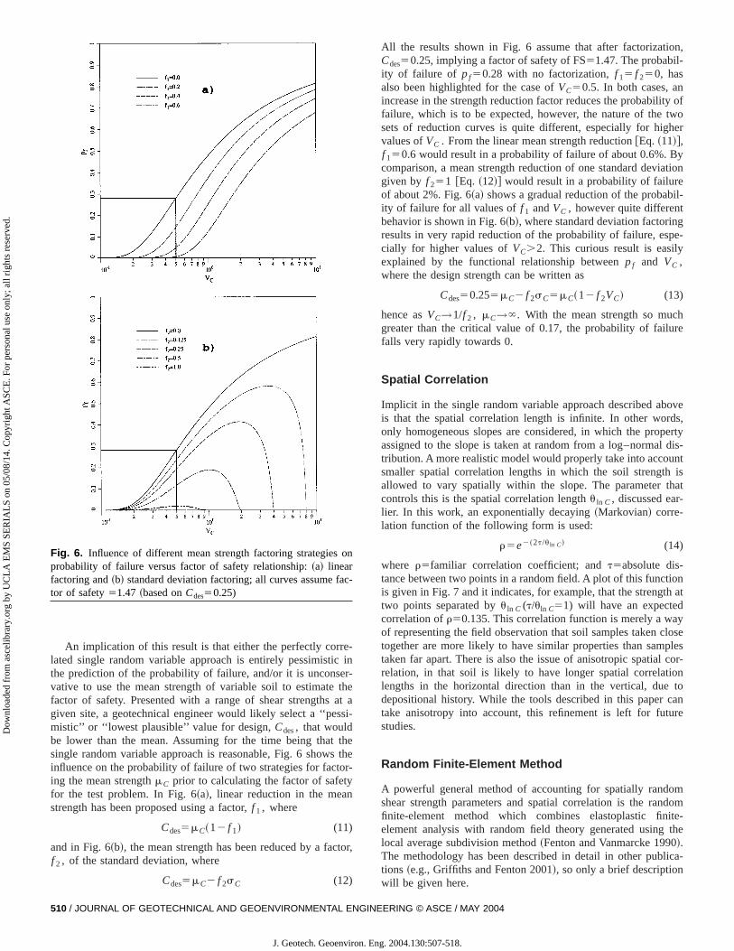
density function similar to that shown in Fig. 2, based on a mmC and a standard deviationsC . The slope is assumed to hathe same value ofC everywhere, however the value ofC is se-lected randomly from the log–normal distribution. Anticipatthe random field analyses that will be described later in this pthis ‘‘single random variable~SRV! approach’’ implies a spaticorrelation length ofQC5`, so no local averaging is applicab

The probability of failure (pf) in this case, is simply equalthe probability that the shear strength parameterC will be lessthan 0.17. Quantitatively, this is equal to the area of the probity density function that corresponds toC<0.17.

For example, ifmC50.25 andsC50.125 (VC50.5), Eqs.~3!and ~4! give the mean and standard deviation of the underlnormal distribution of the strength parameter asm ln C521.498ands ln C50.472.

The probability of failure is therefore given by

pf5p@C,0.17#5FS ln 0.172m ln C

s ln CD50.281 (10)

whereF5cumulative standard normal distribution function.This approach has been repeated for a range ofmC and VC

values, for the slope under consideration, and it leads to Fwhich gives a direct relationship between the factor of safetythe probability of failure. It should be emphasized that the faof safety in this plot is based on the value that would haveobtained if the slope had consisted of homogeneous soil wshear strength equal to the mean valuemC in Fig. 3. From Fig. 4the probability of failure (pf) clearly increases as the factorsafety decreases, however it is also shown that, for FS.1, theprobability of failure increases asVC increases. The exceptionthis trend occurs when FS,1. As shown in Fig. 4, the probabiliof failure in such cases is understandably high, however theof VC has the opposite effect, with lower values ofVC tending togive the highest values of the probability of failure. This isplained by the ‘‘bunching up’’ of the shear strength distributio

Fig. 3. Linear relationship between factor of safety andC for acohesive slope with slope angle ofb526.57° and depth ratio oD52

low VC rapidly excluding area to the right of the critical value



of C50.17. Fig. 5 shows that the medianC is key to understanding how the probability of failure changes in this analysis. WmedianC,0.17, increasingVC causespf to fall, whereas whemedianC.0.17, increasingVC causespf to rise.

While the single random variable approach described insection leads to simple calculations and useful qualitativeparisons between the probability of failure and the factosafety, the quantitative merit of the approach is more quesable. An important observation highlighted in Fig. 4 is thatwith a mean strength ofmC50.25 ~implying FS51.47! wouldgive a probability of failure as high aspf50.28 for soil withVC50.5. Practical experience indicates that slopes with a fof safety as high as FS51.47 rarely fail.

Fig. 4. Probability of failure versus factor of safety~based on thmean! in single random variable approach; the mean is fixed amC

50.25

Fig. 5. pf versusVC for different medianC values


. 2004.130:507-518.

re-tic iner-

e theat a

ssi-

t thes the

tor-tyn

ctor,

tion,l-

nlity oftwo

gher

Byiationebil-tngpe-

ily

chlure

boverds,pertyl dis-unt

th isthatr-

-tionth atdaycloseples

l cor-tion

tocan

ture

omndom

nite-the

0lica-n

s on

fac-

Dow

nloa

ded

from

asc

elib

rary

.org

by

UC

LA

EM

S SE

RIA

LS

on 0

5/08

/14.

Cop

yrig

ht A

SCE

. For

per

sona

l use

onl

y; a

ll ri

ghts

res

erve

d.

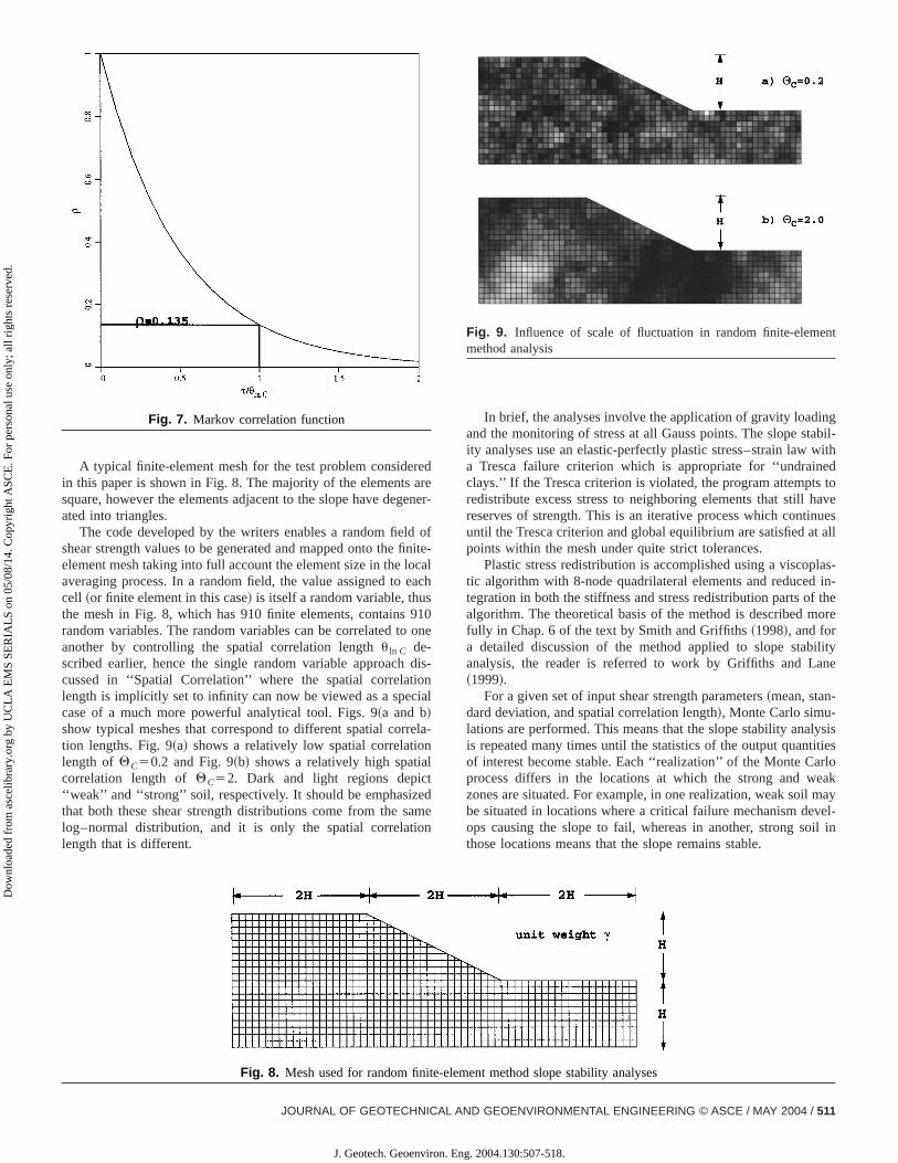
An implication of this result is that either the perfectly corlated single random variable approach is entirely pessimisthe prediction of the probability of failure, and/or it is unconsvative to use the mean strength of variable soil to estimatfactor of safety. Presented with a range of shear strengthsgiven site, a geotechnical engineer would likely select a ‘‘pemistic’’ or ‘‘lowest plausible’’ value for design,Cdes, that wouldbe lower than the mean. Assuming for the time being thasingle random variable approach is reasonable, Fig. 6 showinfluence on the probability of failure of two strategies for facing the mean strengthmC prior to calculating the factor of safefor the test problem. In Fig. 6~a!, linear reduction in the meastrength has been proposed using a factor,f 1 , where

Cdes5mC~12 f 1! (11)

and in Fig. 6~b!, the mean strength has been reduced by a faf 2 , of the standard deviation, where

C 5m 2 f s (12)

Fig. 6. Influence of different mean strength factoring strategieprobability of failure versus factor of safety relationship:~a! linearfactoring and~b! standard deviation factoring; all curves assumetor of safety51.47 ~based onCdes50.25)

des C 2 C



All the results shown in Fig. 6 assume that after factorizaCdes50.25, implying a factor of safety of FS51.47. The probabiity of failure of pf50.28 with no factorization,f 15 f 250, hasalso been highlighted for the case ofVC50.5. In both cases, aincrease in the strength reduction factor reduces the probabifailure, which is to be expected, however, the nature of thesets of reduction curves is quite different, especially for hivalues ofVC . From the linear mean strength reduction@Eq. ~11!#,f 150.6 would result in a probability of failure of about 0.6%.comparison, a mean strength reduction of one standard devgiven by f 251 @Eq. ~12!# would result in a probability of failurof about 2%. Fig. 6~a! shows a gradual reduction of the probaity of failure for all values off 1 andVC , however quite differenbehavior is shown in Fig. 6~b!, where standard deviation factoriresults in very rapid reduction of the probability of failure, escially for higher values ofVC.2. This curious result is easexplained by the functional relationship betweenpf and VC ,where the design strength can be written as

Cdes50.255mC2 f 2sC5mC~12 f 2VC! (13)

hence asVC→1/f 2 , mC→`. With the mean strength so mugreater than the critical value of 0.17, the probability of faifalls very rapidly towards 0.

Spatial Correlation

Implicit in the single random variable approach described ais that the spatial correlation length is infinite. In other woonly homogeneous slopes are considered, in which the proassigned to the slope is taken at random from a log–normatribution. A more realistic model would properly take into accosmaller spatial correlation lengths in which the soil strengallowed to vary spatially within the slope. The parametercontrols this is the spatial correlation lengthu ln C , discussed ealier. In this work, an exponentially decaying~Markovian! corre-lation function of the following form is used:

r5e2~2t/u ln C! (14)

where r5familiar correlation coefficient; andt5absolute distance between two points in a random field. A plot of this funcis given in Fig. 7 and it indicates, for example, that the strengtwo points separated byu ln C (t/uln C51) will have an expectecorrelation ofr50.135. This correlation function is merely a wof representing the field observation that soil samples takentogether are more likely to have similar properties than samtaken far apart. There is also the issue of anisotropic spatiarelation, in that soil is likely to have longer spatial correlalengths in the horizontal direction than in the vertical, duedepositional history. While the tools described in this papertake anisotropy into account, this refinement is left for fustudies.

Random Finite-Element Method

A powerful general method of accounting for spatially randshear strength parameters and spatial correlation is the rafinite-element method which combines elastoplastic fielement analysis with random field theory generated usinglocal average subdivision method~Fenton and Vanmarcke 199!.The methodology has been described in detail in other pubtions ~e.g., Griffiths and Fenton 2001!, so only a brief descriptio
will be given here.

. 2004.130:507-518.

eredare

gene

ld offinite

localeachs910

o one

dis-tioncial

rrela-onalctedsameion

ingtabil-with

nedts tohave

inuest all

plas-d in-f the

more

bilityane

--alysistitiesarloeak

l mayevel-oil in

ent

Dow

nloa

ded

from

asc

elib

rary

.org

by

UC

LA

EM

S SE

RIA

LS

on 0

5/08

/14.

Cop

yrig

ht A

SCE

. For

per

sona

l use

onl

y; a

ll ri

ghts

res

erve

d.

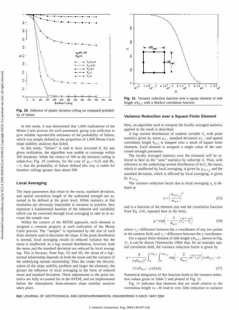
A typical finite-element mesh for the test problem considin this paper is shown in Fig. 8. The majority of the elementssquare, however the elements adjacent to the slope have deated into triangles.

The code developed by the writers enables a random fieshear strength values to be generated and mapped onto theelement mesh taking into full account the element size in theaveraging process. In a random field, the value assigned tocell ~or finite element in this case! is itself a random variable, thuthe mesh in Fig. 8, which has 910 finite elements, containsrandom variables. The random variables can be correlated tanother by controlling the spatial correlation lengthu ln C de-scribed earlier, hence the single random variable approachcussed in ‘‘Spatial Correlation’’ where the spatial correlalength is implicitly set to infinity can now be viewed as a specase of a much more powerful analytical tool. Figs. 9~a and b!show typical meshes that correspond to different spatial cotion lengths. Fig. 9~a! shows a relatively low spatial correlatilength of QC50.2 and Fig. 9~b! shows a relatively high spaticorrelation length ofQC52. Dark and light regions depi‘‘weak’’ and ‘‘strong’’ soil, respectively. It should be emphasizthat both these shear strength distributions come from thelog–normal distribution, and it is only the spatial correlatlength that is different.

Fig. 7. Markov correlation function

Fig. 8. Mesh used for random fin



r-

-

In brief, the analyses involve the application of gravity loadand the monitoring of stress at all Gauss points. The slope sity analyses use an elastic-perfectly plastic stress–strain lawa Tresca failure criterion which is appropriate for ‘‘undraiclays.’’ If the Tresca criterion is violated, the program attempredistribute excess stress to neighboring elements that stillreserves of strength. This is an iterative process which contuntil the Tresca criterion and global equilibrium are satisfied apoints within the mesh under quite strict tolerances.

Plastic stress redistribution is accomplished using a viscotic algorithm with 8-node quadrilateral elements and reducetegration in both the stiffness and stress redistribution parts oalgorithm. The theoretical basis of the method is describedfully in Chap. 6 of the text by Smith and Griffiths~1998!, and fora detailed discussion of the method applied to slope staanalysis, the reader is referred to work by Griffiths and L~1999!.

For a given set of input shear strength parameters~mean, standard deviation, and spatial correlation length!, Monte Carlo simulations are performed. This means that the slope stability anis repeated many times until the statistics of the output quanof interest become stable. Each ‘‘realization’’ of the Monte Cprocess differs in the locations at which the strong and wzones are situated. For example, in one realization, weak soibe situated in locations where a critical failure mechanism dops causing the slope to fail, whereas in another, strong sthose locations means that the slope remains stable.

ement method slope stability analyses

Fig. 9. Influence of scale of fluctuation in random finite-elemmethod analysis

ite-el


. 2004.130:507-518.

thent toure,arlo

nyithing is

for

iatione as-thistheybility

ac-

t isonte

eachtion

t thebothverag–ce ofreti-, theced

nt stantedlysis

tistics

lnite

und-

re-

,

iven

ction

ts..-

duc-

the

bil-

side

Dow

nloa

ded

from

asc

elib

rary

.org

by

UC

LA

EM

S SE

RIA

LS

on 0

5/08

/14.

Cop

yrig

ht A

SCE

. For

per

sona

l use

onl

y; a

ll ri

ghts

res

erve

d.

In this study, it was determined that 1,000 realizations ofMonte Carlo process for each parametric group was sufficiegive reliable reproducible estimates of the probability of failwhich was simply defined as the proportion of 1,000 Monte Cslope stability analyses that failed.

In this study, ‘‘failure’’ is said to have occurred if, for agiven realization, the algorithm was unable to converge w500 iterations. While the choice of 500 as the iteration ceilinsubjective, Fig. 10 confirms, for the case ofmC50.25 andQC

51, that the probability of failure defined this way is stableiteration ceilings greater than about 200.

Local Averaging

The input parameters that relate to the mean, standard devand spatial correlation length of the undrained strength arsumed to be defined at the point level. While statistics atresolution are obviously impossible to measure in practice,represent a fundamental baseline of the inherent soil variawhich can be corrected through local averaging to take in tocount the sample size.

Within the context of the RFEM approach, each elemenassigned a constant property at each realization of the MCarlo process. The ‘‘sample’’ is represented by the size offinite element used to discretize the slope. If the point distribuis normal, local averaging results in reduced variance bumean is unaffected. In a log–normal distribution, however,the mean and the standard deviation are reduced by local aing. This is because, from Eqs.~5! and ~6!, the mean of a lognormal relationship depends on both the mean and the varianthe underlying normal relationship. Thus the cruder the disczation of the slope stability problem and larger the elementsgreater the influence of local averaging in the form of redumean and standard deviation. These adjustments to the poitistics are fully accounted for in the RFEM, and are implemebefore the elastoplastic finite-element slope stability ana

Fig. 10. Influence of plastic iteration ceiling on computed probaity of failure

takes place.



,

-

-

Variance Reduction over a Square Finite Element

Here, an algorithm used to compute the locally averaged staapplied to the mesh is described.

A log–normal distribution of random variableC, with pointstatistics given by meanmC , standard deviationsC , and spatiacorrelation lengthu ln C is mapped onto a mesh of square fielements. Each element is assigned a single value of therained strength parameter.

The locally averaged statistics over the elements will beferred to here as the ‘‘area’’ statistics by subscriptA. Thus, withreference to the underlying normal distribution of lnC, the meanwhich is unaffected by local averaging, is given bym ln CA

, and thestandard deviation, which is affected by local averaging, is gby s ln CA

.The variance reduction factor due to local averagingg, is de-

fined as

g5S s ln CA

s ln CD 2

(15)

and is a function of the element size and the correlation funfrom Eq. ~14!, repeated here in the form,

r5expS 22

u ln CAtx

21ty2D (16)

wheretx5difference between thex coordinates of any two poinin the random field; andty5difference between they coordinates

For a square finite element of side lengthau ln C , shown in Fig11, it can be shown~Vanmarcke 1984! that, for an isotropic spatial correlation field, the variance reduction factor is given by

g54

~au ln C!4 E0

au ln CE0

au ln C

expS 22

u ln CAx21y2D ~au ln C2x!

3~au ln C2y!dxdy (17)

Numerical integration of this function leads to the variance retion values given in Table 2 and plotted in Fig. 11.

Fig. 11 indicates that elements that are small relative to

Fig. 11. Variance reduction function over a square element oflengthau ln C with a Markov correlation function

correlation length~a→0! lead to very little reduction in variance


. 2004.130:507-518.

ation

er-

ld,ite-

tics,ation

Ran-

thes of

hfor

ngthle toativet, andlly

ined

ll

e of a

ribu-

nds

omging

allyref-ave ail-t

cally

ethe

theer

size

Dow

nloa

ded

from

asc

elib

rary

.org

by

UC

LA

EM

S SE

RIA

LS

on 0

5/08

/14.

Cop

yrig

ht A

SCE

. For

per

sona

l use

onl

y; a

ll ri

ghts

res

erve

d.

~g→1!, whereas elements that are large relative to the correllength can lead to very significant variance reduction~g→0!.

The statistics of the underlying log field, including local avaging, are therefore given by

s ln CA5s ln CAg (18)

and

m ln CA5m ln C (19)

which leads to the following statistics of the log–normal fieincluding local averaging, that is actually mapped on the finelement mesh from Eqs.~5! and ~6!, thus

mCA5exp~m ln CA

1 12s ln CA

2 ! (20)

sCA5mCA

Aexp~s ln CA

2 !21 (21)

It is instructive to consider the range of locally averaged statissince this helps to explain the influence of the spatial correllength QC(5u ln C /H) on the probability of failure in the RFEMslope analyses that is described in ‘‘Locally Averaged Singledom Variable Approach.’’

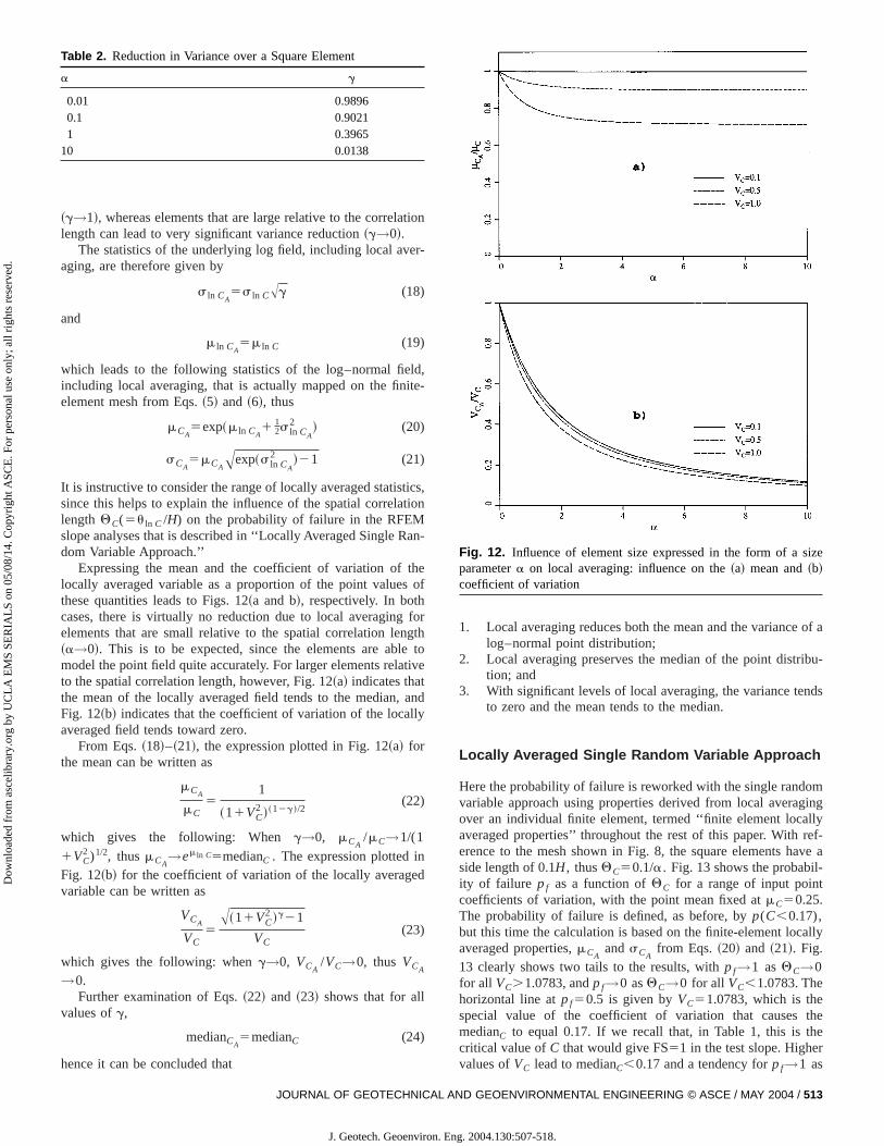
Expressing the mean and the coefficient of variation oflocally averaged variable as a proportion of the point valuethese quantities leads to Figs. 12~a and b!, respectively. In botcases, there is virtually no reduction due to local averagingelements that are small relative to the spatial correlation le~a→0!. This is to be expected, since the elements are abmodel the point field quite accurately. For larger elements relto the spatial correlation length, however, Fig. 12~a! indicates thathe mean of the locally averaged field tends to the medianFig. 12~b! indicates that the coefficient of variation of the locaaveraged field tends toward zero.

From Eqs.~18!–~21!, the expression plotted in Fig. 12~a! forthe mean can be written as

mCA

mC5

1

~11VC2 !~12g!/2

(22)

which gives the following: When g→0, mCA/mC→1/(1

1VC2 )1/2, thusmCA

→em ln C5medianC . The expression plottedFig. 12~b! for the coefficient of variation of the locally averagvariable can be written as

VCA

VC5

A~11VC2 !g21

VC(23)

which gives the following: wheng→0, VCA/VC→0, thus VCA

→0.Further examination of Eqs.~22! and ~23! shows that for a

values ofg,

medianCA5medianC (24)

Table 2. Reduction in Variance over a Square Element

a g

0.01 0.98960.1 0.90211 0.3965

10 0.0138

hence it can be concluded that



1. Local averaging reduces both the mean and the varianclog–normal point distribution;

2. Local averaging preserves the median of the point disttion; and

3. With significant levels of local averaging, the variance teto zero and the mean tends to the median.

Locally Averaged Single Random Variable Approach

Here the probability of failure is reworked with the single randvariable approach using properties derived from local averaover an individual finite element, termed ‘‘finite element locaveraged properties’’ throughout the rest of this paper. Witherence to the mesh shown in Fig. 8, the square elements hside length of 0.1H, thusQC50.1/a. Fig. 13 shows the probabity of failure pf as a function ofQC for a range of input poincoefficients of variation, with the point mean fixed atmC50.25.The probability of failure is defined, as before, byp(C,0.17),but this time the calculation is based on the finite-element loaveraged properties,mCA

andsCAfrom Eqs.~20! and ~21!. Fig.

13 clearly shows two tails to the results, withpf→1 asQC→0for all VC.1.0783, andpf→0 asQC→0 for all VC,1.0783. Thehorizontal line atpf50.5 is given byVC51.0783, which is thspecial value of the coefficient of variation that causesmedianC to equal 0.17. If we recall that, in Table 1, this iscritical value ofC that would give FS51 in the test slope. High

Fig. 12. Influence of element size expressed in the form of aparametera on local averaging: influence on the~a! mean and~b!coefficient of variation

values ofVC lead to medianC,0.17 and a tendency forpf→1 as


. 2004.130:507-518.

therlyf 0

orre-ty.

sec-aseds de-n in

ntemetric

m is15

iated-

aly-onesned

ation,urallyveryp-radi-

beicularing

7fig.lure

ob-wasite-e re-effi-

the

ging

atefgle

sedd at

sedd at

h at

Dow

nloa

ded

from

asc

elib

rary

.org

by

UC

LA

EM

S SE

RIA

LS

on 0

5/08

/14.

Cop

yrig

ht A

SCE

. For

per

sona

l use

onl

y; a

ll ri

ghts

res

erve

d.

QC→0. Conversely, lower values ofVC lead to medianC.0.17and a tendency forpf→0. Fig. 14 shows the same data plottedother way round withVC along the abscissa. Fig. 14 cleashows the full influence of spatial correlation in the range o<QC,`. All the curves cross over at the critical value ofVC

51.0783, and it is of interest to note the step function that csponds toQC50 whenpf changes suddenly from zero to uni

It should be emphasized that the results presented in thistion involved no actual finite-element analysis, and were bsolely on a SRV approach using locally averaged propertierived from a typical finite element in a mesh such as that showFig. 8.

Fig. 13. Probability of failure versus spatial correlation length baon finite-element locally averaged properties; the mean is fixemC50.25

Fig. 14. Probability of failure versus coefficient of variation baon finite-element locally averaged properties; the mean is fixemC50.25



Results of Random Finite-Element Method Analyses

Now, the results of full nonlinear RFEM analyses with MoCarlo simulations are described based on a range of paravariations ofmC , VC , andQC .

In the elastoplastic RFEM approach, the failure mechanisfree to ‘‘seek out’’ the weakest path through the soil. Fig.shows two typical random field realizations and the assocfailure mechanisms for slopes withQC50.5 and 2. The convoluted nature of the failure mechanisms, especially whenQC

50.5, would defy analysis by conventional slope stability ansis tools. While the mechanism is attracted to the weaker zwithin the slope, it will inevitably pass through elements assigmany different strength values. This weakest path determinand the strength averaging that goes with it, occurs quite natin the finite-element slope stability method, and represents asignificant improvement over traditional limit equilibrium aproaches to probabilistic slope stability analysis. In these ttional methods, if local averaging is included at all, it has tocomputed over a failure mechanism that is preset by the partanalysis method~e.g., a circular failure mechanism when usBishop’s method!.

In fixing the point mean strength atmC50.25, Figs. 16 and 1show the effect of spatial correlation lengthQC and coefficient ovariationVC on the probability of failure for the test problem. F16 clearly indicates two branches, with the probability of faitending toward unity or zero for higher and lower values ofVC ,respectively. This behavior is qualitatively similar to thatserved in Fig. 13, in which a single random variable approachused to predict the probability of failure based solely on finelement locally averaged properties. Fig. 17 shows the samsults as Fig. 16, but plotted the other way round with the cocient of variation along the abscissa. Fig. 17 also showstheoretically obtained result corresponding toQC5`, indicatingthat a single random variable approach with no local averawill overestimate the probability of failure~conservative! whenthe coefficient of variation is relatively small and underestimthe probability of failure~unconservative! when the coefficient ovariation is relatively high. Fig. 17 also confirms that the sin

Fig. 15. Typical random field realizations and deformed messlope failure for two different spatial correlation lengths

random variable approach described earlier in the paper, which


. 2004.130:507-518.

howthis

ghtsility,allyak-s re-

ver

ate-

-omese

16: it

entnts in

theh the

tore-

of thewith

nd a

er-lution

he

domtest

-

5.n. 20

ows

om

m

an-gingent

Dow

nloa

ded

from

asc

elib

rary

.org

by

UC

LA

EM

S SE

RIA

LS

on 0

5/08

/14.

Cop

yrig

ht A

SCE

. For

per

sona

l use

onl

y; a

ll ri

ghts

res

erve

d.

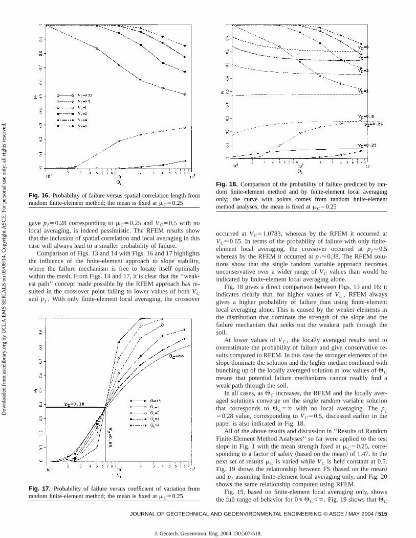
gavepf50.28 corresponding tomC50.25 andVC50.5 with nolocal averaging, is indeed pessimistic. The RFEM results sthat the inclusion of spatial correlation and local averaging incase will always lead to a smaller probability of failure.

Comparison of Figs. 13 and 14 with Figs. 16 and 17 highlithe influence of the finite-element approach to slope stabwhere the failure mechanism is free to locate itself optimwithin the mesh. From Figs. 14 and 17, it is clear that the ‘‘weest path’’ concept made possible by the RFEM approach hasulted in the crossover point falling to lower values of bothVC

and pf . With only finite-element local averaging, the crosso

Fig. 16. Probability of failure versus spatial correlation length frrandom finite-element method; the mean is fixed atmC50.25

Fig. 17. Probability of failure versus coefficient of variation frorandom finite-element method; the mean is fixed atmC50.25



occurred atVC51.0783, whereas by the RFEM it occurredVC'0.65. In terms of the probability of failure with only finitelement local averaging, the crossover occurred atpf50.5whereas by the RFEM it occurred atpf'0.38. The RFEM solutions show that the single random variable approach becunconservative over a wider range ofVC values than would bindicated by finite-element local averaging alone.

Fig. 18 gives a direct comparison between Figs. 13 andindicates clearly that, for higher values ofVC , RFEM alwaysgives a higher probability of failure than using finite-elemlocal averaging alone. This is caused by the weaker elemethe distribution that dominate the strength of the slope andfailure mechanism that seeks out the weakest path througsoil.

At lower values ofVC , the locally averaged results tendoverestimate the probability of failure and give conservativesults compared to RFEM. In this case the stronger elementsslope dominate the solution and the higher median combinedbunching up of the locally averaged solution at low values ofQC

means that potential failure mechanisms cannot readily fiweak path through the soil.

In all cases, asQC increases, the RFEM and the locally avaged solutions converge on the single random variable sothat corresponds toQC5` with no local averaging. Thepf

50.28 value, corresponding toVC50.5, discussed earlier in tpaper is also indicated in Fig. 18.

All of the above results and discussion in ‘‘Results of RanFinite-Element Method Analyses’’ so far were applied to theslope in Fig. 1 with the mean strength fixed atmC50.25, corresponding to a factor of safety~based on the mean! of 1.47. In thenext set of resultsmC is varied whileVC is held constant at 0.Fig. 19 shows the relationship between FS~based on the mea!andpf assuming finite-element local averaging only, and Figshows the same relationship computed using RFEM.

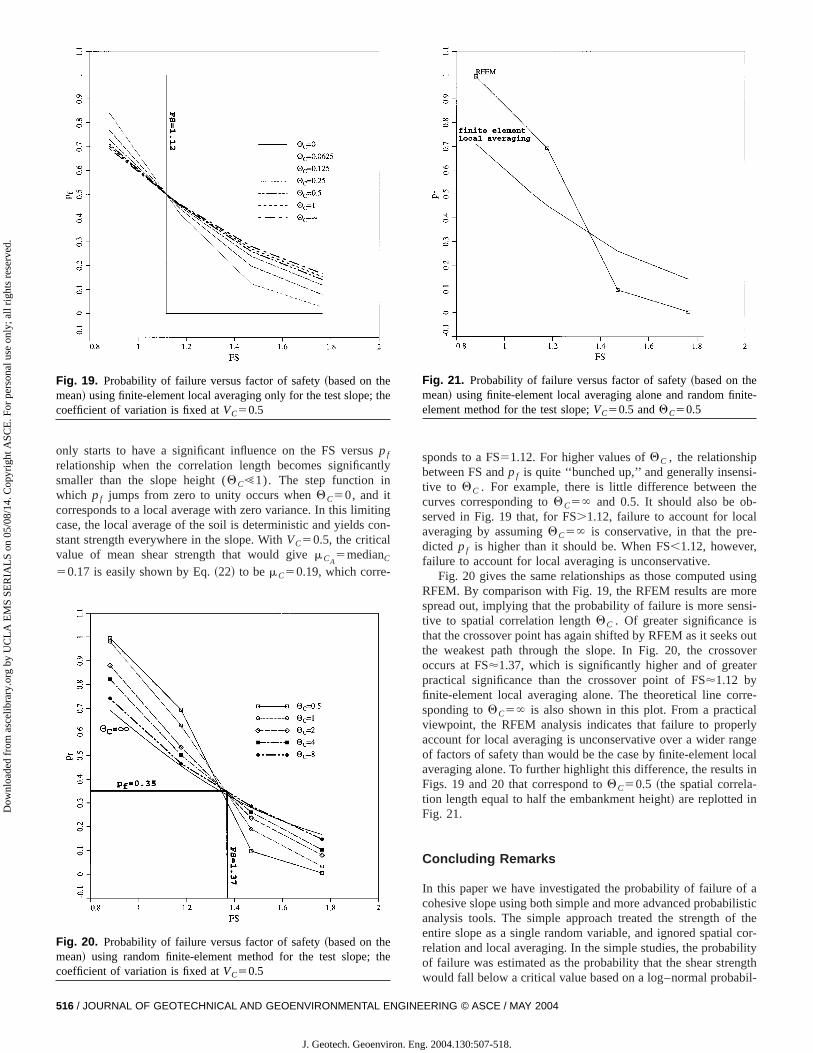
Fig. 19, based on finite-element local averaging only, sh

Fig. 18. Comparison of the probability of failure predicted by rdom finite-element method and by finite-element local averaonly; the curve with points comes from random finite-elemmethod analyses; the mean is fixed atmC50.25

the full range of behavior for 0<QC,`. Fig. 19 shows thatQC


. 2004.130:507-518.

sntly

n

itingcon-

l

-

psi-theb-ale-r,

usingorensi-iss out

soverter

orre-calerlyangelocallts in-

of ailisticf thel cor-bilityength

e; the

ethe

enite-

Dow

nloa

ded

from

asc

elib

rary

.org

by

UC

LA

EM

S SE

RIA

LS

on 0

5/08

/14.

Cop

yrig

ht A

SCE

. For

per

sona

l use

onl

y; a

ll ri

ghts

res

erve

d.

only starts to have a significant influence on the FS versupf

relationship when the correlation length becomes significasmaller than the slope height (QC!1). The step function iwhich pf jumps from zero to unity occurs whenQC50, and itcorresponds to a local average with zero variance. In this limcase, the local average of the soil is deterministic and yieldsstant strength everywhere in the slope. WithVC50.5, the criticavalue of mean shear strength that would givemCA

5medianC50.17 is easily shown by Eq.~22! to bemC50.19, which corre

Fig. 19. Probability of failure versus factor of safety~based on thmean! using finite-element local averaging only for the test slopecoefficient of variation is fixed atVC50.5

Fig. 20. Probability of failure versus factor of safety~based on thmean! using random finite-element method for the test slope;coefficient of variation is fixed atVC50.5



sponds to a FS51.12. For higher values ofQC , the relationshibetween FS andpf is quite ‘‘bunched up,’’ and generally insentive to QC . For example, there is little difference betweencurves corresponding toQC5` and 0.5. It should also be oserved in Fig. 19 that, for FS.1.12, failure to account for locaveraging by assumingQC5` is conservative, in that the prdicted pf is higher than it should be. When FS,1.12, howevefailure to account for local averaging is unconservative.

Fig. 20 gives the same relationships as those computedRFEM. By comparison with Fig. 19, the RFEM results are mspread out, implying that the probability of failure is more setive to spatial correlation lengthQC . Of greater significancethat the crossover point has again shifted by RFEM as it seekthe weakest path through the slope. In Fig. 20, the crosoccurs at FS'1.37, which is significantly higher and of greapractical significance than the crossover point of FS'1.12 byfinite-element local averaging alone. The theoretical line csponding toQC5` is also shown in this plot. From a practiviewpoint, the RFEM analysis indicates that failure to propaccount for local averaging is unconservative over a wider rof factors of safety than would be the case by finite-elementaveraging alone. To further highlight this difference, the resuFigs. 19 and 20 that correspond toQC50.5 ~the spatial correlation length equal to half the embankment height! are replotted inFig. 21.

Concluding Remarks

In this paper we have investigated the probability of failurecohesive slope using both simple and more advanced probabanalysis tools. The simple approach treated the strength oentire slope as a single random variable, and ignored spatiarelation and local averaging. In the simple studies, the probaof failure was estimated as the probability that the shear str

Fig. 21. Probability of failure versus factor of safety~based on thmean! using finite-element local averaging alone and random fielement method for the test slope;VC50.5 andQC50.5

would fall below a critical value based on a log–normal probabil-


. 2004.130:507-518.

ap-eter-thatof

finitelasto-takeob-

etricthod

of theant

ysisuree soiligher

ging

tiald to

ffect

ely

studys in

the

to

sis

snd

gto

d

-g.,

al

a

hnite,

y-

e

,.,

h

iler-

75.r-

gn

Dow

nloa

ded

from

asc

elib

rary

.org

by

UC

LA

EM

S SE

RIA

LS

on 0

5/08

/14.

Cop

yrig

ht A

SCE

. For

per

sona

l use

onl

y; a

ll ri

ghts

res

erve

d.

ity density function. These results led to a discussion on thepropriate choice of design shear strength value suitable for dministic analysis. Two factorization methods were proposedwere able to bring the probability of failure and the factorsafety more into line with practical experience.

The second half of the paper implemented the randomelement method on the same test problem. The nonlinear eplastic analyses with Monte Carlo simulation were able tointo full account spatial correlation and local averaging, andserve their impact on the probability of failure using a paramapproach. The elastoplastic finite-element slope stability memakes no a priori assumptions about the shape or locationcritical failure mechanism, and therefore offers very significbenefits over traditional limit equilibrium methods in the analof highly variable soils. In the elastoplastic RFEM, the failmechanism is free to seek out the weakest path through thand it has been shown that this phenomenon can lead to hprobabilities of failure than could be explained by local averaalone.

In summary, simplified probabilistic analysis, in which spavariability is ignored by assuming perfect correlation, can leaunconservative estimates of the probability of failure. This eis most pronounced at relatively low factors of safety~Fig. 20! orwhen the coefficient of variation of the soil strength is relativhigh ~Fig. 18!.

Acknowledgment

The results shown in this paper are part of a much broaderinto the influence of soil heterogeneity on stability problemgeotechnical engineering. The writers wish to acknowledgesupport of NSF Grant No. CMS-9877189.

Notation

The following symbols were used in this paper:C 5 dimensionless shear strength;

Cdes 5 design value ofC;cu 5 undrained shear strength;D 5 foundation depth ratio;f 1 5 linear strength reduction factor;f 2 5 strength reduction factor based on standard

deviation;H 5 height of slope;pf 5 probability of failure;

VC 5 coefficient of variation ofC;x 5 Cartesianx coordinate;y 5 Cartesiany coordinate;a 5 dimensionless element size parameter;b 5 slope angle;g 5 variance reduction factor;

gsat 5 saturated unit weight;QC 5 dimensionless spatial correlation length of lnC;uC 5 spatial correlation length ofC;

u ln C 5 spatial correlation length of lnC;mC 5 mean ofC;

mCA 5 locally averaged mean ofC over a square finiteelement;

m ln C 5 mean of lnC;m ln CA5 locally averaged mean of lnC over a square finite

element;
r 5 correlation coefficient;


sC 5 standard deviation ofC;sCA 5 locally averaged standard deviation ofC over a

square finite element;s ln C 5 standard deviation of lnCs ln CA 5 locally averaged standard deviation of lnC over a

square finite element;t 5 absolute distance between two points;

tx 5 x-component of distance between two points;ty 5 y-component of distance between two points; andfu 5 undrained friction angle.

References

Alonso, E. E. ~1976!. ‘‘Risk analysis of slopes and its applicationslopes in Canadian sensitive clays.’’Geotechnique,26, 453–472.

Bishop, A. W.~1955!. ‘‘The use of the slip circle in the stability analyof slopes.’’Geotechnique,5~1!, 7–17.

Chowdhury, R. N., and Tang, W. H.~1987!. ‘‘Comparison of risk modelfor slopes.’’ Proc., 5th Int. Conf. on Applications of Statistics aProbability in Soil and Structural Engineering, 2, 863–869.

Christian, J. T.~1996!. ‘‘Reliability methods for stability of existinslopes.’’ Uncertainty in the geologic environment: From theorypractice, Geotechnical Special Publication No. 58, C. D. Shackelforet al., eds., ASCE, New York, 409–418.

Christian, J. T., Ladd, C. C., and Baecher, G. B.~1994!. ‘‘Reliabilityapplied to slope stability analysis.’’J. Geotech. Eng.,120~12!, 2180–2207.

D’Andrea, R. A., and Sangrey, D. A.~1982!. ‘‘Safety factors for probabilistic slope design.’’J. Geotech. Eng. Div., Am. Soc. Civ. En108~9!, 1108–1118.

Duncan, J. M.~2000!. ‘‘Factors of safety and reliability in geotechnicengineering.’’J. Geotech. Geoenviron. Eng.,126~4!, 307–316.

El-Ramly, H., Morgenstern, N. R., and Cruden, D. M.~2002!. ‘‘Probabi-listic slope stability analysis for practice.’’Can. Geotech. J.,39, 665–683.

Fenton, G. A., and Griffiths, D. V.~1993!. ‘‘Statistics of flow throughsimple bounded stochastic medium.’’Water Resour. Res.,29~6!,1825–1830.

Griffiths, D. V., and Fenton, G. A.~2000!. ‘‘Influence of soil strengtspatial variability on the stability of an undrained clay slope by fielements.’’Slope Stability 2000, Proc., GeoDenver 2000, 184–193ASCE, New York.

Griffiths, D. V., and Fenton, G. A.~2001!. ‘‘Bearing capacity of spatiallrandom soil: The undrained clay Prandtl problem revisited.’’Geotechnique,51~4!, 351–359.

Griffiths, D. V., and Lane, P. A.~1999!. ‘‘Slope stability analysis by finitelements.’’Geotechnique,49~3!, 387–403.

Fenton, G. A., and Vanmarcke, E. H.~1990!. ‘‘Simulation of randomfields via local average subdivision.’’J. Eng. Mech.,116~8!, 1733–1749.

Hassan, A. M., and Wolff, T. F.~2000!. ‘‘Effect of deterministic andprobabilistic models on slope reliability index.’’Slope Stability 2000Geotechnical Special Publication No. 101, D. V. Griffiths et al., edsASCE, New York, 194–208.

Kulhawy, F. H., Roth, M. J. S., and Grigoriu, M. D.~1991!. ‘‘Somestatistical evaluations of geotechnical properties.’’Proc., ICASP6, 6tInt. Conf. on Applied Statistics Probability in Civil Engineering.

Lacasse, S.~1994!. ‘‘Reliability and probabilistic methods.’’Proc., 13thInt. Conf. on Soil Mechanics Foundation Engineering, 225–227.

Lacasse, S., and Nadim, F.~1996!. ‘‘Uncertainties in characterising soproperties.’’Geotechnical Special Publication No. 58, Proc., Unctainity ’96, C. D. Shackelford et al., eds., ASCE, New York, 49–

Lee, I. K., White, W., and Ingles, O. G.~1983!. Geotechnical engineeing, Pitman, London.

Li, K. S., and Lumb, P.~1987!. ‘‘Probabilistic design of slopes.’’Can.Geotech. J.,24, 520–531.

Matsuo, M., and Kuroda, K.~1974!. ‘‘Probabilistic approach to the desi
of embankments.’’Soils Found.,14~1!, 1–17.

. 2004.130:507-518.

eEn-tter-

eon

hD

nt

v.

.

o-

.’’ice,l.,

Dow

nloa

ded

from

asc

elib

rary

.org

by

UC

LA

EM

S SE

RIA

LS

on 0

5/08

/14.

Cop

yrig

ht A

SCE

. For

per

sona

l use

onl

y; a

ll ri

ghts

res

erve

d.

Mostyn, G. R., and Li, K. S.~1993!. ‘‘Probabilistic slope stability—Statof play.’’ Proc., Conf. on Probabilistic Methods in Geotechnicalgineering, K. S. Li and S.-C. R. Lo, eds., 89–110, Balkema, Rodam, The Netherlands.

Mostyn, G. R., and Soo, S.~1992!. ‘‘The effect of autocorrelation on thprobability of failure of slopes.’’6th Australia, New Zealand Conf.Geomechanics: Geotechnical Risk, 542–546.

Paice, G. M.~1997!. ‘‘Finite element analysis of stochastic soils.’’ Pthesis, Univ. of Manchester, Manchester, U.K.

Smith, I. M., and Griffiths, D. V.~1998!. Programming the finite elememethod, 3rd Ed., Wiley, Chichester, U.K.

Tang, W. H., Yucemen, M. S., and Ang, A. H. S.~1976!. ‘‘Probability-
based short-term design of slopes.’’Can. Geotech. J.,13, 201–215.


Taylor, D. W. ~1937!. ‘‘Stability of earth slopes.’’J. Boston Soc. CiEng.,24, 197–246.

Vanmarcke, E. H.~1977!. ‘‘Reliability of earth slopes.’’J. Geotech. EngDiv., Am. Soc. Civ. Eng.,103~11!, 1247–1265.

Vanmarcke, E. H.~1984!. Random fields: Analysis and synthesis, MITPress, Cambridge, Mass.

Whitman, R. V.~2000!. ‘‘Organizing and evaluating uncertainty in getechnical engineering.’’J. Geotech. Geoenviron. Eng.,126~7!, 583–593.

Wolff, T. F. ~1996!. ‘‘Probabilistic slope stability in theory and practiceUncertainty in the geologic environment: From theory to practGeotechnical Special Publication No. 58, C. D. Shackelford et a
eds., ASCE, New York, 419–433.

. 2004.130:507-518.

Documents

Probabilistic Slope Stability Analysis by Finite Elements