Embed Size (px)
Citation preview
85
5.1 INTRODUCTION
Probabilistic reliability evaluation is the most important activity in probabilistic trans-mission planning. In reliability evaluation, the load models in Chapter 3 and the system analysis techniques in Chapter 4 are combined with probabilistic system state selection methods to create reliability indices that truly represent the system reliability level. Some indices can be converted into monetary values so that the reliability worth based on the indices and the economic assessment of investment and operation costs could be performed on a unifi ed valuation basis.
Reliability evaluation is divided into two areas of the system adequacy and system security: Adequacy relates to the existence of suffi cient facilities within the system to satisfy the load demand and system operational constraints, and is therefore associated with static conditions. Security relates to the ability of the system to respond to dynamic disturbances arising within the system and is therefore associated with the dynamic conditions that may cause transient or voltage instability.
Probabilistic reliability evaluation includes four aspects:
• Reliability data
• Reliability indices
5
PROBABILISTIC RELIABILITY EVALUATION
Probabilistic Transmission System Planning, by Wenyuan LiCopyright © 2011 Institute of Electrical and Electronics Engineers
c05.indd 85c05.indd 85 1/20/2011 10:25:45 AM1/20/2011 10:25:45 AM
86 PROBABILISTIC RELIABILITY EVALUATION
• Reliability worth assessment
• Reliability evaluation models and methods
Reliability data will be discussed with other data for transmission planning in Chapter 7 . The defi nitions of reliability indices are discussed in Section 5.2 and the basic con-cepts of reliability worth assessment, in Section 5.3 . Adequacy evaluation techniques for substation confi gurations and composite systems are described in Sections 5.4 and 5.5 , respectively. Security assessments, which are divided into probabilistic voltage stability and probabilistic transient stability, are presented in Sections 5.6 and 5.7 , respectively.
5.2 RELIABILITY INDICES
Reliability indices can be classifi ed into two categories:
1. Indices used to estimate the reliability level of a future system with various changes, including load growth, change in operation conditions, modifi cation or enhancement in network confi guration, and addition or retirement of facilities in the system.
2. Indices used to measure the historical performance of the existing system or equipment
The reliability indices discussed in this section pertain to category 1. Category 2 indices will be addressed in Chapter 7 as part of the data required in probabilistic transmission planning.
There are many possible indices that can be used to measure transmission system reliability. Most reliability indices are the expected values of random variables, although a probability distribution can be calculated in some cases. It is important to appreciate that an expected value is not a deterministic quantity. It is the long time average of the phenomenon under study. The expected indices provide the average outcomes due to various factors such as system component availability or failure probability, component capacities, load characteristics and uncertainty, system topological confi gurations, and operational conditions.
5.2.1 Adequacy Indices
The six adequacy indices are as follows:
1. Probability of Load Curtailments ( PLC ) . This is expressed as
PLC =∈∑ pi
i S
(5.1)
where p i is the probability of the system state i and S is the set of all system states associated with load curtailments.
c05.indd 86c05.indd 86 1/20/2011 10:25:45 AM1/20/2011 10:25:45 AM
5.2 RELIABILITY INDICES 87
2. Expected Frequency of Load Curtailments ( EFLC ) . This is expressed (in outages per year) as
EFLC = −∈∑ ( )F fi i
i S
(5.2)
where F i is the frequency of entering (or departing) the load curtailment state i and f i is the portion of F i that corresponds to not passing through the boundary wall between the load curtailment state set and non - load - curtailment state set. In other words, f i is the frequency of transition from other load curtailment states to the load curtailment state i . In using a state enumeration or state sampling (nonsequential Monte Carlo simulation) technique, it is diffi cult or extremely time - consuming to identify all transitions between load curtailment states. The ENLC (expected number of load curtailments) index is often used to approxi-mate the EFLC:
ENLC =∈∑Fi
i S
(5.3)
It can be seen that f i is ignored in calculating the ENLC and therefore the ENLC is an upper - bound estimate of the EFLC. This approximation is generally acceptable in transmission reliability evaluation because the probability of tran-sitions from one load curtailment state to another is small. In most cases, the system transits from a load curtailment state to the normal operation (non - load - curtailment) state by a repairing or recovering process. The system state fre-quency F i can be calculated by
F pi i k
k Ni
=∈∑λ (5.4)
where λ k is the k th departure rate of components in system state i and N i is the set of all possible departure rates in the system state i . For example, if a com-ponent in system state i is in the normal state, the departure rate is its outage rate, whereas if it is in an outage state, the departure rate is its repair or recovery rate. A component may be represented by a multistate model such as the one including not only up and down states but also one or more derated states. In this case, a component can have multiple departure rates.
3. Expected Duration of Load Curtailments ( EDLC ) . This is expressed (in hours per year) as
EDLC PLC= × T (5.5)
where T is the time length considered (in hours). One year is often considered in the reliability evaluation for transmission planning and thus T = 8760 hours.
4. Average Duration of Load Curtailments ( ADLC ) . This is expressed (in hours per outage) as
c05.indd 87c05.indd 87 1/20/2011 10:25:45 AM1/20/2011 10:25:45 AM
88 PROBABILISTIC RELIABILITY EVALUATION
ADLCPLC
EFLC= × T
(5.6)
5. Expected Demand Not Supplied ( EDNS ) . This is expressed (in MW) as
EDNS =∈∑ p Ci i
i S
(5.7)
where C i is the load curtailment (in MW) in the system state i .
6. Expected Energy Not Supplied ( EENS ) . This is expressed (in MWh/year) as
EENS = =∈ ∈∑ ∑C F D p C Ti i i
i S
i i
i S
(5.8)
where D i is the duration (in hours) of the system state i . It can be seen from Equation (5.8) that the frequency ( F i , in occurrences per year), duration ( D i , in hours per occurrence), and probability p i of a system state satisfy the following relationship:
p T F Di i i⋅ = ⋅ (5.9)
This is a general relationship, which applies to any system state in the Markov state space regardless of whether if it is a load curtailment or non - load - curtailment state.
It is noted that these six indices are defi ned from a viewpoint of the overall system. The indices can be similarly defi ned for individual buses.
5.2.2 Reliability Worth Indices
It is almost impossible to directly measure reliability worth; therefore system reliability worth is usually assessed by considering unreliability costs. The damage costs due to outages are used as a surrogate of reliability worth. The two reliability worth indices are as follows:
1. Expected Damage Cost ( EDC ) . This is expressed (in k$/year) as
EDC = ⋅ ⋅∈∑C F W Di i i
i S
( ) (5.10)
where C i is the load curtailment (in MW) in the system state i ; F i and D i are the frequency (outages/year) and duration (hours/failure) of system state i ; W ( D i ) is the customer damage function (in $/kW), which is a function of the duration; and S is the set of all system states associated with load curtailments.
2. Unit Interruption Cost ( UIC ) . This is expressed (in $/kWh) as
UIC EDC/EENS= (5.11)
c05.indd 88c05.indd 88 1/20/2011 10:25:45 AM1/20/2011 10:25:45 AM
5.2 RELIABILITY INDICES 89
In practice applications, the UIC is often estimated fi rst using different methods, including the direct use of statistical data of customers ’ interruption costs (see Section 5.3 ), and then the EDC can be calculated using the EENS and UIC. It is noteworthy that UIC is also called interruption energy assessment rate (IEAR) in other literature. The term of UIC is used in this book.
Both EDC and UIC can be calculated either for the entire system or at individual buses. UIC or W ( D i ) is a composite one if there are multiple customer sectors at a bus. It is a single UIC or customer damage function if there is just one customer sector at a bus. For the entire system or a region, there are always mixed customers, and a composite UIC or customer damage function is used.
5.2.3 Security Indices
In security evaluation, probabilistic voltage stability or transient stability is assessed. There are two outcomes for any contingency event: either system stable or system unstable. If the system loses stability, the consequence is disastrous (such as a massive blackout). Various emergency control measures, which are called special protection systems (SPSs) or remedial - action schemes (RASs), are applied to prevent system instability. If the measures are taken in time, system instability can be avoided but the system still suffers consequences such as load shedding, generation rejection, line trip-ping, or export reduction, which may create economic losses. The following two indices are used in probabilistic security assessment:
1. Probability of System Instability ( PSI ) . This is expressed as
PSI =∈∑ pi
i SS
(5.12)
where p i is the probability of system instability state i and SS is the set of all system instability states. A system instability state is composed of a contingence (or fault) event that causes system instability and the system operation condition when the contingence occurs, and thus p i can be expressed as the product of two probabilities of p si and p ci , where p si is the probability of the system opera-tion condition and p ci is the probability of the contingency (or fault) leading to instability. The system operation condition can include the network confi gura-tion, load level, generation pattern, and availability of noncontingence compo-nents. Therefore p si can be further expressed as the product of multiple factors, each of which represents the probability of an individual component. The PSI index could be calculated before and after a remedial control measure is taken. The difference between the two cases refl ects the effect of the control measure.
2. Risk Index. This is expressed as
RI =∈∑ p Ri i
i SD
(5.13)
c05.indd 89c05.indd 89 1/20/2011 10:25:45 AM1/20/2011 10:25:45 AM
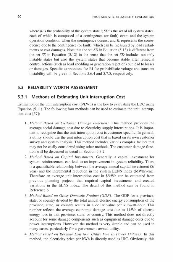
90 PROBABILISTIC RELIABILITY EVALUATION
where p i is the probability of the system state i ; SD is the set of all system states, each of which is composed of a contingence (or fault) event and the system operation condition when the contingence occurs; and R i represents the conse-quence due to the contingence (or fault), which can be measured by load curtail-ments or cost damages. Note that the set SD in Equation (5.13) is different from the set SS in Equation (5.12) in the sense that the set SD includes not only instable states but also the system states that become stable after remedial control actions (such as load shedding or generation rejection) but lead to losses or damages. Specifi c expressions for RI for probabilistic voltage and transient instability will be given in Sections 5.6.4 and 5.7.5 , respectively.
5.3 RELIABILITY WORTH ASSESSMENT
5.3.1 Methods of Estimating Unit Interruption Cost
Estimation of the unit interruption cost ($/kWh) is the key to evaluating the EDC using Equation (5.11) . The following four methods can be used to estimate the unit interrup-tion cost [57] :
1. Method Based on Customer Damage Functions. This method provides the average social damage cost due to electricity supply interruptions. It is impor-tant to recognize that the unit interruption cost is customer - specifi c. In general, a utility should use the unit interruption cost that is based on its own customer survey and system analysis. This method includes various complex factors that may not be easily considered using other methods. The customer damage func-tion will be discussed in detail in Section 5.3.2 .
2. Method Based on Capital Investments. Generally, a capital investment for system reinforcement can lead to an improvement in system reliability. There is a quantifi able relationship between the average annual capital investment ($/year) and the incremental reduction in the system EENS index (MWh/year). Therefore an average unit interruption cost in $/kWh can be estimated from previous planning projects that required capital investments and created variations in the EENS index. The detail of this method can be found in Reference 6.
3. Method Based on Gross Domestic Product ( GDP ) . The GDP for a province, state, or country divided by the total annual electric energy consumption of the province, state, or country results in a dollar value per kilowatt - hour. This number refl ects the average economic damage cost due to 1 kWh of electric energy loss in that province, state, or country. This method does not directly account for some damage components such as equipment damage costs due to power interruptions. However, the method is very simple and can be used in many cases, particularly for a government - owned utility.
4. Method Based on Revenue Lost to a Utility Due To Power Outages. In this method, the electricity price per kWh is directly used as UIC. Obviously, this
c05.indd 90c05.indd 90 1/20/2011 10:25:45 AM1/20/2011 10:25:45 AM
5.3 RELIABILITY WORTH ASSESSMENT 91
method only takes revenue losses of the utility into consideration and can be used in cases where the utility ’ s own benefi ts are focused.
5.3.2 Customer Damage Functions ( CDF s )
5.3.2.1 Customer Survey Approach. Customer damage functions (CDFs) can be obtained by customer surveys. There three basic customer survey approaches:
• Contingent Valuation Approach. A monetary value of power interruption cost is quantifi ed through either the consumer ’ s willingness to pay (WTP) to avoid an interruption, or the willingness to accept (WTA) compensation for an interrup-tion. In general, WTP values are signifi cantly less than WTA values since custom-ers normally object to providing further money for a service for which they consider already paid through an electricity rate. The WTP and WTA values may serve as upper and lower bounds.
• Direct Costing Approach. In this approach, respondents are asked to identify impacts and evaluate the costs associated with particular outage scenarios. The results obtained by this approach are consistent with situations where most losses tend to be tangible, directly identifi able, and quantifi able. The approach is most applicable for industrial and other larger electricity users.
• Indirect Costing Approach. In this approach, respondents are asked questions that relate to the content of their experience. These can include the cost of hypo-thetical insurance to compensate for possible interruption effects, preparatory actions that the respondent may take in the event of interruptions, or consider-ations in ranking a set of reliability/rate alternatives. Evaluations of fi nancial burden that customers would like to bear to alleviate the interruption effects can be obtained through responses to the questions. This approach is most appropriate to cases where customers may lack experience in rating reliability worth, such as residential customers.
5.3.2.2 Establishment of CDF . The establishment of customer damage func-tions includes the following steps:
1. Prepare questionnaires for different customer sectors.
2. Perform a customer survey.
3. Process the data obtained from the customer survey, including fi ltering bad and invalid information using statistical methods.
4. Calculate customer damage functions for individual customer sectors.
5. Calculate composite customer damage functions at different substations, in dif-ferent regions, and for the whole system.
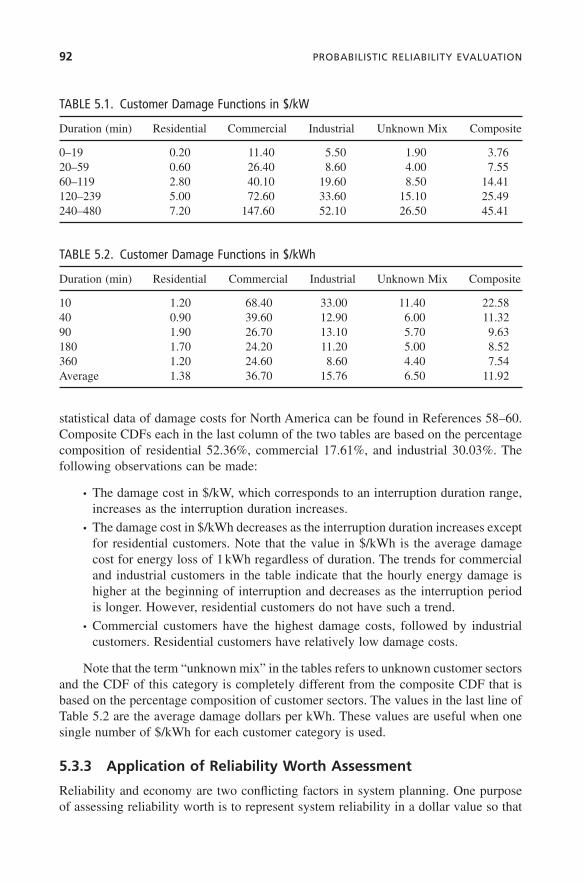
The customer damage function portrays the damage cost as a function of interrup-tion duration. The CDF can be expressed in $/kW or $/kWh. Tables 5.1 and 5.2 provide examples of customer damage functions in $/kW and $/kWh, respectively. More
c05.indd 91c05.indd 91 1/20/2011 10:25:45 AM1/20/2011 10:25:45 AM
92 PROBABILISTIC RELIABILITY EVALUATION
statistical data of damage costs for North America can be found in References 58 – 60. Composite CDFs each in the last column of the two tables are based on the percentage composition of residential 52.36%, commercial 17.61%, and industrial 30.03%. The following observations can be made:
• The damage cost in $/kW, which corresponds to an interruption duration range, increases as the interruption duration increases.
• The damage cost in $/kWh decreases as the interruption duration increases except for residential customers. Note that the value in $/kWh is the average damage cost for energy loss of 1 kWh regardless of duration. The trends for commercial and industrial customers in the table indicate that the hourly energy damage is higher at the beginning of interruption and decreases as the interruption period is longer. However, residential customers do not have such a trend.
• Commercial customers have the highest damage costs, followed by industrial customers. Residential customers have relatively low damage costs.
Note that the term “ unknown mix ” in the tables refers to unknown customer sectors and the CDF of this category is completely different from the composite CDF that is based on the percentage composition of customer sectors. The values in the last line of Table 5.2 are the average damage dollars per kWh. These values are useful when one single number of $/kWh for each customer category is used.
5.3.3 Application of Reliability Worth Assessment
Reliability and economy are two confl icting factors in system planning. One purpose of assessing reliability worth is to represent system reliability in a dollar value so that
TABLE 5.1. Customer Damage Functions in $/kW
Duration (min) Residential Commercial Industrial Unknown Mix Composite
0 – 19 0.20 11.40 5.50 1.90 3.76 20 – 59 0.60 26.40 8.60 4.00 7.55 60 – 119 2.80 40.10 19.60 8.50 14.41 120 – 239 5.00 72.60 33.60 15.10 25.49 240 – 480 7.20 147.60 52.10 26.50 45.41
TABLE 5.2. Customer Damage Functions in $/kWh
Duration (min) Residential Commercial Industrial Unknown Mix Composite
10 1.20 68.40 33.00 11.40 22.58 40 0.90 39.60 12.90 6.00 11.32 90 1.90 26.70 13.10 5.70 9.63 180 1.70 24.20 11.20 5.00 8.52 360 1.20 24.60 8.60 4.40 7.54 Average 1.38 36.70 15.76 6.50 11.92
c05.indd 92c05.indd 92 1/20/2011 10:25:45 AM1/20/2011 10:25:45 AM
5.4 SUBSTATION ADEQUACY EVALUATION 93
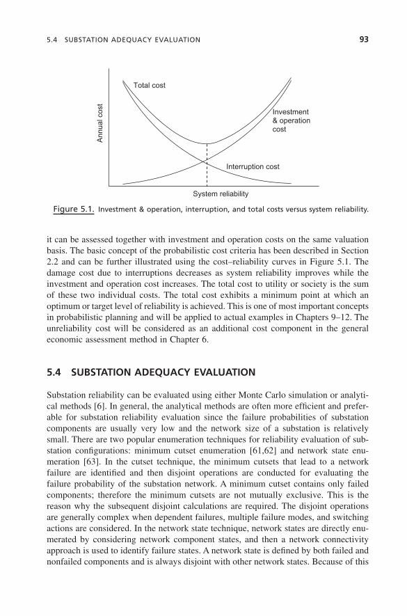
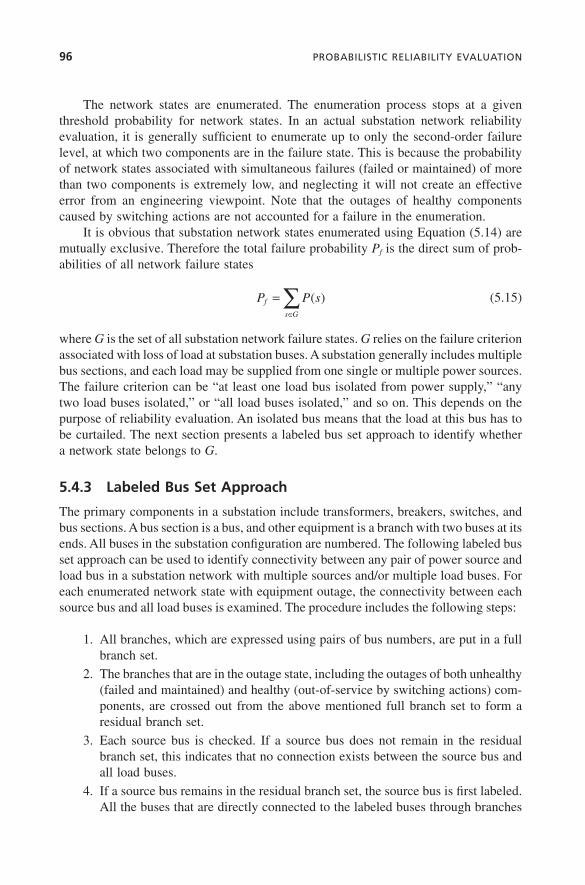
it can be assessed together with investment and operation costs on the same valuation basis. The basic concept of the probabilistic cost criteria has been described in Section 2.2 and can be further illustrated using the cost – reliability curves in Figure 5.1 . The damage cost due to interruptions decreases as system reliability improves while the investment and operation cost increases. The total cost to utility or society is the sum of these two individual costs. The total cost exhibits a minimum point at which an optimum or target level of reliability is achieved. This is one of most important concepts in probabilistic planning and will be applied to actual examples in Chapters 9 – 12 . The unreliability cost will be considered as an additional cost component in the general economic assessment method in Chapter 6 .
5.4 SUBSTATION ADEQUACY EVALUATION
Substation reliability can be evaluated using either Monte Carlo simulation or analyti-cal methods [6] . In general, the analytical methods are often more effi cient and prefer-able for substation reliability evaluation since the failure probabilities of substation components are usually very low and the network size of a substation is relatively small. There are two popular enumeration techniques for reliability evaluation of sub-station confi gurations: minimum cutset enumeration [61,62] and network state enu-meration [63] . In the cutset technique, the minimum cutsets that lead to a network failure are identifi ed and then disjoint operations are conducted for evaluating the failure probability of the substation network. A minimum cutset contains only failed components; therefore the minimum cutsets are not mutually exclusive. This is the reason why the subsequent disjoint calculations are required. The disjoint operations are generally complex when dependent failures, multiple failure modes, and switching actions are considered. In the network state technique, network states are directly enu-merated by considering network component states, and then a network connectivity approach is used to identify failure states. A network state is defi ned by both failed and nonfailed components and is always disjoint with other network states. Because of this
Figure 5.1. Investment & operation, interruption, and total costs versus system reliability.
System reliability
Ann
ual c
ost
Total cost
Investment & operation cost
Interruption cost
c05.indd 93c05.indd 93 1/20/2011 10:25:45 AM1/20/2011 10:25:45 AM
94 PROBABILISTIC RELIABILITY EVALUATION
feature, the network state technique surpasses the minimum cutset technique in dealing with dependent failures between components; multiple failure modes, including short - circuit faults and breaker stuck conditions; and incorporation of breaker switching and protection coordination.
The network state technique is summarized in this section. A simplifi ed minimum cutset technique will be introduced using an actual planning example in Chapter 11 . More materials for substation reliability evaluation can be found in References 6, 10, and 11.
5.4.1 Outage Modes of Components
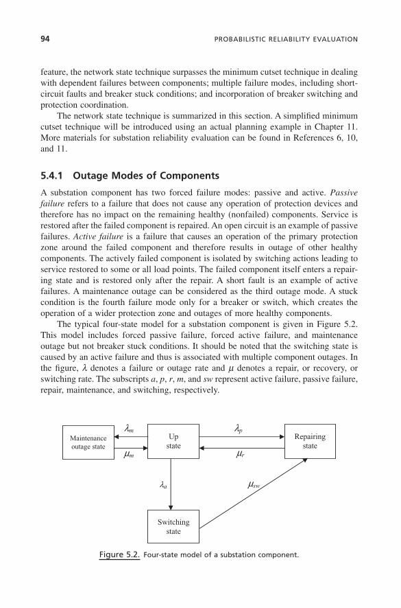
A substation component has two forced failure modes: passive and active. Passive failure refers to a failure that does not cause any operation of protection devices and therefore has no impact on the remaining healthy (nonfailed) components. Service is restored after the failed component is repaired. An open circuit is an example of passive failures. Active failure is a failure that causes an operation of the primary protection zone around the failed component and therefore results in outage of other healthy components. The actively failed component is isolated by switching actions leading to service restored to some or all load points. The failed component itself enters a repair-ing state and is restored only after the repair. A short fault is an example of active failures. A maintenance outage can be considered as the third outage mode. A stuck condition is the fourth failure mode only for a breaker or switch, which creates the operation of a wider protection zone and outages of more healthy components.
The typical four - state model for a substation component is given in Figure 5.2 . This model includes forced passive failure, forced active failure, and maintenance outage but not breaker stuck conditions. It should be noted that the switching state is caused by an active failure and thus is associated with multiple component outages. In the fi gure, λ denotes a failure or outage rate and μ denotes a repair, or recovery, or switching rate. The subscripts a , p , r , m , and sw represent active failure, passive failure, repair, maintenance, and switching, respectively.
Figure 5.2. Four - state model of a substation component.
λm λp
μm μr
λa μsw
Upstate
Repairingstate
Switchingstate
Maintenanceoutage state
c05.indd 94c05.indd 94 1/20/2011 10:25:45 AM1/20/2011 10:25:45 AM
5.4 SUBSTATION ADEQUACY EVALUATION 95
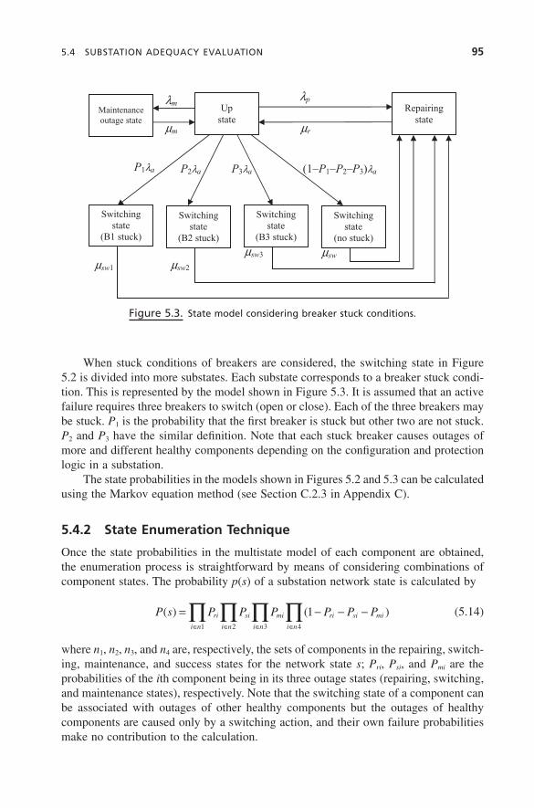
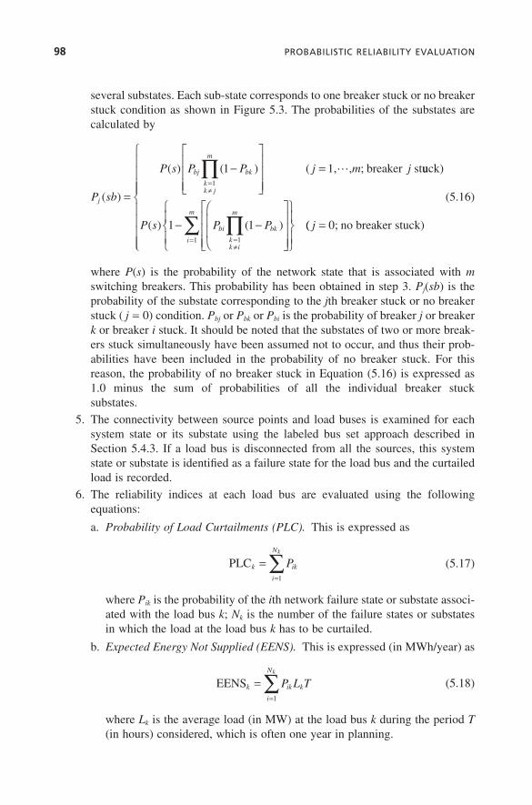
When stuck conditions of breakers are considered, the switching state in Figure 5.2 is divided into more substates. Each substate corresponds to a breaker stuck condi-tion. This is represented by the model shown in Figure 5.3 . It is assumed that an active failure requires three breakers to switch (open or close). Each of the three breakers may be stuck. P 1 is the probability that the fi rst breaker is stuck but other two are not stuck. P 2 and P 3 have the similar defi nition. Note that each stuck breaker causes outages of more and different healthy components depending on the confi guration and protection logic in a substation.
The state probabilities in the models shown in Figures 5.2 and 5.3 can be calculated using the Markov equation method (see Section C.2.3 in Appendix C ).
5.4.2 State Enumeration Technique
Once the state probabilities in the multistate model of each component are obtained, the enumeration process is straightforward by means of considering combinations of component states. The probability p ( s ) of a substation network state is calculated by
P s P P P P P Pri
i n
si
i n
mi
i n
ri si mi
i n
( ) ( )= − − −∈ ∈ ∈ ∈∏ ∏ ∏ ∏
1 2 3 4
1 (5.14)
where n 1 , n 2 , n 3 , and n 4 are, respectively, the sets of components in the repairing, switch-ing, maintenance, and success states for the network state s ; P ri , P si , and P mi are the probabilities of the i th component being in its three outage states (repairing, switching, and maintenance states), respectively. Note that the switching state of a component can be associated with outages of other healthy components but the outages of healthy components are caused only by a switching action, and their own failure probabilities make no contribution to the calculation.
Figure 5.3. State model considering breaker stuck conditions.
λm λp
μm μr
P1λa P2λa P3λa (1–P1–P2–P3)λa
μsw3 μsw μsw1 μsw2
Upstate
Repairingstate
Switchingstate
(B2 stuck)
Maintenanceoutage state
Switchingstate
(B1 stuck)
Switchingstate
(B3 stuck)
Switchingstate
(no stuck)
c05.indd 95c05.indd 95 1/20/2011 10:25:45 AM1/20/2011 10:25:45 AM
96 PROBABILISTIC RELIABILITY EVALUATION
The network states are enumerated. The enumeration process stops at a given threshold probability for network states. In an actual substation network reliability evaluation, it is generally suffi cient to enumerate up to only the second - order failure level, at which two components are in the failure state. This is because the probability of network states associated with simultaneous failures (failed or maintained) of more than two components is extremely low, and neglecting it will not create an effective error from an engineering viewpoint. Note that the outages of healthy components caused by switching actions are not accounted for a failure in the enumeration.
It is obvious that substation network states enumerated using Equation (5.14) are mutually exclusive. Therefore the total failure probability P f is the direct sum of prob-abilities of all network failure states
P P sf
s G
=∈∑ ( ) (5.15)
where G is the set of all substation network failure states. G relies on the failure criterion associated with loss of load at substation buses. A substation generally includes multiple bus sections, and each load may be supplied from one single or multiple power sources. The failure criterion can be “ at least one load bus isolated from power supply, ” “ any two load buses isolated, ” or “ all load buses isolated, ” and so on. This depends on the purpose of reliability evaluation. An isolated bus means that the load at this bus has to be curtailed. The next section presents a labeled bus set approach to identify whether a network state belongs to G .
5.4.3 Labeled Bus Set Approach
The primary components in a substation include transformers, breakers, switches, and bus sections. A bus section is a bus, and other equipment is a branch with two buses at its ends. All buses in the substation confi guration are numbered. The following labeled bus set approach can be used to identify connectivity between any pair of power source and load bus in a substation network with multiple sources and/or multiple load buses. For each enumerated network state with equipment outage, the connectivity between each source bus and all load buses is examined. The procedure includes the following steps:
1. All branches, which are expressed using pairs of bus numbers, are put in a full branch set.
2. The branches that are in the outage state, including the outages of both unhealthy (failed and maintained) and healthy (out - of - service by switching actions) com-ponents, are crossed out from the above mentioned full branch set to form a residual branch set.
3. Each source bus is checked. If a source bus does not remain in the residual branch set, this indicates that no connection exists between the source bus and all load buses.
4. If a source bus remains in the residual branch set, the source bus is fi rst labeled. All the buses that are directly connected to the labeled buses through branches
c05.indd 96c05.indd 96 1/20/2011 10:25:46 AM1/20/2011 10:25:46 AM
5.4 SUBSTATION ADEQUACY EVALUATION 97
can be further labeled using the link information shown in the residual branch set. Starting from the fi rst labeled bus, the labeling process is continued until it can no longer proceed or until all buses are labeled. All the labeled buses form a bus set. If a load bus is not found in the labeled bus set, it does not have a con-nection to the source bus. Otherwise, there is a connection between them. This labeling process is repeated for all the source buses in the residual branch set.
5. The usual failure criterion for a substation confi guration is that if a load bus has been disconnected from all the source buses, this load bus has a failure (load curtailment). A substation network state with at least one load bus failure belongs to the set G .
The labeled bus set approach is running very quickly on a computer since the process of building a residual branch set, labeling buses starting from any source bus, and creat-ing a labeled bus set can be automatically coded in programming. The effects of a protection scheme or switching action, such as the information on which breakers are opened after a short - circuit fault and which breakers are reclosed after isolation of a failed component, can be either automatically identifi ed in a computer program or predefi ned in a data fi le because this is the known information in the protection design of a substation. In other words, the impacts of protection logic and switching can be easily incorporated into the state enumeration technique.
5.4.4 Procedure of Adequacy Evaluation
The reliability evaluation method for a substation confi guration includes the following steps:
1. The four - state model shown in Figure 5.2 can be applied to all substation com-ponents. If the maintenance outage is not considered for a component, the model becomes a three - state representation by deleting the state for maintenance outage. The switching state for each component is individually examined to determine the following:
a. Which healthy components are out of service because of an active failure
b. What switching actions are performed to isolate the failed component in order to transit to the repairing state
c. Which breaker/switch has a possible stuck condition with a probability of occurrence
2. The state space equations of all components are solved using the Markov equa-tion method to obtain the probabilities of each state of the components (see Section C.2.3 in Appendix C ).
3. The state enumeration technique described in Section 5.4.2 is used to select system states. In most cases, considering only fi rst - and second - order failure events is suffi cient.
4. If the breaker stuck conditions are considered, a subenumeration process is performed. A system state associated with breaker switching is divided into
c05.indd 97c05.indd 97 1/20/2011 10:25:46 AM1/20/2011 10:25:46 AM
98 PROBABILISTIC RELIABILITY EVALUATION
several substates. Each sub - state corresponds to one breaker stuck or no breaker stuck condition as shown in Figure 5.3 . The probabilities of the substates are calculated by
P sb
P s P P j m j
j
bj bk
kk j
m
( )
( ) ( )
=
−⎡
⎣
⎢⎢⎢
⎤
⎦
⎥⎥⎥
==≠
∏ 11
( 1, , ; breaker st� uuck)
P s P Pbi bk
kk i
m
i
m
( ) ( )1 111
− −⎛
⎝
⎜⎜
⎡
⎣
⎢⎢⎢
⎤
⎦
⎥⎥⎥
⎧⎨⎪
⎩⎪
⎫⎬⎪
⎭⎪=≠
=∏∑ (( 0; no breaker stuck)j =
⎧
⎨
⎪⎪⎪⎪
⎩
⎪⎪⎪⎪
(5.16)
where P ( s ) is the probability of the network state that is associated with m switching breakers. This probability has been obtained in step 3. P j ( sb ) is the probability of the substate corresponding to the j th breaker stuck or no breaker stuck ( j = 0) condition. P bj or P bk or P bi is the probability of breaker j or breaker k or breaker i stuck. It should be noted that the substates of two or more break-ers stuck simultaneously have been assumed not to occur, and thus their prob-abilities have been included in the probability of no breaker stuck. For this reason, the probability of no breaker stuck in Equation (5.16) is expressed as 1.0 minus the sum of probabilities of all the individual breaker stuck substates.
5. The connectivity between source points and load buses is examined for each system state or its substate using the labeled bus set approach described in Section 5.4.3 . If a load bus is disconnected from all the sources, this system state or substate is identifi ed as a failure state for the load bus and the curtailed load is recorded.
6. The reliability indices at each load bus are evaluated using the following equations:
a. Probability of Load Curtailments ( PLC ) . This is expressed as
PLCk ik
i
N
Pk
==∑
1
(5.17)
where P ik is the probability of the i th network failure state or substate associ-ated with the load bus k ; N k is the number of the failure states or substates in which the load at the load bus k has to be curtailed.
b. Expected Energy Not Supplied ( EENS ) . This is expressed (in MWh/year) as
EENSk ik k
i
N
P L Tk
==∑
1
(5.18)
where L k is the average load (in MW) at the load bus k during the period T (in hours) considered, which is often one year in planning.
c05.indd 98c05.indd 98 1/20/2011 10:25:46 AM1/20/2011 10:25:46 AM
5.5 COMPOSITE SYSTEM ADEQUACY EVALUATION 99
c. Expected Frequency of Load Curtailments ( EFLC ) . This is expressed in the number of failures per year. For each failure state of a load bus, the state frequency can be obtained using the relationship between the state probabil-ity and departure rates:
F Pik ik j
j
Mi
==∑λ
1
(5.19)
Here, F ik is the frequency of the i th failure state associated with the load bus k ; λ j is the departure rate of the j th component in state i , and it can be a failure, repair, switching, maintenance, or recovery rate depending on the status of the component in state i ; and M i is the number of the departure rates in state i . The EFLC index is the cumulative failure frequency, which can be approximately estimated by
EFLCk ik
i
N
Fk
==∑
1
(5.20)
The transition frequencies between failure states should have been deducted from the sum of all failure state frequencies to obtain the accurate EFLC k index. However, these transition frequencies cannot be directly calculated using the state enumeration technique. Ignorance of this deduction in the evaluation is acceptable from an engineering viewpoint as a transition between failure states almost does not take place in a real operation or main-tenance process of substations.
d. Average Duration of Load Curtailments ( ADLC ) . This is expressed (in hours per failure) as
ADLCPLC
EFLCk
k
k
T= ⋅ (5.21)
7. The system reliability indices for a whole substation can be evaluated using the similar equations. Note that the system EENS index is the sum of all bus EENS indices but the system PLC or EFLC index is not the sum of bus PLC or EFLC indices because a network failure state may be associated with simultaneous load curtailments at several buses.
It should be recognized that this enumeration process considered the average load at a load bus for a given time period. If the load curve is modeled using the multistep model, the total index is the sum of products of the index and probability for each individual load level.
5.5 COMPOSITE SYSTEM ADEQUACY EVALUATION
Composite generation and transmission system adequacy evaluation is one of the most important technical activities in probabilistic transmission planning. This is a more
c05.indd 99c05.indd 99 1/20/2011 10:25:46 AM1/20/2011 10:25:46 AM
100 PROBABILISTIC RELIABILITY EVALUATION
complex task compared to substation reliability evaluation. It is associated with the two aspects of system analysis and practical considerations in selecting system states. System analysis is not simple connectivity identifi cation but requires power fl ow calculations, contingency analysis, rescheduling of generations, elimination of system limit violations, and load shedding. Selection of system states involves different con-siderations and various outage models, such as derated states, common cause outages, dependent outages, weather - related failures of transmission lines, bus load uncertainty and correlation, reservoir dispatches, and operating conditions [6,10,25,64 – 76] .
Composite system adequacy evaluation was briefl y summarized in Section 2.3.1 . This section provides more details.
5.5.1 Probabilistic Load Models
The load models used in the composite system reliability evaluation include the fol-lowing three aspects:
• Load curves
• Load uncertainty
• Load correlation
5.5.1.1 Load Curve Models. When the sequential Monte Carlo method is used, a chronological load curve is directly employed. For the state enumeration or state sampling method, a nonchronological load duration curve is utilized. The follow-ing three situations are encountered in practical applications:
• A single - system load curve is considered, and loads at all buses are scaled pro-portionally to follow the shape of the given system load curve. In this case, a multistep model that is similar to that in Figure 3.4 can be created to represent the load duration curve.
• Loads at some buses may remain fl at all the time, such as an industrial customer with the same power demand every hour. It is easy to model the constant loads at certain buses while other bus loads follow a load curve.
• Bus loads are classed into multiple bus groups that follow different load curves. In this case, several load duration curves have to be created, with each curve representing a bus group. The multistep load models have to capture the correla-tion between all the load curves.
The K - mean clustering technique employed to create the multistep load models has been described in Section 3.3.1 .
5.5.1.2 Load Uncertainty Model. The load uncertainty at each load level can be represented using a normally distributed random variable and can be modeled as
M z Mij ij ij ijσ σ= + (5.22)
c05.indd 100c05.indd 100 1/20/2011 10:25:46 AM1/20/2011 10:25:46 AM
5.5 COMPOSITE SYSTEM ADEQUACY EVALUATION 101
where M ij is the i th load level on the j th curve in the multistep load model obtained using the K - mean technique described in Section 3.3.1 , M σ ij is a random sample value around M ij , z ij is the standard normal distribution random variable corresponding to the i th load level on the j th curve, and σ ij is the standard deviation representing the uncer-tainty of M ij .
In the AC power - fl ow - based system analysis, both real and reactive power loads at buses are needed. The sample values of bus reactive loads can be calculated from sample values of real loads and power factors.
5.5.1.3 Load Correlation Model. If the correlation between bus loads is considered, the bus load correlation model described in Section 3.4 can be applied.
5.5.2 Component Outage Models
In general, substation layouts are not modeled in composite system reliability evalua-tion since substation reliability evaluation is performed separately. The main compo-nents in composite system reliability are transmission lines, cables, transformers, capacitors, reactors, and generating units.
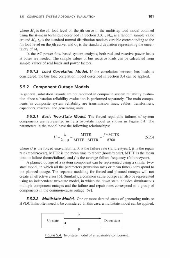
5.5.2.1 Basic Two - State Model. The forced repairable failures of system components are represented using a two - state model as shown in Figure 5.4 . The parameters in the model have the following relationships:
Uf=
+=
+= ∗λ
λ μMTTR
MTTF MTTR
MTTR
8760 (5.23)
where U is the forced unavailability, λ is the failure rate (failures/year), μ is the repair rate (repairs/year), MTTR is the mean time to repair (hours/repair), MTTF is the mean time to failure (hours/failure), and f is the average failure frequency (failures/year).
A planned outage of a system component can be represented using a similar two - state model, in which all the parameters (transition rates or mean times) correspond to the planned outage. The separate modeling for forced and planned outages will not create an effective error [6] . Similarly, a common cause outage can also be represented using an independent two - state model, in which the down state includes simultaneous multiple component outages and the failure and repair rates correspond to a group of components in the common - cause outage [69] .
5.5.2.2 Multistate Model. One or more derated states of generating units or HVDC links often need to be considered. In this case, a multistate model can be applied.
Figure 5.4. Two - state model of a repairable component.
λ
μ
Up state Down state
c05.indd 101c05.indd 101 1/20/2011 10:25:46 AM1/20/2011 10:25:46 AM
102 PROBABILISTIC RELIABILITY EVALUATION
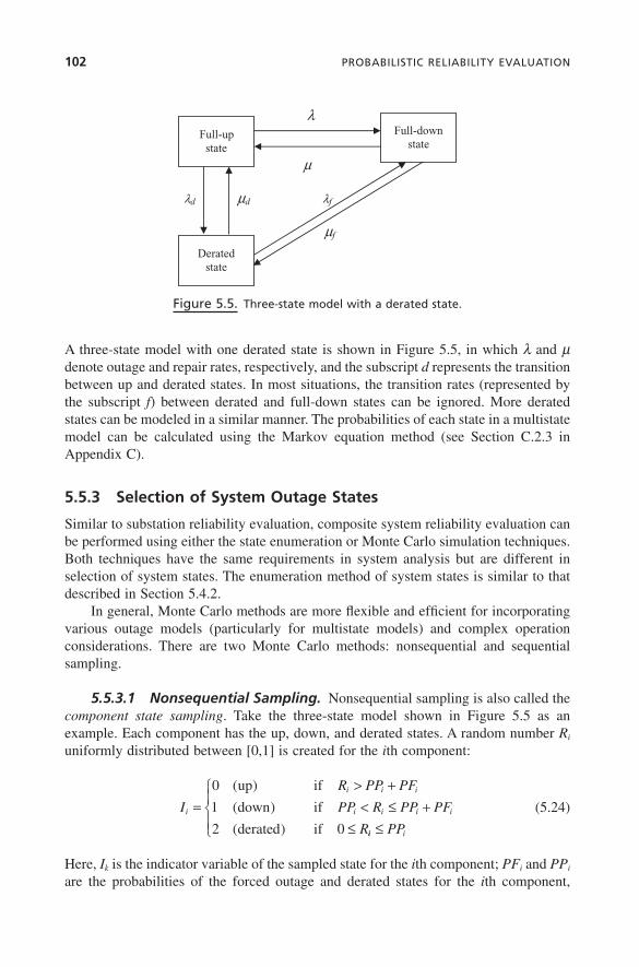
A three - state model with one derated state is shown in Figure 5.5 , in which λ and μ denote outage and repair rates, respectively, and the subscript d represents the transition between up and derated states. In most situations, the transition rates (represented by the subscript f ) between derated and full - down states can be ignored. More derated states can be modeled in a similar manner. The probabilities of each state in a multistate model can be calculated using the Markov equation method (see Section C.2.3 in Appendix C ).
5.5.3 Selection of System Outage States
Similar to substation reliability evaluation, composite system reliability evaluation can be performed using either the state enumeration or Monte Carlo simulation techniques. Both techniques have the same requirements in system analysis but are different in selection of system states. The enumeration method of system states is similar to that described in Section 5.4.2 .
In general, Monte Carlo methods are more fl exible and effi cient for incorporating various outage models (particularly for multistate models) and complex operation considerations. There are two Monte Carlo methods: nonsequential and sequential sampling.
5.5.3.1 Nonsequential Sampling. Nonsequential sampling is also called the component state sampling . Take the three - state model shown in Figure 5.5 as an example. Each component has the up, down, and derated states. A random number R i uniformly distributed between [0,1] is created for the i th component:
I
R PP PF
PP R PP PF
Ri
i i i
i i i i=> +< ≤ +
≤
0
1
2 0
( )
( )
( )
up if
down if
derated if ii iPP≤
⎧⎨⎪
⎩⎪ (5.24)
Here, I k is the indicator variable of the sampled state for the i th component; PF i and PP i are the probabilities of the forced outage and derated states for the i th component,
Figure 5.5. Three - state model with a derated state.
λ
μ
λd μd λf
μf
Full-upstate
Full-downstate
Deratedstate
c05.indd 102c05.indd 102 1/20/2011 10:25:46 AM1/20/2011 10:25:46 AM
5.5 COMPOSITE SYSTEM ADEQUACY EVALUATION 103
respectively. For a two - state model without the derated state, only PF i is needed and PP i is zero. Planned and common - cause outages can be also sampled using separate random numbers. All sampled component states form a system state for the system analysis.
5.5.3.2 Sequential Sampling. The sequential sampling can be classifi ed as either state duration sampling or system state transition sampling [10,77] . State duration sampling consists of the following steps:
1. All components are assumed to be in the up state initially.
2. The duration of each component residing in its present state is sampled. The probability distribution of the state duration should be assumed. For example, the sampling value of the state duration following an exponential distribution is given by
D Rii
i= 1
λln (5.25)
where R i is a uniformly distributed random number between [0,1] corresponding to the i th component. If the present state is the up state, λ i is the outage rate of the i th component; if the present state is the down state, λ i is its repair rate. The methods of generating random variables following different probability distri-butions can be found in Sections A.5.3 and A.5.4 of Appendix A .
3. Step 2 is repeated for all components in the timespan considered (years). The chronological state transition processes of each component in the given times-pan are obtained.
4. The chronological system state transition cycle is obtained by combining the state transition processes of all components.
5.5.4 System Analysis
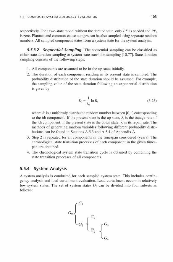
A system analysis is conducted for each sampled system state. This includes contin-gency analysis and load curtailment evaluation. Load curtailment occurs in relatively few system states. The set of system states G 0 can be divided into four subsets as follows:
G0
G1
G1
G2
G2
G4
G3
c05.indd 103c05.indd 103 1/20/2011 10:25:46 AM1/20/2011 10:25:46 AM
104 PROBABILISTIC RELIABILITY EVALUATION
G 1 is the normal state subset without contingency, G1 is the contingency state subset, G 2 is the subset of the contingency states that lead to no system problem, G2 is the subset of the contingency states that create system problems, G 3 is the subset of the contingency states in which system problems can disappear by remedial actions without load curtailment, and G 4 is the subset of the contingency states in which system prob-lems can be resolved only by load curtailments. The subset G 4 here is similar to the set G of substation network failure states in Sections 5.4.2 and 5.4.3 .
For a system state selected by either state enumeration or Monte Carlo simulation method, it is necessary to judge whether it belongs to G1. If so, it is necessary to deter-mine by means of contingency analysis techniques whether it belongs to G2. If so, a remedial action is taken. Only the system states belonging to the subset G 4 make con-tributions to reliability indices.
The contingency analysis includes generating unit outages and transmission com-ponent outages. The analysis for generating unit contingencies is straightforward. If the remaining generation capacity at each generator bus can compensate for the unavailable capacity due to loss of one or more generators at the same bus, no load curtailment is required. Otherwise, generation rescheduling should be performed using the optimiza-tion model that is discussed in the next section.
The transmission contingency analysis is more complex, The purpose is to calcu-late line fl ows and bus voltages following one or more component outages and identify whether there is any overloading, or voltage violation, or isolated bus, or split island. The transmission contingency analysis methods have been discussed in Section 4.6.1 . If the contingency analysis indicates the existence of any system problem, the optimiza-tion model presented in the next section is applied.
5.5.5 Minimum Load Curtailment Model
In any contingency state belonging to G2, either generation outputs at some buses cannot be maintained because of generating unit contingencies or there exist system problems such as branch overloading or voltage violations or system splits due to transmission component outages. For the contingency state, redispatching outputs of generators and reactive power sources and changing transformer turn ratios are needed to maintain the power balance and eliminate the system problems, and at the same time to avoid load curtailments if possible or to minimize the total load curtailment if unavoidable. The following minimization model of load curtailment can be applied for this purpose:
min w Ci i
i
ND
=∑
1
(5.26)
P P C V V G B i NGi Di i i j ij ij ij ij
j
N
− + = + ==∑ ( cos sin ) (δ δ
1
1, , )… (5.27)
Q Q Q CQ
PV V G B iGi Ci Di i
Di
Dii j ij ij ij ij
j
N
+ − + = − ==∑ ( sin cos ) (δ δ
1
1, ,… NN ) (5.28)
c05.indd 104c05.indd 104 1/20/2011 10:25:46 AM1/20/2011 10:25:46 AM
5.5 COMPOSITE SYSTEM ADEQUACY EVALUATION 105
P P P i NGGi Gi Gimin max ( , , )≤ ≤ = 1… (5.29)
Q Q Q i NGGi Gi Gimin max ( , , )≤ ≤ = 1… (5.30)
Q Q Q i NCCi Ci Cimin max ( , , )≤ ≤ = 1… (5.31)
K K K t NTt t tmin max ( , , )≤ ≤ = 1… (5.32)
V V V i Ni i imin max ( , , )≤ ≤ = 1… (5.33)
− ≤ ≤ =T T T l NBl l lmax max ( , , )1… (5.34)
0 1≤ ≤ =C P i NDi Di ( , , )… (5.35)
In these equations P Gi , Q Gi , P Di , Q Di , Q Ci , K t , N , NG , NC , NT , and NB are the same as defi ned in the OPF model in Section 4.4.1 ; C i is the load curtailment variable at load bus i and ND is the number of load buses; and w i is the weighting factor refl ecting importance of loads.
It can be seen that there are the following differences between this minimization model and the OPF model in Section 4.4.1 :
• The bus load curtailment variables are introduced. The reactive loads are cur-tailed proportionally in terms of power factors at each bus. The introduction of load curtailment variables guarantees that the optimization model always has a solution in any outage state.
• The objective function is to minimize the total load curtailment. The values of load curtailment variables are parts of the solution. Nonzero curtailments provide the information needed to calculate reliability indices.
• The weighting factors provide a load curtailment order, which can be automati-cally conducted in the resolution. A greater weighting factor represents a more important bus load.
The minimization model can be solved using the interior point method presented in Section 4.4.2 .
5.5.6 Procedure of Adequacy Evaluation
The adequacy evaluation method for a composite system using the nonsequential Monte Carlo simulation includes the following steps:
1. The state probabilities of system components are calculated using the compo-nent outage models in Section 5.5.2 . If a component is represented by a two - state model, the probabilities of up and down states can be obtained directly from the statistical data. If a component is represented by a multistate model, the state space equation of the model is solved using the Markov equation method to obtain its state probabilities.
2. The multistep load model is created using the method described in Section 3.3.1 . The following state sampling process is performed for each load level.
c05.indd 105c05.indd 105 1/20/2011 10:25:46 AM1/20/2011 10:25:46 AM
106 PROBABILISTIC RELIABILITY EVALUATION
3. A system state is selected using Monte Carlo simulations. This is associated with random determination of bus loads and component states:
a. Load uncertainty and correlation are modeled using the approaches described in Section 5.5.1 .
b. Component states (up, down, or derated) are sampled using the approach described in Section 5.5.3.1 . Note that the forced, planned, and common - cause outages are modeled using independent and separate random variables.
4. A contingency analysis is performed using the method summarized in Section 5.5.4 and detailed in Section 4.6.1 .
5. An optimal power fl ow analysis is conducted using the minimization load cur-tailment model in Section 5.5.5 . If the load curtailment is not zero, the selected state is a failure one. The load curtailments in system failure states are recorded.
6. Steps 3 – 5 are repeated for all system states sampled in the Monte Carlo simula-tions and for all load levels in the multistep load model.
7. The reliability indices for the system or at each bus are calculated using the following equations:
a. Probability of Load Curtailments ( PLC ) . This is expressed as
PLC =⎛
⎝⎜
⎞
⎠⎟
∈=∑∑ n s
N
T
Tis G
i
i
NL
i
( )
41
(5.36)
where n ( s ) is the number of states s occurring in the sampling; N i is the total number of samples at the i th load level in the multistep load model; G 4 i is the set of all system failure states at the i th load level, where the defi nition of G 4 has been given in Section 5.5.4 ; T i is the time length (in hours) of the i th load level; T is the total hours of the load curve considered, which is often one year; and NL is the number of load levels.
b. Expected Energy Not Supplied ( EENS ) . This is expressed (in MWh/year) as
EENS =⎛
⎝⎜
⎞
⎠⎟ ⋅
∈=∑∑ n s C s
NT
is G
i
i
NL
i
( ) ( )
41
(5.37)
where C ( s ) is the load curtailment (in MW) in state s .
c. Expected Frequency of Load Curtailments ( EFLC ) . This is expressed (in failures per year) as
EFLC =⎛
⎝⎜
⎞
⎠⎟
=∈=∑∑∑ n s
N
T
Tij
j
m s
s G
i
i
NL
i
( )( )
λ11 4
(5.38)
where λ j is the j th departure rate of the components in state s ; and m ( s ) is the total number of transition rates departing from state s. As in Equation
c05.indd 106c05.indd 106 1/20/2011 10:25:47 AM1/20/2011 10:25:47 AM
5.6 PROBABILISTIC VOLTAGE STABILITY ASSESSMENT 107
(5.20) , the transition frequencies between failure states have been ignored in Equation (5.38) , leading to an approximate estimation of the frequency index.
d. Average Duration of Load Curtailments ( ADLC ) . This is expressed (in hours per failure) as
ADLC = ⋅PLC T
EFLC (5.39)
There are similar procedures when the state enumeration or sequential sampling tech-niques are used. The system analysis for selected system states is the same for all the techniques; the difference is associated only with selection of system states. If the sequential sampling technique is utilized, the frequency index can be exactly estimated but requires much more efforts in computations. A compromise between the computa-tional cost and the accuracy just for the frequency index should be carefully considered when a simulation method is selected. The formulas for index calculations have varied expressions for the different techniques. More detailed information can be found in References 6 and 10.
5.6 PROBABILISTIC VOLTAGE STABILITY ASSESSMENT
The purpose of probabilistic voltage stability assessment is to evaluate the average voltage instability risk under various contingencies. The voltage stability analysis for a huge number of system contingency states has to be conducted in the assessment. The continuation power fl ow method is very slow and thus inappropriate for this purpose. A new technique, which includes an optimization model, the modal analysis of reduced Jacobian matrix and Monte Carlo simulations, is presented to assess the average voltage instability risk of a transmission system under various outage condi-tions [78] .
The basic idea is as follows. For each contingency state, the optimization model is used to identify insolvability of power fl ow. If there is no power fl ow solution, this may be caused by either system voltage collapse (system instability) or numerical computation instability. Singularity analysis of the reduced Jacobian matrix can be used to differentiate the two cases. If the power fl ow is solvable, the solution obtained from the optimization model may correspond to either the upper portion (stable) or lower portion (instable) of a Q – V curve. The signs of eigenvalues of the reduced Jacobian matrix can be used to distinguish the two cases. Therefore, system voltage instability can be recognized by combining the optimization model and the reduced Jacobian matrix method. Introduction of the optimization model avoids considerable power fl ow calculations in the continuation power fl ow method, which are required to gradually reach the collapse point. The Monte Carlo simulation is used to select system contingency states, from which the average voltage instability risk indices can be assessed.
c05.indd 107c05.indd 107 1/20/2011 10:25:47 AM1/20/2011 10:25:47 AM
108 PROBABILISTIC RELIABILITY EVALUATION
5.6.1 Optimization Model of Recognizing Power Flow Insolvability
In this optimization model, real and reactive powers of generators, reactive power outputs of VAR equipments, turn ratios of transformers, and real power curtailments at load buses are control variables; real and imaginary parts of bus voltages are state variables; and the minimization of total load curtailment is the objective function.
min w Ci i
i
ND
=∑
1
(5.40)
subject to
P P C P P i NGi Di i Lij Tij
ij Sij S TiLi
− + − − = =∈∈∑∑ 0 1( , , )… (5.41)
Q Q Q CQ
PQ Q i NGi Ci Di i
Di
DiLij Tij
ij Sij S TiLi
+ − + − − = =∈∈∑∑ 0 1( , , )… (5.42)
e K e t NTi t m= =( , , )1… (5.43)
f K f t NTi t m= =( , , )1… (5.44)
P P P i NGGi Gi Gimin max ( , , )≤ ≤ = 1… (5.45)
Q Q Q i NGGi Gi Gimin max ( , , )≤ ≤ = 1… (5.46)
Q Q Q i NCCi Ci Cimin max ( , , )≤ ≤ = 1… (5.47)
K K K t NTt t tmin max ( , , )≤ ≤ = 1… (5.48)
0 1≤ ≤ =C P i NDi Di ( , , )… (5.49)
where P Gi , Q Gi , P Di , Q Di , Q Ci , K t , N , NG , NC , and NT are the same as defi ned for the minimum load curtailment model in Section 5.5.5 ; e i and f i are the real and imaginary part variables of voltage at bus i ; C i is load curtailment variable at load bus i and ND is the number of load buses; w i is the weighting factor refl ecting importance of load; P Tij and Q Tij are real and reactive fl ows on branch i – j of a transformer with an on - load tap changer (OLTC) and S Ti is the set of OLTC transformer branches connected to bus i ; and P Lij and Q Lij are real and reactive fl ows on non - OLTC branches (lines and trans-formers without OLTC) and S Li is the set of non - OLTC branches connected to bus i.
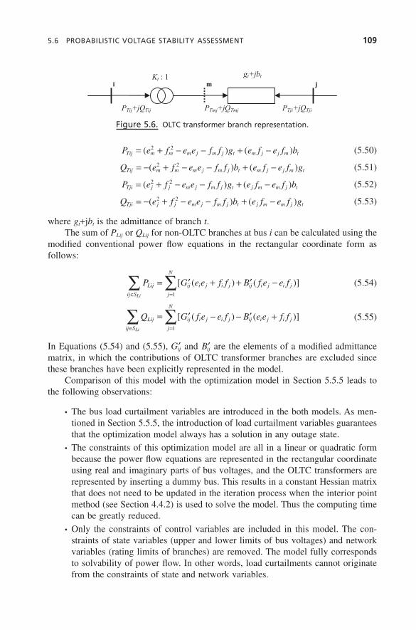
The OLTC transformer branches are modeled using an ideal transformer with a turn ratio as a control variable in series with a regular branch representation. A dummy bus m is added in the middle of each transformer branch t with its two original buses i and j , as shown in Figure 5.6 . In Equations (5.43) and (5.44) , the subscripts i and m are the two end buses of the ideal transformer branch t . If the bus i is located at the high - voltage side, P Tij and Q Tij are calculated using Equations (5.50) and (5.51) ; if the bus i is located at the low - voltage side, P Tji and Q Tji are calculated using Equations (5.52) and (5.53) .
c05.indd 108c05.indd 108 1/20/2011 10:25:47 AM1/20/2011 10:25:47 AM
5.6 PROBABILISTIC VOLTAGE STABILITY ASSESSMENT 109
P e f e e f f g e f e f bTij m m m j m j t m j j m t= + − − + −( ) ( )2 2 (5.50)
Q e f e e f f b e f e f gTij m m m j m j t m j j m t= − + − − + −( ) ( )2 2 (5.51)
P e f e e f f g e f e f bTji j j m j m j t j m m j t= + − − + −( ) ( )2 2 (5.52)
Q e f e e f f b e f e f gTji j j m j m j t j m m j t= − + − − + −( ) ( )2 2 (5.53)
where g t + j b t is the admittance of branch t . The sum of P Lij or Q Lij for non - OLTC branches at bus i can be calculated using the
modifi ed conventional power fl ow equations in the rectangular coordinate form as follows:
P G e e f f B f e e fLij ij i j i j ij i j i j
j
N
ij SLi
= ′ + + ′ −=∈∑∑ [ ( ) ( )]
1
(5.54)
Q G f e e f B e e f fLij ij i j i j ij i j i j
j
N
ij SLi
= ′ − − ′ +=∈∑∑ [ ( ) ( )]
1
(5.55)
In Equations (5.54) and (5.55) , ′Gij and ′Bij are the elements of a modifi ed admittance matrix, in which the contributions of OLTC transformer branches are excluded since these branches have been explicitly represented in the model.
Comparison of this model with the optimization model in Section 5.5.5 leads to the following observations:
• The bus load curtailment variables are introduced in the both models. As men-tioned in Section 5.5.5 , the introduction of load curtailment variables guarantees that the optimization model always has a solution in any outage state.
• The constraints of this optimization model are all in a linear or quadratic form because the power fl ow equations are represented in the rectangular coordinate using real and imaginary parts of bus voltages, and the OLTC transformers are represented by inserting a dummy bus. This results in a constant Hessian matrix that does not need to be updated in the iteration process when the interior point method (see Section 4.4.2 ) is used to solve the model. Thus the computing time can be greatly reduced.
• Only the constraints of control variables are included in this model. The con-straints of state variables (upper and lower limits of bus voltages) and network variables (rating limits of branches) are removed. The model fully corresponds to solvability of power fl ow. In other words, load curtailments cannot originate from the constraints of state and network variables.
Figure 5.6. OLTC transformer branch representation.
i j m
PTij+jQTij PTji+jQTjiPTmj+jQTmj
Kt : 1 gt+jbt
c05.indd 109c05.indd 109 1/20/2011 10:25:47 AM1/20/2011 10:25:47 AM
110 PROBABILISTIC RELIABILITY EVALUATION
The optimization model described above has the following features:
• When the solution of the model does not lead to load curtailment, the correspond-ing power fl ow is solvable and the power fl ow solution has been obtained. When the solution of the model results in any load curtailment, this indicates that the corresponding power fl ow has no solution but the model recovers solvability and provides a critical solution with minimum load curtailment.
• Unlike the continuation power fl ow method, in which many consecutive power fl ow solutions are required to gradually approach the voltage collapse point, the optimization model needs to be solved only once for judging the solvability of power fl ow.
• The model can fl exibly handle the constraints of control variables. Either all control variables are taken into consideration to enhance system voltage stability, or some control variables can be fi xed if necessary. This depends on the opera-tional requirements to be considered.
5.6.2 Method for Identifying Voltage Instability
When the optimization model leads to a solution without load curtailment, it is a solution of corresponding power fl ow equations. In most cases, this solution is voltage - stable. Mathematically, however, it is possible that the solution can be located in the lower portion of a Q – V (or P – V ) curve, which represents voltage instability (uncontrollability). When the optimization model has a solution with minimum load curtailment, this indicates that the corresponding power fl ow does not have a solution since loads have to be curtailed to bring solvability back. The minimum load curtail-ment ensures that the solution obtained from the optimization model is a critical solu-tion. It is generally accepted in the utility ’ s practice that if there is no power fl ow solution, the system is thought to be voltage - instable. The optimization model creates a solution point by only one power fl ow calculation step, at which system voltage instability can be judged.
As discussed in Section 4.7.2 , the signs of eigenvalues of the reduced Jacobian matrix J R can be used to recognize voltage instability. The optimization model directly provides a solution point to which the reduced Jacobian matrix technique can be applied. The method of identifying voltage instability for any contingency state includes the following three steps:
1. The optimization model is solved.
2. If the solution requires load curtailments, the system is thought to have reached the voltage collapse point.
3. If the solution does not require any load curtailment, the eigenvalues of the reduced Jacobian matrix J R at the solution point are calculated. If the minimum eigenvalue is larger than a given positive threshold (a small value close to 0.0), system voltage stability is confi rmed. Otherwise, if at least one eigenvalue is smaller than the threshold, the system is thought to be voltage - unstable.
c05.indd 110c05.indd 110 1/20/2011 10:25:47 AM1/20/2011 10:25:47 AM
5.6 PROBABILISTIC VOLTAGE STABILITY ASSESSMENT 111
In applications, the following modifi cations in step 2 or/and step 3 can be performed:
• Conceptually, a critical solution with minimum load curtailment from the opti-mization model corresponds to the voltage collapse point only when there is no numerical computation instability problem. Unfortunately, the numerical instabil-ity problem, which leads to a false load curtailment case, although rare, may occur. This depends on not only the algorithm but also the coding quality of a computer program. To exclude such a falsehood from the set of voltage instability cases, step 2 can be modifi ed as follows. The eigenvalues of the reduced Jacobian matrix J R at the critical solution with minimum load curtailment are calculated. If the absolute value of at least one eigenvalue is smaller than the threshold, the voltage collapse is confi rmed . Otherwise, if the minimum eigenvalue is larger than the threshold, the false load curtailment is caused by numerical instability but not by voltage collapse. This modifi cation can improve the accuracy of results. However, it should be pointed out that in general, the error due to numeri-cal instability is small as long as the computer program is suffi ciently robust, and this modifi cation may not be needed in many practical cases in order to reduce computational efforts.
• Considerable calculations indicate that generally, if a power fl ow solution is located in the lower portion of a Q – V curve, there must be at least one bus whose voltage is lower than the normally permissible operational voltage limit. Step 3 can be modifi ed as follows. If a solution without load curtailment is obtained from the optimization model, all bus voltages at this solution are checked. If all the bus voltages are within the normal operational limits, the system voltage stability at the solution point is confi rmed. Otherwise, if there is at least one bus whose voltage is lower than the normal voltage level, the reduced Jacobian matrix method described in step 3 is applied. This modifi cation can signifi cantly reduce computational efforts since fi nding the eigenvalues of J R is a time - consuming process and the majority of contingency cases will not cause voltage instability. Strictly speaking, this alternative approach may introduce a very small risk of misjudgment and should be used with caution for real - time voltage stability assessment. However, it is suffi ciently accurate and acceptable for calculating the probabilistic voltage instability risk indices for planning purposes.
5.6.3 Determination of Contingency System States
In the probabilistic voltage stability risk assessment, various contingency system states are randomly sampled. Determination of contingency system states includes
• Selection of precontingency system states (network topology, generation capaci-ties, and bus loads)
• Selection of contingencies
5.6.3.1 Selection of Precontingency System States. The system compo-nents (transmission components and generating units) are divided into two groups:
c05.indd 111c05.indd 111 1/20/2011 10:25:47 AM1/20/2011 10:25:47 AM
112 PROBABILISTIC RELIABILITY EVALUATION
crucial component set and noncrucial component set. A failure event of components in the crucial set may cause voltage instability, whereas a failure event of components in the noncrucial set does not cause voltage instability. This division can be determined from the knowledge and experience of engineers on an actual system. A conservative division is always used. If we are uncertain about a component, it is assigned to the crucial set. The unavailability due to forced failures of the components in the crucial set is not taken into consideration in selecting a precontingency system state since their forced failures will be considered as random contingencies later. The unavailability due to both forced failures and planned outages of components in the non - crucial set and the unavailability due to only planned outages of components in the crucial set make contributions to the probability of a precontingency system state. The precontingency state must be a stable one. A Monte Carlo sampling method similar to that described in Section 5.5.3.1 , or an enumeration technique is used to select precontingency system states.
Voltage stability is sensitive to load profi les. The real power load at a bus can be assumed to follow a normal distribution, whereas its reactive load is assumed to have a change proportional to the random variation of the real load with a constant power factor. A standard normally distributed random number x i for the real load at the i th bus is created using the method in Section A.5.4.2 of Appendix A . The bus loads are cal-culated by
P x PDi i i Di= +σ mean (5.56)
Q PQ
PDi Di
Di
Di
=mean
mean (5.57)
where PDimean and QDi
mean are the mean values of real and reactive loads at the i th bus; P Di and Q Di are their sampled values, which are used in the optimization model; x i is a stan-dard normal distribution random variable; and σi is the standard deviation of PDi
mean. Obviously, the load model is the same as that in Section 5.5.1.2 . Besides, the
methods for load curve modeling in Section 5.5.1.1 and load correlation modeling in Section 5.5.1.3 can be also applied if necessary.
5.6.3.2 Selection of Contingencies. A forced failure (fault event) of com-ponents in the crucial set leads to a contingency. Such a forced failure can occur when these components are in service (not in a planned outage). The status as to whether a component is in planned outage has been randomly determined in selecting the precon-tingency system state. Selection of contingencies depends on the forced failure prob-ability of the components. It should be noted that this probability is not the forced unavailability of components given in Equation (5.23) , which is calculated by both failure and repair rates. In the probabilistic voltage stability assessment, we are con-cerned about only occurrence of a forced failure event but not a subsequent repair (or recovery) process because as long as it occurs, the system may lose voltage stability in a very short time, which has nothing to do with repairing. The probability of occurrence of a contingency event can be estimated using the Poisson distribution with a constant
c05.indd 112c05.indd 112 1/20/2011 10:25:47 AM1/20/2011 10:25:47 AM
5.6 PROBABILISTIC VOLTAGE STABILITY ASSESSMENT 113
occurrence rate. Using the Poisson distribution formula, the probability of no contin-gency occurring in the time period t is given by
Pe t
eno
to t
oo= =
−−
λλλ( )0
0! (5.58)
where P no is the probability of no contingency occurrence, λ o is the average occurrence rate of a contingency, and t is the duration considered.
The probability of a failure or contingency occurring in t is
P eoto= − −1 λ (5.59)
Obviously, Equation (5.59) is simply an occurrence probability following the exponential distribution. In fact, the Poisson and exponential distributions are essen-tially consistent since both are based on the constant rate assumption. Equation (5.59) is applied to all the components in the crucial set. Each component has a different average contingency occurrence rate, which can be calculated from historical fault records.
5.6.4 Assessing Average Voltage Instability Risk
The procedure of assessing voltage instability risk using the Monte Carlo simulation includes the following steps:
1. Precontingency system states are selected using the Monte Carlo simulation methods described in Section 5.6.3.1 . As mentioned earlier, the forced unavail-ability of components in the crucial set is excluded in selection of precontin-gency system states.
2. Contingencies (forced failures) of the components in the crucial set that are not in a planned outage status during the selection of precontingency system states are randomly determined. A uniformly distributed random number R in the interval [0,1] is created for each component or component group (simultaneous multiple component failures) in the crucial set. If R < P o , the contingency occurs; otherwise the contingency does not occur.
3. The optimization model in Section 5.6.1 is used to create a solution point for the selected contingency, which is either a solution without load curtailment or a critical solution with minimum load curtailment.
4. The reduced Jacobian matrix method outlined in Section 5.6.2 and detailed in Section 4.7.2 is used to judge whether each of the sampled contingency states is voltage - stable.
5. The following two voltage instability risk indices are calculated:
PVI = m
M (5.60)
c05.indd 113c05.indd 113 1/20/2011 10:25:47 AM1/20/2011 10:25:47 AM
114 PROBABILISTIC RELIABILITY EVALUATION
ELCAVI ===∑∑ C
Mij
i
N
j
M j
11
(5.61)
where PVI is the probability of voltage instability, ELCAVI is the expected load curtailment to avoid voltage instability, m is the number of system states that are voltage - unstable, M is the total number of sampled system states, C ij is the load curtailment at the i th bus in the j th sampled system state, and N j is the number of buses in the j th system state. Note that the number of buses may be changed since isolated buses may occur as a result of branch outages in a sampled system state. The PVI index represents the average likelihood of voltage instability occurring in various contingencies. The ELCAVI index rep-resents the average load curtailments required to prevent voltage instability in various contingencies. The load curtailments at isolated buses are not included in the ELCAVI index, as these are not considered as consequences to avoid system voltage instability.
6. Steps 1 – 5 are repeated until a variance coeffi cient of the PVI or ELCAVI index is smaller than a specifi ed threshold.
The voltage instability risk indices can be used as system performance indicators in transmission planning along with other adequacy indices. For instance, an acceptable PVI index target may be established after considerable studies for a system are con-ducted. If the PVI index for a future year in planning is higher than the target, this indicates that the voltage stability performance of the system has deteriorated and some reinforcement is needed. The difference in the PVI or ELCAVI index before and after a reinforcement project represents the improvement in system voltage stability due to the project.
5.7 PROBABILISTIC TRANSIENT STABILITY ASSESSMENT
The purpose of probabilistic transient stability assessment in transmission planning is to evaluate the average transient instability risk under various fault events. Similar to the probabilistic voltage stability assessment, the probabilistic transient stability assess-ment needs to evaluate both probabilities and consequences of a huge number of fault events. The probability and consequence of a fault depend on multiple factors, including prefault system conditions, fault location and types, protection schemes, and distur-bance sequences [79,80] . The consequence evaluation requires the simulation of tran-sient stability and impact analysis. The Monte Carlo simulation method for probabilistic transient stability assessment is discussed in this section.
5.7.1 Selection of Prefault System States
Selection of prefault system states in the probabilistic transient stability assessment is similar to that in the probabilistic voltage stability assessment. The state sampling
c05.indd 114c05.indd 114 1/20/2011 10:25:47 AM1/20/2011 10:25:47 AM
5.7 PROBABILISTIC TRANSIENT STABILITY ASSESSMENT 115
method for generation and transmission components in Section 5.5.3.1 is used to deter-mine network topology and available generation capacities in prefault system states. As mentioned in Section 5.6.3.1 , it is important to appreciate that the unavailability of forced failures of the components in the crucial set is excluded in calculating the prob-ability of a prefault system state since these failures are the fault events but not a portion of a prefault state. The modeling methods for load curves and bus load uncertainty and correction in Section 5.5.1 are used to select bus load states.
5.7.2 Fault Probability Models
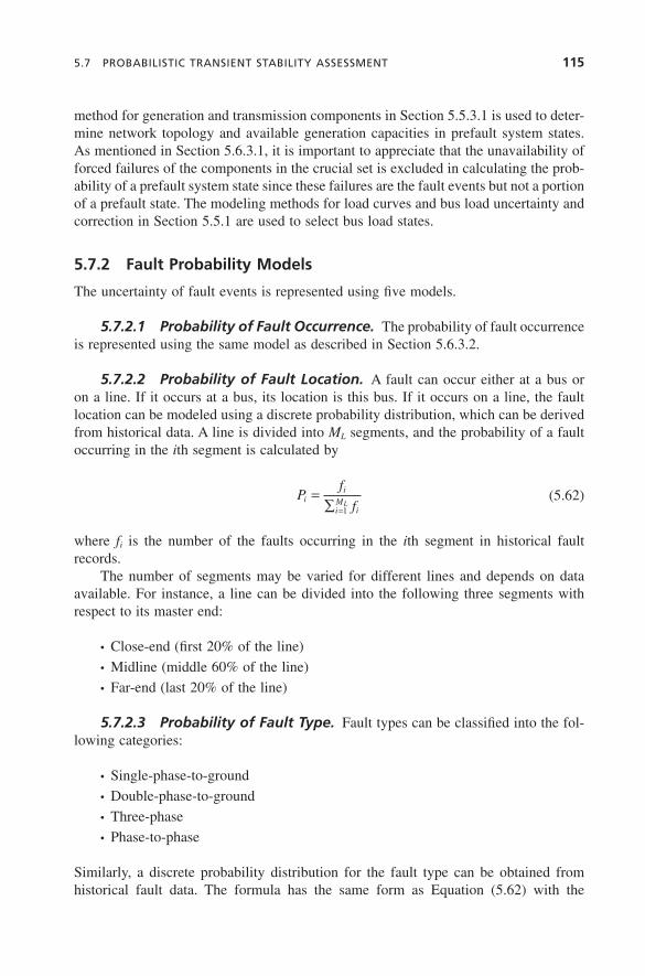
The uncertainty of fault events is represented using fi ve models.
5.7.2.1 Probability of Fault Occurrence. The probability of fault occurrence is represented using the same model as described in Section 5.6.3.2 .
5.7.2.2 Probability of Fault Location. A fault can occur either at a bus or on a line. If it occurs at a bus, its location is this bus. If it occurs on a line, the fault location can be modeled using a discrete probability distribution, which can be derived from historical data. A line is divided into M L segments, and the probability of a fault occurring in the i th segment is calculated by
Pf
fi
i
iM
iL
=∑ =1
(5.62)
where f i is the number of the faults occurring in the i th segment in historical fault records.
The number of segments may be varied for different lines and depends on data available. For instance, a line can be divided into the following three segments with respect to its master end:
• Close - end (fi rst 20% of the line)
• Midline (middle 60% of the line)
• Far - end (last 20% of the line)
5.7.2.3 Probability of Fault Type. Fault types can be classifi ed into the fol-lowing categories:
• Single - phase - to - ground
• Double - phase - to - ground
• Three - phase
• Phase - to - phase
Similarly, a discrete probability distribution for the fault type can be obtained from historical fault data. The formula has the same form as Equation (5.62) with the
c05.indd 115c05.indd 115 1/20/2011 10:25:47 AM1/20/2011 10:25:47 AM
116 PROBABILISTIC RELIABILITY EVALUATION
following defi nition changes: P i is the probability of the i th fault type, f i is the number of the i th fault type, and M L = 4.
5.7.2.4 Probability of Unsuccessful Automatic Reclosure. Most high - voltage overhead lines are equipped with automatic reclosure devices. A “ false ” fault will not create any severe consequence if the automatic reclosure is successful. The second fault clearing is needed only when the automatic reclosure fails. Conceptually, the probability of unsuccessful automatic reclosure may be obtained from historical data. However, many data collection systems do not record the information on the rela-tive success of reclosure but do provide a description of the cause of faults. Generally, there is a strong correlation between the cause of faults and the probability of successful automatic reclosure. For instance, a typical statistic analysis indicates that the automatic reclosure is successful for over 90% of the faults caused by lightning but for only about 50% of the faults due to other causes. The probability of unsuccessful automatic reclo-sure can be estimated using the conditional probability concept:
P P L P U L P O P U Oru = +( ) ( ) ( ) ( )| | (5.63)
where P ru is the probability of unsuccessful automatic reclosure; P ( L ) and P ( O ) are the probabilities of faults, respectively, due to lightning and other causes, which can be easily obtained from historical records; and P ( U | L ) and P ( U | O ) are the conditional probabilities of unsuccessful reclosure given that the fault is caused by lightning and other causes, respectively, which can be estimated through a statistic analysis. The equation can be extended to distinguish more fault causes if there are suffi cient data records.
5.7.2.5 Probability of Fault Clearing Time. The process of clearing a fault is composed of three tasks: fault detection, relay operation, and breaker operation. The fault detection can be assumed to be completed instantly. The times of relay and breaker operations are both random. There are two modeling approaches for the fault clearing time:
• The relay and breaker operation times are modeled using two separate probability distributions, and the probability distribution of the total fault clearing time is obtained by a convolution.
• The total fault clearing time is assumed to directly follow a probability distribution.
Generally, a normal distribution assumption is used for the relay or breaker operation time, or the total fault clearing time. The estimates of the mean and standard deviation for the normal distribution can be determined from historical data. A system loses transient stability only when the fault clearing time is longer than the critical clearing time.
c05.indd 116c05.indd 116 1/20/2011 10:25:47 AM1/20/2011 10:25:47 AM
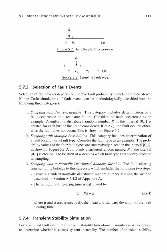
5.7 PROBABILISTIC TRANSIENT STABILITY ASSESSMENT 117
5.7.3 Selection of Fault Events
Selection of fault events depends on the fi ve fault probability models described above. Monte Carlo simulations of fault events can be methodologically classifi ed into the following three categories:
1. Sampling with Two Possibilities. This category includes determination of a fault occurrence or a reclosure failure. Consider the fault occurrence as an example. A uniformly distributed random number R in the interval [0,1] is created for each bus or line to be considered. If R < P o , the fault occurs; other-wise the fault does not occur. This is shown in Figure 5.7 .
2. Sampling with Multiple Possibilities. This category includes determination of a fault location or a fault type. Consider the fault type as an example. The prob-ability values of the four fault types are successively placed in the interval [0,1], as shown in Figure 5.8 . A uniformly distributed random number R in the interval [0,1] is created. The location of R denotes which fault type is randomly selected in sampling.
3. Sampling with a Normally Distributed Random Variable. The fault clearing time sampling belongs to this category, which includes the following two steps:
• Create a standard normally distributed random number X using the method described in Section A.5.4.2 of Appendix A .
• The random fault clearing time is calculated by
τ σ μc X= + (5.64)
where μ and σ are, respectively, the mean and standard deviation of the fault clearing time.
5.7.4 Transient Stability Simulation
For a sampled fault event, the transient stability time - domain simulation is performed to determine whether it causes system instability. The number of transient stability
Figure 5.7. Sampling fault occurrence.
R
0 Po 1.0
Figure 5.8. Sampling fault type.
R
0 P1 P2 P3 P4 1.0
c05.indd 117c05.indd 117 1/20/2011 10:25:47 AM1/20/2011 10:25:47 AM
118 PROBABILISTIC RELIABILITY EVALUATION
simulations is very large in the probabilistic transient stability assessment since prefault system states and fault events are randomly selected. The simulation methods have been briefl y described in Section 4.8 . In fact, commercial programs for transient stability can be used. Considerable techniques have been developed to speed up the simulation process, such as the variable step algorithm for differential equations, early termination criteria, and second kick method.
It is important to appreciate that a disturbance sequence must be specifi ed in the transient stability simulation. The disturbance sequence is varied for different fault events and is usually defi ned in operation criteria of a control center. Various special protection systems (SPSs) are installed in many utility systems. These include a variety of remedial action schemes (RASs) such as the generation rejection, switching of VAR equipment, line tripping, and load shedding. Any remedial actions should be also defi ned in the disturbance sequence.
5.7.5 Assessing Average Transient Instability Risk
The procedure of assessing transient instability risk using the Monte Carlo simulation includes the following steps:
1. Prefault system states are selected using the Monte Carlo simulation methods described in Section 5.7.1 . This includes the determination of network topology, generation unit states, and bus loads.
2. Fault events are randomly selected using the Monte Carlo simulation methods described in Section 5.7.3 . This includes the determination of occurrence, loca-tion, and types of faults; successfulness of automatic reclosure; and fault clear-ing time. Note that only those lines and generating units in the crucial set that are not in a planned outage status during selection of prefault system states are considered in selecting occurrence of faults. See Section 5.6.3.1 for the concept of the crucial set.
3. A disturbance sequence in transient stability simulation is specifi ed for each fault. If a special protection system (SPS) is installed for a fault, the remedial actions defi ned in the SPS are included in the disturbance sequence.
4. A time - domain transient stability simulation is performed for each fault event.
5. A consequence analysis is conducted for each fault event. This is the evaluation of damage costs due to transient instability or remedial actions and is associated with the following aspects:
• Consequence of system instability
• Load shedding
• Generation rejections
• Equipment damages due to transient overvoltage
• Transfer limit reduction that may lead to losses of revenue
• Penalties for violation on criteria or agreements
c05.indd 118c05.indd 118 1/20/2011 10:25:47 AM1/20/2011 10:25:47 AM
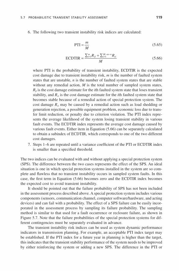
5.7 PROBABILISTIC TRANSIENT STABILITY ASSESSMENT 119
6. The following two transient instability risk indices are calculated:
PTI = m
M (5.65)
ECDTIR =∑ + ∑= =
− −im
fi iM m n
siR R
M1 1 (5.66)
where PTI is the probability of transient instability, ECDTIR is the expected cost damage due to transient instability risk, m is the number of faulted system states that are unstable, n is the number of faulted system states that are stable without any remedial action, M is the total number of sampled system states, R fi is the cost damage estimate for the i th faulted system state that loses transient stability, and R si is the cost damage estimate for the i th faulted system state that becomes stable because of a remedial action of special protection system. The cost damage R si may be caused by a remedial action such as load shedding or generation rejection, a possible equipment problem, economic loss due to trans-fer limit reduction, or penalty due to criterion violation. The PTI index repre-sents the average likelihood of the system losing transient stability in various fault events. The ECDTIR index represents the average cost damage caused by various fault events. Either item in Equation (5.66) can be separately calculated to obtain a subindex of ECDTIR, which corresponds to one of the two different cost damages.
7. Steps 1 – 6 are repeated until a variance coeffi cient of the PTI or ECDTIR index is smaller than a specifi ed threshold.
The two indices can be evaluated with and without applying a special protection system (SPS). The difference between the two cases represents the effect of the SPS. An ideal situation is one in which special protection systems installed in the system are so com-plete and fl awless that no transient instability occurs in sampled system faults. In this case, the fi rst term in Equation (5.66) becomes zero and the ECDTIR index becomes the expected cost to avoid transient instability.
It should be pointed out that the failure probability of SPS has not been included in the assessment process described above. A special protection system includes various components (sensors, communication channel, computer software/hardware, and acting devices) and can fail with a probability. The effect of a SPS failure can be easily incor-porated in the assessment process by sampling its failure probability. The sampling method is similar to that used for a fault occurrence or reclosure failure, as shown in Figure 5.7 . Note that the failure probabilities of the special protection systems for dif-ferent contingencies must be separately evaluated in advance.
The transient instability risk indices can be used as system dynamic performance indicators in transmission planning. For example, an acceptable PTI index target may be established. If the PTI index for a future year in planning is higher than the target, this indicates that the transient stability performance of the system needs to be improved by either reinforcing the system or adding a new SPS. The difference in the PTI or
c05.indd 119c05.indd 119 1/20/2011 10:25:47 AM1/20/2011 10:25:47 AM
120 PROBABILISTIC RELIABILITY EVALUATION
ECDTIR index before and after a reinforcement or SPS project represents the improve-ment of system transient stability due to the project.
5.8 CONCLUSIONS
This chapter discussed the probabilistic reliability evaluation in transmission planning. Reliability of transmission systems includes adequacy and security. Adequacy refl ects the static ability of the system to deliver power and energy from sources to load buses and is associated with network connectivity and power fl ow constraints. Security relates the ability of the system in response to dynamic disturbances and is associated with voltage and transient stability.
Reliability indices are the outcome of quantifi ed reliability evaluation and represent the system risk level. The basic defi nitions of adequacy and security indices are given. It should be appreciated that the defi nitions provide only the general concepts of the indices. The reliability indices have concrete expressions when different evaluation techniques are used.
Reliability worth assessment provides a reliability measure in a monetary value. This is extremely important and useful in the economic analysis of planning projects as it places system reliability on a scale comparable with those of other economic components. The basic idea is to assess the unreliability costs using the unit interruption cost times the EENS index. The four approaches for estimating the unit interruption cost have been described, in which the customer damage function approach is the most poplar one. It should be noted that this is not a unique idea. For example, it has been pointed out in Section 5.7.5 that the unreliability costs can include those due to equip-ment damage, transfer limit reduction, and penalty.
Substation adequacy evaluation, composite generation – transmission adequacy evaluation, and probabilistic voltage and transient stability assessments are illustrated in detail. There are two fundamental reliability evaluation techniques: Monte Carlo simulation and state enumeration. The Monte Carlo methods have been used in com-posite system adequacy evaluation and probabilistic voltage and transient stability assessments, whereas the state enumeration method has been used in substation reli-ability evaluation. Undoubtedly, the Monte Carlo methods can also be applied to sub-station reliability evaluation, and the state enumeration methods can also be utilized in composite system evaluation. More materials can be found in References 6 and 10.
The common feature in probabilistic adequacy and security assessments is evalu-ation of both probabilities and consequences, although there are varied characteristics in different cases. In the substation adequacy evaluation, the component failure models are relatively complicated, particularly when breaker stuck conditions are considered. However, system analysis for the substation adequacy evaluation is straightforward since it is associated only with network connectivity identifi cation. In composite system adequacy evaluation, the component failure models can be simplifi ed, but the conse-quence assessment requires system contingency analyses and the optimization model for load curtailments. In probabilistic voltage and transient stability assessments, the determination of system states includes selections of precontingency states and
c05.indd 120c05.indd 120 1/20/2011 10:25:47 AM1/20/2011 10:25:47 AM

5.8 CONCLUSIONS 121
contingencies or faults. The selection techniques of precontingency states are similar to those used in the composite system adequacy evaluation, whereas the selection of contingencies or faults depends on their probability models. A technique of combining the optimization model with the reduced Jacobian matrix method has been developed to recognize power fl ow solvability and to identify voltage instability. This technique can avoid the calculations of a sequence of power fl ow solutions for gradually approach-ing the collapse point, which are imperative in the continuation power fl ow method. Special protection systems (SPSs) or remedial - action schemes (RASs) are often used for mitigating or eliminating system instability. Including or excluding SPS in the probabilistic transient stability assessment will have very different effects on the insta-bility risk indices. It should be also emphasized that a SPS is fault - specifi c and can fail itself.
Reliability evaluation is one of the most crucial steps in probabilistic transmission planning. More developments associated with reliability evaluation will be discussed further in the subsequent chapters for actual planning applications.
c05.indd 121c05.indd 121 1/20/2011 10:25:47 AM1/20/2011 10:25:47 AM