Probabilistic Transmission System Planning (Li/Transmission System Planning) || Economic Analysis Methods

123

6.1 INTRODUCTION

Economic analysis and reliability evaluation are two essential aspects in transmission planning. Probabilistic reliability evaluation has been discussed in Chapter 5 . A number of references in engineering economics are available [81 – 84] . The intent of this chapter is to review the useful concepts of engineering economics, to extend them to applica-tions in transmission planning, and particularly to incorporate unreliability costs in overall economic analysis models. This incorporation is a distinguishing feature for probabilistic transmission planning.

As mentioned in Chapter 2 , there are three cost components in a transmission planning project: capital investment, operation cost, and unreliability cost. The compo-sition of capital investment and operation cost, and the basic nature of unreliability cost in the economic analysis are outlined in Section 6.2 . One of the most important concepts in engineering economics is the time value of money. Various costs are comparable only when they are valued at the same point of time. This concept is applicable for all the three cost components. The time value of money and the present value method are illustrated in Section 6.3 . Depreciation is another important concept associated with economic analysis of capital investment and is discussed in Section 6.4 . Economic

6

ECONOMIC ANALYSIS METHODS

Probabilistic Transmission System Planning, by Wenyuan LiCopyright © 2011 Institute of Electrical and Electronics Engineers

c06.indd 123c06.indd 123 1/20/2011 10:26:03 AM1/20/2011 10:26:03 AM

124 ECONOMIC ANALYSIS METHODS

assessment of investment projects is the fundamental analysis in selection and justifi ca-tion of portfolios or alternatives of a project and is addressed in Section 6.5 . Retirement of equipment has signifi cant impacts on system reliability, and therefore a decision on equipment replacement often requires system planning studies. Economic analysis of equipment replacement is discussed in Section 6.6 . The uncertainties of parameters in economic analysis are the origin of fi nancial risks. The probabilistic analysis method used to deal with uncertain factors in the economic analysis is explained in Section 6.7 .

6.2 COST COMPONENTS OF PROJECTS

6.2.1 Capital Investment Cost

The capital investment of a project includes the following subcomponents:

1. Direct Capital Costs. These costs include

• Equipment costs.

• Costs for transportation, installation, and commissioning of equipment.

• Land and right - of - way costs.

• Removal costs of existing facilities.

• Outsource costs for design and other services.

• Contingency costs (unexpected costs).

• Salvage values — these are negative costs if previous facilities have the resid-ual values that can be utilized in a new project.

2. Corporate Overhead. This cost can be expressed as a percentage of total direct capital cost. It represents an allocation of additional corporate costs among capital projects, which are not included in the total direct capital cost.

3. Financial Cost. These costs consist of

• Interest during Construction (IDC). The IDC refl ects the cost of borrowing to fi nance the project for the period during which expenditures are made on the project before it is in service. This cost is also expressed in a percentage of the total direct capital cost. If the period during construction is included in the cash fl ow for present value calculation, it should be excluded from the estimate here to avoid a double count.

• Purchase and Service Taxes (PST). The PST is the government ’ s taxes on pur-chase of equipment and services, which is a percentage of the purchase price.

6.2.2 Operation Cost

The operation cost is estimated on an annual basis and includes the following subcomponents:

1. Operation, Maintenance, and Administration (OMA) Cost. The annual operat-ing cost includes incremental system operation expenditures due to the project. A project may increase or reduce system operation expenditures. If increased,

c06.indd 124c06.indd 124 1/20/2011 10:26:03 AM1/20/2011 10:26:03 AM

6.3 TIME VALUE OF MONEY AND PRESENT VALUE METHOD 125

it is a cost; if reduced, it is a negative cost or benefi t. The annual maintenance cost refers to the yearly expenditure that will be made over the lifecycle of equipment, including repairs, overhauls, replacements of parts, and decommis-sioning. The annual administration cost is general administrative expenses.

2. Taxes. Annual taxes may include property and income taxes. Calculation of property taxes is often based on a percentage of the book value (a capital cost after depreciation) or a market value. Income taxes refer to those taxes charged to the project, such as sales tax. It should be noted that the taxes vary for dif-ferent countries or provinces depending on their tax policies.

3. Network Losses. Some alternatives of a transmission project may either reduce or increase network losses. In the case of reduction, reduced losses can be treated as negative costs or benefi ts. The reduction or increase in network losses includes two implications: (1) it represents the reduction or increase of generation capacity (MW) requirement; (2) it also represents the reduction or increase of energy consumption (MWh). Utilities provide two unit values for network losses: dollars per MW and dollars per MWh. Accordingly, both elements should be included in calculating the cost due to loss increase or the benefi t due to loss reduction. It should be emphasized that the allocation of the cost or benefi t associated with network losses between a utility and its customers is a complex problem under the deregulated power market environment. This depends on the market model. The loss - related cost or benefi t should be allocated or assigned with caution.

6.2.3 Unreliability Cost

The unreliability cost represents the damage cost caused by system component outages (or faults). This cost is the result of probabilistic reliability worth assessment, and its basic concept has been discussed in Chapter 5 . It should be emphasized that the unreli-ability cost due to equipment is an incremental cost and its calculation method is varied in different cases. For example, the unreliability cost due to an equipment addition is the difference in the total system unreliability cost between the two cases with and without the addition, whereas that due to an equipment replacement is the difference in the total system unreliability cost between the two cases with old and new equipment. Note that an equipment addition or replacement generally leads to reduction of system unreliability cost, and therefore the unreliability cost due to equipment addition or replacement is usually a negative cost (benefi t).

6.3 TIME VALUE OF MONEY AND PRESENT VALUE METHOD

More details of these topics can be found in general textbooks of engineering econom-ics [81] .

6.3.1 Discount Rate

The value of money varies over time. This concept is called the time value of money . If one borrows money from a bank, one pays interests to the bank. If one deposits

c06.indd 125c06.indd 125 1/20/2011 10:26:03 AM1/20/2011 10:26:03 AM


money to a bank, one receives interests from the bank. The interests are generally increased with time. An interest rate is used to calculate the interests. Infl ation also affects the time value of money. The nominal interest rate includes two components: (1) the real interest rate , which refl ects the value of “ waiting ” — an investor should be compensated because his/her funds cannot be used by him/herself while they are used by a borrower; and (2) the infl ation rate , which refl ects the fact that infl ation creates devaluation of money. One investment is compensated using an infl ation rate in order to keep its original value.

In engineering economics, discounting refers to a calculation to convert a cost in the future to the present value. The rate used in discounting can be the nominal interest rate or the real interest rate. This rate is called the discount rate . If the real interest rate is used, the effect of infl ation is excluded in discounting, and we call it the real discount rate. If the nominal interest rate is used, the effect of infl ation is included, and we call it the nominal discount rate . There exists the following relationship:

( ) ( )( )int inf1 1 1+ = + +r r rrkf (6.1)

where r rkf , r int , and r inf are the risk - free nominal interest rate, real interest rate, and infl a-tion rate, respectively.

From Equation (6.1) , the risk - free nominal interest rate can be calculated by

r r r r rrkf = + + ⋅int inf int inf (6.2)

If both the real interest rate and the infl ation rate are low, the product term in Equation (6.2) becomes negligible and therefore

r r rrkf ≈ +int inf (6.3)

Although Equation (6.3) is often used, it should be remembered that the product term cannot be neglected when the real interest rate and/or infl ation rate are high.

There always exists a fi nancial risk for investments. Therefore a risk premium rate should be added to the risk - free nominal interest rate to obtain the risky nominal interest rate r rk :

r r rrk rkf prm= + (6.4)

The real interest rate r int is also a risk - free rate. Any bank has a risk in its fi nancial activities. Similarly, the risky real interest rate can be obtained by adding a risk premium rate. It should be noted that the risk premium rates for the risky real interest rate and risky nominal interest rate may have different values.

6.3.2 Conversion between Present and Future Values

As mentioned earlier, money today has a different value from the same amount one year ago or one year later. In economic analysis for transmission planning projects, the

c06.indd 126c06.indd 126 1/20/2011 10:26:03 AM1/20/2011 10:26:03 AM


discount rate r is used to calculate the present value of any cost component. The dis-count rate r can be a nominal or real interest rate depending on whether the effect of infl ation is considered. It can also be a risky rate or risk - free rate depending on whether a project is risk - related or risk - free. Obviously, there is the following relationship between the prevent value PV 0 and the value one year later FV 1 :

FV PV1 01= + ⋅( )r (6.5)

PV FV01

11= + ⋅−( )r (6.6)

The relationships in Equations (6.5) and (6.6) can be extended to the relationship between the present value and the value of n years later FV n :

FV PVnnr= + ⋅( )1 0 (6.7)

PV FV0 1= + ⋅−( )r nn (6.8)

The ( )1+ r n is called the end value factor for a single present value and is often denoted by (F | P, r , n ). It is used to calculate the end value FV n in year n from the present value PV 0 for the given discount rate r and year n . The ( )1+ −r n is called the present value factor for a single future value and often denoted by (P | F, r , n ). It is used to calculate the present value PV 0 in the current year from the end value FV n for the given discount rate r and year n .

6.3.3 Cash Flow and Its Present Value

The operation and unreliability costs of a transmission project can be evaluated year by year. In many cases, investment capital costs are incurred only in the fi rst year or a few years at the beginning of a project. In other cases, the investment costs can be incurred in different years (multistage investment projects). Each investment can be distributed to annual equivalent costs over the years in its useful life. The annual costs in a period form a cash fl ow. Figure 6.1 indicates the three cases of cash fl ows. Figure 6.1 a shows a cash fl ow with equal annual values; Figure 6.1 b, a cash fl ow with increas-ing annual values; and Figure 6.1 c, a general cash fl ow pattern in which the annual values can fl uctuate up and down or even become negative. For example, when net benefi ts (gross benefi ts minus costs) are used, an annual value in the net benefi t cash fl ow may be either positive or negative. A positive value represents a net benefi t, whereas a negative value represents a net cost. In economic analysis for transmission planning, two approaches can be applied. In the fi rst one, the cash fl ows of costs and gross benefi ts are created separately fi rst and then a benefi t/cost analysis is performed using the present values of the two cash fl ows. In the second one, the annual net benefi t, which equals to the annual benefi t minus the annual cost, is calculated fi rst to form a cash fl ow, and then the present value of the net benefi t cash fl ow is calculated.

Each annual value A k ( k = 1, … , n ) on a cash fl ow can be discounted to its present value using Equation (6.8) , and the total present value of the cash fl ow over n years is expressed by

c06.indd 127c06.indd 127 1/20/2011 10:26:03 AM1/20/2011 10:26:03 AM


PV P F0

1 1

1= ⋅ + = ⋅( )−

= =∑ ∑A r A r kk

k

k

n

k

k

n

( ) , , (6.9)

Similarly, each annual value on a cash fl ow can also be converted to the future value in year n , and the total future value in year n is calculated by substituting Equation (6.9) into Equation (6.7) :

FV F Pn kn k

k

n

k

k

n

A r A r n k= ⋅ + = ⋅ −( )−

= =∑ ∑( ) , ,1

1 1

(6.10)

6.3.4 Formulas for a Cash Flow with Equal Annual Values

The cash fl ow with equal annual values as shown in Figure 6.1 a is often used to represent equivalent annual investment costs for a capital project. In this case, the simplifi ed relationship between the present, future, and annual values can be obtained.

Figure 6.1. Cash fl ows.

0 1 2 n

0 1 2 n

(a)

(b)

0 1 2 n

(c)

c06.indd 128c06.indd 128 1/20/2011 10:26:03 AM1/20/2011 10:26:03 AM


6.3.4.1 Present Value Factor. Assuming that each year has the equal (or equivalent) annual value A , Equation (6.9) becomes

PV0

1

1= ⋅ + −

=∑A r k

k

n

( ) (6.11)

Multiplying (1 + r ) on both sides of Equation (6.11) yields

PV01

1

1 1( ) ( )+ = ⋅ + −

=∑r A r k

k

n

(6.12)

Subtracting Equation (6.11) from Equation (6.12) , we have

PV0 11

1⋅ = ⋅ −

+⎡⎣⎢

⎤⎦⎥

r Ar n( )

(6.13)

Equivalently

PV01 1

1= ⋅ + −

⋅ +⎡⎣⎢

⎤⎦⎥

Ar

r r

n

n

( )

( ) (6.14)

The [( ) ] /[ ( ) ]1 1 1+ − ⋅ +r r rn n is called the present value factor for an equal annual value cash fl ow and is often denoted by (P | A, r , n ). It is used to calculate the present value PV 0 in the current year from the equal annual values in the cash fl ow for the given discount rate r and the length of cash fl ow ( n years).

6.3.4.2 End Value Factor. Substituting Equation (6.14) into Equation (6.7) yields

FVn

n

Ar

r= ⋅ + −⎡

⎣⎢⎤⎦⎥

( )1 1 (6.15)

The [( ) ] /1 1+ −r rn is called the end value factor for an equal annual value cash fl ow and often denoted by (F | A, r , n ). It is used to calculate the end value FV n in year n from the equal annual values in the cash fl ow for the given discount rate r and the length of cash fl ow ( n years).

6.3.4.3 Capital Return Factor. Equation (6.14) can be expressed in its inverse form:

Ar r

r

n

n= ⋅ ⋅ +

+ −⎡⎣⎢

⎤⎦⎥

PV01

1 1

( )

( ) (6.16)

The [ ( ) ] /[( ) ]r r rn n⋅ + + −1 1 1 is called the capital return factor (CRF) and is often denoted by (A | P, r , n ). It is used to calculate the annuity (equal or equivalent annual

c06.indd 129c06.indd 129 1/20/2011 10:26:03 AM1/20/2011 10:26:03 AM


value) A from the present value for the given discount rate r and the length of cash fl ow ( n years).

When n is suffi ciently large, the annuity approaches to perpetuity and the CRF approaches to the discount rate r so that

A r= ⋅PV0 (6.17)

This approximation is often acceptable for a quick estimation of the equivalent annual cost in transmission planning since the life of transmission equipment is suffi ciently long (30 – 60 years).

The fi nancial signifi cance of the CRF is that if an investment (PV 0 ) has a useful life of n years, the average annual return should not be lower than A . Otherwise, the primary and interests of the investment cannot be recovered within n years. The CRF has the following two applications in transmission planning:

• The equivalent annual investment cost for a capital investment project can be calculated using Equation (6.16) .

• Even for a cash fl ow with unequal annual costs (such as the annual operation or unreliability cost of a capital project), once the present value of the cash fl ow is obtained using Equation (6.9) , an equivalent equal annual cost can be estimated.

6.3.4.4 Sinking Fund Factor. Similarly, Equation (6.15) can be expressed in its inverse form:

Ar

rn n

= ⋅+ −

⎡⎣⎢

⎤⎦⎥

FV( )1 1

(6.18)

The r r n/[( ) ]1 1+ − is called the sinking fund factor (SFF) and is often denoted by (A | F, r , n ). It is used to calculate the annuity (equal or equivalent annual value) A from the end value FV n in year n for the given discount rate r and the length of cash fl ow ( n years).

The general fi nancial signifi cance of the SFF is that if a fund (FV n ) is needed in the future year n , the average annual amount collected should not be lower than A . Otherwise, the fund cannot be achieved by the end of year n .

6.3.4.5 Relationships between the Factors. The six factors for dealing with the time value of money were presented above and are summarized as follows:

The present value factor for a single future value:

P F, , ( )r n r n( ) = + −1

The end value factor for a single present value:

F P, , ( )r n r n( ) = +1

c06.indd 130c06.indd 130 1/20/2011 10:26:03 AM1/20/2011 10:26:03 AM

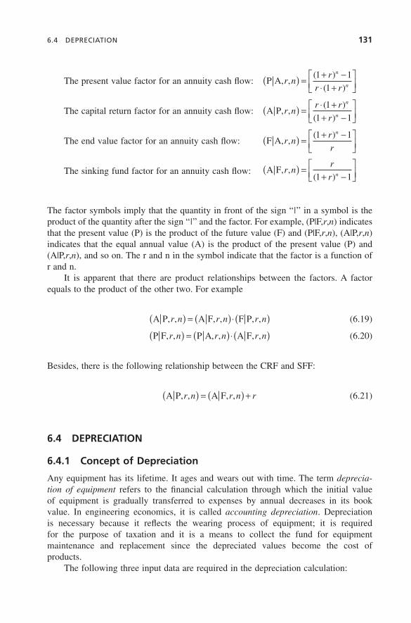
6.4 DEPRECIATION 131

The factor symbols imply that the quantity in front of the sign “ | ” in a symbol is the product of the quantity after the sign “ | ” and the factor. For example, (P | F, r , n ) indicates that the present value (P) is the product of the future value (F) and (P | F, r , n ), (A | P, r , n ) indicates that the equal annual value (A) is the product of the present value (P) and (A | P, r , n ), and so on. The r and n in the symbol indicate that the factor is a function of r and n.

It is apparent that there are product relationships between the factors. A factor equals to the product of the other two. For example

A P A F F P, , , , , ,r n r n r n( ) = ( )⋅ ( ) (6.19)

P F P A A F, , , , , ,r n r n r n( ) = ( )⋅ ( ) (6.20)

Besides, there is the following relationship between the CRF and SFF:

A P A F, , , ,r n r n r( ) = ( ) + (6.21)

6.4 DEPRECIATION

6.4.1 Concept of Depreciation

Any equipment has its lifetime. It ages and wears out with time. The term deprecia-tion of equipment refers to the fi nancial calculation through which the initial value of equipment is gradually transferred to expenses by annual decreases in its book value. In engineering economics, it is called accounting depreciation . Depreciation is necessary because it refl ects the wearing process of equipment; it is required for the purpose of taxation and it is a means to collect the fund for equipment maintenance and replacement since the depreciated values become the cost of products.

The following three input data are required in the depreciation calculation:

The present value factor for an annuity cash fl ow: P A, ,( )

( )r n

r

r r

n

n( ) = + −

⋅ +⎡⎣⎢

⎤⎦⎥

1 1

1

The capital return factor for an annuity cash fl ow: A P, ,( )

( )r n

r r

r

n

n( ) = ⋅ +

+ −⎡⎣⎢

⎤⎦⎥

1

1 1

The end value factor for an annuity cash fl ow: F A, ,( )

r nr

r

n

( ) = + −⎡⎣⎢

⎤⎦⎥

1 1

The sinking fund factor for an annuity cash fl ow: A F, ,( )

r nr

r n( ) =

+ −⎡⎣⎢

⎤⎦⎥1 1

c06.indd 131c06.indd 131 1/20/2011 10:26:03 AM1/20/2011 10:26:03 AM


• Basic cost of an asset

• Salvage value

• Depreciable life

The basic cost of an asset is the total cost incurred over its lifecycle, including the initial investment cost of the asset and maintenance cost over its life. The salvage value is an estimated value at the time of disposal. It is the value recovered through sale or reuse. If an asset does not have any value at disposal, the salvage value can be specifi ed to be zero. It is not easy to accurately estimate the salvage value. Besides, adjustments can be made in the process of depreciation if necessary.

There are the following four concepts of equipment life [84,85] :

• Physical Lifetime. A piece of equipment starts to operate from its brand new condition to a status in which it can no longer be used in the normal operating state and has to be retired. Maintenance activities can prolong its physical lifetime.

• Technical Lifetime. A piece of equipment may have to be replaced because of a technical progress, although it may still be used physically. For example, a new technology is developed for a type of equipment, and manufacturers no longer produce spare parts. This may result in such a situation that utilities cannot obtain necessary parts or the parts become too expensive for maintenance. Mechanical protection relays and mercury arc converters in HVDC systems are examples of the technical lifetime.

• Depreciable Lifetime. This refers to the timespan specifi ed for depreciation. By the end of the depreciable life, the fi nancial book value of equipment is depreci-ated to be a small salvage value. The depreciable life is sometimes called the useful life . A government specifi es the depreciable life in terms of different cat-egories of properties for the purpose of taxation. Utilities specify the depreciable life of various equipments on the basis of their fi nancial model.

• Economic Lifetime. By the end of the economic life, using a piece of equipment is no longer economical, although it may be still used physically and technically. This concept will be discussed further in Section 6.6 .

Several depreciation methods are discussed in the following subsections. It should be pointed out that maintenance and repairs can have effects on the basic cost and depre-ciable life. For instance, a maintenance activity may increase the basic cost of equip-ment and extend its depreciable life. In this case, an appropriate adjustment may be needed at some point of time in the depreciation calculation.

6.4.2 Straight - Line Method

The straight - line method [84] depreciates the value of an asset using an equal fraction of the basic cost in each year during the depreciation, which can be expressed as follows:

c06.indd 132c06.indd 132 1/20/2011 10:26:03 AM1/20/2011 10:26:03 AM


DI S

mk mk =

−=( , , )1… (6.22)

where D k is the depreciated value for year k ; I and S are the basic investment cost and salvage value, respectively; and m is the depreciable life (in years).

Obviously, the depreciated value is the same for each year during the depreciable life. The depreciation rate is defi ned by

α = 1

m (6.23)

In some literature, the depreciation rate in the straight - line method is defi ned as D k / I , which may not be accurate since the total value to be depreciated is I − S but not I .

The book value at the end of the k th year is

B I D k mk j

j

k

= − ==

∑1

1( , , )… (6.24)

6.4.3 Accelerating Methods

In accelerating methods [84] , the book value of equipment is depreciated more in early years than in later years. The accelerating methods are often used for the taxation purposes.

6.4.3.1 Declining Balance Method. In this method, the depreciated value in year k is calculated by

D I k mkk= ⋅ − =−α α( ) ( , , )1 11 … (6.25)

where α is the depreciation rate, I is the basic investment cost, and m is the depreciable life. Note that the concept of the depreciation rate in Equation (6.25) is different from that in the straight - line method.

The total depreciation (TD) up to year k can be calculated by

TDkj

j

k

k

I

I

= ⋅ −

= ⋅ − −

−

=∑α α

α

( )

[ ( ) ]

1

1 1

1

1

(6.26)

The book value at the end of the k th year is

B I I k mk kk= − = − =TD ( ) ( , , )1 1α … (6.27)

c06.indd 133c06.indd 133 1/20/2011 10:26:03 AM1/20/2011 10:26:03 AM


There are two approaches to determining the depreciation rate:

1. At the end of depreciable life (year m ), the book value should be equal to the salvage value. From Equation (6.27) , substituting the salvage value S for B k and m for k yields

S I m= −( )1 α (6.28)

The depreciation rate can be calculated by

α = − ⎛⎝⎜

⎞⎠⎟1

1S

I

m/

(6.29)

The defi ciency of this approach is that it cannot handle the situation in which the salvage value is zero.

2. The depreciation rate is prespecifi ed. For example, it can be specifi ed as

α β= ⋅ 1

m (6.30)

where β is a given factor, such as 1.5 or 2.0. This second approach can handle any situation in which the salvage value is or is not zero. In using the approach, however, the book value at the end of depreciable life (year m ) may be larger or smaller than the salvage value. If B m > S , an adjustment is conducted by switching to the straight - line method starting from the year in which the depreci-ated value obtained using the straight - line method is just larger than that obtained using the second approach. If B m < S , the book value is readjusted by stopping the depreciation in some year. This means that if the book value is lower than S in year k , the depreciated value in the k th year is adjusted so that B k = S and there is no more depreciation after year k .

6.4.3.2 Total Year Number Method. The total year number (TYN) is defi ned as follows:

TYN = = +

=∑ j

m m

j

m

1

1

2

( ) (6.31)

where m is the depreciable life. The depreciated value in year k is calculated by

Dm k

I S k mk =− +

− =1

1TYN

( ) ( , , )… (6.32)

c06.indd 134c06.indd 134 1/20/2011 10:26:03 AM1/20/2011 10:26:03 AM


The depreciation rate in year k is

αkm k= − +1

TYN (6.33)

Apparently, the depreciation rate is decreased every year. It is the remaining depreciable life divided by the total year number defi ned in Equation (6.31) .

The book value in each year can be calculated using Equation (6.24) .

6.4.4 Annuity Method

In the annuity method, the depreciated value in each year is equal to the equivalent annual cost minus the interest of the book value at the end of the previous year. The time value of cost is considered in this method.

The equivalent annual value can be calculated by the present value times the capital return factor, as shown in Equation (6.16) . The salvage value is the value at the end of depreciable life (year m ) and should be converted to its present value using Equation (6.8) . Therefore the equivalent annual value is

A I Sr

r r

rm

m

m= −

+⎡⎣⎢

⎤⎦⎥

⋅ ⋅ ++ −

⎡⎣⎢

⎤⎦⎥

1

1

1

1 1( )

( )

( ) (6.34)

where I and S are the basic initial investment cost and salvage value, respectively. Note that r should be the risk - free discount rate. In other words, it should be the r rkf or r int described in Section 6.3.1 .

The depreciated value in each year k is calculated by

D A r I

D A r I D k mk j

j

k

1

1

1

2

= − ⋅

= − ⋅ −⎡

⎣⎢⎢

⎤

⎦⎥⎥

==

−

∑ ( , , )… (6.35)

This method results in a decelerating depreciation process. The equipment value is depreciated less in early years than in later years.

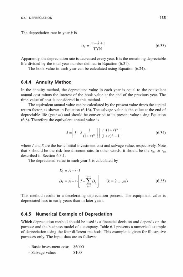
6.4.5 Numerical Example of Depreciation

Which depreciation method should be used is a fi nancial decision and depends on the purpose and the business model of a company. Table 6.1 presents a numerical example of depreciation using the four different methods. This example is given for illustrative purposes only. The input data are as follows:

• Basic investment cost: $6000 • Salvage value: $100

c06.indd 135c06.indd 135 1/20/2011 10:26:03 AM1/20/2011 10:26:03 AM


TABL

E 6.

1. D

epre

ciat

ed a

nd B

alan

ce V

alue

s (in

$) U

sing

the

Four

Dep

reci

atio

n M

etho

ds

Yea

r

Stra

ight

- Lin

e M

etho

d To

tal Y

ear

Num

ber

Met

hod

Dec

linin

g B

alan

ce M

etho

d A

nnui

ty M

etho

d

Dep

reci

ated

Val

ue

Bal

ance

D

epre

ciat

ed V

alue

B

alan

ce

Dep

reci

ated

Val

ue

Bal

ance

D

epre

ciat

ed V

alue

B

alan

ce

1 59

0.00

54

10.0

0 10

72.7

3 49

27.2

7 20

15.8

5 39

84.1

5 40

7.27

55

92.7

3 2

590.

00

4820

.00

965.

45

3961

.82

1338

.57

2645

.58

439.

86

5152

.87

3 59

0.00

42

30.0

0 85

8.18

31

03.6

4 88

8.85

17

56.7

3 47

5.04

46

77.8

3 4

590.

00

3640

.00

750.

91

2352

.73

590.

22

1166

.52

513.

05

4164

.78

5 59

0.00

30

50.0

0 64

3.64

17

09.0

9 39

1.92

77

4.60

55

4.09

36

10.6

9 6

590.

00

2460

.00

536.

36

1172

.73

260.

24

514.

35

598.

42

3012

.27

7 59

0.00

18

70.0

0 42

9.09

74

3.64

17

2.81

34

1.54

64

6.29

23

65.9

7 8

590.

00

1280

.00

321.

82

421.

82

114.

75

226.

79

698.

00

1667

.98

9 59

0.00

69

0.00

21

4.55

20

7.27

76

.20

150.

60

753.

84

914.

14

10

590.

00

100.

00

107.

27

100.

00

50.6

0 10

0.00

81

4.14

10

0.00

c06.indd 136c06.indd 136 1/20/2011 10:26:03 AM1/20/2011 10:26:03 AM

6.5 ECONOMIC ASSESSMENT OF INVESTMENT PROJECTS 137

It can be seen that all the four methods exactly reached the salvage value after 10 years ’ depreciation. The straight - line method provides the equal depreciated value in each year, the total year number and declining balance methods depreciate more in early years than in later years, and the annuity method depreciates less in early years than in later years.

6.5 ECONOMIC ASSESSMENT OF INVESTMENT PROJECTS

The purpose of conducting an economic assessment of investment projects is to provide an overall economic comparison between alternatives of a project or a ranking list for different projects. This information is the basis for decisionmakers to select the best alternative or project and justify or not justify an investment. There are three assessment methods:

• Total cost method

• Benefi t/cost analysis method

• Internal rate of return method

The basic concept of economic assessment has been briefl y summarized in Section 2.3.2 . This section provides more details. Note that all the methods focus on the relative economic comparison. If a project has a target for the improvement in system reliability or operation effi ciency, the target should be used as an additional condition in selecting a project or an alternative of a project.

6.5.1 Total Cost Method

The cash fl ows of three cost components (investment, operation, and unreliability costs) for each alternative are created. The present value of total cost (PVTC) is calcu-lated by

PVTC P F= + + ⋅( )=

∑ ( ) , ,I O R r kk k k

k

n

0

(6.36)

where I k , O k , and R k are the annual investment, operation, and unreliability costs in year k , respectively; r is the discount rate; and n is the length of cash fl ows (the number of years considered). Note that (P | F, r , k ) denotes the present value factor for a single future value. Its defi nition and the defi nition of (A | P, r , n ) used in Equation (6.37) have been given in Section 6.3.4.5 . Also, note that the costs at the year zero are included in Equation (6.36) .

• Depreciable life: 10 years • Interest rate: 0.08

c06.indd 137c06.indd 137 1/20/2011 10:26:03 AM1/20/2011 10:26:03 AM


Once the present value is obtained, it can be converted to the equivalent annual value (EAV) by

EAV PVTC A P= ⋅( ), ,r n (6.37)

The alternatives can be compared using either PVTC or EAV. It is important to appreci-ate the following three points:

1. In Equation (6.36) , I k is the annual investment cost required by a reinforcement alternative. There are two approaches for the annual operation cost O k and the annual unreliability cost R k . In the fi rst one, O k and R k are systemwide costs, meaning that these are the cost estimates for the whole system after an alterna-tive of a project is implemented. In the second one, O k (or R k ) is the incre-mental cost caused by a reinforcement alternative, that is, the difference between the system operation (or unreliability) costs with and without the alternative. The fi rst approach requires less calculation effort. Although the total cost obtained using the fi rst approach does not provide any clue about the cost of a project alternative, the total cost is meaningful for comparison purposes as the original system cost without any alternative is automatically canceled out in the comparison. The second approach requires more calcula-tions. This is because the operation or unreliability cost of a reinforcement alternative (such as addition of a line or transformer) is embedded in the system cost. The system analysis for calculating the incremental operation or unreliability cost due to a reinforcement alternative must be performed twice, once with the alternative and then without the alternative. The total cost obtained using the second approach provides information on pure cost of an alternative.

2. The investment cost of an alternative is always positive, whereas the operation or unreliability cost caused by an alternative may be either positive or negative. The operation cost includes different subcomponents as described in Section 6.1 , and some subcomponents may carry a negative cost. For example, an alternative may reduce network losses, which can be translated into a benefi t or a negative cost. If this benefi t is larger than other operation costs, the net operation cost becomes a negative value. In general, a transmission reinforce-ment alternative improves system reliability, but a system unreliability index cannot be reduced to be zero. Therefore, even if the system unreliability cost is reduced by an alternative, it is still positive when the fi rst approach is used. However, the incremental unreliability cost is normally negative when the second approach is used since the incremental reliability improvement due to an alternative is a benefi t. In some cases, a nonreinforcement alternative in transmission planning may lead to deterioration of system reliability. For example, when an independent power producer (IPP) is connected to the system, it may either improve or deteriorate system reliability depending on its location and connection manner.

c06.indd 138c06.indd 138 1/20/2011 10:26:03 AM1/20/2011 10:26:03 AM


3. The total cost method can be applied only to the ranking or comparison among alternatives of a project for resolving the same system problem. It cannot be applied to rank or compare projects for resolving different system problems.

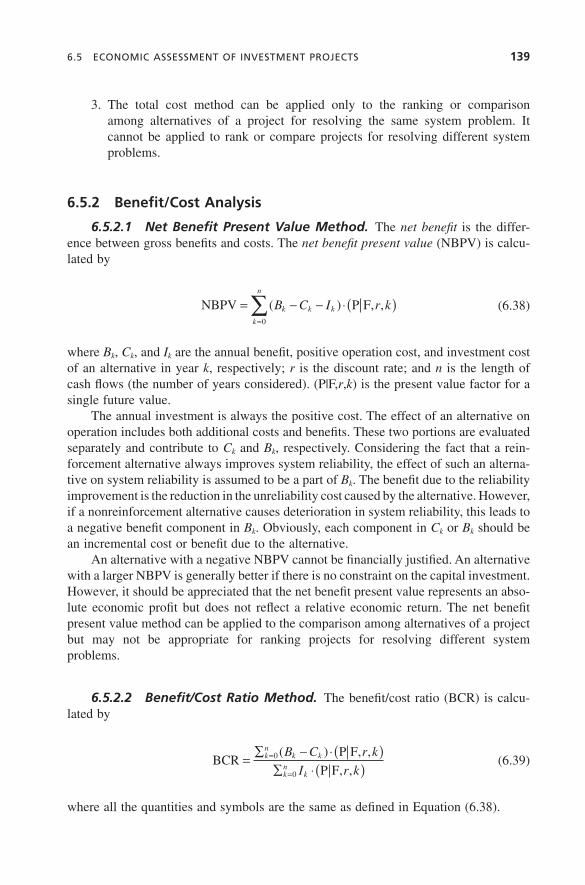
6.5.2 Benefi t/Cost Analysis

6.5.2.1 Net Benefi t Present Value Method. The net benefi t is the differ-ence between gross benefi ts and costs. The net benefi t present value (NBPV) is calcu-lated by

NBPV P F= − − ⋅( )=

∑ ( ) , ,B C I r kk k k

k

n

0

(6.38)

where B k , C k , and I k are the annual benefi t, positive operation cost, and investment cost of an alternative in year k , respectively; r is the discount rate; and n is the length of cash fl ows (the number of years considered). (P | F, r , k ) is the present value factor for a single future value.

The annual investment is always the positive cost. The effect of an alternative on operation includes both additional costs and benefi ts. These two portions are evaluated separately and contribute to C k and B k , respectively. Considering the fact that a rein-forcement alternative always improves system reliability, the effect of such an alterna-tive on system reliability is assumed to be a part of B k . The benefi t due to the reliability improvement is the reduction in the unreliability cost caused by the alternative. However, if a nonreinforcement alternative causes deterioration in system reliability, this leads to a negative benefi t component in B k . Obviously, each component in C k or B k should be an incremental cost or benefi t due to the alternative.

An alternative with a negative NBPV cannot be fi nancially justifi ed. An alternative with a larger NBPV is generally better if there is no constraint on the capital investment. However, it should be appreciated that the net benefi t present value represents an abso-lute economic profi t but does not refl ect a relative economic return. The net benefi t present value method can be applied to the comparison among alternatives of a project but may not be appropriate for ranking projects for resolving different system problems.

6.5.2.2 Benefi t/Cost Ratio Method. The benefi t/cost ratio (BCR) is calcu-lated by

BCRP F

P F= ∑ − ⋅( )

∑ ⋅( )=

=

kn

k k

kn

k

B C r k

I r k0

0

( ) , ,

, , (6.39)

where all the quantities and symbols are the same as defi ned in Equation (6.38) .

c06.indd 139c06.indd 139 1/20/2011 10:26:03 AM1/20/2011 10:26:03 AM


The benefi t cost ratio (BCR) represents the relative economic return, and the BCR method can be applied to the comparison among alternatives of a project or ranking among projects for resolving different system problems. The larger the BCR is, the better the project or alternative is. An alternative or project with a BCR < 1.0 cannot be fi nancially justifi ed. Utilities usually set a threshold value of BCR higher than 1.0 for justifi cation of projects or alternatives. For example, BCR > 1.5 or 2 is a frequently used threshold.

6.5.3 Internal Rate of Return Method

In general, an investment project has a positive net benefi t present value (NBPV). It can be proved from Equation (6.38) that the NBPV decreases as the discount rate increases. This indicates that if a larger discount rate is used, it will be more diffi cult to justify a project or alternative. Selecting an appropriate discount rate is an important fi nancial decision for utilities. Utilities select the value of discount rate on the basis of multiple factors, including their business model.

The internal rate of return (IRR) is defi ned as the break - even discount rate leading to NBPV = 0. In other words, the IRR is the solution r * of the following equation

NBPV P F *= − − ⋅( ) ==

∑ ( ) , ,B C I r kk k k

k

n

0

0 (6.40)

where all the quantities and symbols are the same as defi ned in Equation (6.38) , except that r * is the unknown IRR.

A bisection algorithm can be used to fi nd IRR. Two initial r values are selected such that one leads to a positive NBPV and another to a negative NBPV. The average of these two r values is used to calculate a new NBPV. The original r that causes NBPV to have a sign opposite that of the new NBPV is kept and the other is relinquished. The new r and the retained original r are used in the next iteration until a solution is found.

Mathematically, Equation (6.40) can have multiple solutions if the annual amounts in a net benefi t cash fl ow change their signs (from positive to negative or vice versa) more than once. This is a demerit of the IRR method. However, the majority of actual projects have a net benefi t cash fl ow in which the annual amounts do not change the sign or change it only once, resulting in a unique real number solution of IRR.

If the IRR for a project or alternative is smaller than the minimum discount rate that has been selected by a utility for its fi nancial analysis, the project or alternative is not fi nancially justifi able since this implies that the utility ’ s discount rate will result in a negative NBPV.

When two projects or alternatives are compared, the concept of incremental inter-nal rate of return (IIRR) is introduced. The IIRR is defi ned as the discount rate that makes the net benefi t present values of the two projects or alternatives equal, that is

( ) , , ( ) , ,B C I r k B C I r kk k k

k

n

k k k

k

n

1 1 1

0

2 2 2

0

− − ⋅ ′( ) − − − ⋅ ′( ) == =

∑ ∑P F P F 00 (6.41)

c06.indd 140c06.indd 140 1/20/2011 10:26:03 AM1/20/2011 10:26:03 AM


where all the quantities and symbols are similar to those defi ned in Equation (6.38) , the subscript 1 or 2 represents the fi rst or second project or alternative, and ′r is the IIRR that satisfi es Equation (6.41) .

Equation (6.41) can be rewritten as follows:

( ) , , ( ) ( ) , ,B B r k C I C I r kk k

k

n

k k k k

k

n

1 2

0

1 1 2 2

0

− ⋅ ′( ) = + − + ⋅ ′( )= =

∑ P F P F∑∑ (6.41a)

Equation (6.41a) indicates that the present value of incremental benefi t between the two projects or alternatives is equal to the present value of incremental cost between the two at the IIRR.

If a project or alternative requires a lower cost but creates a higher return (benefi t) than the other does, this project or alternative is certainly better. However, a confl ict situation may occur: a project or alternative may require a higher cost with a higher return. In this case, the IIRR can be used as a criterion as follows. If ′r is larger than the minimum discount rate selected by the utility for its fi nancial analysis, the project or alternative with a higher investment and a higher return is better. Otherwise, if ′r is smaller than the utility ’ s discount rate, the project or alternative with a lower investment and a lower return is better.

When multiple projects or alternatives are compared, the following procedure is used:

1. The internal rates of return for all alternatives or projects are calculated. The alternatives or projects with the IRR smaller than the utility ’ s discount rate are not justifi able and are excluded from further consideration.

2. The remaining alternatives or projects are listed in order of increasing invest-ment cost.

3. The fi rst two alternatives or projects are compared using their IIRR, and the better one is determined.

4. The alternative or project with the better IIRR selected in step 3 is compared with the third alternative or project. The process proceeds until all alternatives or projects have been compared.

6.5.4 Length of Cash Flows

The length of cash fl ows needs to be predetermined in using any of the methods dis-cussed above. It is a challenge issue to determine the number of years to be considered [i.e., n in Equations (6.36) – (6.41) ]. In engineering economics, it has been suggested that n should be the useful (depreciable) life of a project or alternative. Unfortunately, there are diffi culties in using the useful life as the length of cash fl ows for transmission planning projects. This is not just because different alternatives or projects may have different useful lives. A more crucial reason is because the useful life of transmission equipment in a project or alternative is generally very long, such as 40 – 50 years for a transformer and much longer for an overhead line. It is impossible to evaluate operation

c06.indd 141c06.indd 141 1/20/2011 10:26:04 AM1/20/2011 10:26:04 AM


and unreliability costs of the system over such a long time period since there is no system information (load forecast and other system conditions) available beyond the planning period, which may range from only several to 20 years. Usually, other future projects will be added to the system after a project is implemented but the future proj-ects are unknown at the current time when a project is planned. This results in diffi culty or inability to evaluate the effect of a project or alternative on operation and unreliability costs beyond the planning period.

It is suggested that the planning period be used for the length (the number of years) of cash fl ows for transmission projects. However, the effect of initial total investment cost spreads over the useful life and does not stop at the end of the planning period. When the initial total investment cost is converted into equivalent annual investment costs on a cash fl ow using the capital return factor, the timespan of this cash fl ow is still its useful life. Two approaches can be used to deal with this inconsistency. In the fi rst one, the equivalent annual investment costs beyond the planning period are con-sidered by introducing an equivalent salvage value at the end of the planning period. The demerit of doing so is the fact that the effects of a project or alternative on system operation and reliability beyond the planning period are ignored, but the effect of its investment beyond the planning period is still included. This implies that the possible positive effects of a project or alternative on system operation and reliability is under-estimated. In the second approach, the effect of investment cost beyond the planning period is also ignored. This approach is normally acceptable in actual applications, particularly for a long planning period since the effect of a salvage value is small. In general, the second approach is better, although an adjustment may be needed for a short planning period in some cases.

6.6 ECONOMIC ASSESSMENT OF EQUIPMENT REPLACEMENT

The majority of system planning projects are associated with equipment addition. However, an economic analysis is also performed on the projects for replacement of existing equipment. Two frequent issues in replacement planning are (1) whether an old or aged facility should be replaced and (2) if so, when it should be replaced. The purpose of economic assessment for equipment replacement is to address these two issues.

6.6.1 Replacement Delay Analysis

The current year is used as a reference point. If a replacement is performed in the current year, the net investment cost is the capital cost of new equipment minus the salvage value of old equipment. If the replacement is delayed by n * year, there are two impacts. On one hand, the operation and unreliability costs incurred by continuously using the old equipment are higher than those incurred by using the new equipment. We have to pay the increased operation and unreliability costs. On the other hand, we save the interests of the investment cost of new equipment for n * years. Note that the capital investment is still required n * later and we cannot save the whole investment

c06.indd 142c06.indd 142 1/20/2011 10:26:04 AM1/20/2011 10:26:04 AM

6.6 ECONOMIC ASSESSMENT OF EQUIPMENT REPLACEMENT 143

by delaying the replacement. The salvage value of old equipment will be decreased and the difference in the salvage value between the current year and year n * should be taken away from the saved interests. If the increased costs are higher than the saved interests, the replacement should not be delayed further. This idea can be mathematically expressed by

( ) ( ) ( ) ( )*

*

*

OE OR RE RR i I i S Sk k k k

k

nk

n

k

n

− + − > ⋅ ⋅ + − −=

−

=∑ ∑

1

10

1

1 (6.42)

where OE k and OR k are the operation costs required by existing (old) and replacement (new) equipment in year k , respectively; RE k and RR k are the unreliability costs incurred by using existing and replacement equipments in year k , respectively; I is the initial total investment cost of replacement equipment; S 0 and S n * are the salvage values of existing equipment in the current year and year n * , respectively; i is the risk - free annual real interest rate (i.e., r int discussed in Section 6.3.1 ); and n * is the number of years to be determined for replacement delay. The saved interests are calculated by considering a compound rate approach.

The annual operation cost includes the subcomponents that are different in value for existing and replacement equipment (such as maintenance and repair costs), whereas the subcomponents that have the same value for existing and replacement equipment (such as network losses) can be excluded from the annual operation cost. The annual unreliability cost refers to the incremental damage cost due to random failures of exist-ing or replacement equipment. Obviously, the existing equipment will cause a higher unreliability cost than will the new equipment because an old facility generally has greater unavailability. A replacement occurs at the stage near the end of life of existing equipment, and the salvage value is always small. In most cases, the term ( S 0 − S n * ) is negligible.

The minimum n * that satisfi es inequality (6.42) is the number of years for which the replacement should be delayed. The procedure to fi nd the minimum n * is simple. Let n * = 1 fi rst. If the inequality in Equation (6.42) is not satisfi ed, let n * = 2 and recheck it, and so on. The process proceeds until the inequality in Equation (6.42) is just satisfi ed.

6.6.2 Estimating Economic Life

The equivalent annual investment cost (EAIC) over m * years, which is often called the annual capital recovery cost , can be calculated by

EAIC A P * A F *= ⋅( ) − ⋅( )I r m S r mm, , , ,* (6.43)

where I is the initial total investment, S m * is the salvage value at the end of m * years, r is the discount rate, and m * is the economic life (in years) that needs to be found.

The equivalent annual operation and unreliability cost (EAOUC) incurred by a piece of equipment over m * years can be calculated by

c06.indd 143c06.indd 143 1/20/2011 10:26:04 AM1/20/2011 10:26:04 AM


EAOUC P F A P= + ⋅( )⎛⎝⎜

⎞⎠⎟

⋅ ( )=

∑ ( ) , , , , **

O R r k r mk k

k

m

0

(6.44)

where O k and R k are the annual operation and unreliability costs incurred by the equip-ment in year k . Note that the R k should be an incremental cost, which is the difference in the system unreliability cost between the two cases with considering and not con-sidering the failure of the equipment. If the network loss due to the equipment is a part of O k , this part should also be an incremental network loss cost due only to the equip-ment, which could be either positive or negative.

The total equivalent annual cost (TEAC) is the sum of EAIC and EAOUC. The salvage value is always a small amount at the end of economic life and is often negligible compared to the investment cost. The EAIC is a decreasing function of the parameter m * . In other words, the longer a piece of equipment is used, the smaller the EAIC becomes. On the other hand, the EAOUC is an increasing function of the parameter m * . This is because both the operation and unreliability costs increase as equipment ages because of increased OMA costs and unavailability of equipment in an aging status. Therefore, the TEAC is a convex function of m * with a unique minimum point. According to the defi nition given in Section 6.4.1 , the economic life is the length of time in years by the end of which the total equivalent annual cost (TEAC) reaches the minimum point. In other words, the economic life is the m * that minimizes the TEAC.

The procedure to fi nd the economic life m * is straightforward. The TEAC is cal-culated by letting m * = 1,2,3, … , and so on. The minimum TEAC can be observed in the series of TEAC values. The year corresponding to the minimum TEAC is the eco-nomic life.

Conceptually, the economic life can be regarded the year in which a replacement should take place. However, this criterion alone should be used with caution if the economic life has been calculated at an early stage of equipment in service. The esti-mated operation and unreliability costs for many future years will be very inaccurate. The discount rate is also uncertain and may vary over the life. Nevertheless, the esti-mated economic life is useful information even if it is not accurate. It can be reestimated as time advances. The economic life can be combined with the replacement delay analysis in actual applications. The economic life of equipment is estimated fi rst, and then the replacement delay analysis method is applied when the service year of equip-ment approaches the end of the economic life.

6.7 UNCERTAINTY ANALYSIS IN ECONOMIC ASSESSMENT

There are uncertainties for the input data in the economic analysis, including the dis-count rate, useful life, salvage value, and estimates of investment, operation, and unreli-ability costs. The uncertainties of the input data create the uncertainties of the outputs, including the depreciated and book values, present and annual values, and outputs used for comparisons between alternatives or projects. Two methods can be used to deal with the uncertainties: sensitivity analysis and probabilistic techniques.

c06.indd 144c06.indd 144 1/20/2011 10:26:04 AM1/20/2011 10:26:04 AM

6.7 UNCERTAINTY ANALYSIS IN ECONOMIC ASSESSMENT 145

6.7.1 Sensitivity Analysis

Sensitivity analysis is straightforward. This is based on the concept of incremental change — if a variation of an input data is given, what would be the variation in an output?

For example, if we want to obtain the sensitivity of the present value of total cost (PVTC) to the discount rate in Equation (6.36) , we can specify different variations of discount rate and calculate a series of values of PVTC. The same idea can apply to the sensitivity between any input and any output.

The advantage of sensitivity analysis is simplicity. However, it has two demerits: (1) it provides the sensitivity of an output to only one input variable at a time — any change in output caused by simultaneous variations of two or more input variables will create unclear information; and (2) it cannot provide a single mean value of output considering uncertainties of all input data.

6.7.2 Probabilistic Analysis

The probabilistic analysis method in the economic assessment includes the following steps:

• A discrete probability distribution representing the uncertainty of an input data is obtained either by the estimation from engineering judgment (subjective prob-ability) or by statistical records (objective probability).

• Multiple values of an output are calculated for all possible values of input data defi ned in the discrete probability distribution using the relevant formulas or calculation processes in the economic assessment.

• The mean value and standard deviation of the output are calculated.

• A fi nancial risk assessment for planning projects or alternatives is performed.

The net benefi t present value (NBPV) in Equation (6.38) is used as an example. It is assumed that the discount rate r has the following discrete probability distribution

p r r p i Ni i r( ) ( , , )= = = 1… (6.45)

where r is a random variable of discount rate. The discrete probability distribution indicates that r has N r possible values and each one has a probability of p i . This probabil-ity distribution can be estimated from the historical records of interest and infl ation rates that were used in the fi nancial analysis of a utility.

The N r values of NBPV for a planning alternative are calculated using Equation (6.38) from N r values of r . The mean and standard deviation of NBPV for the alterna-tive is calculated by

E r pi i

i

N

i

r

( ) ( )NBPV NBPV= ⋅=

∑1

(6.46)

c06.indd 145c06.indd 145 1/20/2011 10:26:04 AM1/20/2011 10:26:04 AM


Std NBPV NBPV NBPV( ) [ ( )]= − ⋅=

∑ i

i

N

iE pr

2

1

(6.47)

Let us look at how to consider the uncertainties of both useful life and discount rate for a planning alternative. The equivalent annual investment cost for the alternative can be calculated using the initial total investment cost and the capital return factor by

I Ir r

rk

m

m= ⋅ ⋅ +

+ −⎡⎣⎢

⎤⎦⎥

( )

( )

1

1 1 (6.48)

where I and I k are the initial total investment and equivalent annual investment costs, respectively; r is the discount rate; and m is the useful life of the alternative.

It is assumed that the useful life has N s possible estimates m j ( j = 1, … , N s ) and each estimated value has an equal possibility (i.e., the subjective probability for each value is 1/ N s ). With N r values of r and N s values of m , the N r × N s values of I k can be obtained from Equation (6.48) fi rst and then the N r × N s values of NBPV for the alternative are calculated using Equation (6.38) . The mean and standard deviation of NBPV for the alternative is calculated by

EN

r m ps

ij i j

j

N

i

N

i

sr

( ) ( , )NBPV NBPV= ⋅==

∑∑1

11

(6.49)

where NBPV ij is the value of NBPV for r i and m j . Its standard deviation is estimated by

Std NBPV NBPV NBPV( ) [ ( )]= − ⋅==

∑∑1 2

11N

E ps

ij

j

N

i

N

i

sr

(6.50)

The method described above can be easily extended to a case where the uncertainties of more than two input data need to be considered.

In comparing different alternatives, the same discrete probability distribution of discount rate should be used. However, the discrete probability distributions of other input data (such as the useful life) can be different. With the results from the probabi-listic analysis, both the mean value and standard deviation of NBPV should be consid-ered in the comparison between alternatives. Obviously, if two alternatives have very close standard deviations of NBPV, the one with a larger mean value of NBPV is better as it creates more net benefi ts. If two alternatives have the very close mean values of NBPV, the one with a smaller standard deviation is better because it carries a lower fi nancial risk. It is possible that one alternative has a larger mean value of NBPV with a larger standard deviation but another has a smaller mean value of NBPV with a smaller standard deviation. In this case, an engineering judgment is needed. This is associated with a compromise between benefi t and fi nancial risk.

The procedure for the probabilistic analysis method for other economic assess-ments is similar to that for the NBPV described above.

c06.indd 146c06.indd 146 1/20/2011 10:26:04 AM1/20/2011 10:26:04 AM

6.8 CONCLUSIONS 147

6.8 CONCLUSIONS

This chapter discussed the economic analysis methods in transmission planning. The investment and operation costs are the basic components in general engineering eco-nomics, whereas the unreliability cost is a special component that needs to be added in the economic assessment for transmission system planning. The incorporation of this component requires modifi ed concepts in the economic analysis. It is important to appre-ciate that the unreliability cost and some subcomponents of operation cost due to an alternative or a piece of equipment should be calculated using an incremental approach.

The time value of money, which originates from the interest and infl ation, is the basis of engineering economics. The discount rate in discounting calculations can be a nominal or real interest rate depending on whether an infl ation rate is included. It can be either a risk - free rate or risky rate depending on whether the fi nancial risk is con-sidered in a project. The six factors for conversion between the present, annual, and future values are all based on the time value of money. Depreciation is another impor-tant concept in the economic analysis. The investment cost, depreciable (useful) life, and salvage value are the three input data needed to calculate the annual depreciated and book values of equipment. Different depreciation methods provide varied (equal, accelerating, or decelerating) annual depreciation rates. Which method should be used depends on fi nancial considerations and business models of utilities.

The economic assessment of investment projects is at the core of economic analysis in transmission planning. The purpose is to provide the decisionmaking information in determining the fi nal alternative of a planning project or ranking different projects. The total cost method and the net benefi t present value method can be used for the com-parison between alternatives of a project but are not appropriate for ranking projects intended to resolve different system problems because they provide the information only on absolute economic profi t. The benefi t/cost ratio method and the internal rate of return method can be used in the justifi cation of a project or alternative, comparison between alternatives of a project, and ranking among different projects as they provide the information of relative economic return.

The best time of replacement can be decided using the economic assessment of equipment replacement. The replacement delay analysis method is used when a piece of equipment approaches the end - of - life stage at which more accurate data become available. Although the economic life of equipment can be estimated even at an early stage of equipment service, it is not accurate because of inaccuracy of data for future years. The combined use of the economic life estimation and the replacement delay analysis method provides a better result.

There are always uncertainties of input data in the economic assessment. Sensitivity and probabilistic analysis methods can be used to deal with the uncertainties. The probabilistic techniques create the mean value and standard deviation of economic indices for a planning project or alternative. Both the mean and standard deviation provide essential information in decisionmaking. The mean value is used to judge the economic profi t of a project or alternative, whereas the standard deviation is an indicator of its fi nancial risk level.

c06.indd 147c06.indd 147 1/20/2011 10:26:04 AM1/20/2011 10:26:04 AM

Documents

Probabilistic Transmission System Planning (Li/Transmission System Planning) || Economic Analysis Methods