Probabilistic Transmission System Planning (Li/Transmission System Planning) || Appendix C: Elements of Reliability Evaluation

329

C.1 BASIC CONCEPTS

C.1.1 Reliability Functions

Reliability can be represented using a probability distribution as

R t f t dtt

( ) ( )=∞

∫ (C.1)

where f ( t ) is the failure probability density function. The inverse operation of (C.1) gives

f tdR t

dt( )

( )= − (C.2)

Unreliability can be expressed as

Q t R t f t dtt

( ) ( ) ( )= − = ∫10

(C.3)

APPENDIX C

ELEMENTS OF RELIABILITY EVALUATION

Probabilistic Transmission System Planning, by Wenyuan LiCopyright © 2011 Institute of Electrical and Electronics Engineers

bapp03.indd 329bapp03.indd 329 1/20/2011 10:23:41 AM1/20/2011 10:23:41 AM

330 ELEMENTS OF RELIABILITY EVALUATION

The mean time to failure can be calculated by

MTTF = =∞ ∞

∫ ∫tf t dt R t dt( ) ( )0 0

(C.4)

The failure rate is defi ned as

λ( )( )

( )t

f t

R t= (C.5)

By substituting Equation (C.2) into Equation (C.5) , we can also represent reliability using the failure rate function as

R t t dtt

( ) exp ( )= −⎡⎣⎢

⎤⎦⎥∫ λ

0 (C.6)

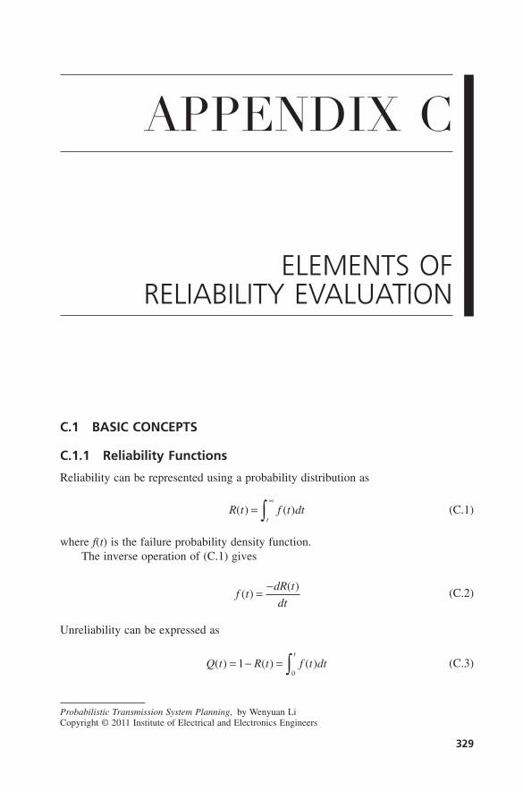
C.1.2 Model of Repairable Component

Components are classifi ed into nonrepairable and repairable categories. A power system component is repairable in the normal life period and can die at the end - of - life stage. For a repairable component, reliability and availability are two different concepts. Reliability is the probability that a component has not failed as of a given time point, whereas availability is the probability that a component is found available at a given time point although it may have experienced failures and repairs before this point. If the exponential distribution is used to model the failure and repair processes, a repair-able component has constant failure and repair rates. Figure C.1 shows the state transi-tion model of a repairable component.

The failure rate λ , repair rate μ , and failure frequency f are calculated by

λ = 1

d (C.7)

μ = 1

r (C.8)

fd r

=+1

(C.9)

where d and r are the mean time to failure and mean time to repair, respectively.

Figure C.1. Two - state model of a repairable component.

λ

µ

Up state Down state


C.2 CRISP RELIABILITY EVALUATION 331

The average unavailability is calculated by

U f r=+

= ⋅λλ μ

(C.10)

The failure rate and failure frequency have the following relationship:

fr

=+λλ1

(C.11)

In most engineering applications, f and λ are numerically close since λ and r are both small values.

Note that in the equations above, the unit of λ , μ , or f is in occurrences/year and the unit of d or r is in years.

C.2 CRISP RELIABILITY EVALUATION

C.2.1 Series and Parallel Networks

Components are said to be in series if only one needs to fail for the network failure, or they must be all up for the network success. Components are said to be in parallel if they must all fail for the network failure, or only one needs to be up for the network success.

In this section, U , λ , μ , f , and r are the same as defi ned in Section C.1.2 except that the subscript 1 or 2 represents component 1 or 2. A denotes availability, which equals 1 − U . The subscripts “ se ” and “ pa ” represent series and parallel networks, respectively.

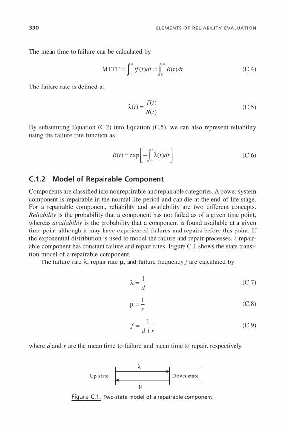
C.2.1.1 Series Network. Consider the case of two repairable components in series as shown in Figure C.2 .

From the defi nition of the series network, the following relationships hold:

U U U U Use = + −1 2 1 2 (C.12)

λ λ λse = +1 2 (C.13)

A A Ase = 1 2 (C.14)

The equivalent repair time and failure frequency for the series network can be derived and expressed as follows:

Figure C.2. Series network and its equivalence.

λ1, r1 λ2, r2 λse, rse



rr r r r

se =+ +

+λ λ λ λ

λ λ1 1 2 2 1 1 2 2

1 2

(C.15)

f f f r f f rse = − + −1 2 2 2 1 11 1( ) ( ) (C.16)

In most engineering applications, because failure rates ( λ ) and repair times ( r ) are small values, Equation (C.15) can be approximated by

rr r

se ≈++

λ λλ λ1 1 2 2

1 2

(C.17)

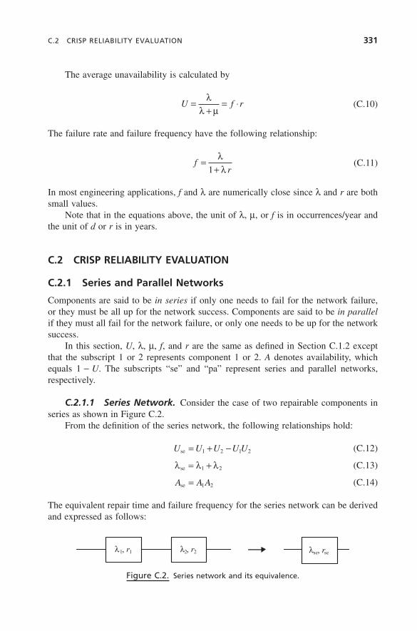
C.2.1.2 Parallel Network. Figure C.3 shows the case of two repairable com-ponents in parallel.

From the defi nition of the parallel network, the following relationships hold:

U U Upa = 1 2 (C.18)

μ μ μpa = +1 2 (C.19)

A A A A Apa = + −1 2 1 2 (C.20)

The equivalent repair time, failure rate, and failure frequency for the parallel network can be derived and expressed as:

rr r

r rpa =

+1 2

1 2

(C.21)

λλ λ

λ λpa =+

+ +1 2 1 2

1 1 2 21

( )r r

r r (C.22)

f f f r rpa = +1 2 1 2( ) (C.23)

In most engineering applications, because λ r << 1, Equation (C.22) can be approxi-mated by

λ λ λpa = +1 2 1 2( )r r (C.24)

Figure C.3. Parallel network and its equivalence.

λ1, r1

λ2, r2

λpa, rpa


C.2 CRISP RELIABILITY EVALUATION 333

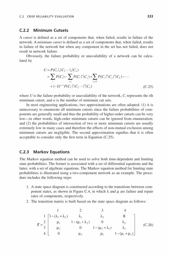
C.2.2 Minimum Cutsets

A cutset is defi ned as a set of components that, when failed, results in failure of the network. A minimum cutset is defi ned as a set of components that, when failed, results in failure of the network but when any component in the set has not failed, does not result in network failure.

Obviously, the failure probability or unavailability of a network can be calcu-lated by

U P C C C

P C P C C P C C C

n

i

i

i j

i j

i j k

i j k

=

= − + −

+ −

∑ ∑ ∑( )

( ) ( ) ( )

(

, , ,

1 2∪ �∪

∩ ∩ ∩ �

11 11 2) ( )n

nP C C C− ∩ �∩ (C.25)

where U is the failure probability or unavailability of the network, C i represents the i th minimum cutset, and n is the number of minimum cut sets.

In most engineering applications, two approximations are often adopted: (1) it is unnecessary to enumerate all minimum cutsets since the failure probabilities of com-ponents are generally small and thus the probability of higher - order cutsets can be very low — in other words, high - order minimum cutsets can be ignored from enumeration; and (2) the probabilities of intersection of two or more minimum cutsets are usually extremely low in many cases and therefore the effects of non - mutual exclusion among minimum cutsets are negligible. The second approximation signifi es that it is often acceptable to consider only the fi rst term in Equation (C.25) .

C.2.3 Markov Equations

The Markov equation method can be used to solve both time - dependent and limiting state probabilities. The former is associated with a set of differential equations and the latter, with a set of algebraic equations. The Markov equation method for limiting state probabilities is illustrated using a two - component network as an example. The proce-dure includes the following steps:

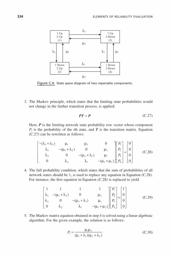
1. A state space diagram is constructed according to the transitions between com-ponent states, as shown in Figure C.4 , in which λ and μ are failure and repair rates of components, respectively.

2. The transition matrix is built based on the state space diagram as follows:

T =

− +⎡

⎣

⎢⎢⎢⎢

− +− +

1 2 3 4

1

2

3

4

1

0

1

0

0

1

1 2

1

2

1

1 2

2

2

2 1

1

( )

( )

( )

λ λμμ

λμ λ

μ

λ

μ λμ

00

1

2

1

1 2

λλ

μ μ− +

⎤

⎦

⎥⎥⎥⎥

( )

(C.26)



3. The Markov principle, which states that the limiting state probabilities would not change in the further transition process, is applied:

PT P= (C.27)

Here, P is the limiting network state probability row vector whose component P i is the probability of the i th state, and T is the transition matrix. Equation (C.27) can be rewritten as follows:

− +− +

− +− +

⎡

⎣

⎢⎢⎢⎢

( )

( )

( )

( )

λ λ μ μλ μ λ μλ μ λ μ

λ λ μ μ

1 2 1 2

1 1 2 2

2 2 1 1

2 1 1 2

0

0

0

0

⎤⎤

⎦

⎥⎥⎥⎥

⎡

⎣

⎢⎢⎢⎢

⎤

⎦

⎥⎥⎥⎥

=

⎡

⎣

⎢⎢⎢⎢

⎤

⎦

⎥⎥⎥⎥

P

P

P

P

1

2

3

4

0

0

0

0

(C.28)

4. The full probability condition, which states that the sum of probabilities of all network states should be 1, is used to replace any equation in Equation (C.28) . For instance, the fi rst equation in Equation (C.28) is replaced to yield

1 1 1 1

0

0

0

1 1 2 2

2 2 1 1

2 1 1 2

1

λ μ λ μλ μ λ μ

λ λ μ μ

− +− +

− +

⎡

⎣

⎢⎢⎢⎢

⎤

⎦

⎥⎥⎥⎥

( )

( )

( )

P

P22

3

4

1

0

0

0

P

P

⎡

⎣

⎢⎢⎢⎢

⎤

⎦

⎥⎥⎥⎥

=

⎡

⎣

⎢⎢⎢⎢

⎤

⎦

⎥⎥⎥⎥

(C.29)

5. The Markov matrix equation obtained in step 4 is solved using a linear algebraic algorithm. For the given example, the solution is as follows:

P11 2

1 1 2 2

=+ +

μ μμ λ μ λ( )( )

(C.30)

Figure C.4. State space diagram of two repairable components.

λ2

μ2

λ1 μ1 λ1 μ1

λ2

μ2

1 Up 2 Up (1)

1 Up 2 Down

(3)

1 Down 2 Up (2)

1 Down 2 Down

(4)


C.3 FUZZY RELIABILITY EVALUATION 335

P21 2

1 1 2 2

=+ +

λ μμ λ μ λ( )( )

(C.31)

P31 2

1 1 2 2

=+ +

μ λμ λ μ λ( )( )

(C.32)

P41 2

1 1 2 2

=+ +

λ λμ λ μ λ( )( )

(C.33)

Once the probability P i of the i th state is obtained by the Markov method, the frequency f i of encountering the state is calculated by

f Pi i k

k

Mi

==

∑λ1

(C.34)

where λ k is the departing transition (failure or repair) rate; M i is the number of the transition rates departing from the i th state.

The probability P , frequency f , and duration D of a state or state set satisfy the following generic relationship:

P f D= ⋅ (C.35)

The mean duration of residing a state or state set can be calculated from the state prob-ability and frequency.

C.3 FUZZY RELIABILITY EVALUATION

C.3.1 Series and Parallel Networks Using Fuzzy Numbers

In the nofuzzy reliability evaluation, the unreliability U pa of a parallel network with n components can have a general expression as follows [see Equation (C.18) ]:

U Ui

i

n

pa ==

∏1

(C.36)

Here, U i is the unreliability of the i th component, which represents the failure probabil-ity of each component when a nonrepairable network is evaluated, or the unavailability of each component when a repairable network is evaluated.

It is assumed that the unreliability of each component is modeled by a triangular fuzzy number: U i = ( a i 1 , a i 2 , a i 3 ). Its α cut is calculated by

( ) [ ( ), ( )]U a a a a a ai i i i i i iα α α= + − − −1 2 1 3 3 2 (C.37)

Using the rule given in Equation (B.14) , the α cut of the unreliability for a parallel network can be directly calculated by



( ) ( )

( ( )), ( ( ))

U U

a a a a a a

i

i

n

i i i

i

n

i i i

i

pa α α

α α

=

= + − − −

=

= =

∏

∏1

1 2 1

1

3 3 2

11

n

∏⎡

⎣⎢

⎤

⎦⎥ (C.38)

In the nonfuzzy reliability evaluation, the unreliability of a series network with n com-ponents can have a general expression as follows [see Equation (C.14) ]:

U A Ui

i

n

i

i

n

se = − = − −= =

∏ ∏1 1 11 1

( ) (C.39)

Using the rules given in Equations (B.12) and (B.14) , the α cut of the unreliability for a series network is calculated by

( ) , , ( )

, ( ),

U U

a a a a

i

i

n

i i i

se α α

α

= [ ]− [ ]−{ }

= [ ]− − + − −

=∏1 1 1 1

1 1 1 1

1

3 3 2 ii i i

i

n

i i i i i

a a

a a a a a a

1 2 1

1

1 2 1 3 31 1 1 1

− −[ ]

= − − − −{ } − − + −

=∏ α

α α

( )

( ) , ( ii

i

n

i

n

2

11

){ }⎡

⎣⎢

⎤

⎦⎥

==∏∏ (C.40)

It should be pointed out that in transmission system reliability evaluation, the input data are often given by outage frequencies and repair times of components. In this case, Equation (C.10) is used to calculate the unavailability of a component from the outage frequency and repair time. If the outage frequency and repair time are expressed using triangular fuzzy numbers, the arithmetic operation rules in Section B.2.2 can be applied to Equation (C.10) . Note that the membership function of unavailability is no longer triangular, even if both the outage frequency and repair time have triangular member-ship functions. This does not affect calculations as the arithmetic operation rules can be individually applied to each discrete membership function grade (i.e., α cut).

C.3.2 Minimum Cutset Approach Using Fuzzy Numbers

It is diffi cult to apply fuzzy calculations to the terms in Equation (C.25) , which are associated with nonmutual exclusion among minimum cutsets. As pointed out in Section C.2.2 , however, the effects of nonmutual exclusion are negligible in most engineering applications, including transmission reliability evaluation. Therefore, an approximate method can be considered.

A second - order or higher - order minimum cutset contains more than one compo-nent. Each minimum cutset is composed of components in parallel since all the com-ponents in the set must fail for the set failure. All minimum cutsets are in series as only one of them needs to fail for the network failure. As such, a combination of minimum



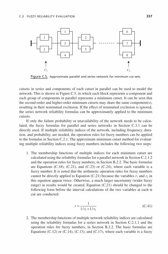
cutsets in series and components of each cutset in parallel can be used to model the network. This is shown in Figure C.5 , in which each block represents a component and each group of components in parallel represents a minimum cutset. It can be seen that the second - order and higher - order minimum cutsets may share the same component(s), resulting in their nonmutual exclusion. If the effect of nonmutual exclusion is ignored, the series network reliability formulas can be approximately applied to the minimum cutsets.

If only the failure probability or unavailability of the network needs to be calcu-lated, the fuzzy formulas for parallel and series networks in Section C.3.1 can be directly used. If multiple reliability indices of the network, including frequency, dura-tion, and probability, are needed, the operation rules for fuzzy numbers can be applied to the formulas in Section C.2.1 . The approximate minimum cutset method for evaluat-ing multiple reliability indices using fuzzy numbers includes the following two steps:

1. The membership functions of multiple indices for each minimum cutset are calculated using the reliability formulas for a parallel network in Section C.2.1.2 and the operation rules for fuzzy numbers, in Section B.2.2 . The basic formulas are Equations (C.18) , (C.21) , and (C.23) or (C.24) , where each variable is a fuzzy number. It is noted that the arithmetic operation rules for fuzzy numbers cannot be directly applied to Equation (C.21) because the variables r 1 and r 2 in this equation appear twice. Otherwise, a much larger uncertainty (wider fuzzy range) in results would be created. Equation (C.21) should be changed to the following form before the interval calculations of the two variables at each α cut are conducted:

rr r

=+1

1 11 2/ / (C.41)

2. The membership functions of multiple network reliability indices are calculated using the reliability formulas for a series network in Section C.2.1.1 and the operation rules for fuzzy numbers, in Section B.2.2 . The basic formulas are Equations (C.12) or (C.14) , (C.13) , and (C.17) , where each variable is a fuzzy

Figure C.5. Approximate parallel and series network for minimum cut sets.

1

2

1

3

4

2

5

6

7

8

C1 Cn



number. When Equation (C.12) is used, the term U 1 U 2 is ignored so that the addition rule for the fuzzy members can be directly applied. Ignorance of the term U 1 U 2 would not create an effective error since it is generally very small. The arithmetic operation rules for fuzzy numbers cannot be directly applied to Equation (C.17) because the variables λ 1 and λ 2 in the equation occur twice and an appropriate form to avoid the double occurrence cannot be found. In this case, the general rule given in Equation (B.19) should be used. An intermediate variable approach to reduce the computing burden in applying Equation (B.19) has been presented in Chapter 8 .

In each step, the formulas for two elements (either components or equivalent compo-nents of minimum cutsets) are used repeatedly. Any two elements are considered fi rst to obtain the indices for an equivalent element, and then the equivalent element and the third one are considered, and so on.

C.3.3 Fuzzy Markov Models

These models are discussed in detail in Reference 133 (Chapter 9 ).

C.3.3.1 Approach Based on Analytical Expressions. This approach includes the following two steps:

1. The analytical expressions of probabilities, frequencies, or duration indices for each network state are obtained using the crisp Markov equation method in Section C.2.3 .

2. The membership functions for the reliability indices of each network state are calculated from the membership functions of input data (transition rates).

For instance, the membership functions for the probabilities of the four states in the two - component network shown in Figure C.4 can be calculated using the membership functions of transition rates ( λ and μ ) and Equations (C.30) – (C.33) . Note that these equations must be rearranged in such a form that every fuzzy rate variable occurs only once in the expressions before applying the operation rules for fuzzy numbers. For example, for the probability of state 1, Equation (C.30) should be rearranged into

P11 1 2 2

1

1

1

1=

+⋅

+λ μ λ μ/ / (C.42)

Similar rearrangements for Equations (C.31) to (C.33) are needed. When the membership function of the probability of a state set is calculated, we

must obtain the analytical expression of probability of the state set fi rst. It cannot be calculated by using the membership functions of state probabilities and the fuzzy addi-tion rule because this implies that some fuzzy transition rates are indirectly used more than once. For example, the α cut for the state set composed of states 1 and 2 shown in Figure C.4 is not equal to the sum of the α cuts for these two states:



( ) ( ) ( )P P P1 2 1 2∪ ≠ +α α α (C.43)

This approach can be applied only to very simple networks since it is diffi cult to obtain an analytical expression of state indices, even for a network that contains more than three repairable components. Also, it will be impossible for a relatively large network to arrange the expression in an appropriate form to avoid double occurrences of fuzzy transition rates.

C.3.3.2 Approach Based on Numerical Computations. This approach can be applied to any network modeled by Markov equations. It is assumed that a network has n states with m transition rates λ i ( i = 1, … , m ). Let ( ) [ ( ), ( )]P P Pk k kα α α= denote the

α cut of the fuzzy probability of state k , and let ( ) [ ( ), ( )]λ λ α λ ααi i i= denote the α cut of the fuzzy transition rate λ i . The maximum and minimum bounds (confi dence interval) of the fuzzy probability of state k at the membership function grade α can be obtained by respectively solving the following two optimization problems with the same con-straints but a different objective function:

P P P Pk k k k( ) min ( ) maxα α= =and (C.44)

subject to

( )T I P 0T T− = (C.45)

P Pn1 1+ + =� (C.46)

λ α λ λ αi i i i m( ) ( ) ( , , )≤ ≤ = 1… (C.47)

In these equations, P is the limiting state probability row vector and T is the transition matrix, as defi ned in Section C.2.3 ; P i is the i th component of P ; I is the unit matrix; and the superscript T represents transposition of a matrix or vector.

Obviously, Equation (C.45) represents the Markov equations, and Equation (C.46) is the full probability condition. If the membership function of probability of a state set is required, the two objective functions in Equation (C.44) are respectively replaced by

P P P PG j

j G

G j

j G

( ) min ( ) maxα α= =∈ ∈∑ ∑and (C.48)

where G is the set of states considered; PG ( )α and PG ( )α are the minimum and maximum bounds at the α cut of the fuzzy probability for the state set G .


Documents

Probabilistic Transmission System Planning (Li/Transmission System Planning) || Appendix C: Elements of Reliability Evaluation