Embed Size (px)
Citation preview

Prepared by Paul CHEGE
African Virtual universityUniversité Virtuelle AfricaineUniversidade Virtual Africana
Probability And Statistics

African Virtual University �
Notice
This document is published under the conditions of the Creative Commons http://en.wikipedia.org/wiki/Creative_Commons Attribution http://creativecommons.org/licenses/by/2.5/ License (abbreviated “cc-by”), Version 2.5.

African Virtual University �
I. ProbabilityandStatistics_____________________________________ 3
II. PrerequisiteCourseorKnowledge_____________________________ 3
III. Time____________________________________________________ 3
IV. Materials_________________________________________________ 3
V. ModuleRationale __________________________________________ 3
VI. Content__________________________________________________ 4
6.1 Overview___________________________________________ 4 6.2 Outline_____________________________________________ 5 6.3 GraphicOrganizer_____________________________________ 6
VII. GeneralObjective(s)________________________________________ 7
VIII. SpecificLearningActivities___________________________________ 7
IX. TeachingandLearningActivities_______________________________ 9
X. CompiledListofallKeyConcepts(Glossary)____________________ 12
XI. CompiledListofCompulsoryReadings________________________ 18
XII. CompiledListofResources_________________________________ 19
XIII. CompiledListofUsefulLinks________________________________ 20
XIV. LearningActivities_________________________________________ 21
XV. SynthesisoftheModule___________________________________ 112
XVI.SummativeEvaluation ____________________________________ 113
XVII.References_____________________________________________ 121
XVIII.Studentrecords_________________________________________ 122
XIX.MainAuthoroftheModule _________________________________ 123
Table of ConTenTs

African Virtual University �
I. Probability and statisticsby Paul Chege
II. Prerequisite courses or knowledgeSecondary school statistics and probability.
III. TimeThe total time for this module is 120 study hours.
IV. MaterialStudents should have access to the core readings specified later. Also, they will need a computer to gain full access to the core readings. Additionally, students should be able to install the computer software wxMaxima and use it to practice algebraic concepts.
V. Module RationaleProbability and Statistics, besides being a key area in the secondary schools’ teaching syllabuses, it forms an important background to advanced mathematics at tertiary level. Statistics is a fundamental area of Mathematics that is applied across many acade-mic subjects and is useful in analysis in industrial production. The study of statistics produces statisticians that analyse raw data collected from the field to provide useful insights about a population. The statisticians provide governments and organizations with concrete backgrounds of a situation that helps managers in decision making. For example, rate of spread of diseases, rumours, bush fires, rainfall patterns, and population changes.
On the other hand, the study of probability helps decision making in government agents and organizations based on the theory of chance. For example:- predicting the male and female children born within a given period and projecting the amount of rainfall that regions expect to receive based on some historical data on rainfall patterns. Probability has also been extensively used in the determination of high, middle and low quality products in industrial production e.g the number of good and defective parts expected in an industrial manufacturing process.

African Virtual University �
VI. Content
6.1 Overview
This module consists of three units:
Unit 1: Descriptive Statistics and Probability Distributions
Descriptive statistics in unit one is developed either as an extension of secondary mathematics or as an introduction to first time learners of statistics. It introduces the measures of dispersion in statistics. The unit also introduces the concept of probability and the theoretical treatment of probability.
Unit 2: Random variables and Test Distributions
This unit requires Unit 1 as a prerequisite. It develops from the moment and moment generating functions, Markov and Chebychev inequalities, special univariate distri-butions, bivariate probability distributions and analyses conditional probabilities. The unit gives insights into the analysis of correlation coefficients and distribution functions of random variables such as the Chi-square, t and F.
Unit 3: Probability Theory
This unit builds up from unit 2. It analyses probability using indicator functions. It introduces Bonferoni inequality random vectors,, generating functions, characteris-tic functions and statistical independence random samples. It develops further the concepts of functions of several random variables and independence of X and S2 in normal samples order statistics. The unit summarises with the treatment of conver-gence and limit theorems.

African Virtual University �
6.2 Outline: Syllabus
Unit 1 ( 40 hours): Descriptive Statistics and Probability Distributions
Level 1. Priority A. No prerequisite.
Frequency distributions relative and cumulative distributions, various frequency curves, mean, Mode Median. Quartiles and Percentiles, Standard deviation, sym-metrical and skewed distributions. Probability; sample space and events; definition of probability, properties of probability; random variables; probability distributions, expected values of random variables; particular distributions; Bernoulli, binomial, Poisson, geometric, hypergeometric, uniform, exponential and normal. Bivariate frequency distributions. Joint probability tables and marginal probabilities.
Unit 2 ( 40 hours): Random Variables and Test Distributions
Level 2. Priority B. Statistics 1 is prerequisite.
Moment and moment generating function. Markov and Chebychev inequalities, special Univariate distributions. Bivariate probability distribution; Joint Marginal and conditional distributions; Independence; Bivariate expectation Regression and Correlation; Calculation of regression and correlation coefficient for bivariate data. Distribution function of random variables, Bivariate normal distribution. Derived distributions such as Chi-Square. t. and F.
Unit 3 ( 40 hours): Probability Theory
Level 3. Priority C. Statistics 2 is prerequisite.
Probability: Use of indicator functions. Bonferoni inequality Random vectors. Generating functions. Characteristics functions. Statistical independence Random samples. Multinomial distribution. Functions of several random variables.
The independence of X and S2 in normal samples Order statistics Multivariate normal distribution. Convergence and limit theorems. Practical exercises.

African Virtual University �
6.3 Graphic Organiser
5
Markov andChebychev inequalities
Derived distributions-Chi-square, tand F
Univariate andBivariate distributions
DATA
Jointprobabilitytables
Mean,Mode, andMedian
Frequency Curves, Quartiles Deciles andPercentiles,
Generating functions, characteristic functions & random samples
Indicatorfunctions
Probability distributions
Momentandmomentgeneratingfunction
Bonferoni Inequalities,random vectors
Multinomial distributions, Functions of random variables
Variance & Standarddeviation
Probability
Regression & correlation
Joint marginal& conditionaldistributions
Multivariate distribution, Convergence &limit theorems

African Virtual University �
VII. General objective(s)By the end of this module, the trainee should be able to compute the various measures of dispersions in statistics and work out probabilities based on laws of probability and carry out tests on data using the theories of probability
VIII. specific learning objectives (Instructional objectives)
Unit 1: Descriptive Statistics and Probability Distributions ( 40 Hours)
By the end of unit 1, the trainee should be able to:
• Draw various frequency curves• Work out the mean, mode, median, quartiles, percentiles and standard devia-
tions of discrete and grouped data• Define and state the properties of probability• Illustrate random variables, probability distributions, and expected values of
random variables.• Illustrate Bernoulli, Binomial, Poisson, Geometric, Hypergeometric, Uniform,
Exponential and Normal distributions• Investigate Bivariate frequency distributions• Construct joint probability tables and marginal probabilities.
Unit 2: Random Variables and Test Distributions ( 40 Hours)
By the end of unit 2, the trainee should be able to:
• Illustrate moment and moment generating functions• Analyse Markov and Chebychev inequalities• Examine special Univariate distributions, bivariate probability distributions,
Joint marginal and conditional distributions.• Show Independence, Bivariate expectation, regression and correlation• Calculate regression and correlation coefficient for bivariate data• Show distribution function of random variables.• Examine Bivariate normal distribution• Illustrate derived distributions such as Chi-Square, t, and F.

African Virtual University �
Unit 3: Probability Theory ( 40 Hours)
By the end of unit 3, the trainee should be able to:
• Use indicator functions in probability• Show Bonferoni inequality random vectors• Illustrate generating and characteristic functions• Examine statistical independence random samples and multinomial distribu-
tion• Evaluate functions of several random variables• Illustrate the independence of X and S2 in normal samples order statistics • Show multivariate normal distribution• Illustrate convergence and limit theorems. • Work out practical exercises.

African Virtual University �
IX. Teaching and learning activities
9.1 Pre-assessment
Basic mathematics is a pre-requisite for Probability and Statistics.
Questions
1) When a die is rolled, the probability of getting a number greater than 4 is
A. 6
1
B. 3
1
C. 2
1
D. 1
2) A single card is drawn at random from a standard deck of cards. Find the pro-bability that is a queen.
A. 13
1
B. 52
1
C. 13
4
D. 2
1
3) Out of 100 numbers, 20 were 4’s, 40 were 5’s, 30 were 6’s and the remainder were 7’s. Find the arithmetic mean of the numbers.
A. 0.22
B. 0.53
C. 2.20
D. 5.30

African Virtual University �0
4) Calculate the mean of the following data.
Height (cm) Class mark (x)60 - 62 6163 - 65 6466 - 68 6769 - 71 7072 - 74 73
A. 57.40B. 62.00C. 67.45D. 72.25
5) Find the mode of the following data: 5, 3, 6, 5, 4, 5, 2, 8, 6, 5, 4, 8, 3, 4, 5, 4, 8, 2, 5, and 4.
A. 4B. 5C. 6D. 8
6) The range of the values a probability can assume is
A. From 0 to 1B. From -1 to +1C. From 1 to 100
D. From 0 to 2
1
7) Find the median of the following data: 8, 7, 11, 5, 6, 4, 3, 12, 10, 8, 2, 5, 1, 6, 4.
A. 12B. 5C. 8D. 6
8) Find the range of the set of numbers: 7, 4, 10, 9, 15, 12, 7, 9.
A. 9B. 11C. 7D. 8.88

African Virtual University ��
9) When two coins are tossed, the sample space is
A. H, T and HTB. HH, HT, TH, TTC. HH, HT, TTD. H, T
10) If a letter is selected at random from the word “Mississippi”, find the probability that it is an “i”
A. 8
1
B. 2
1
C. 11
3
D. 11
4
Answer Key
1. B 2. A 3. D 4. C 5. B
6. A 7. D 8. B 9. B 10. D
Pedagogical Comment For Learners
This pre-assessment is meant to give the learners an insight into what they can remember regarding Probability and Statistics. A score of less than 50% in the pre-assessment indicates the learner needs to revise Probability and Statistics covered in secondary mathematics. The pre-assessment covers basic concepts that trainees need to be familiar with before progressing with this module. Please revise Probability and Statistics covered in secondary mathematics to master the basics if you have problems with this pre-assessment.

African Virtual University ��
X. Key Concepts ( Glossary) Mutually Exclusive: Two events are mutually exclusive if they cannot occur at the
same time.
Variance of a set of data is defined as the square of the standard deviation i.e va-
riance = s2.
A trial: This refers to an activity of carrying out an experiment like picking a card from a deck of cards or rolling a die or dices
Sample space: This refers to all possible outcomes of a probability experiment. e.g. in tossing a coin, the outcomes are either Head(H) or tail(T)
A random variable: is a function that assigns a real number to every possible result of a random experiment.
Random sample is one chosen by a method involving an unpredictable compo-nent.
Bernoulli distribution: is a discrete probability distribution, which takes value 1 with success probability p and value 0 with failure probability q = 1 − p.
Binomial distribution is the discrete probability distribution of the number of suc-cesses in a sequence of n independent yes/no experiments, each of which yields success with probability .p
Hypergeometric distribution: is a discrete probability distribution that describes the number of successes in a sequence of n draws from a finite population without replacement.
Poisson distribution: is a discrete probability distribution that expresses the proba-bility of a number of events occurring in a fixed period of time if these events occur with a known average rate, and are independent of the time since the last event
Correlation: is a measure of association between two variables.
Regression: is a measure used to examine the relationship between one dependent and one independent variable.
Chi-square test is any statistical hypothesis test in which the test statistic has a chi-square distribution when the null hypothesis is true, or any in which the probability distribution of the test statistic (assuming the null hypothesis is true) can be made to approximate a chi-square distribution as closely as desired by making the sample size large enough.
Multivariate normal distribution is a specific probability distribution, which can be thought of as a generalization to higher dimensions of the one-dimensional normal distribution.
t -test is any statistical hypothesis test for two groups in which the test statistic has a Student’s t distribution if the null hypothesis is true

African Virtual University ��
Statistical Terms
1. Raw data: Data that has not been organised numerically.
2. Arrays: An arrangement of raw data numerical data in ascending order of ma-gnitude.
3. Range: the difference between the largest and the smallest numbers in a data.
4. Class intervals: In a range of grouped data e.g 21-30, 31-40 etc, then 21-30 l is called the class interval.
5. Class limits: In a class interval of 21-30, then 21 and 30 are called class limits.
6. Lower class limits (l.c.l) : In the class interval 21-30, the lower class limit is 21
7. Upper class limit (u.c.l): in the class interval 21-30, the upper class limit is 30
8. Lower and upper class boundaries: In the class interval 21-30, the lower class boundary is 20.5 and the upper class boundary is 30.5. These boundaries assume that theoretically measurements for a class interval 21-30 includes all the numbers from 20.5 to 30.5
9. Class Interval: In a class 21-30, then the class interval is the difference between the upper class limit and the lower class limit i.e. 30.5-20.5 = 10. The class in-terval is also known as class width or class size.
10. Class Mark or Mid-point: In a class interval 21-30, the class mark is the average
of 21 and 30 i.e 5.252
3021=
+
11. Frequency Distributions: large masses of raw data maybe arranged in classes in tabular form with their corresponding frequencies. e.g.
Mass (kg) 10-19 20-29 30-39 40-49Number of pupils (f) 5 7 10 6
This tabular arrangement is called a frequency distribution or frequency table.
12. Cumulative Frequency: For the following frequency distribution, the cumulative frequencies are calculated as additions of individual frequencies
Mass ( X) 20-24 25-29 30-34 35-39 40-44Frequency (f) 4 10 16 8 2Cumulative Frequency( C.F)
4 4+10=14 14=16=30 30+8=38 38+2=40

African Virtual University ��
Hence the cumulative frequency of a value is its frequency plus frequencies of all smaller values.
The above table is called a Cumulative Frequency table.
13. Relative – Frequency Distributions: In a frequency distribution
Mass ( X) 20-24 25-29 30-34 35-39 40-44Frequency (f) 4 10 16 8 2
f =∑ 40
The relative frequency of a class 25-29 is the frequency of the class divided by the total frequency of all classes (cumulative frequency) and generally expressed as a percentage.
Example:
The relative frequency of the class 25-29 = f
f∑×100% =
1040
×100 = 25%
Note: the sum of relative frequencies is 100% or 1.
14. Cumulative Frequency Curve ( Ogive)
Mass ( X) 20-24 25-29 30-34 35-39 40-44Frequency (f) 4 10 16 8 2Cumulative Frequency( C.F)
4 4+10=14 14=16=30 30+8=38 38+2=40

African Virtual University ��
From the above cumulative frequency table, we can draw a graph of cumulative frequency verses the upper class boundaries.
Upper class boundaries
24.5 29.5 34.5 39.5 44.5
Cumulative frequencies
3 14 30 38 40
Ogive
05
1015202530354045
20 25 30 35 40 45Upper class limit
Cum
ulat
ive
freq
uenc
y
Note: From the cumulative frequency data, the first plotting point is ( 24.5, 3). If we started our graph at this point, it would remain hanging on the y-axis. We create another point (19.5, 0) as a starting point. 19.5 is the projected upper class boundary of the preceding class.

African Virtual University ��
Shapes of Frequency Curves
3
Symmetrical or bell-shaped. Skewed to the right ( positive skewness)
Skewed to the left ( Negative skewness) J –Shaped
Has equal frequency to the left and right of the central maximum e.g. normal curve Has the maximum towards the left and
the longer tail to the right
Has the maximum towards the right ofthe and the longer tail to the left
Has the maximum occurring at the rightend

African Virtual University ��
4
Reverse J-Shaped U- shaped
Bimodal Multimodal
Has the maximum occurring at the leftend
Has maxima at both ends
Has two maxima Has more than two maxima.

African Virtual University ��
XI. Compiled list of Compulsory Readings
Reading # 1:Wolfram MathWorld(visited 06.05.07)
Complete reference : http://mathworld.wolfram.com/Probabilty Abstract : This reference gives the much needed reading material in probability and statistics. The reference has a number of illustrations that empower the learner through different approach methodology. Wolfram MathWorld is a specialised on-line mathematical encyclopaedia. Rationale: It provides the most detailed references to any mathematical topic. Students should start by using the search facility for the module title. At any point students should search for key words that they need to understand. The entry should be studied carefully and thoroughly.
Reading # 2: Wikipedia (visited 06.05.07)
Complete reference : http://en.wikipedia.org/wiki/statistics Abstract : Wikipedia is an on-line encyclopaedia. It is written by its own readers. It is extremely up-to-date as entries are continually revised. Also, it has proved to be extremely accurate. The mathematics entries are very detailed.Rationale: It gives definitions, explanations, and examples that learners cannot access in other resources. The fact that wikipedia is frequently updated gives the learner the latest approaches, abstract arguments, illustrations and refers to other sources to enable the learner acquire other proposed approaches in Probability and Statistics.
Reading # 3: MacTutor History of Mathematics (visited 03.05.07)
Complete reference : http://www-history.mcs.standrews.ac.uk/Indexes Abstract : The MacTutor Archive is the most comprehensive history of mathematics on the internet. The resources are rganised by historical characters and by historical themes.Rationale:Students should search the MacTutor archive for key words in the topics they are studying (or by the module title itself). It is important to get an overview of where the mathematics being studied fits in to the history of mathematics. When the student completes the course and is teaching high school mathematics, the cha-racters in the history of mathematics will bring the subject to life for their students. Particularly, the role of women in the history of mathematics should be studied to help students understand the difficulties women have faced while still making an important contribution.. Equally, the role of the African continent should be studied to share with students in schools: notably the earliest number counting devices (e.g. the Ishango bone) and the role of Egyptian mathematics should be studied.

African Virtual University ��
XII. Compiled list of Compulsory Resources
Resource #1 Maxima.
Complete reference : Copy of Maxima on a disc is accompanying this courseAbstract : The distance learners are occasionally confronted by difficult mathema-tics without resources to handle them. The absence of face to face daily lessons with teachers means that learners can become totally handicapped if not well equipped with resources to solve their mathematical problems. This handicap is solved by use of accompanying resource: Maxima. Rationale: Maxima is an open-source software that can enable learners to solve linear and quadratic equations, simultaneous equations, integration and differentiation, perform algebraic manipulations: factorisation, simplification, expansion, etc This resource is compulsory for learners taking distance learning as it enables them learn faster using the ICT skills already learnt.
Resource #2 GraphComplete reference : Copy of Graph on a disc is accompanying this courseAbstract : It is difficult to draw graphs of functions, especially complicated functions, most especially functions in 3 dimensions. The learners, being distance learners, will inevitably encounter situations that will need mathematical graphing. This course is accompanied by a software called Graph to help learners in graphing. Learners however need to familiarise with the Graph software to be able to use it.Rationale:Graph is an open-source dynamic graphing software that learners can access on the given CD. It helps all mathematics learners to graph what would othe-rwise be a nightmare for them. It is simple to use once a learner invests time to learn how to use it. Learners should take advantage of the Graph software because it can assist the learners in graphing in other subjects during the course and after. Learners will find it extremely useful when teaching mathematics at secondary school level.

African Virtual University �0
XIII. Compiled list of Useful links
Useful Link #1
Title :WikipediaURL : http://en.wikipedia.org/wiki/StatisticsDescription: Wikipedia is every mathematician’s dictionary. It is an open-resource that is frequently updated. Most learners will encounter problems of reference ma-terials from time to time. Most of the books available cover only parts or sections of Probability and Statistics. This shortage of reference materials can be overcome through the use of Wikipedia. It’s easy to access through “Google search”Rationale: The availability of Wikipedia solves the problem of crucial learning materials in all branches of mathematics. Learners should have first hand experience of Wekipedia to help them in their learning. It is a very useful free resource that not only solves student’s problems of reference materials but also directs learners to other related useful websites by clicking on given icons. Its usefulness is unparalleled.
Useful Link #2
Title : MathsguruURL : http://en.wikipedia.org/wiki/ProbabilityDescription: Mathsguru is a website that helps learners to understand various branches of number theory module. It is easy to access through Google search and provides very detailed information on various probability questions. It offers explanations and examples that learners can understand easily. Rationale:Mathsguru gives alternative ways of accessing other subject related topics, hints and solutions that can be quite handy to learners who encounter frustrations of getting relevant books that help solve learners’ problems in Probability. It gives a helpful approach in computation of probabilities by looking at the various branches of the probability module.
Useful Link #3
Title : Mathworld WolframURL : http://mathworld.wolfram.com/ProbabilityDescription: Mathworld Wolfram is a distinctive website full of Probability solu-tions. Learners’ should access this website quite easily through Google search for easy reference. Wolfram also leads learners to other useful websites that cover the same topic to enhance the understanding of the learners. Rationale:Wolfram is a useful site that provides insights in number theory while providing new challenges and methodology in number theory. The site comes handy in mathematics modelling and is highly recommended for learners who wish to study number theory and other branches of mathematics. It gives aid in linking other webs thereby furnishing learners with a vast amount of information that they need to com-prehend in Probability and Statistics.

African Virtual University ��
XIV. learning activity
Unit 1 40 Hours
Descriptive Statistics And Probability Distributions
A curious farmer undertakes the following activities in her farm.
1. She plants 80 tree seedlings on 1st March. She measures the heights of the trees on 1st December.
2. She weighs all the 40 cows in her farm and records the weights in her diary.
3. She records the daily production of eggs from the poultry section.4. She records the time taken to deliver the milk to the processing plant. The records are kept as below.
1. Heights of plants in cm
77 76 62 85 63 68 82 67 75 68
74 85 71 53 78 60 81 80 88 73
75 53 95 71 85 74 73 62 75 61
71 68 69 83 95 94 87 78 82 66
60 83 60 68 77 75 75 78 89 96
72 71 76 63 62 78 61 65 67 79
75 53 62 85 93 88 97 79 73 65
93 85 76 76 90 72 57 84 73 86
2. Weights of goats in kg
Weight (kg)
118-126 127-135 136-144 145-153 154-162 163-171 172-180
No. of goats
3 5 9 12 5 4 2

African Virtual University ��
3. Number of laid eggs
Eggs 462 480 498 516 534 552 570 588 606 624
No of days
98 75 56 42 30 21 15 11 6 2
4. Delivery time of milk to processing plant
Time in minutes 90-100 80-89 70-79 60-69 50-59 40-49 30-39
No. of days 9 32 43 21 11 3 1
CASE 1:
A local firm dealing with agriculture extension services visits the farmer. She proudly produces her records. The agricultural officer is very impressed by her good records but clearly realises that the farmer needs some skills in data management to enable her make informed decisions based on her farm outputs.
The agricultural officer designs a short course on data processing for all the rural farmers.
During the course planning stage, the following terms are defined and designed for a lesson one to the farmers.
a) Data : The result of observation e.g. height of tree seedlingsb) Frequency: Rate of occurrence e.g. number of goats weighed.c) Mean: The average of a datad) Mode: The highest occurring in a data.e) Median: In an ascending data, the median is the term occurring at the middle
of the data.f) Range: the difference between the highest and the lowest in the data.
Lesson One: Measures Of Dispersion
Introduction to Statistics
Descriptive statistics is used to denote any of the many techniques used to summa-rize a set of data. In a sense, we are using the data on members of a set to describe the set. The techniques are commonly classified as:
1. Graphical description in which we use graphs to summarize data. 2. Tabular description in which we use tables to summarize data. 3. Parametric description in which we estimate the values of certain parameters
which we assume to complete the description of the set of data. In general, statistical data can be described as a list of subjects or units and the data associated with each of them. We have two objectives for our summary:

African Virtual University ��
1. We want to choose a statistic that shows how different units seem similar. Statistical textbooks call the solution to this objective, a measure of central tendency.
2. We want to choose another statistic that shows how they differ. This kind of statistic is often called a measure of statistical variability.
When we are summarizing a quantity like length or weight or age, it is common to answer the first question with the arithmetic mean, the median, or the mode. Some-times, we choose specific values from the cumulative distribution function called quartiles.
The most common measures of variability for quantitative data are the variance; its square root, the standard deviation; the statistical range; interquartile range; and the absolute deviation.
Farmers lessons
The farmers are taught how to compute the
a) Mean or Average of a data as follows:
Average of a data= Sum total of the data divided by number of items in data.
Example:
Calculate the mean of the following data:
1) 1,3,4,4,5,6,3,7,
Solution: Mean = 1+ 3+ 4 + 4 + 5 + 6 + 3+ 7
8 =
338
= 4.125
2) 650,675, 700, 725, 800, 900, 1050, 1125, 1200, 575
Solution:
Mean = 650 + 675 + 700 + 725 + 800 + 900 +1050 +1125 +1200 + 575
10
= 840010
= 840

African Virtual University ��
Lesson Two
Mean Of Discrete Data
Example:
1) Find the mean of the following data:
X 22 24 25 33 36 37 41
f 5 7 8 4 6 9 11
Solution:
Mean 22(5) + 24(7) + 25(8) + 33(4) + 36(6) + 37(9) + 41(11)
5 + 7 + 8 + 4 + 6 + 9 +11 =
162850
= 32.56
2) Find the mean wage of the workers:
Wage in $ 220 250 300 350 375
No. of Workers 12 15 18 20 5
Solution:
Mean = 220(12) + 250(15) + 300(18) + 350(20) + 375(5)
12 +15 +18 + 20 + 5 =
2066570
= $ 295.214
Frequency Tables And Mean Of Grouped Data
Example:
The weights of milk deliveries to a processing plant are shown below:
45 49 50 46 48 42 39 47 42 51
48 45 45 41 46 37 46 47 43 33
56 36 42 39 52 46 43 51 46 54
39 47 46 45 35 44 45 46 40 47
a) Using class intervals of 5, tabulate this data in a frequency tableb) Calculate the mean mass of the milk delivered.

African Virtual University ��
Solution
Frequency / Tally table
Class Tally Frequency
33- 37 //// 4
37-42 ///// /// 8
43-47 //// //// //// /// 19
48-52 //// // 7
53-57 // 2
Total 40
c) Mean of a grouped data
Class Tally Frequency(f) Mid-point (x) fx
33- 37 //// 433+ 37
2= 35
4×35 = 140
37-42 ///// /// 8 40 320
43-47 //// //// //// /// 19 45 855
48-52 //// // 7 50 350
53-57 // 2 55 110
Total 40 1775
Mean = fx∑f∑=
177540
= 44.375

African Virtual University ��
DO THIS
Work out the mean of;
1). 63, 65, 67, 68, 69
2). x 1 2 3 4 5f(x) 11 10 5 3 1
3).
Weight (x) 4-8 9-13 14-18 19-23 24-28 29-33
Frequency 2 4 7 14 8 5
4). 91,78, 82,73,84
5).
Height (x) 61 64 67 70 73
Frequency 5 18 42 27 8
6).
Weight (x) 30.5-36.5 36.5-42.5 42.5-48.5 48.5-54.5 54.5-60.5
Frequency 4 10 14 27 45
Answer Key
1). 66.4 2) 2.1 3). 20.6
4) 80 5) 76.45 6) 51.44

African Virtual University ��
Lesson Three
Mode
Example
1) Find the mode of the following data: 1,3,4,4,5,6,1,3,3,2,2,3,3,5
Solution:
The mode of a data is the item that appears most times. In this data, 3 occurs most times or most frequently i.e. 5 times. Therefore the mode is 3.
2) Find the mode of the following data: 22, 24, 25,22, 27, 22, 25, 30, 25, 31
Solution
22 and 25 occur three times each. Therefore the modes are 22 and 25. this is called a bimodal data.
3) Find the mode of the data:
Observation ( X) 0 1 2 3 4
Frequency ( f) 3 7 10 16 11
Solution
The most occurring observation is 3 i.e. 3 occurs 16 times.
4) Find the modal class of the following data
Weight ( X) 50 – 54 55-59 60-64 65-69 70-74 75-79 80-84
Frequency ( f) 3 6 8 5 15 9 13
Solution
The modal class is 70-74 because it has the highest frequency of occurrence.

African Virtual University ��
DO THIS
Work out the modes or modal classes of the following data;
1) 6, 8, 3,5,2,6,5,9,5
2) 20.4, 20.8, 22.1, 23.4, 19.7, 31.2, 23.4, 20.8, 25.5,23.4
3)
Weight (x) 4-8 9-13 14-18 19-23 24-28 29-33
Frequency 2 4 7 14 8 5
4)
Weight (x) 30.5-36.5 36.5-42.5 42.5-48.5 48.5-54.5 54.5-60.5
Frequency 4 10 14 27 45
Answer key
1) 5 2) 23.4 3) 19-23 4) 54.5-60.5

African Virtual University ��
Lesson Four
Median
The median is the value in the middle of a distribution e.g. in 1, 2,3,4,5, the median is 3 i.e it comes at exactly in the middle of the distribution. For the data 1,2,2,3,4,5,6,7,7,8; there are 10 terms and no middle number. In such a case, the median is the average of the two numbers bordering the centre line
Eg 1,2,2,3,
4 5
6,7,7, 8
Therefore the median 4 + 5
2 = 4.5
Median of a Grouped Data
Example
Find the median of the following grouped data
Mass ( X) 20-24 25-29 30-34 35-39 40-44
Frequency (f) 4 10 16 8 2
Solution
f = 40∑ Therefore the median is the average of the 20th and 21st terms
20 + 212
= 10.5th term

African Virtual University �0
Definition: Lower and Upper Limits of a Class.
The Lower Class Limit ( L.C.L) or lower class boundary and the Upper Class Limits (U.C.L) or upper class boundary are the lower and upper bounds of a class interval e.g the lower and upper limits of the class interval 20-24 are 19.5 and 20.5 and the L.C.L and U.C.L of the class interval 35-39 are 34.5 and 39.5.
Mass ( X) 20-24 25-29 30- 34 35-39 40-44
Frequency (f) 4 10 16 8 2
Cumulative
Frequency
4 4+10=14 14 + 16 = 30 30+8=38 39+2 =40
Procedure for Calculation of the Median
Step 1: The median occurs in the class interval 30-34Step 2: L.C.L and U.C.L of 30-34 are 29.5 and 34.5Step 3: Work out the Cumulative Frequency ( C.F)Step 4: Work out the class interval as U.C.L – L.C.LStep 5: To get the 10.5th term.
10.5th term = L.C.L of class with median + x Class Interval
i.e Summation difference 20.5 – 14 = 6.5 where 14 is the C.F of the class interval 25-29.
Step 6: The median = 29.5 + 6.516
× 5 = 31.53125.
Note that the denominator 16 is the class frequency in the class interval 30-34.
Range of a Data
The range of a data is simply the difference between the highest and the lowest score in a data
Example: 23,26,34, 47,63 the range is 63-23=40 and in 121, 65, 78, 203, 298, 174 the range is 298 – 65= 233.
Summation difference
Class frequency

African Virtual University ��
Lesson Five: Measures Of Dispersion
1) Quartiles
Data arranged in order of magnitude can be subdivided into four equal portions i.e. 25% each. The first portion is the lower quartile occurring at 25%. The middle or centre occurring at 50% is called the median while the third quarter occurring at
75% is called the upper quartile. The three points are normally referenced as Q1, Q
2 ,
Q3 respectively.
2) Semi –interquartile Range
The semi-interquartile range or the quartile deviation of a data is defined as
Q =Q3 − Q1
2
3) Deciles
If data arranged in order of magnitude is sub-divided into 10 equal portions ( 10%
each), then each portion constitutes a decile. The deciles are denoted by D1, D
2,
D3,……D
9
4) Percentiles
If data divided arranged in order of magnitude is subdivided into 100 equal portions
(1%each), then the portion constitutes a percentile. Percentiles are denoted as P1,
P2, P
3…, P
99
The Mean Deviation
The mean deviation (average deviation), of a set of N numbers X1 ,X
2, X
3, X
4, X
5,……,
XN
is defined by
Mean deviation (MD) =
X j − Xj = 1
N∑
N =
N
XX∑ − = X − X , where X is the
arithmetic mean of the numbers and X − X is the absolute value of the deviation
of X j from X .
African Virtual University ��
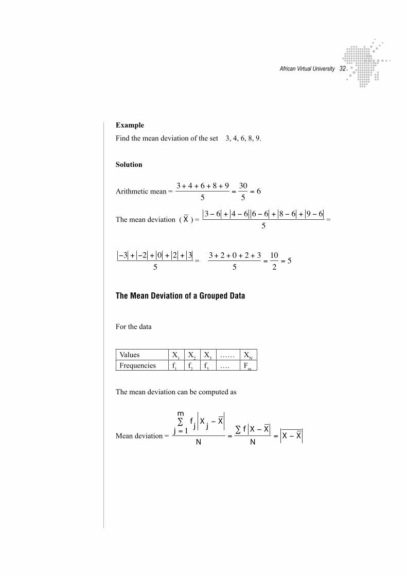
Example
Find the mean deviation of the set 3, 4, 6, 8, 9.
Solution
Arithmetic mean = 3+ 4 + 6 + 8 + 9
5=
305
= 6
The mean deviation ( X ) = 3− 6 + 4 − 6 6 − 6 + 8 − 6 + 9 − 6
5=
−3 + −2 + 0 + 2 + 35
= 3+ 2 + 0 + 2 + 3
5=
102
= 5
The Mean Deviation of a Grouped Data
For the data
Values X1
X2
X3
…… XN
Frequencies f1
f2
f3
…. Fm
The mean deviation can be computed as
Mean deviation =
f j X j − Xj = 1
m∑
N=
f X − X∑
N= X − X

African Virtual University ��
The Standard Deviation
The Standard deviation of a set of N numbers X1 ,X
2, X
3, X
4, X
5,……, X
N is denoted
by s and is defined by:
s =
(X j − X )2j = 1
N∑
N =
(X − X )2∑N
= x2∑
N= (X − X )2
where x represents the deviations of the numbers X j from the mean X .
It follows that the standard deviation is the root mean square of the deviations
from the mean.
The Standard Deviation Of A Grouped Data
Values X1
X2
X3
…… XN
Frequencies f1
f2
f3
…. Fm
The standard deviation is calculated as:
s =
f j (X − X )2j = 1
m∑
N=
f (X − X )2∑N
=fx2∑N
= (X − X )2
where N= f jj = 1
m∑ = f∑ .
The Variance
The variance of a set of data is defined as the square of the standard deviation i.e
variance = s2. We sometimes use s to denote the standard deviation of a sample of a population and σ ( Greek letter sigma ) to denote the standard deviation of a po-
pulation population. Thus σ2 can represent the variance of a population and s2 the variance of sample of a population.

African Virtual University ��
Examples
Find the Mean and Range of the following data: 5,5,4,4,4,2,2,2
Solutions
Mean = m
n∑N
x = 5 + 5 + 4 + 4 + 4 + 4 + 2 + 2 + 2
9 = 3.56
= 3.56
Range 5 – 2 =3.
Median (Middle )Observation
Example
Given 13 observations
1,1,2,3,4,4,5,6,8,10,14,15,17
The median = n+1
2=
142
= 607
The value 142
= 7th position. The median is 5
If n is odd the Median is the value in position
n+1
2
But if it is even, we consider the average of the two middle terms.
7

African Virtual University ��
10) Example
1,1,2,2,3,4,4,5,6,8,10,14,15,17
The median = Average of the Middle two terms
= 4 + 5
2= 4.5
Median of Grouped Data
When data are grouped the median c 2 is the value at or below 50% of the obser-vation fall.
DO THIS
Find the median of the following data
1. 1,1,2,2,3,4,5,7,7,7,9
2. 7,8,1,1,9,19,11,2,3,4,8
Definition
The mean squared deviation from the mean is called variance:
s2 =Σh (x − x
−
)2
N
Where: x − x−
is deviation from the mean, N is number of observations
s2 is variance and s2 is standard deviation.
qGroup Work
Study the computation of the variance and standard from the following example.

African Virtual University ��
Example
Given the data 2,4,5,8,11. Find the variance and the standard deviation.
Xx − x
−
(x − x−
)2
2 -4 164 -2 45 -1 18 2 411 5 25
x∑ =5 ∑ (x − x−
)2 =50
So x−
=305
= 6 52 =505
= 10
Variance= s2 =505
= 10Standard deviation = √10.
DO THIS
1) Calculate range of the data: 1,1,1,2,2,3,3,3,4,5
10) Calculate the variance and the standard deviation: 1,2,3,4,5
Skewness
Definition: Skewness is the degree of departure from symmetry of a distribution. ( Check positive and negative skewness above)
For skewed distributions, the mean tends to lie on the same side of the mode as the longer tail.

African Virtual University ��
Pearson’s First Coefficient of Skewness
This coefficient is defined as
Skewness=mean− mod e
s tan dard deviation=
X − mod es
Pearson’s Second Coefficient of Skewness
This coefficient is defined as:
Skewness= 3(mean− median)
s tan dard deviation=
3(X − median)s
Quartile Coefficient of Skewness
This is defined as:
Quartile coefficient of skewness = (Q3 − Q2) − (Q2 − Q1)
Q3 − Q1=
Q3 − 2Q2 + Q1Q3 − Q1
10-90 Percentile of Skewness
This is defined as:
10-90 percentile of skewness =(P90 − P50) − (P50 − P10)
P90 − P10=
P90 − 2P50 + P10P90 − P10
African Virtual University ��
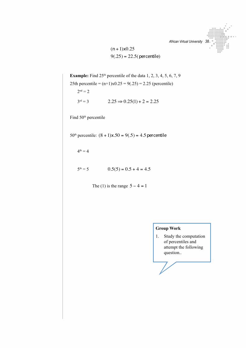
Example: Find 25th percentile of the data 1, 2, 3, 4, 5, 6, 7, 9
25th percentile = (n+1)x0.25 = 9(.25) = 2.25 (percentile)
2nd = 2
3rd = 3 2.25 ⇒ 0.25(1) + 2 = 2.25
Find 50th percentile
50th percentile: (8 +1)x.50 = 9(.5) = 4.5 percentile
4th = 4
5th = 5 0.5(5) = 0.5 + 4 = 4.5
The (1) is the range 5 − 4 = 1
qGroup Work
1. Study the computation of percentiles and attempt the following question..
(n+1)x0.259(.25) = 22.5( percentile)

African Virtual University ��
DO THIS
Find the 25th percentile, the 50th percentile, and 90th percentile
46,21,89,42,35,36,67,53,42,75,42,75,47,85,40,73,48,32,41,20,75,48,48,32,52,61, 49,50,69,59,30,40,31,25,43,52,62,50
Answer Key
a) 36 b) 48 c) 73
Kurtosis
Definition: Kurtosis is the degree of peakedness of a distribution, as compared to the normal distribution.
Eamples
1) Leptokurtic Distribution
A distribution having a relatively high peak
2) Platykurtic Distribution
A distribution having a relatively flat top

African Virtual University �0
3). Mesokurtic Distribution
A Normal Distribution – not very peaked or flat topped
DO THIS
Find the mode for the data collection:
1) 1,3,4,4,2,3,5,1,3,3,5,4,2,2,2,3,3,4,4,5
2) Number of marriage per 1000 persons in Africa population for years 1965 – 1975
Year Rate1965 9.31966 9.51967 9.71968 10.41969 10.61970 10.61971 10.61972 10.91973 10.81974 10.51975 10.0

African Virtual University ��
3) Number of deaths per 1000 years for years 1960 and 1965 – 1975
1960 9.51965 9.41966 9.51967 9.41968 9.71969 9.5 1970 9.51971 9.31972 9.41973 9.31974 9.11975 8.8
Solutions
1. 3
2. 10.6
3. 9.5
READ:
1) An Introduction to Probability by Charles M. Grinstead pages 247 -263
• Exercise on pg 263-267 Nos. 4,7,8,9

African Virtual University ��
Probability
1) Sample Space and Events
Terminology
a) A Probability experiment
When you toss a coin or pick a card from a deck of playing cards or roll a dice, the act constitutes a probability experiment. In a probability experiment, the chances are well defined with equal chances of occurrence e.g. there are only two possible chances of occurrence in tossing a coin. You either get a head or tail. The head and the tail have equal chances of occurrence.
b) An Outcome
This is defined as the result of a single trial of a probability experiment e.g. When you toss a coin once, you either get head or tail.
c) A trial
This refers to an activity of carrying out an experiment like picking a card from a deck of cards or rolling a die or dices.
d) Sample Space
This refers to all possible outcomes of a probability experiment. e.g. in tossing a coin, the outcomes are either Head(H) or tail(T) i.e there are only two possible outcomes in tossing a coin. The chances of obtaining a head or a tail are equal.
e) A Simple and Compound Events
In an experimental probability, an event with only one outcome is called a simple event. If an event has two or more outcomes, it is called a compound event.
2) Definition of Probability
Probability can be defined as the mathematics of chance. There are mainly four approaches to probability;
1) The classical or priori approach2) The relative frequency or empirical approach3) The axiomatic approach4) The personalistic approach

African Virtual University ��
The Classical or A Priori Approach
Probability is the ratio of the number of favourable cases as compared to the total likely cases. Suppose an event can occur in N ways out of a total of M possible ways. Then the probability of occurrence of the event is denoted by
p=Pr(N)=NM
. Probability refers to the ratio of possible outcomes to all possible outcomes.
The probability of non-occurrence of the same event is given by {1-p(occurrence)}. The probability of occurrence plus non-occurrence is equal to one.
If probability occurrence; p(O) and probability of non-occurrence (O’), then p(O)+p(O’)=1.
Empirical Probability ( Relative Frequency Probability)
Empirical probability arises when frequency distributions are used.
For example:
Observation ( X) 0 1 2 3 4
Frequency ( f) 3 7 10 16 11
The probability of observation (X) occurring 2 times is given by the formulae
P(2)=freuency of 2
sum of frequencies=
f (2)f∑=
103+ 7 +10 +16 +11
=1047
3) Properties of Probability
a) Probability of any event lies between 0 and 1 i.e. 0 p(O) 1. It follows that probability cannot be negative nor greater than 1.
b) Probability of an impossible event ( an event that cannot occur ) is always zero(0)
c) Probability of an event that will certainly occur is 1.d) The total sum of probabilities of all the possible outcomes in a sample space
is always equal to one(1).e) If the probability of occurrence is p(o)= A, then the probability of non-occur-
rence is 1-A.

African Virtual University ��
Counting Rules
1) Factorials
Definition: Factorial 4 ! = 4 x 3 x 2 x 1 and 7! = 7 x 6 x 5 x 4 x 3 x 2 x 1
2) Permutation Rules
Definition: nP
r =
n !(n− r ) !
Examples
•5P
3 = 5!
(5 − 3)!=
5x4x3x2x12x1
= 5x4x3 = 60
•8P
5 =
8!(8 − 5)!
=8!3!
=8x7x6x5x4x3x2x1
3x2x1= 8x7x6x5x4 = 6720
3) Combinations
Definition: nC
r =
n !(n− r ) ! r !
Examples
•5C
2 =
5!(5 − 2)!2!
=5x4x3x2x1
3! 2!=
5x42x1
= 10
•10
C6 =
10!(10 − 6)!6!
=10!
4! 6!=
10x9x8x7x 6!4x3x21x 6!
=10x9x8x74x3x2x1
= 210

African Virtual University ��
DO THIS
Work out the following;
1). 8P
3
2) 8C
3
3) 15
C10
4) 6C
3
5) 15
P4
6) 9C
3
7) 10
C8
8) 7
P4
Answer key
1) 336 2) 56 3) 3003 4) 20
5) 32 760 6)84 7)90 8) 840

African Virtual University ��
Rules of Probability
Addition Rules
1) Rule 1: When two events A and B are mutually exclusive, then
P(A or B)=P(A)+P(B)
Example: When a is tossed, find the probability of getting a 3 or 5.
Solution: P(3) =1/6 and P(5) =1/6.
Therefore P( 3 or 5) = P(3) + P(5) = 1/6+1/6 =2/6=1/3.
2) Rule 2: If A and B are two events that are NOT mutually exclusive, then
P(A or B) = P(A) + P(B) - P(A and B), where A and B means the number of outcomes that event A and B have in common.
Example: When a card is drawn from a pack of 52 cards, find the probability that the card is a 10 or a heart.
Solution
P( 10) = 4/52 and P( heart)=13/52P ( 10 that is Heart) = 1/52P( A or B) = P(A) +P(B)-P( A and B) = 4/52 _ 13/52 – 1/52 = 16/52.
Multiplication Rules
1) Rule 1: For two independent events A and B, then P( A and B) = P(A) x P(B).
Example: Determine the probability of obtaining a 5 on a die and a tail on a coin in one throw.
Solution: P( 5) =1/6 and P(T) =1/2.
P(5 and T)= P( 5) x P(T) = 1/6 x ½= 1/12.
2) Rule 2: When to events are dependent, the probability of both events occurring is P(A and B)=P(A) x P(B|A), where P(B|A) is the probability that event B occurs given that event A has already occurred.

African Virtual University ��
Example: Find the probability of obtaining two Aces from a pack of 52 cards without replacement.
Solution: P( Ace) =2/52 and P( second Ace if NO replacement) = 3/51
Therefore P(Ace and Ace) = P(Ace) x P( Second Ace) = 4/52 x 3/51 = 1/221
Conditional Probability
The conditional probability of two events A and B is P(A|B) =P (A and B)
P (B),
where P(A and B) means the probability of the outcomes that events A and B have in common.
Example: When a die is rolled once, find the probability of getting a 4 given that an even number occurred in an earlier throw.
Solution: P( 4 and an even number) = 1/6 ie. P(A and B) =1/6. P(even number) =3/6 =1/2.
P( A|B) = P (A and B)
P (B)=
16
12
=13
Examples
1) A bag contains 3 orange, 3 yellow and 2 white marbles. Three marbles are se-lected without replacement. Find the probability of selecting two yellow and a white marble.
Solution. P( 1st Y) =3/8, P( 2nd Y) = 2/7 and P( W)= 2/6
P(Y and Y and W)=P(Y) x P(Y) x P(W) = 3/8 x 2/7 x 2/6 = 1 / 28
2) In a class, there are 8 girls and 6 boys. If three students are selected at random for debating, find the probability that all girls.
Solution: P( G) =8/14 and P(B) =6/14. P( 1st G)=8/14, P(2nd G) 7/13 and P(3rdG)= 6/12.
P( three girls) 8/14 x 7/13 x 6/12= 2/13
3) In how many ways can 3 drama officials be selected from 8 members?
Solution: 8C
3 = 56 ways.

African Virtual University ��
4) A box has 12 bulbs, of which 3 are defective. If 4 bulbs are sold, find the proba-bility that exactly one will be defective.
Solution
P( defective bulb)= 3C
1 and P( non-defective bulbs) =
9C
3
3C
1 x
9C
3 =
3!(3−1)!1!
x9!
(9 − 3)!3!= 252
P( 4 bulbs from 12) = 12
C4 = 495.
P( 1 defective bulb and 3 okey bulbs) = 295/495=0.509.
DO THIS
1) In how many ways can 7 dresses be displayed in a row on a shelf?2) In how many ways can 3 pens be selected from 12 pens?3) From a pack of 52 cards, 3 cards are selected. What is the probability that
they will all be diamonds?
Answer Key
1) 5040
2) 220
3) 0.013

African Virtual University ��
READ:
An Introduction to Probability & Random Processes By Kenneth B & Gian-Carlo R, pages1. 1.20 -1.22
• Exercise Chapter 1: Sets, Events & Probability Pg 1.23-1.28 Nos. 1-12 & 14-20
2. 2.1-2.33• Exercise Chapter 2: Finite Pro-
cesses Pg 2.33 Nos. 1,2,3,13-20, 22-27
3. Introduction to Probability, By Charles M. Grinstead pages139-141
Random Variables
Random Variables ( r.v)
Definition: A random variable is a function that assigns a real number to every pos-sible result of a random experiment.
(Harry Frank & Steve C Althoen,CUP, 1994, pg 155)
A random variable is a variable in the sense that it can be used as a placeholder for a number in equations and inequalities. Its randomness is completely described by its cumulative distribution function which can be used to determine the probability it takes on particular values.
Formally, a random variable is a measurable function from a probability space to the real numbers. For example, a random variable can be used to describe the process of rolling a fair die and the possible outcomes { 1, 2, 3, 4, 5, 6 }. The most obvious representation is to take this set as the sample space, the probability measure to be uniform measure, and the function to be the identity function.
Random variable
Some consider the expression random variable a misnomer, as a random variable is not a variable but rather a function that maps outcomes (of an experiment) to numbers. Let A be a σ-algebra and Ω the space of outcomes relevant to the experiment being performed. In the die-rolling example, the space of outcomes is the set Ω = { 1, 2, 3, 4, 5, 6 }, and A would be the power set of Ω. In this case, an appropriate random

African Virtual University �0
variable might be the identity function X(ω) = ω, such that if the outcome is a ‘1’, then the random variable is also equal to 1. An equally simple but less trivial example is one in which we might toss a coin: a suitable space of possible outcomes is Ω = { H, T } (for heads and tails), and A equal again to the power set of Ω. One among the many possible random variables defined on this space is
Mathematically, a random variable is defined as a measurable function from a sample space to some measurable space.
Convergence of Random Variables
In probability theory, there are several notions of convergence for random variables. They are listed below in the order of strength, i.e., any subsequent notion convergence in the list implies convergence according to all of the preceding notions.
Convergence in distribution: As the name implies, a sequence of random variables
converges to the random variable in distribution if their res-
pective cumulative distribution functions converge to the cumulative distribution function of , wherever is continuous.
Weak convergence: The sequence of random variables is said to conver-
ge towards the random variable weakly if for every ε > 0. Weak convergence is also called convergence in probability.
Strong convergence: The sequence of random variables is said to
converge towards the random variable strongly if Strong convergence is also known as almost sure convergence.
Intuitively, strong convergence is a stronger version of the weak convergence, and
in both cases the random variables show an increasing correlation with . However, in case of convergence in distribution, the realized values of the random variables do not need to converge, and any possible correlation among them is immaterial.

African Virtual University ��
Law of Large Numbers
If a fair coin is tossed, we know that roughly half of the time it will turn up heads, and the other half it will turn up tails. It also seems that the more we toss it, the more likely it is that the ratio of heads:tails will approach 1:1. Modern probability allows us to formally arrive at the same result, dubbed the law of large numbers. This result is remarkable because it was nowhere assumed while building the theory and is completely an offshoot of the theory. Linking theoretically-derived probabilities to their actual frequency of occurrence in the real world, this result is considered as a pillar in the history of statistical theory.
The strong law of large numbers (SLLN) states that if an event of probability p is observed repeatedly during independent experiments, the ratio of the observed fre-quency of that event to the total number of repetitions converges towards p strongly in probability.
In other words, if are independent Bernoulli random variables taking values 1 with probability p and 0 with probability 1-p, then the sequence of random
numbers converges to p almost surely, i.e.
Central Limit Theorem
The central limit theorem is the reason for the ubiquitous occurrence of the normal distribution in nature, for which it is one of the most celebrated theorems in proba-bility and statistics.
The theorem states that the average of many independent and identically distributed random variables tends towards a normal distribution irrespective of which distribution
the original random variables follow. Formally, let be independent
random variables with means , and variances Then the sequence of random variables
converges in distribution to a standard normal random variable.

African Virtual University ��
Functions of Random Variables
If we have a random variable X on Ω and a measurable function f: R → R, then Y = f(X) will also be a random variable on Ω, since the composition of measurable functions is also measurable. The same procedure that allowed one to go from a probability space (Ω, P) to (R, dF
X) can be used to obtain the distribution of Y. The
cumulative distribution function of Y is
Example
Let X be a real-valued, continuous random variable and let Y = X2. Then,
If y < 0, then P(X2 ≤ y) = 0, so
If y ≥ 0, then
So
Probability Distributions
Certain random variables occur very often in probability theory due to many natural and physical processes. Their distributions therefore have gained special importance in probability theory. Some fundamental discrete distributions are the discrete uniform, Bernoulli, binomial, negative binomial, Poisson and geometric distributions. Impor-tant continuous distributions include the continuous uniform, normal, exponential, gamma and beta distributions.
Distribution Functions
If a random variable defined on the probability space (Ω,A,P) is given, we can ask questions like “How likely is it that the value of X is bigger than 2?”.
This is the same as the probability of the event which is often written as P(X > 2) for short.
Recording all these probabilities of output ranges of a real-valued random variable X

African Virtual University ��
yields the probability distribution of X. The probability distribution “forgets” about the particular probability space used to define X and only records the probabilities of various values of X. Such a probability distribution can always be captured by its cumulative distribution function
and sometimes also using a probability density function. In measure-theoretic terms, we use the random variable X to “push-forward” the measure P on Ω to a measure dF on R. The underlying probability space Ω is a technical device used to guarantee the existence of random variables, and sometimes to construct them. In practice, one often disposes of the space Ω altogether and just puts a measure on R that assigns measure 1 to the whole real line, i.e., one works with probability distributions instead of random variables.
Discrete Probability Theory
Discrete probability theory deals with events which occur in countable sample spaces.
Examples: Throwing dice, experiments with decks of cards, and random walk.
Classical definition: Initially the probability of an event to occur was defined as num-ber of cases favorable for the event, over the number of total outcomes possible.
For example, if the event is “occurrence of an even number when a die is rolled”, the
probability is given by , since 3 faces out of the 6 have even numbers.
Modern definition: The modern definition starts with a set called the sample space which relates to the set of all possible outcomes in classical sense, denoted by
. It is then assumed that for each element , an intrinsic
“probability” value is attached, which satisfies the following properties:
1.
2.
An event is defined as any subset of the sample space . The probability of the event defined as
So, the probability of the entire sample space is 1, and the probability of the null event is 0.

African Virtual University ��
The function mapping a point in the sample space to the “probability” value is called a probability mass function abbreviated as pmf. The modern definition does not try to answer how probability mass functions are obtained; instead it builds a theory that assumes their existence.
Continuous Probability Theory
Continuous probability theory deals with events which occur in a continuous sample space.
If the sample space is the real numbers, then a function called the cumulative distri-
bution function or cdf is assumed to exist, which gives .
The cdf must satisfy the following properties.
1. is a monotonically non-decreasing right-continuous function
2.
3.
If is differentiable, then the random variable is said to have a probability density
function or pdf or simply density .
For a set , the probability of the random variable being in is defined as
In case the density exists, then it can be written as
Whereas the pdf exists only for continuous random variables, the cdf exists for all random variables (including discrete random variables) that take values on .
These concepts can be generalized for multidimensional cases on .

African Virtual University ��
Probability Density Function
Discrete Distribution
If X is a variable that can assume a discrete set of values X1, X
2, X
3,…….., X
k wih
respet to probabilities p1, p
2, p
3,……., p
k, where p
1+ p
2 + p
3,……., + p
k = 1, we say
that a discrete probability distribution for X has been defined. The function p(X), which has the respective values p
1, p
2, p
3,……., p
k for X= X
1, X
2, X
3,…….., X
k is
called the probability function, or frequency function, of X. Because X can assume certain values with given probabilities, it is often called a discrete random variable. A random variable is also known as a chance variable or stochastic variable. { Murray R, 2006 pg 130}
Continuous Distribution
Suppose X is a continuous random variable. A continuous random variable X is speci-fied by its probability density function which is written f(x) where f(x)≥ 0 throughout the range of values for which x is valid. This probability density function can be represented by a curve, and the probabilities are given by the area under the curve.
The total area under the curve is equal to 1. The are under the curve between the lines x=a and x=b ( shaded) gives the probability that X lies between a and b, which can be denoted by P(a<X<b). p(X) is called a probability density function and the variable X is often called a continuous random variable
Since the total area under the curve is equal to 1, it follows that the probability between a range space a and b is given by
P (a ≤ X ≤ b) = f (x)a
b∫ dx ,
which is the shaded area.

African Virtual University ��
Note: when computing area from a to b, we need not dist inguish
(≤ and ≥) and (< and >) inequalities. We assume the lines at a and b have no thickness and its area is zero.
Solved Examples
1) The continuous random variable X is distributed with probability density function f defined by
f(x) = kx(16-x2), for 0<x<4.
Evaluate
a). The value of constant kb). The probability of range space P(1<X<2)
c). The probability P(x≥ 3)
Solution
a b
x
f(x)
For any function f(x) such tha
f(x) ≥ 0, for a ≤ x ≤ b,
and f (x)dx = 1ab∫
may be taken as the probability density function (p.d.f) of a continuous random va-riable in the range space a ≤ x ≤ b.

African Virtual University ��
Procedure
Step 1: In general, if X is a continuous random variable (r.v) with p.d.f f(x) valid
over the range a ≤ x ≤ b, then
f (x)dx = 1all x∫ i.e.
f (x)dx = 1
a
b
∫
Step 2
a). To determine k, we use the fact that in f(x) = kx(16-x2), for 0<x<4, then
kx(16 − x2 )dx = 1
0
4
∫
⇒ k 16x − x3 )dx = 1
0
4
∫
⇒ k =1
64Step 3
b). Find P(1<X<2)
Solution
P(1<X<2)= f (x)dx1
2
∫
=
164
(16x − x3
1
2
∫ )dx =81
256
Step 4
c). To find P(x≥ 3)
P (x ≥ 3) = 1
64(16x − x3
3
4
∫ )dx =49
256

African Virtual University ��
Example 2
2). X is the continuous random variable ‘the mass of a substance, in kg, per minute in an industrial production process’, where
f (x) =1
12x(6 − x)
0
⎧
⎨⎪
⎩⎪
(0 ≤ x ≤ 3)otherwise
Find the probability that the mass is more than 2 kg.
Solution
X can take values from 0 to 3 only. We sketch f(x), and shade the area required.
0 3
x
f(x) )6(121
)( xxxf −=
2
P (x > 2) = 1122
3
∫ x(6 − x)dx
=1
12(6x − x2
2
3
∫ )dx
=1
123x2 −
x3
3⎡
⎣⎢
⎤
⎦⎥
2
3
= 0.722 (3 d.p)
The probability that the mass is more than 2 kg is 0.722.

African Virtual University ��
Worked example
3). A continuous random variable has p.d.f f(x) where
f (x) = kx2 , 0 ≤ x ≤ 6. a). Find the value of k
b). Find P (2 ≤ X ≤ 4)
Solution
a). Since X is a random variable the total probability is 1. i.e.
f (x)dx = 1all∫
⇒ kx2
0
6
∫ dx = 1
kx3
3⎡
⎣⎢
⎤
⎦⎥
0
6
= = 1
216k3
= 1
⇒ k =3
216
Therefore f(x)=3
216x2 =
172
x2 , 0 ≤ x ≤ 6
b).
0 6
x
f(x)
4 2
2
721
)( xxf =
African Virtual University �0
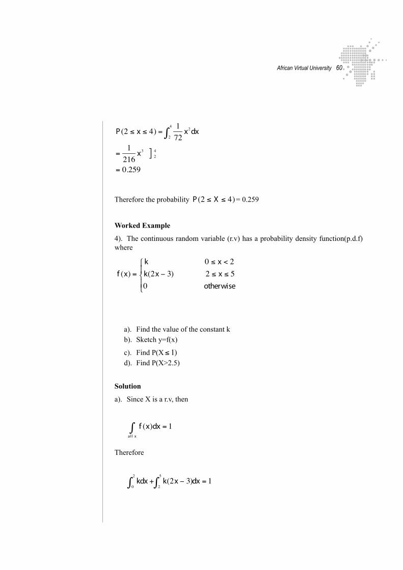
P (2 ≤ x ≤ 4) = 172
x2 dx2
4
∫
=1
216x3 ] 2
4
= 0.259
Therefore the probability P (2 ≤ X ≤ 4) = 0.259
Worked Example
4). The continuous random variable (r.v) has a probability density function(p.d.f) where
f (x) =k 0 ≤ x < 2k(2x − 3) 2 ≤ x ≤ 50 otherwise
⎧
⎨⎪
⎩⎪
a). Find the value of the constant kb). Sketch y=f(x)
c). Find P(X≤ 1)d). Find P(X>2.5)
Solution
a). Since X is a r.v, then
f (x)dx = 1all x∫
Therefore
kdx +
0
2
∫ k(2x − 3)2
5
∫ dx = 1

African Virtual University ��
kx0
2+ k x2 − 3x⎡⎣ ⎤⎦2
5
2k +19k = 1
⇒ k =121
b). So the p.d.f of X is
f (x) =
121
0 ≤ x < 2
121
(2x − 3) 2 ≤ x ≤ 5
0 otherwise
⎧
⎨
⎪⎪⎪⎪⎪
⎩
⎪⎪⎪⎪⎪
Sketch
2 5
0
3
1
1 3 4 2.5
211

African Virtual University ��
c). P(x≤ 1)= area between zero and 1 = L x W= 1 x 121
=121
= 0.048
d). Find P(X>2.5) = area of rectangle + area of trapezium.
=( 121
x 2 ) + (12
{0.5}{ 121
+221
} =1184
= 0.131

African Virtual University ��
qReflection : Teachers may find graph drawing software useful in the teaching of statistics.
An example of Open Source software is Graph. See: http://www.padowan.dk/graph/
If you have computer access, download graph and explore its statis-tical features.
Here is an example of different trendlines which can be drawn using Graph.

African Virtual University ��
DO THIS
1). The continuous random variable X has p.d.f f(x) where f(x)= k, 0≤ x ≥ 3 .
a) Sketch y=f(x)
b). Find the value of the constant k
c). Find P(0.5≤ X ≤ 1
2). The continuous random variable has p.d.f f(x) where f(x)=kx2,1 ≤ x ≤ 4 .
a). Find the value of the constant
b). Find P(x≥ 2)
c). Find P(2.5≤ x ≤ 3.53). The continuous random variable has p.d.f f(x) where
f (x)k 0 ≤ x < 2k(2x −1) 2 ≤ x ≤ 30 otherwise
⎧
⎨⎪
⎩⎪
a) find the value of the constant k.
b) Sketch y=f(x)
c) Find P(X≤ 2 )
d) Find P(1≤ X ≤ 2.2)

African Virtual University ��
Expectation
Definition
If X is a continuous variable (r.v) with probability density function (p.d.f) f(x), then the expectation of X is E(X) where
E (X ) = x f (x)dxall x∫
NB: E(X) is often denoted by μ and referred to as the mean of X
Example
1). If X is a continuous variable ( r.v) with a p.d.f f (x) = 116
x2 , 0 ≤ x ≤ 3 , find E(X).
Solution
E (X ) = x f (x)dxall x∫
⇒1
160
3
∫ {x} x2 dx
=1
16x4
4⎡
⎣⎢
⎤
⎦⎥
0
3
=8164
= 1.265
2). If the continuous random variable X has p.d.f
f (x) = 25
(3+ x)(x −1), 1 ≤ x ≤ 3 , find E(X).
E (X ) = x f (x)dxall x∫

African Virtual University ��
E (x) = 251
3
∫ {x} (3+ x)(x −1)dx
=25
x4
4+
2x3
3−
3x2
2⎡
⎣⎢
⎤
⎦⎥
1
3
=60860
= 10.13
Generalisation
If g( x) is any function of the continuous random variable r.v X having p.d.f f(x), then
E g(X )[ ] = g(x) f (x)dxall x∫
and in particular
E (X 2 ) = x2
all x∫ f x( )dx
The following conclusions hold1. E (a) = a2. E (aX ) = aE (X )3. E (aX + b) = aE (X ) + b
4. E ( f1 (X ) + f2 (X )[ ] = E f2 (X )[ ]
Example
1). The continuous random variable X has p.d.f f(x) where f(x)= 12
x, 0 ≤ x ≤ 3.
Find
a). E(X)
b). E(X2)
c). E(2X +3)

African Virtual University ��
Solution
a) E (X ) = x f (x)dxall x∫
=120
3
∫ x2 dx
=12
x3
3⎡
⎣⎢
⎤
⎦⎥
0
3
= 4.5
b)
E (X 2 ) = x2
all x∫ f (x)dx
=12
x3dx0
3
∫
=12
x4
4⎡
⎣⎢
⎤
⎦⎥
0
3
=818
= 10.125
c). E(2X +3) = E (2X) + 3
= 2E(X) +3
= 2(10.125)+5
= 25.25 ( from (b) above)

African Virtual University ��
DO THIS
1) The continuous random variable X has p.d.f f(x) where
f (x) =kx 0 ≤ x < 1
k 1 ≤ x < 3k(4 − x) 3 ≤ x ≤ 50 otherwise
⎧
⎨
⎪⎪⎪
⎩
⎪⎪⎪
a). Find kb). Calculate E(X)
2) The continuous random variable has p.d.f f(x) where f(x) = 110
(x + 3), 0 ≤ x ≤ 5
a). Find E(X)b). Find E(2X+4)c). Find E(X2).d). Find E( X2 + 2X – 1).

African Virtual University ��
Bernoulli Distribution
In probability theory and statistics, the Bernoulli distribution, named after Swiss scientist Jakob Bernoulli, is a discrete probability distribution, which takes value 1 with success probability p and value 0 with failure probability q = 1 − p. So if X is a random variable with this distribution, we have:
The probability mass function f of this distribution is
The expected value of a Bernoulli random variable X is , and its va-riance is
The kurtosis goes to infinity for high and low values of p, but for p = 1 / 2 the Bernoulli distribution has a lower kurtosis than any other probability distribution, namely -2.
The Bernoulli distribution is a member of the exponential family.
Binomial Distribution
In probability theory and statistics, the binomial distribution is the discrete proba-bility distribution of the number of successes in a sequence of n independent yes/no experiments, each of which yields success with probability p. Such a success/failure experiment is also called a Bernoulli experiment or Bernoulli trial. In fact, when n = 1, the binomial distribution is a Bernoulli distribution. The binomial distribution is the basis for the popular binomial test of statistical significance.
Examples
An elementary example is this: roll a die ten times and count the number of 1s as outcome. Then this random number follows a binomial distribution with n = 10 and p = 1/6.
For example, assume 5% of the population is green-eyed. You pick 500 people randomly. The number of green-eyed people you pick is a random variable X which follows a binomial distribution with n = 500 and p = 0.05 (when picking the people with replacement).

African Virtual University �0
Examples
1) A coin is tossed 3 times. Find the probability of getting 2 heads and a tail in any given order.
Formula
We can use the formula nC
x. (p)x.(1-p)n-x
Where n = the total number of trials
x = the number of successes ( 1,2,…)
p= the probability of a success.
1st) nC
x determines the number of ways a success can occur.
2nd) (p)x is the probability of getting x successes and
3rd) (1-p)n-x is the probability of getting n-x failures
Solution
Tossing 3 times means n=3
Two heads means x=2
P(H)=1/2; P(T)=1/2
P( 2 heads) = 3C
2. (
12
)2.(1-12
)3-1 = 3(1/4)(1/2)= 3/8

African Virtual University ��
DO THIS
1) Find the probability of exactly one 5 when a die is rolled 3 times
2) Find the probability of getting 3 heads when 8 coins are tossed.
3) A bag contains 4 red and 2 green balls. A ball is drawn and replaced 4 times. What is the probability of getting exactly 3 red balls and 1 green ball.
Answer
1). P( one 5) = 3C
1. (
16
)1.(56
)2 = 25/72 = 0.347 i.e n=3, x=1, p=1/6
2). P ( 3 heads) = 8C
3. (
12
)3.(12
)5 = 7/32 = 0.218. i.e n=8, x=3, p=1/2
3). P( 3 Red balls) = 4C
3. (
23
)3.(13
)1 = 32/81= 0.395 i.e. n=4, x=3, p=2/3
READ:
1. Lectures on Statistics, By Robert B. Ash, , page 1-4• Exercise Nos.1, 2 and 3 on pg 4.
2. An Introduction to Probability & Random Processes By Kenneth B & Gian-Carlo R, pages 3.1-3.63
• Exercise Chapter 3: Random Variables pg 3.64-3.82 Nos. 1-7, 11-17, 20-24, 34-36
3. An Introduction to Probability By Charles M. Grinstead pages 96-107, & 184
• Exercise on pages 113-118 Nos. 1,2,3,4,5,8,9,10,19,20
Ref: http://en.wikipedia.org/wiki/measurable_spaceRef: http://en.wikipedia.org/wiki/Probability_theoryRef: http://en.wikipedia.org/wiki/Bernoulli_distribution

African Virtual University ��
Poisson Distribution
In probability theory and statistics, the Poisson distribution is a discrete probability distribution that expresses the probability of a number of events occurring in a fixed period of time if these events occur with a known average rate, and are independent of the time since the last event.
The distribution was discovered by Siméon-Denis Poisson (1781–1840)
The Poisson distribution is sometimes called a Poissonian, analagous to the term Gaussian for a Gauss or normal distribution.
The Poisson distribution is used when the variable occurs over a period of time, volume, area etc…it can be used for the arrival of airplanes at airports, the number of phone calls per hour for a station, the number of white blood cells on a certain area.
The probability of x successes is
e− λλ x
x!where e is a mathematical constant = 2.7183
λ is the mean or expected value of the variables.
Example
If there are 100 typographical errors randomly distributed. In 500 pages manuscripts find the probability that any given page has exactly 4 errors.
Solution
Find the mean number of errors λ = 100/500 = 1 / 5 = 0,2
In other words there is an average of 0.2 errors per page. In this case λ = 4 so the probability of selecting a page with exactly 4 errors
eλ.λ x
x!=
2.7183( )−0.2 0.2( )4
41
= 0.00168
Amount 0.2%
qGroup Work
1. Study the probability computations and attempt the given question.

African Virtual University ��
Worked Example
A hot line with a full free number receives an average of 4 calls per hour for any given hour. Find the probability that it will receive exactly 5 calls.
eλ.λ x
x!=
2.7183( )−3 3( )5
5!
= 0.1001
Which is 10%
DO THIS
1) A telephone Marketing Company gets an average of 5 orders per 1000 calls. If a company calls 500 people find the probability of getting 2 orders.
Solution
0.26
Which is 26%
READ:
1. An Introduction to Probability & Random Processes By Kenneth B & Gian-Carlo R, pages187-192
2. Robert B. Ash, Lectures on Statistics, page 1 and Answer problems 1,2,3 on pg 15.
Ref: http://en.wikipedia.org/wiki/Normal_distribution

African Virtual University ��
Geometric Distribution
In probability theory and statistics, the geometric distribution is either of two dis-crete probability distributions:
• the probability distribution of the number X of Bernoulli trials needed to get one success, supported on the set { 1, 2, 3, ...}, or
• the probability distribution of the number Y = X − 1 of failures before the first success, supported on the set { 0, 1, 2, 3, ... }.
Which of these one calls “the” geometric distribution is a matter of convention and convenience.
If the probability of success on each trial is p1, then the probability that k trials are
needed to get one success is
for k = 1, 2, 3, ....
Equivalently, if the probability of success on each trial is p0, then the probability that
there are k failures before the first success is
for k = 0, 1, 2, 3, ....
In either case, the sequence of probabilities is a geometric sequence.
For example, suppose an ordinary die is thrown repeatedly until the first time a “1” appears. The probability distribution of the number of times it is thrown is supported on the infinite set { 1, 2, 3, ... } and is a geometric distribution with p
1 = 1/6.
Solutions Using The Geometric Distribution Formula
The formula for the probability that the first success occurs on the nth trial is
(1-p)n-1p or simply , where p is the probability of a success and n is the trial number of the first success.
Example
1) Find the probability that the first tail occurs on the third toss of a coin.
Solution
The outcome of a tail on the third throw implies HHT. From (1-p)n-1p , n=3, p=1/2
and therefore P(HHT) = ( 1-12
)3-1 (12
) = (12
) .. (12
) (12
) =1/8

African Virtual University ��
Examples In Geometric Distribution
Flipping a coin several times we apply the geometric to distribution to get the answer of flipping a coin several times.
Example
1) A coin is tossed find the probability that the first head occurs on the third toss solution. Out come is TTH
n = 3 and p=1/2
Probability of getting 2 tails and then one head is
12−
12−
12=
18
Or by the formula
1− 12
⎛⎝⎜
⎞⎠⎟
3−1
. 12=
12
⎛⎝⎜
⎞⎠⎟
2 12
⎛⎝⎜
⎞⎠⎟=
18
.
2) A die is rolled; find the probability of getting the first 3 on the fourth roll.
Solution
n=4 p=1/6
∴ 1− 1
6⎛⎝⎜
⎞⎠⎟
4 −1 16
⎛⎝⎜
⎞⎠⎟=
56
⎛⎝⎜
⎞⎠⎟
3 56
⎛⎝⎜
⎞⎠⎟
3 16
⎛⎝⎜
⎞⎠⎟=
1251296
= 0.96
Example
If cards are selected from a deck and replaced, how many trials would it take on average to get two clubs?
P (Club) = 13/52=1/4
Expected no. of trials for selecting 2 clubs would be 214
= 2x41= 8
African Virtual University ��
DO THIS
1. A card from an ordinary deck of cards is selected and then replaced with another card selected etc… find the probability that the first club will occur on he fourth draw.
2. A die is tossed until 5 or 6 is obtained. Find the expected number of tosses.
Answer Key
1) Fourth
2) 3
Hypergeometric Distribution
In probability theory and statistics, the hypergeometric distribution is a discrete probability distribution that describes the number of successes in a sequence of n draws from a finite population without replacement.
A typical example is illustrated by the contingency table above: there is a shipment of N objects in which D are defective. The hypergeometric distribution describes the probability that in a sample of n distinctive objects drawn from the shipment exactly k objects are defective.
In general, if a random variable X follows the hypergeometric distribution with para-meters N, D and n, then the probability of getting exactly k successes is given by
The probability is positive when k is between max{ 0, D + n− N } and min{ n, D }.
The formula can be understood as follows: There are possible samples (without
replacement). There are ways to obtain k defective objects and

African Virtual University ��
there are ways to fill out the rest of the sample with non-defective objects.
When the population size is large compared to the sample size (i.e., N is much larger than n) the hypergeometric distribution is approximated reasonably well by a bino-mial distribution with parameters n (number of trials) and p = D / N (probability of success in a single trial).
Hypergeometric Formula
When there are two groups of items such that there are ‘a’ items in the first group and ‘b’ items in the second group, so that the total number of items is (a + b), the probability of selecting x items from the first group and (n-x) items from the second group is
a C x . bCn− x
a + bCn, where n is the total of items selected without replacement.
Examples
1. A bag contains 3 blue chips and 3 green chips. If two chips are selected at ran-dom, find the probability that both are blue.
Solution
From the formula a C x . bCn− x
a + bCn ; a = 3, b= 3, x=2, n=2, n-x=2-2=0
The probability of both blue = 3C2 . 3C2 − 2
3+ 3C2=
3 x 115
=15= 0.2
2. A committee of 3 people is selected at random without replacement from a group of 6 men and 3 women. Find the probability that the committee consists of 2 men and 2 women.
Solution
So into
a=6 b=3 n = 6+3=9

African Virtual University ��
since the committee consists 2 men and 2 women
x=2 n-.x= 3-2=1
Pr = 6C 2 3C1
9C 3
=15x3
84=
1528
= 0.536
3. A group of 10 tanks contains 3 defective tanks. If 4 tanks are randomly selected and tested find the probability that exactly one will be defective solution.
3 are defective 7 are good a=3 b=7
Pr (one to be defective) n = 4 x=1 n-x=4-1=3
Pr (one to be exactly defective)
3C1 .7C 3
10C 4
=105210
= 0.5
DO THIS
1. In a box of 10 shirts there are five (5) defective ones. If 5 shirts are sold at random find the probability that exactly two are defective. Answer
2. In a shipment of 12 lawn chairs 86 are brown and 4 are blue. If 3 chairs are sold at random find the probability that that all are brown.
Answer Key
1). 0.397 2) 0.255
qGroup Work
1. Revise the following probability questions and answers
2. Discuss any problems encountered in the computations of the probabilities.

African Virtual University ��
1) Find the probability of choosing 5 women from a committee of 15 women
P(choosing 5) = 1
15C 5
=1
3003
2) What is the probability of drawing an ace or a spade from deck of playing cards?
P (Ace) = 452
∴P AUB( ) = P A( ) + P B( ) − P AUB( )
P spade( ) = 1352
= 452
+1352
−152
= 1652
=4
13
3) There are problems pregnant for women. The probability of dying is 15
what is the probability that at least one will die in every 5 women
P A( ) = 151
P(At least one will die) 5051
⎛⎝⎜
⎞⎠⎟
5
= use calculator
P A( )1− 151
=5051
Application and Example
The classical application of the hypergeometric distribution is sampling wi-thout replacement. Think of an urn with two types of marbles, black ones and white ones. Define drawing a white marble as a success and drawing a black marble as a failure (analogous to the binomial distribution). If the varia-ble N describes the number of all marbles in the urn (see contingency table above) and D describes the number of white marbles (called defective in the example above), then N − D corresponds to the number of black marbles. Now, assume that there are 5 white and 45 black marbles in the urn. Standing next to the urn, you close your eyes and draw 10 marbles without replacement. What’s the probability p (k=4) that you draw exactly 4 white marbles (and - of course - 6 black marbles) ?

African Virtual University �0
This problem is summarized by the following contingency table:
drawn not drawn totalwhite marbles
4 (k) 1 = 5 − 4 (D − k) 5 (D)
black marbles
6 = 10 − 4 (n − k) 39 = 50 + 4 − 10 − 5 (N + k− n − D) 45 (N− D)
total 10 (n) 40 (N − n) 50 (N)
The probability Pr (k = x) of drawing exactly x white marbles (= number of successes) can be calculated by the formula
Hence, in this example x = 4, calculate
So, the probability of drawing exactly 4 white marbles is quite low (approximately 0.004) and the event is very unlikely. It means, if you repeated your random expe-riment (drawing 10 marbles from the urn of 50 marbles without replacement) 1000 times you just would expect to obtain such a result 4 times.
But what about the probability of drawing even (all) 5 white marbles? You will in-tuitively agree upon that this is even more unlikely than drawing 4 white marbles. Let us calculate the probability for such an extreme event.
The contingency table is as follows:
drawn not drawn total
white marbles 5 (k) 0 = 5 − 5 (D − k) 5 (D)
black marbles 5 = 10 − 5 (n − k) 40 = 50 + 5 − 10 − 5 (N + k − n − D) 45 (N − D)
total 10 (n) 40 (N − n) 50 (N)
And we can calculate the probability as follows (notice that the denominator always stays the same):

African Virtual University ��
As expected, the probability of drawing 5 white marbles is even much lower than drawing 4 white marbles.
Conclusion
Consequently, one could expand the initial question as follows: If you draw 10 mar-bles from an urn (containing 5 white and 45 black marbles), what’s the probability of drawing at least 4 white marbles? Or, what’s the probability of drawing 4 white marbles and more extreme outcomes such as drawing 5)? This corresponds to calcu-lating the cumulative probability p(k>=4) and can be calculated by the cumulative distribution function (cdf). Since the hypergeometric distribution is a discrete probability distribution the cumulative probability can be calculated easily by adding all corresponding single probability values.
In our example you just have to sum-up Pr (k = 4) and Pr (k = 5):
Pr (k ≥ 4) = 0.003964583 + 0.0001189375 = 0.004083520
READ:
1. An Introduction to Probability & Random Processes By Kenneth B & Gian-Carlo R, pages 184-195

African Virtual University ��
Bivariate Frequency Distributions
The bivariate normal distribution is the statistical distribution with probability func-tion
where
and
is the correlation of and (Kenney and Keeping 1951, pp. 92 and 202-205; Whit-
taker and Robinson 1967, p. 32)
are commonly used in place of and .
The marginal probabilities are then
= =

African Virtual University ��
And
= =
Joint Probability Tables
This table is a correctly formatted joint probability table.
Days Listed Until Sold
Initial Asking Price Under 30 31-90 Over 90 Totals
Under $50,000 0.06 0.05 0.01 0.13
$50,000-99,999 0.03 0.19 0.10 0.31
$100,000-150,000 0.03 0.35 0.13 0.50
Over $150,000 0.01 0.04 0.01 0.06
Totals 0.13 0.63 0.25 1.00
Marginal Probabilities
Let be partitioned into disjoint sets and where the general subset is
denoted . Then the marginal probability of is
READ:
1. An Introduction to Probability & Random Processes By Kenneth B & Gian-Carlo R, pages 142-150
2. Exercise pg 150 Nos. 1,23,4,5,6,7,8,9,14,15,16,17,26.

African Virtual University ��
qREFLECTION: ICT resources are difficult
to access!! The link opens up avenue for Mathematics teachers to access ICT resources.
http://www.tsm-resources.com/suppl.html

African Virtual University ��
Unit 2 ( 40 Hours)
Random Variables And Test Distributions
Moments
The probability distribution of a random variable is often characterised by a small number of parameters, which also have a practical interpretation. For example, it is often enough to know what its “average value” is. This is captured by the mathematical concept of expected value of a random variable, denoted E[X]. Note that in general, E[f(X)] is not the same as f(E[X]). Once the “average value” is known, one could then ask how far from this average value the values of X typically are, a question that is answered by the variance and standard deviation of a random variable.
Mathematically, this is known as the (generalised) problem of moments: for a given class of random variables X, find a collection {f
i} of functions such that the expectation
values E[fi(X)] fully characterize the distribution of the random variable X.
Equivalence of random variables
There are several different senses in which random variables can be considered to be equivalent. Two random variables can be equal, equal almost surely, equal in mean, or equal in distribution.
In increasing order of strength, the precise definition of these notions of equivalence is given below.
Equality in distribution
Two random variables X and Y are equal in distribution if they have the same dis-tribution functions:
Two random variables having equal moment generating functions have the same distribution.
Equality in mean
Two random variables X and Y are equal in p-th mean if the pth moment of |X − Y| is zero, that is,

African Virtual University ��
Equality in pth mean implies equality in qth mean for all q<p. As in the previous case, there is a related distance between the random variables, namely
Equality
Finally, the two random variables X and Y are equal if they are equal as functions on their probability space, that is,
Moment-generating Function
In probability theory and statistics, the moment-generating function of a random variable X is
wherever this expectation exists. The moment-generating function generates the moments of the probability distribution.
For vector-valued random variables X with real components, the moment-generating function is given by
where t is a vector and is the dot product.
Provided the moment-generating function exists in an interval around t = 0, the nth moment is given by
If X has a continuous probability density function f(x) then the moment generating function is given by

African Virtual University ��
where mi is the ith moment. M
X( − t) is just the two-sided Laplace transform of f(x).
Regardless of whether the probability distribution is continuous or not, the moment-generating function is given by the Riemann-Stieltjes integral
where F is the cumulative distribution function.
If X1, X
2, ..., X
n is a sequence of independent (and not necessarily identically distri-
buted) random variables, and
where the ai are constants, then the probability density function for S
n is the convolu-
tion of the probability density functions of each of the Xi and the moment-generating
function for Sn is given by
Related to the moment-generating function are a number of other transforms that are common in probability theory, including the characteristic function and the proba-bility-generating function.
Markov’s Inequality
f(x)
ε
}{ εε ≥)(| xfXX
Markov’s inequality gives an upper bound for the probability that X lies within
XεX | f (x) ≥ ε }{

African Virtual University ��
In probability theory, Markov’s inequality gives an upper bound for the probability that a non-negative function of a random variable is greater than or equal to some po-sitive constant. It is named after the Russian mathematician Andrey Markov, although it appeared earlier in the work of Pafnuty Chebyshev (Markov’s teacher).
Markov’s inequality (and other similar inequalities) relate probabilities to expectations, and provide (frequently) loose but still useful bounds for the cumulative distribution function of a random variable.
Special case: probability theory
For any event E, let IE be the indicator random variable of E, that is, I
E = 1 if E occurs
and = 0 otherwise. Thus I(|X| ≥ a)
= 1 if the event |X| ≥ a occurs, and I(|X| ≥ a)
= 0 if |X| < a. Then, given a>0,
Therefore
Now observe that the left side of this inequality is the same as
Thus we have
and since a > 0, we can divide both sides by a.
READ:
1. Robert B. Ash, Lectures on Statistics, page 9-13 2. An Introduction to Probability & Random Processes
By Kenneth B & Gian-Carlo R, pages 366 -374 & 404 - 407• Exercise on pg 376 -376 Nos. 1,3,7,8• Exercise on pg 442 Nos. 1,2,3,4,5
Ref: • http://en.wikipedia.org/wiki/Moment-generating_
function• http://en.wikipedia.org/wiki/characteristic_function_
%28probability_theory%29. • http://en.wikipedia.org/wiki/Integral_transform

African Virtual University ��
Chebyshev’s Inequality
In probability theory, Chebyshev’s inequality (also known as Tchebysheff’s ine-quality, Chebyshev’s theorem, or the Bienaymé-Chebyshev inequality), named after Pafnuty Chebyshev, who first proved it, states that in any data sample or pro-bability distribution, nearly all the values are close to the mean value, and provides a quantitative description of “nearly all” and “close to”. For example, no more than 1/4 of the values are more than 2 standard deviations away from the mean, no more than 1/9 are more than 3 standard deviations away, no more than 1/25 are more than 5 standard deviations away, and so on.
Probabilistic statement
Let X be a random variable with expected value μ and finite variance σ2. Then for any real number k > 0,
Only the cases k > 1 provide useful information.
As an example, using k=√2 shows that at least half of the values lie in the interval (μ − √2 σ, μ + √2 σ).
Typically, the theorem will provide rather loose bounds. However, the bounds provi-ded by Chebyshev’s inequality cannot, in general (remaining sound for variables of arbitrary distribution), be improved upon. For example, for any k > 1, the following example (where σ = 1/k) meets the bounds exactly.
The theorem can be useful despite loose bounds because it applies to random variables of any distribution, and because these bounds can be calculated knowing no more about the distribution than the mean and variance.
Chebyshev’s inequality is used for proving the weak law of large numbers.
Example application
For illustration, assume we have a large body of text, for example articles from a publication. Assume we know that the articles are on average 1000 characters long with a standard deviation of 200 characters. From Chebyshev’s inequality we can then deduce that at least 75% of the articles have a length between 600 and 1400 characters (k = 2).
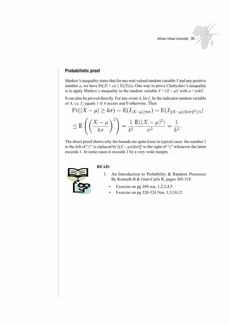
African Virtual University �0
Probabilistic proof
Markov’s inequality states that for any real-valued random variable Y and any positive number a, we have Pr(|Y| > a) ≤ E(|Y|)/a. One way to prove Chebyshev’s inequality is to apply Markov’s inequality to the random variable Y = (X − μ)2 with a = (σk)2.
It can also be proved directly. For any event A, let IA be the indicator random variable
of A, i.e. IA equals 1 if A occurs and 0 otherwise. Then
The direct proof shows why the bounds are quite loose in typical cases: the number 1 to the left of “≥” is replaced by [(X − μ)/(kσ)]2 to the right of “≥” whenever the latter exceeds 1. In some cases it exceeds 1 by a very wide margin.
READ:
1. An Introduction to Probability & Random Processes By Kenneth B & Gian-Carlo R, pages 305-318
• Exercise on pg 309 nos. 1,2,3,4,5• Exercise on pg 320-324 Nos. 1,3,10,12

African Virtual University ��
Correlation Types
Correlation is a measure of association between two variables. The variables are not designated as dependent or independent. The two most popular correlation coeffi-cients are: Spearman’s correlation coefficient rho and Pearson’s product-moment correlation coefficient.
When calculating a correlation coefficient for ordinal data, select Spearman’s tech-nique. For interval or ratio-type data, use Pearson’s technique.
The value of a correlation coefficient can vary from minus one to plus one. A minus one indicates a perfect negative correlation, while a plus one indicates a perfect po-sitive correlation. A correlation of zero means there is no relationship between the two variables. When there is a negative correlation between two variables, as the value of one variable increases, the value of the other variable decreases, and vise versa. In other words, for a negative correlation, the variables work opposite each other. When there is a positive correlation between two variables, as the value of one variable increases, the value of the other variable also increases. The variables move together.
The standard error of a correlation coefficient is used to determine the confidence intervals around a true correlation of zero. If your correlation coefficient falls outside of this range, then it is significantly different than zero. The standard error can be calculated for interval or ratio-type data (i.e., only for Pearson’s product-moment correlation).
The significance (probability) of the correlation coefficient is determined from the t-statistic. The probability of the t-statistic indicates whether the observed correlation coefficient occurred by chance if the true correlation is zero. In other words, it asks if the correlation is significantly different than zero. When the t-statistic is calcula-ted for Spearman’s rank-difference correlation coefficient, there must be at least 30 cases before the t-distribution can be used to determine the probability. If there are fewer than 30 cases, you must refer to a special table to find the probability of the correlation coefficient.

African Virtual University ��
Example
A company wanted to know if there is a significant relationship between the total num-ber of salespeople and the total number of sales. They collect data for five months.
Variable 1 Variable 2207 6907180 5991220 6810205 6553190 6190
Correlation coefficient = .921 Standard error of the coefficient = ..068 t-test for the significance of the coefficient = 4.100 Degrees of freedom = 3 Two-tailed probability = .0263
Another Example
Respondents to a survey were asked to judge the quality of a product on a four-point Likert scale (excellent, good, fair, poor). They were also asked to judge the reputation of the company that made the product on a three-point scale (good, fair, poor). Is there a significant relationship between respondents perceptions of the company and their perceptions of quality of the product?
Since both variables are ordinal, Spearman’s method is chosen. The first variable is the rating for the quality the product. Responses are coded as 4=excellent, 3=good, 2=fair, and 1=poor. The second variable is the perceived reputation of the company and is coded 3=good, 2=fair, and 1=poor.
Variable 1 Variable 24 32 21 23 34 31 12 1
Correlation coefficient rho = .830 t-test for the significance of the coefficient = 3.332 Number of data pairs = 7
Probability must be determined from a table because of the small sample size.

African Virtual University ��
Regression
Simple regression is used to examine the relationship between one dependent and one independent variable. After performing an analysis, the regression statistics can be used to predict the dependent variable when the independent variable is known. Regression goes beyond correlation by adding prediction capabilities.
People use regression on an intuitive level every day. In business, a well-dressed man is thought to be financially successful. A mother knows that more sugar in her children’s diet results in higher energy levels. The ease of waking up in the morning often depends on how late you went to bed the night before. Quantitative regression adds precision by developing a mathematical formula that can be used for predictive purposes.
For example, a medical researcher might want to use body weight (independent variable) to predict the most appropriate dose for a new drug (dependent variable). The purpose of running the regression is to find a formula that fits the relationship between the two variables. Then you can use that formula to predict values for the dependent variable when only the independent variable is known. A doctor could prescribe the proper dose based on a person’s body weight.
The regression line (known as the least squares line) is a plot of the expected value of the dependent variable for all values of the independent variable. Technically, it is the line that “minimizes the squared residuals”. The regression line is the one that best fits the data on a scatterplot.
Using the regression equation, the dependent variable may be predicted from the inde-pendent variable. The slope of the regression line (b) is defined as the rise divided by the run. The y intercept (a) is the point on the y axis where the regression line would intercept the y axis. The slope and y intercept are incorporated into the regression equation. The intercept is usually called the constant, and the slope is referred to as the coefficient. Since the regression model is usually not a perfect predictor, there is also an error term in the equation.
In the regression equation, y is always the dependent variable and x is always the independent variable. Here are three equivalent ways to mathematically describe a linear regression model.
y = intercept + (slope x) + error
y = constant + (coefficient x) + error
y = a + bx + e
The significance of the slope of the regression line is determined from the t-statistic. It is the probability that the observed correlation coefficient occurred by chance if the true correlation is zero. Some researchers prefer to report the F-ratio instead of the t-statistic. The F-ratio is equal to the t-statistic squared.

African Virtual University ��
The t-statistic for the significance of the slope is essentially a test to determine if the regression model (equation) is usable. If the slope is significantly different than zero, then we can use the regression model to predict the dependent variable for any value of the independent variable.
On the other hand, take an example where the slope is zero. It has no prediction ability because for every value of the independent variable, the prediction for the dependent variable would be the same. Knowing the value of the independent variable would not improve our ability to predict the dependent variable. Thus, if the slope is not significantly different than zero, don’t use the model to make predictions.
The coefficient of determination (r-squared) is the square of the correlation coeffi-cient. Its value may vary from zero to one. It has the advantage over the correlation coefficient in that it may be interpreted directly as the proportion of variance in the dependent variable that can be accounted for by the regression equation. For example, an r-squared value of .49 means that 49% of the variance in the dependent variable can be explained by the regression equation. The other 51% is unexplained.
The standard error of the estimate for regression measures the amount of variability in the points around the regression line. It is the standard deviation of the data points as they are distributed around the regression line. The standard error of the estimate can be used to develop confidence intervals around a prediction.
Example
A company wants to know if there is a significant relationship between its advertising expenditures and its sales volume. The independent variable is advertising budget and the dependent variable is sales volume. A lag time of one month will be used because sales are expected to lag behind actual advertising expenditures. Data was collected for a six month period. All figures are in thousands of dollars. Is there a significant relationship between advertising budget and sales volume?
Independent Variable
Dependent Variable
4.2 27.16.1 30.43.9 25.05.7 29.77.3 40.15.9 28.8
Model: y = 10.079 + (3.700 x) + error Standard error of the estimate = 2.568 t-test for the significance of the slope = 4.095 Degrees of freedom = 4 Two-tailed probability = .0149 r-squared = .807

African Virtual University ��
You might make a statement in a report like this: A simple linear regression was performed on six months of data to determine if there was a significant relationship between advertising expenditures and sales volume. The t-statistic for the slope was significant at the .05 critical alpha level, t(4)=4.10, p=.015. Thus, we reject the null hypothesis and conclude that there was a positive significant relationship between advertising expenditures and sales volume. Furthermore, 80.7% of the variability in sales volume could be explained
READ:
1) An Introduction to Probability & Random Processes By Kenneth B & Gian-Carlo R, pages 18-30, 212-215, 300-303
2) Robert B. Ash, Lectures on Statistics, page 28-29.
Ref: http://en.wikipedia.org/wiki/Correlation
Ref: http://en.wikipedia.org/wiki/Regression

African Virtual University ��
Chi-square Test
A chi-square test is any statistical hypothesis test in which the test statistic has a chi-square distribution when the null hypothesis is true, or any in which the probability distribution of the test statistic (assuming the null hypothesis is true) can be made to approximate a chi-square distribution as closely as desired by making the sample size large enough.
Specifically, a chi-square test for independence evaluates statistically significant differences between proportions for two or more groups in a data set.
• Pearson's chi-square test, also known as the Chi-square goodness-of-fit test • Yatεσ'chi−σquarεtεσt also known as Yates' correction for continuity • Mantel-Haenszel chi-square test • Linear-by-linear association chi-square test
In probability theory and statistics, the chi-square distribution (also chi-squared or c2 distribution) is one of the most widely used theoretical probability distributions in inferential statistics, i.e. in statistical significance tests. It is useful because, under reasonable assumptions, easily calculated quantities can be proven to have distribu-tions that approximate to the chi-square distribution if the null hypothesis is true.
If Xi are k independent, normally distributed random variables with mean 0 and va-
riance 1, then the random variable
is distributed according to the chi-square distribution. This is usually written
The chi-square distribution has one parameter: k - a positive integer that specifies the number of degrees of freedom (i.e. the number of X
i)
The chi-square distribution is a special case of the gamma distribution.
The best-known situations in which the chi-square distribution is used are the common chi-square tests for goodness of fit of an observed distribution to a theoretical one, and of the independence of two criteria of classification of qualitative data. However, many other statistical tests lead to a use of this distribution.

African Virtual University ��
Characteristic Function
The characteristic function of the Chi-square distribution is
Properties
The chi-square distribution has numerous applications in inferential statistics, for instance in chi-square tests and in estimating variances. It enters the problem of esti-mating the mean of a normally distributed population and the problem of estimating the slope of a regression line via its role in Student’s t-distribution. It enters all analysis of variance problems via its role in the F-distribution, which is the distribution of the ratio of two independent chi-squared random variables divided by their respective degrees of freedom.
Various chi and chi-square distributionsName Statistic
chi-square distribution
noncentral chi-square distribution
chi distribution
noncentral chi distribution
READ:
Ref: http://en.wikipedia.org/wiki/pearson%chi-square_testRef: http://en.wikipedia.org/wiki/Chi-Square_test

African Virtual University ��
Student’s T-test
A t test is any statistical hypothesis test for two groups in which the test statistic has a Student’s t distribution if the null hypothesis is true.
History
The t statistic was introduced by William Sealy Gosset for cheaply monitoring the quality of beer brews. “Student” was his pen name. Gosset was a statistician for the Guinness brewery in Dublin, Ireland, and was hired due to Claude Guinness’s inno-vative policy of recruiting the best graduates from Oxford and Cambridge to apply biochemistry and statistics to Guinness’ industrial processes. Gosset published the t test in Biometrika in 1908, but was forced to use a pen name by his employer who regarded the fact that they were using statistics as a trade secret. In fact, Gosset’s identity was unknown not only to fellow statisticians but to his employer—the company insisted on the pseudonym so that it could turn a blind eye to the breach of its rules.
Today, it is more generally applied to the confidence that can be placed in judgments made from small samples.
Use
Among the most frequently used t tests are:
• A test of the null hypothesis that the means of two normally distributed popu-lations are equal. Given two data sets, each characterized by its mean, standard deviation and number of data points, we can use some kind of t test to determine whether the means are distinct, provided that the underlying distributions can be assumed to be normal. All such tests are usually called Student’s t tests, though strictly speaking that name should only be used if the variances of the two populations are also assumed to be equal; the form of the test used when this assumption is dropped is sometimes called Welch’s t test. There are different versions of the t test depending on whether the two samples are
o independent of each other (e.g., individuals randomly assigned into two groups), or
o paired, so that each member of one sample has a unique relationship with a particular member of the other sample (e.g., the same people measured before and after an intervention, or IQ test scores of a husband and wife).
If the t value that is calculated is above the threshold chosen for statistical significance (usually the 0.05 level), then the null hypothesis that the two groups do not differ is rejected in favor of an alternative hypothesis, which typically states that the groups do differ.
• A test of whether the mean of a normally distributed population has a value specified in a null hypothesis.
• A test of whether the slope of a regression line differs significantly from 0.
Once a t value is determined, a P value can be found using a table of values from Student’s t-distribution.

African Virtual University ��
Confidence intervals using a small sample size
Consider a normally distributed population. To estimate the population’s variance take a sample of size n and calculate the sample’s variance, s. An unbiased estimator of the population’s variance is
Clearly for small values of n this estimation is inaccurate. Hence for samples of small size instead of calculating the z value for the number of standard deviations from the mean
and using probabilities based on the normal distribution, calculate the t value
The probability that the t value is within a particular interval may be found using the t distribution. The sample’s degrees of freedom are the number of data that need to be known before the rest of the data can be calculated.
e.g.
A random sample of things have weights
30.02, 29.99, 30.11, 29.97, 30.01, 29.99
Calculate a 95% confidence interval for the population’s mean weight.
Assume the population ~ N(μ,σ2)
The samples’ mean weight is 30.015 with standard deviation of 0.045. With the mean and the first five weights it is possible to calculate the sixth weight. Consequently there are five degrees of freedom.
The t distribution tells us that, for five degrees of freedom, the probability that t > 2.571 is 0.025. Also, the probability that t < −2.571 is 0.025. Using the formula for t with t = ± 2.571 a 95% confidence interval for the populations mean may be found by making μ the subject of the equation.
i.e.
(29.97 < μ < 30.06)

African Virtual University �00
READ:
1. Introduction to Probability By Charles M. Grinstead, pages 18-30, 212-215, 300-303
2. Robert B. Ash, Lectures on Statistics, page 23-29.• Answer problems 1- 6 on pg 23.
Ref: http://en.wikipedia.org/wiki/Statistical_Hypothesis_testingRef: http://en.wikipedia.org/wiki/Null_hypothesis

African Virtual University �0�
qReflection
The study of Correlation, Regression Hypothesis testing and other Mathematical modelling maybe simplified through ICT. The following link enables trainees to learn modelling with ease
http://www.ncaction.org.uk/subjects/maths/ict-lrn.htm

African Virtual University �0�
Unit 3 Probability Theory ( 40 Hours)
Indicator Function
In mathematics, an indicator function or a characteristic function is a function defined on a set X that indicates membership of an element in a subset A of X.
The indicator function of a subset A of a set X is a function
defined as
The indicator function of A is sometimes denoted
cA(x) or or even A(x).
Bonferoni Inequality
Let be the probability that is true, and be the probability that at least one of , , ..., is true. Then “the” Bonferroni inequality, also known as Boole’s inequality, states that
where denotes the union. If and are disjoint sets for all and , then the inequa-lity becomes an equality. A beautiful theorem that expresses the exact relationship between the probability of unions and probabilities of individual events is known as the inclusion-exclusion principle.
A slightly wider class of inequalities are also known as “Bonferroni inequalities.”

African Virtual University �0�
Generating Function
In mathematics a generating function is a formal power series whose coefficients encode information about a sequence a
n that is indexed by the natural numbers.
There are various types of generating functions, including ordinary generating functions, exponential generating functions, Lambert series, Bell series, and Dirichlet series; definitions and examples are given below. Every sequence has a generating function of each type. The particular generating function that is most useful in a given context will depend upon the nature of the sequence and the details of the problem being addressed.
Generating functions are often expressed in closed form as functions of a formal argument x. Sometimes a generating function is evaluated at a specific value of x. However, it must be remembered that generating functions are formal power series, and they will not necessarily converge for all values of x.
If an is the probability mass function of a discrete random variable, then its ordinary
generating function is called a probability-generating function.
The ordinary generating function can be generalised to sequences with multiple indexes. For example, the ordinary generating function of a sequence a
m,n (where n
and m are natural numbers) is
Characteristic Function (Probability Theory)
In probability theory, the characteristic function of any random variable completely defines its probability distribution. On the real line it is given by the following formula, where X is any random variable with the distribution in question:
where t is a real number, i is the imaginary unit, and E denotes the expected value.
If FX is the cumulative distribution function, then the characteristic function is given
by the Riemann-Stieltjes integral

African Virtual University �0�
In cases in which there is a probability density function, fX, this becomes
If X is a vector-valued random variable, one takes the argument t to be a vector and tX to be a dot product.
Every probability distribution on R or on Rn has a characteristic function, because one is integrating a bounded function over a space whose measure is finite.
The continuity theorem
If the sequence of characteristic functions of distributions Fn converges to the cha-
racteristic function of a distribution F, then Fn(x) converges to F(x) at every value of
x at which F is continuous.
Uses Of Characteristic Functions
Characteristic functions are particularly useful for dealing with functions of inde-pendent random variables. For example, if X
1, X
2, ..., X
n is a sequence of independent
(and not necessarily identically distributed) random variables, and
where the ai are constants, then the characteristic function for S
n is given by
In particular, . To see this, write out the definition of characteristic function:
Observe that the independence of X and Y is required to establish the equality of the third and fourth expressions.
Because of the continuity theorem, characteristic functions are used in the most frequently seen proof of the central limit theorem.
Characteristic functions can also be used to find moments of random variable. Provided that nth moment exists, characteristic function can be differentiated n times and

African Virtual University �0�
READ:
1. Robert B. Ash, Lectures on Statistics, page 32 of 45:
Ref : http://en.wikipedia.org/wiki/Characteristic_function_%28probability_theory%29
Statistical Independence
In probability theory, to say that two events are independent intuitively means that the occurrence of one event makes it neither more nor less probable that the other occurs. For example:
• The event of getting a "6" the first time a die is rolled and the event of getting a "6" the second time are independent.
• By contrast, the event of getting a "6" the first time a die is rolled and the event that the sum of the numbers seen on the first and second trials is "8" are depen-dent.
• If two cards are drawn with replacement from a deck of cards, the event of drawing a red card on the first trial and that of drawing a red card on the second trial are independent.
• By contrast, if two cards are drawn without replacement from a deck of cards, the event of drawing a red card on the first trial and that of drawing a red card on the second trial are dependent.
Similarly, two random variables are independent if the conditional probability dis-tribution of either given the observed value of the other is the same as if the other’s value had not been observed.
Independent Events
The standard definition says:
Two events A and B are independent if and only if Pr(A ∩ B) = Pr(A)Pr(B).
Here A ∩ B is the intersection of A and B, that is, it is the event that both events A and B occur.
More generally, any collection of events -- possibly more than just two of them -- are mutually independent if and only if for any finite subset A
1, ..., A
n of the collection
we have

African Virtual University �0�
This is called the multiplication rule for independent events.
If two events A and B are independent, then the conditional probability of A given B is the same as the “unconditional” (or “marginal”) probability of A, that is,
There are at least two reasons why this statement is not taken to be the definition of independence: (1) the two events A and B do not play symmetrical roles in this statement, and (2) problems arise with this statement when events of probability 0 are involved.
When one recalls that the conditional probability Pr(A | B) is given by
(so long as Pr(B) ≠ 0 )
one sees that the statement above is equivalent to
which is the standard definition given above.
Random Sample
A sample is a subset chosen from a population for investigation. A random sample is one chosen by a method involving an unpredictable component. Random sampling can also refer to taking a number of independent observations from the same probability distribution, without involving any real population. A probability sample is one in which each item has a known probability of being in the sample.
The sample will usually not be completely representative of the population from which it was drawn— this random variation in the results is known as sampling error. In the case of random samples, mathematical theory is available to assess the sampling error. Thus, estimates obtained from random samples can be accompanied by measures of the uncertainty associated with the estimate. This can take the form of a standard error, or if the sample is large enough for the central limit theorem to take effect, confience intervals may be calculated.

African Virtual University �0�
Types of random sample
• A simple random sample is selected so that every possible sample has an equal chance of being selected.
• A self-weighting sample, also known as an epsem sample, is one in which every individual, or object, in the population of interest has an equal opportunity of being selected for the sample. Simple random samples are self-weighting.
• Stratified sampling involves selecting independent samples from a number of subpopulations (or strata) within the population. Great gains in efficiency are sometimes possible from judicious stratification.
• Cluster sampling involves selecting the sample units in groups. For example, a sample of telephone calls may be collected by first taking a collection of telephone lines and collecting all the calls on the sampled lines. The analysis of cluster samples must take into account the intra-cluster correlation which reflects the fact that units in the same cluster are likely to be more similar than two units picked at random.
Multinomial Distribution
In probability theory, the multinomial distribution is a generalization of the bino-mial distribution.
The binomial distribution is the probability distribution of the number of “successes” in n independent Bernoulli trials, with the same probability of “success” on each trial. In a multinomial distribution, each trial results in exactly one of some fixed finite number k of possible outcomes, with probabilities p
1, ..., p
k (so that p
i ≥ 0 for
i = 1, ..., k and ), and
there are n independent trials. Then let the random variables Xi indicate the number
of times outcome number i was observed over the n trials. follows a multinomial distribution with parameters n and p.
Solutions from Multinomial Distribution Formula
A short version of the multinomial formula for three consecutive outcomes is given below.
If X consists of events E1, E2, E
3, which have the corresponding probabilities
of p1,
p2,
and p
3 of occurring, where x
1 is the number of times E
1 will occur,
x2 is the number of times E
2 will occur, and x
3 is the number of times E
3 will
occur, then the probability of X is

African Virtual University �0�
n!x1 ! x2 ! x3 !
.1
x1p .2
x2p .3
x3p where x1 + x
2 + x
3 = n and p
1 + p
2 + p
3 = 1
Example
1) In a large city, 60% of the workers drive to work, 30% take the bus, and 10% take the train. If 5 workers are selected at random, find the probability that 2 will drive, 2 will take the us, and 1 will take the train.
Solution
n= 5, x1=2, x
2 = 2, x
3= 1 and p
1=0.6, p
2= 0.3, and p
3 = 0.1
Hence, the probability that 2 workers will take the bus, and one will take the train is
5 !2 ! 2 !1!
. (20.6) 2(0.3) 1(0.1) = 0.0972
2) A box contains 5 red balls, 3 blue balls, and 2 white balls. If 4 balls are selected with replacement, find the probability of getting 2 red balls, one blue ball, and one white ball.
Solution
n=4, x1=2, x
2=1, x
3=1, and p
1=
510
, p2=
310
, and p3=
210
.
Hence, the probability of getting 2 red balls, one blue ball, and one white ball is
4!2!1!1!
510
⎛⎝⎜
⎞⎠⎟
2 310
⎛⎝⎜
⎞⎠⎟
1 210
⎛⎝⎜
⎞⎠⎟
1
= 12 3200
⎛⎝⎜
⎞⎠⎟=
950
= 0.18
{ Allan G, 2005, pg 132}

African Virtual University �0�
Order Statistic
Probability distributions for the n = 5 order statistics of an exponential distribution with q = 3.
In statistics, the kth order statistic of a statistical sample is equal its kth-smallest value. Together with rank statistics, order statistics are among the most fundamental tools in non-parametric statistics and inference.
Important special cases of the order statistics are the minimum and maximum value of a sample, and (with some qualifications discussed below) the sample median and other sample quartiles.
When using probability theory to analyse order statistics of random samples from a continuous distribution, the cumulative distribution function is used to reduce the analysis to the case of order statistics of the uniform distribution.
READ:
1. Robert B. Ash, Lectures on Statistics, page 25 -26 and Answer problems 1-4 on pg 26/27.
Ref: http://en.wikipedia.org/wiki/probability _distributionRef: http://en.wikipedia.org/wiki/RankingRef: http://en.wikipedia.org/wiki/non-parametric_Statistics
Notation and examples
For example, suppose that four numbers are observed or recorded, resulting in a sample of size n = 4. If the sample values are
6, 9, 3, 8,
they will usually be denoted
where the subscript i in xi indicates simply the order in which the observations were
recorded and is usually assumed not to be significant. A case when the order is si-gnificant is when the observations are part of a time series.
The order statistics would be denoted
where the subscript (i) enclosed in parentheses indicates the ith order statistic of the sample.

African Virtual University ��0
The first order statistic (or smallest order statistic) is always the minimum of the sample, that is,
where, following a common convention, we use upper-case letters to refer to random variables, and lower-case letters (as above) to refer to their actual observed values.
Similarly, for a sample of size n, the nth order statistic (or largest order statistic) is the maximum, that is,
The sample range is the difference between the maximum and minimum. It is clearly a function of the order statistics:
A similar important statistic in exploratory data analysis that is simply related to the order statistics is the sample interquartile range.
The sample median may or may not be an order statistic, since there is a single mid-dle value only when the number n of observations is odd. More precisely, if n = 2m + 1 for some m, then the sample median is X
(m + 1) and so is an order statistic. On the
other hand, when n is even, n = 2m and there are two middle values, X(m)
and X(m + 1)
, and the sample median is some function of the two (usually the average) and hence not an order statistic. Similar remarks apply to all sample quantiles.
Multivariate Normal Distribution
In probability theory and statistics, a multivariate normal distribution, also so-metimes called a multivariate Gaussian distribution, is a specific probability distribution, which can be thought of as a generalization to higher dimensions of the one-dimensional normal distribution (also called a Gaussian distribution).
Higher moments
The kth-order moments of X are defined by
where
The central k-order moments are given as follows
(a) If k is odd, .
(b) If k is even with k = 2λ, then

African Virtual University ���
where the sum is taken over all allocations of the set into λ (unorde-red) pairs, giving (2λ− 1)! / (2λ− 1(λ− 1)!) terms in the sum, each being the product of λ covariances. The covariances are determined by replacing the terms of the list
by the corresponding terms of the list consisting of r1 ones, then r
2
twos, etc, after each of the possible allocations of the former list into pairs.
In particular, the 4-order moments are
For fourth order moments (four variables) there are three terms. For sixth-order mo-ments there are 3 × 5 = 15 terms, and for eighth-order moments there are 3 × 5 × 7 = 105 terms.

African Virtual University ���
XV. synthesis of the Module
At the end of this module learners are expected to compute various measures of dis-persions and apply the laws of probability to various probability distributions. The learners should be able to solve various coefficients of correlation and regression. Unit one of Probability and Statistics covers Frequency distributions relative and cu-mulative distributions, various frequency curves, mean, Mode Median. Quartiles and Percentiles, Standard deviation, symmetrical and skewed distributions. The learner is introduced to various statistical measures and guided examples.
The examples are well illustrated and learners can follow without difficulty. It is recommended that learners attempt the formative evaluations given to assess their progress in the understanding of the content. Learners should take time to check the recommended reference material in CD’S, attached open source materials and the recommended websites. Most importantly, learners are encouraged to read the content widely and attempt the questions after each topic. Unit two of the module takes learners through Moment and moment generating function, Markov and Chebychev inequali-ties, special Univariate distributions, Bivariate probability distribution; Joint Marginal and conditional distributions; Independence; Bivariate expectation Regression and Correlation; Calculation of regression and correlation coefficient for bivariate data. Distribution function of random variables, Bivariate normal distribution. Derived distributions such as Chi-Square, t and F.
Unit two has various learning activities to aid learning and learners are advised to master the content of the various sub-topics and assess themselves through the formative evaluations. Failure to answer the formative assessments should be a positive indicator that learners should revise the sub-topics before progressing to other sub-topics. The tasks given under the different learning activities demands that you demonstrate a high level of ICT skills competency. The learning objectives are well stated in the beginning of the module and should guide learners in the level of expectations of the module.
Unit three focuses on probability theory and concentrates on the various probability distributions.
The summative evaluation will be used to judge the learners mastery of the module. It is recommended that learners revise the module before sitting for the final sum-mative evaluation.

African Virtual University ���
XVI. summative evaluation
Answer any four questions. Each question carries 15 marks.
Question 1: General Statistics
1) In the following table, the weights of 40 cows are recorded to the nearest kilo-gram.
128 161 135 142 145 156 150 145157 138 150 147 140 125 144 173144 146 140 176 154 148 163 164135 146 142 142 149 119 134 158165 168 138 147 152 153 136 126
Find;
a). the highest weightb). the least weightc). the ranged). construct a frequency distribution table starting with a class of 118-126e). calculate the mean of the dataf). calculate the standard deviation
Question 2: General Probability
2) A). A coin and a die are thrown together. Draw a possibility space diagram and find the probability of obtaining:
a). a headb). a number greater than 4c). a head and a number greater than 4d). a head or a number greater than 4
B). Events M and N are such that P(M) =1930
, P(N) =25
and P(M U N)=45
. Find
P(M I N).

African Virtual University ���
Question 3: Poisson Distribution
3) A book contains 500 pages and has 750 misprints.
a). What is the average number of misprints per page?
b) Find the probability that page 427 contains
i). no misprints
ii). exactly 4 misprints
c). find the probability that pages 427 and 428 will contain no misprints
Question 4: Continuous Random Variable
4) A continuous random variable (r.v) X has a probability density function (p.d.f) f(x) where
f (x) =
k(x + 2)2 − 2 ≤ x p 04k 0 ≤ x ≤ 1 1
3
0 otherwise
⎧
⎨
⎪⎪
⎩
⎪⎪
a) Find the value of the constant k
b) Sketch y=f(x)
c) Find P( - 1 ≤ X ≤ 1)
d) Find P(x>1)
Probability of an event
5). Given that P(AUB) =7/8, P(A I B)=1/4 and P(A’)=5/8, find the values of
a) P(A)
b) P(B)
c) P(A I B’)
d) P(A’U B’)
e) The probability that only one of A, B will occur.

African Virtual University ���
Expected Value
6). The continuous random variable r.v has the p.d.f
f (x) = x +
12
0 ≤ x ≤ 1
Find:
a).E(X)
b).E(24X +6)
c).E( 1-X)1
2
7). The masses, to the nearest kg, of 50 boys are recorded below.
Mass (kg) 60-64 65-69 70-74 75-79 80-84 85-89Frequency (f) 2 6 12 14 10 6
a).Construct a cumulative frequency curve
b).Use the curve to estimate the ;
i) Median
ii). Interquartile range
iii). 7th decile
iii). 60th percentile.

African Virtual University ���
Marking Scheme Of Summative Evaluation
1). a)176
b) 119
c) 176-119=57
d) Using 7 classes gives us a class interval of 9
Weight(kg) Tally Frequency118-126 /// 3
127-135 //// 5
136-144 //// //// 9
145-153 //// //// // 12
154-162 //// 5
163-171 //// 4
172-180 // 2
Total 40
e) Accept any method of calculating the mean
f). Accept any method of calculating the standard deviation
2) A). A coin has either Head(H) or Tail(T) while a die has sides 1,2,3,4,5&6.
Coin / Die 1 2 3 4 5 6Coin H H1 H2 H3 H4 H5 H6Coin T T1 T2 T3 T4 T5 T6
Sample space=12.
a). 6/12=1/2 b). 4/12=1/3c). 2/12=1/6d). 8/12=2/3

African Virtual University ���
B) . P(M U N)= P(M)+P(N)-P(M I N).
⇒45
= 1930
+ 25
- P(M I N).
⇒P(M I N) = 1930
+1230
−2430
=730
3). a) average number per page = 750/500=1.5
b) Let X be ‘the number of misprints per page’. Then, assuming that misprints
occur at random, X ~ P0(1.5)
i). P(X= 0) = e-1.5
= 0.2231…
P(there will be no misprints on page 427) = 0.223 ( 3d.p).
ii). P(X=4)= e-1.5 (1.5)4
4!= 0.0470…
P( there will be 4 misprints on page 427) = 0.047 ( 3d.p)
c). We expect 1.5 misprints on each page and so on two pages 427 & 428 we expect 1.5 + 1.5 = 3 misprints.
Let Y be the ‘’number of misprints on two pages’’
Y ~ P(3), so P0(Y=0)= e-3
= 0.4421
4). a). Since X is a random variable, then f (x)dxall x
∫ = 1
Therefore k(x + 2)2 dx + 4kdx0
113∫
−2
0∫ = 1
k3
(x + 2)3⎡⎣⎢
⎤⎦⎥−2
0+ 4k x[ ]0
113 = 1

African Virtual University ���
k3
(8) + 4k43
⎛⎝⎜
⎞⎠⎟
= 1 8k=1
k=18
a) The p.d.f of X is
- 2 0 3
11
x
y
21
y
c)
P(-1 ≤ x ≤ 0 ) =18
(x + 2)2
−1
0
∫ dx =7
24
and
P (0 ≤ x ≤ 1) = area of rec tan gle =12
Therefore
P (−1 ≤ X ≤ 1) = 724
+12=
1924

African Virtual University ���
d).
P(0≤ X ≤ 1) = area of rectangle=13×
12=
16
.
Therefore P(x>1) = 16
5) a) P(A)=1-P(A’)=1- 5/8=3/8
b) P(AUB)=P(A) – P(B) – P(A I B)
7/8=3/8+P(B) – ¼
P(B)=3/4
c) P(A I B’)=P(A) – P(A I B)
= 3/8-1/4
=1/8
d) A’ U B’ = (A I B)’ and P(A’U B’) = 1 – P(A I B) = 3/4
e) Only one of A, B occurs = (A I B’)U((A’ I B).
P(only one of A,Boccurs) = P(A I B’)+P(A’ I B)
= { P(A)-P(A I B)} + { P(B)-P(A I B)}
= 1/8 + ½ =5/8
6). a).E(X)=7/8
b).E(24X+6)=20
c).E( 1-X)1
2 = (1− x)1
2
0
1
∫ (x +12
)dx =35

African Virtual University ��0
7). a). Medium= 76.3 kg.
b). Interquartile range = 9 kg
c). Estimate of7
10× 50 = 35th decile from curve.
d). Estimate of 60
100× 50 = 30th percentile from curve

African Virtual University ���
XVII. References
http://en.wikipedia.org/wiki/Statistics
A concise Course in A-Level Statistics By J. Crawshaw and J.Chambers, Stanley Thornes Publishers, 1994
http://en.wikipedia.org/wiki/Probability
Business Calculation and Statistics Simplified, By N.A. Saleemi, 2000
http://microblog.routed.net/wp-content/uploads/2007/01/onlinebooks.html
Statistics: concepts and applications, By Harry Frank and Steven C Althoen, Cam-bridge University Press, 2004
http://mathworld.wolfram.com/Statistics
http://mathworld.wolfram.com/Probability
Probability Demystified, By Allan G. Bluman, McGraw Hill, 2005.
http://directory.fsf.org/math/
http://microblog.routed.net/wp-content/uploads/2007/01/onlinebooks.html
Lectures on Statistics, By Robert B. Ash, 2005.
Introduction to Probability, By Charles M. Grinstead and J. Laurie Snell, Swarthmore College.
http://directory.fsf.org/math/
Simple Statistics, By Frances Clegg, Cambridge University Press 1982.
Statistics for Advanced Level Mathematics, By I. Gwyn Evans University College of Wales, 1984.

African Virtual University ���
XVIII. student Records
Name of the EXCEL file
Mathematics: Probability and Statistics Student Records

African Virtual University ���
XIX. Main author of the Module
Mr. Paul Chege (B.Ed(Sc), M.Ed) [email protected]
The module author is a teacher trainer at Amoud University, Borama, Republic of Somaliland.
He has been a teacher trainer in Kenya, Republic of Seychelles, and Somalia. He has been involved in strengthening Mathematics and Sciences at secondary and tertiary levels under the Japan International Corporation Agency (JICA) programme in fifteen African countries.
He is married with three children.
XX. file structure Module Developer Writing Tip. The file naming and structure must follow the AVU/PI Consortium template as defined and explained by the AVU. Module Developers still need to provide the name of all the files (module and other files accompanying the module).
Daily, each module will be loaded in the personal eportfolio created for each consul-tant. For this, training will be provided by professor Thierry Karsenti and his team (Salomon Tchaméni Ngamo and Toby Harper).
Name of the module (WORD) file : Mathematics: Probability and Statistics ( Word)
Name of all other files (WORD, PDF, PPT, etc.) for the module.
1. Mathematics: Probability and Statistics Student Records ( Excel)2. Probability and Statistics: Marking Scheme for Summative Evaluation (
Word)3. An Introduction to Probability and Random Processes, Textbook by Kenneth
Baclawski and Gian-Carlo Rota ( 1979) ( PDF)4. Introduction To Probability, Textbook by Charles M. Grinstead and J. Laurie
Snell (PDF)5. Lectures on Statistics, Textbook by Robert B. Ash (PDF)