Embed Size (px)
Citation preview

U.S. DEPARTMENT OF THE INTERIOR
U.S. GEOLOGICAL SURVEY
Probability and Statisticsfor
Petroleum Resource Assessment
By
Robert A. Crovelli1
Open-File Report 93-582
This report is preliminary and has not been reviewed for conformity with U.S. Geological Survey editorial standards. Any use of trade, product or firm names is for descriptive purposes only and does not imply endorsement by the U.S. Government.
!U.S. Geological Survey, Box 25046, MS 971, DFC, Denver, Colorado 80225
1993

TABLE OF CONTENTS
PageVenn diagram for describing the fields of probability and statistics ................ 1The relationship between probability and inferential statistics......................... 2
I. Probability.................................................................................................................. 3A. Basic Concepts.................................................................................................... 4
1. Petroleum accumulation classification hierarchy................................... 42. Experiment, sample space, and event....................................................... 53. Venn diagram............................................................................................... 64. Tree diagram................................................................................................. 65. Event relations.............................................................................................. 76. Combinatorial analysis (counting techniques)........................................ 87. Definitions of probability............................................................................ 98. Probability of event relations..................................................................... 119. Conditional probability............................................................................... 12
10. Probability rules........................................................................................... 1311. Applications of probability rules............................................................... 1412. Bayes 1 rule..................................................................................................... 18
B. Random Variables and Probability Distributions......................................... 191. Discrete random variables.......................................................................... 192. Discrete probability distributions.............................................................. 203. Graphs of discrete probability distributions............................................ 214. Continuous random variables ................................................................... 225. Continuous probability distributions....................................................... 236. Graphs of continuous probability distributions...................................... 247. General graphs of continuous probability distributions........................ 258. Monte Carlo simulation.............................................................................. 26
C. Descriptive Parameters..................................................................................... 291. Measures of central location....................................................................... 29
a. Mean........................................................................................................ 29b. Median..................................................................................................... 30c. Mode........................................................................................................ 31
2. Mean, median, and mode related to skewness ....................................... 323. Measures of variation.................................................................................. 33
a. Variance................................................................................................... 33b. Standard deviation................................................................................ 34
4. Fractiles.......................................................................................................... 355. Examples....................................................................................................... 366. LOGRAF........................................................................................................ 39
D. Some Continuous Probability Distributions.................................................. 441. Normal distribution..................................................................................... 442. PROBDIST model selection menu............................................................. 453. 7-fractile probability histogram................................................................. 464. 3-fractile probability histogram................................................................. 47

5. Normal distribution (minimum/maxiinum)........................................... 486. Normal distribution (mean/standard deviation)................................... 497. Truncated normal distribution.................................................................. 508. Lognormal distribution............................................................................... 519. Truncated lognormal distribution............................................................. 52
10. Exponential distribution............................................................................. 5311. Truncated exponential distribution .......................................................... 5412. Pareto distribution....................................................................................... 5513. Truncated Pareto distribution.................................................................... 5614. Uniform distribution................................................................................... 5715. Triangular distribution ............................................................................... 58
H. Statistics .................................................................................................................. 59A. Sampling Concepts............................................................................................ 60
1. Populations................................................................................................... 602. Parameters.................................................................................................... 623. Samples.......................................................................................................... 644. Sampling techniques ................................................................................... 695. Statistics......................................................................................................... 71
B. Descriptive Statistics.......................................................................................... 731. Tabular methods.......................................................................................... 73
a. Frequency distribution.......................................................................... 73b. Relative frequency distribution........................................................... 74c. Cumulative frequency distribution (less than).................................. 75d. Relative cumulative frequency distribution (less than)................... 76e. Cumulative frequency distribution (more than)............................... 77f. Relative cumulative frequency distribution (more than)................. 78
2. Pictorial methods......................................................................................... 79a. Frequency histogram............................................................................. 79b. Relative frequency histogram.............................................................. 80c. Cumulative frequency polygon (less than)........................................ 81d. Relative cumulative frequency polygon (less than)......................... 82e. Cumulative frequency polygon (more than)..................................... 83f. Relative cumulative frequency polygon (more than)....................... 84
3. Measures of central location....................................................................... 85a. Sample mean .......................................................................................... 85b. Sample median....................................................................................... 86c. Sample mode.......................................................................................... 87
4. Measures of variation.................................................................................. 88a. Sample variance..................................................................................... 88b. Sample standard deviation................................................................... 89c. Sample range.......................................................................................... 90
C. Sampling Distributions..................................................................................... 911. Sampling distribution of the mean............................................................ 912. Central Limit Theorem................................................................................ 933. Normal probability paper........................................................................... 96
ii

D. Inferential Statistics ........................................................................................... 981. Statistical estimation.................................................................................... 100
a. Point estimation..................................................................................... 100b. Interval estimation................................................................................. 103
2. Tests of hypotheses...................................................................................... 104a. Z test for p................................................................................................ 104b. Chi-squared goodness-of-fit test.......................................................... 106c. Lognormal probability paper............................................................... 108
3. Regression and correlation......................................................................... Illa. formulas.................................................................................................. Illb. Transformations..................................................................................... 113c. Finding-rate curves................................................................................ 119d. Power laws.............................................................................................. 123e. Fractals..................................................................................................... 125
Selected References............................................................................................................ 130Appendix: Tables.............................................................................................................. 132A.I. Areas under the normal curve................................................................................ 132A.2. Critical values of the chi-squared distribution..................................................... 134Index..................................................................................................................................... 136
111

Ven
n D
iagr
am fo
r D
escr
ibin
g th
e F
ield
s of
Pro
babi
lity
and
Sta
tistic
s
Pro
babi
lity
Sta
tistic
s
AR
EA
S
Ope
ratio
ns R
esea
rch
Pro
babi
lity
Mod
els
Sto
chas
tic P
roce
sses
M
arko
v C
hain
s Q
ueui
ng T
heor
y S
imul
atio
n G
ame
The
ory
Dec
isio
n T
heor
y R
isk
Ana
lysi
s D
ynam
ic P
rogr
amm
ing
Rel
iabi
lity
The
ory
Com
bina
toria
l Ana
lysi
s T
ime
Ser
ies
Ana
lysi
s A
ctua
rial A
naly
sis
Ran
dom
Wal
ks
Pro
babi
lity
The
ory
Bas
ic
Pro
babi
lity
AR
EA
SS
tatis
tical
Inf
eren
ce
Est
imat
ion
The
ory
Tes
ts o
f Hyp
othe
ses
Reg
ress
ion
& C
orre
latio
n(S
impl
e &
Mul
tiple
) A
naly
sis
of V
aria
nce
Sta
tistic
al
Des
ign
of E
xper
imen
ts
The
ory
Sam
plin
g T
echn
ique
s S
ampl
e S
urve
ys
Non
para
met
ric S
tatis
tics
Mul
tivar
iate
Sta
tistic
s F
acto
r A
naly
sis
Dis
crim
inat
e A
naly
sis
Qua
lity
Con
trol
D
escr
iptiv
e S
tatis
tics
Bay
esia
n S
tatis
tics
Geo
stat
istic
s
The Relationship Between Probability and Inferential Statistics
Probability ^-"-"" ^^
(deductive reasoning)
Population Sample
(inductive reasoning)*"--- -* Statistics


I. Probability
A. Basic Concepts
1. Petroleum accumulation classification hierarchy
Pool: An individual accumulation or reservoir of oil or gas.
Field: A set of one or more pools of oil or gas that are related to a single
structural or stratigraphic feature.
Prospect: A potential oil or gas field.
Play: A set of one or more prospects that are geologically related in their
hydrocarbon sources, reservoirs, traps, and geologic histories.
Province (or basin): A set of one or more plays that are hydrodynamically
related.
Region: A set of one or more provinces that are geographically related.
O Prospect

2. Experiment, sample space, and event
Experiment: any process or action that generates observations.
Experiment: Three-prospect assessment
Suppose we are assessing three prospects in a new play. Each prospect
results in one of two possible outcomes. Let "success" (S) denote having an
oil or gas field and "failure" (F) denote being dry.
Sample space: a set of all possible outcomes (sample points) of an
experiment.Sample Space
SSS SSF SFS SFF FSS FSF FFS FFF
Event: a subset of a sample space.
Let event A: Exactly one field
A = {SFF, FSF, FFS}
and event B: At least one field
B = {SSS, SSF, SFS, SFF, FSS, FSF, FFS}

3. Venn diagram
Sample Space
FFF
4. Tree diagram
First Second Third Sample Event Prospect Prospect Prospect Point A
Event R
SSS
FFF

5. Event relations
a. Union of events
The union of two events A and B, denoted by AuB and read "A or B," is
the event containing all outcomes in A or B or both.
Let A = {SFF, FSF, FFS) and B = {SSS, SSF, SFS, SFF, FSS, FSF, FFS),
then AuB = {SSS, SSF, SFS, SFF, FSS, FSF, FFS}
b. Intersection of events
The intersection of two events A and B, denoted by AnB and read "A
and B," is the event containing all outcomes in both A and B.
Let A = {SFF, FSF, FFS} and B = {SSS, SSF, SFS, SFF, FSS, FSF, FFS},
then AnB = {SFF, FSF, FFS}
c. Complement of event
The complement of an event A, denoted by A' and read "not A," is the
event containing all outcomes of the sample space that are not in A.
Let A = {SFF, FSF, FFS},
then A' = {SSS, SSF, SFS, FSS, FFF}
d. Mutually exclusive events
Two events A and B are mutually exclusive or disjoint events
if A and B have no outcomes in common, i.ev AnB = 0
Let A = {SFF, FSF, FFS} and B = {SSF, SFS, FSS},
then AnB = 0
Therefore, A and B are mutually exclusive events.

6. Combinatorial analysis (counting techniques)
a. Fundamental principle of counting
If an operation can be performed in n, ways, and if for each of these a
second operation can be performed in n2 ways, and for each of the first
two a third operation can be performed in n3ways, and so forth, then
the sequence of k operations can be performed in n!n2 ...nk ways.
Experiment: Three-prospect assessment
Number of sample points in sample space = 2*2*2 = 8
b. Combinations
A combination is any unordered subset of r objects taken from a set of n
distinct objects.
The number of combinations of r objects taken from n distinct objects is
r!(n-r)!
where "n factorial" is n! = n(n-l)(n-2)» (3)(2)(1) and 0! = 1.
Number of sample points in event A = I , = = = 3 K v (I) 1121 1»2»1
(3\ (3} (3}_Number of sample points in event B = L + ~ + - -3 + 3 + 1-7
V 1 / Vz/ V-V
c. Permutations
A permutation is any ordered subset of r objects taken from a set of n
distinct objects.
The number of permutations of r objects taken from n distinct objects isp _ "I r'"~(^
The number of ways of selecting with order (permutations) 3 prospects
from a set of 5 prospects is5' 5'P3 5 =_^i = ± = 5-4-3 = 60
3p (5-3)! 2!
8
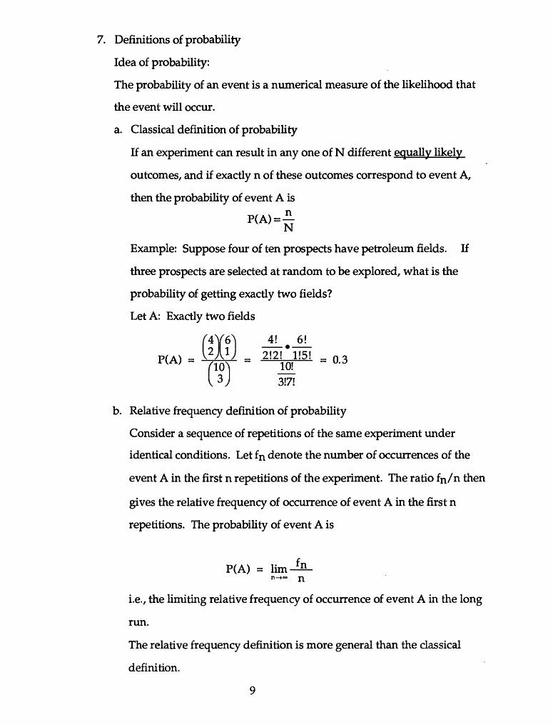
7. Definitions of probability
Idea of probability:
The probability of an event is a numerical measure of the likelihood that
the event will occur.
a. Classical definition of probability
If an experiment can result in any one of N different equally likely
outcomes, and if exactly n of these outcomes correspond to event A,
then the probability of event A is
Example: Suppose four of ten prospects have petroleum fields. If
three prospects are selected at random to be explored, what is the
probability of getting exactly two fields?
Let A: Exactly two fields
4X6 4! 6! P(A) - - 2!2! U ' ~ ' ~ 10!
317!
b. Relative frequency definition of probability
Consider a sequence of repetitions of the same experiment under
identical conditions. Let fn denote the number of occurrences of the
event A in the first n repetitions of the experiment. The ratio fn/n then
gives the relative frequency of occurrence of event A in the first n
repetitions. The probability of event A is
P(A) = lin->~ n
i.e., the limiting relative frequency of occurrence of event A in the long
run.
The relative frequency definition is more general than the classical
definition.
9

The relative frequency definition includes the classical definition.
Example: The probability of a dry hole in a particular explored basin is
0.8 from past statistical data,
c. Subjective definition of probability
A personal opinion (depending on the information held by a person at
some time) of the likelihood that an event will occur. Subjective
probability includes the case where past statistical data are not available
and/or the information available is of an indirect nature.
The subjective definition is more general than the relative frequency
definition.
The subjective definition includes the relative frequency definition.
In petroleum resource assessment the application, assignment and
interpretation of probability is based on the subjective definition of
probability.
Example: The probability of recoverable petroleum in an unexplored
play is 0.3 without past statistical data,
d. Axiomatic definition of probability
The probability of an event A is the sum of the weights of all sample
points in A. Therefore,
0 < P(A) < 1, P(0) = 0, and P(S) = 1
where 0 denotes the empty set and S the sample space.
The theory of probability is based on the axiomatic definition of
probability.
The classical and relative frequency definitions of probability can be
derived as theorems from the axiomatic definition.
10

8. Probability of event relations
Suppose we assume equally likely sample points for the experiment: three-
prospect assessment.Sample Space
SSS SSF SFS SFF FSS FSF FFS FFF
a. Given event A: Exactly one field
A = {SFF, FSF, FFS},
then P(A) = 3/8
b. Given event B: At least one field
B = {SSS, SSF, SFS, SFF, FSS, FSF, FFS},
then P(B) = 7/8
c Given AuB = {SSS, SSF, SFS, SFF, FSS, FSF, FFS},
then P(AuB) = 7/8
d. Given An B = {SFF, FSF, FFS},
then P(AnB) = 3/8
e. Given A1 = {SSS, SSF, SFS, FSS, FFF},
then P( A1 ) = 5/8
f. Given B1 = {FFF},
then P(B') = 1/8
11

9. Conditional probability
Notation P(A I B) denotes the conditional probability of event A given that
the event B has occurred.
Given that B has occurred, event B becomes the new reduced sample space.
Conditional probability:
For any two events A and B with P(B) > 0, the conditional probability of A
given that B has occurred is defined by
Consider the experiment: three-prospect assessment with equally likely
sample points.
P(B) 7/8
Independence:
Two events A and B are independent if P(A I B) = P(A) and are dependent
otherwise.
Consider the experiment: three-prospect assessment with equally likely
sample points. Since
P(A I B) = 3/7 and P(A) = 3/8 => P(A I B) * P(A),
events A and B are dependent.
Remark: If two events are mutually exclusive, then they are dependent.
12
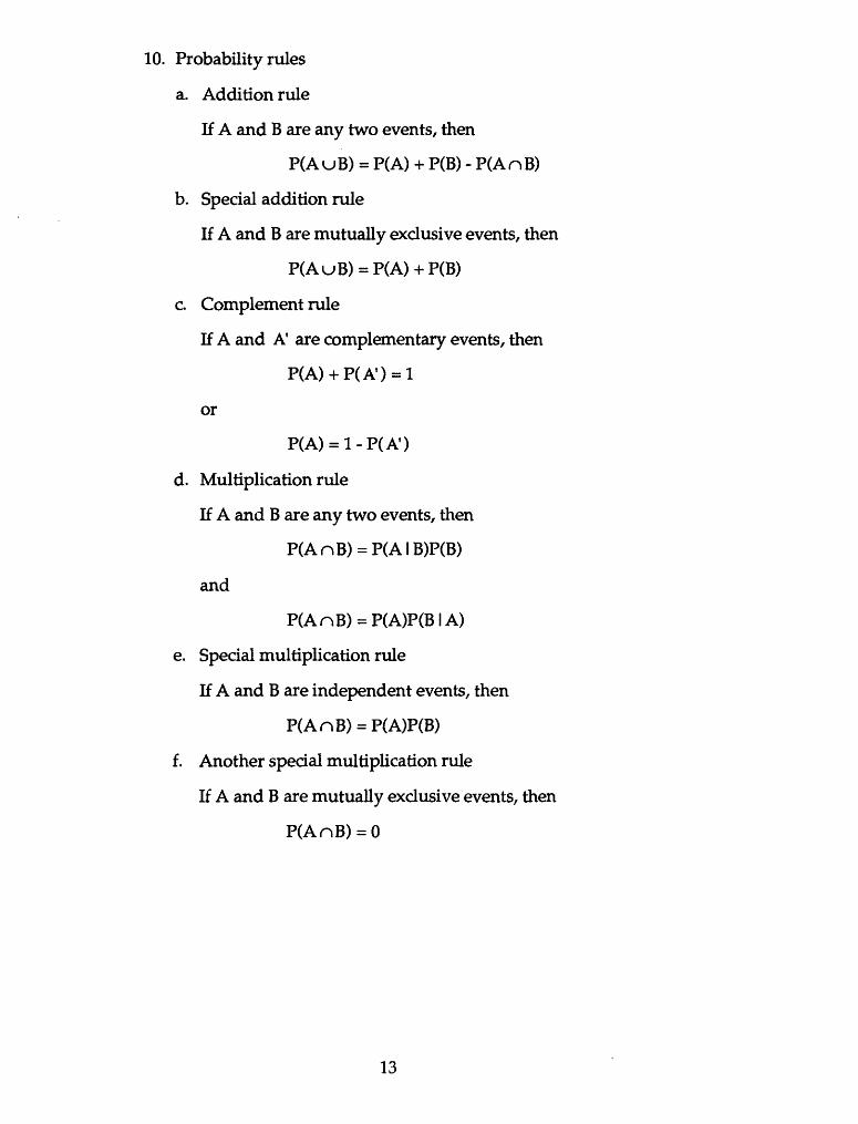
10. Probability rules
a. Addition rule
If A and B are any two events, then
P(AuB) = P(A) + P(B) - P(AnB)
b. Special addition rule
If A and B are mutually exdusive events, then
P(AuB) = P(A) + P(B)
c Complement rule
If A and A' are complementary events, then
P(A) + P(A') = 1
or
P(A) = 1-P(A')
d. Multiplication rule
If A and B are any two events, then
P(AnB) = P(AIB)P(B)
and
P(AnB) = P(A)P(BIA)
e. Special multiplication rule
If A and B are independent events, then
P(AnB) = P(A)P(B)
f. Another special multiplication rule
If A and B are mutually exdusive events, then
P(AnB) = 0
13

11. Applications of probability rules
a. Equally likely
First Second Third Sample Event Prospect Prospect Prnspprt Point A Probability
SSS 0.125
0.1250.125
0.1250.125
0.1250.125
0.1251.000
P(A) = P(SFF u FSF u FFS) = 3/8 = 0.375
or = P(SFF) + P(FSF) + P(FFS) = 0.125 + 0.125 + 0.125 = 0.375
or = P(S)P(F)P(F) + P(F)P(S)P(F) + P(F)P(F)P(S) = 3(0.5)3 = 0.375
14

b. Bernoulli process
First Second Third Sample Event Prospect Prospect Prospect Point A
SSS
SSF SFS
SFF FSS
FSF FFS
FFF
P(A) = P(SFF) + P(FSF) + P(FFS)
= P(S)P(F)P(F) + P(F)P(S)P(F) + P(F)P(F)P(S)
= 3P(S)P(F)P(F) = 3(0.2)(0.8)2 = 0.384
15

c. Independence
First Prospect
Second Third Sample Prospect Prospect Point
Event A
SSS
SSF SFS
SFF FSS
FSF FFS
FFF
P(A) = P(SiF2F3) + P(FiS2F3) + P(FiF2S3)
= P(Si)P(F2)P(F3) + P(Fi)P(S2)P(F3) + P(Fi)P(F2)P(S3)
= (0.2)(0.9)(0.7) + (0.8)(0.1)(0.7) + (0.8X0.9X0.3) = 0.398
16
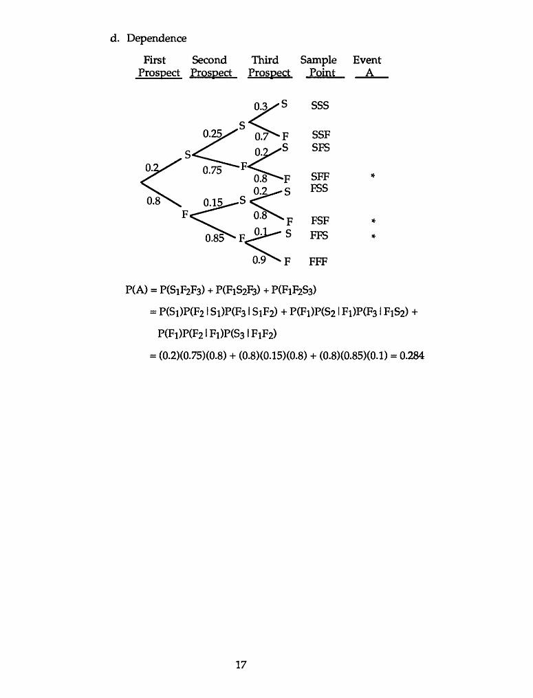
d. Dependence
First Second Third Sample Event Prospect Prospect Prospect Point A
SSS
0.8
FFF
P(A) = P(SiF2F3) + P(FiS2F3) + P(FiF2S3)
= P(Si)P(F2 1 Si)P(F3 1 SiF2) + P(Fi)P(S2 1 Fi)P(F3 1 FiS2) +
P(Fi)P(F2 lFi)P(S3 lFiF2)
= (0.2)(0.75)(0.8) + (0.8X0.15X0.8) + (0.8)(0.85)(0.1) = 0.284
17

12. Bayes'rule
Rule of total probability:
If the events BI, 62, ..., Bk constitute a partition of the sample space such
that P(Bi) * 0 for i = 1, 2, ..., k, then for any event Ak k
P(A) =
Example: Three-prospect assessment with two hypothesized possible
states of nature
BI: Exactly one field; estimated prior probability P(Bi) = 3/4
62: Exactly two fields; estimated prior probability P(B2) = 1/4
Let event A: First wildcat well drilled results in a dry hole
Conditional probabilities: P(A I BI) = 2/3 and P(A 1 62)= 1/3
Therefore, P(A) = P(Bi)P(A I BI) + P(B2)P(A I B2)
= (3/4X2/3) + (1/4)0/3) = 7/12
Bayes' rule:
If the events BI, 62, ..., Bk constitute a partition of the sample space, where
P(Bi) * 0 for i = 1, 2, ..., k, then for any event A such that P(A) * 0,
P(B |A)= P(BfnA) = P(Br )P(AIBr ) r P(A)
for r = 1, 2, ..., k.
Example: Posterior probabilities arePCBi I A) - P(Bi)P(AIBi)
P(B2 )P( Al B2 )
(3/4)(2/3)(3/4)(2/3) + (l/4)(l/3) 7/12
P(B2lA)= P(B2 )p(MB2) P(B1 )P(AIB1 ) + P(B2 )P(AIB2 )
(3/4)(2/3)+ (1/4X1/3) 7/12
18

B. Random Variables and Probability Distributions
A random variable X is a function that associates a real number with each
element in the sample space.
1. Discrete random variables
a. Binomial random variable
Bernoulli processFirst Second Third Sample
Prospect Prospect Prospect Point Probability x
SSS 0.008 3
SSF 0.032 2 SFS 0.032 2
SFF 0.128 1 FSS 0.032 2
FSF 0.128 1
FFS 0.128 1
FFF 0.512 0 1.000
Let random variable X: Number of fields (successes)
Possible distinct values x = 0,1,2,3
Note that P(X = 1) = P(A) = 0.384
A discrete random variable X can take on a countable number of values.
b. Examples of discrete random variablesX: Number of discoveriesX: Number of dry holesX: Number of prospectsX: Number of petroleum accumulationsX: Number of oil fieldsX: Number of gas fieldsX: Number of exploratory wells
19

2. Discrete probability distributions
Probability distributions can be expressed in the form of tables, graphs, and
formulas.
Binomial distribution
a. Probability mass function (pmf)
f(x) = P(X = x)
x0
1
2
3
f(x)
0.512
0.3840.0960.008
1-f(x)0.5- 11 I . 1 1 1
0123
b. Cumulative (less than) distribution function (cdf)
F(x)=P(X<x)
F(x) =
0 forx < 0 0.512 for 0 < x < 1 0.896 for 1 < x < 2 0.992 for 2 < x < 3 1 for x > 3
c. Complementary cumulative (more than) distribution function (ccdf)
R(x) = P(X > x) = 1 - F(x)
R(x) =
1 for x < 0 0.488 for 0 < x < 1 0.104 for 1 < x < 2 0.008 for 2 < x < 3 0 forx > 3
20

3. Graphs of discrete probability distributions
Binomial distribution
a. Probability histogram
U L
Are
I 1"T"I
Area represents probability
0123
b. Cumulative (less than) distribution function (cdf)
F(x)
0 2 3
c. Complementary cumulative (more than) distribution function (ccdf) R(x)r-
o-f r-2 3
21

4. Continuous random variables
a. Concept of a continuous random variable
A continuous random variable X can take on a continuum of values.
X = x where x is a real number in an interval, e.g., 0 < x «» or any
positive number.
p is area between x 1 and \2.
Total area under curve equals 1.
1 2
P(XI < X < X2> = p
b. Examples of continuous random variables
X: Oil field size
X: Gas field size
X: Area of closure
X: Reservoir thickness
X: Reservoir depth
X: Effective porosity
X: Hydrocarbon saturation
X: Reservoir pressure
X: Reservoir temperature
22

5. Continuous probability distributions
Uniform or rectangular distribution
a. Probability density function (pdf)
1
f(x) =b-a fora < x < b
otherwise
Parameters: a and b real numbers with a < b
b. Cumulative (less than) distribution function (cdf)
F(x)=P(X<x)
0 forx < a
F(x) = < for a < x < b
1 forx > b
c. Complementary cumulative (more than) distribution function (ccdf)
R(x) = P(X > x) = 1 - F(x)
1 for x < a R(x) = < for a < x < bb-a
0 for x > b
23

6. Graphs of continuous probability distributions
Uniform or rectangular distribution
a. Probability density function (pdf)
f(x)
b-a
0 a b
b. Cumulative (less than) distribution function (cdf)
F(x)
1
0 a b
c. Complementary cumulative (more than) distribution function (ccdf)
R(x)
1
24

7. General graphs of continuous probability distributions
a. Probability density function (pdf)
f(x)
b. Cumulative (less than) distribution function (cdf)
F(x)=P(X< x)
c. Complementary cumulative (more than) distribution function (ccdf)
R(x) = P(X>x) = l-F(x) R(x)
25

8. Monte Carlo simulation
a. Binomial distribution
X: Number of fields (successes) in 3 prospects (x = 0,1,2,3).
P(field) = 0.2 and P(dry) = 0.8
X = Xi + X2 + X3 where
Xi: Number of fields in prospect 1 (xi = 0,1),
X2: Number of fields in prospect 2 (x2 = 0,1),
Xy Number of fields in prospect 3 (xs = 0,1).
0 1 Prospect 1
U
0 1 X2 Prospect 2
0 1 Prospect 3
X3
Make 5000 simulation passes and compute X each pass.
On each pass, select 3 random numbers (Ui, U2, U3) between 0 and 1.
Ui is uniformly distributed over the interval [0,1].
If 0 < Ui < 0.8 assign 0, and if 0.8 < Ui < 1 assign 1.
Generate a relative frequency distribution from the 5000 values of X.
For example,Pass No.
123
.
5000
Ui0.560.710.89
.0.47
U20.820.630.95
.
.
.0.08
U30.120.290.38
.
.
0.69
Xi001..
0
X2101.
.
0
X3000
.
0
X102
.
0
26

A relative frequency distribution of X from an actual simulation,
compared to the exact probability distribution of X from the analytic
method:
f(x)X
0123
freq.2590190046644
rel. freq.0.5180.3800.0930.009
b. Probability distribution for field size
X: Oil field size (barrels),
X = Xi X2 Xa where
Xi: Area of closure (acres),
X2: Reservoir thickness (feet),
X3: Oil yield factor (barrels/acre-foot).
R2 (x 2)
U2 __J
ClosureX 2
Thickness
0.5120.3840.0960.008
R3 (x3)
U
X 3 ^ Oil Yield Factor
Make 5000 simulation passes and compute X each pass.
On each pass, select 3 random numbers (Ui, U2, Us) between 0 and 1.
Ui is uniformly distributed over the interval [0,1].
From Ui determine \ir from U2 determine X2, and from Us
determine XB, using their ccdf curves as inverse functions.
Generate a relative frequency distribution from the 5000 values of X
27
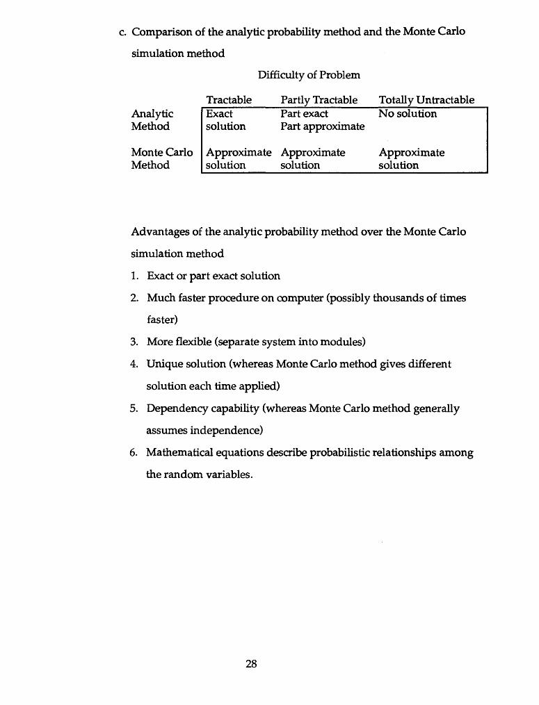
c. Comparison of the analytic probability method and the Monte Carlo
simulation method
Difficulty of Problem
Tractable Partly Tractable Totally UntractableAnalytic Method
Monte Carlo Method
Exact Part exact solution Part approximate
Approximate Approximate solution solution
No solution
Approximate solution
Advantages of the analytic probability method over the Monte Carlo
simulation method
1. Exact or part exact solution
2. Much faster procedure on computer (possibly thousands of times
faster)
3. More flexible (separate system into modules)
4. Unique solution (whereas Monte Carlo method gives different
solution each time applied)
5. Dependency capability (whereas Monte Carlo method generally
assumes independence)
6. Mathematical equations describe probabilistic relationships among
the random variables.
28

C. Descriptive Parameters
1. Measures of central location
Also called measures of central tendency
a. Mean
i. Probability density function (pdf)
mean center of gravity
ii. Experiment: Three-prospect assessment
Binomial random variable X: Number of fields
Binomial distribution: X
0 1 2 3
f(x)0.512 0.384 0.096 0.008
The mean or expected value of X is H= E(X) = Zxf(x)
X
= (0X0.512) + (1X0.384) + (2X0.096) + (3X0.008)
= 0.6
iii. Uniform or rectangular distribution
The mean or expected value of X is
H = E(X) = J_~ xf(x)dx
a + b
29

b. Median
i. Probability density function (pdf) f(x)
median
ii. Cumulative (less than) distribution function (cdf)F(x)
1
0.5 - - -
median
F (median) = P(X < median) = 0.5
iii. Complementary cumulative (more than) distribution function (ccdf)
R(x)
0
median
R(median) = P(X > median) = 0.5
30

c. Mode
i. Probability density function (pdf) f(x)
max
mode
ii. Cumulative (less than) distribution function (cdf)
Inflection point
mode
iii. Complementary cumulative (more than) distribution function
(ccdf)
Inflection point
mode
31

2. Mean, median, and mode related to skewness
a. Symmetric probability density function (pdf)
f(x)
meanmedianmode
b. Positively skewed probability density function (pdf)
f(x)
mode median
mean
c. Negatively skewed probability density function (pdf)
mean median
mode
32

3. Measures of variation
a. Variance
i. Two probability density functions with different variations
f(x)
B
Pdf A has more variation or dispersion or spread than pdf B.
ii. Experiment: Three-prospect assessment
Binomial random variable X: Number of fields
Binomial distribution: X
0123
t(x)0.5120.3840.0960.008
The mean of X is |i = 0.6
The variance of X is a2 ^ E[(X -
= (0 - 0.6)2 (0.512) + (1 - 0.6)2 (0.384) + (2 - 0.6)2 (0.096)
+(3 - 0.6)2(0.008)
= 0.48
Theorem: a2 = E(X2 )-^i2
E(X2) = (02)(0.512) + (l2)(0.384) + (22)(0.096) + (32)(0.008)
= 0.84
a2 = 0.84 -(0.6)2 = 0.48
33

b. Standard deviation
i. The standard deviation of X is the positive square root of the
variance of X, i.e.,
a =
ii. Experiment: Three-prospect assessment
Binomial random variable X: Number of fields
The standard deviation of X is
a = VO.48 = 0.69
iii. Chebyshev's Theorem:
Given any random variable X with mean |i and standard
deviation a, then
foranyk>0, P(u - ko< X < a + kcr) > 1 - -=-.\c
3 For k = 2, P(fj. - 20 < X < u + 2cr) > 4o
For k = 3, P(jU - 3cr < X < p, + 3cr) ^ -
iv. Experiment: Three-prospect assessment
Binomial random variable X: Number of fields
The mean of X is u = 0.6
The standard deviation of X is a = 0.69
For k = 2, P[0.6 - 2(0.69) < X < 0.6 + 2(0.69)]
= P(- 0.78 < X < 1.98) = 0.896 > 0.75
34

4. Fractiles
a. Fractiles are values of a random variable that correspond to "more than"
or excedence probabilities.
The pi00th fractile (0 < p < 1), denoted by Fpioo/ is the value of a random
variable X such that P(X > Fpioo) = P-
For example
The 95th fractile, Fgs, is the value of X such that P(X > Fgs) = 0.95.
The 5th fractile, FS, is the value of X such that P(X > FS) = 0.05.
The 50th fractile, FSQ, is the median,
b. Probability density function (pdf)
c. Complementary cumulative (more than) distribution function (ccdf)
R(x)
35

1.00
0.95
0.05
0.00
QUANTITY OF RECOVERABLE RESOURCE
QUANTITY OF RECOVERABLE RESOURCE
Figure 8. Typical conditional probability distribution of an undiscovered recoverable resource shown as A , conditional more-than cumulative distribution function, and B, conditional probability density function. FQC denotes the 95th fractile; the probability of more than the amount is 95 percent. Fr denotes the 5th fractile; the -probability of more than the amount is 5 percent.
Source: Dolton and others, 1981
36
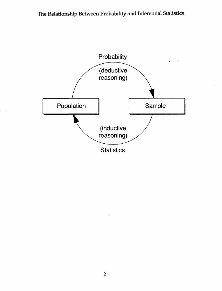
ESTIMRTESMERN - MEDIRN - 95X 757. 507. 257. 57.
MODE - 5.0.
1.08 0.73 0.18 0.40 0.73 1.32 3.H 0.33 1.19
4.8 6.0 7.2
BILLION BARRELS RECOVERABLE OIL
9.6 10.6 12.0
F5
6.0 7.2
BILLION BARRELS RECOVERABLE OIL
ESTIMRTESMERN -MEDIRN -95X757.50X25X57.
MODE -5.D.
1.080.730.180.400.731.323.140.331.19
9.6 10.8 12.0
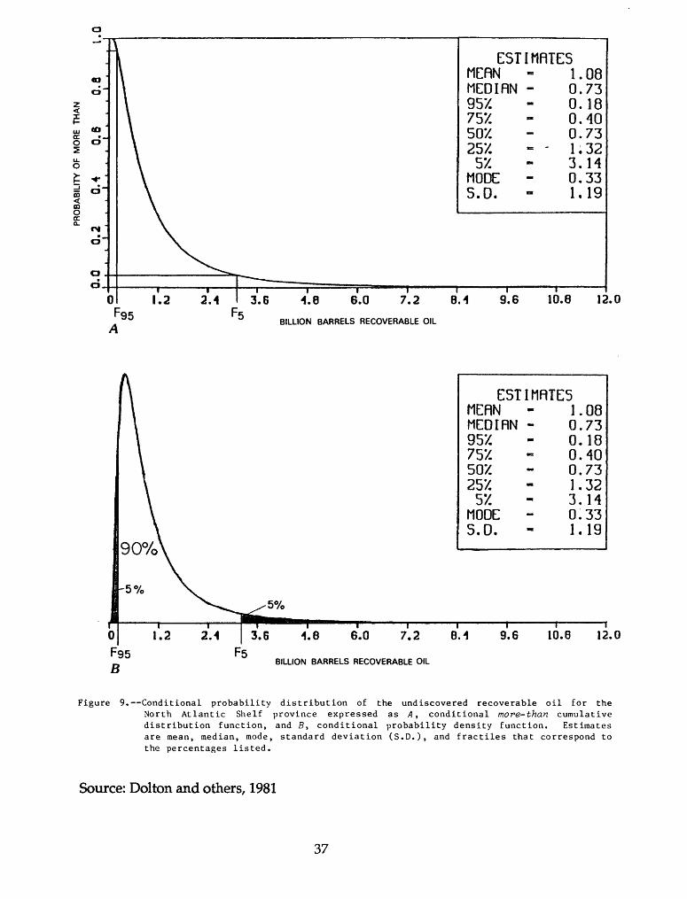
Figure 9. Conditional probability distribution of the undiscovered recoverable oil for the North Atlantic Shelf province expressed as A , conditional more-than cumulative distribution function, and B, conditional probability density function. Estimates are mean, median, mode, standard deviation (S.D.), and fractiles that correspond to the percentages listed.
Source: Dolton and others, 1981
37

oCM
o . z. cn <£ .^ Ri- .
o . LJor ^ '
O
5 , "cn oo "OQ 0_
£ §:
\
\
\\\V--_
ESTI MERN MEDIflN - 957. 757. 50X 257.
57. MODE - S.D.
MflTES 0.45 0.00 0.00 0.00 0.00 0.59 2.07 0.33 0.94
0.0 1.2 2.4 3.6 4.8 6.0 7.2BILLION BARRELS RECOVERABLE OIL
8.4 9.6 10.8 12.0
58%
E5TWRTESMERNMEDIRN - 957. 757. 507. 257.
5XMODE 5.0.
0.15 0.00 0.00 O.GO 0.00 0.59 2.07 0.33 0.94
6.0 7.2 8.1 9.6 10.8 I2.0
BILLION BARRELS RECOVERABLE OIL
Figure 10. Probability distribution of the undiscovered recoverable oil for the North Atlantic Shelf province expressed as A, more-than cumulative distribution function, and 5, probability density function. A has the value of the marginal probability (0.42) at zero resource. B has a spike at zero resource of probability weight 1-0.42=0.58 which represents the chance of no recoverable oil being present. Estimates are mean, median, mode, standard deviation (S.D.), and fractiles that correspond to percentages listed.
Source: Dolton and others, 1981
38

EXAMPLES
Examples of two probability curves on the same graph are (1) conditional and unconditional resource potential, and (2) recoverable and economically recoverable resource potential.
Example 1
LOGRAF is used to duplicate the probability graphs that were originally generated by EXACTDIS for the national assessment of undiscovered conventional oil and gas resources by the U.S. Geological Survey (Mast and others, 1989).
Figure la consists of cumulative probability distributions for undiscovered recoverable and undiscovered economically recoverable conventional crude oil resources of the United States. Figure la' is a summary of the input and output of the assessment, including the lognormal parameters and the conditional and unconditional estimates for each probability curve. The input into LOGRAF are estimates of the following parameters for each distribution:
Recoverable resources-p = 1, 6 = 0, F^5 = 33.2, F^ = 69.9
Economically recoverable-? = 1, 6 = 0, F^5 = 20.7, F£ = 53.8
and with units of billions of barrels.
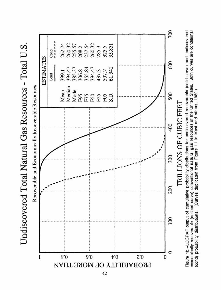
Figure Ib consists of cumulative probability distributions for undiscovered recoverable and undiscovered economically recoverable conventional natural gas resources of the United States. Figure lb' is a summary of the input and output of the assessment, including the lognormal parameters and the conditional and unconditional estimates for each probability curve. The input into LOGRAF are estimates of the following parameters for each distribution:
Recoverable resources-p = 1, 6 = 0, F^5 = 306.8, F^ = 507.2
Economically recoverable-p = 1, 0 = 0, F^5 = 208.2, F^ = 325.5
and with units of trillions of cubic feet.
39

Und
isco
vere
d C
onve
ntio
nal C
rude
Oil
Res
ourc
es -
Tot
al U
.S.
Rec
over
able
and
Eco
nom
ical
ly R
ecov
erab
le R
esou
rces
EST
IMA
TE
SC
ond
49.4
2348
.173
45.7
6933
.241
.354
48.1
7356
.117
69.9
11.3
29
020
Con
d
Mea
nM
edia
nM
ode
F95
F75
F50
F25
F05
S.D
.
34.8
0833
.372
30.6
7420
.727
.437
33.3
7240
.59
53.8
10.3
22
BIL
LIO
NS
OF
BA
RR
EL
SFi
gure
1a.
--LO
GR
AF
outp
ut o
f cu
mul
ativ
e pr
obab
ility
dis
tribu
tions
for
und
isco
vere
d re
cove
rabl
e (s
olid
cur
ve)
and
undi
scov
ered
ec
onom
ical
ly r
ecov
erab
le
(das
hed
curv
e) c
onve
ntio
nal
crud
e oi
l re
sour
ces
of t
he U
nite
d S
tate
s.
Both
cur
ves
are
cond
ition
al
(con
d) p
roba
bilit
y di
strib
utio
ns.
(Cur
ves
dupl
icat
ed f
rom
Fig
ure
10 i
n M
ast
and
othe
rs,
1989
.)

LOGRAF 92.7 15-Dec-1992 17:09:09 C:\LOGRAF\GEOTECH\USOIL.DAT
TitleSubtitleUnits
Undiscovered Conventional Crude Oil Resources - Total U.S. Recoverable and Economically Recoverable Resources BILLIONS OF BARRELS
INPUT: Probability curve # 1
Marginal probability Shift parameter Conditional F95 Conditional F05
OUTPUT:
Lognormal parameters Mu 3.8748 Sigma 0.2263
Conditional estimates Mean 49.423 Median 48.173 Mode 45.769
1033.269.9
F95F90F75F50F25F10F05S.D.
33.236.04541.35448.17356.11764.38369.911.329
Unconditional estimates * Mean 49.423 Median 48.173 Mode 45.769 F95 F90F75 F50 F25 F10 F05 S.D.
33.236.04541.35448.17356.11764.38369.911.329
INPUT: Probability curve #2
Marginal probability Shift parameter Conditional F95 Conditional F05
OUTPUT:
Lognormal parameters Mu 3.5077 Sigma 0.2903
Conditional estimates Mean 34.808 Median 33.372 Mode 30.674
1020.753.8
F95F90F75F50F25F10F05S.D.
20.723.00327.43733.37240.5948.41553.810.322
Unconditional estimates * Mean 34.808 Median Mode F95 F90 F75F50 F25 F10 F05 S.D.
33.37230.67420.723.00327.43733.37240.5948.41553.810.322
Because the marginal probability is equal to 1, the unconditional and conditional estimates are equal.
Figure 1a'.--LOGRAF summary of input and output estimates for undiscovered recoverable (curve #1) and undiscovered economically recoverable (curve #2) conventional crude oil resources of the United States. For additional output see figure 1 a.
41
Und
isco
vere
d To
tal N
atur
al G
as R
esou
rces
- To
tal U
.S.
Ni
Rec
over
able
and
Eco
nom
ical
ly R
ecov
erab
le R
esou
rces
EST
IMA
TE
SC
ond
Mea
nM
edia
nM
ode
F95
F75
F50
F25
F05
S.D
.
399.
139
4.47
385.
3730
6.8
355.
8439
4.47
437.
350
7.2
61.3
41
Con
d
262.
7426
0.32
255.
5720
8.2
237.
5426
0.32
285.
332
5.5
35.8
51
010
020
030
040
050
060
0
TR
ILL
ION
S O
F C
UB
IC F
EE
T
700
Figu
re 1
b.--
LOG
RA
F ou
tput
of
cum
ulat
ive
prob
abili
ty d
istri
butio
ns f
or u
ndis
cove
red
reco
vera
ble
(sol
id c
urve
) an
d un
disc
over
ed
econ
omic
ally
rec
over
able
(da
shed
cur
ve)
conv
entio
nal
natu
ral
gas
reso
urce
s of
the
Uni
ted
Stat
es.
Both
cur
ves
are
cond
ition
al
(con
d) p
roba
bilit
y di
strib
utio
ns.
(Cur
ves
dupl
icat
ed f
rom
Fig
ure
11
in M
ast
and
othe
rs,
1989
.)
LOGRAF92.7 15-Dec-1992 17:09:16 C:\LOGRAF\GEOTECH\USGAS.DAT
Tide : Undiscovered Total Natural Gas Resources - Total U.S.Subtitle : Recoverable and Economically Recoverable ResourcesUnits : TRILLIONS OF CUBIC FEET
INPUT: Probability curve # 1
Marginal probabilityShift parameter Conditional F95 Conditional F05
OUTPUT:
Lognormal parameters Mu 5.9776 Sigma 0.1528
Conditional estimates Mean 399.1 Median 394.47 Mode 385.37
306.8 324.31 355.84 394.47 437.3
10306.8507.2
F95 F90 F75 F50 F25 F10 F05 S.D.
479.81507.261.341
Unconditional estimates * Mean 399.1 Median 394.47 Mode 385.37 F95 F90F75 F50 F25 F10 F05 S.D.
306.8324.31355.84394.47437.3479.81507.261.341
INPUT: Probability curve #2
Marginal probability 1Shift parameter 0Conditional F95 208.2Conditional F05 325.5
OUTPUT:
Lognormal parameters Mu 5.5619 Sigma 0.1358
Conditional estimates Mean 262.74 Median 260.32 Mode 255.57
208.2 218.73 237.54 260.32 285.3 309.83
F95 F90 F75 F50 F25 F10 F05 S.D.
325.535.851
Unconditional estimates * Mean 262.74 Median 260.32 Mode 255.57 F95 F90F75 F50 F25 F10 F05 S.D.
208.2218.73237.54260.32285.3309.83325.535.851
* Because the marginal probability is equal to 1, the unconditional and conditional estimates are equal.
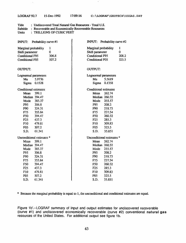
Figure 1b'.--LOGRAF summary of input and output estimates for undiscovered recoverable (curve #1) and undiscovered economically recoverable (curve #2) conventional natural gas resources of the United States. For additional output see figure 1 b.
43
D. Some Continuous Probability Distributions
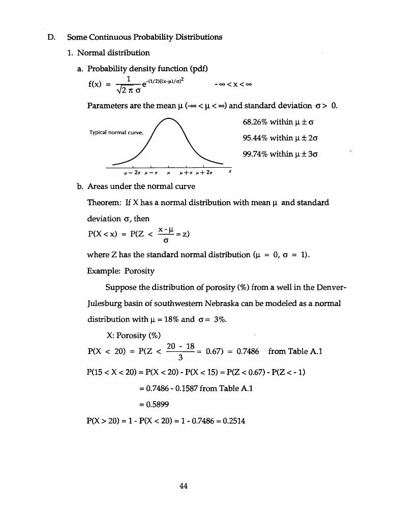
1. Normal distribution
a. Probability density function (pdf)1 2f (x) = / e - oo < x < <»
V27T a
Parameters are the mean \i (-°° < \i < °°) and standard deviation o > 0.
68.26% within u± ar x
Typical normal curve.95.44% within u±2a
99.74% within u±3o ^^
/I 2<T /I <T /I /I ~\~ <7 /I ~T" 2<T
b. Areas under the normal curve
Theorem: If X has a normal distribution with mean jj. and standard
deviation a, then
P(X<x) = P(Z < ^^ = z)a
where Z has the standard normal distribution (u = 0, a = 1).
Example: Porosity
Suppose the distribution of porosity (%) from a well in the Denver-
Julesburg basin of southwestern Nebraska can be modeled as a normal
distribution with |i = 18% and a = 3%.
X: Porosity (%)9D 18
P(X < 20) = P(Z < = 0.67) = 0.7486 from Table A.I
P(15 < X < 20) = P(X < 20) - P(X < 15) = P(Z < 0.67) - P(Z < - 1)
= 0.7486 - 0.1587 from Table A.1
= 0.5899
P(X > 20) = 1 - P(X < 20) = 1 - 0.7486 = 0.2514
44

2. PROBDIST model selection menu
Select probability distribution model for
123mm&Bi 5678910111213
Model
Probability HistogramProbability HistogramNormal
Truncated NormalLognormalTruncated LognormalExponentialTruncated ExponentialPare toTruncated ParetoUniformTriangular
Min
F100 F95FIDOF100
F100F100F100F100F100F100F100F100F100
Ave
F75 F50 F25 F5F50
MeanF50Mean (normal)
Mode
Max
FOFOFO
'^&i$8^g$8&EwiiiflHnftBiSHiWS»W5W5WW«»Jwft
FOFOFOFOFOFOFOFOFO
Shape ScaJ
ijiisisicr
er
(3
d
orLe
NOTE: F50 = Median and P ( X > F50 ) = 0.50
MOVE video bar to desired model. RETURN to select, CTRL-G to see sample graph
45

PROBDIST 89,11 FIG15.PDL 14:38:33 3-Hay-1990
Project naae : Open File ReportEstiaation naae : Test data
Units : noneModel : 7-fractile Probability Histogra§
INPUT:
VARIABLE NAME
Saaple data
OUTPUT:
VARIABLE NAME
Saaple data
PARAMETERS
Min Median MaxF100 F95 F75 F50 F25 F5 FO
0.00000 1.00000 3.00000 6.00000 14.0000 19,0000 28.0000
ESTIMATES
MEAN S. D. F100 F95 F75 F50 F25 F5 FO
8.52500 6.52745 0.00000 1.00000 3.00000 6,00000 14.0000 19.0000 28.0000
1: Sanple data
7-fractile probability histogran
0.001000 1 3.0^000 1 14^000ij 28.
1.00000 6.00000 19.0000 Any key to continue ...
000
Figure 15. Output of PROBDIST for the 7-fractile histogram model.
46

PROBDIST 89.11 PIG16.PDL 14:39:16 3-May-1990
Project naaeEstiaation naae
UnitsModel
INPUT:
VARIABLE NAME
Sanple data
OUTPUT:
VARIABLE NAME
Sanple data
Open Pile ReportTest datanone3-fractile Probability Bistogran
PARAMETERS
Hin Median Max P100 P50 PO
2. 8.00000 10.0000
ESTIMATES
HBAN S. D. P100 P95 P75 P50 P25 P5 PO
7.37916 1.75230 2,00000 4.00000 6.50000 8.00000 8.66666 9.33333 10.
1: Sanple data3-fractile probability histogran
2.00000 10.0000
4.00000 8.00000 9.33333 Any key to continue ...
Figure 16. Output of PROBDIST for the 3-fractile histogram model.
47

PROBDIST 89,11 PIG17.PDL 14:39:43 3-Maj-1990
Project naae : Open File ReportEstiiation naie : Test data
Units : noneModel : Hio/iax Nornal Distribution
INPUT:
VARIABLE NAHE
Sanple data
OUTPUT:
VARIABLE NAHE
Saaple data
PARAHETERS
Kin Max FIDO PO
2.00000 10.
ESTIMATES
MEAN S. D. P100 P95 P75 P50 P25 P5 PO
6.00000 1.46074 2.00000 3.80666 5.10000 6.00000 6.90000 8.19333 10.
1: Sanple data
M in/fiax nornal distribution
.00
S
000 5.10000\
6.90000 .i10.0000
3.80666 6.00000 8.19333 Any key to continue ...
Figure 17. Output of PROBDIST for the minimum/maximum normal distribution model.
48
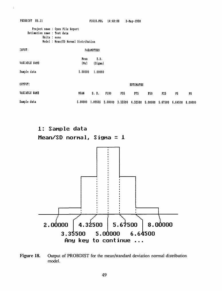
PROBDIST 89.11 PIG18.PDL 14:40:08 3-Hay-1990
Project nane : Open File ReportEstiiation Dane : Test data
Units : noneHodel : Hean/SD Nornal Distribution
INPUT:
VARIABLE NAHE
Saiple data
OUTPUT:
VARIABLE NAHE
Saiple data
PARAMETERS
Hean S.D. (Hu) (Sign)
5.00000 1.00000
ESTIMATES
HEAN S. D. P100 P95 P75 P50 P25 P5 PO
5.00000 1.09555 2.00000 3.35500 4.32500 5.00000 5.67500 6.64500 8.00000
1: Sanple data
Mean/SD nornal, Signa = 1
.0(1)000 4.32500 5.67500 1 8.00
3.3:i5QQ 5.00000 6.64500 Any key to continue ...
1000
Figure 18. Output of PROBDIST for the mean/standard deviation normal distribution model.
49

PEOBDIST 89.11 PIG19.PDL 14:40:33 3-May-1990
Project naaeBstiaation naae
UnitsModel
Open Pile ReportTest datanoneTruncated Homal Distribution
INPUT:
VARIABLE HAKE
Saaple data
OUTPUT:
VARIABLE NAME
Saaple data
PARAMETERS
Min Mean Max S.D. (FIDO) (Ma) (PO) (Signa)
2.00000 5. 10.0000 1,00000
ESTIMATES
HEAH 8, D, P100 P95 P75 P50 P25 P5 PO
5,05290 1.23119 2.00000 3.36504 4.32778 5,00163 5.67623 6.64769 10.0000
1: Sanple data
Truncated nornal, Signa =
3.36504 5.00163 6 Any key to continue ...
Figure 19. Output of PROBDIST for the truncated normal distribution model.
50
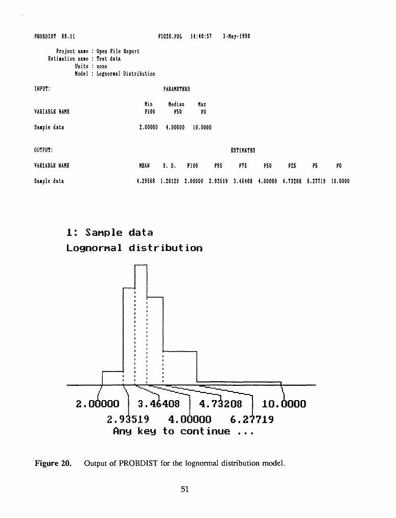
PBOBDIST 89.11 PIC20.PDL 14:40:5? 3-May-1990
Project naaeEstiaation Dane
UnitsModel
Open File Report Test datanoneLognoraal Distribution
INPUT:
VARIABLE NAME
Saiple data
OUTPUT:
VARIABLE NAME
Saiple data
PARAMETERS
Hin Median MarP100 P50 PO
2.00000 4.00000 10.0000
ESTIMATES
MEAN S. D. P100 P95 P75 P50 P25 P5 {
4.29568 1.28129 2.00000 2.93519 3.46408 4.00000 4.73208 6.27719 10,
1: Sanple data
Lognorna1 d1st r ibution
.00000 3.46408 10.0000
:519 4.00000 6.27719 Any key to continue ...
Figure 20. Output of PROBDIST for the lognormal distribution model.
51

PROBDIST 89.11 PIG21.PDL 14:41:21 3-May-1990
Project case : Open File ReportEstiaation naae : Test data
Units : noneModel : Truncated Lognoraal Distribution
IKPUT:
VARIABLE KAHE
Saaple data
OUTPUT:
VARIABLE NAME
Saaple data
PARAMETERS
Hie Noraal Mean Max S.D. P100 (Ha) FO (Signa)
2,00000 5.00000 500,000 1.20000
ESTIMATES
MEAN S. D. F100 P95 P75 P50 P25 P5 PO
158.630 125.516 2.00000 18,7198 56.6487 117.261 223.345 411.409 500.000
1: Sanple dataTruncated lognornal, Signa = 1.2
.00000 223.345 500.000
198 117.261 411.409 Any key to continue ...
Figure 21. Output of PROBDIST for the truncated lognormal distribution model.
52

PROBDIST 89.11
Project naneEstimation naae
UnitsKodel
INPUT:
VARIABLE NAME
Saiple data
OUTPUT:
VARIABLE NAME
Saiple data
PIG22.PDL 14:41:42 3-Hay-1990
Open Pile Report Test datanoneExponential Distribution
PARAMETERS
Kin Max FIDO PO
2.00000 10.0000
ESTIMATES
MEAN S. D. P100 P95 P75 P50 P25 P5 PO
3.27798 1.38289 2.00000 2.05940 2.33316 2.80274 3.60549 5.46941 10.
1: Satiple dataExponent ial distribut ion
2.00000 10.0000
2.05940 2.80274 5.46941 Any key to continue ...
Figure 22. Output of PROBDIST for the exponential distribution model.
53

PBOBDIST 89.11 PIG23.PDL 14:42:06 3-Hay-1990
Project naie : Open Pile ReportEstimation naie : Test data
Units : noneModel : Truncated Exponential Distribution
INPUT:
VARIABLE NAME
Sanple data
OUTPUT:
VARIABLE MAKE
Saiple data
PARAMETERS
Kin MaxP100 PO Beta
2.00000 10.0000 3.00000
ESTIMATES
MEAN S. D. P100 P95 P75 P50 P25 P5 PO
4,48180 2.02684 2.00000 2.14292 2.79435 3.87791 5.59086 8.46225 10,
1: Sanple data
Truncated exponential, Beta = 3
2.00000 I 2.7^435 5.59086 10.0000
2.14292 3.87791 8.46225 Any key to continue ...
Figure 23. Output of PROBDIST for the truncated exponential distribution model.
54

PEOBDIST 89.11 PIG24.PDL 14:42:35 3-Hay-1990
Project naae : Open Pile ReportEstiaation naoe : Test data
Units : noneHodel : Pareto Distribution
INPUT:
VARIABLE NAHE
Saaple data
OUTPUT:
VARIABLE NAME
Saaple data
PARAHETBRS
Kin FIDO
Har PO
ESTIMATES
MEAN S. D, FIDO F95 P75 P50 P25 F5 PO
2,74582 1.16589 2.00000 2.02404 2.13864 2.35053 2.76251 4.01936 10.
1: Sanple data
Pareto distribution
2.01 10.0000
2.02404 2.35053 4.01936 Any key to continue ...
Figure 24. Output of PROBDIST for the Pareto distribution model.
55

PBOBDIST 89.11 PIG25.PDL 14:42:56 3-Hay-1990
Project naae : Open Pile ReportBstiaation naae : Test data
Units : noneModel : Truncated Pareto Distribution
INPUT:
VARIABLE NAHB
Saaple data
OUTPUT:
VARIABLE NAHB
Saaple data
PARAMETERS
Kin MaxFIDO PO d
2.00000 10.0000 0.50000
ESTIMATES
MEAN S. D. P100 P95 P75 P50 P25 P5 PO
4.54702 2.17003 2.00000 2.11531 2.69285 3.81966 5.83592 8.86975 10.
1: Sanple data
Truncated Pareto, d = 0.5
2.00000 5.83592 10.0000
2.11531 3.81966 8.86975 Any key to continue ...
Figure 25. Output of PROBDIST for the truncated Pareto distribution model.
56

PEOBDIST 89.11 PIG26.PDL 14:43:21 3-May-1990
Project naneBstisation naae
UnitsHodel
Open Pile ReportTest datanoneUnifora Distribution
INPUT:
VARIABLE HAMB
Saaple data
OUTPUT:
VARIABLE NAME
Saaple data
PARAMETERS
Hin Har PI 00 PO
2.00000 10.0000
MEAN S. D. P100
6.00000 2.30940 2.
BSTIHATBS
P95 P75 P50 P25 P5 PO
1.40000 4.00000 6.00000 8.00000 9.60000 10.0000
1: Sample data
Uniforn distribution
2. oilOCv10 4.
"X.
oiooo 8 . 0000
.-"
^ 0 1C). 0000
2.40000 6.00000 9.6 0000 Any key to cont inue ...
Figure 26. Output of PROBDIST for the uniform distribution model.
57
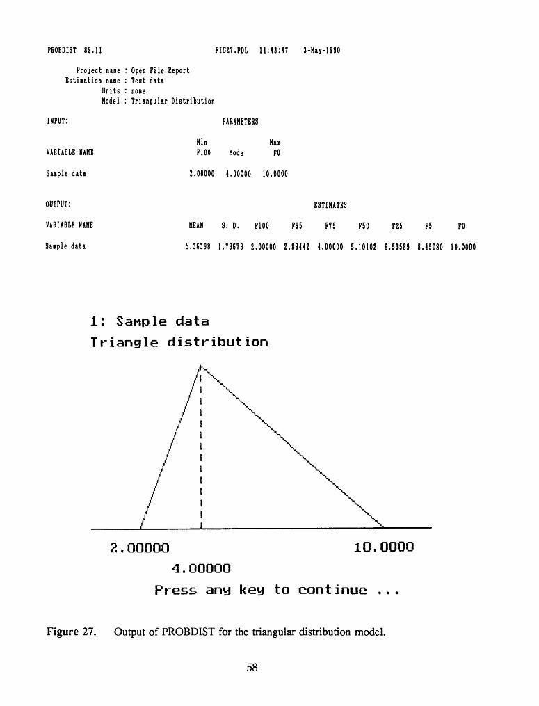
PBOBDIST 89,11
Project naneEstiaation naae
UnitsModel
INPUT:
VARIABLE NAHE
Saaple data
OUTPUT:
VARIABLE NAHE
Saaple data
PIG27.PDL 14:43:47 3-May-1990
Open Pile Report Test datanoneTriangular Distribution
PARAMETERS
HinFIDO Node
Max PO
2. 4,00000 10,
ESTIMATES
MEAN S, D. P100 P95 P75 P50 P25 P5 PO
5.36398 1,78678 2.00000 2,89442 4,00000 5,10102 6,53589 8.45080 10.0000
1: Sanple data
Triangle distribution
2.00000 10.0000
4.00000
Press any key to continue ...
Figure 27. Output of PROBDIST for the triangular distribution model.
58

59

E. Statistics
A. Sampling Concepts
1. Populations
Population of units: a set of units having some common characteristic.
Example: The population of oil fields in a play.
Population of observations: the set of all possible observations or values of a
random variable X.
A population of observations is conceptualized from a population of units if
each unit (e.g., oil field) were to be measured according to some random
variable X (e.g., oil field size).
Population distribution: the probability distribution of a random variable X
Example: Normal population means a population whose observations are
values of a random variable having a normal distribution.
Population size: the number of observations in the population.
Parent population: the population of observations that we are interested in
studying.
Example: The population of oil field sizes in a play. The parent population
distribution could be modeled as a Pareto distribution.
Sampled population: the population of observations from which a sample is
taken.
Sometimes, for various reasons (e.g., financial), the sampled population is
more restricted than the parent population.
Example: The population of oil field sizes in a play with the constraint of a
point of economic truncation. The sampled population distribution could be
modeled as a lognormal distribution.
60

uzLU
IDoLU
PARENT POPULATION
INCRUMENTAL
DISTRIBUTION
SEGIMENTS
X
"° SIZE
Figure 9.1. The progressive exhaustion of an oil and gas field size distribution by wildcat drill ing. S0 is point of economic truncation. W{ to W* are sequential segments of the field size distribution added with W{ to W* wildcat wells.
Source: Drew, 1990
61

2. Parameters
Population parameter: a parameter of the population distribution; i.e., any
numerical quantity that characterizes or describes a population
distribution.
Important: A parameter is a constant or fixed value.
Characterizing parameter: a population parameter that characterizes the
population distribution.
Descriptive parameter: a population parameter that is a function of the
characterizing parameters and describes the population distribution, e.g.,
the population mean.
Population mean: the mean (i of the population distribution.
Population variance: the variance a2 of the population distribution.
Population standard deviation: the standard deviation a of the population
distribution.
For simplicity,
"parameters" will often refer specifically to the characterizing parameters;
"moments" will refer specifically to the population mean and variance.
a. Binomial population
Population distribution: binomial distribution
Parameters:
Number of prospects: n = 3
Probability of field (success): p = 0.2
Moments:
Population mean: (i= np = (3)(0.2) = 0.6
Population variance: o2 = np(l - p) = (3)(0.2)(0.8) = 0.48
62

b. Uniform population
Population distribution: uniform distribution
Parameters:
Minimum value: a = 0
Maximum value: b = 1
Moments:a + b
Population mean: p. = =0.5
rh aY*Population variance: a2 = = 0.083
63

3. Samples
Sample: a subset of a population.
Sample size: the number of members in a sample.
Sample of units: a subset of n units from a population of units.
Example: A sample of n oil fields in a play.
Sample of observations: a subset of n observations from a sampled
population of observations, i.e., a set of n random variables Xi, X2,..., Xn.
Example: A sample of n oil field sizes in a play.
Physical sample: in geology, a single unit.
Examples: A core sample or a water sample.
Important: Unless otherwise stated, a "sample" means a sample of
observations a set of data.
Two basic types of data
Discrete data: data resulting from a discrete random variable (count data).
Example: Number of new discoveries in each of the plays making up a
basin.
Continuous data: data resulting from a continuous random variable
(measured data).
Example: Discovered oil field sizes in a play.
64

Example 1: Oil and mixed oil and gas field sizes
Oil and mixed oil and gas field sizes (in million barrels known recovery)
for 175 fields of 1 million BOE or more known recovery in the northern
Michigan Silurian reef play are given below.
Source of data is the Significant Oil and Gas Fields of the United States
Data Base, a product of NRG Associates, Inc. (1988). The version used
included discoveries up to and including 1990. Known recovery refers to
the sum of cumulative production plus reserves. Included in the NRG files
are those fields with at least 1 million BOE of known recovery and also
those smaller, but expected to eventually be revised to at least 1 million
BOE.
Let X: Oil or mixed oil and gas field size (million barrels)
65

Oil and mixed oil and gas field sizes - 1990
0.110.180.240.330.340.380.400.400.450.490.500.550.580.580.600.600.620.630.630.650.650.650.660.660.680.680.680.700.710.73
0.740.750.750.750.770.780.780.800.800.800.820.830.830.840.850.850.860.870.880.900.900.900.910.910.930.930.930.950.950.96
0.960.960.991.001.001.001.021.021.061.081.101.131.141.151.151.151.151.161.161.171.181.181.201.201.201.211.221.221.261.27
1.271.281.301.301.301.301.301.351.351.401.401.401.421.451.501.551.601.601.601.601.651.651.661.681.681.701.711.751.751.80
1.821.851.901.901.952.002.002.08 _j2.102.252.352.352.382.402.402.402.452.602.602.602.702.752.752.802.902.953.003.003.003.15
3.303.303.303.403.403.453.603.603.653.703.803.903.954.204.504.504.604.605.105.155.205.407.8012.0014.25
66
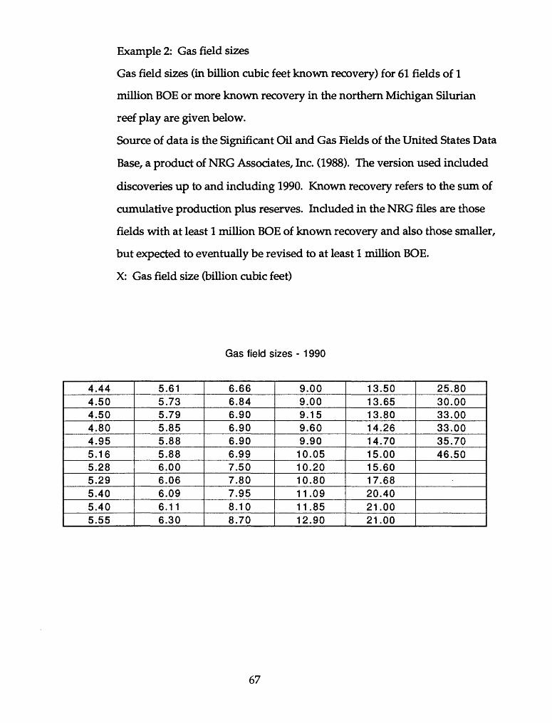
Example 2: Gas field sizes
Gas field sizes (in billion cubic feet known recovery) for 61 fields of 1
million BOB or more known recovery in the northern Michigan Silurian
reef play are given below.
Source of data is the Significant Oil and Gas Fields of the United States Data
Base, a product of NRG Associates, Inc. (1988). The version used included
discoveries up to and including 1990. Known recovery refers to the sum of
cumulative production plus reserves. Included in the NRG files are those
fields with at least 1 million BOB of known recovery and also those smaller,
but expected to eventually be revised to at least 1 million BOB.
X: Gas field size (billion cubic feet)
Gas field sizes - 1990
4.444.504.504.804.955.165.285.295.405.405.55
5.615.735.795.855.885.886.006.066.096.116.30
6.666.846.906.906.906.997.507.807.958.108.70
9.009.009.159.609.9010.0510.2010.8011.0911.8512.90
13.5013.6513.8014.2614.7015.0015.6017.6820.4021.0021.00
25.8030.0033.0033.0035.7046.50
67

Example 3: Net pay thickness data
Suppose a geologist is studying a new drilling prospect in an area in which
20 wells have been drilled. One of the unknown variables to be considered
in the new prospect is net pay thickness. To get an idea of the possible
likelihoods and ranges of possible values he has tabulated the net pay
thickness values from each of the completed wells, as shown in the table
below. Source of data is Newendorp (1975).
X: Net pay thickness (feet)
Net Pay Thickness (Feet) of 20 Wells Completed in a Basin
Well No.123456789101 1121314151617181920
Thickness111
8114259
10996
12413989
12910418665955472
16713584
154
68

4. Sampling techniques
The definitions on sampling techniques are stated in terms of observations,
but could be stated in terms of units.
Random sampling: a method of selecting a sample of size n from the
sampled population such that every possible sample of size n has an equal
chance of being selected.
Random sample: a sample that results from random sampling.
Alternatively, a set of n independent and identically distributed random
variables Xi, X2,..., Xn each having the same population distribution.
Sampling with replacement: sampling in which each observation of a
sampled population can be selected more than once.
Sampling without replacement sampling in which each observation of a
sampled population cannot be selected more than once.
Stratified random sampling: the sampled population is divided into
subpopulations and a random sample is taken from each subpopulation.
Example: A series of random samples taken independently from various
strata or depths.
Sampling proportional to size: biased sampling in which the chance of
being selected is proportional to the size of the unit.
The discovery process modeling approach suggested by Barouch and
Kaufman (1976) and Arps and Roberts (1958) relies on the following
postulates:
1. The discovery of pools within an area of exploratory interest can be
modeled statistically as sampling without replacement from an underlying
population of pools.
69

2. The discovery of a particular pool within the available population of
undiscovered pools is random with the probability of discovery being
proportional to the areal extent of the pool.
This introduces a sampling bias toward the largest pools and produces a
result where the largest pools are found more quickly.
If the sampled population is different from the parent population, then a
random sample from the sampled population will be a biased sample from
the parent population.
Parent Population
Sampled Population
Sample
70

5. Statistics
Statistic: any function of the observations comprising a sample; i.e., any
numerical quantity that is calculated from a sample Xi, X2,..., Xn. In
general, a statistic Y can be expressed in functional notation as
Y = g(X1,X2,-,Xn)
Important: A statistic is a random variable, because a function of random
variables is a random variable.
The reason the term statistic is defined so broadly, and not simply as a
numerical quantity "describing" a sample, is that in statistical inference we
calculate numerical values from the sample for the purpose of making
inferences concerning the population, and not necessarily to describe the
sample. It is important to realize that a parameter possesses a fixed value,
whereas a statistic can assume one of many possible values since it
depends on the sample; that is, the value of a statistic varies from sample to
sample.
Example: Oil and mixed oil and gas field sizes.
Oil and mixed oil and gas field sizes (in million barrels known recovery)
for 175 fields of 1 million BOE or more known recovery in the northern
Michigan Silurian reef play. Three statistics are
Minimum value: Xmin = 0-ll
Maximum value: Xmax = 14.25175
Total: £xi= 317.56
71

In summary, we are interested in the population parameters and
sample statistics (defined later) shown in the chart.
Parameters
[I population mean
O2 population variance
0 population standard deviation
Statistics
X
S2
s
sample mean
sample variance
sample standard deviation
Sampling distribution: the probability distribution of a statistic.
Example: The probability distribution of X is called the sampling
distribution of the mean.
72

B. Descriptive Statistics
1. Tabular methods
Notation: [xi, xa) means xi < x < X2
a. Frequency distribution
X:Oil or mixed oil and gas field size (million barrels)
Frequency distribution of oil and mixed oil and gas field sizes
Class Interval
1.
2.
3.
4.
5.
6.
7.
8.
9.
10.
11.
12.
[0,0.5)
[0.5, 1.0)
[1.0, 1.5)
[1.5,2.0)
[2.0,2.5)
[2.5, 3.0)
[3.0, 3.5)
[3.5, 4.0)
[4.0,4.5)
[4.5, 5.0)
[5.0, 5.5)
[5.5, 15)
Frequency f
10
53
41
21
12
9
10
7
1
4
4
_3
n = 175
73

b. Relative frequency distribution
Relative frequency distribution of oil and mixed oil and gas field sizes
Class Interval
1. [0,0.5)
2. [0.5,1.0)
3. [1.0,1.5)
4. [1.5,2.0)
5. [2.0,2.5)
6. [2.5,3.0)
7. [3.0,3.5)
8. [3.5,4.0)
9. [4.0,4.5)
10. [4.5,5.0)
11. [5.0,5.5)
12. [5.5,15)
Frequency f
10
53
41
21
12
9
10
7
1
4
4
_3
n = 175
Relative Frequency
f/n
10/175 =0.06
53/175 =0.30
41/175 =0.23
21/175 =0.12
12/175 =0.07
9/175 =0.05
10/175 =0.06
7/175 =0.04
1/175 =0.01
4/175 =0.02
4/175 =0.02
3/175 =0.02
1.00
Relative Frequency
%
6%
30%
23%
12%
7%
5%
6%
4%
1%
2%
2%
2%
100%
74
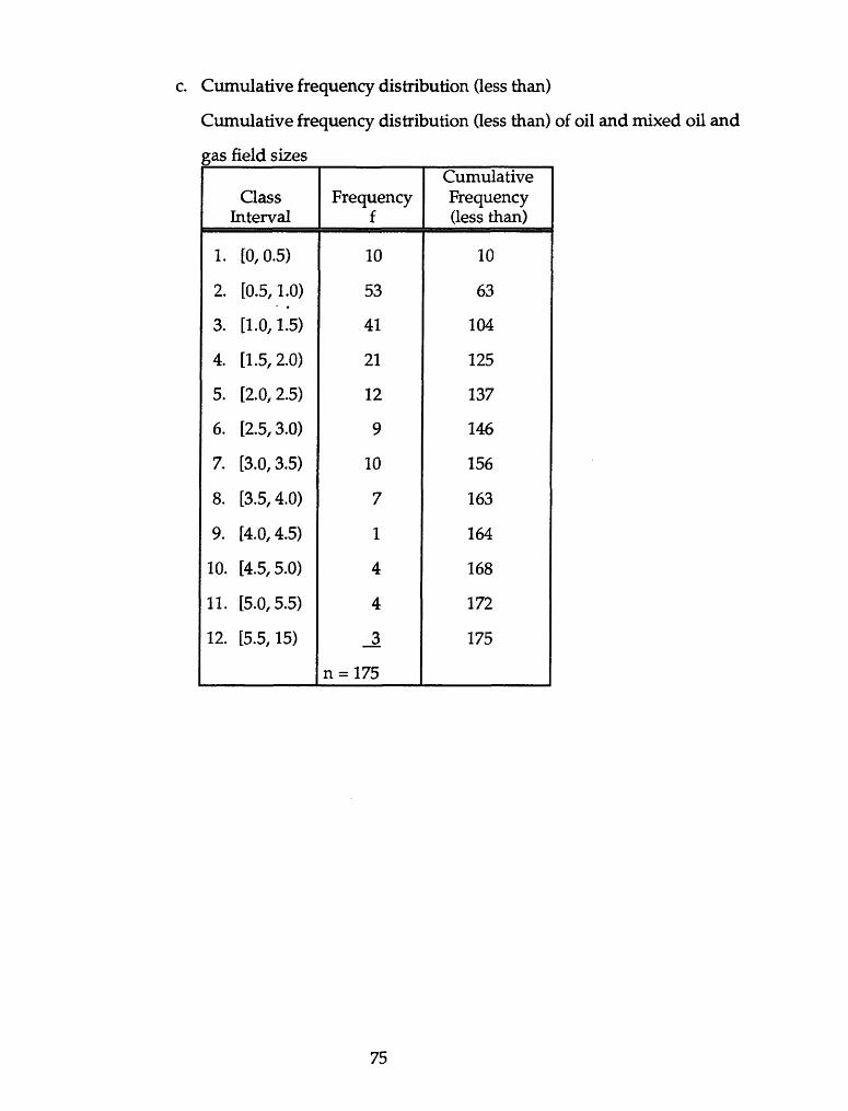
a Cumulative frequency distribution (less than)
Cumulative frequency distribution (less than) of oil and mixed oil and
gas field sizes
Class Interval
1. [0,0.5)
2. [0.5,1.0)
3. [1.0,1.5)
4. [1.5,2.0)
5. [2.0,2.5)
6. [2.5,3.0)
7. [3.0,3.5)
8. [3.5,4.0)
9. [4.0,4.5)
10. [4.5,5.0)
11. [5.0,5.5)
12. [5.5,15)
Frequency f
10
53
41
21
12
9
10
7
1
4
4
_3
n = 175
Cumulative Frequency (less than)
10
63
104
125
137
146
156
163
164
168
172
175
75

d. Relative cumulative frequency distribution (less than)
Also called cumulative proportion and cumulative percentage.
Relative cumulative frequency distribution (less than) of oil and mixed
oil and gas field sizes
Class Interval
1. [0,0.5)
2. [0.5,1.0)
3. [1.0,1.5)
4. [1.5,2.0)
5. [2.0,2.5)
6. [2.5,3.0)
7. [3.0,3.5)
8. [3.5,4.0)
9. [4.0,4.5)
10. [4.5,5.0)
11. [5.0,5.5)
12. [5.5,15)
Frequency f
10
53
41
21
12
9
10
7
1
4
4
_3
n = 175
Cumulative Frequency (less than)
10
63
104
125
137
146
156
163
164
168
172
175
Relative Cumulative Frequency Proportion
0.06
0.36
0.59
0.71
0.78
0.83
0.89
0.93
0.94
0.96
0.98
1.00
Relative Cumulative Frequency Percentage
6%
36%
59%
71%
78%
83%
89%
93%
94%
96%
98%
100%
76

e. Cumulative frequency distribution (more than)
Cumulative frequency distribution (more than) of oil and mixed oil and
gas field sizes
Class Interval
1. [0,0.5)
2. [0.5,1.0)
3. [1.0,1.5)
4. [1.5,2.0)
5. [2.0,2.5)
6. [2.5,3.0)
7. [3.0,3.5)
8. [3.5,4.0)
9. [4.0,4.5)
10. [4.5,5.0)
11. [5.0,5.5)
12. [5.5,15)
Frequency f
10
53
41
21
12
9
10
7
1
4
4
_3
n = 175
Cumulative Frequency (more than)
175
165
112
71
50
38
29
19
12
11
7
3
77

f. Relative cumulative frequency distribution (more than)
Also called cumulative proportion and cumulative percentage.
Relative cumulative frequency distribution (more than) of oil and mixed
oil and gas field sizes
Class Interval
1. [0,0.5)
2. [0.5,1.0)
3. [1.0,1.5)
4. [1.5,2.0)
5. [2.0,2.5)
6. [2.5,3.0)
7. [3.0,3.5)
8. [3.5,4.0)
9. [4.0,4.5)
10. [4.5,5.0)
11. [5.0,5.5)
12. [5.5,15)
Frequency f
10
53
41
21
12
9
10
7
1
4
4
_3
n = 175
Cumulative Frequency (more than)
175
165
112
71
50
38
29
19
12
11
7
3
Relative Cumulative Frequency Proportion
1.00
0.94
0.64
0.41
0.29
0.22
0.17
0.11
0.07
0.06
0.04
0.02
Relative Cumulative Frequency Percentage
100%
94%
64%
41%
29%
22%
' 17%
11%
7%
6%
4%
2%
78

2.
Pict
oria
l met
hods
a. F
requ
ency
his
togr
am
60
-i
50 -
40
-
ST 5=£ ;=*
so
22P
-H
20 -
10 0ITIIIIITIIIIII
08
10
11
12
13
14
15
Oil or m
ixed oil
and g
as field
size (m
illion b
arrels)

b. R
elat
ive
freq
uenc
y hi
stog
ram
0.4
-i
0.3
-
00 o
0.2
-
55
"03
0.1
-
0
0.0
2
0
I I
I T
I I
I I
I I
I I
I I
I I
I I
I
6 7
8 9
10
11
12
13
14
15
Oil or
mixed
oil and
gas fi
eld size
(millio
n barre
ls)

18
Cumulative frequency (less than)
s. o
CTQ»3 00
00 -
CT>
ps? o I"" s
o I
to8J
p
n
Iif s
OQ
f
&
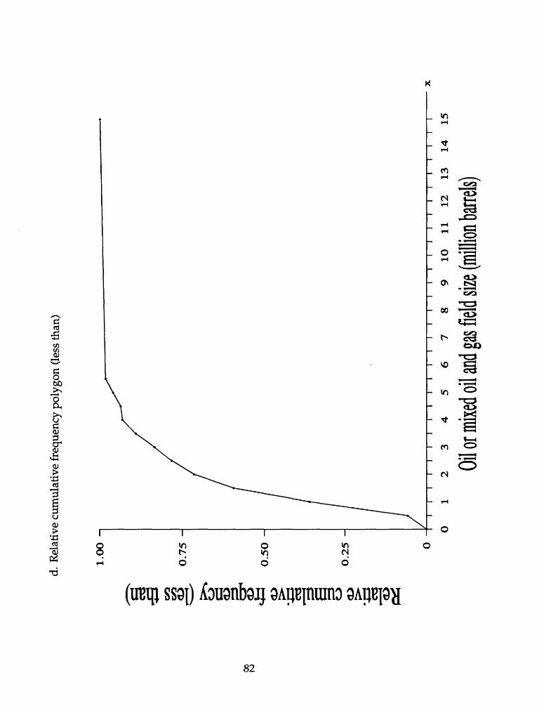
d. R
elat
ive
cum
ulat
ive
freq
uenc
y po
lygo
n (le
ss th
an)
l.OO
-i
oo NJ
a CO
C
O I Er0.7
5 -
O.5
O -
i
O.2
5 -
.£5
0i
l l
l l
l l
I l
l i
I l
l l
l I
l l
l l
l l
l l
l l
l l
r
08
10
11
12
13
14
15
Oil or
mixed
oil an
d gas
field s
ize (m
illion
barrels
)

£8
Cumulative frequency (more than)(D
ns3
I
1
3

Relative cumulative frequency (more than)p io
ON H
CP00
r O
CP
o j_
Lft
_Lcr.0>n
Iif g s
OQ O
,<
I
Ift
3. Measures of central location
Also called measures of central tendency or averages,
a. Sample mean
Definition: If Xi, X2,..., Xn represent a sample of size n, then the
sample mean is defined by the statisticn
_ IXX= i=1 n
Example 1: Net pay thickness data
X: Net pay thickness (feet)
Data from 20 wells completed in a basin:
111, 81,142,59,109,96,124,139,89,129,104,186,65,95,54,72,167,135,
84,154.
Because n = 20 and iXi = 2195,
sample mean:20
v
20 20= 109.75
Example 2: Oil and mixed oil and gas field sizes
X:Oil or mixed oil and gas field size (million barrels)
Because n = 175 and £Xi = 317.56,
sample mean:175
175 175
85

b. Sample median
Definition: If Xi, X2,..., Xn represent a sample of size n, arranged in
increasing order of magnitude, then the sample median is defined by
the statistic^ if n is odd<n /2 + X(n/2)+1 ifniseven
Example 1: Net pay thickness data
X: Net pay thickness (feet)
Arranging the 20 observations in increasing order of magnitude,
54,59,65,72,81,84,89,95,96,104,109, 111, 124,129,135,139,142,154,
167,186.
Because n = 20 is even,
sample median:X = X,0+ X,1= 104 + 109 = 106.50
2 2
Example 2: Oil and mixed oil and gas field sizes
X:Oil or mixed oil and gas field size (million barrels)
Because n = 175 is odd,
sample median:
X = X«=1.22
86

c. Sample mode
Definition: If Xi, X2,..., Xn represent a sample of size n, then the sample
mode M is that value of the sample that occurs most often or with the
maximum frequency. The mode may not exist, and when it does, it is
not necessarily unique.
Example 1: Net pay thickness data
X: Net pay thickness (feet)
Data from 20 wells completed in a basin:
111, 81,142,59,109,96,124,139,89,129,104,186,65,95,54,72,167,135,
84,154.
Because all of the values in the sample are different,
sample mode: M does not exist
Example 2: Oil and mixed oil and gas field sizes
X:Oil or mixed oil and gas field size (million barrels)
Because the value of 1.30 occurs most often with frequency of 5,
sample mode: M = 1.30
The sample mode is usually more useful in terms of a frequency
distribution, where the modal class is defined to be the class with
maximum frequency.
Modal class is [0.5,1.0)
87

4. Measures of variation
a. Sample variance
Definition: If Xi, X2,..., Xn represent a sample of size n, then the sample
variance is defined by the statistic
i=l
n-1
The reason for using n-1 as the divisor will be explained later.
Theorem:
n(n-l)
Example 1: Net pay thickness data
X: Net pay thickness (feet)
Data from 20 wells completed in a basin:
111, 81,142,59,109,96,124,139,89,129,104,186,65,95, 54, 72,167,135,
84,154.
Because n = 20, IX, = 2195 and EX? = 266531,
sample variance:g2 = 20(266531) -(2195)*
20(19)
Example 2: Oil and mixed oil and gas field sizes
X: Oil or mixed oil and gas field size (million barrels)
Because n = 175, EX, = 317.56 and EX? = 1105.62,
sample variance:C2 175(1105.62) - (317.56)2 _ n/f b = - - = o.U4
175(174)
88

b. Sample standard deviation
Definition: The sample standard deviation, denoted by S, is the positive
square root of the sample variance, i.e.,
s=Vsr
Example 1: Net pay thickness data
X: Net pay thickness (feet)
Because the sample variance S2 = 1348.93,
sample standard deviation:
S = Vl348. 93 =36.73
Example 2: Oil and mixed oil and gas field sizes
X:Oil or mixed oil and gas field size (million barrels)
Because the sample variance S2 = 3.04,
sample standard deviation:
Note: The sample standard deviation S has the same units as the
random variable X.
89

c. Sample range
Definition: If Xi, X2, ..., Xn represent a sample of size n, and X(n) and
X(D are, respectively, the largest and smallest observations in the
sample, then the sample range is defined by the statistic
R = X(n) -
Example 1: Net pay thickness data
X: Net pay thickness (feet)
Data from 20 wells completed in a basin:
111, 81, 142, 59, 109, 96, 124, 139, 89, 129, 104, 186, 65, 95, 54, 72, 167, 135,
84,154.
Because X(20) = 186 and X(i) = 54,
sample range:
R = X<20) - X(i) = 186 - 54 = 132
Example 2: Oil and mixed oil and gas field sizes
X:Oil or mixed oil and gas field size (million barrels)
Because n = 175, X(i75) = 14.25 and X(i) = 0.11,
sample range:
R = X(i75) - X(i) = 14.25 - 0.11 = 14.14
90

C. Sampling Distributions
Recall: A statistic is a random variable.
A sampling distribution is the probability distribution of a statistic.
1. Sampling distribution of the mean
a. Mean and standard deviation of X
Theorem: Given a random sample of size n from any population
with mean ji and standard deviation o, then
m = n and GJ = a / Vn
Example: Given a random sample of size n = 9 from any population of
porosity (%) with ji = 18 and o = 3, then
m = 18 and o^ = 3 / V9 = 1
b. Sampling distribution of X
Theorem: Given a random sample of size n from a normal population
with mean ji and standard deviation o, then
X has a normal distribution with p.s = \JL and o^ = o / Vn.
Therefore, P(X<x) = P(Z< x ~/^ = z)G/Vn
Example: Given a random sample of size n = 9 from a normal
population of porosity (%) with \JL = 18 and o = 3, then
X has a normal distribution with \iy = 18 and os = 1_ on _ 1 o
P(X < 20) = P(Z < = 2) = 0.9772 from Table A.1
91

Sampling distribution ofX
Population distribution
ofX
Porosity (%)
X has a normal distribution (u = 18, o = 3)
X has a normal distribution (jiy = 18, o~ = 1) for n = 9
92
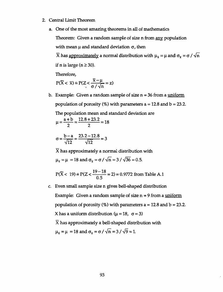
2. Central Limit Theorem
a. One of the most amazing theorems in all of mathematics
Theorem: Given a random sample of size n from any population
with mean |i and standard deviation a, then
X has approximately a normal distribution with u5 = |i and a^ = a / Vn
if n is large (n > 30).
Therefore,
P(X< x) =, a / Vn
b. Example: Given a random sample of size n = 36 from a uniform
population of porosity (%) with parameters a = 12.8 and b = 23.2.
The population mean and standard deviation are a + b 12.8 + 23.2 , 0 = is
2 2
b-a 23.2-12.8 a(J _ _=- = -a _ J
Vl2 Vl2
X has approximately a normal distribution with
(i_=(i =18 and a* = a/Vn =3/^36=0.5.
_ 1Q_1QP(X < 19) = P(Z < = 2) = 0.9772 from Table A.1
u. o
c. Even small sample size n gives bell-shaped distribution
Example: Given a random sample of size n = 9 from a uniform
population of porosity (%) with parameters a = 12.8 and b = 23.2.
X has a uniform distribution (|i = 18, a = 3)
X has approximately a bell-shaped distribution with
|i_ = |i =18 and a = a/Vn =3/V9 =1.
93

50 samples of size n = 9 from Uniform (a - 12.8, b = 23.2)
Sample1234567891011121314151617181920212223242526272829303132333435363738394041424344454647484950
X1
14.3816.6416.6816.9023.0317.8112.9912.8715.9415.1022.6722.0015.6317.0822.8115.5313.0119.1817.1219.8415.6813.4614.3115.2820.2519.9113.0215.1618.8813.3022.3414.9320.7019.0221.4415.7613.8822.9114.5815.9418.4514.2723.0621.1020.1122.2215.3717.3117.4219.50
x213.0118.4920.8318.4913.5815.9621.3519.5119.4719.5314.0513.6521.7714.2720.4620.0819.6115.0118.4517.0822.3320.5819.8416.8620.5519.5219.9920.4120.4213.0920.5113.6019.9313.0114.2121.5917.1721.4716.9620.4216.4016.6721.6314.9520.2914.0612.8915.1719.8322.30
X317.1822.0120.1216.4914.0020.4414.7522.3416.1422.9013.2721.3718.6522.1615.4521.5621.9820.6513.9516.4616.6516.9017.0518.5522.5021.3914.2513.7621.4913.2817.6816.1613.1220.9821.7821.0214.6519.8221.3720.0121.4813.3022.1818.532.1.6018.1417.8314.0915.8920.58
x421.2417.9316.2914.4317.4814.8821.0422.8615.0519.5616.2619.3521.3314.6414.4917.3820.9013.2318.6115.3514.5120.4321.2713.4814.0421.2816.1816.8214.0820.3319.5113.4822.2419.4419.0318.8113.9722.2819.9821.2423.0814.7121.2618.0314.2113.7218.7815.1519.8320.21
x521.0417.6914.9616.8013.9016.6521.3718.2022.2117.9715.0721.0716.1217.0715.0418.2715.9222.5422.9418.6514.4120.3014.4420.3421.4722.4619.6921.7519.7219.2517.1313.1113.6915.2617.2219.6021.4114.3922.4120.1415.3323.0113.5414.6414.3316.4414.4614.3216.4222.32
x613.9213.5822.8220.5422.4622.3519.5522.6616.9321.6915.7621.0414.7913.1622.0018.7213.6316.3014.8715.8221.4722.8818.7822.0517.4821.2121.5019.7717.1518.4516.4520.0617.4322.2823.1720.23
^19.2222.0115.3321.3814.3614.7613.8317.1817.6314.9618.7113.8318.8614.21
x715.6120.7818.8118.0821.6116.7513.5721.5914.7220.2519.3319.3918.9021.5513.9114.3921.3022.2321.9713.5522.9317.7720.2112.8320.0217.9718.4619.7016.3121.4516.6319.4616.1213.4922.7118.4815.0817.1622.8619.3216.8815.6516.9620.7217.0919.8720.5816.7714.1615.80
x815.6121.2717.0323.1014.2816.9719.2021.6116.8913.9221.0919.2616.9817.5717.5817.4315.1416.0417.2013.9019.7016.3621.5014.5714.8522.8818.8615.8517.9121.8019.2120.6020.3816.1619.2216.4413.8716.8714.5013.5319.9419.5920.8320.8421.8019.0919.5019.7820.0016.39
x915.8816.2914.1821.9515.0918.1021.7619.3316.4621.6622.3314.2815.0019.3416.0320.3219.4122.8415.0812.9613.6217.5519.1514.8521.7419.2422.6515.9218.4417.4614.6315.1717.0420.5618.9015.7320.9216.4921.7216.3814.6821.0019.5920.8717.2821.2418.3520.8420.1622.05
Mean16.4318.3017.9718.5317.2717.7718.4020.1117.0919.1817.7619.0517.6917.4317.5318.1917.8818.6717.8015.9517.9218.4718.5116.5319.2120.6518.2917.6818.2717.6018.2316.2917.8517.8019.7418.6316.6819.2718.8618.7117.8417.0019.2118.5418.2617.7517.3916.3618.0619.26
94
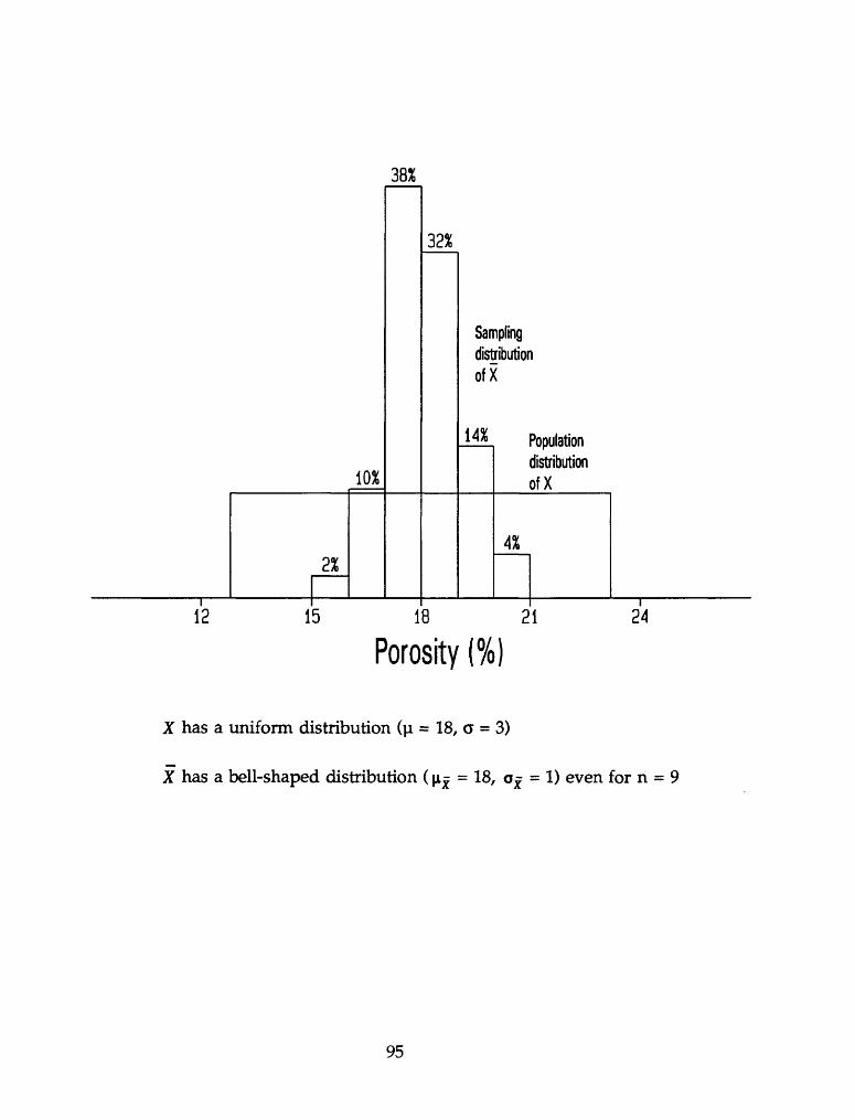
38%
10%
32%
SamplingdistributionofX
14% Population distribution ofX
12 15 18 21
Porosity (%)
X has a uniform distribution (ji = 18, a = 3)
X has a bell-shaped distribution ( \LZ = 18, o^ = 1) even for n = 9
95

3. Normal probability paper
A linear pattern of plotted points suggests a normal distribution.
50 random sample means 5EJ. with n = 9 (ji^ = 18, o^ = 1) from a uniform population (u = 18, a = 3).
Index No.
i
i23456789
1011121314151617181920212223242526272829303132333435363738394041424344454647484950
Sample Mean
*I
15.9516.2916.3616.4316.5316.6817.0017.0917.2717.3917.4317.5317.6017.6817.6917.7517.7617.7717.8017.8017.8417.8517.8817.9217.9718.0618.1918.2318.2618.2718.2918.3018.4018.4718.5118.5318.5418.6318.6718.7118.8619.0519.1819.2119.2119.2619.2719.7420.1120.65
111101181; ive Percentage
(i - 0.5)100/50
i3579
111315171921232527293133353739414345474951535557596163656769717375777981838587899193959799
96

PR
OB
AB
ILIT
Y X
90
DIV
ISIO
NS
K
EU
FF
EL
8c
ES
SE
R C
O.
MADE
IN
u.s
A.6
8000
Nor
mal
99.9
9 99
.9
99.8
99
98
95
90
80
70
60
50
40
30
20
10
5 2
1
0.5
0.2
0.1
0.05
0.
01
0.01
0.
05
0.1
0.2
0.5
1 2
5 10
20
30
40
50
60
70
80
90
95
98
99
99
.8 9
9.9
99.9
9
Cum
ulat
ive
perc
enta
ge

D. Inferential Statistics
There are two basic areas of statistics:
1. Descriptive statistics
2. Inferential statistics
Descriptive statistics: the study of techniques for describing a given set
of data.
Probability is not utilized.
Simple statistical methods are used.
e.g., pie charts, bar charts, etc.
Note: The term "descriptive statistics" is also used to refer to statistics,
e.g., the sample mean.
Inferential statistics: the study of procedures for making inferences
about a population on the basis of a sample.
Probability is utilized.
Inferences are made about aspects of a population:
1. Population distribution
e.g., normal or lognormal distribution
2. Population parameters
e.g., population mean or variance
Complex statistical methods are used:
1. Parametric statistics
2. Nonparametric statistics
Parametric statistics: statistical methods based on the assumption of a
normal population (normality assumption), and inference is made
about the population parameters, e.g., population mean ji or standard
deviation a.
98

Nonparametric (or distribution-free) statistics: statistical methods
based on no assumption of the population distribution (distribution-
free assumption).
There are two basic types of inference:
1. Statistical estimation
2. Tests of hypotheses
Statistical estimation: The type of inference is an estimate of a
population aspect.
Example: Estimate the population mean jx.
Tests of hypotheses: The type of inference is a test of hypothesis of a
population aspect.
Example: Test the hypothesis of a lognormal population.
Assumptions of a statistical method: the conditions under which the
statistical method is valid.
Robust statistical method: a statistical method that is still valid even
with moderate violation of the assumptions.
Throughout the rest of this section, a random sample is assumed.
99
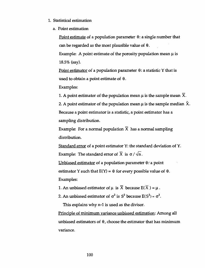
1. Statistical estimation
a. Point estimation
Point estimate of a population parameter 6: a single number that
can be regarded as the most plausible value of 6.
Example: A point estimate of the porosity population mean |i is
18.5% (say).
Point estimator of a population parameter 0: a statistic Y that is
used to obtain a point estimate of 0.
Examples:
1. A point estimator of the population mean |i is the sample mean X.
2. A point estimator of the population mean |i is the sample median X.
Because a point estimator is a statistic, a point estimator has a
sampling distribution.
Example: For a normal population X has a normal sampling
distribution.
Standard error of a point estimator Y: the standard deviation of Y.
Example: The standard error of X is c/Vn.
Unbiased estimator of a population parameter 0 r a point
estimator Y such that E(Y) = 0 for every possible value of 0.
Examples:
1. An unbiased estimator of jo, is X because E( X ) = |i.
2. An unbiased estimator of a2 is S2 because E(S2 ) = a2 .
This explains why n-1 is used as the divisor.
Principle of minimum variance unbiased estimation: Among all
unbiased estimators of 0, choose the estimator that has minimum
variance.
100

Minimum variance unbiased estimator (MVUE) of 0:
the unbiased estimator that has minimum variance.
Example: For a normal population,
1. Both X and X are unbiased estimators of the population mean
V-
2. The variance of X is smaller than the variance of X.
3. X is the MVUE of U.
Important The best estimator of jj, depends on the population
distribution.
If the population is not normal, the best estimator may not be X.
101

is an unbiased estimator of 9, while Y2 is not.
eVariance of unbiased estimator YT < variance of unbiased estimator Y,
102

b. Interval esimation
Interval estimate of a population parameter 0 : an interval of
numbers of the form yL < 6 < Vy
Example: An interval estimate of the porosity population mean u
is 17.5 < (i< 19.2 (say).
Confidence interval of a population parameter 6 : an interval such
that P(YL < 6 < YU) = 1-oc, for 0 < a < 1.
The end points YL and YU are called the lower and upper
confidence limits.
Example: A 95% confidence interval for u
Suppose that the parameter of interest is a population mean u and
the following assumptions are made
1. The population distribution is normal, and
2. The value of the population standard deviation a is known.
Recall: The sample mean X is normally distributed such that
a/Vn
has a standard normal distribution. Then
P(-1.96 < X ~|i < 1.96) = 0.95 a/Vn
Manipulating the inequalities to get the form YL < u <
P(X-1.96-S=<M-<X + 1.96-S=) = 0.95 Vn Vn
Example: A 95% confidence interval for the porosity population
mean jj, with the above assumptions and given quantities
a = 3.0, n = 16, and x = 18.5.
x±1.96-5= = 18.5±(1.96)^ = 18.5±1.5 = (17.0, 20.0) Vn V16
A 95% confidence interval for jj, is 17.0 < |J,< 20.0.
103
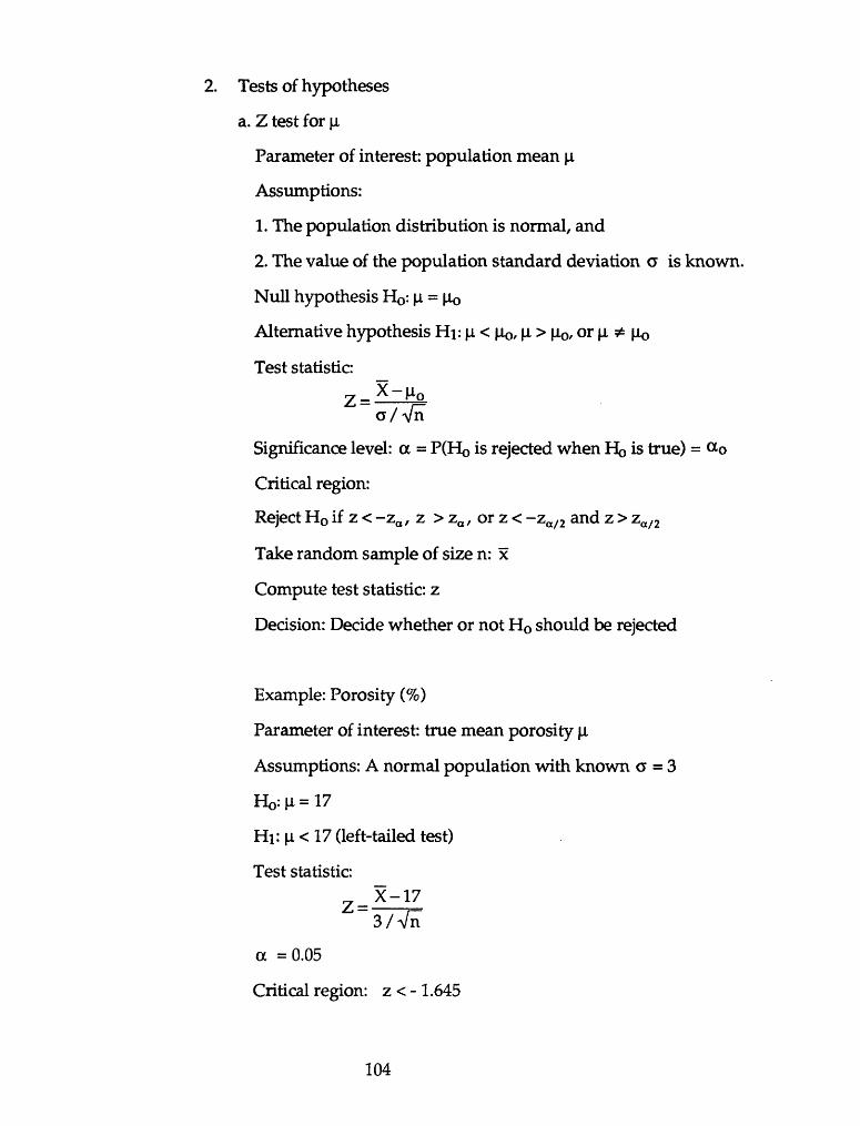
2. Tests of hypotheses
a. Z test for p,
Parameter of interest: population mean p,
Assumptions:
1. The population distribution is normal, and
2. The value of the population standard deviation a is known.
Null hypothesis HQ: p. = |io
Alternative hypothesis HI: u < |io, |i > |io/ or |i * Uo
Test statistic:
a/Vn
Significance level: a = P(Ho is rejected when HO is true) =
Critical region:
Reject H0 if z < -za/ z > za , or z < -za/2 and z > za/2
Take random sample of size n: x
Compute test statistic: z
Decision: Decide whether or not H0 should be rejected
Example: Porosity (%)
Parameter of interest: true mean porosity |i
Assumptions: A normal population with known a = 3
HI: n < 17 (left-tailed test)
Test statistic:
3/Vn"
a =0.05
Critical region: z < -1.645
104

Random sample of size n = 25 : x = 16.2
Compute: z = , = -1.33 3/V25
Decision: Do not reject HO and conclude that the mean porosity is
not significantly less than 17%.
105

b. Chi-squared goodness-of-fit test
Definition: The lognormal distribution
A nonnegative r.v. X has a lognormal distribution if
the r.v.Y = ln(X) has a normal distribution.
Parameters: mean p. and standard deviation a of the normal distribution
Example: Oil and mixed oil and gas field sizes
HQ: the population distribution is lognormal
HI: the population distribution is not lognormal
Test statistic:
where
X 2 has approximately a chi-squared distribution.
k is the number of dasses.
Fi is the observed frequency of class i.
EI = npi is the estimated expected frequency (Ei > 5 for every i).
Pi is the estimated probability of an observation falling in class i.
n is the sample size.
Significance level: a = P(Ho is rejected when HO is true) = 0.05
Critical region:
if%2 ^%a,k-l reject H0
k-l-m don't reject H0
if Xo, k-l-m < %2 < %a, k-l withhold judgment
where m is the number of independent parameters estimated.
m = 2 because \i and a are estimated from a sample.
From the sample of size n = 175, take logarithms yi = ln(xi) and
compute estimates of fi and o: y = 0.31 and s= 0.74.
106
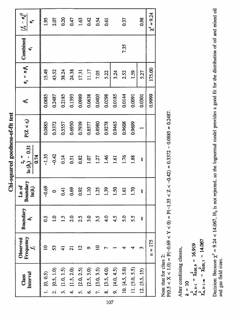
Chi
-squ
ared
goo
dnes
s-of
-fit
test
Cla
ss
Inte
rval
1. [0
,0.5
)
2.
[0.5
, 1.
0)
3.
[1.0
, 1.
5)
4.
[1.5
,2.0
)
5.
[2.0
,2.5
)
6.
[2.5
,3.0
)
7.
[3.0
,3.5
)
8.
[3.5
,4.0
)
9.
[4.0
,4.5
)
10.
[4.5
, 5.
0)
11.
[5.0
,5.5
)
12.
[5.5
, 15
)
Obs
erve
d Fr
eque
ncy
/i 10 53 41 21 12 9 10 7 1 4 4 3
n =
175
Bou
ndar
y *i 0.5 1.0
1.5
2.0
2.5
3.0
3.5
4.0
4.5
5.0
5.5
oo
Ln
of
Bou
ndar
y In
(£,)
-0.6
9
0 0.41
0.69
0.92
1.10
1.25
1.39
1.50
1.61
1.70 oo
*f =
In(^
) -
0.31
0.74
-1.3
5
-0.4
2
0.14
0.51
0.82
1.07
1.27
1.46
1.61
1.76
1.88 oo
P(Z
<z,
)
0.08
85
0.33
72
0.55
57
0.69
50
0.79
39
0.85
77
0.89
80
0.92
78
0.94
63
0.96
08
0.96
99
1
A
0.08
85
0.24
87
0.21
85
0.13
93
0.09
89
0.06
38
0.04
03
0.02
98
0.01
85
0.01
44
0.00
91
0.03
01
0.99
99
«, =
» A
15.4
9
43.5
2
38.2
4
24.3
8
17.3
1
11.1
7
7.05
5.22
3.24
2.52
1.59
5.27
175.
00
Com
bine
d*/ 7.35
(/.
- tf
et 1.95
2.07
0.20
0.47
1.63
0.42
0.54
0.61
0.37
0.98
f =
9.2
4
Not
e th
at f
or c
lass
2:
P(0.
5 <
X <
1.0
) =
P(-0
.69
< Y
< 0
) =
P(-1
.35
< Z
< -0
.42)
= 0
.337
2 -
0.08
85 =
0.2
487.
Aft
er c
ombi
ning
cla
sses
, k
= 10
X«,
*-i
= Xo
.05,9
= 16
.919
X«,
*-i-
m =
Xao5
,7 =
14.0
67
Dec
isio
n: B
ecau
se %
2 =
9.24
< 1
4.06
7, H
0 is
not r
ejec
ted,
so
the
logn
orm
al m
odel
pro
vide
s a
good
fit
for
the
dist
ribut
ion
of o
il an
d m
ixed
oil
and
gas
field
siz
es.

c. Lognormal probability paper
A linear pattern of plotted points suggests a lognormal distribution.
Example: Oil and mixed oil and gas field sizes (million barrels) for 175 fields of 1 million BOE or more known recovery in the northern Michigan Silurian reef play.
X: Oil or mixed oil and gas field size (million barrels)
108
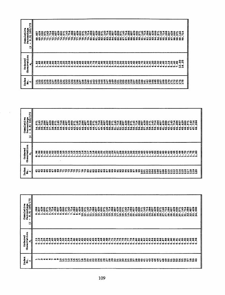
601
SB PKO g.
H
>oooooooooooooooooooooo
At*iji&ti>&>i^i^oooaB^0tCHUi«hti>(i>MOOoaBaB^uiuiui^b>i^o0a00iAinininwwK>ooa)aBuioioMooaB^b>«hOOM
IAOtOtOtOtOtOtAAOtOtOtOtOtUIMUIUIUIWMMlnUIUIMMUIUIUIUIWI«k«k«k«b«b«b«b«b«b«b«bg«b«b«k«b«bb>WWb>WWUIb>UW
/^ M In 'o '* (9 K> '^ M I* 'o W (9 ro '^ M l» <3 !h'« K> ^ M In o * (9 K> ^ M in *o '* '« K> *^ M u
S3

Lognormal Cumulative percentage1 *9 8
7
6
5
4
3
2
X-N
c 100 9
£ b00 5
W> 3
8 2
O
R '.<,7
.6
.4
.3
.2
0.1
7b :> iU ID ZU JU 4U S
..aj-iii::::::::::::::::::::::::::::::::
U DU /U OU BO _
................................«.-___-
........................ ...| ..___ _____
......... ......... .--^f !-... ...____--_
.i
Ii
U 3 D »C
(
1 1 1 1 I 1 1 1 1 1 1 II 1 1 II III 1 1 1 1 1 1 1 1 3.0 3.5 4.0 4.5 _5.0 5.5 6.0 6.5 7.0
>7b .
9
. .8
7
6
5
4
3
2
1 98
7
6
5
4
3
2
1 9
7
6
5
4
3
2
1
110

Regression and Correlation
Regression
1. Simple linear regression
Straight line
y = a + bx
where
n E xy -Zxly , - - 5 £ and a « y - bxn Ex - (Ex)
2. Simple linear regression - no constant
Straight line through origin
y = bx
where
b --2.Ex
3. Quadratic regression or polynomial regression of degree two
Parabola
The reduced major axis line
Straight line
y = a + bx
where
b = s /s = r'-^ *zj^- and a = y x \ _ 2 /r N 2 V n E x - (E x)
with b given the sign of r below.
Ill

Correlation
1. Pearson product moment correlation coefficient
n £ xy - £ x £ y_________
/[n£x2 - (£x) 2 ] [nEy2 - (£y) 2 ]
measures the strength of the linear relationship between two variables, y and x.
Nonparametric: Spearman rank correlation coefficient
2. Coefficient of Determination
2 _ SSR r ~ SST
measures what proportion of the total variation in the response y is accounted for by
the fitted regression model and is reported as a percentage AlQQ%) and interpreted
as percentage variation explained by the postulated model.
SSR is called the regression sum of squares and reflects the amount of variation in the
y values explained by the model, e.g., a postulated straight line.
SST is called the total corrected sum of squares and reflects the total amount of
variation in the y values.
112

Transformations
A function relating y to x is intrinsically linear if by means of a transformation on x and/or y, the function can be expressed as / = p0 + pjjt', where x' is the transformed independent variable and / is the transformed dependent variable.
Some useful transformations to linearize:
______ Function___________Transformation______Linear form
(a) Exponential: y - ae*x y 1 - In GO y 1 = ln(o) + p*
(b) Power: y = o* p y 1 = log GO, x' = log(*) y' = log(o) + p*'
11 /
(c) Reciprocal: y = o + p~ x 1 = - y = a + $xx x
(d) Hyperbolic: y - *a + p*
(e) Logarithmic: y = o + p log (x)
/ _ 1 / _ 1J^ > ^
y x
* 7 = log(*)
y 7 = p + a* 7
y = a + p* 7
When log (...) appears, either a base 10 or base e logarithm can be used.
113

Transformations
0<o
(a) Exponential function
0<0< 1
(b) Power function
(c) Reciprocal function
(d) Hyperbolic function
114

O-i
o
o
o
10H
I CL
LJJ
Q20H
Ro
= 0.3
7
6Z
/10
,27
9
0.4
Sour
ce: H
este
r2\
0 3.
0
VIT
RIN
ITE
RE
FLE
CT
AN
CE
(%
)5!
o

Vitrinite Ref. (X axis^ Face Cleat Spacing (Y axis')
1 0.58 1.42 0.80 0.683 0.58 1.494 0.86 0.665 0.53 1.26 0.28 4.957 0.30 3.288 1.23 0.209 0.56 0.9610 0.52 1.1711 0.55 1.0012 0.51 1.5713 0.63 0.6914 0.56 1.0415 0.47 1.0216 0.52 0.8317 0.56 1.1818 0.70 0.9019 0.79 0.5620 1.4 0.3221 1.34 0.2622 1.35 0.2323 0.69 0.4524 0.32 2.8625 0.35 2.2726 0.37 2.6427 0.36 3.3928 0.44 2.4629 0.66 1.2630 0.98 0.5531 0.79 0.9432 3.33 0.3933 3.86 0.2434 1.20 0.7835 1.58 0.4136 0.77 0.4437 0.91 0.4038 0.61 0.60
Source of data: Ben Law
116

Zlt
Face Cleat Spacing (inches)
o o
i
VO U)

An exponential relationship between face cleat spacing y and the reciprocal of vitrinite reflectance x.
y = 0.193 e°-924/x
X
0.25
0.28
0.3
0.4
0.5
0.75
1
1.5
2
2.5
3
3.5
4
y7.78
5.23
4.2
1.94
1.22
0.66
0.49
0.36
0.31
0.28
0.26
0.25
0.24
118

15 30
I I
45 60 75 90 105
EXPLORATORY FOOTAGE (MILLION FEET)
135 150
YEAR
Figure 7. Example of finding-rate curves showing extrapolation of exponential and hyperbolic curves. Historical data (data from Illinois basin) is from 1944 to 1976. The areas under the projected curves represent estimates of undiscovered recoverable oil to be found with the next 60 million feet of exploratory drilling. For the exponential curve A, the estimated amount of undiscovered recoverable oil is 0.038 billion barrels, and for the hyperbolic curve B, it is 0.115 billion barrels.
Source: Dolton and others, 1981
119

BOE IN MILLIONS0 32 B4 96128 ISO
i_____i
O ^0 ^Hm n
IE t tCD 2D
GD ID
IDZ~D
ID Or- n^o n n "nLO
O O

NO
RTH
ER
N
MIC
HIG
flN
NIf
lGflR
flN
PIN
NflC
LE
R
EE
FS
C20
0)
CU
MU
LRTI
VE
BO
E H
IST
OR
IC
MID
PO
INT
TO
TflL
0. -
2000
. 22
00. -
3000
. 22
00. H
OO
O.
EXPO
10
33.0
19
.1
21.8
HY
PER
1033
.0
66.1
106.8
400
800
1200
1600
2000
68
73
74
75
76
77
79
80
81
82
83
YE
RR
5
2400
28
00
3200
36
00
4000
CUM. EXPLOR.
DRILL
HOLE
S

NORTHERN MICHIGFiN
NIRGflRflN PI
NNfl
CLE
REEF
S (300)
CUMULf
lTIV
E BOE
HISTORIC
MIDPOINT
TOTflL
0.-
2100.
2400
.-33
00.
2400
.-42
00.
EXPO
1038.0
16.7
18.2
H
YPER
1
03
8.0
5
8.1
8
2.8
ft60
012
0016
0024
00
68
74
75
77
79
80
82
83
Y
ER
R5
3000
36
00
-120
0 48
00
5-10
0
CUM.
EX
PLOR
. DRILL
HOLES
6000

Power laws
Power laws are associated with fractals.
Power function:
Taking logarithms,
log y = log a + p log x
Obtain linear form,
/ = a' + p x'
Same line in each case:
x'
1. Both axes have arithmetic scales
2. Both axes have logarithmic scales
123
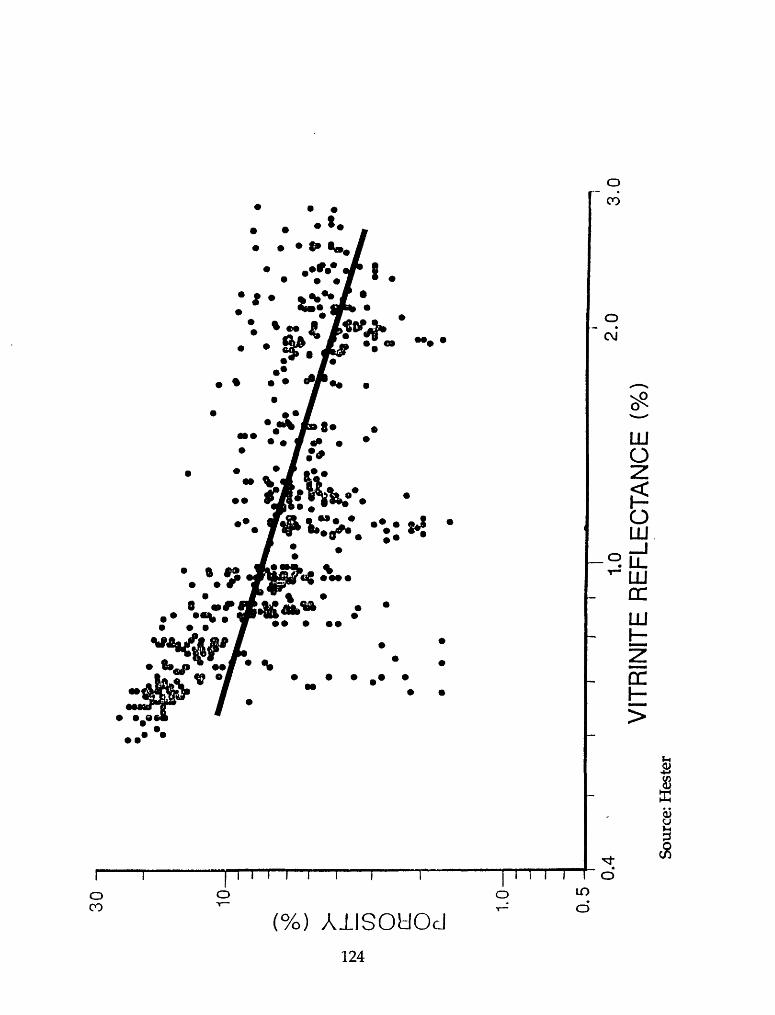
30 -i
10
-
CO O
D:
O CL
1.0
-
0.5
0.4
1.0
2.0
3.0
VIT
RIN
ITE
RE
FLE
CT
AN
CE
(%
)So
urce
: Hes
ter

e. Fractals
If the cumulative frequency distribution (more than) is plotted on log-log axes, a linear pattern of points suggests a Pareto (or fractal) distribution.
Even if the linear pattern of points is restricted to the right side of the cumulative frequency distribution due to an economic truncation, a Pareto (or fractal) distribution is suggested as a model for the parent population.
The Pareto distribution theory for this approach is established in Crovelli and Barton (submitted).
Fit a straight line to the linear pattern on the right side of the distribution.
Model: N(x) = ax* x > 0
where N(x) is the cumulative frequency distribution (more than).
125

Cumulative frequency distribution (more than) - original data of oil and mixed oil and gas field sizes
Boundary
0.110.180.240.330.340.380.400.450.490.500.550.580.600.620.630.650.660.680.700.710.730.740.750.770.780.800.820.830.840.85
0.86
0.870.880.900.910.930.950.96
Cumulative Frequency
(more than)175174173172171170169167166165164163161159158156153151148147146145144141140138135134132131
129
128127126123121118116
Boundary
0.991.001.021.061.081.101.131.141.151.161.171.181.201.211.221.261.271.281.301.351.401.421.451.501.551.601.651.661.681.70
1.71
1.751.801.821.851.901.952.00
Cumulative Frequency
(more than)113112109107106105104103102989695939089878684837876737271706965636260
59
58565554535150
Boundary
2.082.102.252.352.382.402.452.602.702.752.802.902.953.003.153.303.403.453.603.653.703.803.903.954.204.504.605.105.155.20
5.40
7.8012.0014.25
Cumulative Frequency
(more than)484746454342393835343231302926252220191716151413121197654
321
126

Cum
ulat
ive
freq
uenc
y di
strib
utio
n
1000
o
ho
^ O
§ I I O D
| OS 10
0E
10
0.1
1 10
Oil
or m
ixed
oil
and
gas
field
siz
e (m
illio
n ba
rrel
s) -
orig
inal
dat
a
100

Computation of sums for transformation of power function to linear form
B2.352.382.402.452.602.702.752.802.902.953.003.153.303.403.453.603.653.703.803.903.954.204.504.605.105.155.205.407.8012.0014.25
0
454342393835343231302926252220191716151413121 197654321
Total =
*;=logX,
0.3710.3770.3800.3890.4150.4310.4390.4470.4620.4700.4770.4980.5190.5310.5380.5560.5620.5680.5800.5910.5970.6230.6530.6630.7080.7120.7160.7320.8921.0791.154
18.132
y't = tosyt1.6531.6331.6231.5911.5801.5441.5311.5051.4911.4771.4621.4151.3981.3421.3011.2791.2301.2041.1761.1461.1141.0791.0410.9540.8450.7780.6990.6020.4770.3010.000
36.475
(40.1380.1420.1450.1510.1720.1860.1930.2000.2140.2210.2280.2480.2690.2820.2890.3090.3160.3230.3360.3490.3560.3880.4270.4390.5010.5070.5130.5360.7961.1651.331
11.670
M22.7332.6682.6352.5312.4962.3842.3452.2652.2242.1822.1392.0021.9541.8021.6931.6351.5141.4501.3831.3141.2411.1651.0840.9110.7140.6060.4890.3620.2280.0910.000
48.240
*M
0.6130.6150.6170.6190.6560.6660.6730.6730.6900.6940.6980.7050.7250.7130.7000.7110.6920.6840.6820.6770.6650.6730.6800.6320.5980.5540.5000.4410.4260.3250.00018.997
128

Computation of sums for transformation of power function to linear form
n = 31
!(*/) =18.132
11.670
36.475
48.240 18.997
b = -2.194
|b| = 2.194 is an estimate of the shape parameter of the Pareto distribution.
= 0^ = 288.246*-2.194
a' = y -bx = 2.460
= 288.246
x = 2.35, y = 44.230 x = 13, y = 1.038
V / A2 / V A II V* / A2 (V \ W > IJC I I > JC I IIM 7 IV I I > V I"ZrfV^v v^ '/ "ZrfV/iJ vZrf^;-0.981
=| 0.963
129
Selected References
Arps, J.J. and Roberts, T.G., 1958, Economics of drilling for Cretaceous oil on east flank of Denver-Julesburg Basin: American Association of Petroleum Geologists Bulletin, v. 42, p. 2549-2566.
Barouch, E. and Kaufman, G.M., 1976, Oil and gas discovery modelled as sampling without replacement and proportional to random size: Sloan School Working Paper No. 888-76.
Charpentier, R.R., 1989, A statistical analysis of the larger Silurian reefs in the northern part of the Lower Peninsula of Michigan: U.S. Geological Survey Open-File Report 89-216,34 p.
Crovelli, R.A. and Balay, R.H., 1990, PROBDIST: Probability distributions for modeling and simulation in the absence of data: U.S. Geological Survey Open-File Report 90-446-A, Documentation (paper copy) 51 p.; Open-File Report 90-446-B, Executable program (5.25" diskette).
Crovelli, R.A. and Balay, R.H., 1992, LOGRAF: Lognormal graph for resource assessment forecast: U.S. Geological Survey Open-File Report 92-679-A, Documentation (paper copy) 30 p.; Open-File Report 92-679-B, Executable program (5.25" diskette).
Crovelli, R.A. and Barton, C.C. [submitted], Fractals and the Pareto distribution applied to petroleum field-size distributions, in Barton, C.C. and LaPointe, P.R., eds., Fractal geometry and its uses in the petroleum industry: American Association of Petroleum Geologists Book Series Volume, 26 ms. p., 10 figs. (Director's approval 28-Jan-1991, and BTR log-in 26-Dec-1990.)
Crovelli, R.A., 1984, Procedures for petroleum resource assessment used by the U.S. Geological Survey statistical and probabilistic methodology, in Masters, C.D., ed., Petroleum resource assessment: International Union of Geological Sciences, pub. no. 17, p. 24-38.
Crovelli, R.A., 1984, U.S. Geological Survey probabilistic methodology for oil and gas resource appraisal of the United States: Journal of the International Association for Mathematical Geology, v. 16, no. 8, p. 797-808.
Dolton, G.L., Carlson K.H., Charpentier, R.R., Coury, A.B., Crovelli, R.A., Frezon, S.E., Khan, A.S., Lister, J.H., McMullin, R.H., Pike, R.S., Powers, R.B., Scott, E.W., and Varnes, K.L., 1981, Estimates of undiscovered recoverable conventional resources of oil and gas in the United States: U.S. Geological Survey Circular 860,87 p.
Drew, L.J., 1990, Oil and gas forecasting Reflections of a petroleum geologist: New York, Oxford University Press, International Association for Mathematical Geology, Studies in Mathematical Geology No. 2,252 p.
130

Harbaugh, J.W., Doveton, J.H., and Davis, J.C., 1977, Probability methods in oil exploration: New York, John Wiley, 269 p.
Hester, T.C., [submitted] Porosity trends of Pennsylvanian sandstones with respect to thermal maturity and thermal regimes in the Anadarko basin, Oklahoma: U.S. Geological Survey Bulletin. (Branch Chief approval and CTR log-in)
Hunter, R.L. and Mann, C.J., eds., 1992, Techniques for determining probabilities ofgeologic events and processes: New York, Oxford University Press, International Association for Mathematical Geology, Studies in Mathematical Geology, No. 4, 364 p.
Mast, R.F., Dolton, G.L., Crovelli, R.A., Root, D.H., Attanasi, E.D., Martin, P.E., Cooke, L.W., Carpenter, G.B., Pecora, W.C., and Rose, M.B., 1989, Estimates of undiscovered conventional oil and gas resources in the United States A part of the Nation's energy endowment: U.S. Geological Survey and Minerals Management Service, 44 p.
Newendorp, P.O., 1975, Decision analysis for petroleum exploration: Tulsa, Oklahoma, Petroleum Publishing Company, 668 p.
NRG Associates, Inc., 1992, The significant oil and gas fields of the United States[through December 31,1990]: Available from Nehring Associates, Inc., P.O. Box 1655, Colorado Springs, Colorado 80901.
Walpole, R.E. and Myers, R.H., 1989, Probability and statistics for engineers and scientists: New York, Macmillan Publishing Company, 4th ed., 765 p.
131

Appendix: Statistical Tables
Table A.I Areas Under the Normal Curve
z
-3.4-3.3-3.2-3.1-3.0
-2.9-2.8-2.7-2.6-2.5
-2.4-2.3-2.2-2.1-2.0
- .9- .8- .7- .6- .5
_ 4_ 3- .2-1.1-1.0
-0.9-0.8-0.7-0.6-0.5
-0.4-0.3-0.2-O.I-0.0
.00
.0003
.0005
.0007
.0010
.0013
.0019
.0026
.0035
.0047
.0062
.0082
.0107
.0139
.0179
.0228
.0287
.0359
.0446
.0548
.0668
.0808
.0968
.1151
.1357
.1587
.1841
.2119
.2420
.2743
.3085
.3446
.3821
.4207
.4602
.5000
.01
.0003
.0005
.0007
.0009
.0013
.0018
.0025
.0034
.0045
.0060
.0080
.0104
.0136
.0174
.0222
.0281
.0352
.0436
.0537
.0655
.0793
.0951
.1131
.1335
.1562
.1814
.2090
.2389
.2709
.3050
.3409
.3783
.4168
.4562
.4960
.02
.0003
.0005
.0006
.0009
.0013
.0017
.0024
.0033
.0044
.0059
.0078
.0102
.0132
.0170
.0217
.0274
.0344
.0427
.0526
.0643
.0778
.0934
.1112
.1314
.1539
.1788
.2061
.2358
.2676
.3015
.3372
.3745
.4129
.4522
.4920
.03
.0003
.0004
.0006
.0009
.0012
.0017
.0023
.0032
.0043
.0057
.0075
.0099
.0129
.0166
.0212
.0268
.0336
.0418
.0516
.0630
.0764
.0918
.1093
.1292
.1515
.1762
.2033
.2327
.2643
.2981
.3336
.3707
.4090
.4483
.4880
.04
.0003
.0004
.0006
.0008
.0012
.0016
.0023
.0031
.0041
.0055
.0073
.0096
.0125
.0162
.0207
.0262
.0329
.0409
.0505
.0618
.0749
.0901
.1075
.1271
.1492
.1736
.2005
.2296
.2611
.2946
.3300
.3669
.4052
.4443
.4840
.05
.0003
.0004
.0006
.0008
.0011
.0016
.0022
.0030
.0040
.0054
.0071
.0094
.0122
.0158
.0202
.0256
.0322
.0401
.0495
.0606
.0735
.0885
.1056
.1251
.1469
.1711
.1977
.2266
.2578
.2912
.3264
.3632
.4013
.4404
.4801
.06
.0003
.0004
.0006
.0008
.0011
.0015
.0021
.0029
.0039
.0052
.0069
.0091
.0119
.0154
.0197
.0250
.0314
.0392
.0485
.0594
.0722
.0869
.1038
.1230
.1446
.1685
.1949
.2236
.2546
.2877
.3228
.3594
.3974
.4364
.4761
.07
.0003
.0004
.0005
.0008
.0011
.0015
.0021
.0028
.0038
.0051
.0068
.0089
.0116
.0150
.0192
.0244
.0307
.0384
.0475
.0582
.0708
.0853
.1020
.1210
.1423
.1660
.1922
.2206
.2514
.2843
.3192
.3557
.3936
.4325
.4721
.08
.0003
.0004
.0005
.0007
.0010
.0014
.0020
.0027
.0037
.0049
.0066
.0087
.0113
.0146
.0188
.0239
.0301
.0375
.0465
.0571
.0694
.0838
.1003
.1190
.1401
.1635
.1894
.2177
.2483
.2810
.3156
.3520
.3897
.4286
.4681
.09
.0002
.0003
.0005
.0007'.0010
.0014
.0019
.0026
.0036
.0048
.0064
.0084
.0110
.0143
.0183
.0233
.0294
.0367
.0455
.0559
.0681
.0823
.0985
.1170
.1379
.1611
.1867
.2148
.2451
.2776
.3121
.3483
.3859
.4247
.4641
132

Appendix: Statistical Tables
Table A.I (continued) Areas Under the Normal Curve
z
0.00.10.20.30.4
0.50.60.70.80.9
.0
.1
.2
.3
.4
.5
.6
.7
.8
.9
2.02.12.22.32.4
2.52.62.72.82.9
3.03.13.23.33.4
.00
.5000
.5398
.5793
.6179
.6554
.6915
.7257
.7580
.7881
.8159
.8413
.8643
.8849
.9032
.9192
.9332
.9452
.9554
.9641
.9713
.9772
.9821
.9861
.9893
.9918
.9938
.9953
.9965
.9974
.9981
.9987
.9990
.9993
.9995
.9997
.01
.5040
.5438
.5832
.6217
.6591
.6950
.7291
.7611
.7910
.8186
.8438
.8665
.8869
.9049
.9207
.9345
.9463
.9564
.9649
.9719
.9778
.9826
.9864
.9896
.9920
.9940
.9955
.9966
.9975
.9982
.9987
.9991
.9993
.9995
.9997
.02
.5080
.5478
.5871
.6255
.6628
.6985
.7324
.7642
.7939
.8212
.8461
.8686
.8888
.9066
.9222
.9357
.9474
.9573
.9656
.9726
.9783
.9830
.9868
.9898
.9922
.9941
.9956
.9967
.9976
.9982
.9987
.9991
.9994
.9995
.9997
.03
.5120
.5517
.5910
.6293
.6664
.7019
.7357
.7673
.7967
.8238
.8485
.8708
.8907
.9082
.9236
.9370
.9484
.9582
.9664
.9732
.9788
.9834
.9871
.9901
.9925
.9943
.9957
.9968
.9977
.9983
.9988
.9991
.9994
.9996
.9997
.04
.5160
.5557
.5948
.6331
.6700
.7054
.7389
.7704
.7995
.8264
.8508
.8729
.8925
.9099
.9251
.9382
.9495
.9591
.9671
.9738
.9793
.9838
.9875
.9904
.9927
.9945
.9959
.9969
.9977
.9984
.9988
.9992
.9994
.9996
.9997
.05
.5199
.5596
.5987
.6368
.6736
.7088
.7422
.7734
.8023
.8289
.8531
.8749
.8944
.9115
.9265
.9394
.9505
.9599
.9678
.9744
.9798
.9842
.9878
.9906
.9929
.9946
.9960
.9970
.9978
.9984
.9989
.9992
.9994
.9996
.9997
.06
.5239
.5636
.6026
.6406
.6772
.7123
.7454
.7764
.8051
.8315
.8554
.8770
.8962
.9131
.9278
.9406
.9515
.9608
.9686
.9750
.9803
.9846
.9881
.9909
.9931
.9948
.9961
.9971
.9979
.9985
.9989
.9992
.9994
.9996
.9997
.07
.5279
.5675
.6064
.6443
.6808
.7157
.7486
.7794
.8078
.8340
.8577
.8790
.8980
.9147
.9292
.9418
.9525
.9616
.9693
.9756
.9808
.9850
.9884
.9911
.9932
.9949
.9962
.9972
.9979
.9985
.9989
.9992
.9995
.9996
.9997
.08
.5319
.5714
.6103
.6480
.6844
.7190
.7517
.7823
.8106
.8365
.8599
.8810
.8997
.9162
.9306
.9429
.9535
.9625
.9699
.9761
.9812
.9854
.9887
.9913
.9934
' .9951.9963.9973.9980.9986
.9990
.9993
.9995
.9996
.9997
.09
.5359
.5753
.6141
.6517
.6879
.7224
.7549
.7852
.8133
.8389
.8621
.8830
.9015
.9177
.9319
.9441
.9545
.9633
.9706
.9767
.9817
.9857
.9890
.9916
.9936
.9952
.9964
.9974
.9981
.9986
.9990
.9993
.9995
.9997
.9998
133
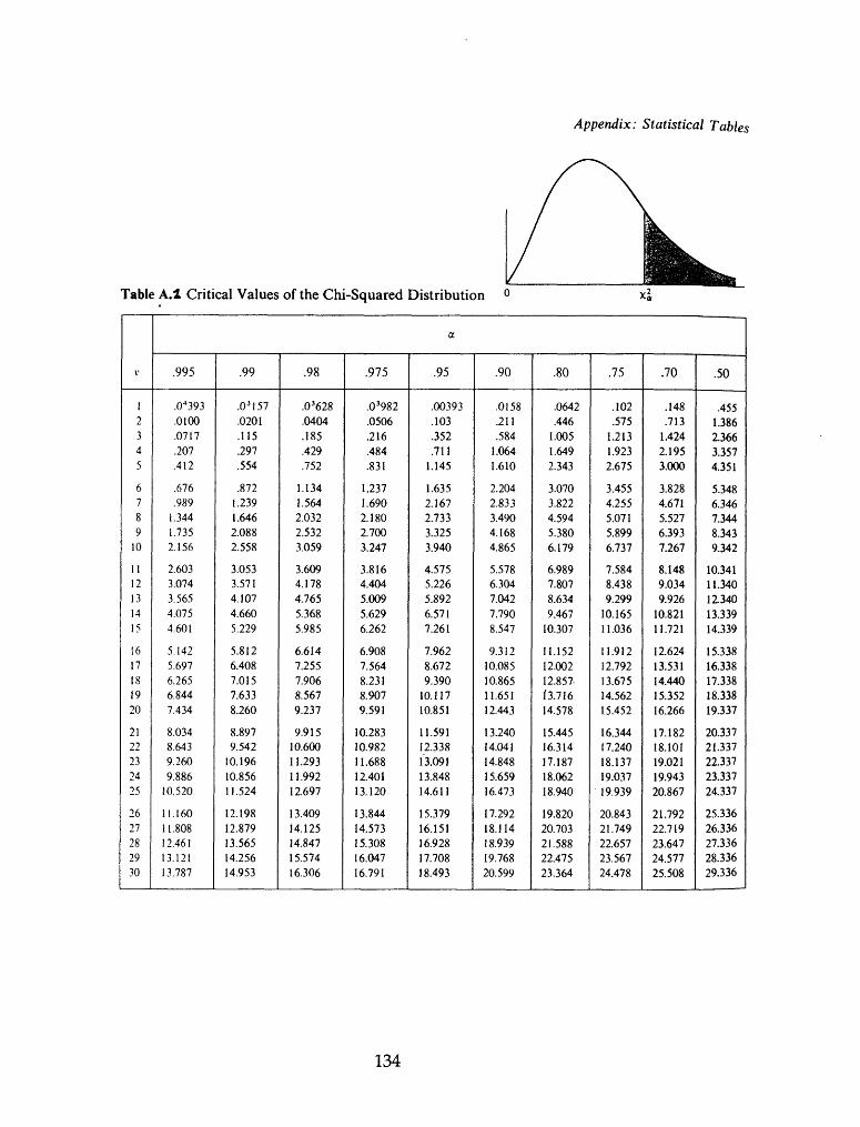
Appendix: Statistical Tables
Table A.I Critical Values of the Chi-Squared Distribution
V
12345
6789
10
1112131415
1617181920
2122232425
2627282930
a
.995
.0*393
.0100
.0717
.207
.412
.676
.9891.3441.7352.156
2.6033.0743.5654.0754.601
5.1425.6976.2656.8447.434
8.0348.6439.2609.886
10.520
11.16011.80812.46113.12113.787
.99
.0 3 157
.0201
.115
.297
.554
.8721.2391.6462.0882.558
3.0533.5714.1074.6605.229
5.8126.4087.0157.6338.260
8.8979.542
10.19610.85611.524
12.19812.87913.56514.25614.953
.98
.0 3628
.0404
.185
.429
.752
1.1341.5642.0322.5323.059
3.6094.1784.7655.3685.985
6.6147.2557.9068.5679.237
9.91510.60011.29311.99212.697
13.40914.12514.84715.57416.306
.975
.03982
.0506
.216
.484
.831
1.2371.6902.1802.7003.247
3.8164.4045.0095.6296.262
6.9087.5648.2318.9079.591
10.28310.98211.68812.40113.120
13.84414.57315.30816.04716.791
.95
.00393
.103
.352
.7111.145
1.6352.1672.7333.3253.940
4.5755.2265.8926.5717.261
7.9628.6729.390
10.11710.851
11.59112.33813.09113.84814.611
15.37916.15116.92817.70818.493
.90
.0158
.211
.5841.0641.610
2.2042.8333.4904.1684.865
5.5786.3047.0427.7908.547
9.31210.08510.86511.65112.443
13.24014.04114.84815.65916.473
17.29218.11418.93919.76820.599
.80
.0642
.4461.0051.6492.343
3.0703.8224.5945.3806.179
6.9897.8078.6349.467
10.307
11.15212.00212.857-(3.71614.578
15.44516.31417.18718.06218.940
19.82020.70321.58822.47523.364
.75
.102
.5751.2131.9232.675
3.4554.2555.0715.8996.737
7.5848.4389.299
10.16511.036
11.91212.79213.67514.56215.452
16.34417.24018.13719.03719.939
20.84321.74922.65723.56724.478
.70
.148
.7131.4242.1953.000
3.8284.6715.5276.3937.267
8.1489.0349.926
10.82111.721
12.62413.53114.44015.35216.266
17.18218.10119.02119.94320.867
21.79222.71923.64724.57725.508
.50
.4551.3862.3663.3574.351
5.3486.3467.3448.3439.342
10.34111.34012.34013.33914.339
15.33816.33817.33818.33819.337
20.33721.33722.33723.33724.337
25.33626.33627.33628.33629.336
134

Appendix: Statistical Tables
Table A.2 (continued) Critical Values of the Chi-Squared Distribution
V
12345
6789
10
1112131415
1617181920
2122232425
2627282930
a
.30"
1.0742.4083.6654.8786.064
7.2318.3839.524
10.65611.781
12.89914.01115.11916.22217.322
18.41819.51120.60121.68922.775
23.85824.93926.01827.09628.172
29.24630.31931.39132.46133.530
.25
1.3232.7734.1085.3856.626
7.8419.037
10.21911.38912.549
13.70114.84515.98417.11718.245
19.36920.48921.60522.71823.828
24.93526.03927.14128.24129.339
30.43431.52832.62033.71134.800
.20
1.6423.2194.6425.9897.289
8.5589.803
11.03012.24213.442
14.63115.81216.98518.15119.311
20.46521.61522.76023.90025.038
26.17127.30128.42929.55330.675
31.79532.91234.02735.13936.250
.10
2.7064.6056.2517.7799.236
10.64512.01713.36214.68415.987
17.27518.54919.81221.06422.307
23.54224.76925.98927.20428.412
29.61530.81332.00733.19634.382
35.56336.74137.91639.08740.256
.05
3.8415.9917.8159.488
11.070
12.59214.06715.50716.91918.307
19.67521.02622.36223.68524.996
26.29627.58728.86930.14431.410
32.67133.92435.17236.41537.652
38.88540.11341.33742.55743.773
.025
5.0247.3789.348
11.14312.832
14.44916.01317.53519.02320.483
21.92023.33724.73626.11927.488
28.84530.19131.52632.85234.170
35.47936.78138.07639.36440.646
41.92343.19444.46145.72246.979
.02
5.4127.8249.837
11.66813.388
15.03316.62218.16819.67921.161
22.61824.05425.47226.87328.259
29.63330.99532.34633.68735.020
36.34337.65938.96840.27041.566
42.85644.14045.41946.69347.962
.01
6.6359.210
11.34513.27715.086
16.81218.47520.09021.66623.209
24.72526.21727.68829.14130.578
32.00033.40934.80536.19137.566
38.93240.28941.63842.98044.314
45.64246.96348.27849.58850.892
.005
7.87910.59712.83814.86016.750
18.54820.27821.95523.58925.188
26.75728.300
.29.81931.31932.801
34.26735.71837.15638.58239.997
41.40142.79644.18145.55846.928
48.29049.64550.99352.33653.672
.001
10.82713.81516.26818.46520.517
22.45724.32226.12527.87729.588
31.26432.90934.52836.12337.697
39.25240.79042.31243.82045.315
46.79748.26849.72851.17952.620
54.05255.47656.89358.30259.703
135

Index
AAssumptions of a statistical method, 99
8Basin, 4Bayes' rule, 18Bernoulli process, 15Binomial distribution, 20,26,29,33,34,62Binomial random variable, 19
CCentral limit theorem, 93-95 Characterizing parameter, 62 Chebyshev's theorem, 34 Chi-squared goodness-of-fit test, 106,107 Combinations, 8 Combinatorial analysis
Combinations, 8Fundamental principle of counting, 8Permutations, 8
Complement of event, 7Complementary cumulative distribution function, 20,23 Conditional probability, 12 Confidence interval, 103 Continuous data, 64 Continuous probability distributions
Cumulative distribution function, 23Exponential, 53Field size, 27General graphs, 25Graphs, 24Lognormal, 51Mean/standard deviation normal, 49Minimum/maximum normal, 48Normal, 44Pareto, 55Probability density function, 23Seven-fractile histogram, 46Three-fractile histogram, 47Triangular, 58
136

Truncated exponential, 54Truncated lognormal, 52Truncated normal, 50Truncated Pareto, 56Uniform, 57Uniform (rectangular) distribution, 23,24
Continuous random variablesConcept, 22Examples, 22
Correlation, 112 Counting techniques, 8 Cumulative distribution function, 20,23 Cumulative frequency distribution (less than), 75 Cumulative frequency distribution (more than), 77 Cumulative frequency polygon (less than), 81 Cumulative frequency polygon (more than), 83
DDependence, 12,17 Descriptive parameter, 62 Descriptive parameters
Examples, 36-38Measures of central location, 29Measures of variation, 33
Descriptive statistics, 98Measures of central location, 85Measures of variation, 88Pictorial methods, 79Tabular methods, 73
Discrete data, 64 Discrete probability distributions
Binomial distribution, 20Complementary cumulative distribution, 20Cumulative distribution function, 20Graphs, 21Probability histogram, 21Probability mass function, 20
Discrete random variables, 19 Disjoint events, 7
EEvent, 5 Event relations
137
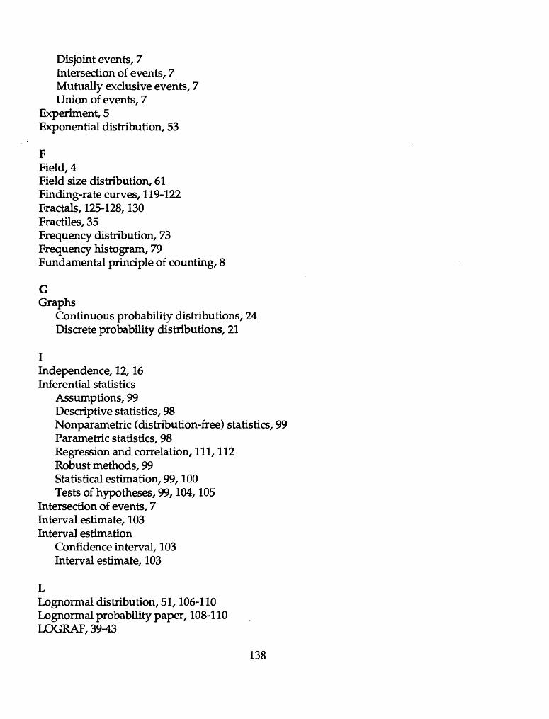
Disjoint events, 7Intersection of events, 7Mutually exdusive events, 7Union of events, 7
Experiment, 5 Exponential distribution, 53
FField, 4Field size distribution, 61Finding-rate curves, 119-122Fractals, 125-128,130Fractiles, 35Frequency distribution, 73Frequency histogram, 79Fundamental principle of counting, 8
GGraphs
Continuous probability distributions, 24 Discrete probability distributions, 21
IIndependence, 12,16 Inferential statistics
Assumptions, 99Descriptive statistics, 98Nonparametric (distribution-free) statistics, 99Parametric statistics, 98Regression and correlation, 111, 112Robust methods, 99Statistical estimation, 99,100Tests of hypotheses, 99,104,105
Intersection of events, 7 Interval estimate, 103 Interval estimation
Confidence interval, 103Interval estimate, 103
LLognormal distribution, 51,106-110 Lognormal probability paper, 108-110 LOGRAF, 39-43
138

M Mean, 29
Skewness, 32 Measures of central location
Mean, 29Median, 30Mode, 31Sample mean, 85Sample median, 86Sample mode, 87
Measures of variationSample range, 90Sample standard deviation, 89Sample variance, 88Standard deviation, 34Variance, 33
Median, 30Skewness, 32
Minimum variance unbiased estimation, 100 Mode, 31
Skewness, 32 Moments, 62 Monte Carlo simulation, 26-28
Comparison with analytic method, 28 Mutually exclusive events, 7
NNet pay thickness data, 68Nonparametric (distribution-free) statistics, 99Normal distribution
Areas under normal curve, 44Mean/standard deviation, 49Minimum/maximum, 48Probability density function, 44
Normal probability paper, 96,97
PParameters
Characterizing parameter, 62 Descriptive parameter, 62 Moments, 62 Population mean, 62 Population parameter, 62
139

Population standard deviation, 62Population variance, 62
Parametric statistics, 98 Parent population, 60 Pareto distribution, 55 Permutations, 8 Petroleum hierarchy
Basin, 4Field, 4Play, 4Pool, 4Prospect, 4Region, 4
Physical sample, 64 Pictorial methods
Cumulative frequency polygon (less than), 81Cumulative frequency polygon (more than), 83Frequency histogram, 79Relative cumulative frequency polygon (less than), 82Relative cumulative frequency polygon (more than), 84Relative frequency histogram, 80
Play, 4Point estimate, 100 Point estimation
Minimum variance unbiased estimation, 100Minimum variance unbiased estimator, 101,102Point estimate, 100Point estimator, 100Standard error, 100Unbiased estimator, 100
Point estimator, 100 Pool, 4Population distribution, 60 Population mean, 62 Population of observations, 60 Population of units, 60 Population parameter, 62 Population size, 60 Population standard deviation, 62 Population variance, 62 Populations
Parent population, 60Population distribution, 60Population of observations, 60
140
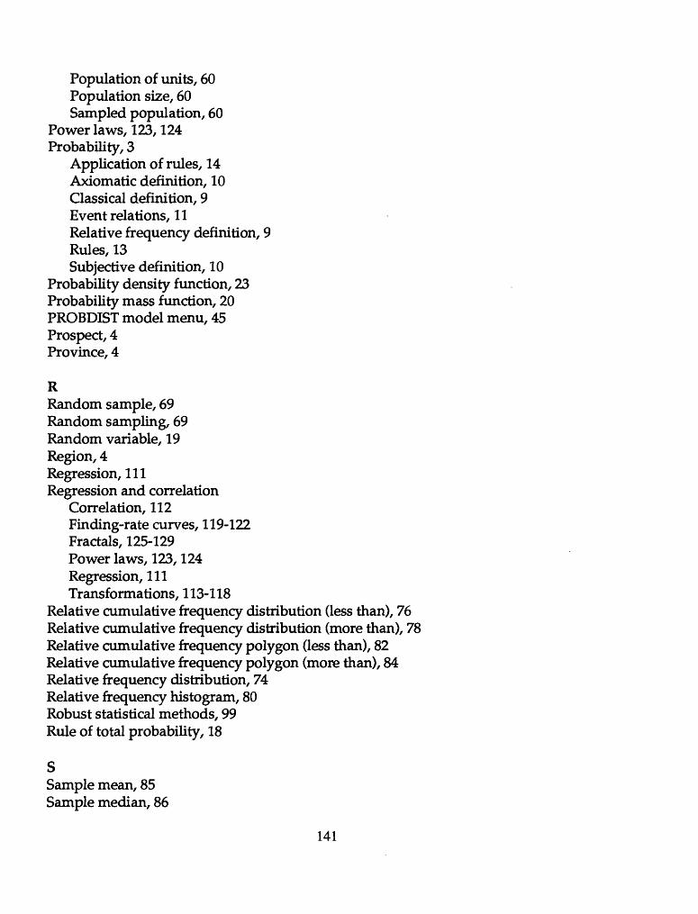
Population of units, 60Population size, 60Sampled population, 60
Power laws, 123,124 Probability, 3
Application of rules, 14Axiomatic definition, 10Classical definition, 9Event relations, 11Relative frequency definition, 9Rules, 13Subjective definition, 10
Probability density function, 23 Probability mass function, 20 PROBDIST model menu, 45 Prospect, 4 Province, 4
RRandom sample, 69 Random sampling, 69 Random variable, 19 Region, 4 Regression, 111 Regression and correlation
Correlation, 112Finding-rate curves, 119-122Fractals, 125-129Power laws, 123,124Regression, 111Transformations, 113-118
Relative cumulative frequency distribution (less than), 76 Relative cumulative frequency distribution (more than), 78 Relative cumulative frequency polygon (less than), 82 Relative cumulative frequency polygon (more than), 84 Relative frequency distribution, 74 Relative frequency histogram, 80 Robust statistical methods, 99 Rule of total probability, 18
SSample mean, 85 Sample median, 86
141

Sample mode, 87Sample of observations, 64Sample of units, 64Sample range, 90Sample size, 64Sample space, 5Sample standard deviation, 89Sampled population, 60Samples
Continuous data, 64Discrete data, 64Gas field sizes, 67Oil field sizes, 65,66Physical sample, 64Sample of observations, 64Sample of units, 64Sample size, 64
Sampling conceptsParameters, 62,72Populations, 60Samples, 64Sampling techniques, 69Statistics, 71,72
Sampling distribution of the mean, 91,92 Sampling distributions, 72
Central limit theorem, 93-95Normal probability paper, 96,97Sampling distribution of the mean, 91,92
Sampling proportional to size, 69 Sampling techniques
Biased sampling, 70Random sample, 69Random sampling, 69Sampling proportional to size, 69Sampling with replacement, 69Sampling without replacement, 69Stratified random sampling, 69
Sampling with replacement, 69 Sampling without replacement, 69 Seven-fractile histogram, 46 Skewness, 32 Standard deviation, 34 Standard error, 100 Statistic, 71
142
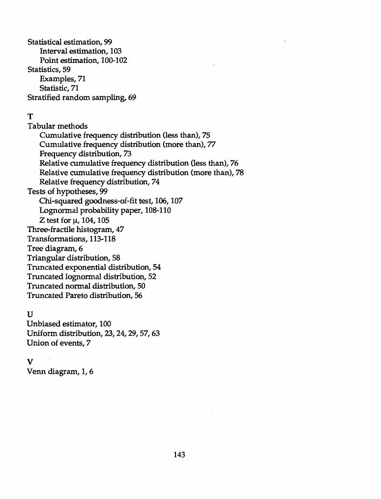
Statistical estimation, 99Interval estimation, 103Point estimation, 100-102
Statistics, 59Examples, 71Statistic, 71
Stratified random sampling, 69
TTabular methods
Cumulative frequency distribution (less than), 75Cumulative frequency distribution (more than), 77Frequency distribution, 73Relative cumulative frequency distribution (less than), 76Relative cumulative frequency distribution (more than), 78Relative frequency distribution, 74
Tests of hypotheses, 99Chi-squared goodness-of-fit test, 106,107Lognormal probability paper, 108-110Z test for u, 104,105
Three-fractile histogram, 47 Transformations, 113-118 Tree diagram, 6 Triangular distribution, 58 Truncated exponential distribution, 54 Truncated lognormal distribution, 52 Truncated normal distribution, 50 Truncated Pareto distribution, 56
UUnbiased estimator, 100Uniform distribution, 23,24,29,57,63Union of events, 7
VVenn diagram, 1,6
143