Embed Size (px)
Citation preview
Probability
Assignment
Uson, Adriana Co
CHAPTER 4
Exercise 4.48
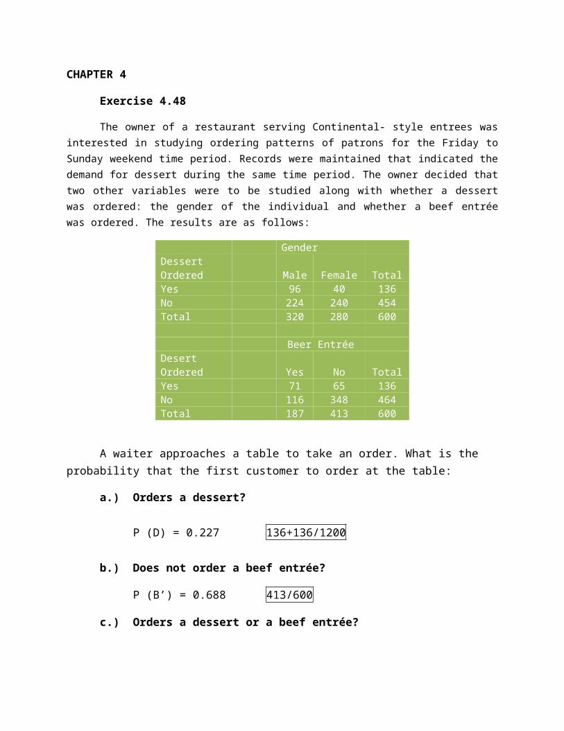
The owner of a restaurant serving Continental- style entrees was interested in studying ordering patterns of patrons for the Friday to Sunday weekend time period. Records were maintained that indicated the demand for dessert during the same time period. The owner decided that two other variables were to be studied along with whether a dessert was ordered: the gender of the individual and whether a beef entrée was ordered. The results are as follows:
Gender Dessert Ordered Male Female TotalYes 96 40 136No 224 240 454Total 320 280 600 Beer EntréeDesert Ordered Yes No TotalYes 71 65 136No 116 348 464Total 187 413 600
A waiter approaches a table to take an order. What is the probability that the first customer to order at the table:
a.) Orders a dessert?
P (D) = 0.227 136+136/1200
b.) Does not order a beef entrée?
P (B’) = 0.688 413/600
c.) Orders a dessert or a beef entrée?
P (D or B) = 0.42 136+187-71/600
d.) Is a female and does not order a dessert?
P (F and D’) = 0.40 240/600
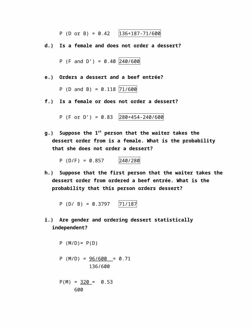
e.) Orders a dessert and a beef entrée?
P (D and B) = 0.118 71/600
f.) Is a female or does not order a dessert?
P (F or D’) = 0.83 280+454-240/600
g.) Suppose the 1st person that the waiter takes the dessert order from is a female. What is the probability that she does not order a dessert?
P (D/F) = 0.857 240/280
h.) Suppose that the first person that the waiter takes the dessert order from ordered a beef entrée. What is the probability that this person orders dessert?
P (D/ B) = 0.3797 71/187
i.) Are gender and ordering dessert statistically independent?
P (M/D)= P(D)
P (M/D) = 96/600 = 0.71 136/600
P(M) = 320 = 0.53600
No. Gender and ordering of dessert are not statistically independent because P (M/D) is not equal to P (D).
j.) Is ordering a beef entrée statistically independent of whether the person orders dessert?
P (B/D) = P (B)P (B/D) = 71/600 = 0.52
136/600P (B) = 187 = 0.312 600
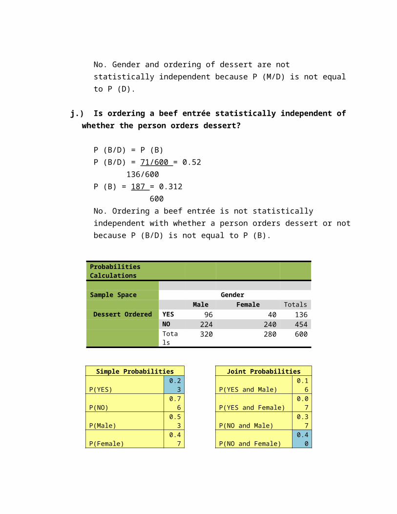
No. Ordering a beef entrée is not statistically independent with whether a person orders dessert or not because P (B/D) is not equal to P (B).
Probabilities Calculations
Sample Space Gender Male Female Totals
Dessert Ordered YES 96 40 136 NO 224 240 454
Totals 320 280 600
Simple Probabilities Joint ProbabilitiesP(YES) 0.23 P(YES and Male) 0.16P(NO) 0.76 P(YES and Female) 0.07P(Male) 0.53 P(NO and Male) 0.37P(Female) 0.47 P(NO and Female) 0.40
Addition RuleP(YES or Male) 0.60P(YES or Female) 0.63P(NO or Male) 0.92P(NO or Female) 0.82
Probabilities Calculations
Sample Space Beef Entrée YES B NO B Totals
Dessert YES D 71 65 136 NO D 116 348 464
Totals 187 413 600
Simple Probabilities Joint ProbabilitiesP(YES D) 0.23 P(YES D and YES B) 0.12P(NO D) 0.77 P(YES D and NO B) 0.11P(YES B) 0.31 P(NO D and YES B) 0.19P(NO B) 0.69 P(NO D and NO B) 0.58
Addition RuleP(YES D or YES B) 0.42
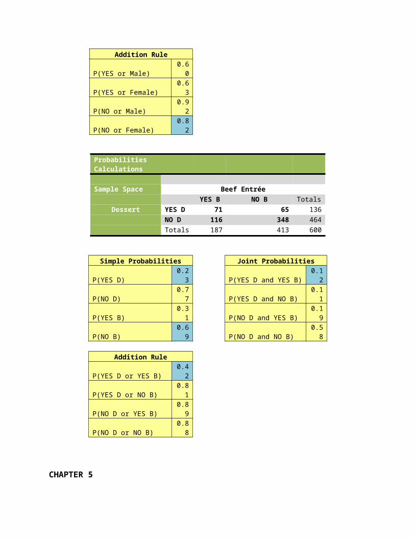
P(YES D or NO B) 0.81P(NO D or YES B) 0.89P(NO D or NO B) 0.88
CHAPTER 5
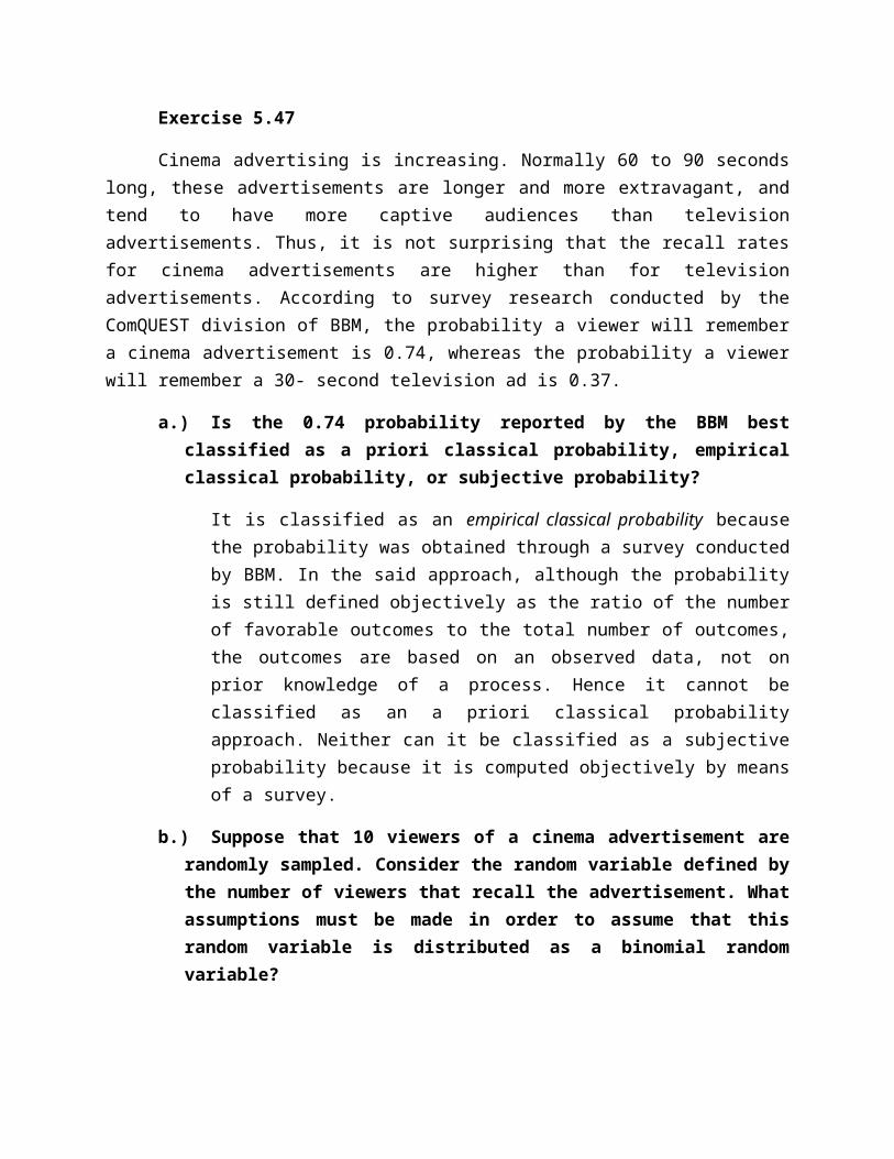
Exercise 5.47
Cinema advertising is increasing. Normally 60 to 90 seconds long, these advertisements are longer and more extravagant, and tend to have more captive audiences than television advertisements. Thus, it is not surprising that the recall rates for cinema advertisements are higher than for television advertisements. According to survey research conducted by the ComQUEST division of BBM, the probability a viewer will remember a cinema advertisement is 0.74, whereas the probability a viewer will remember a 30- second television ad is 0.37.
a.) Is the 0.74 probability reported by the BBM best classified as a priori classical probability, empirical classical probability, or subjective probability?
It is classified as an empirical classical probability because the probability was obtained through a survey conducted by BBM. In the said approach, although the probability is still defined objectively as the ratio of the number of favorable outcomes to the total number of outcomes, the outcomes are based on an observed data, not on prior knowledge of a process. Hence it cannot be classified as an a priori classical probability approach. Neither can it be classified as a subjective probability because it is computed objectively by means of a survey.
b.) Suppose that 10 viewers of a cinema advertisement are randomly sampled. Consider the random variable defined by the number of viewers that recall the advertisement. What assumptions must be made in order to assume that this random variable is distributed as a binomial random variable?
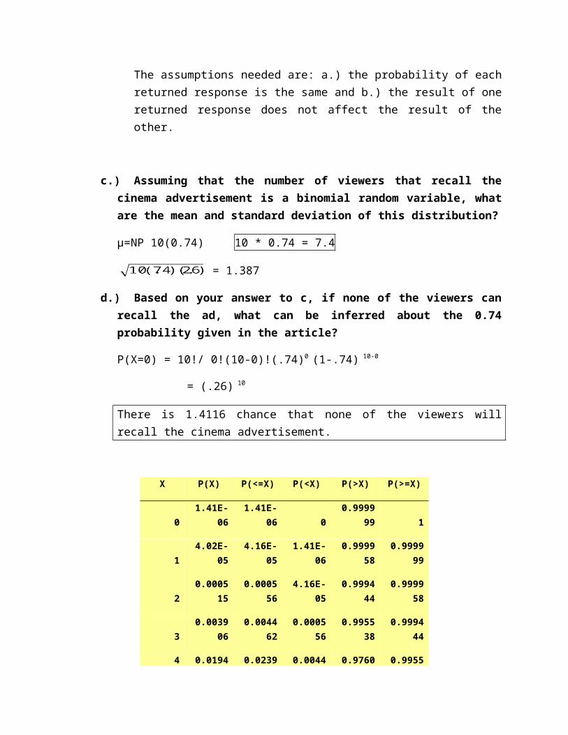
The assumptions needed are: a.) the probability of each returned response is the same and b.) the result of one returned response does not affect the result of the other.
c.) Assuming that the number of viewers that recall the cinema advertisement is a binomial random variable, what are the mean and standard deviation of this distribution?
µ=NP 10(0.74) 10 * 0.74 = 7.4
= 1.387
d.) Based on your answer to c, if none of the viewers can recall the ad, what can be inferred about the 0.74 probability given in the article?
P(X=0) = 10!/ 0!(10-0)!(.74)0 (1-.74) 10-0
= (.26) 10
There is 1.4116 chance that none of the viewers will recall the cinema advertisement.
X P(X) P(<=X) P(<X) P(>X) P(>=X)
0 1.41E-06 1.41E-06 0 0.999999 1
1 4.02E-05 4.16E-05 1.41E-06 0.999958 0.999999
2 0.000515 0.000556 4.16E-05 0.999444 0.999958
3 0.003906 0.004462 0.000556 0.995538 0.999444
4 0.019453 0.023915 0.004462 0.976085 0.995538
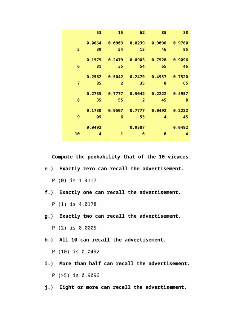
5 0.066439 0.090354 0.023915 0.909646 0.976085
6 0.157581 0.247935 0.090354 0.752065 0.909646
7 0.256285 0.50422 0.247935 0.49578 0.752065
8 0.273535 0.777755 0.50422 0.222245 0.49578
9 0.173005 0.95076 0.777755 0.04924 0.222245
10 0.04924 1 0.95076 0 0.04924
Compute the probability that of the 10 viewers:
e.) Exactly zero can recall the advertisement.
P (0) is 1.4117
f.) Exactly one can recall the advertisement.
P (1) is 4.0178
g.) Exactly two can recall the advertisement.
P (2) is 0.0005
h.) All 10 can recall the advertisement.
P (10) is 0.0492
i.) More than half can recall the advertisement.
P (>5) is 0.9096
j.) Eight or more can recall the advertisement.
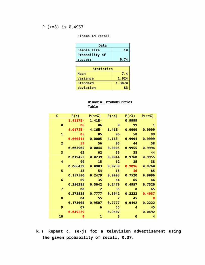
P (>=8) is 0.4957
Cinema Ad Recall
DataSample size 10Probability of success 0.74
StatisticsMean 7.4Variance 1.924Standard deviation 1.387083
Binomial Probabilities Table
X P(X) P(<=X) P(<X) P(>X) P(>=X)0 1.4117E-06 1.41E-06 0 0.999999 11 4.0178E-05 4.16E-05 1.41E-06 0.999958 0.9999992 0.00051459 0.000556 4.16E-05 0.999444 0.9999583 0.00390562 0.004462 0.000556 0.995538 0.9994444 0.01945299 0.023915 0.004462 0.976085 0.9955385 0.06643943 0.090354 0.023915 0.909646 0.9760856 0.15758069 0.247935 0.090354 0.752065 0.9096467 0.25628508 0.50422 0.247935 0.49578 0.7520658 0.27353504 0.777755 0.50422 0.222245 0.495789 0.17300507 0.95076 0.777755 0.04924 0.222245
10 0.0492399 1 0.95076 0 0.04924
k.) Repeat c, (e-j) for a television advertisement using the given probability of recall, 0.37.
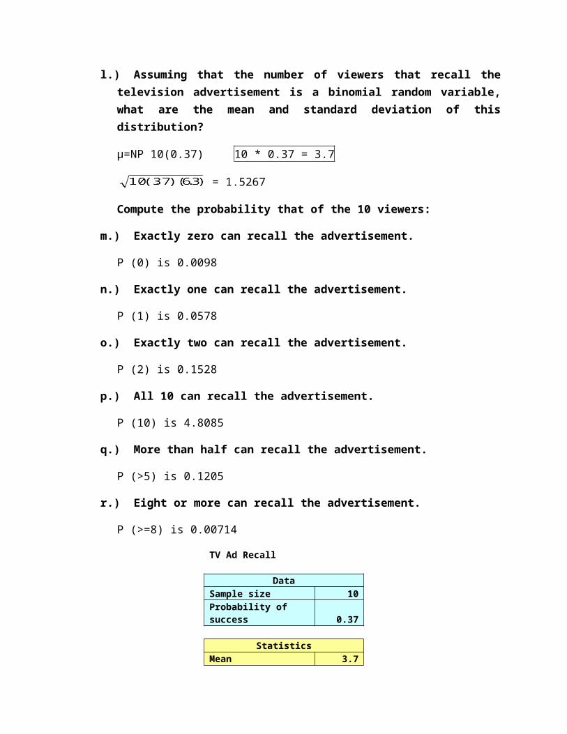
l.) Assuming that the number of viewers that recall the television advertisement is a binomial random variable, what are the mean and standard deviation of this distribution?
µ=NP 10(0.37) 10 * 0.37 = 3.7
= 1.5267
Compute the probability that of the 10 viewers:
m.) Exactly zero can recall the advertisement.
P (0) is 0.0098
n.) Exactly one can recall the advertisement.
P (1) is 0.0578
o.) Exactly two can recall the advertisement.
P (2) is 0.1528
p.) All 10 can recall the advertisement.
P (10) is 4.8085
q.) More than half can recall the advertisement.
P (>5) is 0.1205
r.) Eight or more can recall the advertisement.
P (>=8) is 0.00714
TV Ad Recall
DataSample size 10Probability of success 0.37
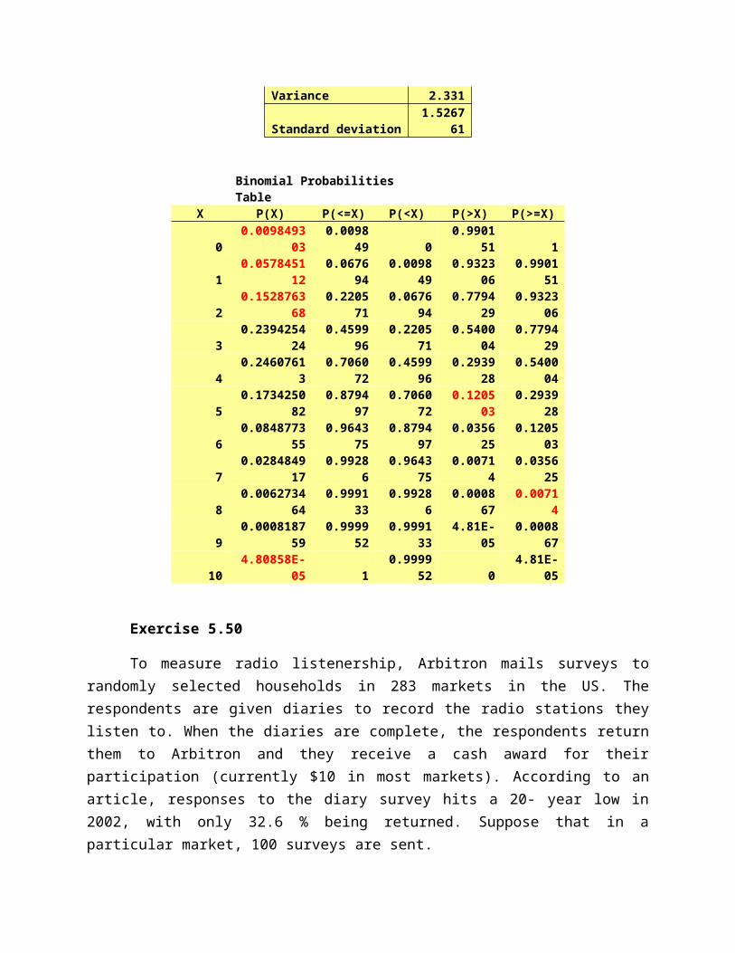
StatisticsMean 3.7Variance 2.331Standard deviation 1.526761
Binomial Probabilities TableX P(X) P(<=X) P(<X) P(>X) P(>=X)
0 0.009849303 0.009849 0 0.990151 11 0.057845112 0.067694 0.009849 0.932306 0.9901512 0.152876368 0.220571 0.067694 0.779429 0.9323063 0.239425424 0.459996 0.220571 0.540004 0.7794294 0.24607613 0.706072 0.459996 0.293928 0.5400045 0.173425082 0.879497 0.706072 0.120503 0.2939286 0.084877355 0.964375 0.879497 0.035625 0.1205037 0.028484917 0.99286 0.964375 0.00714 0.0356258 0.006273464 0.999133 0.99286 0.000867 0.007149 0.000818759 0.999952 0.999133 4.81E-05 0.000867
10 4.80858E-05 1 0.999952 0 4.81E-05
Exercise 5.50
To measure radio listenership, Arbitron mails surveys to randomly selected households in 283 markets in the US. The respondents are given diaries to record the radio stations they listen to. When the diaries are complete, the respondents return them to Arbitron and they receive a cash award for their participation (currently $10 in most markets). According to an article, responses to the diary survey hits a 20- year low in 2002, with only 32.6 % being returned. Suppose that in a particular market, 100 surveys are sent.
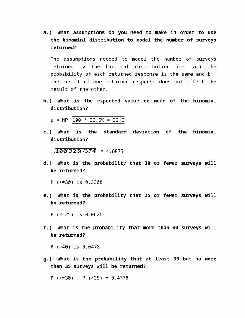
a.) What assumptions do you need to make in order to use the binomial distribution to model the number of surveys returned?
The assumptions needed to model the number of surveys returned by the binomial distribution are: a.) the probability of each returned response is the same and b.) the result of one returned response does not affect the result of the other.
b.) What is the expected value or mean of the binomial distribution?
µ = NP 100 * 32.6% = 32.6
c.) What is the standard deviation of the binomial distribution?
= 4.6875
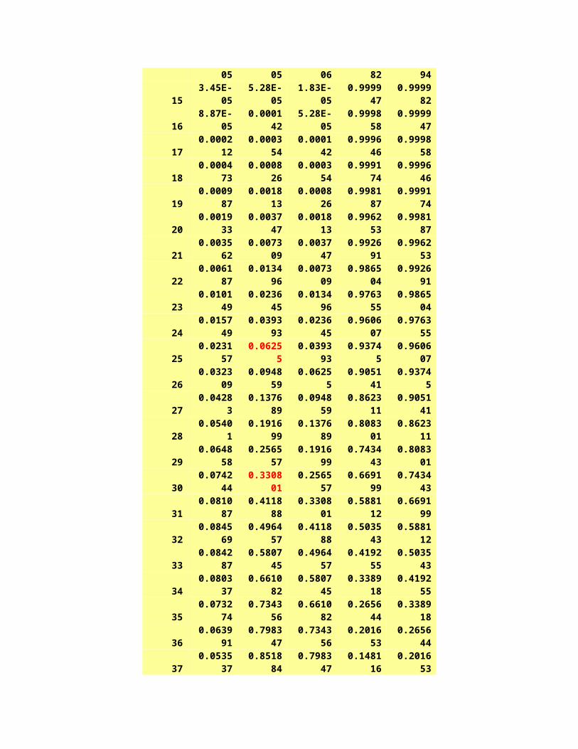
d.) What is the probability that 30 or fewer surveys will be returned?
P (<=30) is 0.3308
e.) What is the probability that 25 or fewer surveys will be returned?
P (<=25) is 0.0626
f.) What is the probability that more than 40 surveys will be returned?
P (>40) is 0.0478
g.) What is the probability that at least 30 but no more than 35 surveys will be returned?
P (>=30) – P (>35) = 0.4778
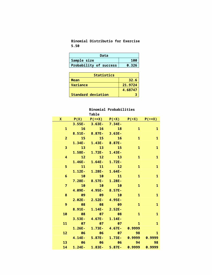
Binomial Distributio for Exercise 5.50
DataSample size 100Probability of success 0.326
StatisticsMean 32.6Variance 21.9724Standard deviation 4.687473
Binomial Probabilities TableX P(X) P(<=X) P(<X) P(>X) P(>=X)
1 3.55E-16 3.63E-16 7.34E-18 1 12 8.51E-15 8.87E-15 3.63E-16 1 13 1.34E-13 1.43E-13 8.87E-15 1 14 1.58E-12 1.72E-12 1.43E-13 1 15 1.46E-11 1.64E-11 1.72E-12 1 16 1.12E-10 1.28E-10 1.64E-11 1 17 7.28E-10 8.57E-10 1.28E-10 1 18 4.09E-09 4.95E-09 8.57E-10 1 19 2.02E-08 2.52E-08 4.95E-09 1 1
10 8.91E-08 1.14E-07 2.52E-08 1 111 3.53E-07 4.67E-07 1.14E-07 1 112 1.26E-06 1.73E-06 4.67E-07 0.999998 113 4.14E-06 5.87E-06 1.73E-06 0.999994 0.99999814 1.24E-05 1.83E-05 5.87E-06 0.999982 0.99999415 3.45E-05 5.28E-05 1.83E-05 0.999947 0.99998216 8.87E-05 0.000142 5.28E-05 0.999858 0.99994717 0.000212 0.000354 0.000142 0.999646 0.99985818 0.000473 0.000826 0.000354 0.999174 0.99964619 0.000987 0.001813 0.000826 0.998187 0.99917420 0.001933 0.003747 0.001813 0.996253 0.99818721 0.003562 0.007309 0.003747 0.992691 0.99625322 0.006187 0.013496 0.007309 0.986504 0.99269123 0.010149 0.023645 0.013496 0.976355 0.98650424 0.015749 0.039393 0.023645 0.960607 0.97635525 0.023157 0.06255 0.039393 0.93745 0.96060726 0.032309 0.094859 0.06255 0.905141 0.93745
27 0.04283 0.137689 0.094859 0.862311 0.90514128 0.05401 0.191699 0.137689 0.808301 0.86231129 0.064858 0.256557 0.191699 0.743443 0.80830130 0.074244 0.330801 0.256557 0.669199 0.74344331 0.081087 0.411888 0.330801 0.588112 0.66919932 0.084569 0.496457 0.411888 0.503543 0.58811233 0.084287 0.580745 0.496457 0.419255 0.50354334 0.080337 0.661082 0.580745 0.338918 0.41925535 0.073274 0.734356 0.661082 0.265644 0.33891836 0.063991 0.798347 0.734356 0.201653 0.26564437 0.053537 0.851884 0.798347 0.148116 0.20165338 0.042931 0.894815 0.851884 0.105185 0.14811639 0.033011 0.927825 0.894815 0.072175 0.10518540 0.024349 0.952174 0.927825 0.047826 0.072175
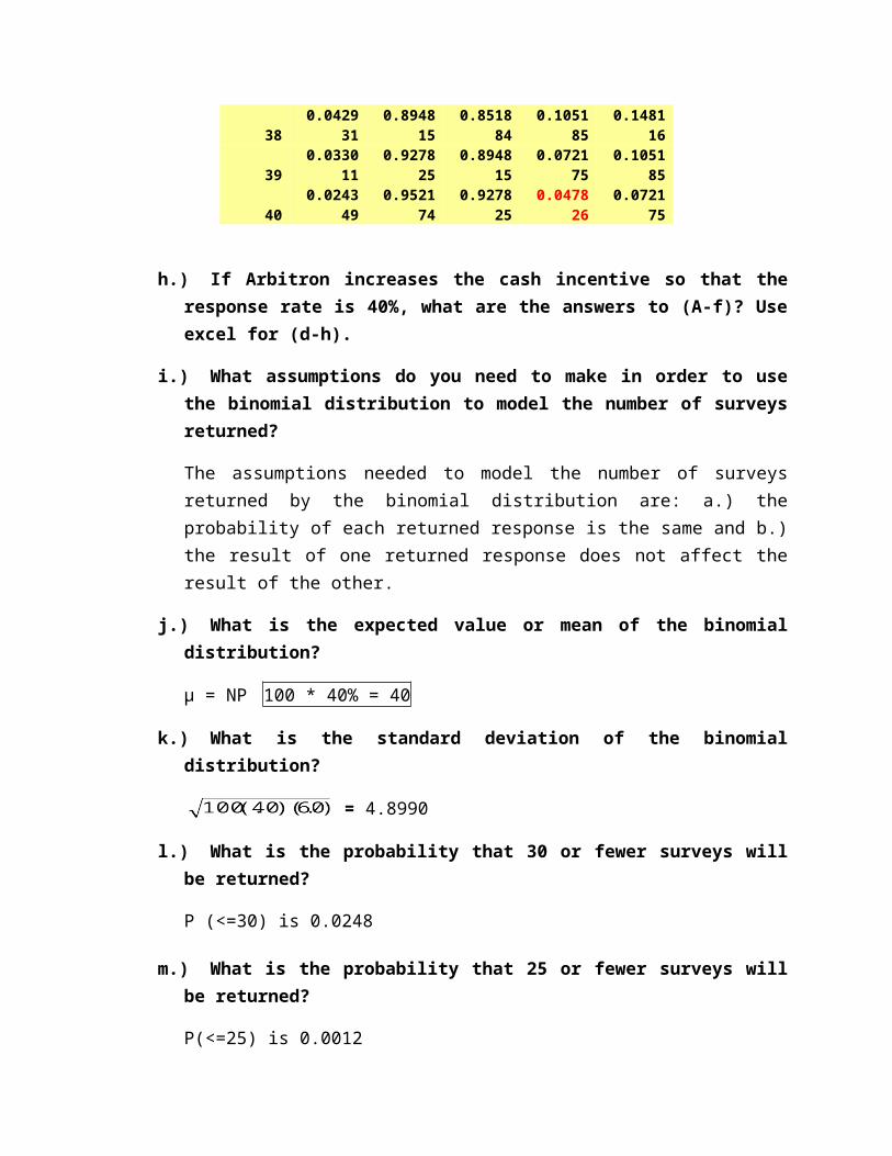
h.) If Arbitron increases the cash incentive so that the response rate is 40%, what are the answers to (A-f)? Use excel for (d-h).
i.) What assumptions do you need to make in order to use the binomial distribution to model the number of surveys returned?
The assumptions needed to model the number of surveys returned by the binomial distribution are: a.) the probability of each returned response is the same and b.) the result of one returned response does not affect the result of the other.
j.) What is the expected value or mean of the binomial distribution?
µ = NP 100 * 40% = 40
k.) What is the standard deviation of the binomial distribution?
= 4.8990
l.) What is the probability that 30 or fewer surveys will be returned?
P (<=30) is 0.0248
m.) What is the probability that 25 or fewer surveys will be returned?
P(<=25) is 0.0012
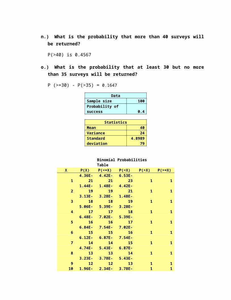
n.) What is the probability that more than 40 surveys will be returned?
P(>40) is 0.4567
o.) What is the probability that at least 30 but no more than 35 surveys will be returned?
P (>=30) - P(>35) = 0.1647
DataSample size 100Probability of success 0.4
StatisticsMean 40Variance 24Standard deviation 4.898979
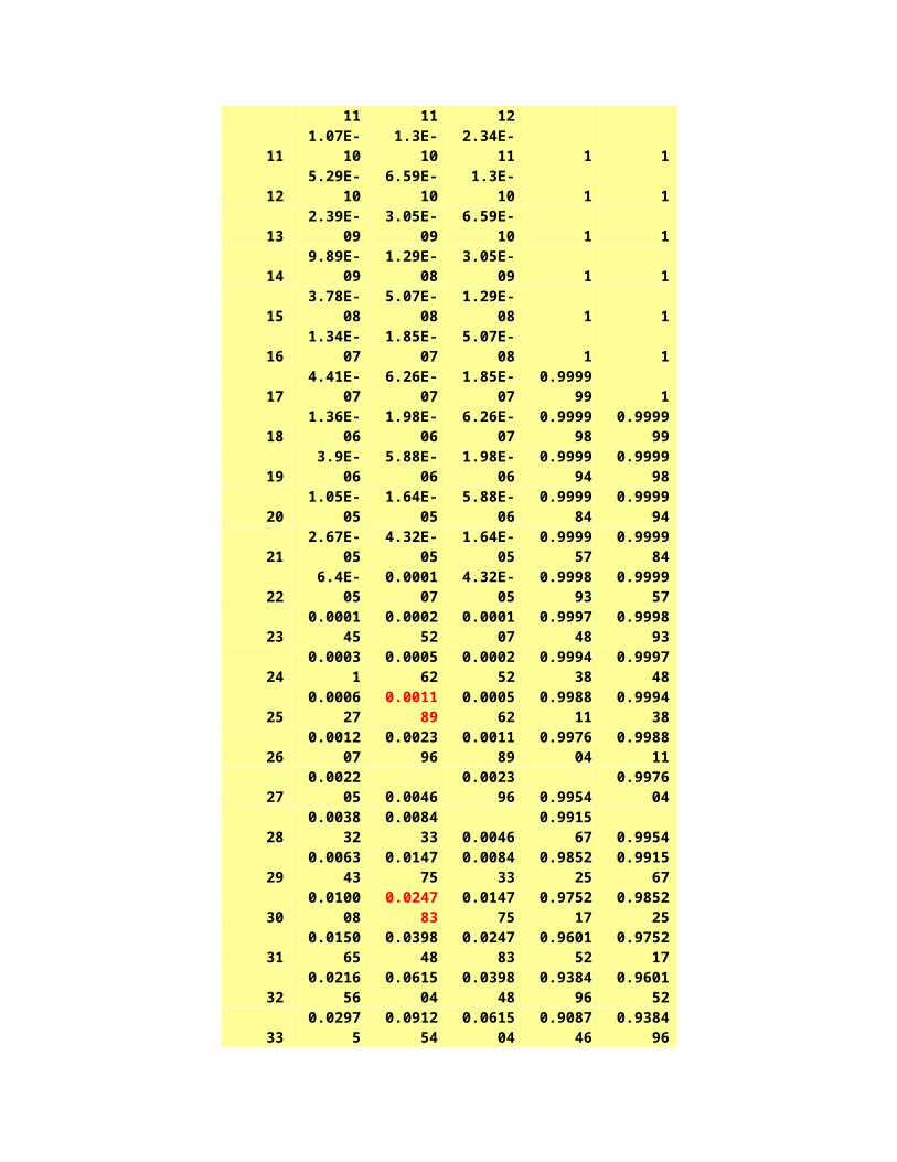
Binomial Probabilities TableX P(X) P(<=X) P(<X) P(>X) P(>=X)
1 4.36E-21 4.42E-21 6.53E-23 1 12 1.44E-19 1.48E-19 4.42E-21 1 13 3.13E-18 3.28E-18 1.48E-19 1 14 5.06E-17 5.39E-17 3.28E-18 1 15 6.48E-16 7.02E-16 5.39E-17 1 16 6.84E-15 7.54E-15 7.02E-16 1 17 6.12E-14 6.87E-14 7.54E-15 1 18 4.74E-13 5.43E-13 6.87E-14 1 19 3.23E-12 3.78E-12 5.43E-13 1 1
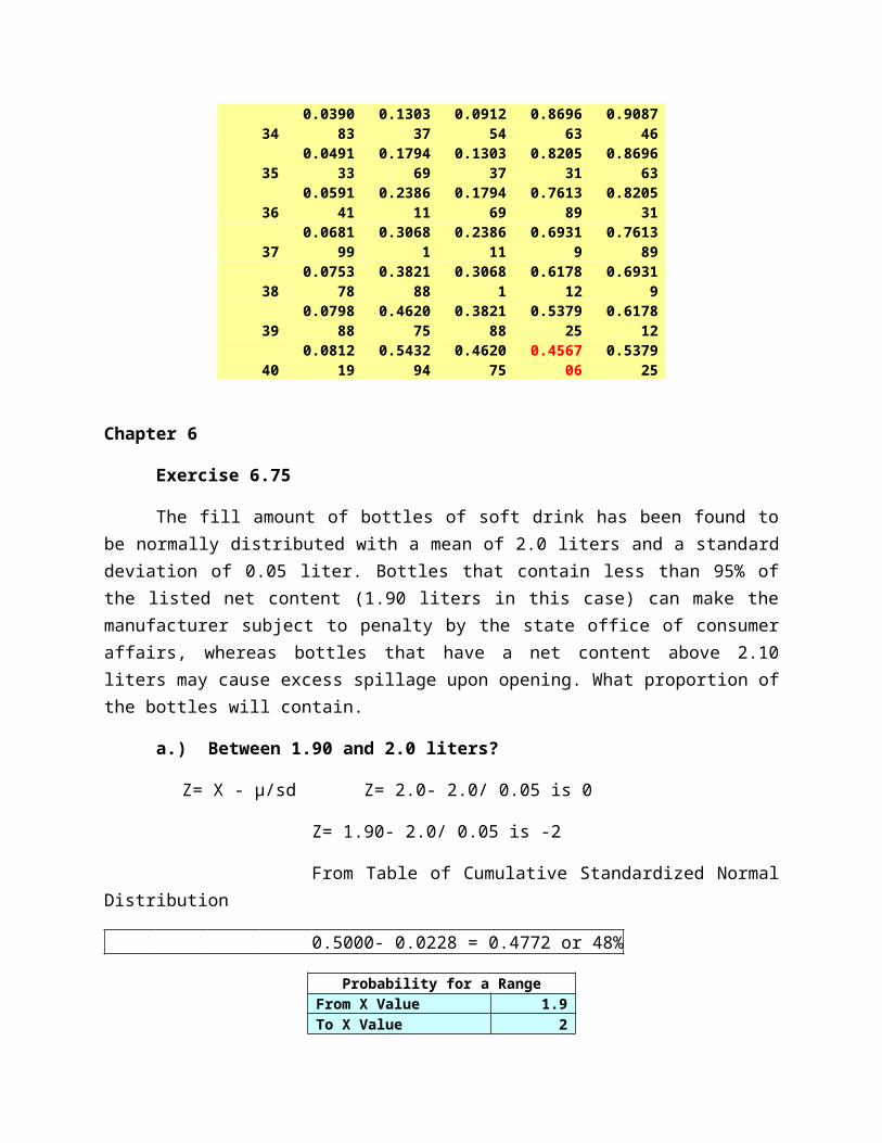
10 1.96E-11 2.34E-11 3.78E-12 1 111 1.07E-10 1.3E-10 2.34E-11 1 112 5.29E-10 6.59E-10 1.3E-10 1 113 2.39E-09 3.05E-09 6.59E-10 1 114 9.89E-09 1.29E-08 3.05E-09 1 115 3.78E-08 5.07E-08 1.29E-08 1 116 1.34E-07 1.85E-07 5.07E-08 1 117 4.41E-07 6.26E-07 1.85E-07 0.999999 118 1.36E-06 1.98E-06 6.26E-07 0.999998 0.99999919 3.9E-06 5.88E-06 1.98E-06 0.999994 0.99999820 1.05E-05 1.64E-05 5.88E-06 0.999984 0.99999421 2.67E-05 4.32E-05 1.64E-05 0.999957 0.99998422 6.4E-05 0.000107 4.32E-05 0.999893 0.99995723 0.000145 0.000252 0.000107 0.999748 0.99989324 0.00031 0.000562 0.000252 0.999438 0.99974825 0.000627 0.001189 0.000562 0.998811 0.99943826 0.001207 0.002396 0.001189 0.997604 0.99881127 0.002205 0.0046 0.002396 0.9954 0.99760428 0.003832 0.008433 0.0046 0.991567 0.995429 0.006343 0.014775 0.008433 0.985225 0.99156730 0.010008 0.024783 0.014775 0.975217 0.98522531 0.015065 0.039848 0.024783 0.960152 0.97521732 0.021656 0.061504 0.039848 0.938496 0.960152
33 0.02975 0.091254 0.061504 0.908746 0.93849634 0.039083 0.130337 0.091254 0.869663 0.90874635 0.049133 0.179469 0.130337 0.820531 0.86966336 0.059141 0.238611 0.179469 0.761389 0.82053137 0.068199 0.30681 0.238611 0.69319 0.76138938 0.075378 0.382188 0.30681 0.617812 0.6931939 0.079888 0.462075 0.382188 0.537925 0.61781240 0.081219 0.543294 0.462075 0.456706 0.537925
Chapter 6
Exercise 6.75
The fill amount of bottles of soft drink has been found to be normally distributed with a mean of 2.0 liters and a standard deviation of 0.05 liter. Bottles that contain less than 95% of the listed net content (1.90 liters in this case) can make the manufacturer subject to penalty by the state office of consumer affairs, whereas bottles that have a net content above 2.10 liters may cause excess spillage upon opening. What proportion of the bottles will contain.
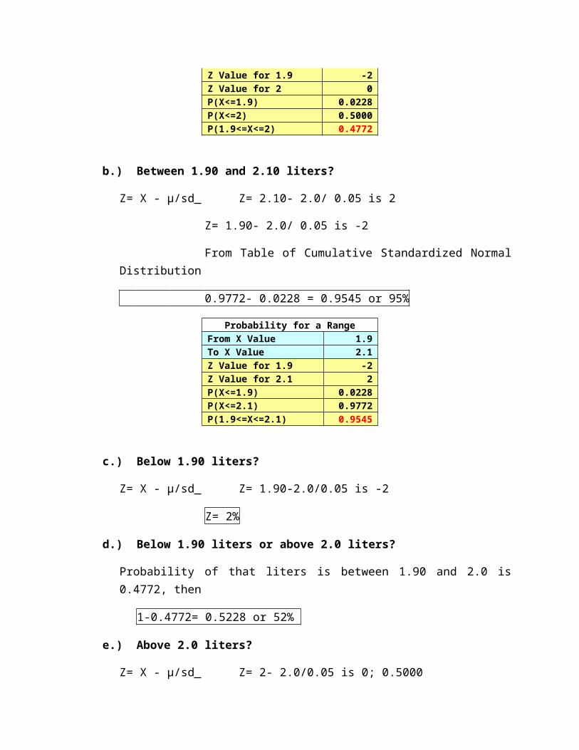
a.) Between 1.90 and 2.0 liters?
Z= X - µ/sd Z= 2.0- 2.0/ 0.05 is 0
Z= 1.90- 2.0/ 0.05 is -2
From Table of Cumulative Standardized Normal Distribution
0.5000- 0.0228 = 0.4772 or 48%
Probability for a RangeFrom X Value 1.9To X Value 2Z Value for 1.9 -2Z Value for 2 0P(X<=1.9) 0.0228P(X<=2) 0.5000P(1.9<=X<=2) 0.4772
b.) Between 1.90 and 2.10 liters?
Z= X - µ/sd Z= 2.10- 2.0/ 0.05 is 2
Z= 1.90- 2.0/ 0.05 is -2
From Table of Cumulative Standardized Normal Distribution
0.9772- 0.0228 = 0.9545 or 95%
Probability for a RangeFrom X Value 1.9To X Value 2.1Z Value for 1.9 -2Z Value for 2.1 2P(X<=1.9) 0.0228P(X<=2.1) 0.9772P(1.9<=X<=2.1) 0.9545
c.) Below 1.90 liters?
Z= X - µ/sd Z= 1.90-2.0/0.05 is -2
Z= 2%
d.) Below 1.90 liters or above 2.0 liters?
Probability of that liters is between 1.90 and 2.0 is 0.4772, then
1-0.4772= 0.5228 or 52%
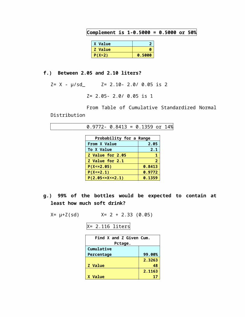
e.) Above 2.0 liters?
Z= X - µ/sd Z= 2- 2.0/0.05 is 0; 0.5000
Complement is 1-0.5000 = 0.5000 or 50%
X Value 2Z Value 0P(X>2) 0.5000
f.) Between 2.05 and 2.10 liters?
Z= X - µ/sd Z= 2.10- 2.0/ 0.05 is 2
Z= 2.05- 2.0/ 0.05 is 1
From Table of Cumulative Standardized Normal Distribution
0.9772- 0.8413 = 0.1359 or 14%
Probability for a RangeFrom X Value 2.05To X Value 2.1
Z Value for 2.05 1Z Value for 2.1 2P(X<=2.05) 0.8413P(X<=2.1) 0.9772P(2.05<=X<=2.1) 0.1359
g.) 99% of the bottles would be expected to contain at least how much soft drink?
X= µ+Z(sd) X= 2 + 2.33 (0.05)
X= 2.116 liters
Find X and Z Given Cum. Pctage.Cumulative Percentage 99.00%Z Value 2.326348X Value 2.116317
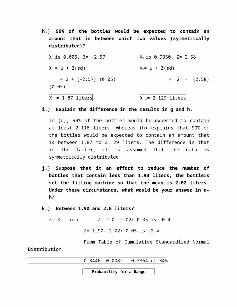
h.) 99% of the bottles would be expected to contain an amount that is between which two values (symmetrically distributed)?
XL is 0.005, Z= -2.57 XU is 0.9950, Z= 2.58
XL = µ + Z(sd) XU= µ + Z(sd)
= 2 + (-2.57) (0.05) = 2 + (2.58) (0.05)
X L= 1.87 liters X u= 2.129 liters
i.) Explain the difference in the results in g and h.
In (g), 99% of the bottles would be expected to contain at least 2.116 liters, whereas (h) explains that 99% of the bottles would be expected to contain an amount that is between 1.87 to 2.129 liters. The difference is that in the latter, it is assumed that the data is symmetrically distributed.
j.) Suppose that it an effort to reduce the number of bottles that contain less than 1.90 liters, the bottlers set the filling machine so that the mean is 2.02 liters. Under these circumstance, what would be your answer in a- h?
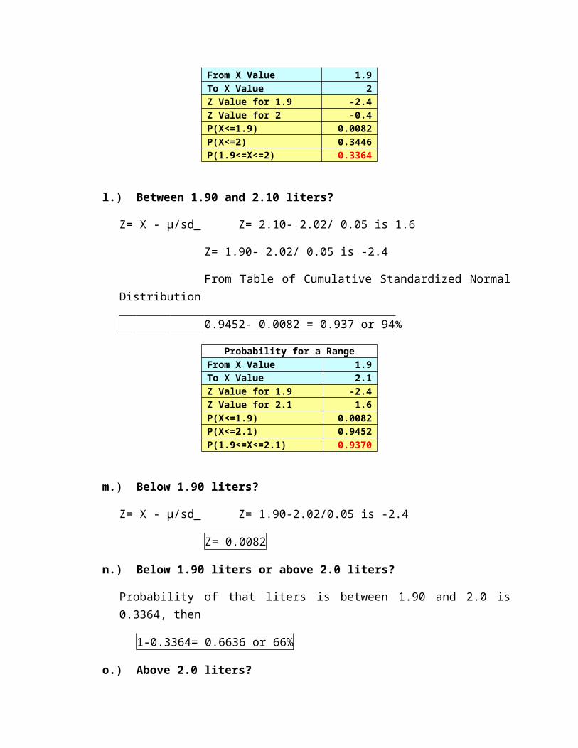
k.) Between 1.90 and 2.0 liters?
Z= X - µ/sd Z= 2.0- 2.02/ 0.05 is -0.4
Z= 1.90- 2.02/ 0.05 is -2.4
From Table of Cumulative Standardized Normal Distribution
0.3446- 0.0082 = 0.3364 or 34%
Probability for a RangeFrom X Value 1.9To X Value 2Z Value for 1.9 -2.4Z Value for 2 -0.4P(X<=1.9) 0.0082P(X<=2) 0.3446P(1.9<=X<=2) 0.3364
l.) Between 1.90 and 2.10 liters?
Z= X - µ/sd Z= 2.10- 2.02/ 0.05 is 1.6
Z= 1.90- 2.02/ 0.05 is -2.4
From Table of Cumulative Standardized Normal Distribution
0.9452- 0.0082 = 0.937 or 94%
Probability for a RangeFrom X Value 1.9To X Value 2.1Z Value for 1.9 -2.4Z Value for 2.1 1.6P(X<=1.9) 0.0082P(X<=2.1) 0.9452P(1.9<=X<=2.1) 0.9370
m.) Below 1.90 liters?
Z= X - µ/sd Z= 1.90-2.02/0.05 is -2.4
Z= 0.0082
n.) Below 1.90 liters or above 2.0 liters?
Probability of that liters is between 1.90 and 2.0 is 0.3364, then
1-0.3364= 0.6636 or 66%
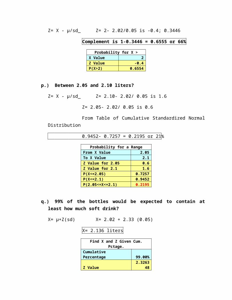
o.) Above 2.0 liters?
Z= X - µ/sd Z= 2- 2.02/0.05 is -0.4; 0.3446
Complement is 1-0.3446 = 0.6555 or 66%
Probability for X >X Value 2Z Value -0.4P(X>2) 0.6554
p.) Between 2.05 and 2.10 liters?
Z= X - µ/sd Z= 2.10- 2.02/ 0.05 is 1.6
Z= 2.05- 2.02/ 0.05 is 0.6
From Table of Cumulative Standardized Normal Distribution
0.9452- 0.7257 = 0.2195 or 21%
Probability for a RangeFrom X Value 2.05To X Value 2.1Z Value for 2.05 0.6Z Value for 2.1 1.6P(X<=2.05) 0.7257P(X<=2.1) 0.9452P(2.05<=X<=2.1) 0.2195
q.) 99% of the bottles would be expected to contain at least how much soft drink?
X= µ+Z(sd) X= 2.02 + 2.33 (0.05)
X= 2.136 liters
Find X and Z Given Cum. Pctage.Cumulative Percentage 99.00%Z Value 2.326348X Value 2.136317
r.) 99% of the bottles would be expected to contain an amount that is between which two values (symmetrically distributed)?
XL is 0.005, Z= -2.57 XU is 0.9950, Z= 2.58
XL = µ + Z(sd) XU= µ + Z(sd)
= 2.02 + (-2.57) (0.05) = 2.02 + (2.58) (0.05)
X L= 1.8915 liters X u= 2.149 liters
s.) Explain the difference in the results in g and h.
In (g), 99% of the bottles would be expected to contain at least 2.136 liters, whereas (h) explains that 99% of the bottles would be expected to contain an amount that is between 1.8915 to 2.149 liters. The difference is that in the latter, it is assumed that the data is symmetrically distributed.
If a random sample of 25 bottles is selected, what is the probability that the sample mean will be
t.) Between 1.99 and 2.0 liters?
Z = X – μ = 2.0- 2.0 σ/√n .05/√25 = 0
Z = X – μ = 1.99- 2.0 σ/√n .05/√25
= -0.001 0.01= -.1
From Table of Cumulative Standardized Normal Distribution
0.5000- 0.4602 = 0.398 or 39.8%
u.) Between 1.99 and 2.01 liters?
Z = X – μ = 2.01- 2.0 σ/√n .05/√25 = 1
Z = X – μ = 1.99- 2.0 σ/√n .05/√25
= -0.001 0.01= -.1
From Table of Cumulative Standardized Normal Distribution
0.8413- 0.4602 = 0.3811 or 38.11%
v.) Below 1.98 liters?
Z = X – μ = 1.98- 2.0 σ/√n .05/√25
= -0.02 0.01
= -2; or 0.0228 or 2.28% of the sample size 25 would be expected to have means below 1.98L
w.) Below 1.98 liters or above 2.02 liters?
Z = X – μ = 1.98- 2.0 σ/√n .05/√25
= -0.02 0.01= -2 or 0.0228 or 2.28%
Z = X – μ = 2.02- 2.0 σ/√n .05/√25
= 0.02 0.01= 2; or 0.9772 or 97.72%
Complement is 1- 0.9772 = 0.0228
0.0228 + 0.9772 = 1
x.) Above 2.01 liters?
Z = X – μ = 2.01- 2.0 σ/√n .05/√25
= 0.01 0.01= 1; or 0.8413 or 84.13%
Complement is 1- 0.8413 = 0.1587 or 15.87% is above 2.01 liters
y.) Between 2.01 and 2.03 liters?
Z = X – μ = 2.01- 2.0 σ/√n .05/√25 = 1
Z = X – μ = 2.03- 2.0 σ/√n .05/√25
= -0.03 0.01= -3
From Table of Cumulative Standardized Normal Distribution
0.8413- 0.00135 = 0.83995 or 83.99%
z.) 99% of the sample means would be expected to contain at least how much soft drink?
2.023263
Find X and Z Given Cum. Pctage.
Cumulative Percentage 99.00%
Z Value 2.326348
X Value 2.023263
aa.) 99% of the sample means would be expected to contain an amount that is between which two values (symmetrically distributed around the mean?)
XL is 0.05, Z= -2.58 XU is 0.995, Z= +2.58
XL = µ + Z(.40/ ) XU= µ + Z(.40/ )
= 2.0 + (-2.58) (0.08) = 4.70 + (+2.58) (0.08)
X L= 1.7936 liters X u= 2.2064 ounces
bb.) Explain the difference in results in q and r.
In (q), 99% of the bottles would be expected to contain at least 2.0232 liters, whereas (r) explains that 99% of the bottles would be expected to contain an amount that is between 1.7936 to 2.2064 liters. The difference is that in the latter, it is assumed that the data is symmetrically distributed.
Exercise 6.76
An orange producer buys all his oranges from a large orange grove. The amount of juice squeezed from each of these oranges is approximately normally distributed with a mean of 4.70 ounces and a standard deviation of 0.40 ounce.
a.) What is the probability that a randomly selected orange will contain between 4.70 and 5.00 ounces?
Z= X - µ/sd Z= 5.00- 4.70/ 0.40 is 0.75
Z= 4.70- 4.70/ 0.40 is 0
From Table of Cumulative Standardized Normal Distribution
0.7734- 0.5000 = 0.2734
Probability for a RangeFrom X Value 4.7To X Value 5Z Value for 4.7 0Z Value for 5 0.75P(X<=4.7) 0.5000P(X<=5) 0.7734P(4.7<=X<=5) 0.2734
b.) What is the probability that a randomly selected orange will contain between 5.00 and 5.50 ounces?
Z= X - µ/sd Z= 5.50- 4.70/ 0.40 is 2
Z= 5.00- 4.70/ 0.40 is 0.75
From Table of Cumulative Standardized Normal Distribution
0.9772- 0.7734 = 0.2038
Probability for a RangeFrom X Value 5To X Value 5.5Z Value for 5 0.75Z Value for 5.5 2P(X<=5) 0.7734P(X<=5.5) 0.9772P(5<=X<=5.5) 0.2039
c.) 77% of the oranges will contain at least how many ounces of juice?
X= µ+Z(sd) X= 4.70 + 0.74 (0.40)
X = 4.996 ounces
Find X and Z Given Cum. Pctage.Cumulative Percentage 77.00%Z Value 0.738846849X Value 4.99553874
d.) Between what two values (in ounces) symmetrically distributed around the population mean will 80 % of the oranges fall?
XL is 0.10, Z= - 1.26 XU is 0.90, Z= +1.26
XL = µ + Z(sd) XU= µ + Z(sd)
= 4.70 + (-1.26) (0.40) = 4.70 + (+1.26) (0.40)
X L= 4.19 ounces X u= 5.212 ounces
Suppose that a sample of 25 oranges is selected:
e.) What is the probability that the sample mean will be at least 4.60 ounces?
_ Z = X – μ = 4.70- 4.60
σ/√n .4/√25
= 0.1 0.08
= 1.25; or 0.894489.44% of all the possible samples of size 25 have a sample mean of at least 4.60 ounces.
f.) Between what two values symmetrically distributed around the population mean will 70% of the sample mean fall?
XL is 0.15, Z= -1.04 XU is 0.85, Z= +1.04
XL = µ + Z(.40/ ) XU= µ + Z(.40/ )
= 4.70 + (-1.04) (0.08) = 4.70 + (+1.04) (0.08)
X L= 4.6168 ounces X u= 4.7832 ounces
g.) 77% of the sample means will be above what value?
X= µ+Z(sd) X= 4.70 + -0.74 (0.08)
X = 4.6408 ounces