Probability density function of the intensity of a laser ...Probability density function of the intensity of a laser beam propagating ... Vol. 2 of Methods of Modern Mathematical Physics

Probability density function of the intensity of a laser beam propagating

in the maritime environment Olga Korotkova,1,* Svetlana Avramov-Zamurovic,2 Reza Malek-Madani,3 and

Charles Nelson4 1Department of Physics, University of Miami, 1320 Campo Sano Dr., Coral Gables, FL 33146, USA

2Weapons and Systems Engineering Department of Mathematics, US Naval Academy, 105 Maryland Avenue, Annapolis, MD 21402, USA

3Department of Mathematics, US Naval Academy, 589 McNair Rd, Stop 10M, Annapolis, MD 21402, USA 4Computer and Electrical Engineering Department, US Naval Academy, 105 Maryland Avenue, Annapolis,

MD 21402, USA *[email protected]

Abstract: A number of field experiments measuring the fluctuating intensity of a laser beam propagating along horizontal paths in the maritime environment is performed over sub-kilometer distances at the United States Naval Academy. Both above the ground and over the water links are explored. Two different detection schemes, one photographing the beam on a white board, and the other capturing the beam directly using a ccd sensor, gave consistent results. The probability density function (pdf) of the fluctuating intensity is reconstructed with the help of two theoretical models: the Gamma-Gamma and the Gamma-Laguerre, and compared with the intensity’s histograms. It is found that the on-ground experimental results are in good agreement with theoretical predictions. The results obtained above the water paths lead to appreciable discrepancies, especially in the case of the Gamma-Gamma model. These discrepancies are attributed to the presence of the various scatterers along the path of the beam, such as water droplets, aerosols and other airborne particles. Our paper’s main contribution is providing a methodology for computing the pdf function of the laser beam intensity in the maritime environment using field measurements. ©2011 Optical Society of America OCIS codes: (010.1300) Atmospheric propagation; (010.3310) Laser beam transmission; (010.7060) Turbulence.

References and links 1. A. Ishimaru, Electromagnetic Wave Propagation, Radiation, and Scattering (Prentice Hall, 1996). 2. V. I. Tatarskii, Wave Propagation in a Turbulent Medium (McGraw-Hill, New York, 1961; reproduced by

Dover, New York, 1967). 3. S. F. Clifford, “The classical theory of wave propagation in a turbulent medium,” in Laser Beam Propagation in

the Atmosphere, J. Strohbehn, ed.(Springer, New York, 1978). 4. R. L. Fante, “Wave propagation in random media: a system approach,” Progress in Optics Vol 22, E. Wolf, ed.

(Elsevier, Amsterdam, 1985). 5. L. C. Andrews and R. L. Phillips, Laser Beam Propagation in Random Media, 2nd ed. (SPIE Press, Bellingham,

Washington, 2005). 6. L. C. Andrews, R. L. Phillips, and C. Y. Hopen, Electromagnetic Beam Scintillation with Applications (SPIE

Press, Bellingham, Washington, 2001). 7. D. Wheelon, Electromagnetic Scintillation II Weak Scattering (Cambridge University Press, 2003) 8. S. Chandrasekhar, Radiative Transfer (Dover, 1960). 9. M. I. Mishchenko and L. D. Travis, Scattering, Absorption, and Emission of Light by Small Particles (Cambridge

University Press, 2002). 10. M. P. J. L. Chang, C. O. Font, G. C. Gilbreath, and E. Oh, “Humidity’s influence on visible region refractive

index structure parameter Cn2.,” Appl. Opt. 46(13), 2453–2459 (2007).

11. R. J. Hill, “Spectra of fluctuations in refractivity, temperature, humidity, and the temperature-humidity cospectrum in the inertial and dissipation ranges,” Radio Sci. 13(6), 953–961 (1978).

#149212 - $15.00 USD Received 14 Jun 2011; revised 22 Aug 2011; accepted 25 Aug 2011; published 3 Oct 2011(C) 2011 OSA 10 October 2011 / Vol. 19, No. 21 / OPTICS EXPRESS 20322

12. C. A. Friehe, J. C. La Rue, F. H. Champagne, C. H. Gibson, and G. F. Dreyer, “Effects of temperature and humidity fluctuations on the optical refractive index in the marine boundary layer,” J. Opt. Soc. Am. 65(12), 1502–1511 (1975).

13. R. Weiss-Wrana, “Turbulence statistics in littoral area,” Proc. SPIE 6364, 63640F, 63640F-12 (2006). 14. J. Grayshan, F. S. Vetelino, and C. Y. Young, “A marine atmospheric spectrum for laser propagation,” Waves

Random Complex Media 18(1), 173–184 (2008). 15. K. J. Mayer and C. Y. Young, “Effect of atmospheric spectrum models on scintillation in moderate turbulence,”

J. Mod. Opt. 55(7), 1101–1117 (2008). 16. M. Reed and B. Simon, Fourier Analysis, Self-Adjointness, Vol. 2 of Methods of Modern Mathematical Physics

(Academic, 1975), p. 341. 17. J. A. Shehat and J. D. Tamarkin, The Problem of Moments (American Mathematical Society, New York, 1943). 18. W. Feller, An Introduction to Probability Theory and its Applications (Wiley, 1971), Vol. II. 19. M. A. Al-Habash, L. C. Andrews, and R. L. Phillips, “Mathematical model for the irradiance probability density

function of a laser beam propagating through turbulent media,” Opt. Eng. 40(8), 1554–1562 (2001). 20. R. Barakat, “First-order intensity and log-intensity probability density functions of light scattered by the turbulent

atmosphere in terms of lower-order moments,” J. Opt. Soc. Am. 16(9), 2269–2274 (1999).

1. Introduction

In dealing with random optical fields that interact with natural environments, the knowledge of the probability density functions of their intensity and phase are of utmost importance [1–3]. The majority of the theories describing these statistics have been developed either for light scattered from random collections of particles or for propagation in media where the refractive index changes continuously, but in a random manner. In particular, considerable amount of effort has been devoted to understanding how optical signals respond to perturbations due to the turbulence in the medium [4–7]. The crucial aspect of this research is to account for the complex interference effects that occur at every stage when the beam interacts with the medium. A good example of a medium where interference effects have been studied extensively is the clear-air turbulent atmosphere, i.e. the one in which aerosols, water droplets, dust and other particles are absent. An alternative approach to light-matter interactions in which the interference phenomenon is neglected, is radiative transfer [8]. This method is capable of predicting the characteristics of power transmitted through an absorptive, multiple scattering medium [9] while neglecting the interference phenomena.

A medium that involves both clear air optical turbulence and particle absorption/ scattering, is the atmosphere in the maritime environment. A large volume of water creates a situation where water droplets, bio-particles and various types of aerosols are present in abundance [10]. Maritime atmospheric environment has been not been studied extensively from the perspective of optical characterization [11–13]. A significant contribution is the recent development of maritime spatial power spectrum [14,15]. This research clearly shows that optical turbulence has distinctive features in the maritime atmosphere, compared to the above the ground atmosphere, such as an increased characteristic bump at high spatial frequencies.

The probability density function of any continuous random variable is a function whose integral over an interval gives the probability that the random variable attains a certain value in that interval. There are two traditional approaches of computing the pdf of a random variable: one is based on fitting data to a prescribed parametric function and the other one relies on a physical model of the phenomenon of interest. In the first category, the classical method is the method of moments, known as the Hausdorff moment problem [16–18]. Although the method of moments provides complete knowledge of phenomenon when infinitely many moments are known, its implementation is not often practical due to measurement uncertainties and computational limitations. Typically, available data is discrete as well as time and space limited. Physics based models, on the other hand, are generally statistically robust, but they are obtained using a number of assumptions that may lead to limitations of their scope of applicability. The third approach, developed recently, is based on the hybrid of the two methods, where a pdf is constructed in terms of physics-based basis functions and a weighted set of moments.

In our study we use two hybrid methods, one called the Gamma-Gamma method, outlined in [19], and the other Gamma-Laguerre, described in [20]. The Gamma-Gamma method is


predominantly physics based and is known to best represent propagation of a Gaussian beam along its optical axis. Its derivation relies on detailed statistical knowledge of the atmosphere, and its implementation uses only a single statistical parameter of the beam, namely the variance of the fluctuating beam intensities. The Gamma-Laguerre method, on the other hand, has the advantage of including scattering effects on the beam. In practice its implementation uses up to 5 or more weighted moments.

From an application point of view knowledge of the probability density function of the fluctuating beam intensities is crucial for solving inverse problems for determining the statistics of a medium. It is well-known that the tails of a pdf influence the fade statistics of a signal encoded in a beam (the so called Bit Error Rates in a communication channel) [5,6]. Our paper’s main goal is to provide a methodology for computing the pdf function of the laser beam intensity in the maritime environment using field measurements.

The paper is organized as follows. In section 2 the experimental setup and atmospheric conditions are described for the two campaigns. In Section 3 we review the two pdf analytical models of the Gaussian beam intensity. Section 4 deals with description of the data post-processing. In Section 5, the results of two campaigns are presented and compared.

2. Experiment

Several experiments to collect data on laser beam propagation were conducted at the United States Naval Academy, one set during June 2010 and anther set during March 2011. The source was a low power (2 mW) red He-Ne laser with an expander positioned on a tripod, generating a one centimeter wide Gaussian laser beam. This source proved to be reliably detected at distances around 500 m. For experiments carried out in June 2010 the fluctuating intensity was reflected off of a white board and captured by a video camera. For the March 2011 experiments, the beam intensity was recorded directly by a monochromatic charge-coupled device (ccd) imaging sensor. To minimize the background light a red light notch filter was used. Also, a set of neutral density attenuating filters were used to adjust the span of recorded light intensities within the linear sensitivity range. The sensitivity of the ccd sensor is eight bits, providing 256 possible levels of intensity. The sensing area is 7.6 mm (horizontal) × 6.2 mm (vertical) with pixel size of 4.65 μm. The pixel size is small compared to the coherence radius which is calculated to be around the order of 1 cm. The sensing area is large enough to allow observation of the central part of the beam. This is important because we are interested in the probability density function of light intensity at a single point at the center of the beam as required by Gamma-Gamma model assumptions. Several three minutes video segments were recorded and converted to single pictures (frames) for processing purposes. The simplicity of the experimental set-up offers measurements of beam intensity with minimal effects from optical components in the path of the laser beam. All of the experiments were conducted in dry, partially sunny weather, at mid-day.

Equivalent to the spatial limitations on the sampling rate defined by the coherence radius, temporal limitations are influenced by the wind velocity. In some of the field experiments there was no measured wind. In the laboratory set up we measured the laser propagation in a motionless tunnel with the heat screen and did not observe any feature different compared to the ones from outdoors (with some wind blowing).

Figure 1(a) shows the experimental run on June 15, 2010 over a 400 m link on the grassy football field (Forrest Sherman Field). Figure 1(b) shows a similar experiment done on June 18 across College Creek. The weather conditions for the two June experiments are given in Tables 1 and 2, respectively. The data is collected from the Hospital Point National Weather station located on Sherman Field and the tables present conditions during the test run.

Figure 2 shows the experiments run on March 15, 2011 over 300 m links (a) on the Forrest Sherman field and (b) across the College Creek. The weather conditions for these two tests collected from Hospital Point National Weather Station located on the Sherman Field are given in the Table 3.


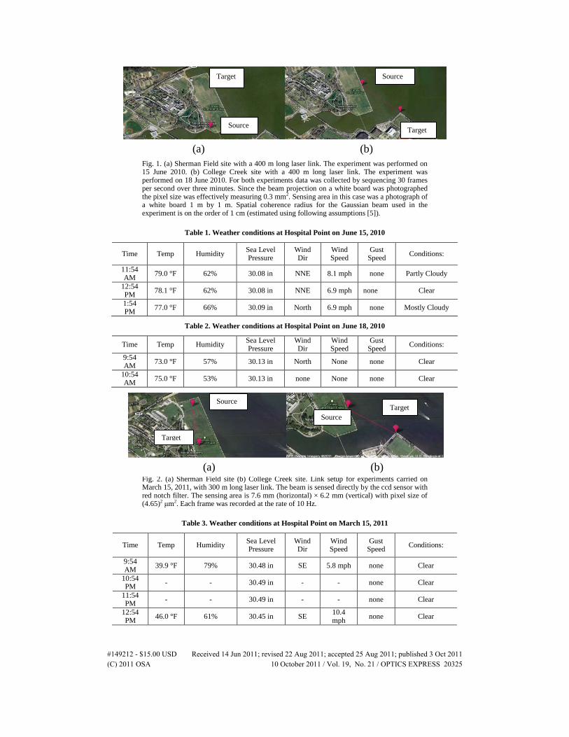
Fig. 1. (a) Sherman Field site with a 400 m long laser link. The experiment was performed on 15 June 2010. (b) College Creek site with a 400 m long laser link. The experiment was performed on 18 June 2010. For both experiments data was collected by sequencing 30 frames per second over three minutes. Since the beam projection on a white board was photographed the pixel size was effectively measuring 0.3 mm2. Sensing area in this case was a photograph of a white board 1 m by 1 m. Spatial coherence radius for the Gaussian beam used in the experiment is on the order of 1 cm (estimated using following assumptions [5]).

Table 1. Weather conditions at Hospital Point on June 15, 2010

Time Temp Humidity Sea Level Pressure

Wind Dir

Wind Speed

Gust Speed Conditions:

11:54 AM 79.0 °F 62% 30.08 in NNE 8.1 mph none Partly Cloudy

12:54 PM 78.1 °F 62% 30.08 in NNE 6.9 mph none Clear

1:54 PM 77.0 °F 66% 30.09 in North 6.9 mph none Mostly Cloudy

Table 2. Weather conditions at Hospital Point on June 18, 2010


Wind Dir

Wind Speed


9:54 AM 73.0 °F 57% 30.13 in North None none Clear

10:54 AM 75.0 °F 53% 30.13 in none None none Clear

Fig. 2. (a) Sherman Field site (b) College Creek site. Link setup for experiments carried on March 15, 2011, with 300 m long laser link. The beam is sensed directly by the ccd sensor with red notch filter. The sensing area is 7.6 mm (horizontal) × 6.2 mm (vertical) with pixel size of (4.65)2 μm2. Each frame was recorded at the rate of 10 Hz.

Table 3. Weather conditions at Hospital Point on March 15, 2011


Wind Dir

Wind Speed


9:54 AM 39.9 °F 79% 30.48 in SE 5.8 mph none Clear

10:54 PM - - 30.49 in - - none Clear

11:54 PM - - 30.49 in - - none Clear

12:54 PM 46.0 °F 61% 30.45 in SE 10.4

mph none Clear

Target

Source

Source

Target

(a) (b)

Target

Target Source

Source

(a) (b)


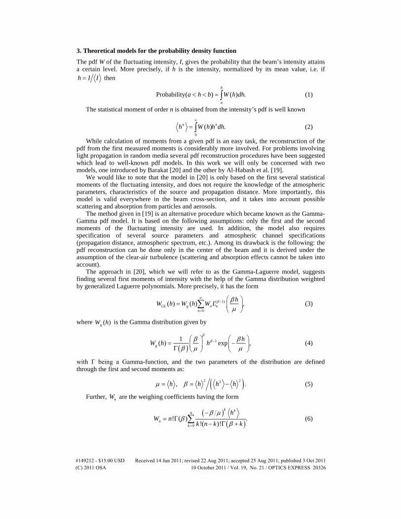
3. Theoretical models for the probability density function

The pdf W of the fluctuating intensity, I, gives the probability that the beam’s intensity attains a certain level. More precisely, if h is the intensity, normalized by its mean value, i.e. if

IIh = then

Probability( ) ( ) .b

a

a h b W h dh< < = ∫ (1)

The statistical moment of order n is obtained from the intensity’s pdf is well known

0

( ) .n nh W h h dh∞

= ∫ (2)

While calculation of moments from a given pdf is an easy task, the reconstruction of the pdf from the first measured moments is considerably more involved. For problems involving light propagation in random media several pdf reconstruction procedures have been suggested which lead to well-known pdf models. In this work we will only be concerned with two models, one introduced by Barakat [20] and the other by Al-Habash et al. [19].

We would like to note that the model in [20] is only based on the first several statistical moments of the fluctuating intensity, and does not require the knowledge of the atmospheric parameters, characteristics of the source and propagation distance. More importantly, this model is valid everywhere in the beam cross-section, and it takes into account possible scattering and absorption from particles and aerosols.

The method given in [19] is an alternative procedure which became known as the Gamma-Gamma pdf model. It is based on the following assumptions: only the first and the second moments of the fluctuating intensity are used. In addition, the model also requires specification of several source parameters and atmospheric channel specifications (propagation distance, atmospheric spectrum, etc.). Among its drawback is the following: the pdf reconstruction can be done only in the center of the beam and it is derived under the assumption of the clear-air turbulence (scattering and absorption effects cannot be taken into account).

The approach in [20], which we will refer to as the Gamma-Laguerre model, suggests finding several first moments of intensity with the help of the Gamma distribution weighted by generalized Laguerre polynomials. More precisely, it has the form

( 1)

0( ) ( ) ,GL g n n

n

hW h W h W L β βµ

∞−

=

=

∑ (3)

where ( )gW h is the Gamma distribution given by

( )

11( ) exp ,ghW h h

βββ β

β µ µ−

= − Γ (4)

with Г being a Gamma-function, and the two parameters of the distribution are defined through the first and second moments as:

( )2 22, .h h h hµ β= = − (5)

Further, nW are the weighing coefficients having the form

( )

( )0! ( ) .

!( )!

k kn

nk

hW n

k n k k

β µβ

β=

−= Γ

− Γ +∑ (6)


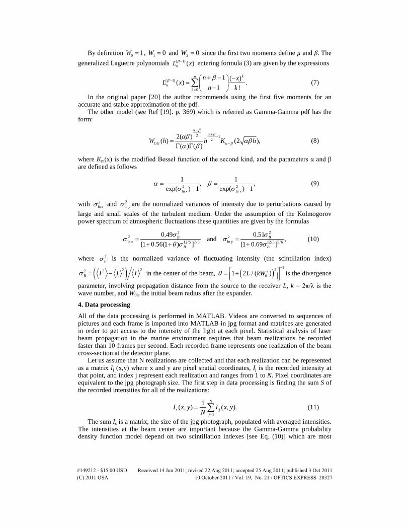
By definition 0 1W = , 1 0W = and 2 0W = since the first two moments define µ and β. The generalized Laguerre polynomials ( 1) ( )nL xβ − entering formula (3) are given by the expressions

( 1)

0

1 ( )( ) .1 !

kn

nk

n xL xn k

β β−

=

+ − −= − ∑ (7)

In the original paper [20] the author recommends using the first five moments for an accurate and stable approximation of the pdf.

The other model (see Ref [19]. p. 369) which is referred as Gamma-Gamma pdf has the form:

2 1

22( )( ) (2 ),( ) ( )GGW h h K h

α βα β

α βαβ αβα β

++

−

−=Γ Γ

(8)

where Km(x) is the modified Bessel function of the second kind, and the parameters α and β are defined as follows

2 2ln ln

1 1, ,exp( ) 1 exp( ) 1x y

α βσ σ

= =− −

(9)

with 2ln xσ and 2

ln yσ are the normalized variances of intensity due to perturbations caused by large and small scales of the turbulent medium. Under the assumption of the Kolmogorov power spectrum of atmospheric fluctuations these quantities are given by the formulas

2 2

2 2ln ln12/5 7/6 12/5 5/6

0.49 0.51and ,

[1 0.56(1 ) ] [1 0.69 ]B B

x yB B

σ σσ σ

θ σ σ= =

+ + + (10)

where 2Bσ is the normalized variance of fluctuating intensity (the scintillation index)

( )2 22 2B I I Iσ = − in the center of the beam, ( )

12201 2 / ( )L kWθ

− = +

is the divergence

parameter, involving propagation distance from the source to the receiver L, k = 2π/λ is the wave number, and W0is the initial beam radius after the expander.

4. Data processing

All of the data processing is performed in MATLAB. Videos are converted to sequences of pictures and each frame is imported into MATLAB in jpg format and matrices are generated in order to get access to the intensity of the light at each pixel. Statistical analysis of laser beam propagation in the marine environment requires that beam realizations be recorded faster than 10 frames per second. Each recorded frame represents one realization of the beam cross-section at the detector plane.

Let us assume that N realizations are collected and that each realization can be represented as a matrix Ij (x,y) where x and y are pixel spatial coordinates, Ij is the recorded intensity at that point, and index j represent each realization and ranges from 1 to N. Pixel coordinates are equivalent to the jpg photograph size. The first step in data processing is finding the sum S of the recorded intensities for all of the realizations:

1

1( , ) ( , ).N

s jj

I x y I x yN =

= ∑ (11)

The sum Is is a matrix, the size of the jpg photograph, populated with averaged intensities. The intensities at the beam center are important because the Gamma-Gamma probability density function model depend on two scintillation indexes [see Eq. (10)] which are most


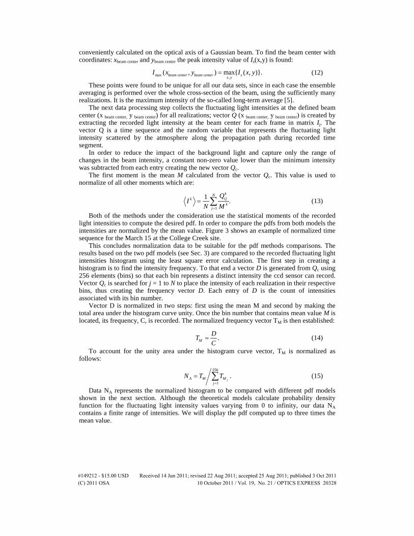
conveniently calculated on the optical axis of a Gaussian beam. To find the beam center with coordinates: xbeam center and ybeam center the peak intensity value of Is(x,y) is found:

max ,( , ) max{ ( , )}.beam center beam center sx y

I x y I x y= (12)

These points were found to be unique for all our data sets, since in each case the ensemble averaging is performed over the whole cross-section of the beam, using the sufficiently many realizations. It is the maximum intensity of the so-called long-term average [5].

The next data processing step collects the fluctuating light intensities at the defined beam center (x beam center, y beam center) for all realizations; vector Q (x beam center, y beam center) is created by extracting the recorded light intensity at the beam center for each frame in matrix Ij. The vector Q is a time sequence and the random variable that represents the fluctuating light intensity scattered by the atmosphere along the propagation path during recorded time segment.

In order to reduce the impact of the background light and capture only the range of changes in the beam intensity, a constant non-zero value lower than the minimum intensity was subtracted from each entry creating the new vector Qc.

The first moment is the mean M calculated from the vector Qc. This value is used to normalize of all other moments which are:

1

1 .kNcjkk

j

QI

N M=

= ∑ (13)

Both of the methods under the consideration use the statistical moments of the recorded light intensities to compute the desired pdf. In order to compare the pdfs from both models the intensities are normalized by the mean value. Figure 3 shows an example of normalized time sequence for the March 15 at the College Creek site.

This concludes normalization data to be suitable for the pdf methods comparisons. The results based on the two pdf models (see Sec. 3) are compared to the recorded fluctuating light intensities histogram using the least square error calculation. The first step in creating a histogram is to find the intensity frequency. To that end a vector D is generated from Qc using 256 elements (bins) so that each bin represents a distinct intensity the ccd sensor can record. Vector Qc is searched for j = 1 to N to place the intensity of each realization in their respective bins, thus creating the frequency vector D. Each entry of D is the count of intensities associated with its bin number.

Vector D is normalized in two steps: first using the mean M and second by making the total area under the histogram curve unity. Once the bin number that contains mean value M is located, its frequency, C, is recorded. The normalized frequency vector TM is then established:

.MDTC

= (14)

To account for the unity area under the histogram curve vector, TM is normalized as follows:

256

1.

jA M Mj

N T T=

= ∑ (15)

Data NA represents the normalized histogram to be compared with different pdf models shown in the next section. Although the theoretical models calculate probability density function for the fluctuating light intensity values varying from 0 to infinity, our data NA contains a finite range of intensities. We will display the pdf computed up to three times the mean value.


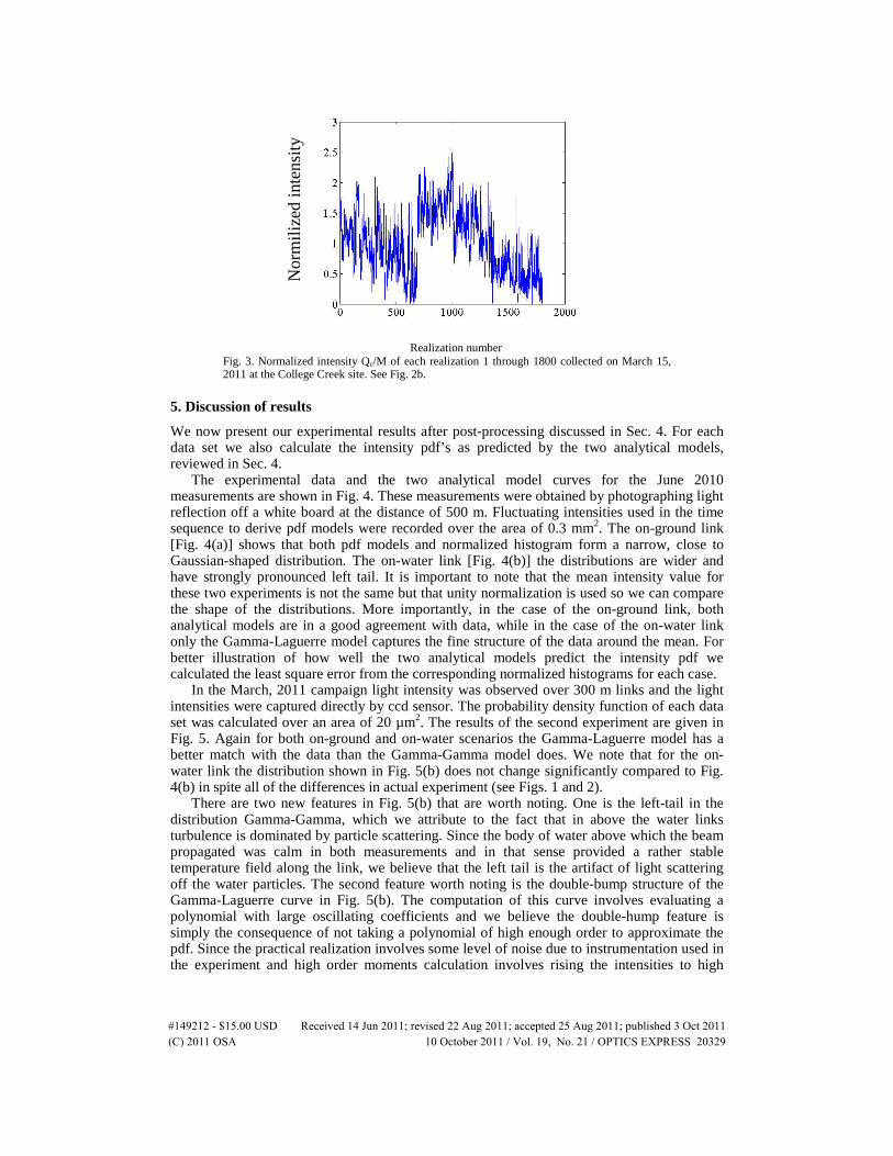
Fig. 3. Normalized intensity Qc/M of each realization 1 through 1800 collected on March 15, 2011 at the College Creek site. See Fig. 2b.

5. Discussion of results

We now present our experimental results after post-processing discussed in Sec. 4. For each data set we also calculate the intensity pdf’s as predicted by the two analytical models, reviewed in Sec. 4.

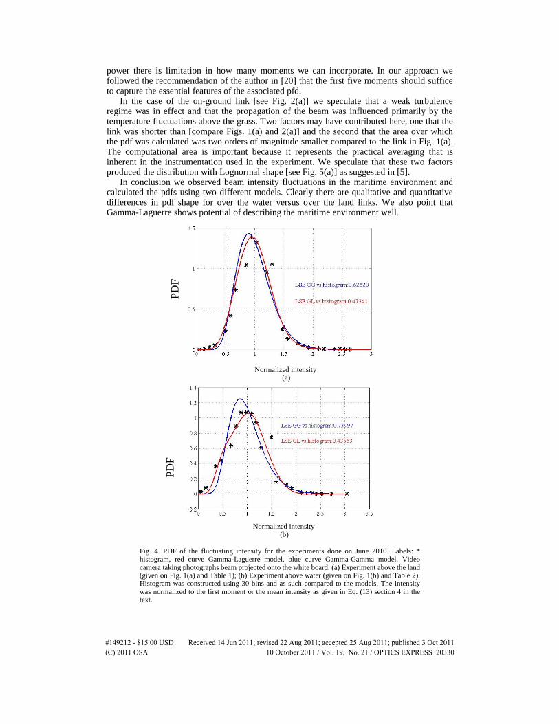
The experimental data and the two analytical model curves for the June 2010 measurements are shown in Fig. 4. These measurements were obtained by photographing light reflection off a white board at the distance of 500 m. Fluctuating intensities used in the time sequence to derive pdf models were recorded over the area of 0.3 mm2. The on-ground link [Fig. 4(a)] shows that both pdf models and normalized histogram form a narrow, close to Gaussian-shaped distribution. The on-water link [Fig. 4(b)] the distributions are wider and have strongly pronounced left tail. It is important to note that the mean intensity value for these two experiments is not the same but that unity normalization is used so we can compare the shape of the distributions. More importantly, in the case of the on-ground link, both analytical models are in a good agreement with data, while in the case of the on-water link only the Gamma-Laguerre model captures the fine structure of the data around the mean. For better illustration of how well the two analytical models predict the intensity pdf we calculated the least square error from the corresponding normalized histograms for each case.

In the March, 2011 campaign light intensity was observed over 300 m links and the light intensities were captured directly by ccd sensor. The probability density function of each data set was calculated over an area of 20 µm2. The results of the second experiment are given in Fig. 5. Again for both on-ground and on-water scenarios the Gamma-Laguerre model has a better match with the data than the Gamma-Gamma model does. We note that for the on-water link the distribution shown in Fig. 5(b) does not change significantly compared to Fig. 4(b) in spite all of the differences in actual experiment (see Figs. 1 and 2).

There are two new features in Fig. 5(b) that are worth noting. One is the left-tail in the distribution Gamma-Gamma, which we attribute to the fact that in above the water links turbulence is dominated by particle scattering. Since the body of water above which the beam propagated was calm in both measurements and in that sense provided a rather stable temperature field along the link, we believe that the left tail is the artifact of light scattering off the water particles. The second feature worth noting is the double-bump structure of the Gamma-Laguerre curve in Fig. 5(b). The computation of this curve involves evaluating a polynomial with large oscillating coefficients and we believe the double-hump feature is simply the consequence of not taking a polynomial of high enough order to approximate the pdf. Since the practical realization involves some level of noise due to instrumentation used in the experiment and high order moments calculation involves rising the intensities to high

Realization number

Nor

mili

zed

inte

nsity


power there is limitation in how many moments we can incorporate. In our approach we followed the recommendation of the author in [20] that the first five moments should suffice to capture the essential features of the associated pfd.

In the case of the on-ground link [see Fig. 2(a)] we speculate that a weak turbulence regime was in effect and that the propagation of the beam was influenced primarily by the temperature fluctuations above the grass. Two factors may have contributed here, one that the link was shorter than [compare Figs. 1(a) and 2(a)] and the second that the area over which the pdf was calculated was two orders of magnitude smaller compared to the link in Fig. 1(a). The computational area is important because it represents the practical averaging that is inherent in the instrumentation used in the experiment. We speculate that these two factors produced the distribution with Lognormal shape [see Fig. 5(a)] as suggested in [5].

In conclusion we observed beam intensity fluctuations in the maritime environment and calculated the pdfs using two different models. Clearly there are qualitative and quantitative differences in pdf shape for over the water versus over the land links. We also point that Gamma-Laguerre shows potential of describing the maritime environment well.

Fig. 4. PDF of the fluctuating intensity for the experiments done on June 2010. Labels: * histogram, red curve Gamma-Laguerre model, blue curve Gamma-Gamma model. Video camera taking photographs beam projected onto the white board. (a) Experiment above the land (given on Fig. 1(a) and Table 1); (b) Experiment above water (given on Fig. 1(b) and Table 2). Histogram was constructed using 30 bins and as such compared to the models. The intensity was normalized to the first moment or the mean intensity as given in Eq. (13) section 4 in the text.

PDF

PDF

Normalized intensity (a)

Normalized intensity (b)


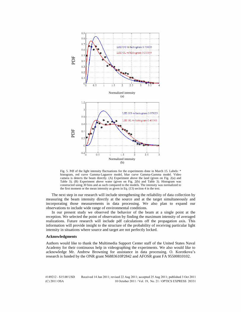
Fig. 5. Pdf of the light intensity fluctuations for the experiments done in March 15. Labels: * histogram, red curve Gamma-Laguerre model, blue curve Gamma-Gamma model. Video camera is detects the beam directly. (A) Experiment above the land (given on Fig. 2(a) and Table 3); (B) Experiment above water (given on Fig. 2(b) and Table 3). Histogram was constructed using 30 bins and as such compared to the models. The intensity was normalized to the first moment or the mean intensity as given in Eq. (13) section 4 in the text.

The next step in our research will include strengthening the reliability of data collection by measuring the beam intensity directly at the source and at the target simultaneously and incorporating those measurements in data processing. We also plan to expand our observations to include wide range of environmental conditions.

In our present study we observed the behavior of the beam at a single point at the reception. We selected the point of observation by finding the maximum intensity of averaged realizations. Future research will include pdf calculations off the propagation axis. This information will provide insight to the structure of the probability of receiving particular light intensity in situations where source and target are not perfectly locked.

Acknowledgments

Authors would like to thank the Multimedia Support Center staff of the United States Naval Academy for their continuous help in videographing the experiments. We also would like to acknowledge Mr. Andrew Browning for assistance in data processing. O. Korotkova’s research is funded by the ONR grant N6883610P2842 and AFOSR grant FA 95500810102.

PDF

Normalized intensity (a)

Normalized intensity (b)

PDF


Documents

Probability density function of the intensity of a laser ...Probability density function of the intensity of a laser beam propagating ... Vol. 2 of Methods of Modern Mathematical Physics