Probability distribution of orbital crossing times in a protoplanetary system

Earth Planets Space, 60, 681–691, 2008

Probability distribution of orbital crossing times in a protoplanetary system

Hiroyuki Emori1, Kiyoshi Nakazawa2, and Kazunori Iwasaki3

1Shumei University, Daigaku-Cho, Yachiyo-city, Chiba Prefecture, Japan2Tokyo Institute of Technology, 1-12-1 Oookayama, Meguro-ku, Tokyo, Japan

3Laboratory for Atomospheric and Space Physics, Univ. Colorado, 392, UCB Boulder, CO 80309-0392, USA

(Received June 4, 2007; Revised November 8, 2007; Accepted January 10, 2008; Online published July 4, 2008)

Long term behavior of five protoplanets was studied under the same conditions as those used in Chamberset al. (1996). One major difference was the number of calculations carried out for one parameter set of initialorbital distance. We reconfirmed their result for the orbital crossing times among five protoplanets starting fromcircular and co-planar orbits with an equal distance of their semi major axes. For each distance, the distributionof orbital crossing times was calculated from 500 sets of azimuthal positions of protoplanets randomly chosen.The distribution of the times around the average value resembles each other for almost all orbital distance cases.Based on a statistical certification we conclude that the fluctuations in orbital crossing times take “the log normalfunction”. The dispersion of the log normal distribution function is equal to 0.2. This means that 70% of theevents of orbital crossing occurs in the range between 10−0.2 times earlier and 100.2 times later than the averageorbital crossing time.Key words: Protoplanet, orbital crossing, planetary formation.

1. IntroductionIn the last decade we have made major advances in stud-

ies of planetary formation processes. This is especially truein terms of the accumulation of small planetesimals; wenow have the key to shorten time to build a protoplanet.This is “Run away growth” originally proposed by Wetherilland Stewart (1989). In the swarm of planetesimals, energyequipartition between bodies are established. This statis-tical mechanism determines the average random velocitiesas a decreasing function of mass of planetesimals. This iswell known as “dynamical friction” in the swarm (Stewartand Wetherill, 1988). Under the effect of the dynamicalfriction, the random velocity of protoplanets is suppressedto be much smaller than that of field planetesimals (Stew-art and Wetherill, 1988). In contrast, the random velocityof planetesimal is almost equal to the escape velocity fromone planetesimal. As a result, the relative velocity betweena large protoplanet and a small-field planetesimal is muchsmaller than the escape velocity from the protoplanet andthe ratio between these two velocities, which is called the“Safronov parameter” (Safronov, 1969), becomes larger asthe protoplanet grows. This increase in Savronov parame-ter enhances the collisional cross section of protoplanets toplanetesimals greatly, which is the run-away growth stage(Wetherill and Stewart, 1989).

Wetherill and Stewart (1989) were the first to propose therunaway growth, though they treated the swarm of planetes-imal as “particles in a box”, neglecting the effect of strongexternal solar gravity. Ida (1990) employed a sophisticated

Copyright c© The Society of Geomagnetism and Earth, Planetary and Space Sci-ences (SGEPSS); The Seismological Society of Japan; The Volcanological Societyof Japan; The Geodetic Society of Japan; The Japanese Society for Planetary Sci-ences; TERRAPUB.

theoretical formulation to treat gravitational scattering inthe solar gravitational field which he called “Hill approxi-mation” (Petit and Henon, 1987; Nakazawa and Ida, 1988),and confirmed that dynamical friction actually works, andthe runaway growth as well, in a swarm of planetesimalrevolving around the Sun. Ida estimates the accumulationtime of moon sized protoplanets in the earth region at lessthan one million years, though some questions remain, suchas “When does the runaway growth finish?”, “How are theprotoplanets distributed around the Sun after the processceased?”.

Kokubo and Ida (1998) were the first to study on thespacial distribution among planetesimal and protoplanetsduring the accumulation process. They carried out directorbital calculations, which is called “N-body simulations”,on the swarm of planetesimals. From their results, aboutten protoplanets with about Martian mass were produced inthe region of present-day Venus, Earth, and Mars orbits. Inaddition, the orbital distance between each protoplanet isalmost equal. This distance is about 10 mutual hill radius.Protoplanets are arranged to revolve in circular orbits at anequal distance in semi major axes. This is a condition ofprotoplanets just after the runaway growth stage.

Chambers et al. (1996) studied the behavior of protoplan-ets starting from the initial condition of protoplanets. Theyput five or more Martian-sized protoplanets in the present-day Venus, Earth, and Mars region. Initially the radial dis-tance between each orbit was set to be equal. The dis-tance was an important parameter in their study, as it isin our study. They then started orbital calculations. Dur-ing many orbital revolutions, protoplanets interact gravita-tionally with each other and increase their eccentricities.When a protoplanet reches an orbital eccentricity that islarge enough to approach an adjoining protoplanet, the pair

681

682 H. EMORI et al.: DISTRIBUTION OF ORBITAL CROSSING TIMES

of protoplanets can encounter each other in their mutual Hillsphere (Petit and Henon, 1987; Nakazawa and Ida, 1988).Chambers et al. called this event “orbital crossing”. Theiraim was to determine time needed for this orbital crossingevent as a function of orbital distance.

They put a parameter � to represent the initial orbitaldistance between each planet. They put five planets in fivecircular orbits around the sun. The difference in the semi-major axis between adjoining orbits was set to � times Hillradius, which is the radius of the mutual Hill sphere.

They pursued numerically the orbital evolution of plan-ets with changing � from 3.6 to 8.0, for every 0.2. For eachvalue of �, five cases of initial azimuthal conditions amongfive planets were examined. The most important results ofthe Chambers et al. (1996) study are that the orbital crossingtime depends on the orbital distance � exponentially. Ac-tually, from figure 1 in their work or Fig. 2(c) in this paper,though a fitting line show some considerable discrepanciesfrom data points, we can recognize that the orbital crossingtimes plotted logarithmically shows good linear correlationwith �.

Even if the initial orbital distance � is equal, the orbitalcrossing time becomes different owing to the difference inthe initial azimuthal positions. Chambers et al. (1996) re-ported that we have about one order of magnitude differencebetween maximum and minimum orbital crossing time foridentical values of �, in some cases.

The orbital crossing time depends strongly on the ini-tial orbital distance. Namely, unity increment in � resultsin about one order of magnitude elongation of the orbitalcrossing time. This result has a great importance on theplanetary formation process. Because protoplanets wereformed with distances about 10 Hill radius (Kokubo andIda, 1998), adopting their results to this case, the orbitalcrossing time was determined to be over one billion years.This long interval necessary for orbital crossing amongprotoplanets could make the time for planetary formationlonger than the life time of protoplanetary nebula gas whichis about several million years (Strom et al., 1993; Strom,1995). This raises some serious difficulties with the the-ory of Jovian planets formation (e.g. Mizuno et al., 1978;Ikoma et al., 2000). Owing to its importance to the studyof planetary formation theories, the relation of Chambers etal. has been studied by many authors after it was proposed.

One extension of Chambers law with breaking the initialcondition that all protoplanets have zero eccentricity was at-tempted by Yoshinaga et al. (1999). They initially pursuedorbital evolution of protoplanets which revolve around thesun along eccentric orbits and suggested that initial eccen-tricities make the orbital crossing time shorter than thosegiven by the Chambers law.

A strong perturbing source, namely Jupiter could havea large effect on the evolution of protoplanets around thepresent orbit of the Earth. Therefore if the Jovian planet isaccumulated earlier than terrestrial planets, we have to de-velop some new expressions on orbital crossing times. Be-cause Chambers et al. did not take Jupiter into account, Itoand Tanikawa (1999) considered a new relation between ini-tial orbital distance and orbital crossing time under the con-dition that there are already giant planets, namely Jupiter

and Saturn. They presented two important results: one isthat strong gravitational perturbation from the giant plan-ets effected a secular evolution on the eccentricities of pro-toplanets and made the orbital crossing time shorter thanthose in the case of no giant planets, the second is that a pro-toplanet, especially the protoplanet revolving on the mostouter orbit, could make an orbital crossing not only withother protoplanets but also with Jupiter. So the relation be-tween orbital distance and the orbital crossing time shouldbe changed in the specific case that the orbital distance islarge enough to make the most outer protoplanet approachthe giant planet easily.

As mentioned before planetary accretion processes havea strong relation to the random velocity of protoplanets andplanetesimals. The random velocity of planetesimals andprotoplanets are determined by the gravitational scatteringbetween them and some kinds of dissipative forces. Thegas drag force from protoplanetary nebula is the first candi-date for the dissipative force on protoplanets (Adachi et al.,1978). Although Chambers et al. supposed the protoplane-tary system in vacuum, it is a straightforward extension ofChambers et al. to consider the protoplanetary system in thegas nebula.

Iwasaki et al. (2001) studied the orbital crossing timefor the protoplanetary systems using the same approach asChambers et al. except that the former consider protoplan-ets revolving around the sun under the gas drag effects fromprotoplanetary nebula (e.g. Adachi et al., 1976). They stud-ied the behavior of protoplanets under a type of gas dragforce that is proportional to square of the random velocity,namely the Stokes-type gas drag. Gas drag force suppressesthe eccentricities of protoplanets, as such, protoplanets canhardly approach another one revolving on the adjoining or-bit. Iwasaki et al. (2001) presented a critical orbital dis-tance �c as a function of nebular gas densities that deter-mine the strength of the gas drag force. In the case that theorbital distance � is smaller than this critical value �c, theprotoplanet system has the orbital crossing event during alength of time which is almost equal to the orbital crossingtime given in Chambers et al. (1996). On the other hand,if the orbital distance exceeds the critical distance, the pro-toplanet system does not have any orbital crossing event,at least during a period which is one hundred times longerthan the orbital crossing time for the gas-free case.

In the same way, Iwasaki et al. (2002) studied the evolu-tion of protoplanets under the effect of another type of gasdrag force that is expressed to be proportional linearly tothe random velocity. They also presented the critical orbitaldistance �c in this case. For both cases of gas drag force thecritical orbital distance �c is determined from three piecesof information: the first is the intensity of the drag force, thesecond is orbital crossing time in the gas-free case, the thirdis stirring rate of random velocity given from three bodiesusing the distant encounter formulation by Hasegawa andNakazawa (1990), which is also formulated for the gas-freecase. This formula is very useful to study the orbital insta-bilities among protoplanets in nebula gas.

These studies focused on modifying of the Chambers etal. (1996) relation taking into account some additional fac-tors which should be considered in actual planetary for-

H. EMORI et al.: DISTRIBUTION OF ORBITAL CROSSING TIMES 683

mation processes. However, the most important question,‘Why does the Chambers relation exist?’ has never beenanswered. The relation is a purely empirical law obtainedfrom numerical experiments under some restricted initialconditions, namely zero eccentricities and equal orbital dis-tance. So, every time we want to break the restriction onthe initial conditions we have to again perform numerousorbital calculations on the protoplanetary system, as didChambers et al.

In other words, we need a theoretical model on the or-bital crossing time which can readily explain the Cham-bers relation under the condition that Chambers put in theirwork. This model would also allow us to estimate the or-bital crossing time in other cases than that of Chambers etal. (1996). We have already started a systematic study onthe evolution of protoplanets. The study starts with a recon-firmation of Chambers relation. The final goal is to obtaina theoretical model, as mentioned above. This paper is thefirst report based on this study.

The aim of this paper is twofold: (1) reconfirmationof the Chambers relation, (2) determination of distributionfunction of orbital crossing times, not only the average,which is our main purpose. Figure 1 in Chambers et al.(1996) suggests that orbital crossing times for identical ini-tial orbital distance possibly scatter in one order of mag-nitude range owing to the different initial azimuthal posi-tions of protoplanets. If so, it is very important to con-firm the distribution of orbital crossing times in one ensem-ble for which an initial orbital distance is assigned in orderto carry out discussions on the possible accumulation timeamong protoplanets. In addition, our study on the distri-bution may provide information on the elemental processesto produce the interesting Chambers relation on the averagevalue among the ensembles with different orbital distance�.

We therefore start with a reconfirmation of Chamberslaw. We explain our numerical simulation in brief in Sec-tion 2. This is almost same as that in Chambers et al. (1996).One different point is the number of trial runs executed forone parameter �. We carried out 500 runs for each param-eter �. The reason why we choose this number of sam-ples for one ensemble is explained in Appendix with a shortexplanation of a method in statistics called “KolmogorovSmilnov test”. In Section 3 we present our numerical re-sults. A comparison between our results and those in Cham-bers et al. are presented in detail. We can see that both setsof results fit well to each other. Our main result is that thedistribution of orbital crossing time is deduced from a num-ber of numerical results. In Section 4 we summarize ourresults and give the conclusions. Discussions are presentedin Section 5.

2. Basic Equations and Initial ConditionsThe basic equations in this study are the same to those

in Chambers et al. (1996). We consider five protoplanetsrevolving around the Sun. We will put them in sequentialnumber, beginning with the one nearest to the Sun.

Let us suppose the first planet, namely the planet with itsorbit nearest to the Sun, has a semi-major axis a0, initially.Hereafter we choose a0 as a unit of length. For other units,

we choose mass of the Sun, M�, as the unit of mass, and weset the unit of time to make Kepler frequency �0 defined as

�0 =√

GM�a3

0

(1)

to be equal to unity.Using the units mentioned above, the basic equations for

the five planets are written as

d2ri

dt2= − ri

r3i

+5∑

j�=i

mrj − ri∣∣rj − ri

∣∣3(2)

where ri is a vector from the center of the Sun to the positionof the i-th planet and m is mass of one planet. In thisequation we neglect the recoil term to the Sun from fiveplanets because their mass is much smaller than unity. Inthis study the mass of each planet is equal to each otherand we choose them to be equal to that in Chambers etal. (1996), which is about equal to the mass of Mercury.Because we choose the mass of the Sun as the unit of mass,we set m = 1 × 10−7.

As same as the mass of protoplanets, we choose the ini-tial conditions among them to be the same manner as inChambers et al. (1996). The semi-major axis of each planetis initially given in the following manner:

ai+1 = ai + �

(2m

3

)1/3 ai+1 + ai

2(3)

In this equation ai represents the semi-major axis of thei-th planet. As already mentioned, the first planet is theinnermost one, and its semi-major axis is chosen as a unitin this study. So, a1 = 1. From this condition and Eq. (3)we can obtain the semi-major axis from second to fifthplanets. In Eq. (3), � is an important parameter in thisstudy. We will examine the behavior of planets, placingdifferent initial conditions on �. We set it in the range from4.0 to 8.0.

All planets initially placed in a co-planer and circularKepler orbit. So, the initial eccentricities and inclinationsare given as

ei = ii = 0. (4)

Because all planets are in co-planer orbits, the inclinationsof planets are always equal to zero in this work. We there-fore consider 2-D problem only.

As we consider the 2-D problem, we need to specifyfour orbital elements to determine the initial conditions oneach planet. Semi-major axis and eccentricity are given inEqs. (3) and (4). The argument of perihelion and time ofperihelion passage is well known from other orbital ele-ments, though initial argument of perihelion can be set atan arbitrary value, because all planets are in circular orbits.So we put them as

�i = 0. (5)

It is more convenient to give the last initial condition asthe true anomaly of each planet than as the time of peri-helion passage. Here we introduce cylindrical coordinatescentered at the position of the Sun, and we represent radial


and azimuthal components of the i-th planet as ri and θi,respectively. As already mentioned, all planets are in circu-lar orbits initially. Therefore, the radial coordinate of i-thplanet is equal to it’s semi-major axis. The azimuthal com-ponent of the i-th planet is chosen randomly between zeroand 2π .

The parameter � in Eq. (3) is important in this study. Wechange it from 4.0 to 8.0 at 0.2 intervals. For each case of� we calculate 500 trial runs of the orbital evolution of thefive planets and make one ensemble. In each run, differentsets of five random numbers are generated to assign theazimuthal components of five planets.

We are now ready for numerical integration. We use the8-th order Runge-Kutta method with an algorithm for inte-gration of particles’ motion in strong external Solar gravityfield (Emori et al., 1994).

We pursue the orbital motion of five planets until a pairamong them approaches each other. When the distancebetween two planets becomes shorter than the two body Hillradius, h, defined as

h =(

2m

3

)1/3

(6)

(Nakazawa and Ida, 1988), we stop the calculation andrecord the time as the crossing time with the value of theparameter �. For one trial run, one orbital crossing timeis recorded. Because we execute 500 trial runs for onevalue of �, 500 crossing times is obtained for one caseof �. Using these 500 data points, the average crossingtime for � will be presented as in Chambers et al. (1996).In addition, we evaluate the distribution of crossing timearound the average value.

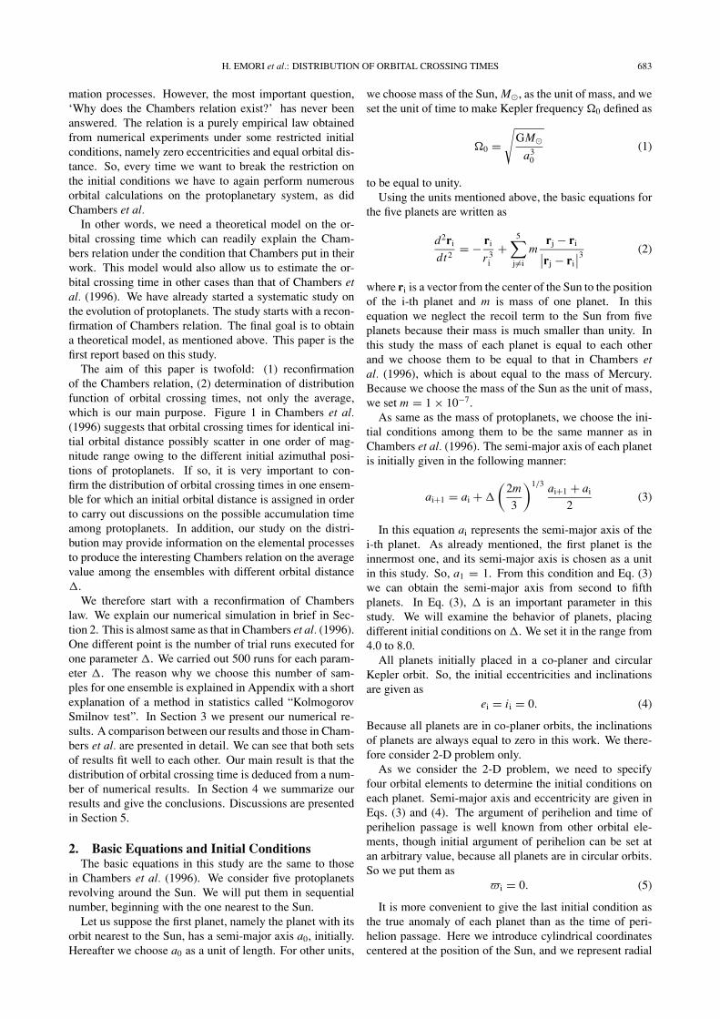
3. Numerical ResultsWe first present the time evolution of the orbits for five

protoplanets in a case of � equal to 6.0. In Fig. 1 wepresent the semi-major axis ai and eccentricity ei for eachplanet. Semi-major axes are expressed in Fig. 1(a), theeccentricities are expressed as the distance of the perihelionand aphelion in Fig. 1(b).

We plot (ai − 1)/h in Fig. 1(a) for five planets giventheir initial semi-major axis separated every �(= 6.0) asfunctions of time. They revolved around the Sun for about130,000 times. It takes 2π to revolve around the Sun atposition of r = 1 in our units of time and length. After sucha long period, a pair of planets, actually the second and thirdplanet in this case, approached each other and the distancebetween them became shorter than their mutual hill radiusdefined in Eq. (6). We then recorded the orbital crossingtime equal to 1.276 × 106.

Figure 1(a) reveals that the semi major axis of each planetkeeps its initial value just before the crossing time. Al-though semi-major axes of all planets show fluctuations inthe last 5% of total crossing time, the deviations are smallerthan the initial orbital separation �, which is equal to 6in the present case. Therefore, we conclude that the or-bital crossing between the second and third planets was notbrought about by fluctuations in their semi-major axes.

The reason of orbital crossing is well represented inFig. 1(b). In this figure we plot two values namely (ai(1 +

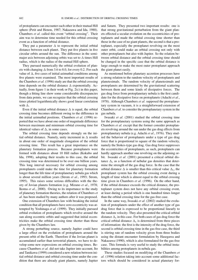
Fig. 1. Orbital evolution of five protoplanets. Mass of a planet and initialdistance of semi-major axis between each planet are 1.0e−7 and 6.0,respectively. In panel (a) semi-major axis of each planet is drawn. Inpanel (b) radial distance of the perihelion and the aphelion of each planetare presented. Horizontal axis is time in both panels. In horizontalaxis time is presented in the unit of 2π , which is equal to 1 year if thereference orbit is chosen as a0 = 1 [AU].

ei) − 1)/h and (ai(1 − ei) − 1)/h), where h is the mutualHill radius defined in Eq. (6), for each planet as functionsof time. The former is the radial distance between the ori-gin of coordinates and the perihelion of i-th planet, and thelatter is that of aphelion. So the half of the width betweentwo lines is equal to the eccentricity of each planet. Con-trary to the evolution of semi-major axes, the eccentricitiesof planets increased from an initial value zero continuouslywith time, though the rates of increase enlarge abruptly at95% of the total crossing time. In the last 5% of crossingtime, the eccentricities of planets grow steeply. As a result,a perihelion of a planet moves inward and steps over theaphelion of its inner neighboring planet. In the case of thisfigure, the two orbits of the second and third planet crosseseach other owing to the fact that their eccentricities growlarge enough to compensate their initial radial distance �.

Iwasaki et al. (2001) have already reported a gradual in-crease in eccentricities and a sudden jump in a short period


2

4

6

8

log

t c

3 4 5 6 7 8

(a)

2

4

6

8

3 4 5 6 7 8

(c)

0.0

0.2

0.4

3 4 5 6 7 8

(b)

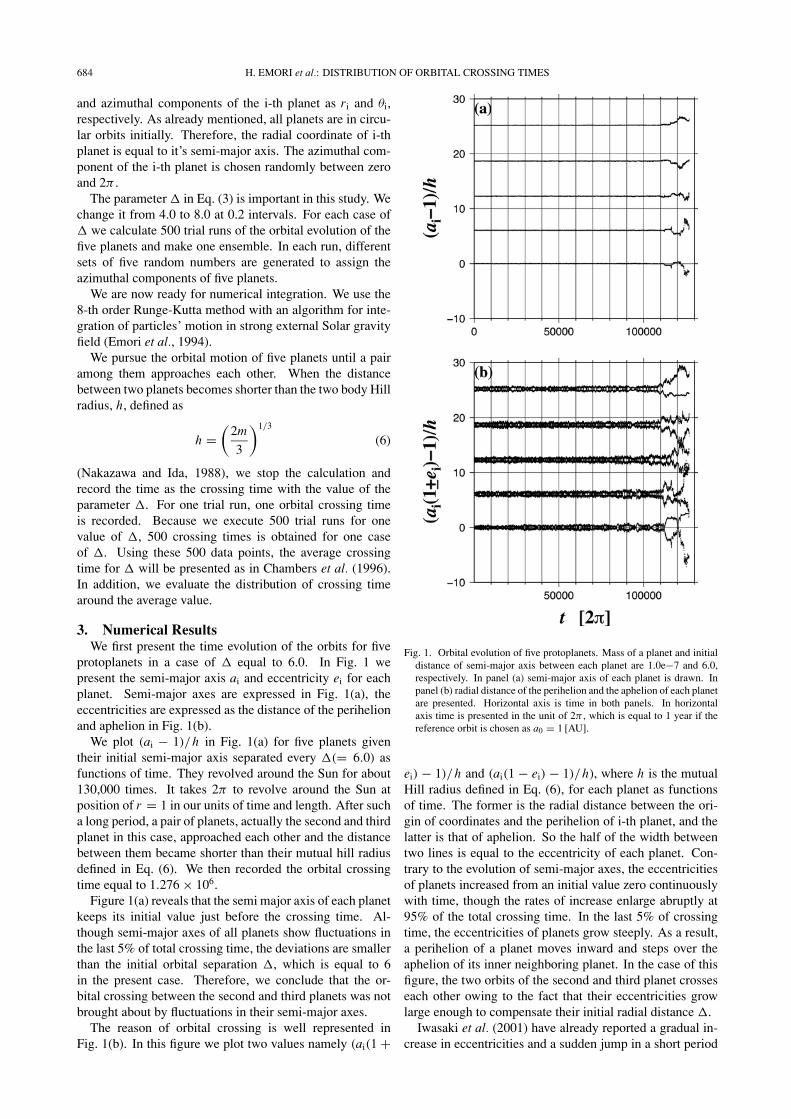
Fig. 2. In panel (a), averaged orbital crossing time obtained from 500 ensembles for each � is presented with dispersion. Average value and dispersionare defined in Eqs. (7) and (8), respectively. Average value is presented with a circle, and dispersion corresponds to half the length of the vertical bardrawn on the circle. In panel (b), the dispersion is presented as a function of �. For comparison, in panel (c) we redraw results presented in Chamberset al. (1996) for the case that five protoplanets each of them has 1 × 10−7 M� as same as this work.

just before the orbital crossing time. Our results are on com-mon ground about this point.

For one parameter � we carried out 500 trial runs withchanging initial azimuthal angle for each planet. In eachrun we obtain the orbital crossing time in a same mannerexplained for Fig. 1. Therefore, we obtain 500 differentorbital crossing times for one parameter �.

In Fig. 2(a) we represent average and dispersion calcu-lated from 500 orbital crossing times for each value of �

from 4.0 to 8.0 every 0.2 interval. An average of orbitalcrossing time is defined as

〈log(tc)〉� = 1

500

500∑

k=1

log(tc(�; k)) (7)

where tc(�; k) is an orbital crossing time obtained in thek-th trial run in the ensemble for the case of orbital distanceparameter �. After the average was obtained, we obtain thedispersion for the case of � as

σ(�) =√√√√ 1

500

500∑

k=1

(log(tc(�; k)) − 〈log(tc)〉�)2. (8)

In Fig. 2, mean values of orbital crossing time 〈log(tc)〉�is plotted (open circles) and σ(�) are represented by halflength of each short line stretching upward and downwardfrom each average value point.

We re-confirm the results shown in figure 2 of Chamberset al. (1997) from our Fig. 2(a) and (c). As they pointed out,the average values are well approximated by a linear line onthis plane. Therefore, the average of orbital crossing time

depends roughly on the parameter � exponentially. Notonly this characteristic feature of average orbital crossingtime, but also other details shown on the figure, for examplepositions and magnitudes of many bumps show good agree-ment to the result in Chambers et al. Iwasaki et al. (2001)studied the orbital crossing time in the case that protoplan-ets revolve in the gaseous nebula, however, they presentthe orbital crossing time in the gas-free case for discussion.Comparing their figure (figure 2 in Iwasaki et al. (2001))provides re-confirmation of the results in Chambers et al.

The number of the trial runs for the initial azimuthalpositions of five protoplanets in both Chambers et al. andIwasaki et al. is equal to five. So, we found that five runsfor each case of � is enough to obtain the average value oforbital crossing time. This fact suggests that the distributionfunctions of orbital crossing time in every case of parameter� may have one sharp peak around each average.

As seen in Fig. 2(a), σ(�) are almost equal to each other.We draw σ(�) as a function of � in Fig. 2(b). Dispersionsof orbital crossing times are equal to 0.2 as long as � is inthe range of 4.0 to 5.0. It begins fluctuating as � becomeslower than 5.0. At last σ(�) distributes between 0.15 and0.25 in the range of � between 6.0 and 8.0. Looking atthe average orbital crossing times in Fig. 2(a), we recog-nize that 〈log(tc)〉� can be approximated very well by a linein the range of � smaller than 5.0. Though, as with thefluctuation in the case of σ(�), in the range of � greaterthan 5.0, 〈log(tc)〉� begins to deviate from the fitting line.Furthermore, it becomes difficult to approximate the aver-ages of orbital crossing time by one line in the range of �

larger than 6.0. To elusidate these behaviors of 〈log(tc)〉�


0.0

0.2

0.4

0.6

0.8

1.0

2 3 4 5 6

log tc

=4 =5 =6

(a)

0.0

0.2

0.4

0.6

0.8

1.0

-2 -1 0 1 2

log tc-<log tc>

(b)

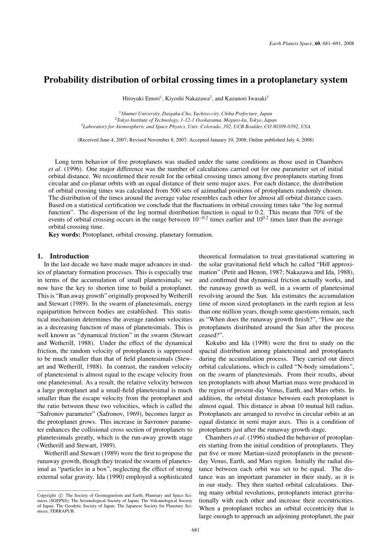
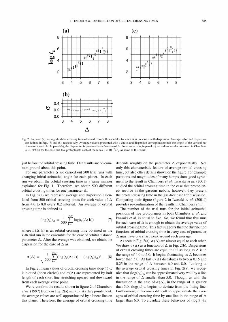
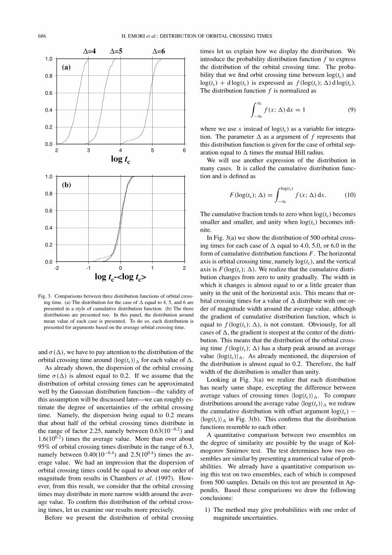
Fig. 3. Comparisons between three distribution functions of orbital cross-ing time. (a) The distribution for the case of � equal to 4, 5, and 6 arepresented in a style of cumulative distribution function. (b) The threedistributions are presented too. In this panel, the distribution aroundmean value of each case is presented. To do so, each distribution ispresented for arguments based on the average orbital crossing time.

and σ(�), we have to pay attention to the distribution of theorbital crossing time around 〈log(tc)〉� for each value of �.

As already shown, the dispersion of the orbital crossingtime σ(�) is almost equal to 0.2. If we assume that thedistribution of orbital crossing times can be approximatedwell by the Gaussian distribution function—the validity ofthis assumption will be discussed later—we can roughly es-timate the degree of uncertainties of the orbital crossingtime. Namely, the dispersion being equal to 0.2 meansthat about half of the orbital crossing times distribute inthe range of factor 2.25, namely between 0.63(10−0.2) and1.6(100.2) times the average value. More than over about95% of orbital crossing times distribute in the range of 6.3,namely between 0.40(10−0.4) and 2.5(100.4) times the av-erage value. We had an impression that the dispersion oforbital crossing times could be equal to about one order ofmagnitude from results in Chambers et al. (1997). How-ever, from this result, we consider that the orbital crossingtimes may distribute in more narrow width around the aver-age value. To confirm this distribution of the orbital cross-ing times, let us examine our results more precisely.

Before we present the distribution of orbital crossing

times let us explain how we display the distribution. Weintroduce the probability distribution function f to expressthe distribution of the orbital crossing time. The proba-bility that we find orbit crossing time between log(tc) andlog(tc) + d log(tc) is expressed as f (log(tc); �) d log(tc).The distribution function f is normalized as

∫ ∞

−∞f (x; �) dx = 1 (9)

where we use x instead of log(tc) as a variable for integra-tion. The parameter � as a argument of f represents thatthis distribution function is given for the case of orbital sep-aration equal to � times the mutual Hill radius.

We will use another expression of the distribution inmany cases. It is called the cumulative distribution func-tion and is defined as

F(log(tc); �) =∫ log(tc)

−∞f (x; �) dx . (10)

The cumulative fraction tends to zero when log(tc) becomessmaller and smaller, and unity when log(tc) becomes infi-nite.

In Fig. 3(a) we show the distribution of 500 orbital cross-ing times for each case of � equal to 4.0, 5.0, or 6.0 in theform of cumulative distribution functions F . The horizontalaxis is orbital crossing time, namely log(tc), and the verticalaxis is F(log(tc); �). We realize that the cumulative distri-bution changes from zero to unity gradually. The width inwhich it changes is almost equal to or a little greater thanunity in the unit of the horizontal axis. This means that or-bital crossing times for a value of � distribute with one or-der of magnitude width around the average value, althoughthe gradient of cumulative distribution function, which isequal to f (log(tc); �), is not constant. Obviously, for allcases of �, the gradient is steepest at the center of the distri-bution. This means that the distribution of the orbital cross-ing time f (log(tc); �) has a sharp peak around an averagevalue 〈log(tc)〉�. As already mentioned, the dispersion ofthe distribution is almost equal to 0.2. Therefore, the halfwidth of the distribution is smaller than unity.

Looking at Fig. 3(a) we realize that each distributionhas nearly same shape, excepting the difference betweenaverage values of crossing times 〈log(tc)〉�. To comparedistributions around the average value 〈log(tc)〉� we redrawthe cumulative distribution with offset argument log(tc) −〈log(tc)〉� in Fig. 3(b). This confirms that the distributionfunctions resemble to each other.

A quantitative comparison between two ensembles onthe degree of similarity are possible by the usage of Kol-mogorov Smirnov test. The test determines how two en-sembles are similar by presenting a numerical value of prob-abilities. We already have a quantitative comparison us-ing this test on two ensembles, each of which is composedfrom 500 samples. Details on this test are presented in Ap-pendix. Based these comparisons we draw the followingconclusions:

1) The method may give probabilities with one order ofmagnitude uncertainties.


Table 1. Probabilities obtained by Kolmogorov Smirnov test comparingensembles for � = 4.0, 5.0, and 6.0.

� 5.0 6.04.0 4.60e−1 4.16e−25.0 — 4.76e−3

4

5

6

7

8

4 5 6 7 8

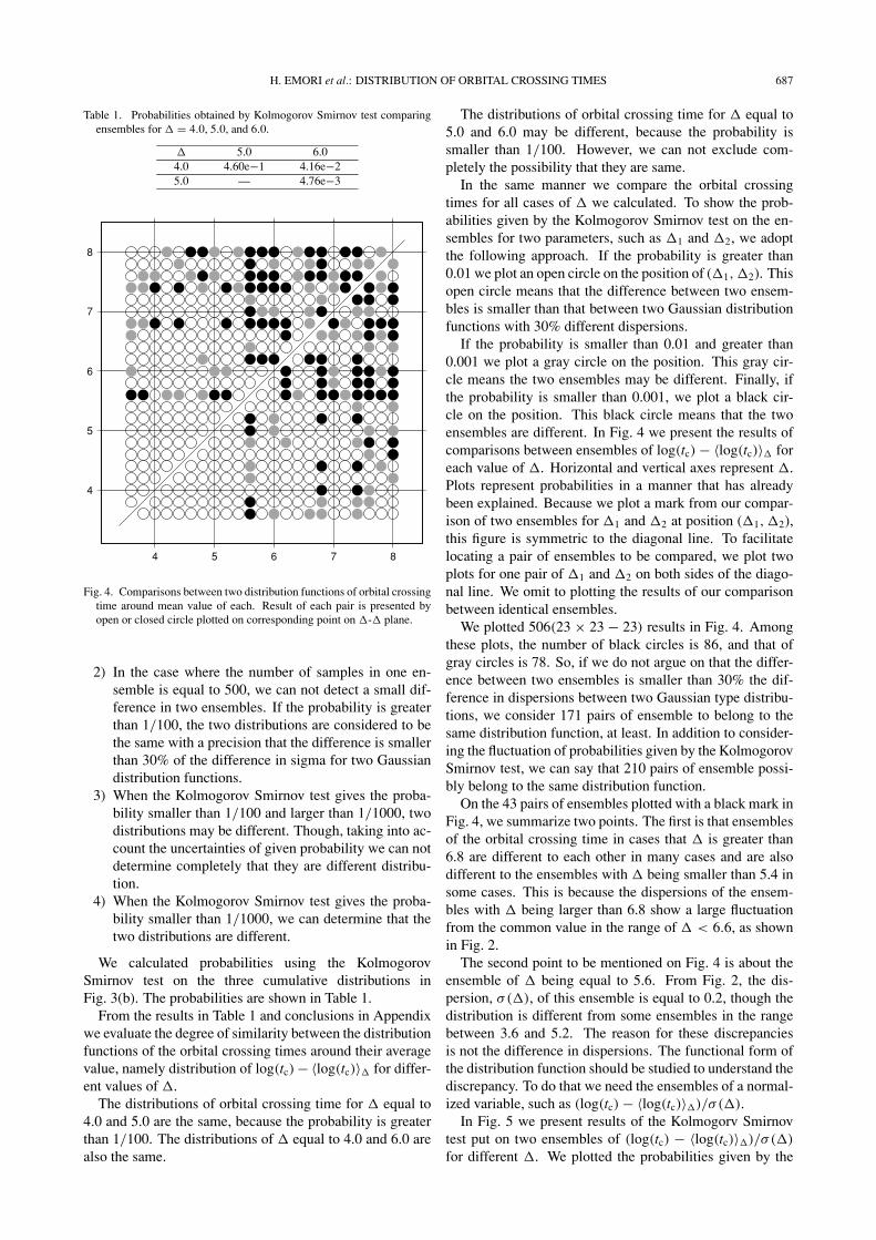
Fig. 4. Comparisons between two distribution functions of orbital crossingtime around mean value of each. Result of each pair is presented byopen or closed circle plotted on corresponding point on �-� plane.

2) In the case where the number of samples in one en-semble is equal to 500, we can not detect a small dif-ference in two ensembles. If the probability is greaterthan 1/100, the two distributions are considered to bethe same with a precision that the difference is smallerthan 30% of the difference in sigma for two Gaussiandistribution functions.

3) When the Kolmogorov Smirnov test gives the proba-bility smaller than 1/100 and larger than 1/1000, twodistributions may be different. Though, taking into ac-count the uncertainties of given probability we can notdetermine completely that they are different distribu-tion.

4) When the Kolmogorov Smirnov test gives the proba-bility smaller than 1/1000, we can determine that thetwo distributions are different.

We calculated probabilities using the KolmogorovSmirnov test on the three cumulative distributions inFig. 3(b). The probabilities are shown in Table 1.

From the results in Table 1 and conclusions in Appendixwe evaluate the degree of similarity between the distributionfunctions of the orbital crossing times around their averagevalue, namely distribution of log(tc) − 〈log(tc)〉� for differ-ent values of �.

The distributions of orbital crossing time for � equal to4.0 and 5.0 are the same, because the probability is greaterthan 1/100. The distributions of � equal to 4.0 and 6.0 arealso the same.

The distributions of orbital crossing time for � equal to5.0 and 6.0 may be different, because the probability issmaller than 1/100. However, we can not exclude com-pletely the possibility that they are same.

In the same manner we compare the orbital crossingtimes for all cases of � we calculated. To show the prob-abilities given by the Kolmogorov Smirnov test on the en-sembles for two parameters, such as �1 and �2, we adoptthe following approach. If the probability is greater than0.01 we plot an open circle on the position of (�1, �2). Thisopen circle means that the difference between two ensem-bles is smaller than that between two Gaussian distributionfunctions with 30% different dispersions.

If the probability is smaller than 0.01 and greater than0.001 we plot a gray circle on the position. This gray cir-cle means the two ensembles may be different. Finally, ifthe probability is smaller than 0.001, we plot a black cir-cle on the position. This black circle means that the twoensembles are different. In Fig. 4 we present the results ofcomparisons between ensembles of log(tc) − 〈log(tc)〉� foreach value of �. Horizontal and vertical axes represent �.Plots represent probabilities in a manner that has alreadybeen explained. Because we plot a mark from our compar-ison of two ensembles for �1 and �2 at position (�1, �2),this figure is symmetric to the diagonal line. To facilitatelocating a pair of ensembles to be compared, we plot twoplots for one pair of �1 and �2 on both sides of the diago-nal line. We omit to plotting the results of our comparisonbetween identical ensembles.

We plotted 506(23 × 23 − 23) results in Fig. 4. Amongthese plots, the number of black circles is 86, and that ofgray circles is 78. So, if we do not argue on that the differ-ence between two ensembles is smaller than 30% the dif-ference in dispersions between two Gaussian type distribu-tions, we consider 171 pairs of ensemble to belong to thesame distribution function, at least. In addition to consider-ing the fluctuation of probabilities given by the KolmogorovSmirnov test, we can say that 210 pairs of ensemble possi-bly belong to the same distribution function.

On the 43 pairs of ensembles plotted with a black mark inFig. 4, we summarize two points. The first is that ensemblesof the orbital crossing time in cases that � is greater than6.8 are different to each other in many cases and are alsodifferent to the ensembles with � being smaller than 5.4 insome cases. This is because the dispersions of the ensem-bles with � being larger than 6.8 show a large fluctuationfrom the common value in the range of � < 6.6, as shownin Fig. 2.

The second point to be mentioned on Fig. 4 is about theensemble of � being equal to 5.6. From Fig. 2, the dis-persion, σ(�), of this ensemble is equal to 0.2, though thedistribution is different from some ensembles in the rangebetween 3.6 and 5.2. The reason for these discrepanciesis not the difference in dispersions. The functional form ofthe distribution function should be studied to understand thediscrepancy. To do that we need the ensembles of a normal-ized variable, such as (log(tc) − 〈log(tc)〉�)/σ(�).

In Fig. 5 we present results of the Kolmogorv Smirnovtest put on two ensembles of (log(tc) − 〈log(tc)〉�)/σ(�)

for different �. We plotted the probabilities given by the


4

5

6

7

8

4 5 6 7 8

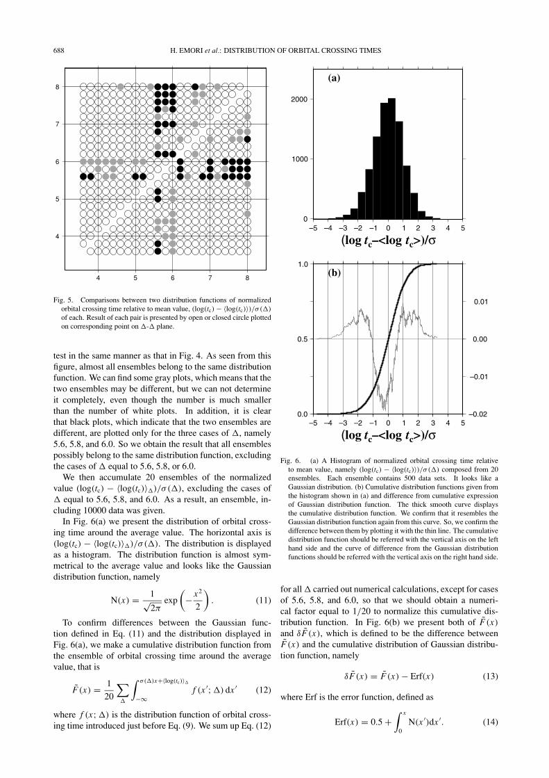
Fig. 5. Comparisons between two distribution functions of normalizedorbital crossing time relative to mean value, (log(tc) − 〈log(tc)〉)/σ (�)

of each. Result of each pair is presented by open or closed circle plottedon corresponding point on �-� plane.

test in the same manner as that in Fig. 4. As seen from thisfigure, almost all ensembles belong to the same distributionfunction. We can find some gray plots, which means that thetwo ensembles may be different, but we can not determineit completely, even though the number is much smallerthan the number of white plots. In addition, it is clearthat black plots, which indicate that the two ensembles aredifferent, are plotted only for the three cases of �, namely5.6, 5.8, and 6.0. So we obtain the result that all ensemblespossibly belong to the same distribution function, excludingthe cases of � equal to 5.6, 5.8, or 6.0.

We then accumulate 20 ensembles of the normalizedvalue (log(tc) − 〈log(tc)〉�)/σ(�), excluding the cases of� equal to 5.6, 5.8, and 6.0. As a result, an ensemble, in-cluding 10000 data was given.

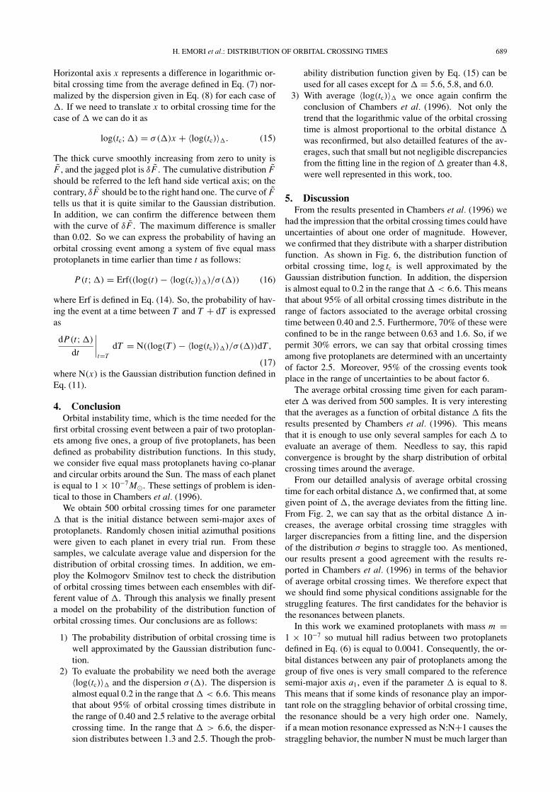
In Fig. 6(a) we present the distribution of orbital cross-ing time around the average value. The horizontal axis is(log(tc) − 〈log(tc)〉�)/σ(�). The distribution is displayedas a histogram. The distribution function is almost sym-metrical to the average value and looks like the Gaussiandistribution function, namely

N(x) = 1√2π

exp

(− x2

2

). (11)

To confirm differences between the Gaussian func-tion defined in Eq. (11) and the distribution displayed inFig. 6(a), we make a cumulative distribution function fromthe ensemble of orbital crossing time around the averagevalue, that is

F̃(x) = 1

20

∑

�

∫ σ(�)x+〈log(tc)〉�

−∞f (x ′; �) dx ′ (12)

where f (x; �) is the distribution function of orbital cross-ing time introduced just before Eq. (9). We sum up Eq. (12)

Fig. 6. (a) A Histogram of normalized orbital crossing time relativeto mean value, namely (log(tc) − 〈log(tc)〉)/σ (�) composed from 20ensembles. Each ensemble contains 500 data sets. It looks like aGaussian distribution. (b) Cumulative distribution functions given fromthe histogram shown in (a) and difference from cumulative expressionof Gaussian distribution function. The thick smooth curve displaysthe cumulative distribution function. We confirm that it resembles theGaussian distribution function again from this curve. So, we confirm thedifference between them by plotting it with the thin line. The cumulativedistribution function should be referred with the vertical axis on the lefthand side and the curve of difference from the Gaussian distributionfunctions should be referred with the vertical axis on the right hand side.

for all � carried out numerical calculations, except for casesof 5.6, 5.8, and 6.0, so that we should obtain a numeri-cal factor equal to 1/20 to normalize this cumulative dis-tribution function. In Fig. 6(b) we present both of F̃(x)

and δ F̃(x), which is defined to be the difference betweenF̃(x) and the cumulative distribution of Gaussian distribu-tion function, namely

δ F̃(x) = F̃(x) − Erf(x) (13)

where Erf is the error function, defined as

Erf(x) = 0.5 +∫ x

0N(x ′)dx ′. (14)


Horizontal axis x represents a difference in logarithmic or-bital crossing time from the average defined in Eq. (7) nor-malized by the dispersion given in Eq. (8) for each case of�. If we need to translate x to orbital crossing time for thecase of � we can do it as

log(tc; �) = σ(�)x + 〈log(tc)〉�. (15)

The thick curve smoothly increasing from zero to unity isF̃ , and the jagged plot is δ F̃ . The cumulative distribution F̃should be referred to the left hand side vertical axis; on thecontrary, δ F̃ should be to the right hand one. The curve of F̃tells us that it is quite similar to the Gaussian distribution.In addition, we can confirm the difference between themwith the curve of δ F̃ . The maximum difference is smallerthan 0.02. So we can express the probability of having anorbital crossing event among a system of five equal massprotoplanets in time earlier than time t as follows:

P(t; �) = Erf((log(t) − 〈log(tc)〉�)/σ(�)) (16)

where Erf is defined in Eq. (14). So, the probability of hav-ing the event at a time between T and T + dT is expressedas

dP(t; �)

dt

∣∣∣∣t=T

dT = N((log(T ) − 〈log(tc)〉�)/σ(�))dT,

(17)where N(x) is the Gaussian distribution function defined inEq. (11).

4. ConclusionOrbital instability time, which is the time needed for the

first orbital crossing event between a pair of two protoplan-ets among five ones, a group of five protoplanets, has beendefined as probability distribution functions. In this study,we consider five equal mass protoplanets having co-planarand circular orbits around the Sun. The mass of each planetis equal to 1 × 10−7 M�. These settings of problem is iden-tical to those in Chambers et al. (1996).

We obtain 500 orbital crossing times for one parameter� that is the initial distance between semi-major axes ofprotoplanets. Randomly chosen initial azimuthal positionswere given to each planet in every trial run. From thesesamples, we calculate average value and dispersion for thedistribution of orbital crossing times. In addition, we em-ploy the Kolmogorv Smilnov test to check the distributionof orbital crossing times between each ensembles with dif-ferent value of �. Through this analysis we finally presenta model on the probability of the distribution function oforbital crossing times. Our conclusions are as follows:

1) The probability distribution of orbital crossing time iswell approximated by the Gaussian distribution func-tion.

2) To evaluate the probability we need both the average〈log(tc)〉� and the dispersion σ(�). The dispersion isalmost equal 0.2 in the range that � < 6.6. This meansthat about 95% of orbital crossing times distribute inthe range of 0.40 and 2.5 relative to the average orbitalcrossing time. In the range that � > 6.6, the disper-sion distributes between 1.3 and 2.5. Though the prob-

ability distribution function given by Eq. (15) can beused for all cases except for � = 5.6, 5.8, and 6.0.

3) With average 〈log(tc)〉� we once again confirm theconclusion of Chambers et al. (1996). Not only thetrend that the logarithmic value of the orbital crossingtime is almost proportional to the orbital distance �

was reconfirmed, but also detailled features of the av-erages, such that small but not negligible discrepanciesfrom the fitting line in the region of � greater than 4.8,were well represented in this work, too.

5. DiscussionFrom the results presented in Chambers et al. (1996) we

had the impression that the orbital crossing times could haveuncertainties of about one order of magnitude. However,we confirmed that they distribute with a sharper distributionfunction. As shown in Fig. 6, the distribution function oforbital crossing time, log tc is well approximated by theGaussian distribution function. In addition, the dispersionis almost equal to 0.2 in the range that � < 6.6. This meansthat about 95% of all orbital crossing times distribute in therange of factors associated to the average orbital crossingtime between 0.40 and 2.5. Furthermore, 70% of these wereconfined to be in the range between 0.63 and 1.6. So, if wepermit 30% errors, we can say that orbital crossing timesamong five protoplanets are determined with an uncertaintyof factor 2.5. Moreover, 95% of the crossing events tookplace in the range of uncertainties to be about factor 6.

The average orbital crossing time given for each param-eter � was derived from 500 samples. It is very interestingthat the averages as a function of orbital distance � fits theresults presented by Chambers et al. (1996). This meansthat it is enough to use only several samples for each � toevaluate an average of them. Needless to say, this rapidconvergence is brought by the sharp distribution of orbitalcrossing times around the average.

From our detailled analysis of average orbital crossingtime for each orbital distance �, we confirmed that, at somegiven point of �, the average deviates from the fitting line.From Fig. 2, we can say that as the orbital distance � in-creases, the average orbital crossing time straggles withlarger discrepancies from a fitting line, and the dispersionof the distribution σ begins to straggle too. As mentioned,our results present a good agreement with the results re-ported in Chambers et al. (1996) in terms of the behaviorof average orbital crossing times. We therefore expect thatwe should find some physical conditions assignable for thestruggling features. The first candidates for the behavior isthe resonances between planets.

In this work we examined protoplanets with mass m =1 × 10−7 so mutual hill radius between two protoplanetsdefined in Eq. (6) is equal to 0.0041. Consequently, the or-bital distances between any pair of protoplanets among thegroup of five ones is very small compared to the referencesemi-major axis a1, even if the parameter � is equal to 8.This means that if some kinds of resonance play an impor-tant role on the straggling behavior of orbital crossing time,the resonance should be a very high order one. Namely,if a mean motion resonance expressed as N:N+1 causes thestraggling behavior, the number N must be much larger than


unity. It is not clear whether such higher order resonancescan contribute to the orbital behavior of protoplanets.

Although the distribution of orbital crossing times is pre-sented in this work, there are still some problems in the or-bital evolution of protoplanets. The straggling behavior isone of them. Therefore we need more studies on this theme.We have started our studies with one on the protoplanet sys-tem with wide range of protoplanet mass parameter. If weconsider two systems of protoplanets with three orders ofmagnitude difference in planets mass, the orbital distancebetween two protoplanets in each system is different withone order of magnitude, even if the parameter � is equalto each other. The contribution of some kinds of resonancewill be examined in this future study as wide mass parame-ter.

Another future problem is that some kinds of resonancebetween a protoplanet and other extra perturbing source,namely Jovian planets, are important. In the study of ter-restrial planet formation, this effect may be taken as an keyprocess. We have already had a report on the average or-bital crossing times that the time is shortened by the extraperturbation (Ito and Tanikawa, 1999). As yet, no studieshave been carried out on the distribution of the orbital cross-ing times under such conditions. It is very difficult to inferthe effect of extra perturbations on the distribution function,though we expect that we can do it if we have a theoreticalmodel of orbital evolution of protoplanets, which we willattempt to construct in future studies.

Acknowledgments. The authors have appreciated fruitful discus-sions with members of the Nakazawa Laboratory, Tokyo Instituteof Technology. A part of the numerical simulations carried outin this work were carried out in the GSIC in Tokyo Institute ofTechnology. This work is supported by a Grant-in-Aid for Scien-tific Research (C) No. 16540382 brought by Japan Society of thePromotion of Science.

Appendix A. Kolmogorov Smirnov TestIn this study we use the “Kolmogorov Smirnov test”

(Press et al., 1986) to confirm whether two ensembles oforbital crossing times belong to one distribution function ornot. Let us explain the procedure in this method briefly.Suppose that there are two distribution functions expressedin a style of the cumulative probability function, each ofwhich is composed from finite number samples. At first welook for the maximum difference between these two distri-bution functions. Let us express this with δ. Next by theusage of the equation defined as

P = 2∞∑

j=1

(−1)j exp

(−(

N1N2

N1 + N2

)δ2 j2

)(A.1)

where N1 and N2 is number of data in ensemble 1 and 2,respectively. From this equation we obtain probability P .

If P is equal to unity, the two distribution functions arecompletely same. On the other hand, in the case that P isequal to zero, the two distributions are completely different.

If we compare two ensembles with a finite number ofsamples, we may never find this Kolmogorov Smirnov testgiving the probability being equal to unity. This is becauseeven if two ensembles belong to same distribution function,a finite sample number should bring some differences intwo cumulative distribution functions. For example, let usgenerate two sets of ensembles which are composed fromsamples brought from a Gaussian distribution function andcompare them with the method. The Gaussian distributionfunction has dispersion σ equal to 1.0. The ensembles areas follows;

1) Generate 500 random numbers between 0 and 1. Letus denote them as xi.

2) For each random number we calculate vi which satis-fies the following condition:

xi = (1 + Erf(vi/2σ))/2

where Erf is the error function.

Through this procedure with 11 different sets of randomnumbers, we construct 11 ensembles for the same disper-sion σ = 1.0, then we compare the first and each of theother ten ensembles. In Table 2 we present ten probabilitiesobtained from these comparisons.

As seen from Table 2, the probabilities distribute between0.67 and 0.029. From this fact, we must notice that themethod gives probabilities with over one order of magni-tude uncertainties, even for comparisons between sampleswith one identical distribution function. So, in a case thatwe compare two unknown ensembles we can not easily de-cide the two ensembles belong to different distribution func-tions even if the probability is smaller than 1.0.

We therefore need some quantitative comparisons be-tween differences in two ensembles and the probabilitiesgiven by Kolmogorov Smirnov tests. Let us therefore com-pare two ensembles selected from two Gaussian distribu-tions with different dispersion σ . From these data, wepresent a relation between differences in dispersion and theprobability given by Kolmogorov Smirnov test.

Our first step is to construct one ensemble composedfrom 500 samples randomly selected from a Gaussian dis-tribution function with σ equal to 1.0. We call this ensembleour reference ensemble. Next we construct 20 ensembles,each of which is composed of 500 samples randomly se-lected from a Gaussian distribution function with same σ

equal to 1.0. We call these ensembles our test ensembles.We compare the reference ensemble and each of the test en-sembles, and obtain 20 probabilities. We then obtain theaverage of these. In the case of a comparison of two ensem-bles of which the components are sampled from a Gaussian

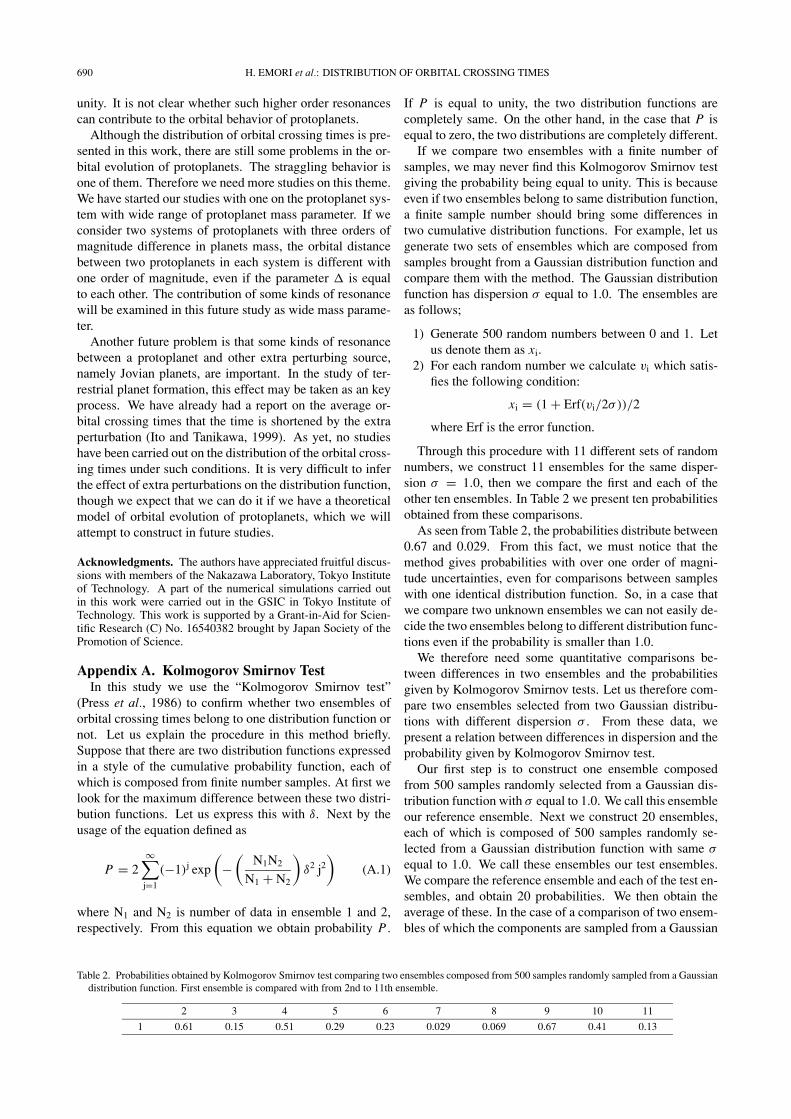
Table 2. Probabilities obtained by Kolmogorov Smirnov test comparing two ensembles composed from 500 samples randomly sampled from a Gaussiandistribution function. First ensemble is compared with from 2nd to 11th ensemble.

2 3 4 5 6 7 8 9 10 11

1 0.61 0.15 0.51 0.29 0.23 0.029 0.069 0.67 0.41 0.13


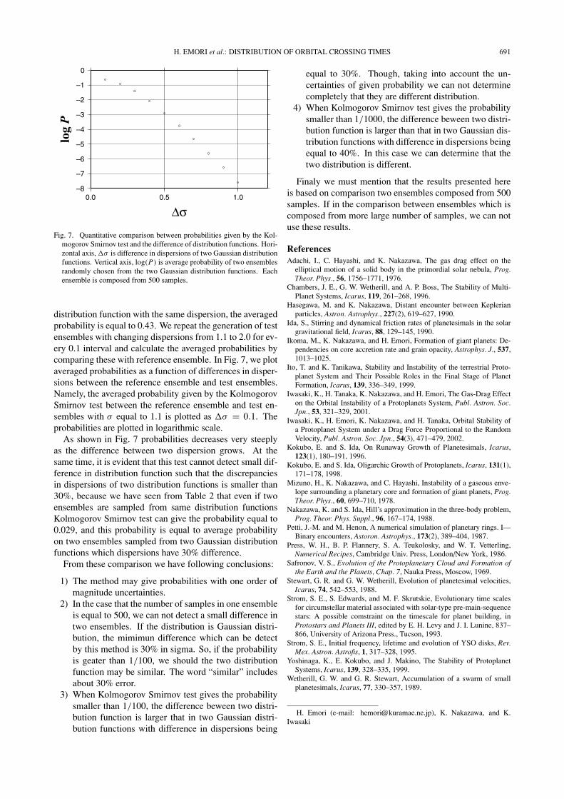
Fig. 7. Quantitative comparison between probabilities given by the Kol-mogorov Smirnov test and the difference of distribution functions. Hori-zontal axis, �σ is difference in dispersions of two Gaussian distributionfunctions. Vertical axis, log(P) is average probability of two ensemblesrandomly chosen from the two Gaussian distribution functions. Eachensemble is composed from 500 samples.

distribution function with the same dispersion, the averagedprobability is equal to 0.43. We repeat the generation of testensembles with changing dispersions from 1.1 to 2.0 for ev-ery 0.1 interval and calculate the averaged probabilities bycomparing these with reference ensemble. In Fig. 7, we plotaveraged probabilities as a function of differences in disper-sions between the reference ensemble and test ensembles.Namely, the averaged probability given by the KolmogorovSmirnov test between the reference ensemble and test en-sembles with σ equal to 1.1 is plotted as �σ = 0.1. Theprobabilities are plotted in logarithmic scale.

As shown in Fig. 7 probabilities decreases very steeplyas the difference between two dispersion grows. At thesame time, it is evident that this test cannot detect small dif-ference in distribution function such that the discrepanciesin dispersions of two distribution functions is smaller than30%, because we have seen from Table 2 that even if twoensembles are sampled from same distribution functionsKolmogorov Smirnov test can give the probability equal to0.029, and this probability is equal to average probabilityon two ensembles sampled from two Gaussian distributionfunctions which dispersions have 30% difference.

From these comparison we have following conclusions:

1) The method may give probabilities with one order ofmagnitude uncertainties.

2) In the case that the number of samples in one ensembleis equal to 500, we can not detect a small difference intwo ensembles. If the distribution is Gaussian distri-bution, the mimimun difference which can be detectby this method is 30% in sigma. So, if the probabilityis geater than 1/100, we should the two distributionfunction may be similar. The word “similar” includesabout 30% error.

3) When Kolmogorov Smirnov test gives the probabilitysmaller than 1/100, the difference beween two distri-bution function is larger that in two Gaussian distri-bution functions with difference in dispersions being

equal to 30%. Though, taking into account the un-certainties of given probability we can not determinecompletely that they are different distribution.

4) When Kolmogorov Smirnov test gives the probabilitysmaller than 1/1000, the difference beween two distri-bution function is larger than that in two Gaussian dis-tribution functions with difference in dispersions beingequal to 40%. In this case we can determine that thetwo distribution is different.

Finaly we must mention that the results presented hereis based on comparison two ensembles composed from 500samples. If in the comparison between ensembles which iscomposed from more large number of samples, we can notuse these results.

ReferencesAdachi, I., C. Hayashi, and K. Nakazawa, The gas drag effect on the

elliptical motion of a solid body in the primordial solar nebula, Prog.Theor. Phys., 56, 1756–1771, 1976.

Chambers, J. E., G. W. Wetherill, and A. P. Boss, The Stability of Multi-Planet Systems, Icarus, 119, 261–268, 1996.

Hasegawa, M. and K. Nakazawa, Distant encounter between Keplerianparticles, Astron. Astrophys., 227(2), 619–627, 1990.

Ida, S., Stirring and dynamical friction rates of planetesimals in the solargravitational field, Icarus, 88, 129–145, 1990.

Ikoma, M., K. Nakazawa, and H. Emori, Formation of giant planets: De-pendencies on core accretion rate and grain opacity, Astrophys. J., 537,1013–1025.

Ito, T. and K. Tanikawa, Stability and Instability of the terrestrial Proto-planet System and Their Possible Roles in the Final Stage of PlanetFormation, Icarus, 139, 336–349, 1999.

Iwasaki, K., H. Tanaka, K. Nakazawa, and H. Emori, The Gas-Drag Effecton the Orbital Instability of a Protoplanets System, Publ. Astron. Soc.Jpn., 53, 321–329, 2001.

Iwasaki, K., H. Emori, K. Nakazawa, and H. Tanaka, Orbital Stability ofa Protoplanet System under a Drag Force Proportional to the RandomVelocity, Publ. Astron. Soc. Jpn., 54(3), 471–479, 2002.

Kokubo, E. and S. Ida, On Runaway Growth of Planetesimals, Icarus,123(1), 180–191, 1996.

Kokubo, E. and S. Ida, Oligarchic Growth of Protoplanets, Icarus, 131(1),171–178, 1998.

Mizuno, H., K. Nakazawa, and C. Hayashi, Instability of a gaseous enve-lope surrounding a planetary core and formation of giant planets, Prog.Theor. Phys., 60, 699–710, 1978.

Nakazawa, K. and S. Ida, Hill’s approximation in the three-body problem,Prog. Theor. Phys. Suppl., 96, 167–174, 1988.

Petti, J.-M. and M. Henon, A numerical simulation of planetary rings. I—Binary encounters, Astoron. Astrophys., 173(2), 389–404, 1987.

Press, W. H., B. P. Flannery, S. A. Teukolosky, and W. T. Vetterling,Numerical Recipes, Cambridge Univ. Press, London/New York, 1986.

Safronov, V. S., Evolution of the Protoplanetary Cloud and Formation ofthe Earth and the Planets, Chap. 7, Nauka Press, Moscow, 1969.

Stewart, G. R. and G. W. Wetherill, Evolution of planetesimal velocities,Icarus, 74, 542–553, 1988.

Strom, S. E., S. Edwards, and M. F. Skrutskie, Evolutionary time scalesfor circumstellar material associated with solar-type pre-main-sequencestars: A possible comstraint on the timescale for planet building, inProtostars and Planets III, edited by E. H. Levy and J. I. Lunine, 837–866, University of Arizona Press., Tucson, 1993.

Strom, S. E., Initial frequency, lifetime and evolution of YSO disks, Rev.Mex. Astron. Astrofis, 1, 317–328, 1995.

Yoshinaga, K., E. Kokubo, and J. Makino, The Stability of ProtoplanetSystems, Icarus, 139, 328–335, 1999.

Wetherill, G. W. and G. R. Stewart, Accumulation of a swarm of smallplanetesimals, Icarus, 77, 330–357, 1989.

H. Emori (e-mail: [email protected]), K. Nakazawa, and K.Iwasaki

Documents

Probability distribution of orbital crossing times in a protoplanetary system