Embed Size (px)
Citation preview

Applied Statistics: Probability 1-1
Probability for Computer Scientists
This material is provided for the educational use of students in CSE2400 at FIT. No further use or reproduction is permitted.
Copyright G.A.Marin, 2008,All rights reserved.
Applied Statistics: Probability 1-2
Motivation: Here are some things I’ve done with prob/stat in my career:
Helped Texaco analyze seismic data to find new oil reserves.Helped Texaco analyze the bidding process for offshore oil leases.Helped US Navy search for submarines and develop ASW tactics.Helped US Navy evaluate capabilities of future forces.Helped IBM analyze performance of computer networks in health, airline reservation, banking, and other industries. Evaluated new networking technologies such as IBM’s Token Ring, ATM, Frame Relay…Analyzed meteor burst communications for US government (and weather and earthquakes...)
Applied Statistics: Probability 1-3
Motivation:I never could have imagined the opportunities I would have to use this material when I took a course like this one. You can’t either. Mostly I cannot teach about all of these problem areas because you must “master” the basics (this course) first. It is the key.This takes steady work. Have in mind about 6-8 hours per week (beginning this week!).
20 hours after 3 weeks is nowhere as good.If you begin now and learn as you go, you’ll likely succeed. If you don’t do anything, say, until the night before a test or the day before an assignment is due, you will not be likely to succeed.Now is the time to commit.

Applied Statistics: Probability 1-4
Suggestions on how to studyDo NOT bring a computer to class. It distracts you. Watch, listen and take notes the old fashioned way (pencil and paper). For example, write: slide 7 geom series?? Writing notes/questions actually helps you pay attention.As soon after class as possible review the slides covered in class and your class notes. Do not go to the “next” slide until you understand everything on the current slide.
Can’t understand something? Ask next class period or come to my office hours. In the words of Jerry McGuire: “Help me to help you.”Answer all points you raised in your notes. Look things up on the web.
Read the material in the text that corresponds to the slides covered. The syllabus gives you a good indication of where to look. Work a few homework problems each night (when homework is assigned).
Can’t work one or two of these problems? Come to my office hours. “Help me to help you.” It is much, much worse to come two days before 15 problems are due and say “I can’t do any of these.” I will help you with some of the work, but it’s like trying to learn a musical instrument just by watching me play it.)
Applied Statistics: Probability 1-5
Introduction to MathcadMathcad is computational software by Mathsoft Engineering and Education, Inc. It includes a computational engine, a word processor, and graphing tools. You enter equations “almost” as you would write them on paper. They evaluate “instantly.” You MUST use Mathcad for all homework in this class. Send your mathcad worksheet to [email protected] BEFORE class time on the due date. “I could not get a Mathcad terminal” is NO EXCUSE.
Name the worksheet HomeworknFirstnameLastname.xmcdThe letter n represents the number of the assignment. The “type” .xmcd is assigned automatically.If you do not follow the instructions, you will receive a zero for the homework assignment.
Mathcad is available (at no charge) in Olin EC 272.Tutorial and help are included with the software; resources are also available at mathcad.com. Mathcad OVERVIEW is next. Note: Homework 1 is on the web site.
Applied Statistics: Probability 1-6
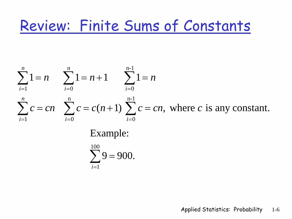
Review: Finite Sums of Constants
n n-1
1 0 0n n-1
1 0 0
1 1 1 1
( 1) , where is any constant.
n
i i in
i i i
n n n
c cn c c n c cn c
= = =
= = =
= = + =
= = + =
∑ ∑ ∑
∑ ∑ ∑
100
1
Example:
9 900.i=
=∑
Applied Statistics: Probability 1-7
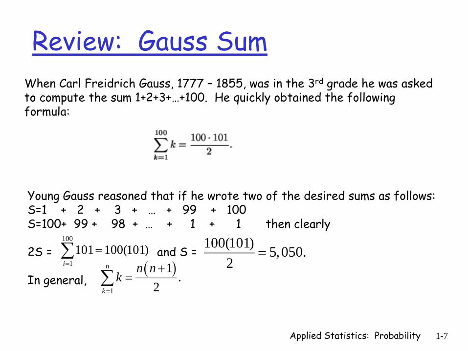
Review: Gauss SumWhen Carl Freidrich Gauss, 1777 – 1855, was in the 3rd grade he was asked to compute the sum 1+2+3+…+100. He quickly obtained the following formula:
Young Gauss reasoned that if he wrote two of the desired sums as follows:S=1 + 2 + 3 + … + 99 + 100S=100+ 99 + 98 + … + 1 + 1 then clearly
2S = and S =
In general,
100
1101 100(101)
i==∑ 100(101) 5,050.
2=
( )1
1.
2
n
k
n nk
=
+=∑
Applied Statistics: Probability 1-8
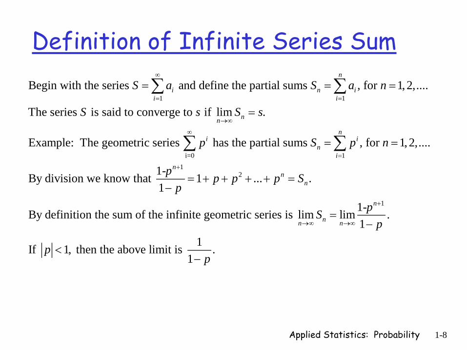
Definition of Infinite Series Sum
1 1
i=0
Begin with the series and define the partial sums , for 1, 2,....
The series is said to converge to if lim .
Example: The geometric series has the partial sums
n
i n ii i
nn
in
S a S a n
S s S s
p S
∞
= =
→∞
∞
= = =
=
∑ ∑
∑1
12
1
, for 1,2,....
1-By division we know that 1 ... .1
1-By definition the sum of the infinite geometric series is lim lim .1
1If 1, then the above limit is .1
ni
i
nn
n
n
nn n
p n
p p p p Sp
pSp
pp
=
+
+
→∞ →∞
= =
= + + + + =−
=−
<−
∑
Applied Statistics: Probability 1-9
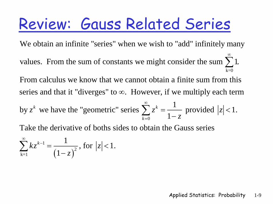
Review: Gauss Related Series
k=0
We obtain an infinite "series" when we wish to "add" infinitely many
values. From the sum of constants we might consider the sum 1.
From calculus we know that we cannot obtain a finite sum from t
∞
∑
0
k=
hisseries and that it "diverges" to . However, if we multiply each term
1by we have the "geometric" series provided 1.1
Take the derivative of boths sides to obtain the Gauss series
k k
kz z z
z
k
∞
=
∞
= <−∑
( )1
21
1 , for 1.1
kz zz
∞− = <
−∑
Applied Statistics: Probability 1-10
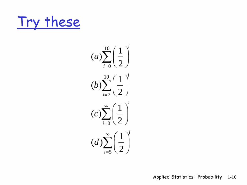
Try these10
0
10
2
0
5
1( )2
1( )2
1( )2
1( )2
i
i
i
i
i
i
i
i
a
b
c
d
=
=
∞
=
∞
=
⎛ ⎞⎜ ⎟⎝ ⎠
⎛ ⎞⎜ ⎟⎝ ⎠
⎛ ⎞⎜ ⎟⎝ ⎠
⎛ ⎞⎜ ⎟⎝ ⎠
∑
∑
∑
∑
Applied Statistics: Probability 1-11
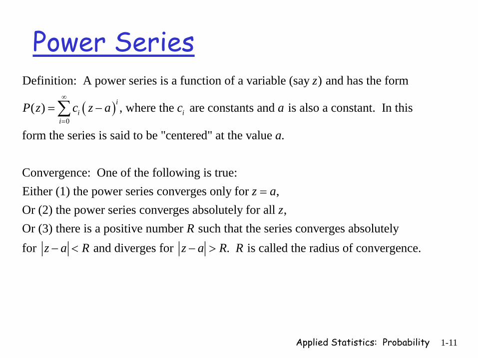
Power Series
( )0
Definition: A power series is a function of a variable (say ) and has the form
( ) , where the are constants and is also a constant. In this
form the series is said to be "centered"
ii i
i
z
P z c z a c a∞
=
= −∑at the value .
Convergence: One of the following is true:Either (1) the power series converges only for ,Or (2) the power series converges absolutely for all ,Or (3) there is a positive number
a
z az
R
=
such that the series converges absolutelyfor and diverges for . is called the radius of convergence.z a R z a R R− < − >

Applied Statistics: Probability 1-12
Ratio Test (Good tool for finding radius of convergence.)
1
k=0Consider the series and suppose that lim 0 (or infinite).
If <1, then the series converges absolutely. If >1 or , the seriesdiverges.
kk k
k
aa
aρ
ρ ρ ρ
∞+
→∞= >
= ∞
∑
1
1
1Example: Determine where the series converges. 3
11 3
The ratio . The limit lim ;1 3 1 3 31
3
thus, . It follows that the series c3
k
k
k
kk k
k
xk
xka k x k x x
a k kxk
xρ
∞
=
+
→∞
⎛ ⎞⎛ ⎞⎜ ⎟⎜ ⎟⎝ ⎠⎝ ⎠
⎛ ⎞⎛ ⎞⎜ ⎟⎜ ⎟+⎝ ⎠⎝ ⎠
= = =+ +⎛ ⎞⎛ ⎞
⎜ ⎟⎜ ⎟⎝ ⎠⎝ ⎠
=
∑
onverges for 1 3, and3
the series diverges for 3.
x x
x
< ⇒ <
>
Color red means – not on test!

Applied Statistics: Probability 1-13
Review: Other Useful Series
Exponential function:
The sum of squares:
Binomial sum:
Geometric sum:1
0
11
nnk
k
zzz
+
=
−=
−∑
Applied Statistics: Probability 1-14
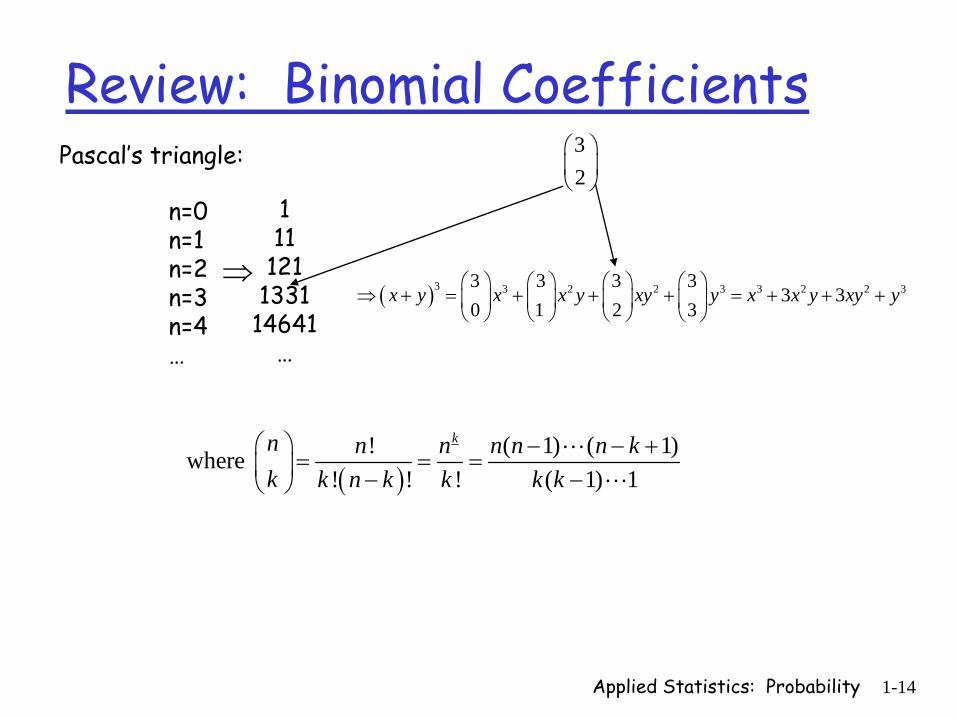
Review: Binomial Coefficients
111
1211331
14641…
Pascal’s triangle:
n=0n=1n=2n=3n=4…
⇒
( )! ( 1) ( 1)where
! ! ! ( 1) 1
kn n n n n n kk k n k k k k
⎛ ⎞ − − += = =⎜ ⎟ − −⎝ ⎠
32
⎛ ⎞⎜ ⎟⎝ ⎠
( )3 3 2 2 3 3 2 2 33 3 3 33 3
0 1 2 3x y x x y xy y x x y xy y⎛ ⎞ ⎛ ⎞ ⎛ ⎞ ⎛ ⎞
⇒ + = + + + = + + +⎜ ⎟ ⎜ ⎟ ⎜ ⎟ ⎜ ⎟⎝ ⎠ ⎝ ⎠ ⎝ ⎠ ⎝ ⎠

Applied Statistics: Probability 1-15
Floors and CeilingsAs usual we define the greatest integer less than or equal to where is any real number. Similarly we define the smallest integer greater than or equal to .
Thus, 2.3 2
x x x
x x
=⎢ ⎥⎣ ⎦
=⎡ ⎤⎢ ⎥
=⎢ ⎥⎣ ⎦ while 2.3 3.
Also, -7.6 8 while -7.6 7.
Only when is an integer do we have equality of these functions: .
In fact, when is not an integer, then 1.
xx x x
x x x
=⎡ ⎤⎢ ⎥= − = −⎢ ⎥ ⎡ ⎤⎣ ⎦ ⎢ ⎥
= =⎢ ⎥ ⎡ ⎤⎣ ⎦ ⎢ ⎥− =⎡ ⎤ ⎢ ⎥⎢ ⎥ ⎣ ⎦
Applied Statistics: Probability 1-16
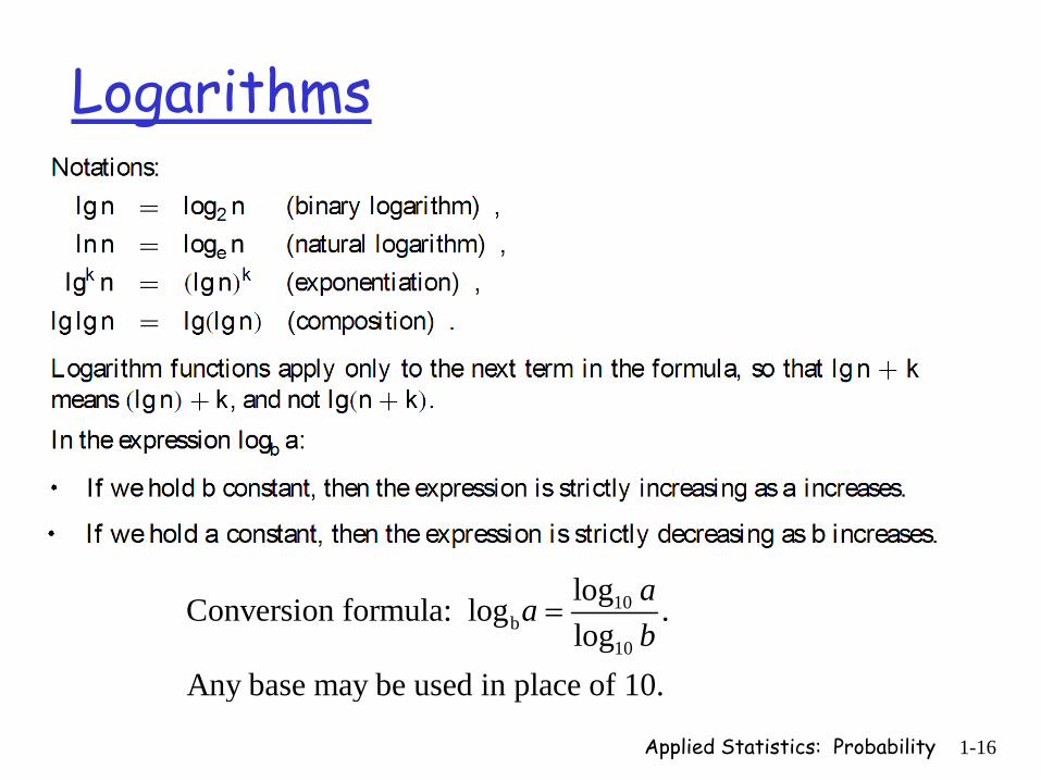
Logarithms
10b
10
logConversion formula: log .log
Any base may be used in place of 10.
aab
=
Applied Statistics: Probability 1-17
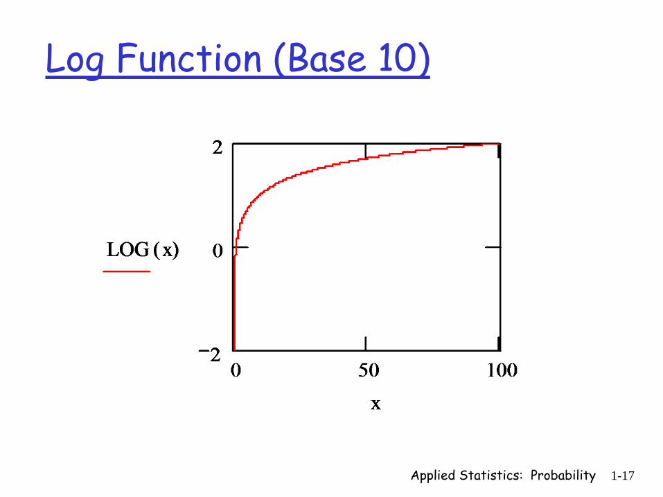
Log Function (Base 10)
Applied Statistics: Probability 1-18
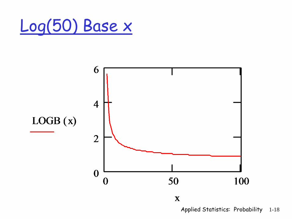
Log(50) Base x

Applied Statistics: Probability 1-19
Logarithmic Identities

Applied Statistics: Probability 1-20
Notation, notation, notationLearning math in many ways is like learning a new language. You may understand a concept but be unable to write it down. You may not be able to read notation that represents a simple concept. The only way to tackle this “language barrier” is through repetition until the notation begins to look “friendly.” You must try writing results yourself (begin with blank paper) until you can recall the notation that expresses the concepts.
Copy theorems from class or from the text until you can rewrite them without looking at the material and you understand what you are writing.
Probability and statistics introduce their own notation to be mastered. If you begin tonight, and spend time after every class, you can learn this new language. If you wait until the week before the test, it will be much like trying to learn Spanish, or French, or English in just a few nights (1 night??). It really can’t be done.

Applied Statistics: Probability 1-21
Math sentencesMath problems, theorem, solutions ... must be written in sentences that makesense when you read them (EVEN WHEN EQUATIONS ARE USED). Youwill notice that I am careful to do this to the greatest extent possible on theseslides (even knowning that I will explain them in class).
My observation is that most students have no idea how to do this. I often seesolutions like the following on homework or t
42
02
3
est papers:
Evaluate . The student writes something like
364 .3
x dx
xx
=
=
=
∫The answer is right BUT every step is nonsense. The = sign means “is equal to.” In the first step, we don’t know to what the equality refers. The equality is simply wrong in the next two steps.
44 32
0 0
Instead write:
64 640 .3 3 3xx dx = = − =∫
Applied Statistics: Probability 1-22
Permutations and Combinations1 2Suppose that we have objects , ,..., .
A permutation of order is an "ordered" selection of of these for 1 n.A combination of order is an "unordered" selection of of these. Com
nn O O O
k k kk k
≤ ≤
( )
( )
mon notation: , or ( 1) ( 1)
, .!
Example: Given the 5 letters a,b,c,d,e how many ways can we list 3 of the 5when order is
n kk
knk
P n k P n n n k n
n nC n k Ck k
= − − + =
⎛ ⎞= = =⎜ ⎟
⎝ ⎠
5 33
important?Answer: =5 =5*4*3=60.Note that each choice of 3 letters (such as a,c,e) results in 6 different results:ace, aec, cae, cea, eac, eca... Example: Given the 5 letters above how ma
P
3
ny ways can we choose 3 of the 5when order is NOT important?
5 5 5*4*3Answer: = = 10. In this case we have the 60 that result when we care about order3 3! 3*2*1
divided by 6 (the number of orderi
⎛ ⎞=⎜ ⎟
⎝ ⎠ngs of 3 fixed letters).
Applied Statistics: Probability 1-23
Definition
3
6
( 1) ( 1) for any positive integer and for integers such that 1 . This symbol is pronouced " to the falling."
Examples: 6 6 5 4 120. 3 is not defined (for our
kn n n n k n kk n n k
= × − × × − +≤ ≤
= × × =
5
purposes). 5 5!
Again: and .!
kn k
k
n nP nk k
=
⎛ ⎞= =⎜ ⎟
⎝ ⎠
Applied Statistics: Probability 1-24
Permutations of Multiple Types
1 2 1
2
1 2
The number of permutations of objects of which are ofone type, are of a second type, ..., and are of an type is
! .! ! !
r
r
r
n n n n nn n rth
nn n n
= + + +
Example: Suppose we have 2 red buttons, 3 white buttons, and 4 blue buttons.How many different orderings (permutations) are there?
9!Answer: 1260.2!3!4!
=
Applied Statistics: Probability 1-25
Try TheseThere are 12 marbles in an urn. 8 are white and 4 are red. The white marblesare numbered w1,w2,...,w8 and the red ones are numbered r1,r2,r3,r4. For (a) - (d): Without looking into the urn you dra
5
w out 5 marbles. (a) How many unique choices can you get if order matters? 12 95,040
12(b) How many unique choices can you get if order does not matter? 792
5(c) How many ways can you choose 3
=
⎛ ⎞=⎜ ⎟
⎝ ⎠ white marbles and 2 red marbles if
order matters? You will fill 5 "slots" by drawing. First determine which5
two slots (positions) will be occupied by 2 red marbles: 10. Next2
⎛ ⎞=⎜ ⎟
⎝ ⎠3 2multiply by orderings of 3 white and 2 red: 10 8 4 40,320.
(d) How many ways can you choose 3 white marbles and 2 red marbles if8 4
order does not matter? 3363 2
(e) How many marbles
=
⎛ ⎞⎛ ⎞=⎜ ⎟⎜ ⎟
⎝ ⎠⎝ ⎠
i i
must you draw to be sure of getting two red ones? 10

Applied Statistics: Probability 1-26
Complex CombinationsHow many ways are there to create a “full house” (3-of-a-kind plus a pair) using a standard deck of 52 playing cards?
13 4 12 413 4 12 6 3,744.
1 3 1 2⎛ ⎞⎛ ⎞⎛ ⎞⎛ ⎞
= =⎜ ⎟⎜ ⎟⎜ ⎟⎜ ⎟⎝ ⎠⎝ ⎠⎝ ⎠⎝ ⎠
i i i
(choose denomination)x(choose 3 of 4 of given denomination)x(choose one of the remaining denominations)x(choose 2 of 4 of this second denomination).
This follows from the multiplication principle (Theorem 2.3.1 in text).

Applied Statistics: Probability 1-27
Try these…
Suppose . What is ?11 7
18 18Suppose . What is ?
2
n nn
rr r
⎛ ⎞ ⎛ ⎞=⎜ ⎟ ⎜ ⎟
⎝ ⎠ ⎝ ⎠⎛ ⎞ ⎛ ⎞
=⎜ ⎟ ⎜ ⎟−⎝ ⎠ ⎝ ⎠
Applied Statistics: Probability 1-28
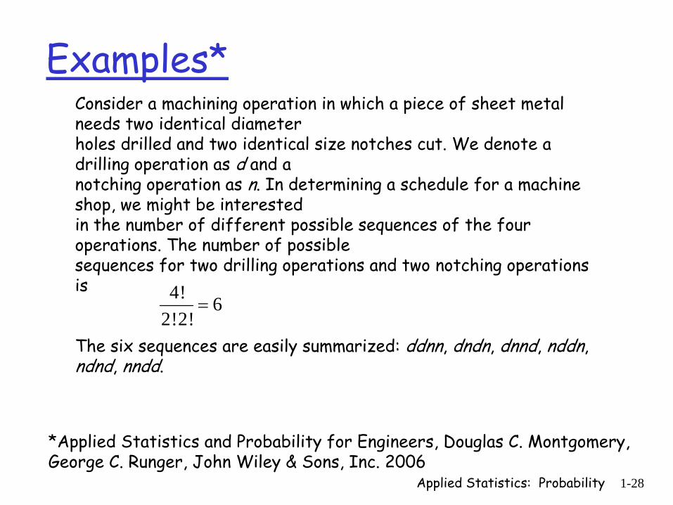
Examples*Consider a machining operation in which a piece of sheet metal needs two identical diameterholes drilled and two identical size notches cut. We denote a drilling operation as d and anotching operation as n. In determining a schedule for a machine shop, we might be interestedin the number of different possible sequences of the four operations. The number of possiblesequences for two drilling operations and two notching operations is
The six sequences are easily summarized: ddnn, dndn, dnnd, nddn, ndnd, nndd.
*Applied Statistics and Probability for Engineers, Douglas C. Montgomery,George C. Runger, John Wiley & Sons, Inc. 2006
4! 62!2!
=
Applied Statistics: Probability 1-29
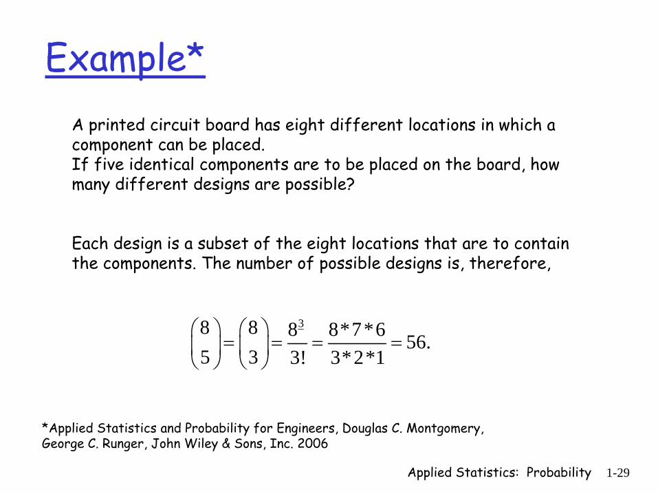
Example*A printed circuit board has eight different locations in which a component can be placed. If five identical components are to be placed on the board, how many different designs are possible?
Each design is a subset of the eight locations that are to contain the components. The number of possible designs is, therefore,
38 8 8 8*7*6 56.5 3 3! 3*2*1
⎛ ⎞ ⎛ ⎞= = = =⎜ ⎟ ⎜ ⎟
⎝ ⎠ ⎝ ⎠
*Applied Statistics and Probability for Engineers, Douglas C. Montgomery,George C. Runger, John Wiley & Sons, Inc. 2006

Applied Statistics: Probability 1-30
Sample SpaceDefinition: The totality of the possible outcomes of a random experiment is called the Sample Space,
Finite
Countable
Continuous (We begin with the discrete cases.)
.Ω
{ }Outcome from one roll of one die 1, 2,3, 4,5,6 .⇒ Ω =
{ }
The number of attempts until a message is transmitted successfullywhen the probability of success on any one attempt is 1, 2,3, 4,5,6,... .
p+⇒ Ω = =
{ }The time (in seconds) until a lightbulb burns out
: 0 , where is the set of all real numbers.t t⇒ Ω = ∈ ≥
Applied Statistics: Probability 1-31
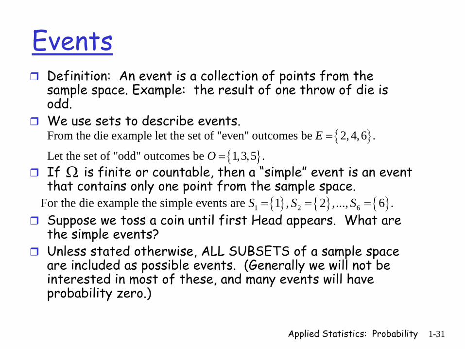
EventsDefinition: An event is a collection of points from the sample space. Example: the result of one throw of die is odd.We use sets to describe events.
If is finite or countable, then a “simple” event is an event that contains only one point from the sample space.
Suppose we toss a coin until first Head appears. What are the simple events?Unless stated otherwise, ALL SUBSETS of a sample space are included as possible events. (Generally we will not be interested in most of these, and many events will have probability zero.)
{ }{ }
From the die example let the set of "even" outcomes be 2, 4,6 .
Let the set of "odd" outcomes be 1,3,5 .
E
O
=
=Ω
{ } { } { }1 2 6For the die example the simple events are 1 , 2 ,..., 6 .S S S= = =
Applied Statistics: Probability 1-32
Describe the sample space and events
Each of 3 machine parts is classified as either above or below spec.
At least one part is below spec.An order for an automobile can specify either an automatic or standard transmission, premium or standard stereo, V6 or V8 engine, leather or cloth interior, and colors: red, blue, black, green, white.
Orders have premium stereo, leather interior, and a V8 engine.
Applied Statistics: Probability 1-33
Describe: sample space and eventsThe number of hours of normal use of a lightbulb.
Lightbulbs that last between 1500 and 1800 hours.The individual weights of automobiles crossing a bridge measured in tons to nearest hundredth of a ton.
Autos crossing that weigh more than 3,000 pounds.A message is transmitted repeatedly until transmission is successful.
Those messages transmitted 3 or fewer times.

Applied Statistics: Probability 1-34
Operations on Events
Both and occur. At least one of or occurs.
does not occur.
occurs and does not occur. the empty set (a set that contains no elements).
and are "mutually exclus
A B A BA B A B
A A
S A S A S A
A B A B
∩ ⇒∪ ⇒
⇒
∩ = − ⇒∅ ⇒
∩ = ∅ ⇒ ive."Every element of is an element of , or, if occurs, occurs.
Review Venn diagrams (in text).
A B A B A B⊂ ⇒
Because the sample space is a set, , and any event is a subset , weform new events from existing events by using the usual set theory operations.
AΩ ⊂ Ω
Applied Statistics: Probability 1-35
ExampleFour bits are transmitted over a digital communications channel. Each bit iseither distorted or received without distortion. Let denote the event thatthe th bit is distorted, 1, 2,3,4.(a) Desc
iAi i =
1
1 2
1 2
1
ribe the sample space.
(b) What is the event ?
(c) What is the event ?
(c) What is the event ?
(d) What is the event ?
A
A A
A A
A
∪
∩
′

Applied Statistics: Probability 1-36
Venn Diagrams Identify the following events:
A B
C
( )
( )
( ) ( ) ( ) ( )
( )
(e)
a Ab A Bc A B C
d B C
A B C
′
∩∩ ∪
′∪
′∩ ∪
Applied Statistics: Probability 1-37
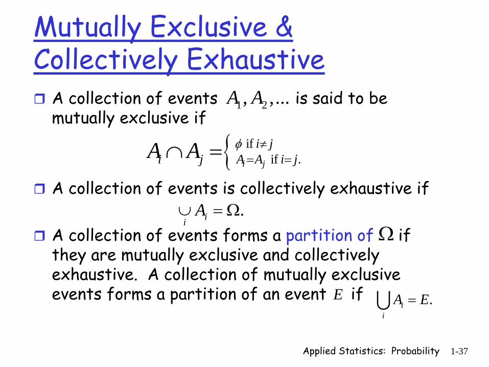
Mutually Exclusive & Collectively Exhaustive
A collection of events is said to be mutually exclusive if
A collection of events is collectively exhaustive if
A collection of events forms a partition of if they are mutually exclusive and collectively exhaustive. A collection of mutually exclusive events forms a partition of an event if
1 2, ,...A A
{ if if .i j
i ji j A A i jA A φ ≠
= =∩ =
.iiA∪ = Ω
Ω
E .ii
A E=∪
Applied Statistics: Probability 1-38
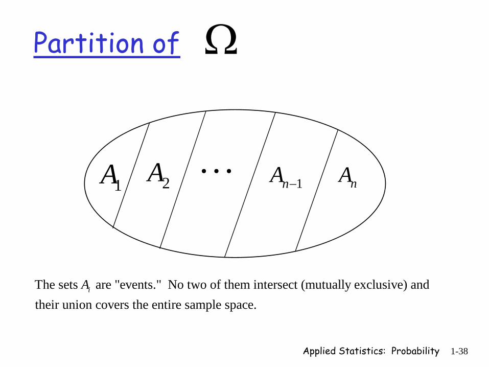
Partition of Ω
1A 2A 1nA − nA
The sets are "events." No two of them intersect (mutually exclusive) and their union covers the entire sample space.
iA

Applied Statistics: Probability 1-39
Probability measureWe use a probability measure to represent the relative likelihood that a random event will occur. The probability of an event is denoted
Axioms:( ).P A
A
1 2
1
A1. For every event , ( ) 0.A 2. ( ) 1.A3. If and are m utually exclusive, then P(A B)=P(A)+P(B).A4. If the events , , ... are m utually exclusive, then
( )n nnn
A P AP
A B
A A
P A P A∞
==
≥Ω =
∪
⎡ ⎤=⎢ ⎥
⎣ ⎦∪
1
.∞
∑

Applied Statistics: Probability 1-40
Theorem:
( )[ ][ ] [ ] [ ] [ ]
Given a sample space, , a "well-defined" collection of events,, and a probability measure, , defined on these events then
the following hold:
(a) 0.
(b) 1 , .
(c) , ,
P
P
P A P A A
P A B P A P B P A B A
Ω
∅ =
⎡ ⎤= − ∀ ∈⎣ ⎦∪ = + − ∩ ∀
F
F
[ ] [ ].
(d) , , .
B
A B P A P B A B
∈
⊂ ⇒ ≤ ∀ ∈
FF
You must “know” these and be able to use them to solve problems. Don’t worry about proving them.
Applied Statistics: Probability 1-41
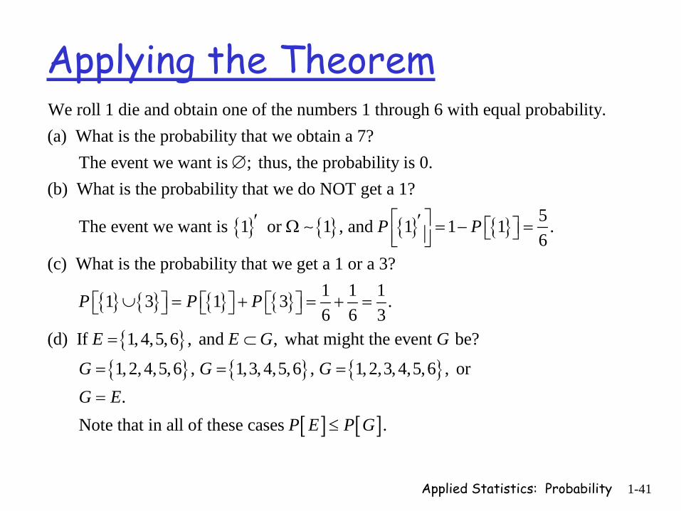
Applying the TheoremWe roll 1 die and obtain one of the numbers 1 through 6 with equal probability. (a) What is the probability that we obtain a 7? The event we want is ; thus, the probability is 0.(b) What is t
∅
{ } { } { } { }
{ } { } { } { }
he probability that we do NOT get a 1?5 The event we want is 1 or 1 , and 1 1 1 .6
(c) What is the probability that we get a 1 or a 3?1 1 1 1 3 1 3 .6 6 3
(d) I
P P
P P P
⎡ ⎤′ ′Ω = − =⎡ ⎤⎣ ⎦⎢ ⎥⎣ ⎦
∪ = + = + =⎡ ⎤ ⎡ ⎤ ⎡ ⎤⎣ ⎦ ⎣ ⎦ ⎣ ⎦
∼
{ }{ } { } { }
[ ] [ ]
f 1, 4,5,6 , and , what might the event be?
1, 2,4,5,6 , 1,3, 4,5,6 , 1, 2,3,4,5,6 , or . Note that in all of these cases .
E E G G
G G GG E
P E P G
= ⊂
= = =
=
≤
Applied Statistics: Probability 1-42
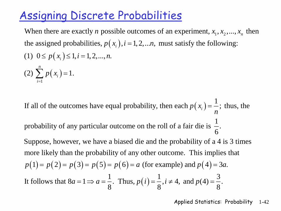
Assigning Discrete Probabilities
( )( )
( )
1 2
1
When there are exactly possible outcomes of an experiment, , ,..., thenthe assigned probabilities, , 1, 2,... , must satisfy the following:
(1) 0 1, 1, 2,..., .
(2) 1.
If all of t
n
i
i
n
ii
n x x xp x i n
p x i n
p x=
=
≤ ≤ =
=∑
( ) 1he outcomes have equal probability, then each ; thus, the
1probability of any particular outcome on the roll of a fair die is .6
Suppose, however, we have a biased die and the probability of a 4
ip xn
=
( ) ( ) ( ) ( ) ( ) ( )
( )
is 3 timesmore likely than the probability of any other outcome. This implies that
1 2 3 5 6 (for example) and 4 3 .1 1 3It follows that 8 1 . Thus, , 4, and (4) .8 8 8
p p p p p a p a
a a p i i p
= = = = = =
= ⇒ = = ≠ =
Applied Statistics: Probability 1-43
Exercises:Suppose Bigg Fakir claims that by clairvoyance he can tell the numbers of four cards numbered 1 to 4 that are laid face down on a table. (He must chooseall 4 cards before turning any over.) If he has no special powers and guesses at random, calculate the following:(a) the probability that Bigg gets at least one right(b) the probability he gets two right(c) the probability Bigg gets them all right. Note: assume that Bigg must guess the value of each card before looking at any of the cards.
Hint: What is the sample space? How are the probabilities assigned?
Applied Statistics: Probability 1-44
Bigg Fakir Solution
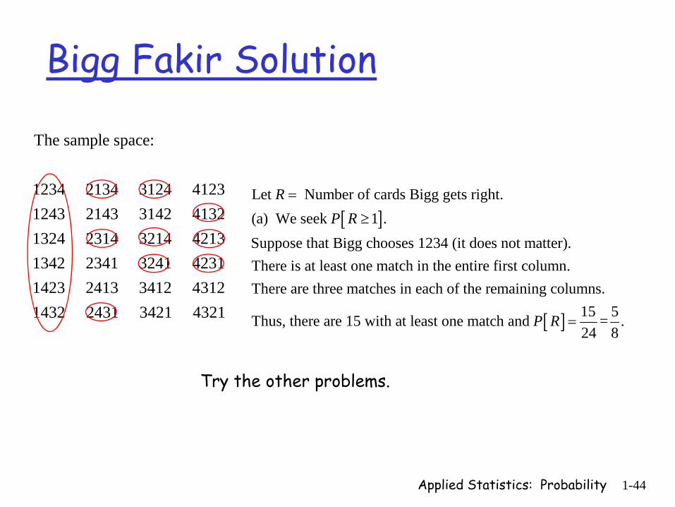
The sample space:
1234 2134 3124 41231243 2143 3142 41321324 2314 3214 42131342 2341 3241 42311423 2413 3412 43121432 2431 3421 4321
[ ]Let Number of cards Bigg gets right. (a) We seek 1 .Suppose that Bigg chooses 1234 (it does not matter).There is at least one match in the entire first column.There are three matches in each of
RP R
=
≥
[ ]
the remaining columns.15 5Thus, there are 15 with at least one match and = . 24 8
P R =
Try the other problems.

Applied Statistics: Probability 1-45
Complex CombinationsHow many ways are there to create a “full house” (3-of-a-kind plus a pair) using a standard deck of 52 playing cards?
13 4 12 413 4 12 6 3,744.
1 3 1 2⎛ ⎞⎛ ⎞⎛ ⎞⎛ ⎞
= =⎜ ⎟⎜ ⎟⎜ ⎟⎜ ⎟⎝ ⎠⎝ ⎠⎝ ⎠⎝ ⎠
i i i
(choose denomination)x(choose 3 of 4 of given denomination)x(choose one of the remaining denominations)x(choose 2 of 4 of this second denomination).
This follows from the multiplication principle (Theorem 2.3.1 in text).

Applied Statistics: Probability 1-46
What is the probability of a “full house”?In discrete problems we interpret probability as a ratio:
number of successful outcomes .total number of outcomes.
In this case the number of successful outcomes is
successessuccesses failures
=+
5
the numberof ways to get a full house (3,744). The total number of outcomes is:
52 52 52 51 50 49 48 2,598,960.5 5! 5 4 3 2 1
3,744Thus, the probability of getting a full house is 2,59
⎛ ⎞= = =⎜ ⎟
⎝ ⎠
i i i ii i i i
0.001448,960
This is an example of a hypergeometric distribution; we'll study this soon.
=
A full house happens about once in every 694 hands! This is why people invented wild cards.
Applied Statistics: Probability 1-47
Conditional Probability
The conditional probability of given that has occurred is
Q1: What is the probability of obtaining a total of 8 when rolling two dice?Q2: Suppose you roll two dice that you cannot see. Someone tells you that the sum is greater than 6. What is the probability that the sum is 8?
AB
( )( )( | ) , provided 0.( )
P A BP A B P BP B
∩= ≠

Applied Statistics: Probability 1-48
Dice Problem
( )( )( )( )
Let be the event of getting 8 on the roll of two dice. Let be the event that the sum of the two dice is greater than 6. The first question is Find ( ).Here is the sample space:
(1,1) 1,2 1,3 1,4 1,5
A BP A
( )( ) ( )( )( )( )( )( )( )( )( )( ) ( )( )( )( )( )( ) ( ) ( )( )( )( ) ( )( ) ( )
1,6
(2,1) 2,2 2,3 2,4 2,5 2,6
(3,1) 3,2 3,3 3, 4 3,5 3,6
(4,1) 4,2 4,3 4,4 4,5 4,6
(5,1) 5,2 5,3 5, 4 5,5 5,6
(6,1) 6,2 6,3 6,4 6,5 6,6
5( ) .36
P A =
Sum=8.
because we are assuming that each outcome pair has the same probability, 1/36.
Applied Statistics: Probability 1-49
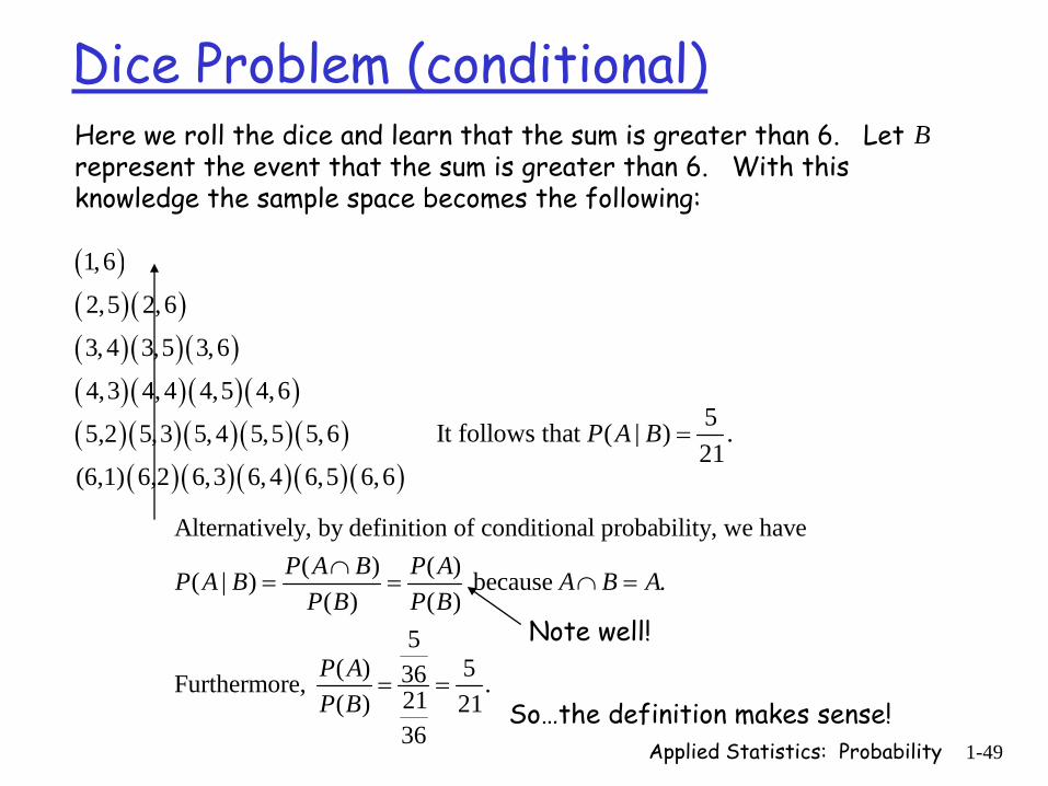
Dice Problem (conditional)Here we roll the dice and learn that the sum is greater than 6. Let represent the event that the sum is greater than 6. With this knowledge the sample space becomes the following:
( )( )( )( ) ( ) ( )( ) ( ) ( )( )( )( ) ( )( )( )
( )( )( ) ( )( )
1,6
2,5 2,6
3, 4 3,5 3,6
4,3 4, 4 4,5 4,6
5,2 5,3 5, 4 5,5 5,6
(6,1) 6,2 6,3 6, 4 6,5 6,6
5It follows that ( | ) .21
P A B =
Alternatively, by definition of conditional probability, we have( ) ( )( | ) because .
( ) ( )5
( ) 536Furthermore, .21( ) 2136
P A B P AP A B A B AP B P B
P AP B
∩= = ∩ =
= =So…the definition makes sense!
Note well!
B
Applied Statistics: Probability 1-50
Try this.
A university has 600 freshmen, 500 sophomores, and 400 juniors. 80 of the freshmen, 60 of the sophomores, and 50 of the juniors are Computer Science majors. For this problem assume there are NO seniors.
What is the probability that a student, selected at random, is a freshman or a CS major (or both)?
If a student is a CS major, what is the probability he/she is a sophomore?
Applied Statistics: Probability 1-51
Use these steps to solve previous slide
1. What is the sample space?2. What are the events (subsets) of
interest?3. What are the probabilities of the events
of interest?4. What is the answer to the problem?
Applied Statistics: Probability 1-52
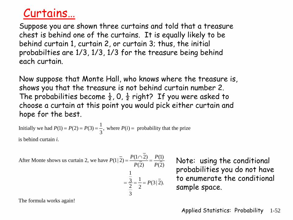
Curtains…Suppose you are shown three curtains and told that a treasure chest is behind one of the curtains. It is equally likely to be behind curtain 1, curtain 2, or curtain 3; thus, the initial probabilties are 1/3, 1/3, 1/3 for the treasure being behind each curtain.
Now suppose that Monte Hall, who knows where the treasure is, shows you that the treasure is not behind curtain number 2. The probabilities become ½, 0, ½ right? If you were asked to choose a curtain at this point you would pick either curtain and hope for the best.
1Initially we had (1) (2) (3) , where ( ) probability that the prize3
is behind curtain .
(1 2) (1)After Monte shows us curtain 2, we have (1| 2)(2) (2)
P P P P i
i
P PPP P
= = = =
∩= =
113 (3 | 2).2 2
3The formula works again!
P= = =
Note: using the conditional probabilities you do not have to enumerate the conditional sample space.

Applied Statistics: Probability 1-53
Curtains RevisitedWe change the game as follows. Again the treasure is hidden behind one ofthree curtains. At the beginning of the game you pick one of the curtains - say2. Then Monte shows you that the treasure is NOT behind curtain 3. Nowhe offers you a chance to switch your choice to curtain 1 or to stay with youroriginal choice of 2. Which should you do? Does the choice make a difference?
Applied Statistics: Probability 1-54
Here’s the deal…1 1 13 3 3
13
After you make your choice (but have not seen what's behind your curtain), the probabilities remain , , . Right? This means that the probability thatthe treasure is behind your curtain is and
23
the probability that it is behind one of the other curtains is . Monte will NEVER show you the treasure;thus, even after he shows you one of the curtains, the probability that the treasure is behi 2
3nd the curtain you did not choose is . It is twice as likely to be behind the other curtain so... you should always switch!
Moral of the story: be REALLY careful about underlying assumptionsabout the sample space and how it changes to create the conditional sample space. You are generally assuming the changes are random. Maybe they are not.
Applied Statistics: Probability 1-55
Alternate Form
( )( )( | ) , provided 0.( )
P A BP A B P BP B
∩= ≠
We have seen that the conditional probability of event given that event has occurred is:
AB
Clearly this implies that ( ) ( | ) ( ). This is referred to as the"multiplication rule," and holds even when ( ) 0. Notice that we could alsowrite ( ) ( | ) ( ). Both these equations alwa
P A B P A B P BP B
P A B P B A P A
∩ ==
∩ = ys hold for anytwo events. But there is a special case where the conditional probabilities aboveare not needed.
Note: memorize these conditional probability equations TODAY. They are extremely important.

Applied Statistics: Probability 1-56
Independent Events
Two events are independent iff the probability Example (dice)
Q1: If one die is rolled twice, is the probability of getting a 3 on the first roll independent of the probability of getting a 3 on the second roll? Q2: If one die is rolled twice, is the probability that their sum is greater than 5 independent of the probability that the first roll produces a 1?
and A B( ) ( ) ( ).PA B PAPB∩ =
Applied Statistics: Probability 1-57
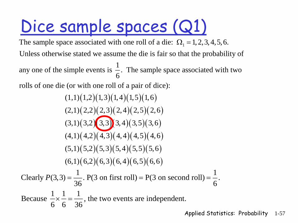
Dice sample spaces (Q1)1The sample space associated with one roll of a die: 1, 2,3, 4,5,6.
Unless otherwise stated we assume the die is fair so that the probability of1any one of the simple events is . The sample space as6
Ω =
( )( )( )( )( )( )( )( )( )( )( )( )( )
sociated with two
rolls of one die (or with one roll of a pair of dice): (1,1) 1,2 1,3 1,4 1,5 1,6
(2,1) 2,2 2,3 2, 4 2,5 2,6
(3,1) 3,2 3,3 3, 4 3,( )( )( )( )( )( )( )( )( )( )( )( )( )( )( )( )( )
5 3,6
(4,1) 4,2 4,3 4, 4 4,5 4,6
(5,1) 5,2 5,3 5,4 5,5 5,6
(6,1) 6,2 6,3 6,4 6,5 6,61 1Clearly (3,3) . P(3 on first roll) P(3 on second roll) .
36 61 1 1Because , the two events are independent. 6 6 36
P = = =
× =
Applied Statistics: Probability 1-58
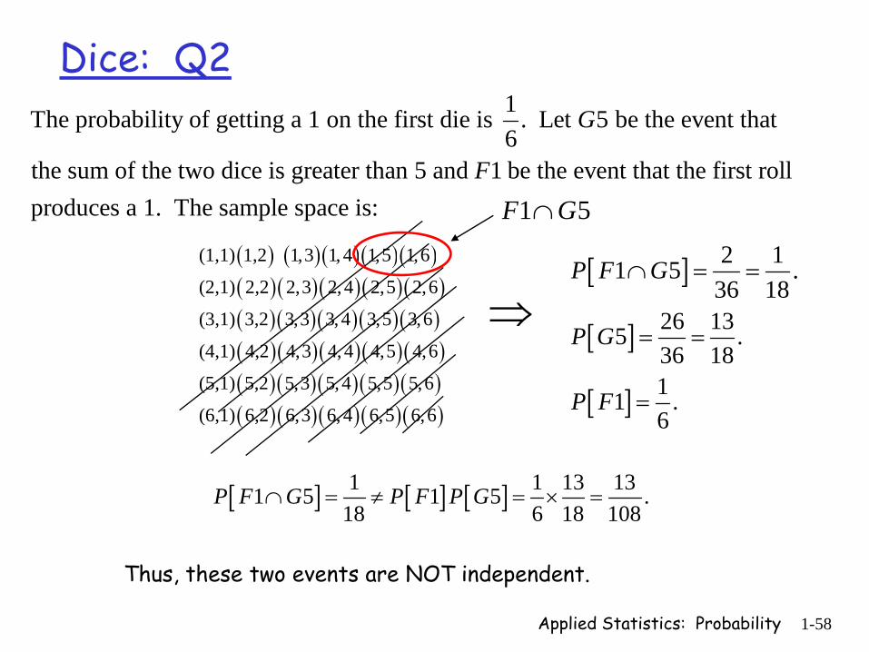
Dice: Q21The probability of getting a 1 on the first die is . Let 5 be the event that6
the sum of the two dice is greater than 5 and 1 be the event that the first rollproduces a 1. The sample space is:
G
F
( ) ( )( )( )( )( )( )( )( )( )( )( )( )( )( )( )( )( )( )( )
(1,1) 1,2 1,3 1, 4 1,5 1,6
(2,1) 2,2 2,3 2,4 2,5 2,6
(3,1) 3,2 3,3 3,4 3,5 3,6
(4,1) 4,2 4,3 4,4 4,5 4,6
( )( )( )( )( )( )( )( )( )( )
(5,1) 5,2 5,3 5,4 5,5 5,6
(6,1) 6,2 6,3 6, 4 6,5 6,6
[ ]
[ ]
26 135 .36 1811 .6
P G
P F
= =
=
⇒
1 5F G∩
[ ] 2 11 5 .36 18
P F G∩ = =
[ ] [ ] [ ]1 1 13 131 5 1 5 .18 6 18 108
P F G P F P G∩ = ≠ = × =
Thus, these two events are NOT independent.
Applied Statistics: Probability 1-59
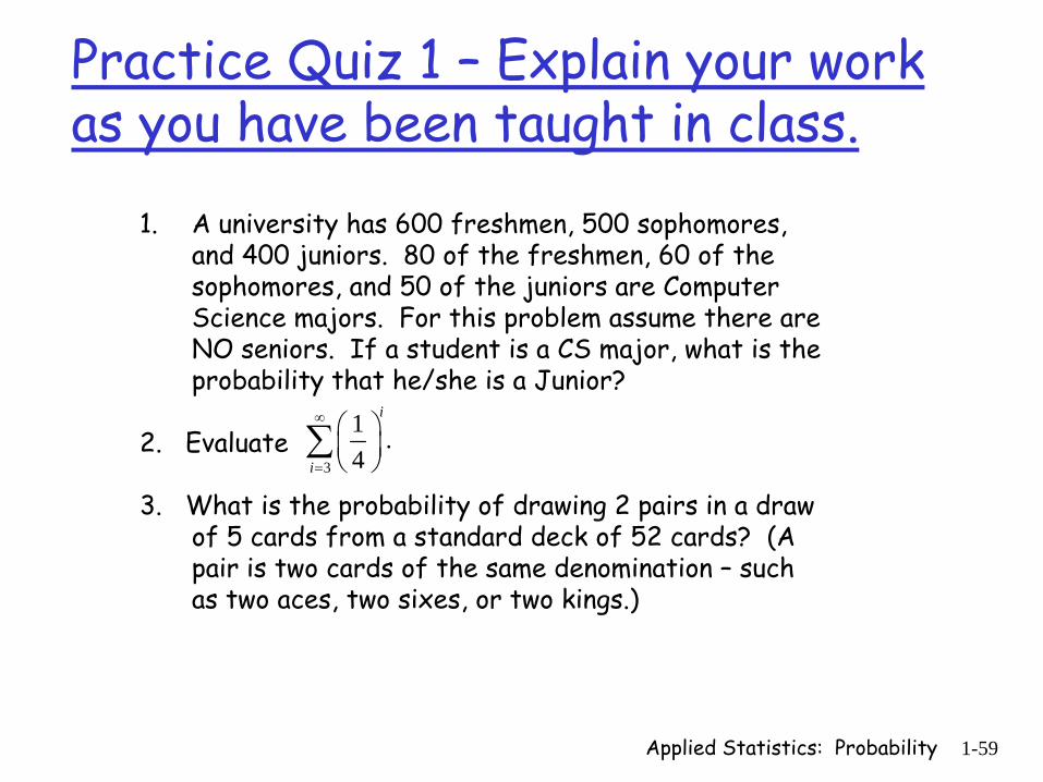
Practice Quiz 1 – Explain your work as you have been taught in class.
1. A university has 600 freshmen, 500 sophomores, and 400 juniors. 80 of the freshmen, 60 of the sophomores, and 50 of the juniors are Computer Science majors. For this problem assume there are NO seniors. If a student is a CS major, what is the probability that he/she is a Junior?
2. Evaluate
3. What is the probability of drawing 2 pairs in a draw of 5 cards from a standard deck of 52 cards? (A pair is two cards of the same denomination – such as two aces, two sixes, or two kings.)
3
1 .4
i
i
∞
=
⎛ ⎞⎜ ⎟⎝ ⎠
∑
Applied Statistics: Probability 1-60
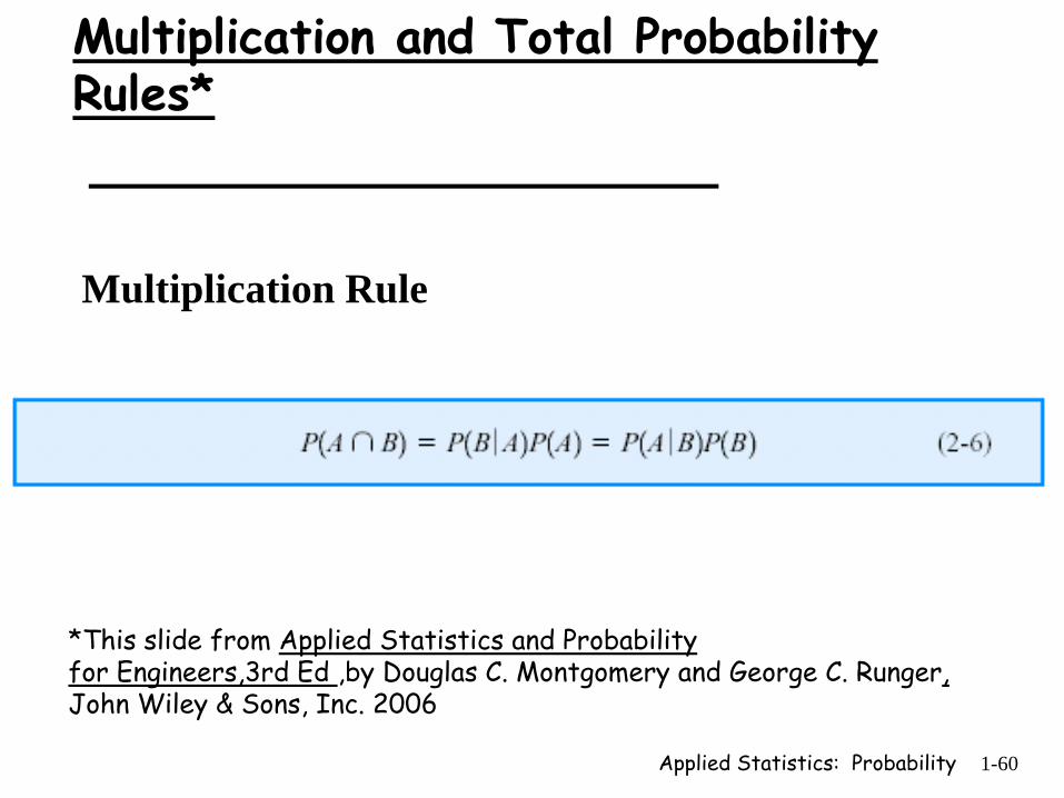
Multiplication and Total Probability Rules*
Multiplication Rule
*This slide from Applied Statistics and Probability for Engineers,3rd Ed ,by Douglas C. Montgomery and George C. Runger, John Wiley & Sons, Inc. 2006
Applied Statistics: Probability 1-61
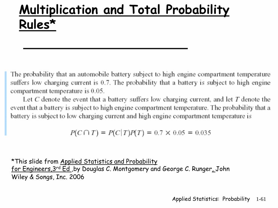
Multiplication and Total Probability Rules*
*This slide from Applied Statistics and Probability for Engineers,3rd Ed ,by Douglas C. Montgomery and George C. Runger, John Wiley & Songs, Inc. 2006
Applied Statistics: Probability 1-62
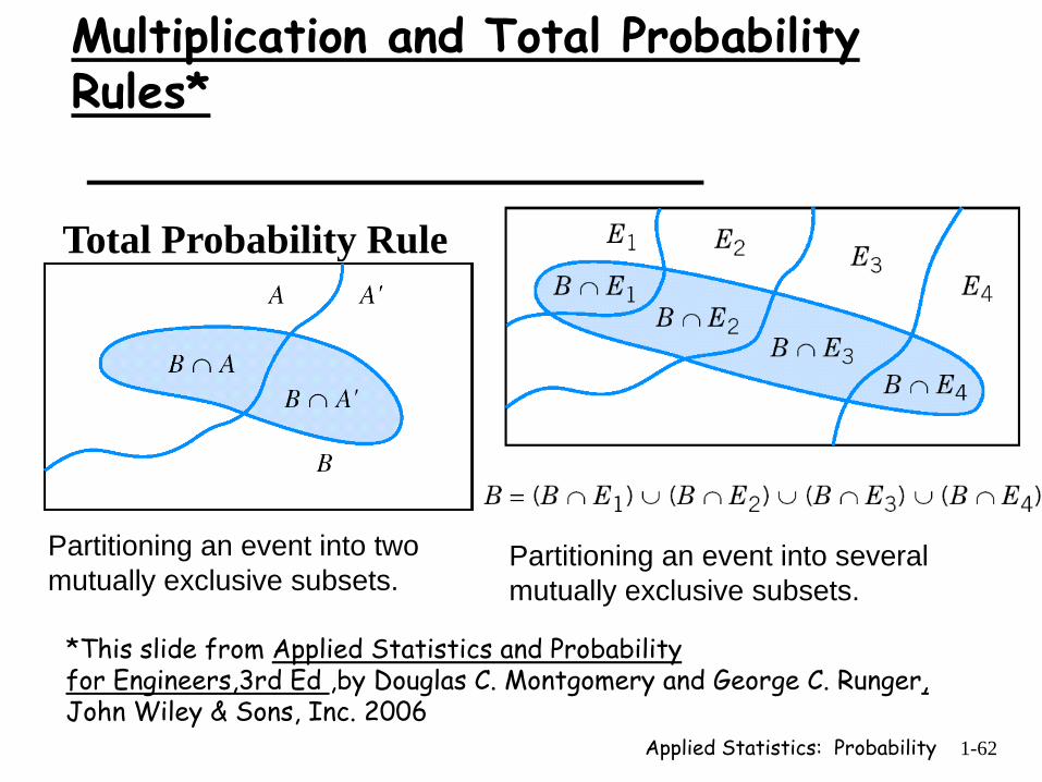
Multiplication and Total Probability Rules*
Total Probability Rule
Partitioning an event into two mutually exclusive subsets.
Partitioning an event into several mutually exclusive subsets.
*This slide from Applied Statistics and Probability for Engineers,3rd Ed ,by Douglas C. Montgomery and George C. Runger, John Wiley & Sons, Inc. 2006
Applied Statistics: Probability 1-63
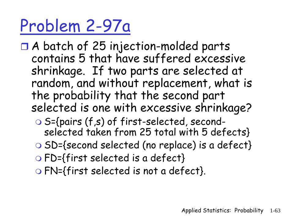
Problem 2-97aA batch of 25 injection-molded parts contains 5 that have suffered excessive shrinkage. If two parts are selected at random, and without replacement, what is the probability that the second part selected is one with excessive shrinkage?
S={pairs (f,s) of first-selected, second-selected taken from 25 total with 5 defects}SD={second selected (no replace) is a defect}FD={first selected is a defect}FN={first selected is not a defect}.

Applied Statistics: Probability 1-64
Problem Solution
We seek P[SD]=P[SD FD]+P[SD FN]This becomes
∩ ∩[ | ] [ ] [ | ] [ ]P SD FN P FN P SD FD P FD+
5 4 4 5 1 1 1* * 0.2.24 5 24 25 6 30 5
= + = + = =
Applied Statistics: Probability 1-65
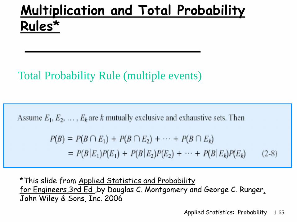
Multiplication and Total Probability Rules*
Total Probability Rule (multiple events)
*This slide from Applied Statistics and Probability for Engineers,3rd Ed ,by Douglas C. Montgomery and George C. Runger, John Wiley & Sons, Inc. 2006
Applied Statistics: Probability 1-66
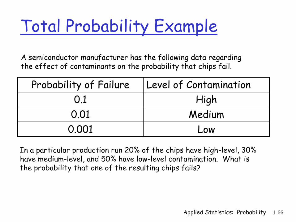
Total Probability ExampleA semiconductor manufacturer has the following data regarding the effect of contaminants on the probability that chips fail.
Probability of Failure Level of Contamination0.1 High
0.01 Medium0.001 Low
In a particular production run 20% of the chips have high-level, 30% have medium-level, and 50% have low-level contamination. What is the probability that one of the resulting chips fails?
Applied Statistics: Probability 1-67
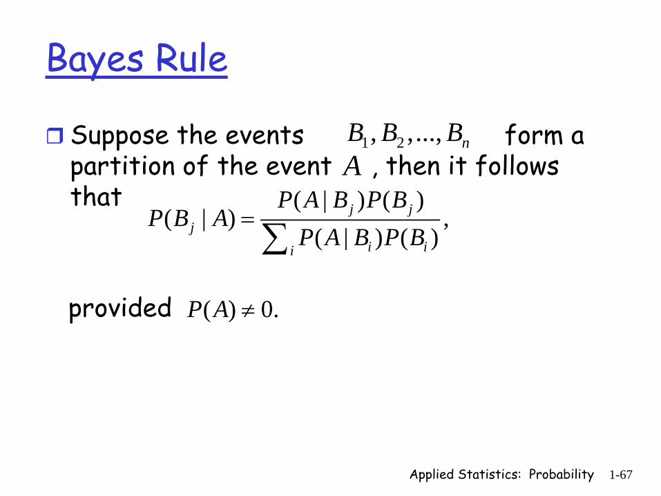
Bayes Rule
Suppose the events form a partition of the event , then it follows that
provided
A( | ) ( )
( | ) ,( | ) ( )
j jj
i ii
P A B P BP B A
P A B P B=
∑
( ) 0.P A ≠
1 2, ,..., nB B B
Applied Statistics: Probability 1-68
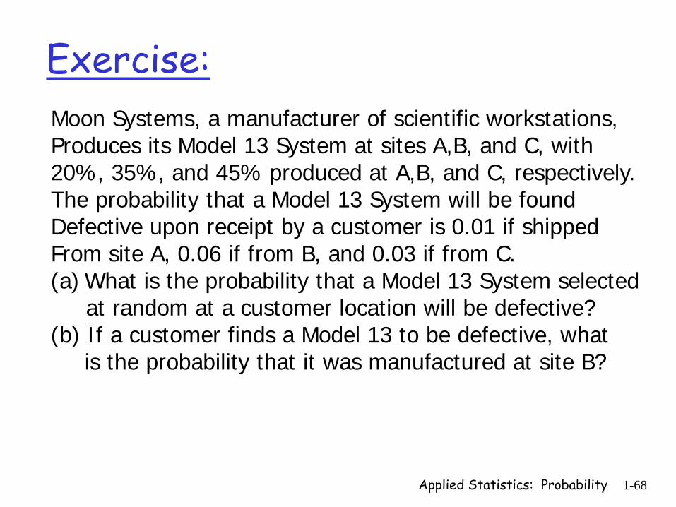
Exercise:Moon Systems, a manufacturer of scientific workstations,Produces its Model 13 System at sites A,B, and C, with 20%, 35%, and 45% produced at A,B, and C, respectively.The probability that a Model 13 System will be found Defective upon receipt by a customer is 0.01 if shipped From site A, 0.06 if from B, and 0.03 if from C.(a) What is the probability that a Model 13 System selected
at random at a customer location will be defective?(b) If a customer finds a Model 13 to be defective, what
is the probability that it was manufactured at site B?
Applied Statistics: Probability 1-69
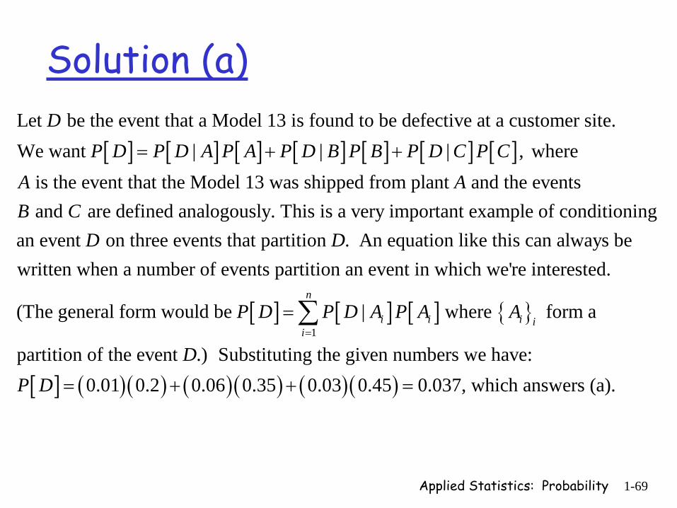
Solution (a)
[ ] [ ] [ ] [ ] [ ] [ ] [ ]Let be the event that a Model 13 is found to be defective at a customer site.We want | | | , where
is the event that the Model 13 was shipped from plant and the events and a
DP D P D A P A P D B P B P D C P C
A AB C
= + +
re defined analogously. This is a very important example of conditioningan event on three events that partition . An equation like this can always be written when a number of events partition an e
D D
[ ] [ ] [ ] { }
[ ] ( )( ) ( )( ) ( )( )
1
vent in which we're interested.
(The general form would be | where form a
partition of the event .) Substituting the given numbers we have:0.01 0.2 0.06 0.35 0.03 0.45 0.037, whic
n
i i i ii
P D P D A P A A
DP D
=
=
= + + =
∑
h answers (a).

Applied Statistics: Probability 1-70
Solution (b)
( | ) ( )Now we seek ( | )( | ) ( ) ( | ) ( ) ( | ) ( )
by Bayes Law. Substituting we get(0.06) (0.35) ( | )
(0.01) (0.2) (0.06) (0.35) (0.03) (0.45)
P D B P BP B DP D A P A P D B P B P D C P C
P B D
=+ +
×=
× + × + × 0.575=
(b) If a customer finds a Model 13 to be defective, what is the probability that it was manufactured at site B?
Applied Statistics: Probability 1-71
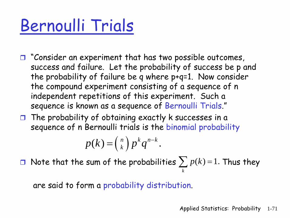
Bernoulli Trials
“Consider an experiment that has two possible outcomes, success and failure. Let the probability of success be p and the probability of failure be q where p+q=1. Now consider the compound experiment consisting of a sequence of n independent repetitions of this experiment. Such a sequence is known as a sequence of Bernoulli Trials.”The probability of obtaining exactly k successes in a sequence of n Bernoulli trials is the binomial probability
Note that the sum of the probabilities Thus they
are said to form a probability distribution.
( )( ) .n k n kkp k p q −=
( ) 1.k
p k =∑
Applied Statistics: Probability 1-72
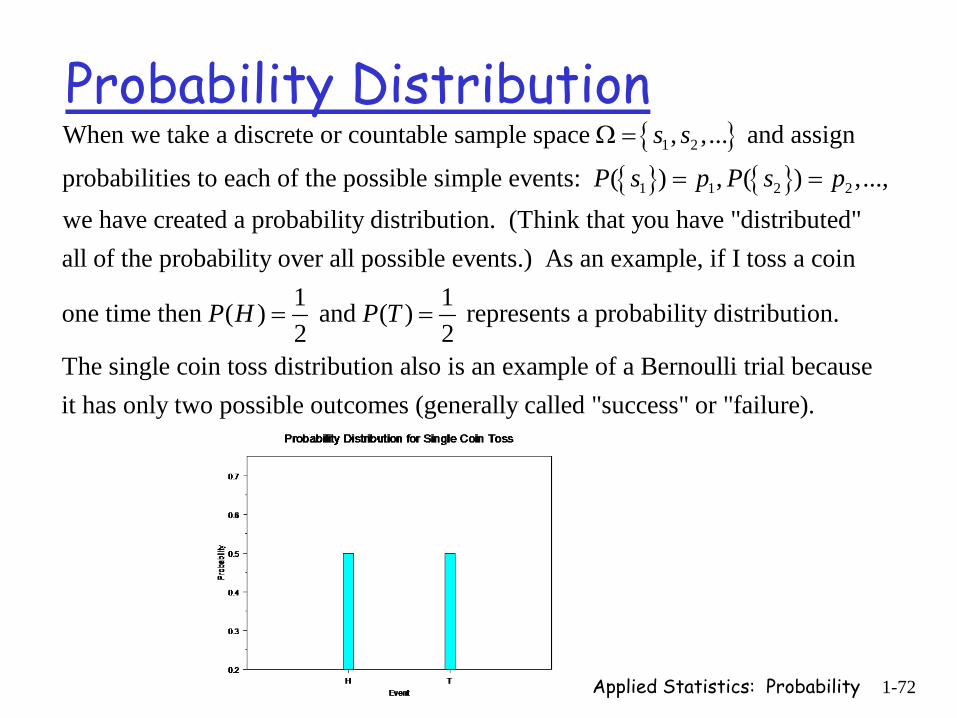
Probability Distribution{ }
{ } { }1 2
1 1 2 2
When we take a discrete or countable sample space , ,... and assign
probabilities to each of the possible simple events: ( ) , ( ) ,...,we have created a probability distribution. (Think
s s
P s p P s p
Ω =
= =
that you have "distributed"all of the probability over all possible events.) As an example, if I toss a coin
1 1one time then ( ) and ( ) represents a probability distribution. 2 2
The single coin
P H P T= =
toss distribution also is an example of a Bernoulli trial becauseit has only two possible outcomes (generally called "success" or "failure).

Applied Statistics: Probability 1-73
Binomial Probability Distribution( )The binomial probabilities are defined by ( ) , where
is the probability of success and is the probability of failure in Bernoullitrials. Suppose we toss a coin 10 times and we want the
n k n kkp k p q
p q n
−=
[ ] [ ]total number of heads.
Then , q , 10. Using the above formula we obtain the probabilities:
p P H P T n= = =
Binomial n=10 p=0.5
0.00E+00
5.00E-02
1.00E-01
1.50E-01
2.00E-01
2.50E-01
3.00E-01
0 1 2 3 4 5 6 7 8 9 10
probabilities

Applied Statistics: Probability 1-74
Regarding Parameters
( )Notice that the binomial distribution is completely defined by the formula
for its probabilities, ( ) , and by it "parameters" and .
The binomial probability equation never changes so we r
n k n kkp k p q p n−=
egard a binomial distribution as being defined by its parameters. This is typical of all probabilitydistributions (using their own parameters, of course).
One of the problems we often face in statistics is estimating the parametersafter collecting data that we know (or believe) comes from a particular probability distribution (such as the and for the binomial). Alternatively, we may choose
p nto estimate "statistics" such as mean and variance that are
functions of these parameters. We'll get to this, after we consider randomvariables and the the continuous sample space.
Applied Statistics: Probability 1-75
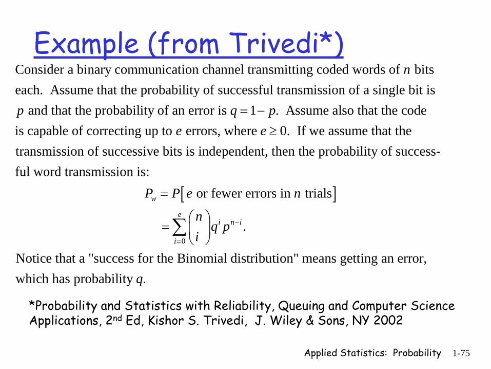
Example (from Trivedi*)Consider a binary communication channel transmitting coded words of bitseach. Assume that the probability of successful transmission of a single bit is
and that the probability of an error is 1
n
p q = . Assume also that the codeis capable of correcting up to errors, where 0. If we assume that the transmission of successive bits is independent, then the probability of success-ful word transm
pe e
−≥
[ ]
0
ission is: or fewer errors in trials
.
Notice that a "success for the Binomial distribution" me
w
ei n i
i
P P e n
nq p
i−
=
=
⎛ ⎞= ⎜ ⎟
⎝ ⎠∑
ans getting an error,which has probability .q
*Probability and Statistics with Reliability, Queuing and Computer Science Applications, 2nd Ed, Kishor S. Trivedi, J. Wiley & Sons, NY 2002
Applied Statistics: Probability 1-76
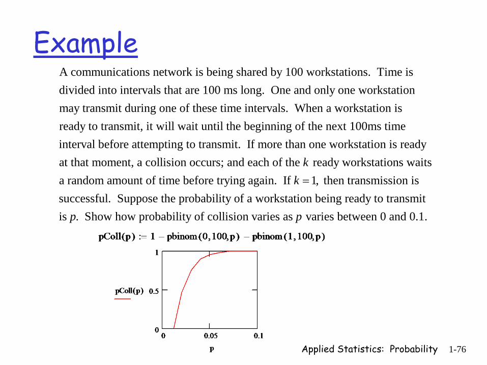
ExampleA communications network is being shared by 100 workstations. Time is divided into intervals that are 100 ms long. One and only one workstationmay transmit during one of these time intervals. When a workstation is ready to transmit, it will wait until the beginning of the next 100ms time interval before attempting to transmit. If more than one workstation is readyat that moment, a collision occurs; and each of the ready workstations waitsa random amount of time before trying again. If 1, then transmission is successful. Suppose the probability of a workstation being ready to transmit
kk =
is . Show how probability of collision varies as varies between 0 and 0.1. p p

Applied Statistics: Probability 1-77
Practice Quiz 2A partial deck of playing cards (fewer than 52 cards) contains some spades, hearts, diamonds, and clubs (NOT 13 of each “suit”). If a card is drawn at random, then the probability that it is a spade is 0.2. We write this as P[Spade]=0.2. Similarly, P[Heart]=0.3, P[Diamond]=0.25, P[Club]=0.25. Each of the 4 suits has some number of “face” cards (King, Queen, Jack). If the drawn card is a spade, the probability is 0.25 that it is a face card. If it is a heart, the probability is 0.25 that it is a face card. If it is a diamond, the probability is 0.2 that it is a face card. If it is a club, the probability is 0.1, that it is a face card.
1. What is the probability that the randomly drawn card is a face card?
2. What is the probability that the card is a Heart and a face card?
3. If the card is a face card, what is the probability that it is a spade?
Applied Statistics: Probability 1-78
Discrete Random Variables
G. A. Marin
Applied Statistics: Probability 1-79
Review of “function”
( ) ( ) ( ){ }
Defn: A function is a set of ordered pairs such that no two pairs have the samefirst element (unless they also have the same second element).
Example: 1,2 , 3, 5 , 5,12 defines a function, , whose "dg g=
2
omain"
consists of the real numbers 1,3,5 and whose "range" consists of the numbers
2, 5,12. All functions are said to "map" values in their domain to values intheir range. Example: ( ) 5. Heref x x= +
( ){ }2
a function is defined using a formula.
This actually implies the the function is , 5 : is a real number .
Notice the following:(a) The function has a "name." Here that name is .(b) The implied
f x x x
f
= +
domain of the function includes all real numbers, , that can be plugged into the formula. In this case that includes all real no's.(c) Every number in the domain (all reals) is "mapped" to
x
x
{ }
2 2
2
the number +5. Thus (1) 6, ( 5) 30, ( ) +5.(d) Sometimes we write this as 1 6, -5 30, +5. (e) The range of is : 5 .
x f f f
f x x
π π
π π
= − = =
→ → →
≥
Applied Statistics: Probability 1-80
Random Variable
Definition: A random variable on a sample space is a function that assigns a real number to each sample point The inverse image of is the set of all points in that the random variable maps to the value .It is denoted
X
( )X s
.s ∈Ω
x
Ω
X
x
{ | ( ) }.xA s X s x= ∈Ω =
Ω
discrete discreteXΩ ⇒
continuous continuousXΩ ⇒
Applied Statistics: Probability 1-81
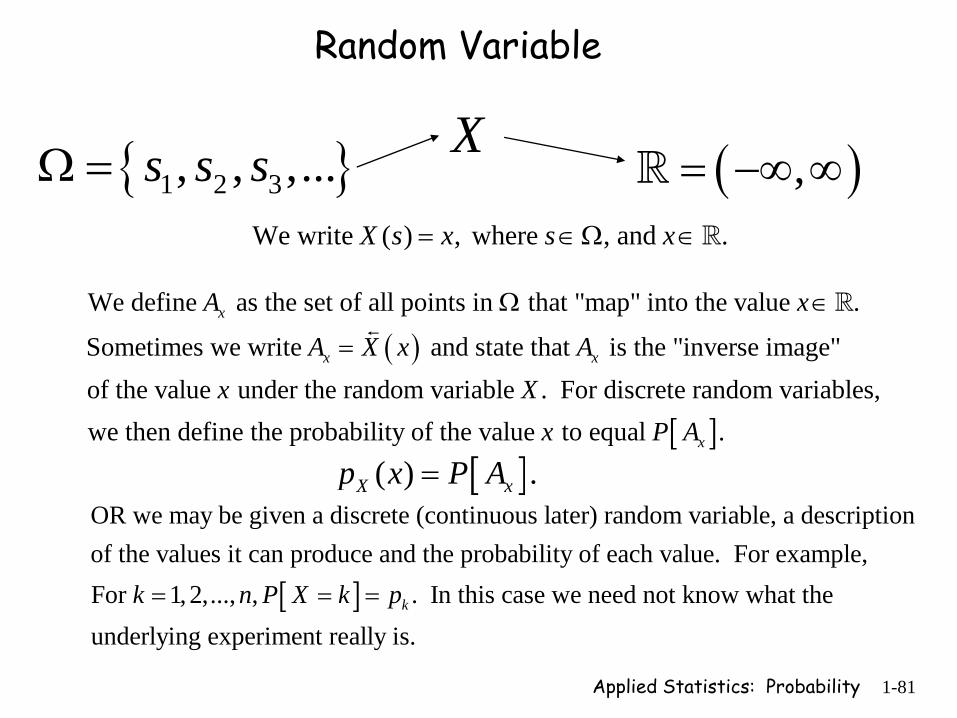
{ }1 2 3, , ,...s s sΩ = ( ),= −∞ ∞
( )We define as the set of all points in that "map" into the value .
Sometimes we write and state that is the "inverse image" of the value under the random variable . For discrete ra
x
x x
A x
A X x Ax X
Ω ∈
=
[ ]ndom variables,
we then define the probability of the value to equal .xx P A
X
Random Variable
[ ]( ) .X xp x P A=
We write ( ) , where , and .X s x s x= ∈Ω ∈
[ ]
OR we may be given a discrete (continuous later) random variable, a descriptionof the values it can produce and the probability of each value. For example,For 1,2,..., , . In this case we nekk n P X k p= = = ed not know what the underlying experiment really is.

Applied Statistics: Probability 1-82
The role of a random variableExperiment 1: Roll 1 fair die and determine the outcome. Experiment 2: Spin an arrow that lands with equal probability on one of the numbers 1 through 6.Experiment 3: You have 6 cards numbered 1 through 6. Shuffle them and draw one at random. Replace the card and reshuffle to repeat.
Notice that we’d represent the sample space of each of these as {1,2,3,4,5,6} usually without drawing dice or arrows or cards, but the sample spaces really include dice, arrows, cards.
For each probability distribution1let for 1, 2,...6.6ip i= =
The importance of the random variable is that it lets us deal with such an experimental setup without thinking dice, arrows, or cards.We say: “Let X be a random variable such that takes on the discrete values 1,2,3,4,5,6. Its probability mass function is given as:
the probability that X=i is 1/6. We write this as
1( ) for i=1,2,...,6.6Xp i =
Applied Statistics: Probability 1-83
Probability Mass FunctionIf is a discrete random variable, then its probability mass function (pmf) is given by: ( ) ( ) ( ) ( ).
x
X xs A
X
p x P X x P A P s∈
= = = = ∑
{ }1 2
The pmf satisfies the following properties:(p1) 0 ( ) 1 for all values, , such that [ ] is defined.(p2) If X is a discrete random var iable then ( ) 1, where the set , , ... includes
X
X ii
p x x P X x
p x x x
≤ ≤ =
=∑ all real
numbers, , such that ( ) 0.Xx p x ≠
Note: you cannot define a pmf without first defining a random variable. You can, however, define a probability distribution directly on a sample space with no random variable defined.
Applied Statistics: Probability 1-84
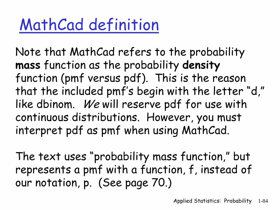
MathCad definitionNote that MathCad refers to the probability mass function as the probability densityfunction (pmf versus pdf). This is the reason that the included pmf’s begin with the letter “d,” like dbinom. We will reserve pdf for use with continuous distributions. However, you must interpret pdf as pmf when using MathCad.
The text uses “probability mass function,” but represents a pmf with a function, f, instead of our notation, p. (See page 70.)
Applied Statistics: Probability 1-85
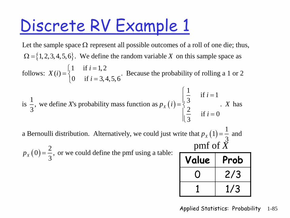
Discrete RV Example 1{ }
Let the sample space represent all possible outcomes of a roll of one die; thus, 1, 2,3,4,5,6 . We define the random variable on this sample space as
1 if 1,2follows: ( )
0 if 3, 4,
X
iX i
i
Ω
Ω =
==
=
( )
. Because the probability of rolling a 1 or 25,6
1 if 11 3is , we define 's probability mass function as . has
23 if 03
a Bernoulli distribution. Alternatively, we could j
X
iX p i X
i
⎧⎨⎩
⎧ =⎪⎪= ⎨⎪ =⎪⎩
( )
( )
1ust write that 1 and 3
20 , or we could define the pmf using a table:3
X
X
p
p
=
=Value Prob
0 2/31 1/3
pmf of X

Applied Statistics: Probability 1-86
Discrete RV Example 2A die is tossed until the occurrence of the first 6. Let the random variable
if the first 6 occurs on the roll for integer 0. What is theprobability mass function (pmf) for ?
In order fo
X k kth kX
= >
r the first 6 to occur on the 5th toss, for example, we must havethe event AAAA6 occur where A means any result other than 6. Clearly, these represent a sequence of 5 Bernoulli trials where success =
4
6 and failure = 1 through 5. Each trial is independent; thus, the probability
5 1 625of this particular result is 0.08. Similarly, the probability 6 6 7776
of the first 6 on the roll kth
⎛ ⎞ ⎛ ⎞ = =⎜ ⎟ ⎜ ⎟⎝ ⎠ ⎝ ⎠
1
1
5 1is . This defines the pmf, 6 6
5 1( ) . This is a particular instance of the geometric distribution.6 6
k
k
Xp k
−
−
⎛ ⎞ ⎛ ⎞⎜ ⎟ ⎜ ⎟⎝ ⎠ ⎝ ⎠
⎛ ⎞ ⎛ ⎞= ⎜ ⎟ ⎜ ⎟⎝ ⎠ ⎝ ⎠
Applied Statistics: Probability 1-87
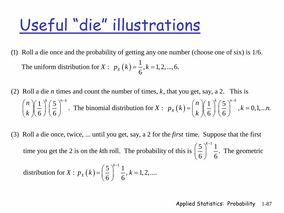
Useful “die” illustrations
( )
(1) Roll a die once and the probability of getting any one number (choose one of six) is 1/6.1 The uniform distribution for : , 1, 2,...,6.6
(2) Roll a die times and count the number of
XX p k k
n
= =
( )
times, , that you get, say, a 2. This is
1 5 1 5 . The binomial distribution for : , 0,1,... .6 6 6 6
(3) Roll a die once, twice, ... until yo
k n k k n k
X
k
n nX p k k n
k k
− −⎛ ⎞ ⎛ ⎞⎛ ⎞ ⎛ ⎞ ⎛ ⎞ ⎛ ⎞= =⎜ ⎟ ⎜ ⎟⎜ ⎟ ⎜ ⎟ ⎜ ⎟ ⎜ ⎟⎝ ⎠ ⎝ ⎠ ⎝ ⎠ ⎝ ⎠⎝ ⎠ ⎝ ⎠
( )
1
u get, say, a 2 for the time. Suppose that the first
5 1 time you get the 2 is on the th roll. The probability of this is . The geometric6 6
5 distribution for : 6
k
X
first
k
X p k
−⎛ ⎞⎜ ⎟⎝ ⎠
⎛ ⎞= ⎜⎝ ⎠
1 1 , 1, 2,....6
k
k−
=⎟
Applied Statistics: Probability 1-88
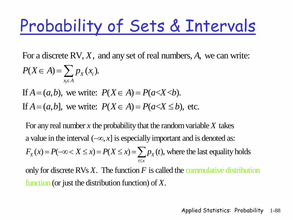
Probability of Sets & IntervalsFor a discrete RV, , and any set of real numbers, , we can write:
( ) ( ).
If ( , ), we write: ( ) ( < < ). If ( , ], we write: ( ) ( < ), etc.
i
X ix A
X AP X A p x
A a b P X A P a X bA a b P X A P a X b
∈
∈ =
= ∈ == ∈ = ≤
∑
For any real number the probability that the random variable takes a value in the interval ( , ] is especially important and is denoted as:
( ) ( ) ( ) ( ), where the last equalitX Xt x
x Xx
F x P X x P X x p t≤
−∞
= −∞< ≤ = ≤ =∑cummulative d
y holds
only f istributionfu
or discrete RVs . The function is called the (or just the distribution functionnction ) of .
X FX
Applied Statistics: Probability 1-89
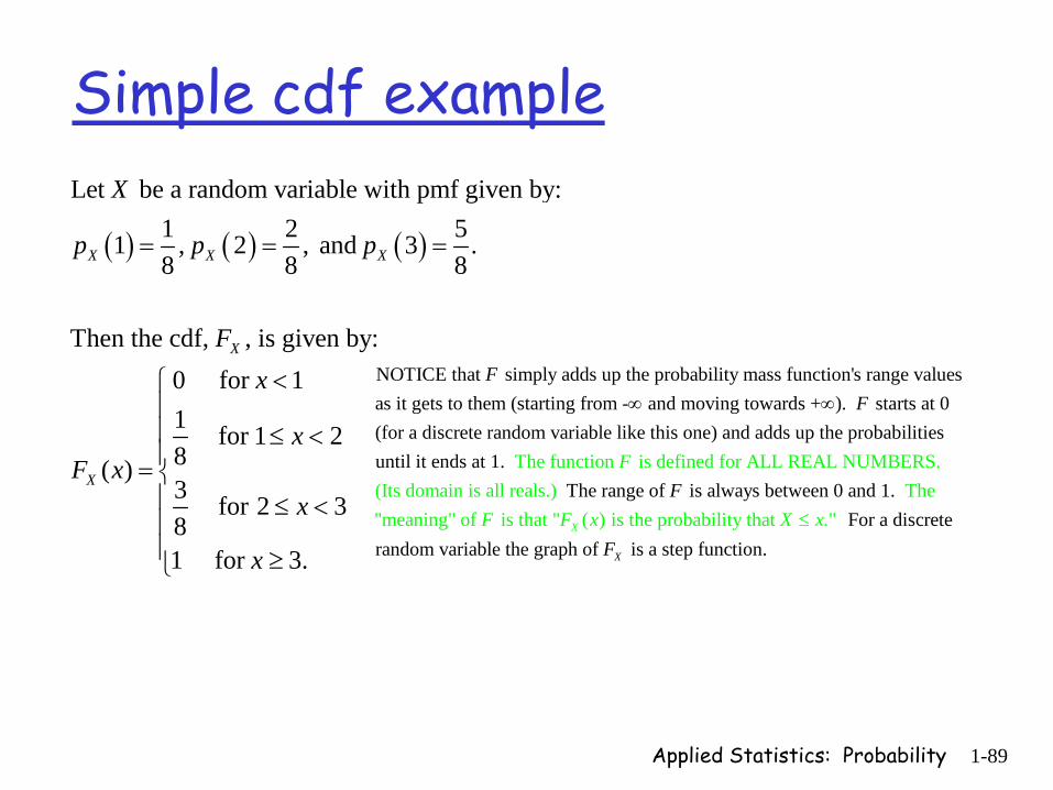
Simple cdf example
( ) ( ) ( )
Let be a random variable with pmf given by:1 2 51 , 2 , and 3 .8 8 8
Then the cdf, , is given by:0 for 11 for 1 28( )3 for 2 381 for 3.
X X X
X
X
X
p p p
Fx
xF x
x
x
= = =
<⎧⎪⎪ ≤ <⎪= ⎨⎪ ≤ <⎪⎪ ≥⎩
NOTICE that simply adds up the probability mass function's range valuesas it gets to them (starting from - and moving towards + ). starts at 0 (for a discrete random variable like this one) and
FF∞ ∞
The function is defined for ALL REAL NUMBERS.(Its do
adds up the probabilities until it ends at 1.
The range of is always betweenmain is all reals.) The "meaning" of is that " ( ) i
0 and 1.
X
F
F F xF
For a discrete random variable the gr
s the probabiaph of i
litys a
that ."step fun
ction.X
X xF
≤
Applied Statistics: Probability 1-90
Cumulative Distribution Function Properties
x - x
1 2
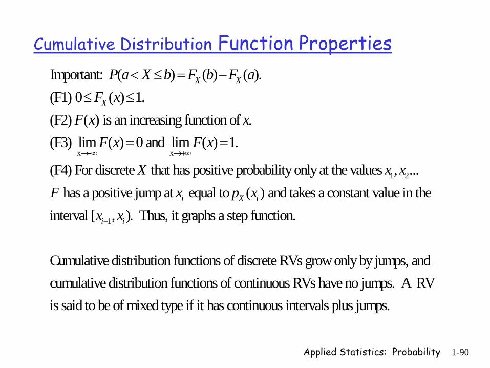
Important: ( ) ( ) ( ).(F1) 0 ( ) 1.(F2) ( ) is an increasing function of .(F3) lim ( ) 0 and lim ( ) 1.
(F4) For discrete that has positive probability only at the values ,
X X
X
P a X b F b F aF x
F x xF x F x
X x x→ ∞ →+∞
< ≤ = −≤ ≤
= =
1
... has a positive jump at equal to ( ) and takes a constant value in the
interval [ , ). Thus, it graphs a step function.
Cumulative distribution functions of discrete RVs grow only by jum
i X i
i i
F x p xx x−
ps, and cumulative distribution functions of continuous RVs have no jumps. A RV is said to be of mixed type if it has continuous intervals plus jumps.
Applied Statistics: Probability 1-91
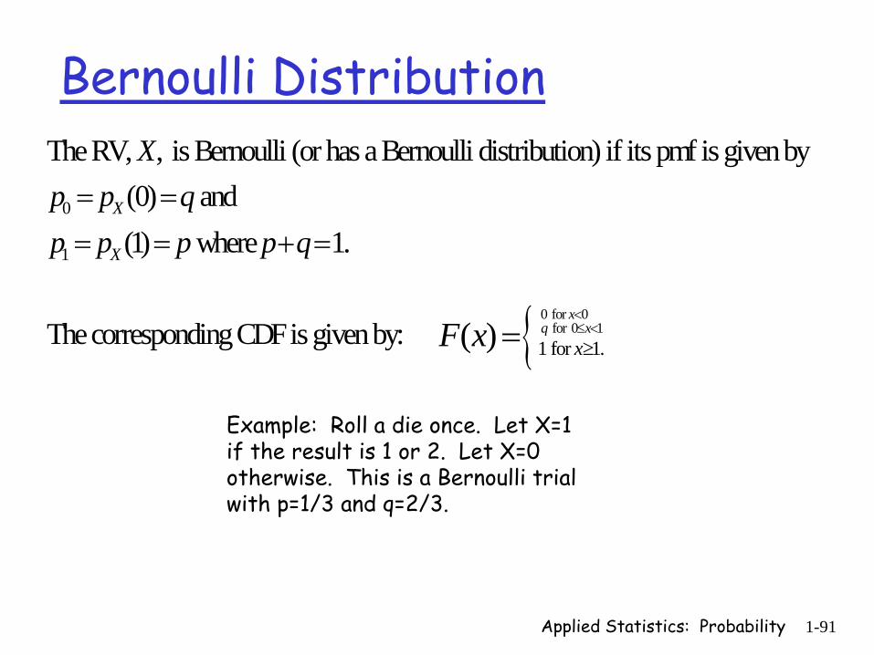
Bernoulli Distribution
0
1
The RV, , is Bernoulli (or has a Bernoulli distribution) if its pmf is given by(0) and (1) where 1.
The corresponding CDF is given by:
X
X
Xp p qp p p p q
= == = + =
{ 0 for 0 for 0 1
1 for 1.( )x
q xxF x<≤ <
≥=
Example: Roll a die once. Let X=1 if the result is 1 or 2. Let X=0 otherwise. This is a Bernoulli trial with p=1/3 and q=2/3.
Applied Statistics: Probability 1-92
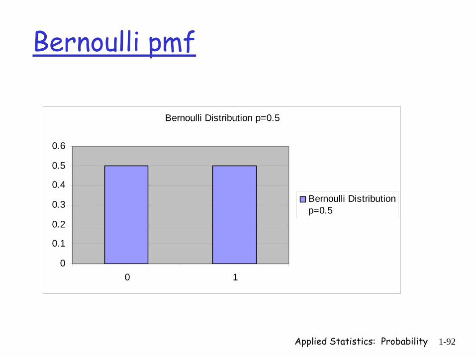
Bernoulli pmf
Bernoulli Distribution p=0.5
0
0.1
0.2
0.3
0.4
0.5
0.6
0 1
Bernoulli Distributionp=0.5

Applied Statistics: Probability 1-93
Bernoulli cdf p=0.5
( )0 for 0
Write as: 0.5 for 0 11 otherwise.
Notice that the cdf is defined for all real numbers, .
xF x x
x
<⎧⎪= ≤ <⎨⎪⎩
Applied Statistics: Probability 1-94
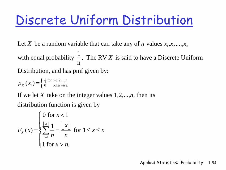
Discrete Uniform Distribution
1 2
0 otherwise.
Let be a random variable that can take any of values , ,...,1with equal probability . The RV is said to have a Discrete Uniformn
Distribution, and has pmf given by:
( )
n
X i
X n x x x
X
p x = { 1 for 1,2,...,
1
If we let take on the integer values 1,2,..., , then its distribution function is given by
0 for 1
1( ) for 1
1 for .
n i n
x
Xi
X n
xx
F x x nn n
x n
=
⎢ ⎥⎣ ⎦
=
<⎧⎪
⎢ ⎥⎪ ⎣ ⎦= = ≤ ≤⎨⎪⎪ >⎩
∑
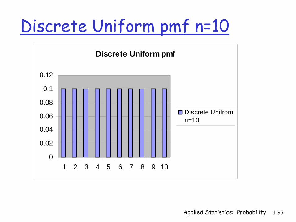
Applied Statistics: Probability 1-95
Discrete Uniform pmf n=10Discrete Uniform pmf
0
0.02
0.04
0.06
0.08
0.1
0.12
1 2 3 4 5 6 7 8 9 10
Discrete Unifromn=10
Applied Statistics: Probability 1-96
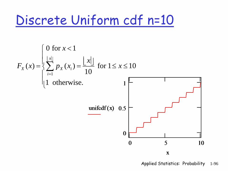
Discrete Uniform cdf n=10
1
0 for 1
( ) ( ) for 1 1010
1 otherwise.
x
X X ii
xx
F x p x x⎢ ⎥⎣ ⎦
=
<⎧⎪
⎢ ⎥⎪ ⎣ ⎦= = ≤ ≤⎨⎪⎪⎩
∑
Applied Statistics: Probability 1-97
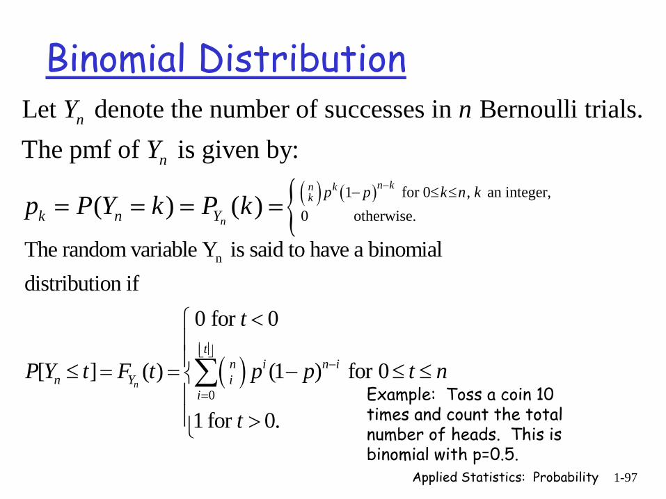
Binomial Distribution
( ) ( ){ 1 for 0 , an integer,0 otherwise.
Let denote the number of successes in Bernoulli trials.The pmf of is given by:
( ) ( )n kn k
k
n
n
n
p p k n kk n Y
Y nY
p P Y k P k−− ≤ ≤
= = = =
( )
n
0
The random variable Y is said to have a binomial distribution if
0 for 0
[ ] ( ) (1 ) for 0
1 for 0.
n
tn i n i
n Y ii
t
P Y t F t p p t n
t
⎢ ⎥⎣ ⎦−
=
<⎧⎪⎪≤ = = − ≤ ≤⎨⎪⎪ >⎩
∑Example: Toss a coin 10 times and count the total number of heads. This is binomial with p=0.5.
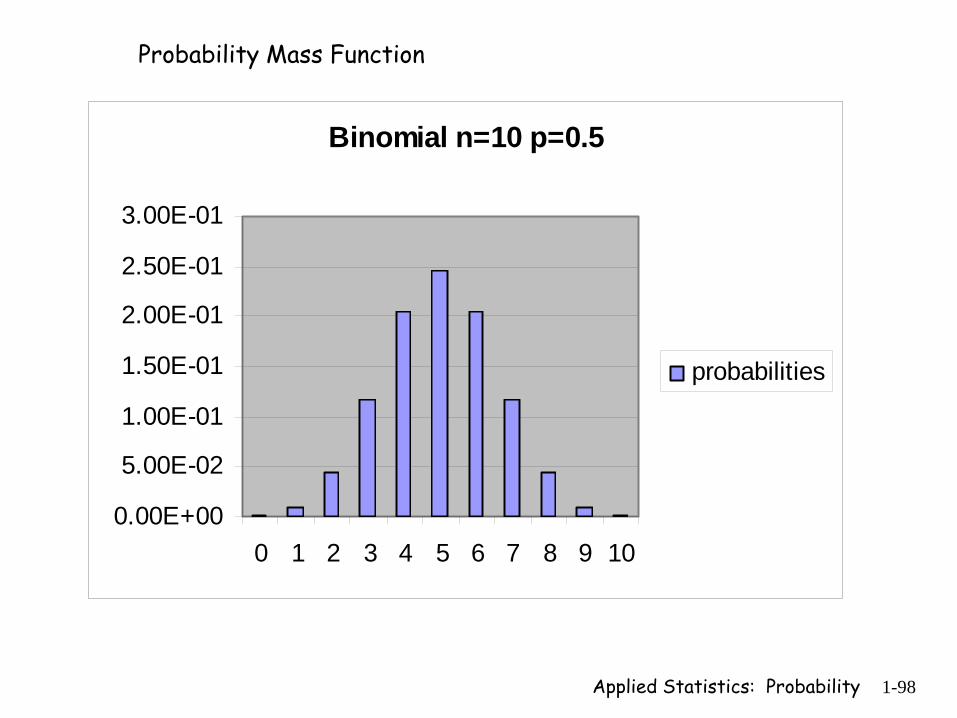
Applied Statistics: Probability 1-98
Binomial n=10 p=0.5
0.00E+00
5.00E-02
1.00E-01
1.50E-01
2.00E-01
2.50E-01
3.00E-01
0 1 2 3 4 5 6 7 8 9 10
probabilities
Probability Mass Function

Applied Statistics: Probability 1-99
Binomial cdf n=10 p=0.5
( )10 10
0
0 for 0
[ ] ( ) (1 ) for 0 10
1 otherwise.
n
ti i
n Y ii
t
P Y t F t p p t⎢ ⎥⎣ ⎦
−
=
<⎧⎪⎪≤ = = − ≤ ≤⎨⎪⎪⎩
∑
Applied Statistics: Probability 1-100
Geometric Distribution
1
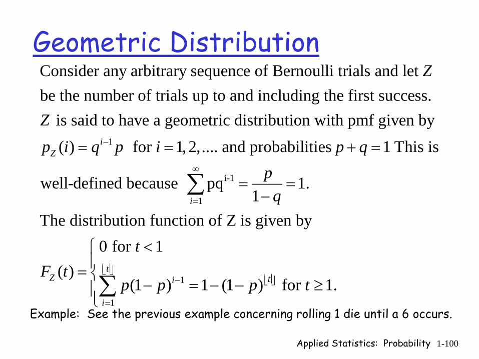
Consider any arbitrary sequence of Bernoulli trials and let be the number of trials up to and including the first success.
is said to have a geometric distribution with pmf given by( ) for i
Z
Z
Zp i q p−=
i-1
1
1
1
1, 2,.... and probabilities 1 This is
well-defined because pq 1. 1
The distribution function of Z is given by0 for 1
( )(1 ) 1 (1 ) for 1.
i
tZ ti
i
i p qpq
tF t
p p p t
∞
=
⎢ ⎥⎣ ⎦⎢ ⎥− ⎣ ⎦
=
= + =
= =−
<⎧⎪= ⎨
− = − − ≥⎪⎩
∑
∑Example: See the previous example concerning rolling 1 die until a 6 occurs.
Applied Statistics: Probability 1-101
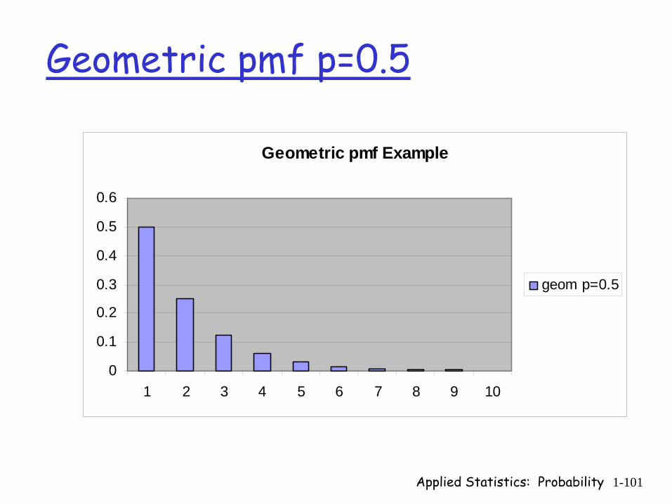
Geometric pmf Example
0
0.1
0.2
0.3
0.4
0.5
0.6
1 2 3 4 5 6 7 8 9 10
geom p=0.5
Geometric pmf p=0.5
Applied Statistics: Probability 1-102
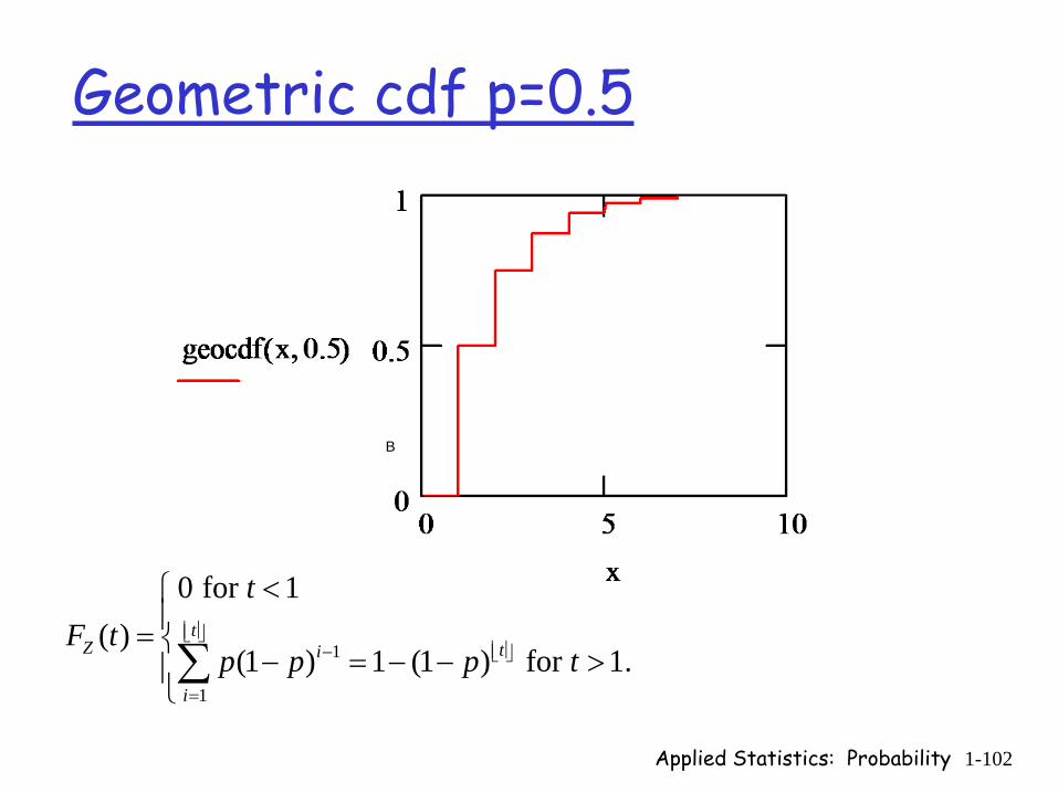
Geometric cdf p=0.5
1
1
0 for 1( )
(1 ) 1 (1 ) for 1.t
Z ti
i
tF t
p p p t⎢ ⎥⎣ ⎦
⎢ ⎥− ⎣ ⎦
=
<⎧⎪= ⎨
− = − − >⎪⎩∑
B
Applied Statistics: Probability 1-103
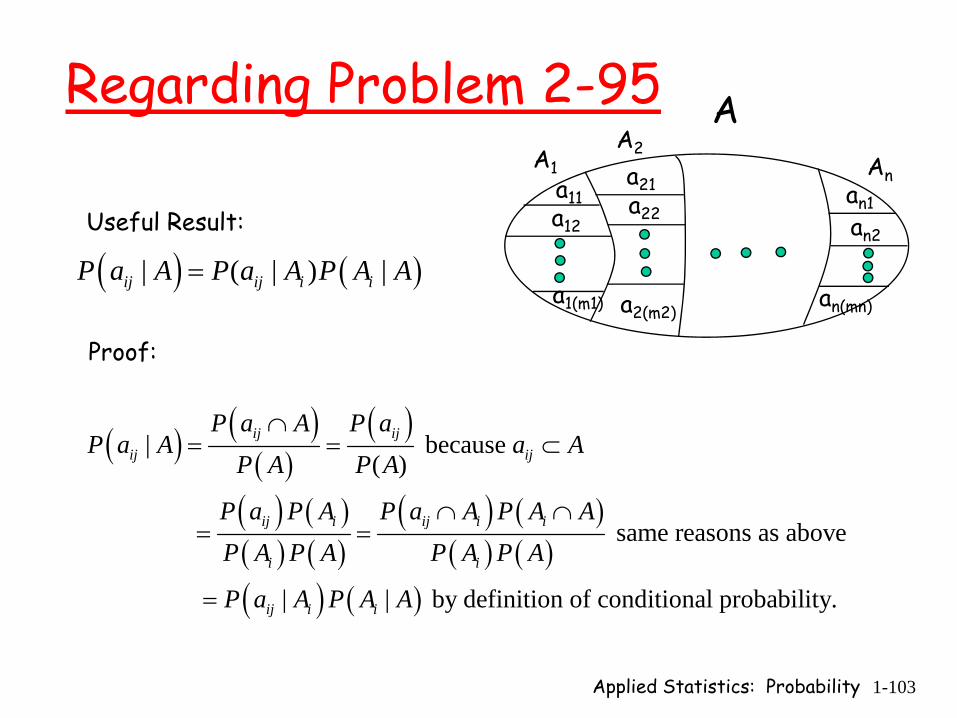
Regarding Problem 2-95A1
A2Ana11
a12
a1(m1)
a21a22
a2(m2)
an1an2
an(mn)
( ) ( )| ( | ) |ij ij i iP a A P a A P A A=
Useful Result:
Proof:
( ) ( )( )
( )
( ) ( )( ) ( )
( ) ( )( ) ( )
( ) ( )
| because ( )
same reasons as above
| | by definition of conditional probability.
ij ijij ij
ij i ij i i
i i
ij i i
P a A P aP a A a A
P A P A
P a P A P a A P A AP A P A P A P A
P a A P A A
∩= = ⊂
∩ ∩= =
=
A
Applied Statistics: Probability 1-104
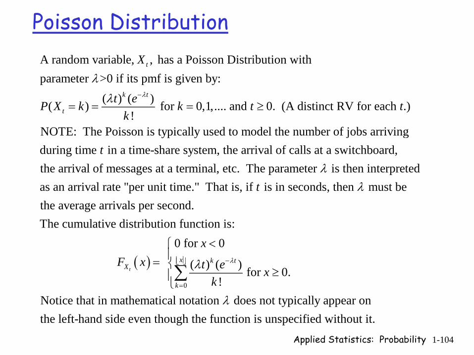
Poisson DistributionA random variable, , has a Poisson Distribution with parameter >0 if its pmf is given by:
( ) ( )( ) for 0,1,.... and 0. (A distinct RV for each .)!
NOTE: The Poisson is typically u
t
k t
t
X
t eP X k k t tk
λ
λ
λ −
= = = ≥
sed to model the number of jobs arrivingduring time in a time-share system, the arrival of calls at a switchboard, the arrival of messages at a terminal, etc. The parameter is then interpreted as
tλ
( )
an arrival rate "per unit time." That is, if is in seconds, then must bethe average arrivals per second. The cumulative distribution function is:
0 for 0 ( ) (t
kX
t
xF x t e
λ
λ −
<=
0
) for 0.!
Notice that in mathematical notation does not typically appear on the left-hand side even though the function is unspecified without it.
x t
k
xk
λ
λ
⎢ ⎥⎣ ⎦
=
⎧⎪⎨
≥⎪⎩∑
Applied Statistics: Probability 1-105
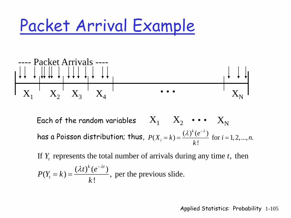
Packet Arrival Example
X1 X2 X3 X4 XN…
---- Packet Arrivals ----
Each of the random variables X1 X2 … XN
has a Poisson distribution; thus, ( ) ( )( ) for 1, 2,..., .!
k
ieP X k i n
k
λλ −
= = =
If represents the total number of arrivals during any time , then
( ) ( )( ) , per the previous slide. !
tk t
t
Y t
t eP Y kk
λλ −
= =
Applied Statistics: Probability 1-106
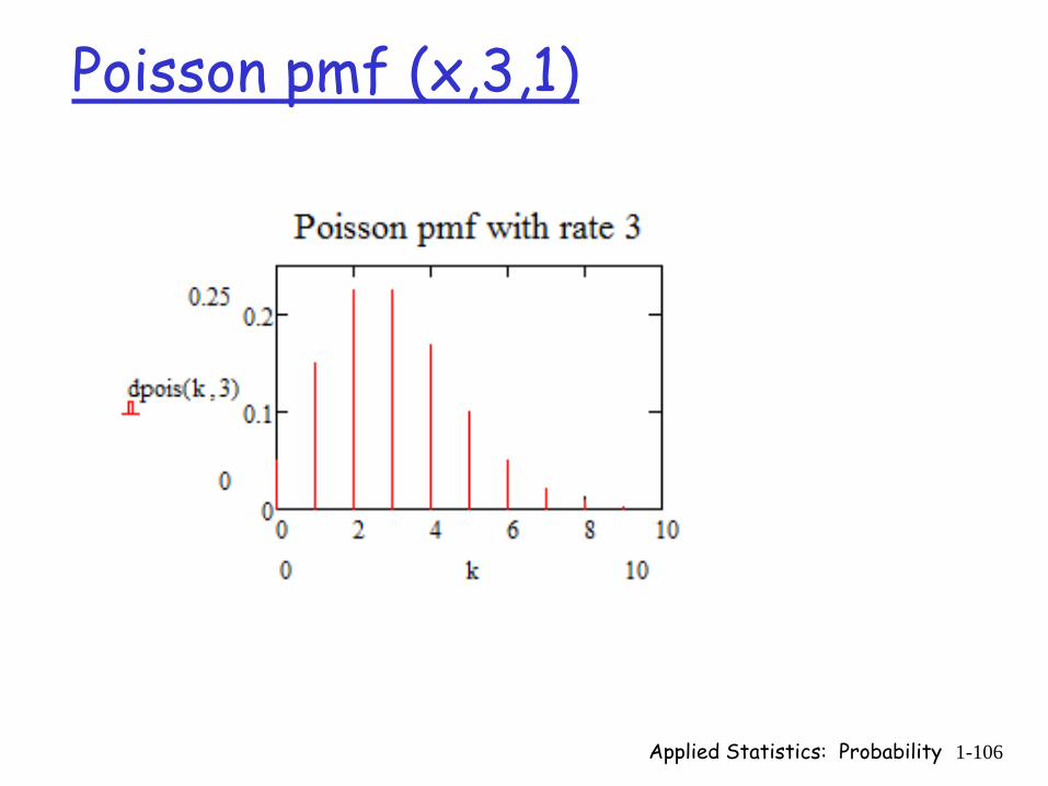
Poisson pmf (x,3,1)
Applied Statistics: Probability 1-107
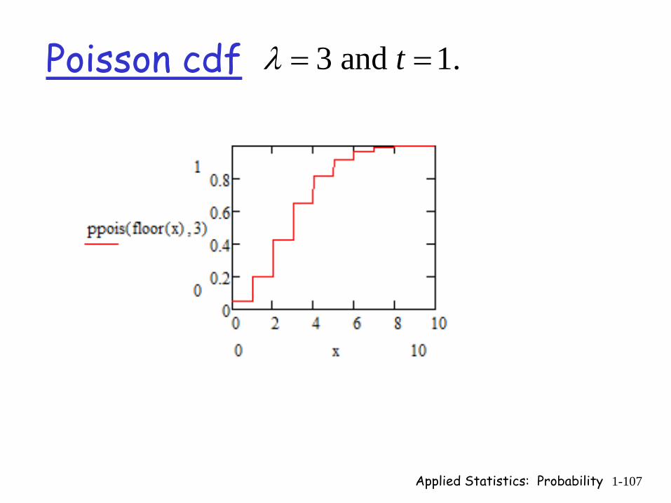
Poisson cdf 3 and 1.tλ = =

Applied Statistics: Probability 1-108
Poisson ExampleConnections arrive at a switch at a rate of 11 per ms. The arrival distribution is Poisson. (a) What is the probability that exactly 11 calls arrive in one ms? (b) What is the probabilitythat exactly 100 calls arrive in 10 ms? (c) What is the probability that the number of calls arriving in 2 ms is greater that 7 and less than or equal to 10?
[ ]( ) ( )
[ ]( ) ( )11
Let be the random variable giving the number of arrivals during ms. We know
that has a Poisson distribution, which implies that . The!
1111arrival rate is ; thus, ms
tk t
t t
k t
t
X t
t eX P X k
kt e
P X k
λλ −
−
= =
= =
[ ]( ) ( )
[ ]( ) ( )
[ ]( ) ( )
11 11
1
100 11 10
10
11 2
2
with in ms. !
11(a) Probability of exactly 11 arrivals in one ms is 11 0.119.
11!11 10
(b) Probability of 100 calls in 10 ms is 100 0.025.100!
11 2(c) 7 10
!
k
k
tk
eP X
eP X
eP X
k
−
− ×
− ×
=
= = =
×= = =
×< ≤ =
8 2 810
22 228
22 1 22 22 22 794 0.003.8! 9! 10! 10!e e
⎛ ⎞ ⎛ ⎞= + + = =⎜ ⎟ ⎜ ⎟⎝ ⎠⎝ ⎠
∑
Applied Statistics: Probability 1-109
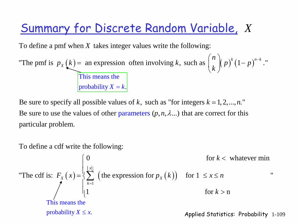
Summary for Discrete Random Variable, X
( ) ( ) ( )
To define a pmf when takes integer values write the following:
"The pmf is an expression often involving , such as 1 ."
Be sure to specify all possible values of , such as "for
k n kX
Xn
p k k p pk
k
−⎛ ⎞= −⎜ ⎟
⎝ ⎠
( )
integers 1, 2,..., ." Be sure to use the values of other ( , , ...) that are correct for thisparticular problem.
To define a cdf write the following:0
"T
par
he cdf is:
am e
et rs
X
k np n
F x
λ=
= ( )( )1
for whatever min
the expression for for 1 "
1 for n
x
Xk
k
p k x n
k
⎢ ⎥⎣ ⎦
=
<⎧⎪⎪ ≤ ≤⎨⎪⎪ >⎩
∑
This means theprobability .X k=
This means theprobability .X x≤
Applied Statistics: Probability 1-110
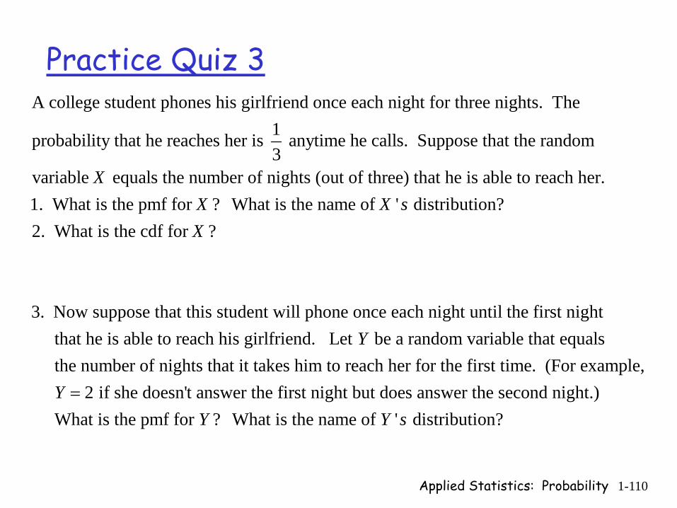
Practice Quiz 3A college student phones his girlfriend once each night for three nights. The
1probability that he reaches her is anytime he calls. Suppose that the random3
variable equals the number of nights (ouX t of three) that he is able to reach her. 1. What is the pmf for ? What is the name of ' distribution?2. What is the cdf for ?
3. Now suppose that this student will phone once each night until
X X sX
the first night that he is able to reach his girlfriend. Let be a random variable that equals the number of nights that it takes him to reach her for the first time. (For example,
Y
2 if she doesn't answer the first night but does answer the second night.) What is the pmf for ? What is the name of ' distribution?
YY Y s
=
Applied Statistics: Probability 1-111
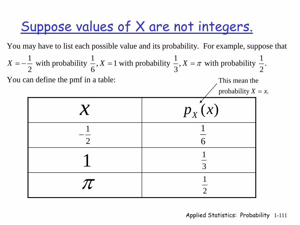
Suppose values of X are not integers.You may have to list each possible value and its probability. For example, suppose that
1 1 1 1 with probability , 1 with probability , with probability .2 6 3 2
You can define the pmf in a table:
X X X π= − = =
x ( )Xp x12
−16
1 13
π 12
This mean the probability .X x=
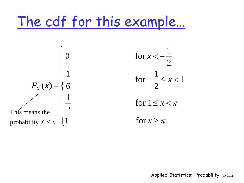
Applied Statistics: Probability 1-112
The cdf for this example…
10 for 2
1 1 for 1 ( ) 6 2
1 for 121 for .
X
x
xF x
x
x
π
π
⎧ < −⎪⎪⎪ − ≤ <⎪= ⎨⎪
≤ <⎪⎪⎪ ≥⎩
This means the probability .X x≤
Applied Statistics: Probability 1-113
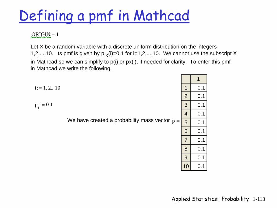
Defining a pmf in MathcadORIGIN 1:=
Let X be a random variable with a discrete uniform distribution on the integers1,2,...,10. Its pmf is given by p X(i)=0.1 for i=1,2,...,10. We cannot use the subscript Xin Mathcad so we can simplify to p(i) or px(i), if needed for clarity. To enter this pmfin Mathcad we write the following.
i 1 2, 10..:=
pi 0.1:=
We have created a probability mass vector p
1
12
3
4
5
6
7
8
9
10
0.10.1
0.1
0.1
0.1
0.1
0.1
0.1
0.1
0.1
=
Applied Statistics: Probability 1-114
Define pmf continued
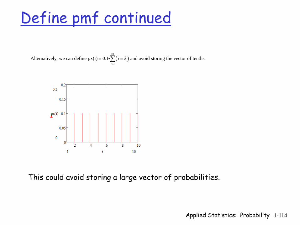
This could avoid storing a large vector of probabilities.
( )10
1Alternatively, we can define px(i) 0.1 and avoid storing the vector of tenths.
ii k
=
= =∑i

Applied Statistics: Probability 1-115
To define the corresponding cdfThe cdf can now be defined as:
FX x( ) 0 x 1<( )⋅
1
floor x( )
i
px i( )∑=
⎛⎜⎜⎝
⎞⎟⎟⎠
1 x≤ 10≤( )⋅+ 1 x 10>( )⋅+:=
0 5 100
0.2
0.4
0.6
0.8
1
FX x( )
x
Applied Statistics: Probability 1-116
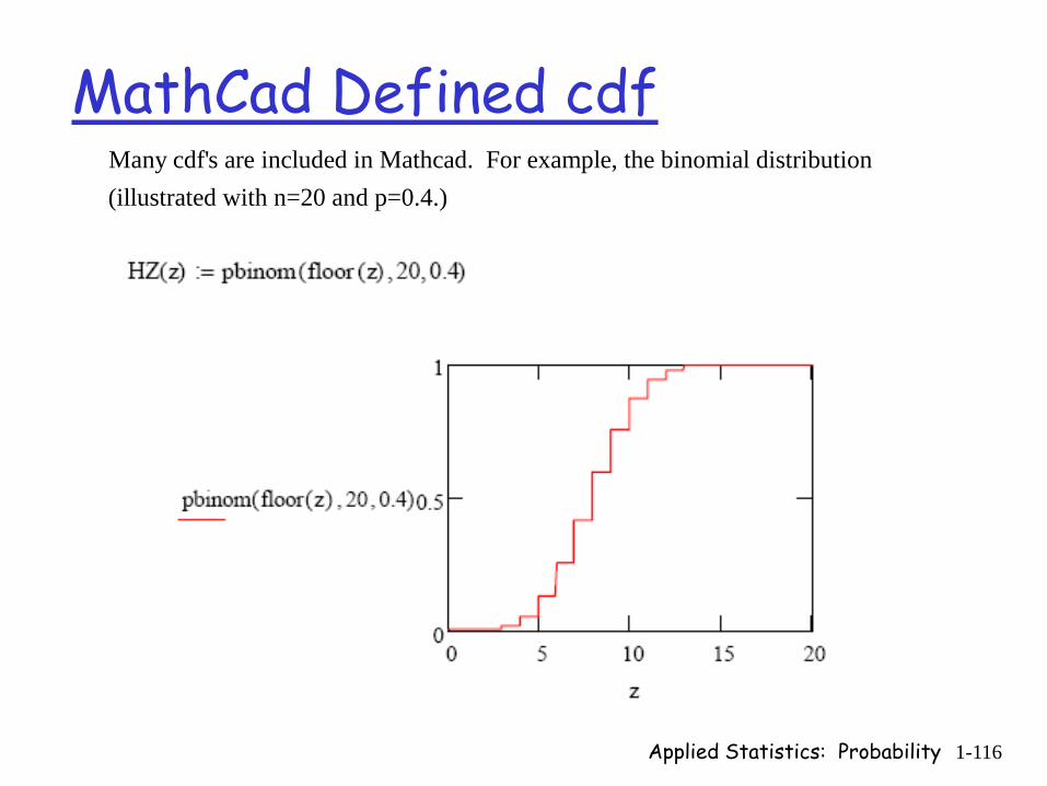
MathCad Defined cdfMany cdf's are included in Mathcad. For example, the binomial distribution (illustrated with n=20 and p=0.4.)

Applied Statistics: Probability 1-117
Mean and Variance of a Discrete Random VariableDefinition
2 2Working formula: ( ) ( ) ( ).Var X E X E X= −
Applied Statistics: Probability 1-118
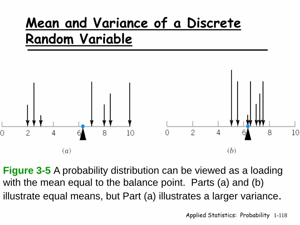
Mean and Variance of a Discrete Random Variable
Figure 3-5 A probability distribution can be viewed as a loading with the mean equal to the balance point. Parts (a) and (b) illustrate equal means, but Part (a) illustrates a larger variance.
Applied Statistics: Probability 1-119
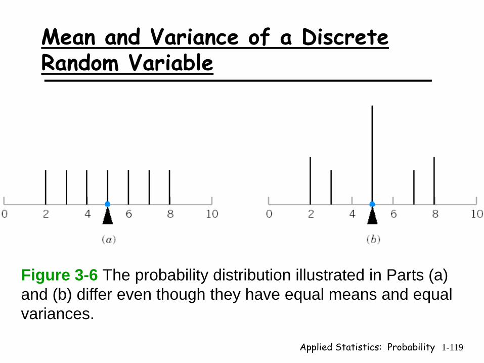
Mean and Variance of a Discrete Random Variable
Figure 3-6 The probability distribution illustrated in Parts (a) and (b) differ even though they have equal means and equal variances.
Applied Statistics: Probability 1-120
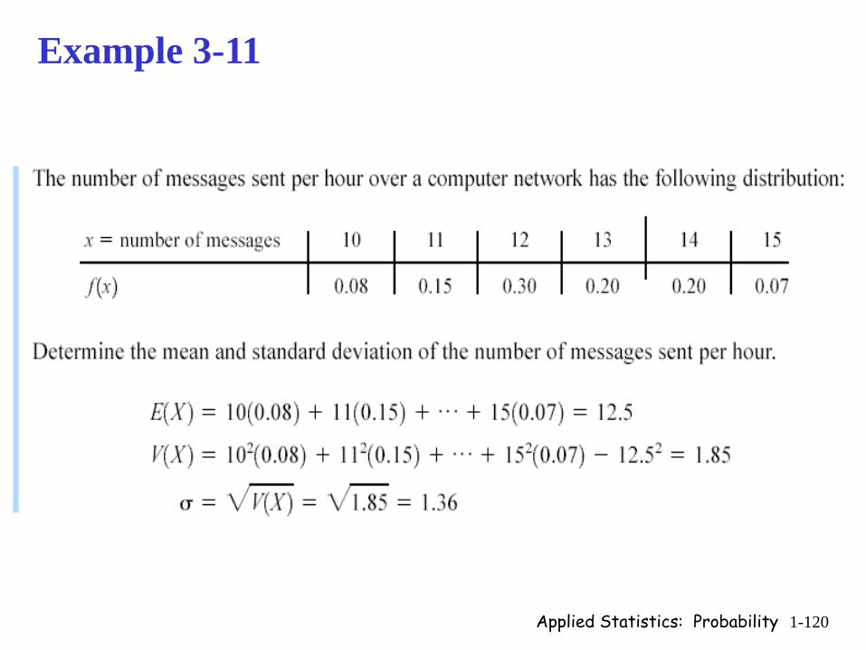
Example 3-11
Applied Statistics: Probability 1-121
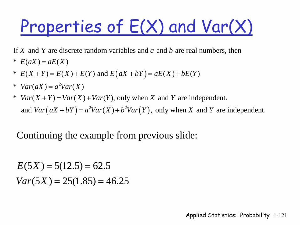
Properties of E(X) and Var(X)
( )2
If and Y are discrete random variables and and are real numbers, then* ( ) ( )* ( ) ( ) ( ) and ( ) ( )
* ( ) ( )* ( ) ( ) ( ), only when and are i
X a bE aX aE XE X Y E X E Y E aX bY aE X bE Y
Var aX a Var XVar X Y Var X Var Y X Y
=
+ = + + = +
=+ = +
( ) ( )2 2
ndependent. and ( ) , only when and are independent.Var aX bY a Var X b Var Y X Y+ = +
Continuing the example from previous slide:
(5 ) 5(12.5) 62.5(5 ) 25(1.85) 46.25
E XVar X
= == =

Applied Statistics: Probability 1-122
Expected Value vs AverageSuppose we take 10 playing cards numbered Ace, 2,3,4,5,6,7,8,9,10 and arrangethem randomly, face-down, on a table. If we choose one at random (and then replaceand reshuffle), it is equally likely that we get any value between 1 and 10. If the random variable gives the value obtained, then has a discrete uniform distributionon the integers 1 through 10. If we were asked, "What is the average
V V
( ) ( ) ( )1 1 110 10 10
face value of1+2+3+4+5+6+7+8+9+10these 10 cards?", we would compute 5.5. If we're
10asked "What is the expected value of ?", we find 1 2 10 5.5.In fact, for any random variable with dis
V
=
+ + + =
crete uniform distribution (like our "die")the expected value is the same as the average of all possible values. This is NOT TRUE for other distributions.
If we actually perform the experiment by drawing 10 times, we are not likely to get each value exactly once. For example, we might draw 1,5,2,6,8,9,7,2,3,6. The average of these outcomes is 4.9 - NOT 5.5. The more times we repeat the draw, the closer we are likely to get to the expected average of 5.5. So you might thinkof the expected value of a random variable as the value expected from averagingmany outcomes.

Applied Statistics: Probability 1-123
Binomial Mean and Variance
( )
0 1
111 1 1
0
The mean of a binomial distribution with parameter p is
( ) (1 ) (1 ) . Let 1 to get
( 1) (1 ) ( 1) (11 1 !
n nk n k k n k
k k
mnm n m m
m
n nE X k p p k p p m k
k k
n nm p p m p pm m
−−−−
− −
= =
+−+ − − +
=
⎛ ⎞ ⎛ ⎞= − = − = −⎜ ⎟ ⎜ ⎟
⎝ ⎠ ⎝ ⎠
⎛ ⎞= + − = + −⎜ ⎟+ +⎝ ⎠
∑ ∑
∑1
1
0
11
0
)
( 1) (1 ) . !
Similar work will show that Var( ) (1 ), but there are mucheasier ways to show this.
nn m
m
mnm n m
m
nnp p p npm
X np p
−− −
=
−− −
=
−= − =
= −
∑
∑
Applied Statistics: Probability 1-124
ExerciseThe interactive computer system at Gnu Glue has 20 communication lines to the central computer system. The lines operate independently and the probability that any particular line is in use is 0.6. What is the probability that 10 or more lines are in use?What is the expected number of lines in use? What is the standard deviation of lines in use?
Applied Statistics: Probability 1-125
Binomial Revisited
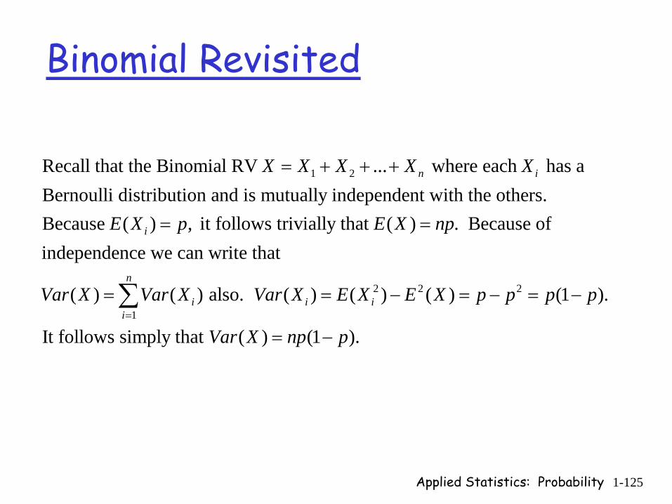
1 2Recall that the Binomial RV ... where each has a Bernoulli distribution and is mutually independent with the others. Because ( ) , it follows trivially that ( ) . Because of inde
n i
i
X X X X X
E X p E X np
= + + +
= =
2 2 2
1
pendence we can write that
( ) ( ) also. ( ) ( ) ( ) (1 ).
It follows simply that ( ) (1 ).
n
i i ii
Var X Var X Var X E X E X p p p p
Var X np p=
= = − = − = −
= −
∑

Applied Statistics: Probability 1-126
Poisson Mean and Variance
1
0 1
12 2
0 1
1
The mean of a Poisson distribution with parameter 0 is
.! ( 1)!
Similarly, ( )! ( 1)!
[ ( 1)( 1
k k
k k
k k
k k
k
ek e e ek k
eE X k e kk k
e kk
λλ λ λ
λλ
λ
λ
λ λλ λ λ
λ λλ
λλ
− −∞ ∞− −
= =
− −∞ ∞−
= =
−−
>
= = =−
= =−
= −−
∑ ∑
∑ ∑1
1 k=1
2 12 2
2 k=1
2 2 2 2
])! ( 1)!
.( 2)! ( 1)!
It follows that Var( ) ( ) ( ) .: The mean and variance of the Poisson random vari
k
k
k k
k
k
e ek k
X E X E XNOTE
λ λ
λ
λ λλ λ λ λ
λ λ λ λ
−∞ ∞
=
− −∞ ∞− −
=
+−
= + = +− −
= − = + − =
∑ ∑
∑ ∑
able, is .tX tλ
Applied Statistics: Probability 1-127
ExerciseSuppose it has been determined that the number of inquiries that arrive per second at the central computer system can be described by a Poisson random variable with an average rate of 10 messages per second. What is the probability that no inquiries arrive in a 1-second period? What is the probability that 15 or fewer inquiries arrive in a 1-second period? What are the mean and variance of the number of arrivals in 1 second?

Applied Statistics: Probability 1-128
Geometric Mean and Variance
1 1
1 1
12
0 1
2
2
( ) (1 ) (1 ) .
1 1Write ( ) (1 ) . Then ( ) (1 ) .
1 1Thus, ( ) .
(1 )Homework: Use similar technique to show that ( ) .
k k
k k
k k
k k
E X kp p p k p
s p p s p k pp p
E X pp p
pVar Xp
∞ ∞− −
= =
∞ ∞−
= =
= − = −
′= − = = − − = −
⎛ ⎞= =⎜ ⎟
⎝ ⎠−
=
∑ ∑
∑ ∑
Applied Statistics: Probability 1-129
Discrete Uniform Distribution
( )
( ) ( )( )( )
( )( )
1 1
22 2
1 1
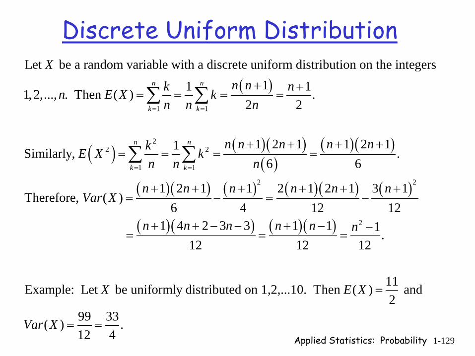
Let be a random variable with a discrete uniform distribution on the integers11 11, 2,..., . Then ( ) .
2 2
1 2 1 1 2 11Similarly, .6 6
Therefore, (
n n
k k
n n
k k
Xn nk nn E X k
n n n
n n n n nkE X kn n n
Var X
= =
= =
+ += = = =
+ + + += = = =
∑ ∑
∑ ∑
( )( ) ( ) ( )( ) ( )
( )( ) ( )( )
2 2
2
1 2 1 1 2 1 2 1 3 1)
6 4 12 121 4 2 3 3 1 1 1 .
12 12 12
11Example: Let be uniformly distributed on 1,2,...10. Then ( ) and 2
99 33( ) .12 4
n n n n n n
n n n n n n
X E X
Var X
+ + + + + += − = −
+ + − − + − −= = =
=
= =
Applied Statistics: Probability 1-130
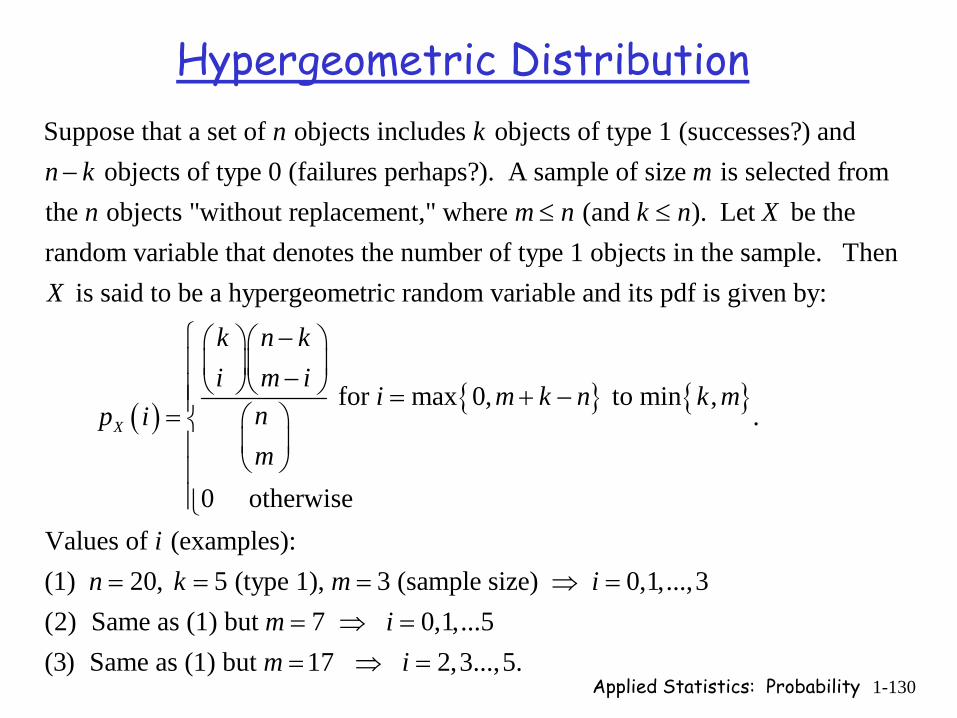
Hypergeometric DistributionSuppose that a set of objects includes objects of type 1 (successes?) and
objects of type 0 (failures perhaps?). A sample of size is selected fromthe objects "without replacement," where
n kn k m
n−
( )
(and ). Let be therandom variable that denotes the number of type 1 objects in the sample. Then
is said to be a hypergeometric random variable and its pdf is given by:
X
m n k n X
X
ki
p i
≤ ≤
⎛ ⎞⎜ ⎟⎝ ⎠
={ } { } for max 0, to min ,
.
0 otherwiseValues of (examples):(1) 20, 5 (type 1), 3 (sample size) 0,1,...,3(2) Same as (1) but 7 0,1,...5(3) Same a
n km i
i m k n k mnm
in k m i
m i
⎧ −⎛ ⎞⎪ ⎜ ⎟−⎝ ⎠⎪ = + −⎪
⎛ ⎞⎨⎜ ⎟⎪ ⎝ ⎠⎪
⎪⎩
= = = ⇒ == ⇒ =
s (1) but 17 2,3...,5.m i= ⇒ =

Applied Statistics: Probability 1-131
Text problem 3-101A company employs 800 men under the age of 55. Suppose that 30% carry a markeron the male chromosome that indicates an increased risk for high blood pressure. (a) If 10 men in the company are tested for the marker in this chromosome, what is the probability that exactly 1 man has the marker?
Answer: Notice that this is certainly sampling without replacement. (We don'tput the first man back into the pool before we draw the second one.) Let bethe number of men that have the marker in a sample of size 10. is hypergeo-
240 5601 9
metric. Thus, (1) 0.12.80010
X
XX
p
⎛ ⎞⎛ ⎞⎜ ⎟⎜ ⎟⎝ ⎠⎝ ⎠= =
⎛ ⎞⎜ ⎟⎝ ⎠

Applied Statistics: Probability 1-132
Text problem 3-101 Continued(b) If 10 men are tested for the marker, what is the probability that more than 1 has the marker?
Answer: Out of 10 the number with the marker can be 0,1,2,...,10 (because
a total of 240 have th
10 1
2 0
240 56010
0,1,...,10800e marker). Thus, ( )10
0 otherwise.
The answer is either ( ) or 1 ( ) 0.852.
X
X Xi i
i ii
p i
p i p i= =
⎧⎛ ⎞⎛ ⎞⎪⎜ ⎟⎜ ⎟−⎝ ⎠⎝ ⎠⎪ =⎪= ⎛ ⎞⎨
⎜ ⎟⎪ ⎝ ⎠⎪⎪⎩
− =∑ ∑
Applied Statistics: Probability 1-133
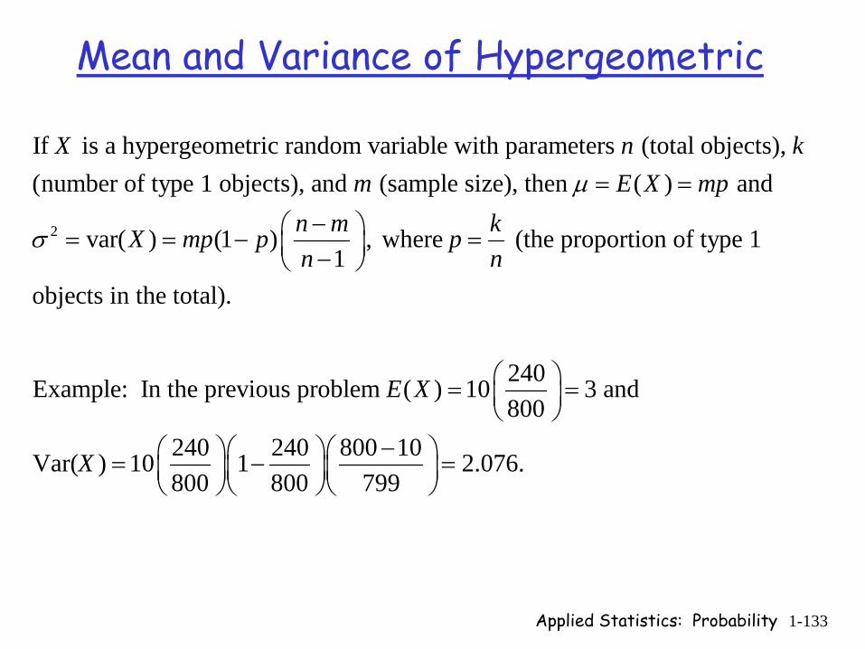
Mean and Variance of Hypergeometric
2
If is a hypergeometric random variable with parameters (total objects), (number of type 1 objects), and (sample size), then ( ) and
var( ) (1 ) , where (the proporti1
X n km E X mp
n m kX mp p pn n
μ
σ
= =
−⎛ ⎞= = − =⎜ ⎟−⎝ ⎠on of type 1
objects in the total).
240Example: In the previous problem ( ) 10 3 and800
240 240 800 10Var( ) 10 1 2.076.800 800 799
E X
X
⎛ ⎞= =⎜ ⎟⎝ ⎠
−⎛ ⎞⎛ ⎞⎛ ⎞= − =⎜ ⎟⎜ ⎟⎜ ⎟⎝ ⎠⎝ ⎠⎝ ⎠
Applied Statistics: Probability 1-134
Continuous Random Variables and Moments of Random Variables
G. A. MarinFor educational purposes only. No further distribution authorized.
Applied Statistics: Probability 1-135
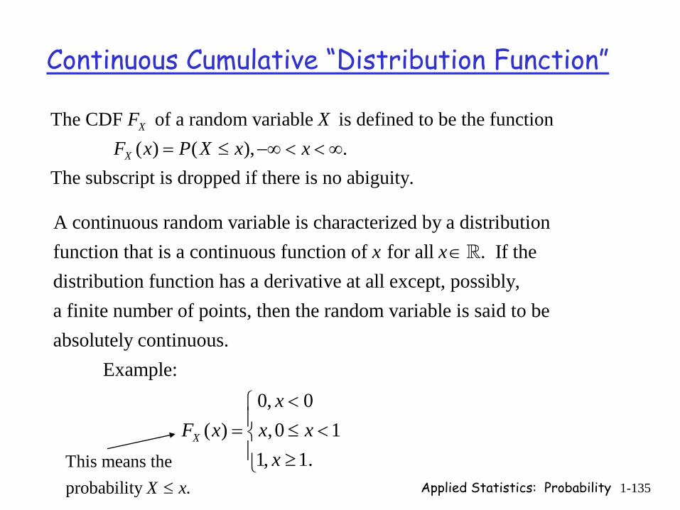
Continuous Cumulative “Distribution Function”
The CDF of a random variable is defined to be the function ( ) ( ), .The subscript is dropped if there is no abiguity.
X
X
F XF x P X x x= ≤ −∞ < < ∞
A continuous random variable is characterized by a distribution function that is a continuous function of for all . If the distribution function has a derivative at all except, possibly, a finit
x x ∈
e number of points, then the random variable is said to beabsolutely continuous. Example:
0, 0 ( ) ,0 1
1, 1.X
xF x x x
x
<⎧⎪= ≤ <⎨⎪ ≥⎩This means the
probability .X x≤
Applied Statistics: Probability 1-136
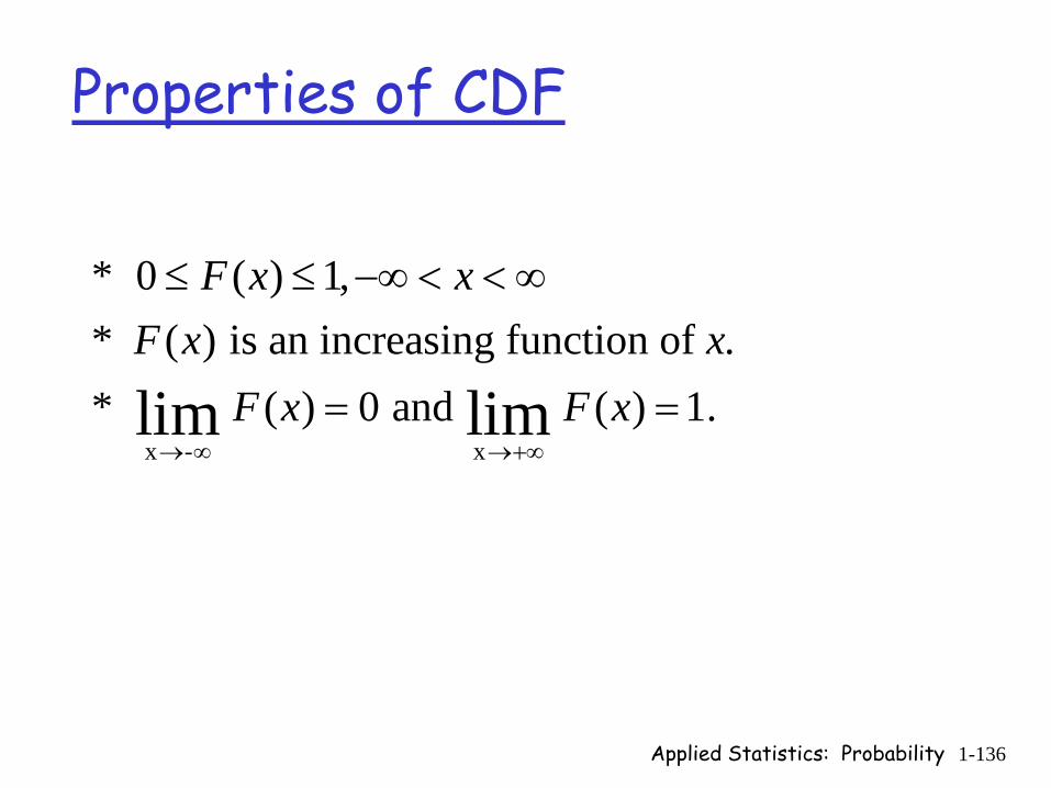
Properties of CDF
x - x
* 0 ( ) 1,* ( ) is an increasing function of .* ( ) 0 and ( ) 1.lim lim
F x xF x x
F x F x→ ∞ →+∞
≤ ≤ −∞ < < ∞
= =
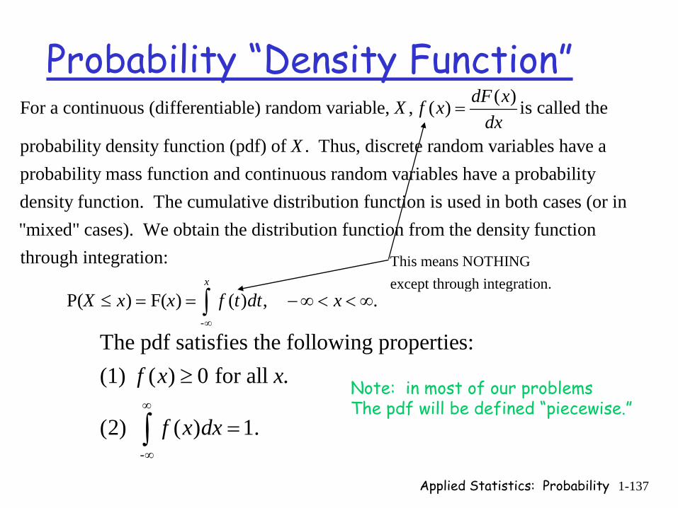
Applied Statistics: Probability 1-137
Probability “Density Function”( )For a continuous (differentiable) random variable, , ( ) is called the
probability density function (pdf) of . Thus, discrete random variables have a probability mass function and continuous
dF xX f xdx
X
=
random variables have a probability density function. The cumulative distribution function is used in both cases (or in "mixed" cases). We obtain the distribution function from the density function
-
through integration:
P( ) F( ) ( ) , .x
X x x f t dt x∞
≤ = = − ∞ < < ∞∫
-
The pdf satisfies the following properties:(1) ( ) 0 for all .
(2) ( ) 1.
f x x
f x dx∞
∞
≥
=∫Note: in most of our problemsThe pdf will be defined “piecewise.”
This means NOTHINGexcept through integration.
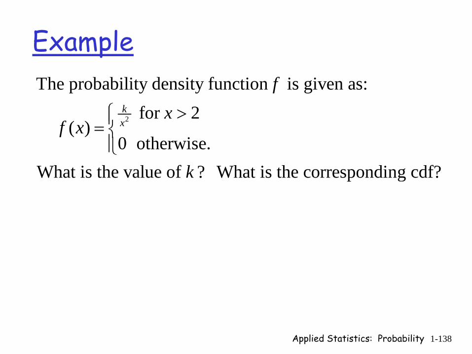
Applied Statistics: Probability 1-138
Example
2
The probability density function is given as: for 2
( )0 otherwise.
What is the value of ? What is the corresponding cdf?
kx
fx
f x
k
>⎧⎪= ⎨⎪⎩
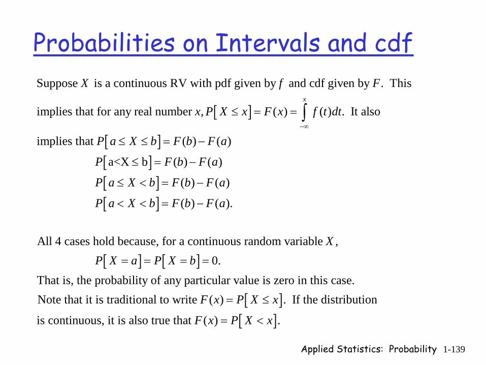
Applied Statistics: Probability 1-139
Probabilities on Intervals and cdf
[ ]
[ ][ ]
Suppose is a continuous RV with pdf given by and cdf given by . This
implies that for any real number , ( ) ( ) . It also
implies that ( ) ( )
a<X b ( )
x
X f F
x P X x F x f t dt
P a X b F b F a
P F b
−∞
≤ = =
≤ ≤ = −
≤ = −
∫
[ ][ ]
[ ] [ ]
( )
( ) ( )
( ) ( ).
All 4 cases hold because, for a continuous random variable , 0.That is, the probability of any p
F a
P a X b F b F a
P a X b F b F a
XP X a P X b
≤ < = −
< < = −
= = = =
[ ][ ]
articular value is zero in this case.Note that it is traditional to write ( ) . If the distribution
is continuous, it is also true that ( ) .
F x P X x
F x P X x
= ≤
= <

Applied Statistics: Probability 1-140
Exponential DistributionA random variable has an exponential distribution if for some >0 its distribution function is given by:
1 , if 0( )
0 otherwise.It follows that its pdf is given by:
,( )
x
x
e xF x
ef x
λ
λ
λ
λ
−
−
⎧ − ≤ < ∞= ⎨
⎩
= if 0
0 otherwise.x⎧ ≥
⎨⎩
Examples of use:• Interarrival times at a communication switch• Service times at a server• Time to failure or repair of a component.
Note that in most problems the parameter represents a "rate," such as a rate of arrivals or a rate of failures.
λ

Applied Statistics: Probability 1-141
Exponential pdf 2λ =
, if 0( )
0 otherwise.
xe xf x
λλ −⎧ ≥= ⎨
⎩
Note the values of pdf mean “nothing” except through integration.

Applied Statistics: Probability 1-142
Exponential cdf
2λ =
1 , if 0( )
0 otherwise.
xe xF x
λ−⎧ − ≤ < ∞= ⎨
⎩
Applied Statistics: Probability 1-143
Class ProblemSuppose that we stand at a mile marker on I-4 and watch cars pass. We noticethat on the average 10 cars pass by us per minute and we're given that the timelapse between two consecutive cars has an exponential distribution. If we begintiming at the moment that one car passes by, what is the probability that we will have to wait more than 20 secs for the next car to pass?
Answer. Let be waiting W
103
1 1time in minutes. We seek 1 ( ),3 3
where ( ) 1 , is the exponential cdf. The average "rate" is =10;
1thus, the answer is 0.0363
t
P W F
F t e
P W e
λ λ−
−
⎡ ⎤> = −⎢ ⎥⎣ ⎦= −
⎡ ⎤> = =⎢ ⎥⎣ ⎦
Note 20 sec = 1/3 min.
Applied Statistics: Probability 1-144
Simple Exercises
Use F in the previous problem to write:Probability W<6Probability W>6Probability W<0Probability W<-1Probability 2<W<5Probability W=1.
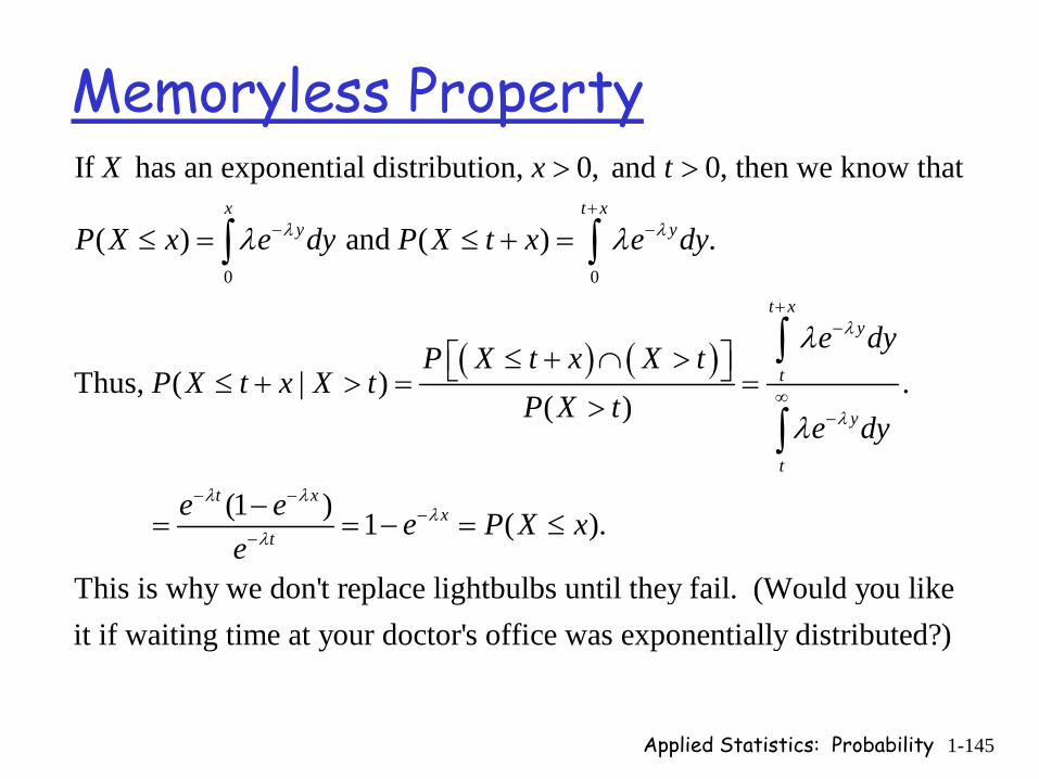
Applied Statistics: Probability 1-145
Memoryless Property
( ) ( )
0 0
If has an exponential distribution, 0, and 0, then we know that
( ) and ( ) .
Thus, ( | ) .( )
(1 )
x t xy y
t xy
t
y
t
t x
X x t
P X x e dy P X t x e dy
e dyP X t x X t
P X t x X tP X t
e dy
e ee
λ λ
λ
λ
λ λ
λ λ
λ
λ
+− −
+−
∞−
− −
−
> >
≤ = ≤ + =
≤ + ∩ >⎡ ⎤⎣ ⎦≤ + > = =>
−=
∫ ∫
∫
∫
1 ( ).
This is why we don't replace lightbulbs until they fail. (Would you likeit if waiting time at your doctor's office was exponentially distributed?)
xt e P X xλ
λ−= − = ≤
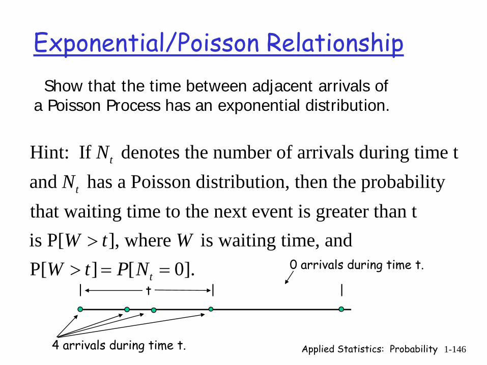
Applied Statistics: Probability 1-146
Exponential/Poisson RelationshipShow that the time between adjacent arrivals of
a Poisson Process has an exponential distribution.
Hint: If denotes the number of arrivals during time tand has a Poisson distribution, then the probability that waiting time to the next event is greater than t is P[ ], where is waiting tim
t
t
NN
W t W> e, and P[ ] [ 0].tW t P N> = =
4 arrivals during time t.
| | |
0 arrivals during time t.
t
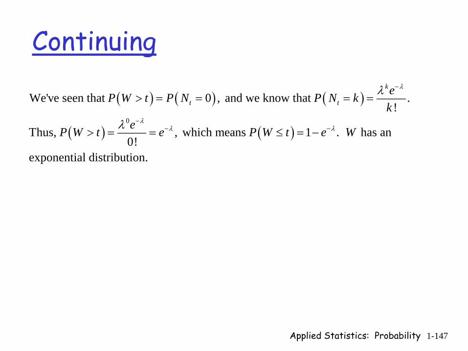
Continuing
Applied Statistics: Probability 1-147
( ) ( ) ( )
( ) ( )0
We've seen that 0 , and we know that .!
Thus, , which means 1 . has an0!
exponential distribution.
k
t teP W t P N P N kk
eP W t e P W t e W
λ
λλ λ
λ
λ
−
−− −
> = = = =
> = = ≤ = −
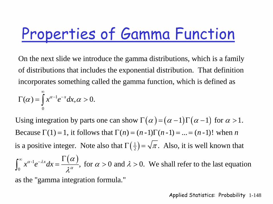
Applied Statistics: Probability 1-148
Properties of Gamma Function
( ) ( ) ( )
( )12
Using integration by parts one can show 1 1 for 1.Because (1) 1, it follows that ( ) ( -1) ( -1) ... ( -1)! when
is a positive integer. Note also that . Also, it is well known that
n n n n nα α α α
π
Γ = − Γ − >
Γ = Γ = Γ = =
Γ =
( )-1
0, for 0 and 0. We shall refer to the last equation
as the "gamma integration formula."
xx e dxα λα
αα λ
λ∞ − Γ
= > >∫
On the next slide we introduce the gamma distributions, which is a familyof distributions that includes the exponential distribution. That definitionincorporates something called the gamma function,
1
0
which is defined as
( ) , 0.xx e dxαα α∞
− −Γ = >∫

Applied Statistics: Probability 1-149
Example
( )
( )
2 4
0
1
0
2 430
Evaluate .
Answer: Recall that , for >0 and 0.
In this case -1 2 3 while =4. It follows that3 2! 1 .
4 64 32
x
x
x
x e dx
x e dx
x e dx
α λα
αλ α
λα α λ
∞ −
∞ − −
∞ −
Γ= >
= ⇒ =
Γ= = =
∫
∫
∫

Applied Statistics: Probability 1-150
Gamma DistributionA random variable with pdf given by
1
( ) , 0, 0, 0( )
tt ef t tα α λλ α λ
α
− −
= > > >Γ
Is said to have a Gamma distribution with parameters and and we write GAM( , ).Xλ α λ α∼
The parameter is called the shape parameter and the parameter is called the scale parameter. For =1 the gamma becomes
identical to the exponential distribution. NOTE: If a sequence of random var
αλ α
1 2iables , ,..., are mutually independent and identically distributed as GAM( , ), then their sum has a GAM( , ) distribution.
kX X X
kλ α
λ α
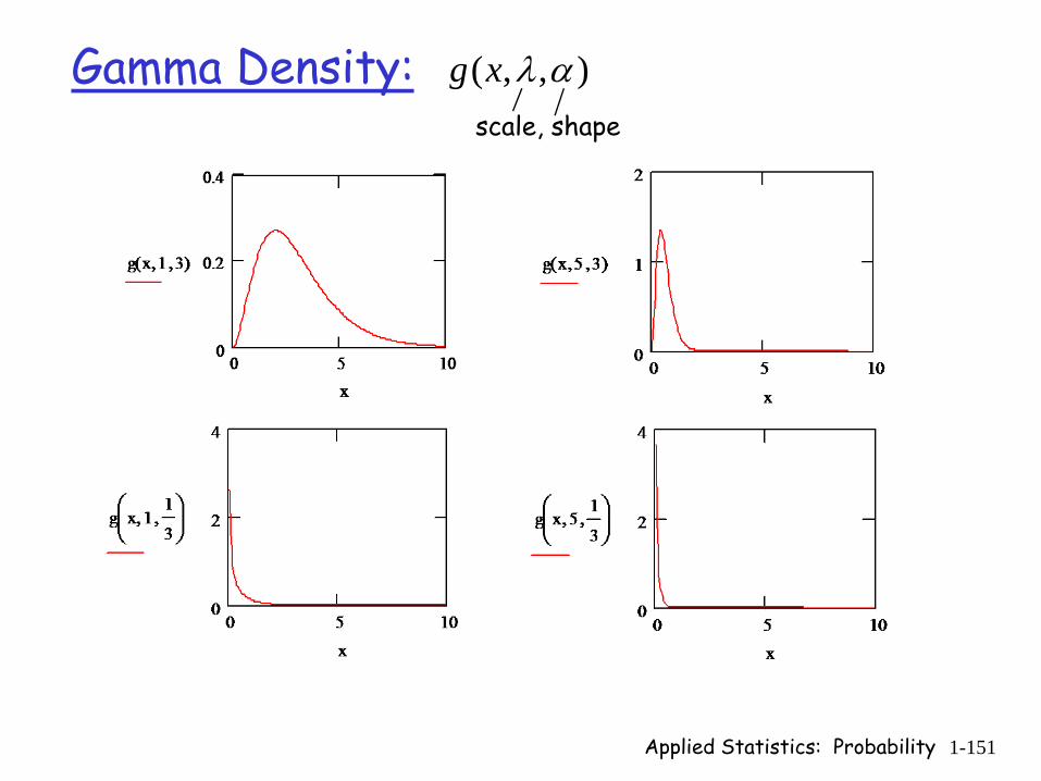
Applied Statistics: Probability 1-151
Gamma Density: ( , , )g x λ αscale, shape
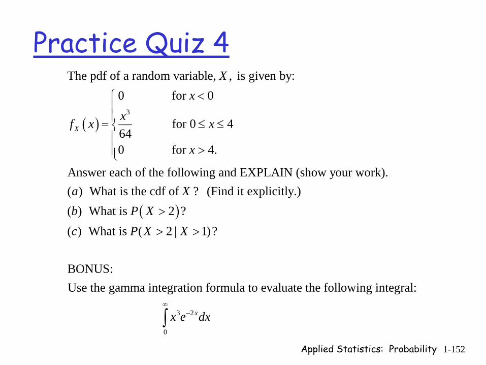
Applied Statistics: Probability 1-152
Practice Quiz 4
( )3
The pdf of a random variable, , is given by:0 for 0
for 0 4640 for 4.
Answer each of the following and EXPLAIN (show your work). ( ) What is
X
Xx
xf x x
x
a
<⎧⎪⎪= ≤ ≤⎨⎪
>⎪⎩
( )
3 2
0
the cdf of ? (Find it explicitly.)( ) What is 2 ?( ) What is ( 2 | 1)?
BONUS:Use the gamma integration formula to evaluate the following integral:
x
Xb P Xc P X X
x e dx∞
−
>
> >
∫
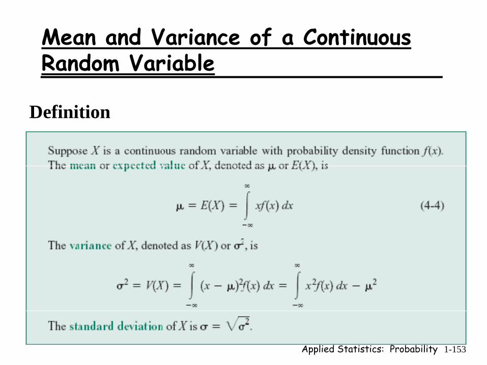
Applied Statistics: Probability 1-153
Mean and Variance of a Continuous Random Variable
Definition

Applied Statistics: Probability 1-154
Expected Value (continuous example)
( )
( )
( )
3
4 3 5
04 3 6
2 2 2
0
0 for 0
Let for 0 4 By definition 640 for 4.
4 1024 16( ) .064 5 64 5 64 5
4 4096( )064 6 64 6
X
X
X
xxf x x
x
x xE X xf x dx x dx
x xE X x f x dx x dx
∞
−∞
∞
−∞
<⎧⎪⎪= ≤ ≤⎨⎪
>⎪⎩
= = = = =× ×
= = = =× ×
∫ ∫
∫ ∫
i
i
( ) ( ) ( )2
22
3264 3
32 16 0.4273 5
Var X E X E X
=
⎛ ⎞= − = − =⎡ ⎤ ⎜ ⎟⎣ ⎦ ⎝ ⎠

Applied Statistics: Probability 1-155
Existence of E(X)
22
2 22 2
Continuing a previous example: Let be a random variable with pdf given by: for 2
( )0 otherwise.
2 2Notice that ( ) 2 ln .
Thus, well-defi
x
Xx
f x
E X x dx dx xx x
∞ ∞∞
>⎧⎪= ⎨⎪⎩
= = = = ∞∫ ∫ned random variables may not have finite means. Similarly,
a random variable may have a finite mean and not have a finite 2nd moment or a finite moment (to be defined). kth
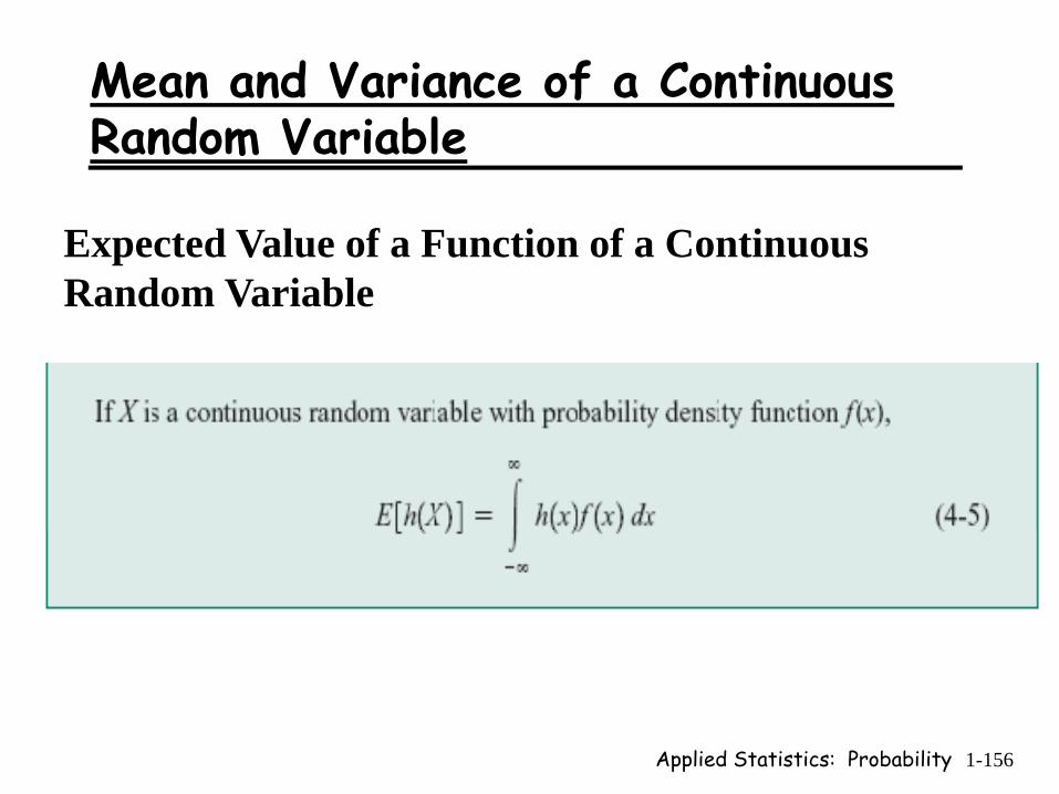
Applied Statistics: Probability 1-156
Mean and Variance of a Continuous Random Variable
Expected Value of a Function of a Continuous Random Variable
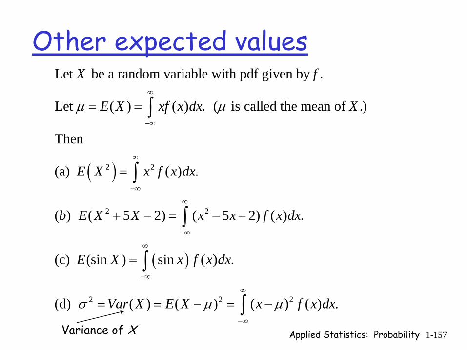
Applied Statistics: Probability 1-157
Other expected values
( )
( )
2 2
2 2
2
Let be a random variable with pdf given by .
Let ( ) ( ) . ( is called the mean of .)
Then
(a) ( ) .
( ) ( 5 2) ( 5 2) ( ) .
(c) (sin ) sin ( ) .
(d)
X f
E X xf x dx X
E X x f x dx
b E X X x x f x dx
E X x f x dx
μ μ
σ
∞
−∞
∞
−∞
∞
−∞
∞
−∞
= =
=
+ − = − −
=
∫
∫
∫
∫
2 2( ) ( ) ( ) ( ) . Var X E X x f x dxμ μ∞
−∞
= = − = −∫Variance of X
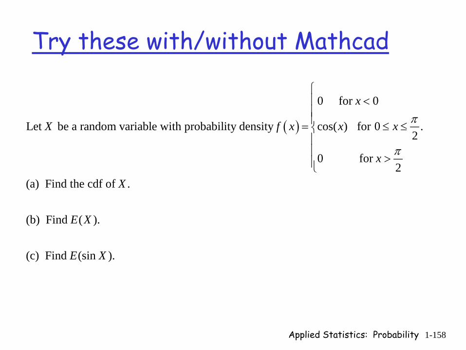
Applied Statistics: Probability 1-158
Try these with/without Mathcad
( )
0 for 0
Let be a random variable with probability density cos( ) for 0 .2
0 for 2
(a) Find the cdf of .
(b) Find ( ).
(c) Find (sin ).
x
X f x x x
x
X
E X
E X
π
π
⎧⎪ <⎪⎪= ≤ ≤⎨⎪⎪ >⎪⎩
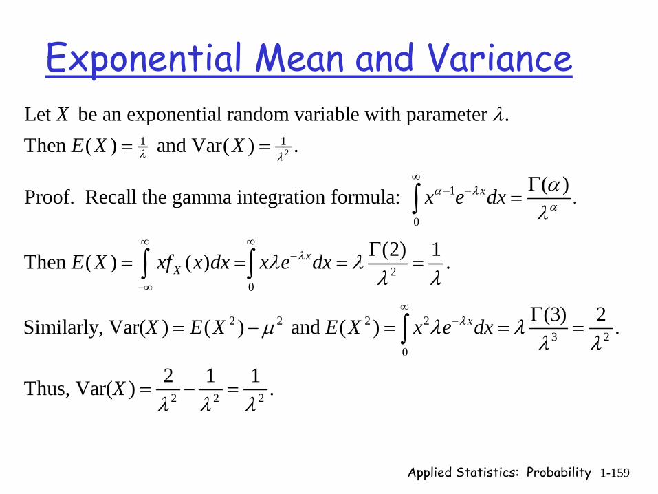
Applied Statistics: Probability 1-159
Exponential Mean and Variance
21 1
1
0
20
Let be an exponential random variable with parameter . Then ( ) and Var( ) .
( )Proof. Recall the gamma integration formula: .
(2) 1Then ( ) ( )
x
xX
XE X X
x e dx
E X xf x dx x e dx
λ λ
α λα
λ
λ
αλ
λ λλ λ
∞− −
∞ ∞−
−∞
= =
Γ=
Γ= = = =
∫
∫ ∫
2 2 2 23 2
0
2 2 2
.
(3) 2Similarly, Var( ) ( ) and ( ) .
2 1 1Thus, Var( ) .
xX E X E X x e dx
X
λμ λ λλ λ
λ λ λ
∞− Γ
= − = = =
= − =
∫
Applied Statistics: Probability 1-160
Exponential ExampleThe lifetime of a particular brand of lightbulb is exponentially distributed.The "mean time to failure" (MTTF) is 2000 hours. If the lightbulb is installedat time 0, what is the probability that it = t fails at time 3000 hours? Whatis the probability that it fails in fewer than 3000 hours?
t =

Applied Statistics: Probability 1-161
Gamma Mean and VarianceRecall that the pdf of a Gamma random variable is given by: 1
( ) , 0, 0( )
tt ef t tα α λλ α
α
− −
= > >Γ
2
The expected value (mean) of a Gamma random variable is .
The variance is .
αλ
αλ
Note that when =1, the distribution is exponential.α
Think scale**shape
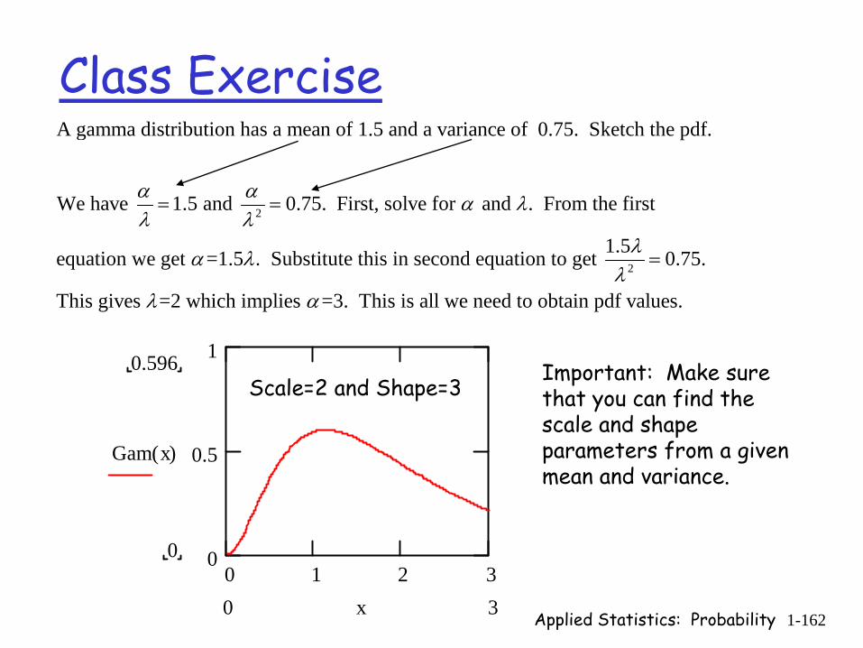
Applied Statistics: Probability 1-162
Class Exercise
2
A gamma distribution has a mean of 1.5 and a variance of 0.75. Sketch the pdf.
We have 1.5 and 0.75. First, solve for and . From the first
equation we get =1.5 . Substitute this in seco
α α α λλ λ
α λ
= =
2
1.5nd equation to get 0.75.
This gives =2 which implies =3. This is all we need to obtain pdf values.
λλ
λ α
=
Scale=2 and Shape=3
0 1 2 30
0.5
10.596
0
Gam x( )
30 x
Important: Make sure that you can find the scale and shape parameters from a given mean and variance.

Applied Statistics: Probability 1-163
Continuous Uniform DistributionA continuous random variable is said to have a uniform distributionover the interval (a,b) if its density is given by:
1 , ( )
0, otherwise.The distribution function is:
(
X
a x bf x b a
F x
⎧ < <⎪= −⎨⎪⎩
0,
) , ,
1, .
x ax a a x bb a
x b
<⎧⎪ −⎪= ≤ <⎨ −⎪
≥⎪⎩
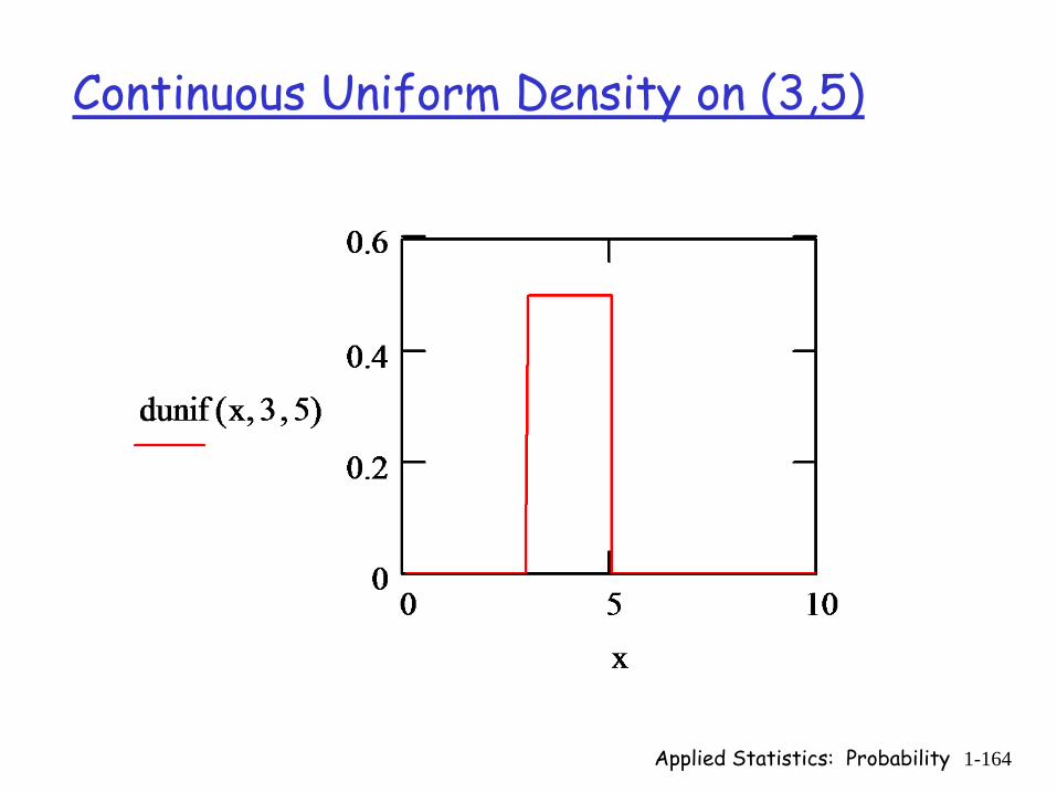
Applied Statistics: Probability 1-164
Continuous Uniform Density on (3,5)
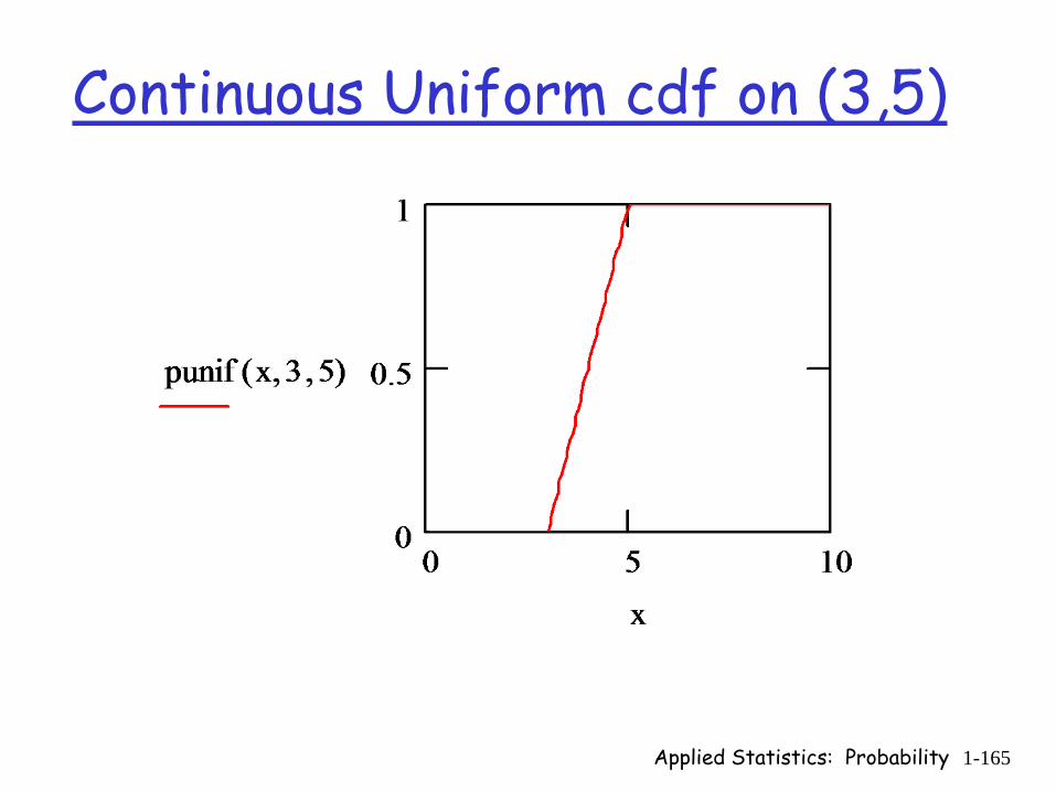
Applied Statistics: Probability 1-165
Continuous Uniform cdf on (3,5)
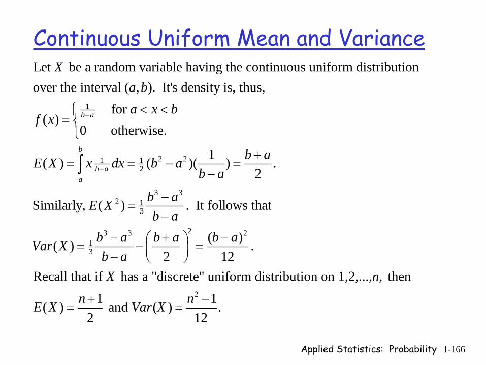
Applied Statistics: Probability 1-166
Continuous Uniform Mean and Variance
1
2 21 12
Let be a random variable having the continuous uniform distributionover the interval ( , ). It's density is, thus,
for ( )
0 otherwise.
1( ) ( )( ) .2
Si
b a
b
b aa
Xa ba x b
f x
b aE X x dx b ab a
−
−
< <⎧= ⎨
⎩+
= = − =−∫
3 32 1
3
23 3 213
2
milarly, ( ) . It follows that
( )( ) .2 12
Recall that if has a "discrete" uniform distribution on 1,2,..., , then1 1( ) and ( ) .
2 12
b aE Xb a
b a b a b aVar Xb aX n
n nE X Var X
−=
−
− + −⎛ ⎞= − =⎜ ⎟− ⎝ ⎠
+ −= =
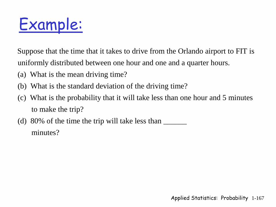
Applied Statistics: Probability 1-167
Example:Suppose that the time that it takes to drive from the Orlando airport to FIT isuniformly distributed between one hour and one and a quarter hours. (a) What is the mean driving time?(b) What is the standard deviation of the driving time?(c) What is the probability that it will take less than one hour and 5 minutes to make the trip? (d) 80% of the time the trip will take less than ______ minutes?
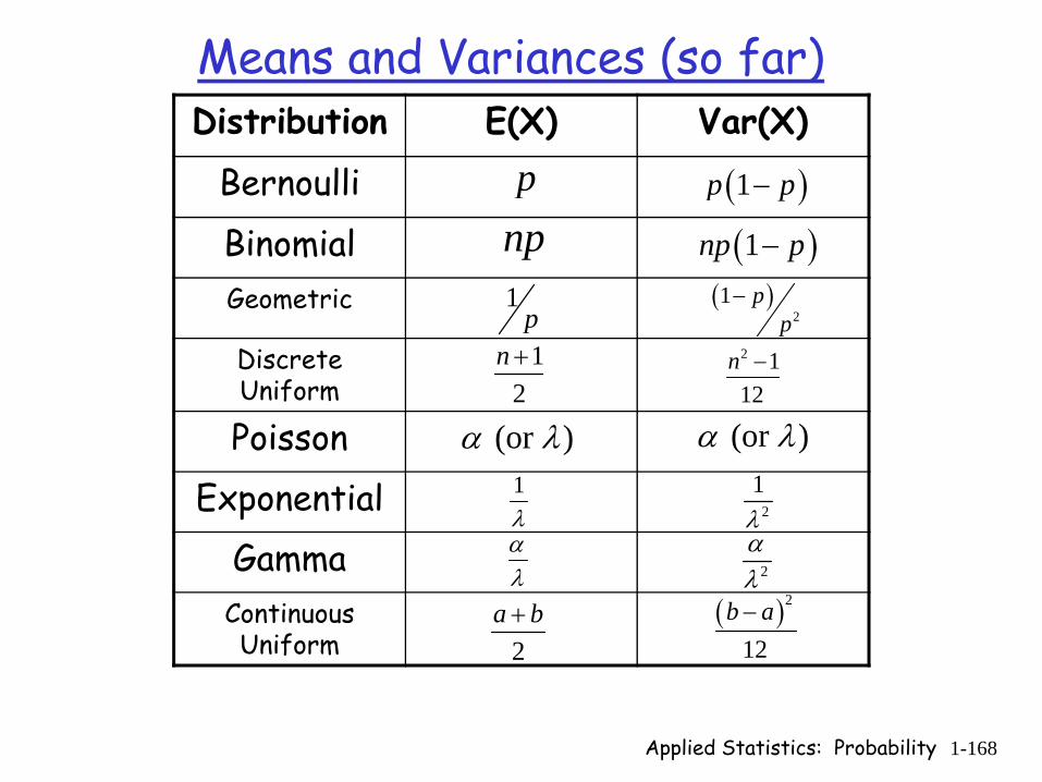
Applied Statistics: Probability 1-168
Means and Variances (so far)Distribution E(X) Var(X)
BernoulliBinomialGeometric
Discrete Uniform
PoissonExponential
GammaContinuous Uniform
p ( )1p p−
np ( )1np p−
12
n + 2 112
n −
(or )α λ (or )α λ1λ 2
1λ
αλ 2
αλ
2a b+ ( )2
12b a−
1p
( )2
1 pp
−
Applied Statistics: Probability 1-169
Practice Quiz 51. Suppose that the driving time between Orlando and Melbourne is uniformly distributed between one hour and one hour plus 15 minutes. (a) What is the variance of the driving time.? (b) Eighty percent of all drivers make the trip in fewer than minutes. What is ?2. The random variable has an exponential distribution. What is the pdf of ? What is the mean of ?
xx
X XX What is the variance of ? (Just write down what
we known the mean and variance are. Do not derive them from the definition.)3. The random variable has a Binomial distribution and the total n
X
X umber of trials is 30. (a) If the probability of success on a single trial is 0.2, write the pmf for . (b) If ( ) 2.1, then what is the probability of success on a single trial?
XE X =
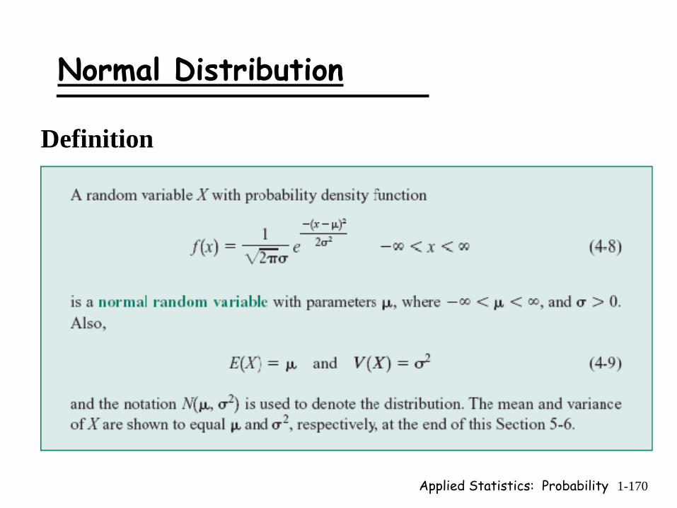
Applied Statistics: Probability 1-170
Normal Distribution
Definition
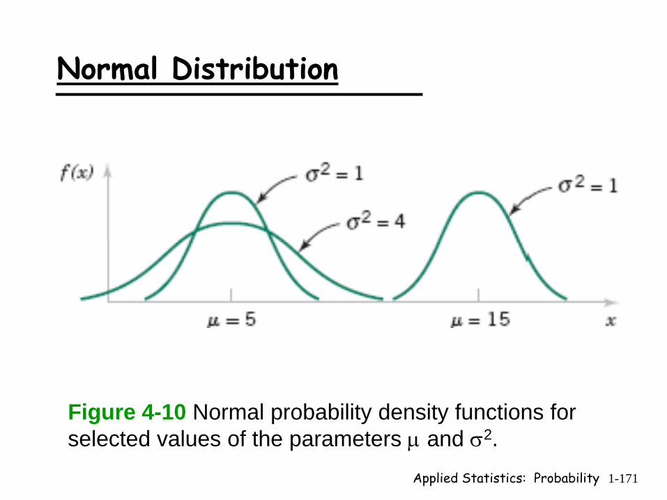
Applied Statistics: Probability 1-171
Normal Distribution
Figure 4-10 Normal probability density functions for selected values of the parameters μ and σ2.
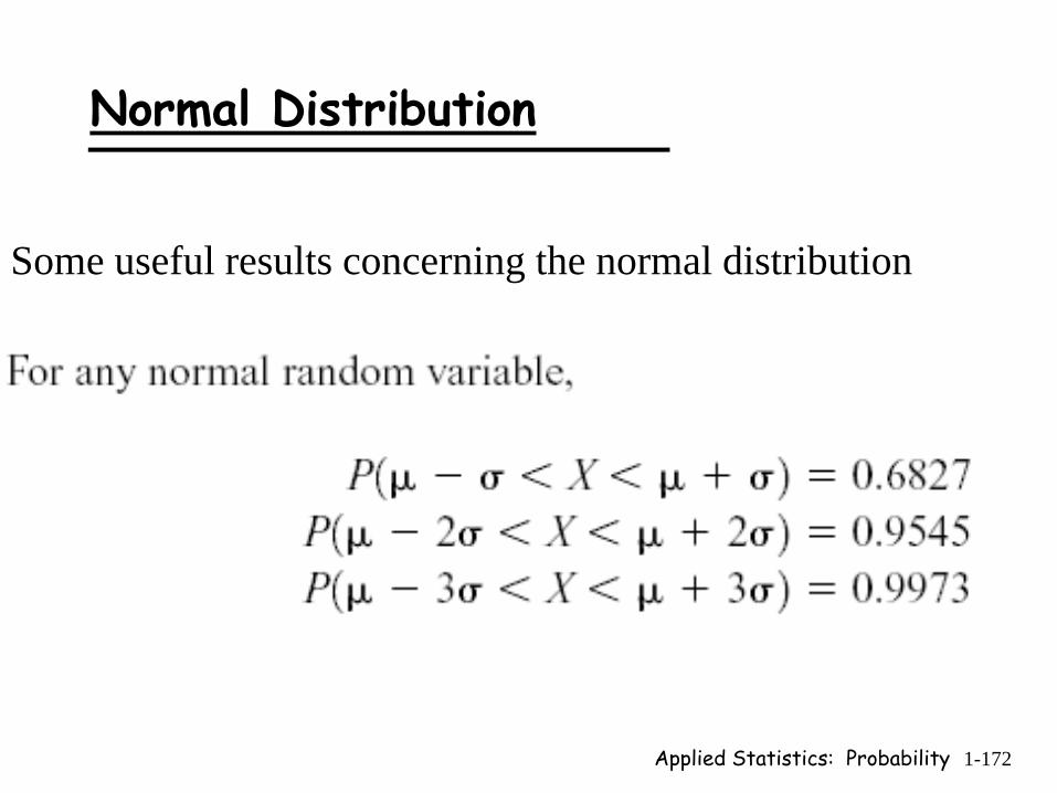
Applied Statistics: Probability 1-172
Normal Distribution
Some useful results concerning the normal distribution
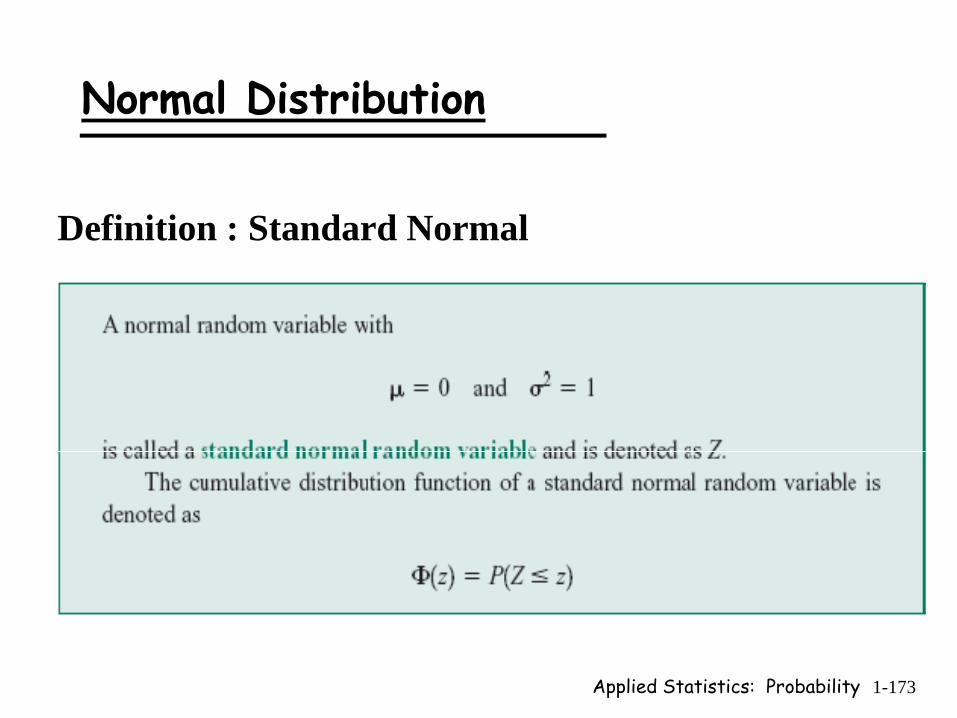
Applied Statistics: Probability 1-173
Normal Distribution
Definition : Standard Normal
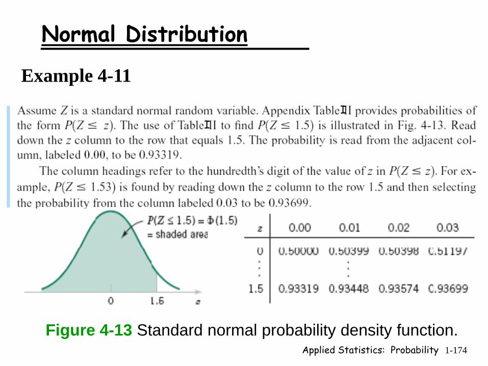
Applied Statistics: Probability 1-174
Normal Distribution
Example 4-11
Figure 4-13 Standard normal probability density function.
II

Applied Statistics: Probability 1-175
0.00 0.01 0.02 0.03 0.04 0.05 0.06 0.07 0.08 0.09
0.0 0.5000 0.5040 0.5080 0.5120 0.5160 0.5199 0.5239 0.5279 0.5319 0.5359
0.1 0.5398 0.5438 0.5478 0.5517 0.5557 0.5596 0.5636 0.5675 0.5714 0.5753
0.2 0.5793 0.5832 0.5871 0.5910 0.5948 0.5987 0.6026 0.6064 0.6103 0.6141
0.3 0.6179 0.6217 0.6255 0.6293 0.6331 0.6368 0.6406 0.6443 0.6480 0.6517
0.4 0.6554 0.6591 0.6628 0.6664 0.6700 0.6736 0.6772 0.6808 0.6844 0.6879
0.5 0.6915 0.6950 0.6985 0.7019 0.7054 0.7088 0.7123 0.7157 0.7190 0.7224
0.6 0.7257 0.7291 0.7324 0.7357 0.7389 0.7422 0.7454 0.7486 0.7517 0.7549
0.7 0.7580 0.7611 0.7642 0.7673 0.7704 0.7734 0.7764 0.7794 0.7823 0.7852
0.8 0.7881 0.7910 0.7939 0.7967 0.7995 0.8023 0.8051 0.8078 0.8106 0.8133
0.9 0.8159 0.8186 0.8212 0.8238 0.8264 0.8289 0.8315 0.8340 0.8365 0.8389
1.0 0.8413 0.8438 0.8461 0.8485 0.8508 0.8531 0.8554 0.8577 0.8599 0.8621
1.1 0.8643 0.8665 0.8686 0.8708 0.8729 0.8749 0.8770 0.8790 0.8810 0.8830
1.2 0.8849 0.8869 0.8888 0.8907 0.8925 0.8944 0.8962 0.8980 0.8997 0.9015
1.3 0.9032 0.9049 0.9066 0.9082 0.9099 0.9115 0.9131 0.9147 0.9162 0.9177
1.4 0.9192 0.9207 0.9222 0.9236 0.9251 0.9265 0.9279 0.9292 0.9306 0.9319
1.5 0.9332 0.9345 0.9357 0.9370 0.9382 0.9394 0.9406 0.9418 0.9429 0.9441
1.6 0.9452 0.9463 0.9474 0.9484 0.9495 0.9505 0.9515 0.9525 0.9535 0.9545
1.7 0.9554 0.9564 0.9573 0.9582 0.9591 0.9599 0.9608 0.9616 0.9625 0.9633
1.8 0.9641 0.9649 0.9656 0.9664 0.9671 0.9678 0.9686 0.9693 0.9699 0.9706
1.9 0.9713 0.9719 0.9726 0.9732 0.9738 0.9744 0.9750 0.9756 0.9761 0.9767
2.0 0.9772 0.9778 0.9783 0.9788 0.9793 0.9798 0.9803 0.9808 0.9812 0.9817
2.1 0.9821 0.9826 0.9830 0.9834 0.9838 0.9842 0.9846 0.9850 0.9854 0.9857
2.2 0.9861 0.9864 0.9868 0.9871 0.9875 0.9878 0.9881 0.9884 0.9887 0.9890
2.3 0.9893 0.9896 0.9898 0.9901 0.9904 0.9906 0.9909 0.9911 0.9913 0.9916
2.4 0.9918 0.9920 0.9922 0.9925 0.9927 0.9929 0.9931 0.9932 0.9934 0.9936
2.5 0.9938 0.9940 0.9941 0.9943 0.9945 0.9946 0.9948 0.9949 0.9951 0.9952
2.6 0.9953 0.9955 0.9956 0.9957 0.9959 0.9960 0.9961 0.9962 0.9963 0.9964
2.7 0.9965 0.9966 0.9967 0.9968 0.9969 0.9970 0.9971 0.9972 0.9973 0.9974
2.8 0.9974 0.9975 0.9976 0.9977 0.9977 0.9978 0.9979 0.9979 0.9980 0.9981
2.9 0.9981 0.9982 0.9982 0.9983 0.9984 0.9984 0.9985 0.9985 0.9986 0.9986
3.0 0.9987 0.9987 0.9987 0.9988 0.9988 0.9989 0.9989 0.9989 0.9990 0.9990
Standard Normal Table

Applied Statistics: Probability 1-176
Normal Distribution
Standardizing
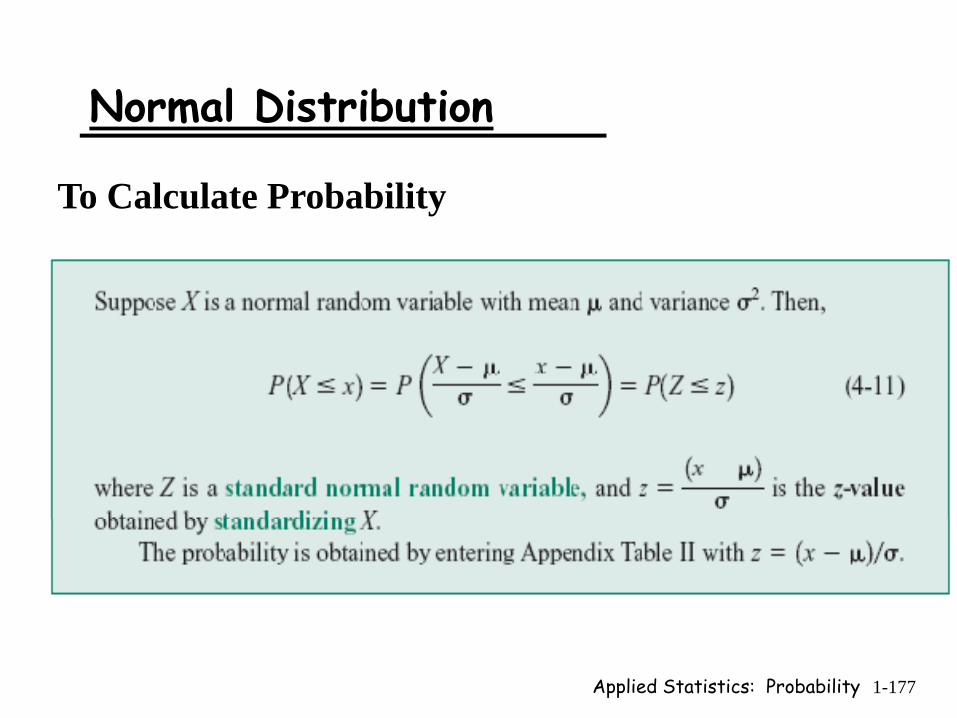
Applied Statistics: Probability 1-177
Normal Distribution
To Calculate Probability
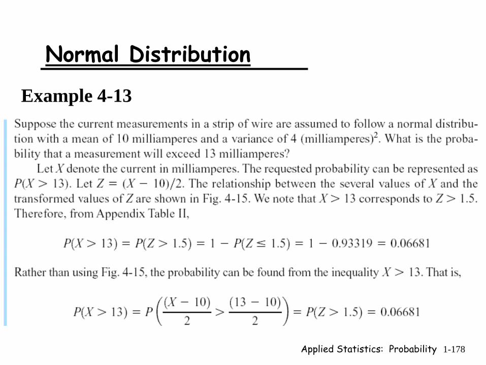
Applied Statistics: Probability 1-178
Normal Distribution
Example 4-13
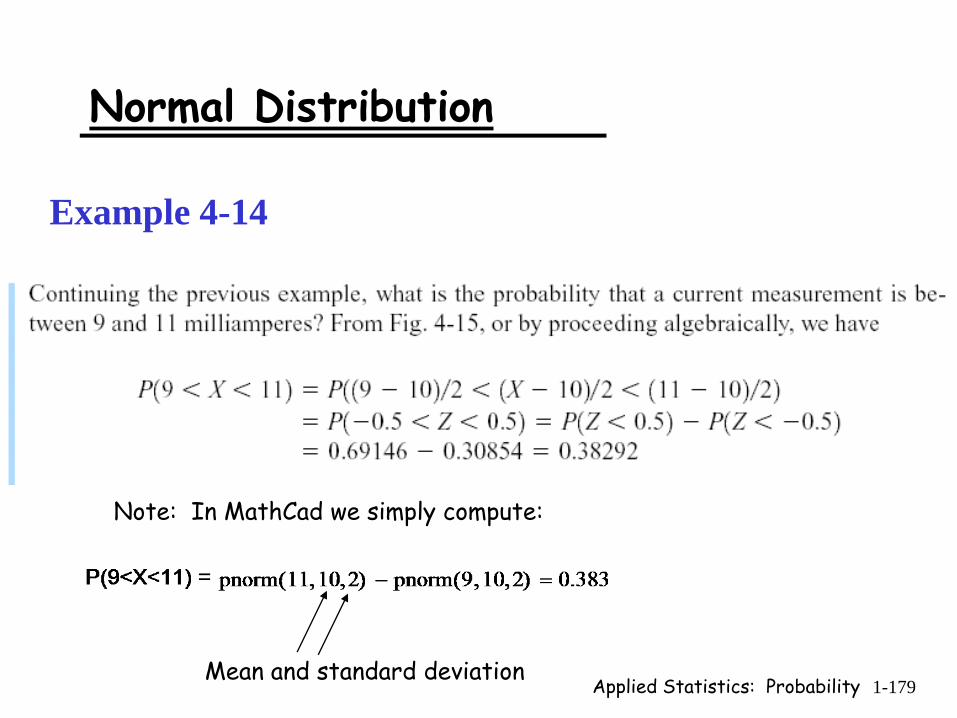
Applied Statistics: Probability 1-179
Normal Distribution
Example 4-14
Note: In MathCad we simply compute:
Mean and standard deviation
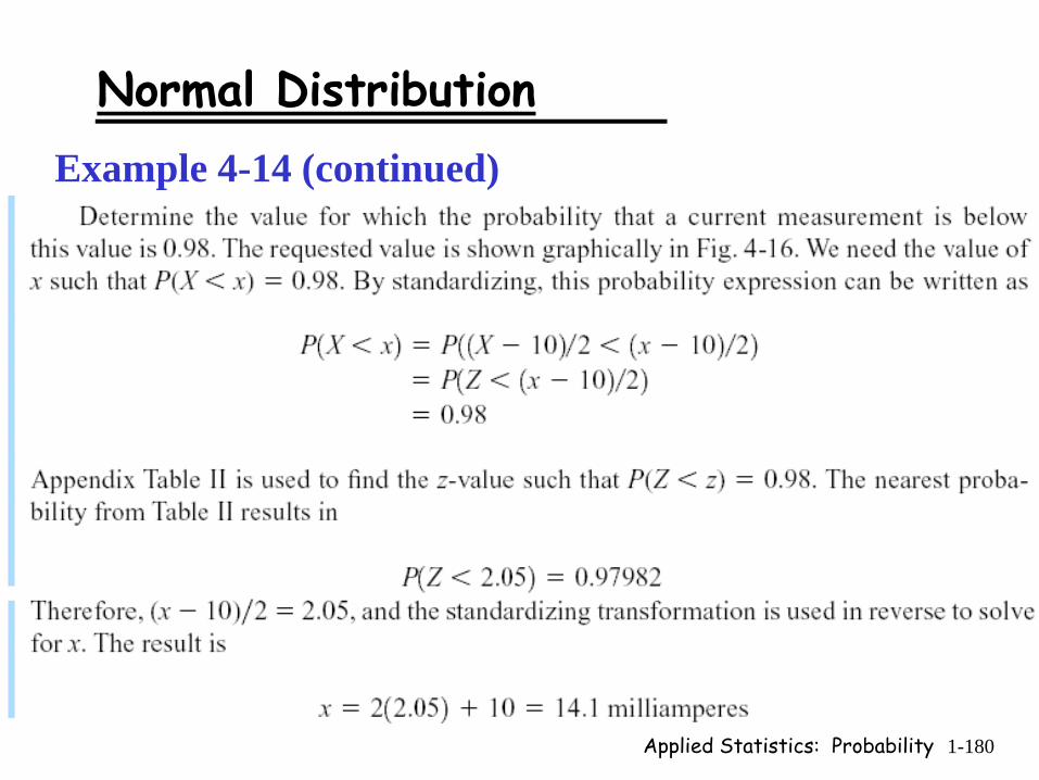
Applied Statistics: Probability 1-180
Normal DistributionExample 4-14 (continued)
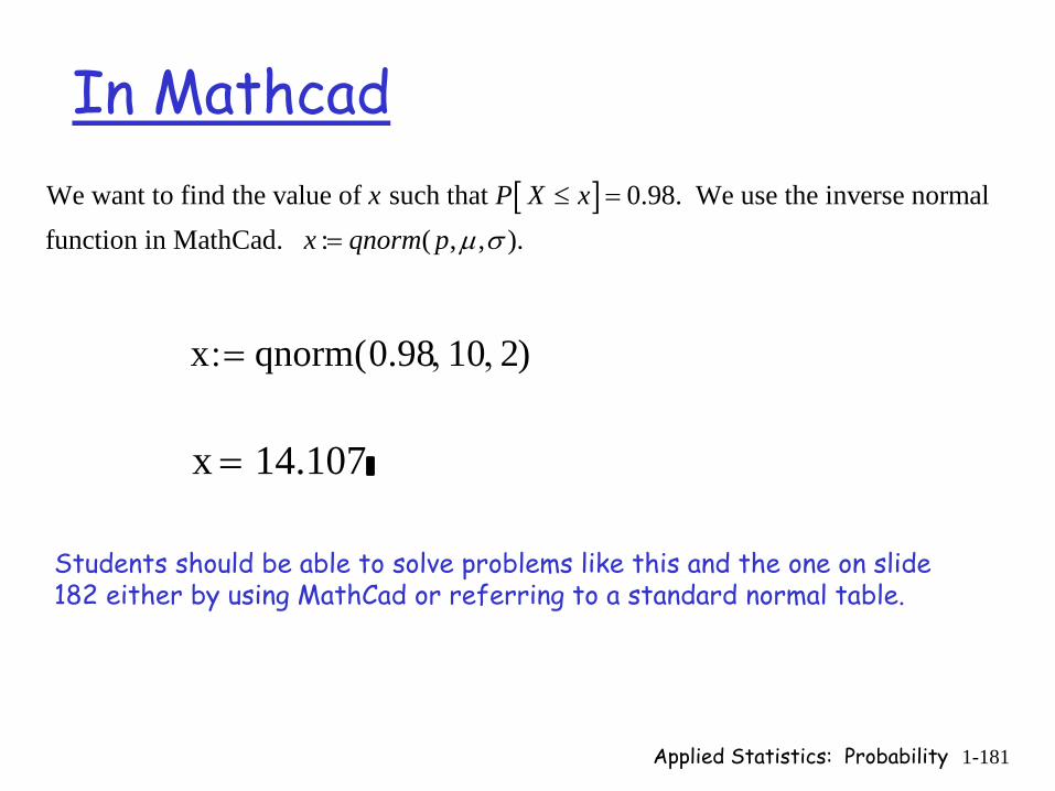
Applied Statistics: Probability 1-181
In Mathcad[ ]We want to find the value of such that 0.98. We use the inverse normal
function in MathCad. : ( , , ).x P X x
x qnorm p μ σ≤ =
=
x qnorm 0.98 10, 2, ( ):=
x 14.107=
Students should be able to solve problems like this and the one on slide 182 either by using MathCad or referring to a standard normal table.
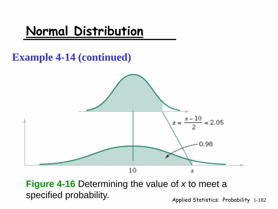
Applied Statistics: Probability 1-182
Normal Distribution
Example 4-14 (continued)
Figure 4-16 Determining the value of x to meet a specified probability.
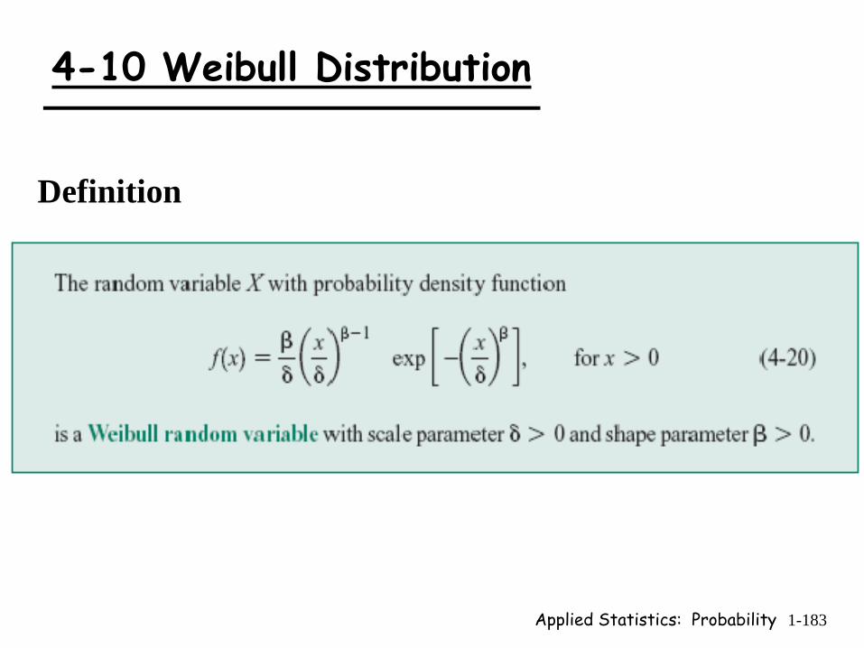
Applied Statistics: Probability 1-183
4-10 Weibull Distribution
Definition

Applied Statistics: Probability 1-184
4-10 Weibull Distribution
Figure 4-26 Weibull probability density functions for selected values of and β.δ
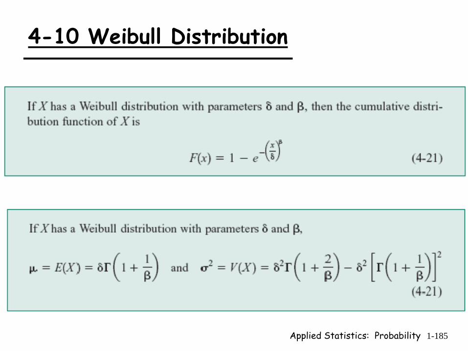
Applied Statistics: Probability 1-185
4-10 Weibull Distribution
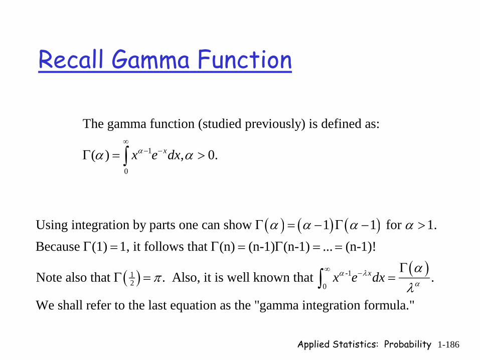
Applied Statistics: Probability 1-186
Recall Gamma Function
( ) ( ) ( )
( ) ( )-112 0
Using integration by parts one can show 1 1 for 1.Because (1) 1, it follows that (n) (n-1) (n-1) ... (n-1)!
Note also that . Also, it is well known that .
We shall ref
xx e dxα λα
α α α α
απ
λ∞ −
Γ = − Γ − >
Γ = Γ = Γ = =
ΓΓ = =∫
er to the last equation as the "gamma integration formula."
1
0
The gamma function (studied previously) is defined as:
( ) , 0.xx e dxαα α∞
− −Γ = >∫
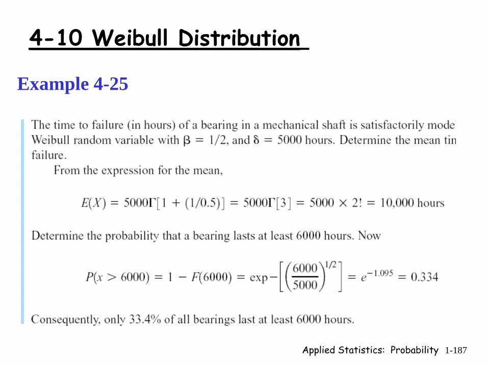
Applied Statistics: Probability 1-187
4-10 Weibull Distribution
Example 4-25

Applied Statistics: Probability 1-188
4-11 Lognormal Distribution“X is log-normal means ln(X) is normal.”

Applied Statistics: Probability 1-189
4-11 Lognormal Distribution
Figure 4-27 Lognormal probability density functions with θ = 0 for selected values of ω2.
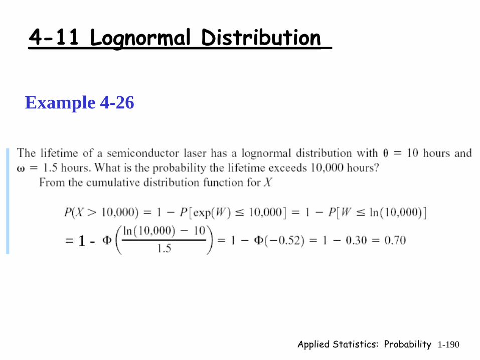
Applied Statistics: Probability 1-190
4-11 Lognormal Distribution
Example 4-26
= 1 -

Applied Statistics: Probability 1-191
4-11 Lognormal Distribution
Example 4-26 (continued)
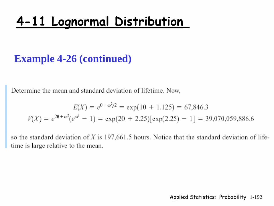
Applied Statistics: Probability 1-192
4-11 Lognormal Distribution
Example 4-26 (continued)
Applied Statistics: Probability 1-193
Joint Probability DistributionsWhen two or more random variables naturally occur together or take values thatseem to be related, it is common to consider their joint probability distributions.Suppose, for example, that and are X Y two random variables whose outcomeswe wish to consider jointly. In a manner similar to single random variables weconsider two cases. (1) and are discrete. Here we use a joint pmf and joiX Y nt cdf (tbd). (2) and are continuous. Here we use a joint pdf and joint cdf (tbd).X Y
Examples:
(1) The location of a ship is given by its latitude and longitude. Suppose you are searching for a ship from its last known position. It is natural to consider the joint distribution of ( , ), the ship's probable position.
(2) Similarly an aircraft's position might be predicted using a joint distribution of ( , , ), where ( , ) is as above and is altitude.
X Y
X Y Z X Y Z
Applied Statistics: Probability 1-194
Discrete Random Variables
1 2
1 2
, ,... 1 2
1 1 2 2
For discrete random variables , ,..., their joint probability massfunction is given by:
( ) ( , ,..., )
= ( , ,..., )
If only two random variables are involv
n
n
X X X X n
n n
X X X
p x p x x x
P X x X x X x
=
= = =
1 2
,
,
ed, we usually denote them as and Y,instead of , and , and we write:
( , ) ( , ).
Note that the author writes the latter as ( , ) ( , ).
X Y
X Y
XX X
p x y P X x Y y
f x y P X x Y y
= = =
= = =
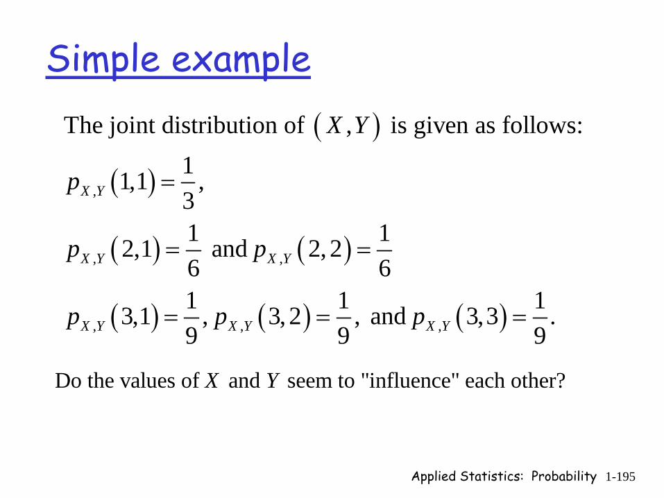
Applied Statistics: Probability 1-195
Simple example( )
( )
( ) ( )
( ) ( ) ( )
,
, ,
, , ,
The joint distribution of , is given as follows:11,1 , 31 12,1 and 2, 26 61 1 13,1 , 3,2 , and 3,3 .9 9 9
X Y
X Y X Y
X Y X Y X Y
X Y
p
p p
p p p
=
= =
= = =
Do the values of and seem to "influence" each other?X Y
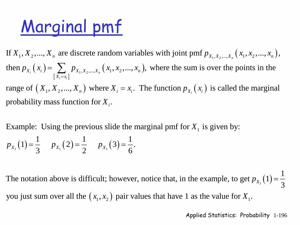
Applied Statistics: Probability 1-196
Marginal pmf( )
( ) ( )[ ]
( )
1 2
1 2
1 2 , ,..., 1 2
, ,..., 1 2
1 2
If , ,..., are discrete random variables with joint pmf , ,..., ,
then , ,..., , where the sum is over the points in the
range of , ,..., where
n
i n
i i
n X X X n
X i X X X nX x
n i
X X X p x x x
p x p x x x
X X X X=
= ∑
( )
( ) ( ) ( )1 1 1
1
. The function is called the marginal
probability mass function for .
Example: Using the previous slide the marginal pmf for is given by:1 1 11 2 3 .3 2 6
The notation abov
ii X i
i
X X X
x p x
X
X
p p p
=
= = =
( )
( )1
1 2 1
1e is difficult; however, notice that, in the example, to get 13
you just sum over all the , pair values that have 1 as the value for .
Xp
x x X
=
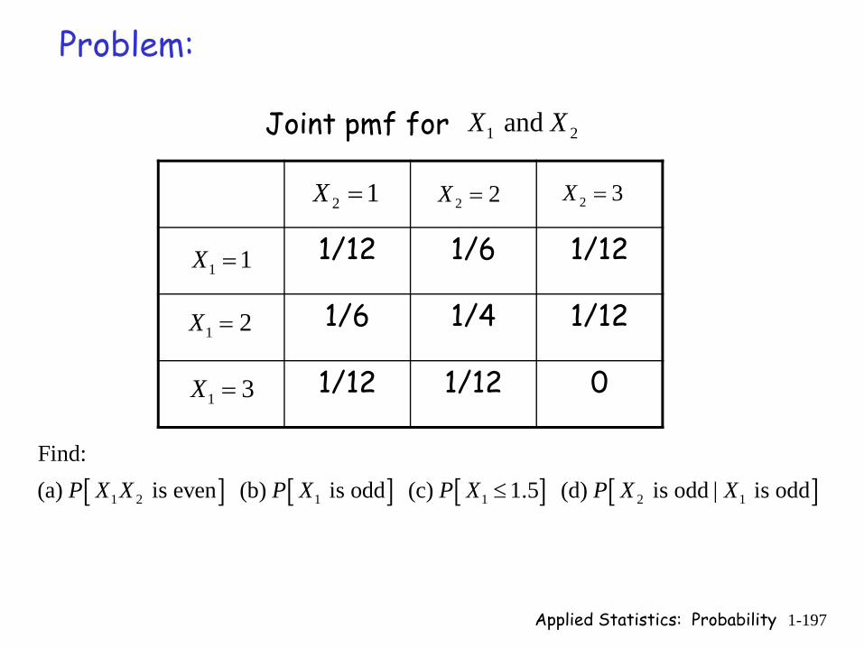
Applied Statistics: Probability 1-197
Problem:
1/12 1/6 1/12
1/6 1/4 1/12
1/12 1/12 0
Joint pmf for 1 2and X X
1 1X =
1 2X =
1 3X =
2 1X = 2 2X = 2 3X =
[ ] [ ] [ ] [ ]1 2 1 1 2 1
Find: (a) is even (b) is odd (c) 1.5 (d) is odd | is oddP X X P X P X P X X≤

Applied Statistics: Probability 1-198
Joint PMF and Independence
1 2
1 2
, ,... 1 2
1 1 2 2
For discrete random variables , ,..., their joint probability massfunction is given by:
( ) ( , ,..., )
= ( , ,..., )n
n
X X X X n
n n
X X X
p x p x x x
P X x X x X x
=
= = =
1 2
1 2
1 2
The discrete random variables , ,..., are said to be mutually independent if their joint pmf can be written as:
( ) ( ) ( ) ( ).n
n
X X X X n
X X X
p x p x p x p x= iii
1 2In the previous example are and independent?X X
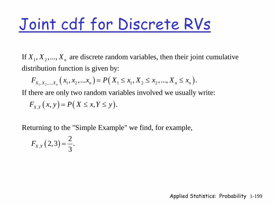
Applied Statistics: Probability 1-199
Joint cdf for Discrete RVs
( ) ( )1 2
1 2
, ,..., 1 2 1 1 2 2
If , ,..., are discrete random variables, then their joint cumulative distribution function is given by: , ,... , ,..., .
If there are only two random variablesn
n
X X X n n n
X X X
F x x x P X x X x X x= ≤ ≤ ≤
( ) ( )
( )
,
,
involved we usually write: , , .
Returning to the "Simple Example" we find, for example, 2 2,3 .3
X Y
X Y
F x y P X x Y y
F
= ≤ ≤
=
Applied Statistics: Probability 1-200
Skip Section 5-1.3
We will not cover the material on conditional probability distributions that is in this section of the text.
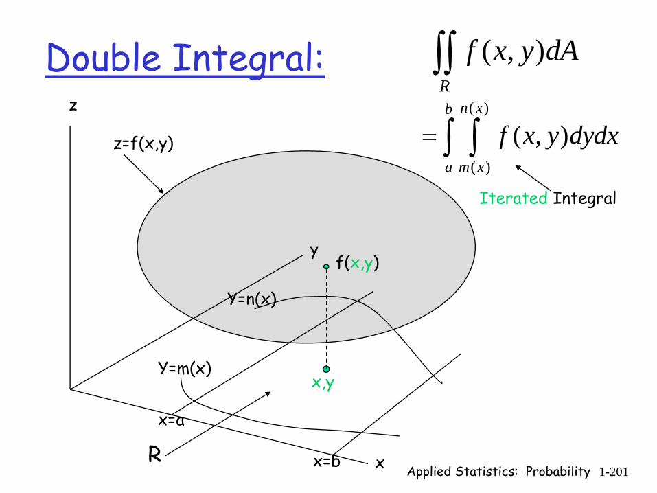
Applied Statistics: Probability 1-201
Double Integral:z
x
y
x=a
x=b
Y=n(x)
Y=m(x)x,y
z=f(x,y)
R
( , )R
f x y dA∫∫
f(x,y)
( )
( )
( , )n xb
a m x
f x y dydx= ∫ ∫Iterated Integral

Applied Statistics: Probability 1-202
Example:
2
Evaluate the double integral 2 where is the region bounded by the
curve and the lines 0 and 2.R
xydA R
y x y x= = =
∫∫
0 1 2 30
2
45
0
x2
30 x2x =
Region R
2 222 2 2
2
00 0 0 0 0
2 6 24
00
Answer: 2 2
32 .6 3
|
|
x xx
xydydx x ydydx x y dx
xxx dx
⎛ ⎞= = ⎜ ⎟⎝ ⎠
= = =
∫ ∫ ∫ ∫ ∫
∫
Computes the volume under the surface z=2xy and above the region R.
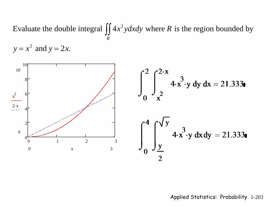
Applied Statistics: Probability 1-203
3
2
Evaluate the double integral 4 where is the region bounded by
and 2 .R
x ydxdy R
y x y x= =
∫∫
0 1 2 30
2
4
6
8
1010
0
x2
2 x⋅
30 x
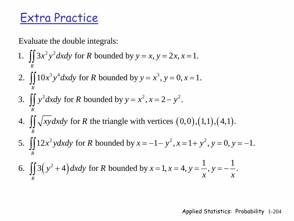
Applied Statistics: Probability 1-204
Extra Practice
2 2
3 4 3
2 2 2
Evaluate the double integrals:
1. 3 for bounded by , 2 , 1.
2. 10 for bounded by , 0, 1.
3. for bounded by , 2 .
4. for the triangle wi
R
R
R
x y dxdy R y x y x x
x y dxdy R y x y x
y dxdy R y x x y
xydxdy R
= = =
= = =
= = −
∫∫
∫∫
∫∫( ) ( ) ( )
( )
2 2 2
2
th vertices 0,0 , 1,1 , 4,1 .
5. 12 for bounded by 1 , 1 , 0, 1.
1 16. 3 4 for bounded by 1, 4, , .
R
R
R
x ydxdy R x y x y y y
y dxdy R x x y yx x
= − − = + = = −
+ = = = = −
∫∫
∫∫
∫∫
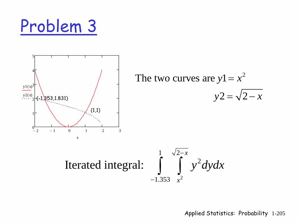
Applied Statistics: Probability 1-205
Problem 3
2− 1− 0 1 2 30
1
2
3
4
5
y1 x( )
y2 x( )
x
(1,1)
(-1.353,1.831)
2
1 22
1.353
Iterated integral: x
x
y dydx−
−∫ ∫
2The two curves are 1
2 2
y x
y x
=
= −

Applied Statistics: Probability 1-206
Joint Distribution of Continuous RVs
,
The cumulative joint distribution of continuous random variables X and Y is defined by ( , ) ( , ), , .Properties:* 0 ( , ) 1* ( , ) is monotone increasing in BOTH variables* P
X YF x y P X x Y y x y
F x yF x y
= ≤ ≤ −∞ < < ∞ −∞ < < ∞
≤ ≤
,
,
( and ) ( , ) ( , ) ( , ) ( , ) Note: ( , ) ( ) is called the marginal cumulative distribution of .
( , ) ( ) is called the marginal cumulative d
lim lim
X Y Xy
X Y Yx
a X b c Y d F b d F a d F b c F a c
F x y F x X
F x y F y→∞
→∞
< ≤ < ≤ = − − +
=
=
( ) [ ] [ ] ( ),
istribution of Y.
Think of F , .Also: The marginal cdf is defined in the same manner for discrete random variables.
X X Yx P X x P X x Y F x= ≤ = ≤ < ∞ ≈ ∞∩
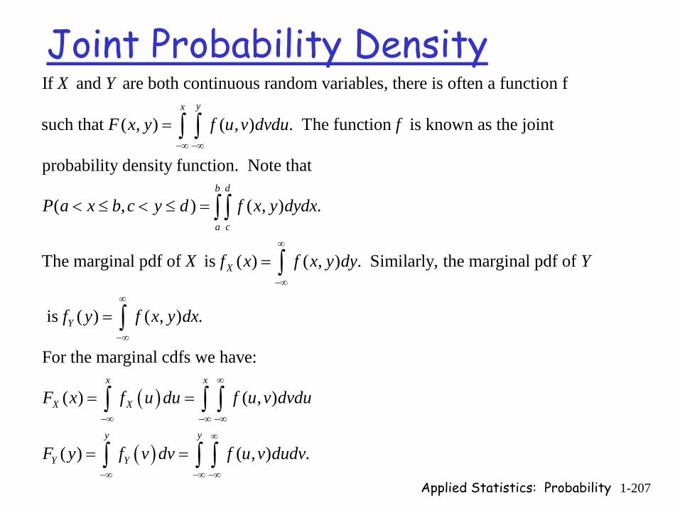
Applied Statistics: Probability 1-207
Joint Probability DensityIf and are both continuous random variables, there is often a function f
such that ( , ) ( , ) . The function is known as the joint
probability density function. Note that
( ,
yx
X Y
F x y f u v dvdu f
P a x b c
−∞ −∞
=
< ≤
∫ ∫
( )
( )
) ( , ) .
The marginal pdf of is ( ) ( , ) . Similarly, the marginal pdf of
is ( ) ( , ) .
For the marginal cdfs we have:
( ) ( , )
( )
b d
a c
X
Y
x x
X X
Y Y
y d f x y dydx
X f x f x y dy Y
f y f x y dx
F x f u du f u v dvdu
F y f v dv
∞
−∞
∞
−∞
∞
−∞ −∞ −∞
−
< ≤ =
=
=
= =
=
∫ ∫
∫
∫
∫ ∫ ∫
( , ) .y y
f u v dudv∞
∞ −∞ −∞
=∫ ∫ ∫
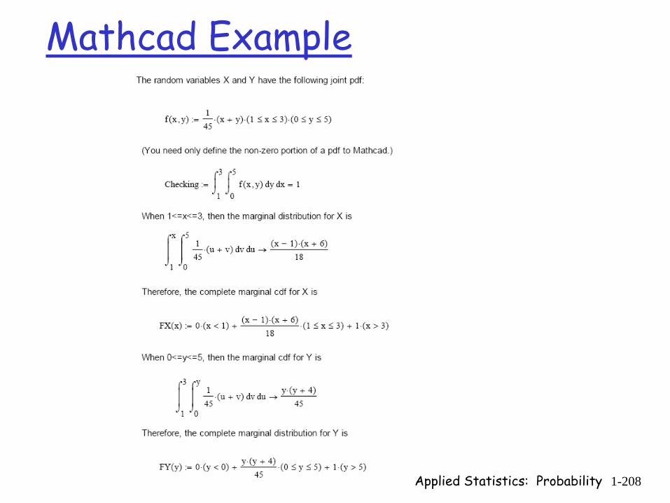
Applied Statistics: Probability 1-208
Mathcad Example
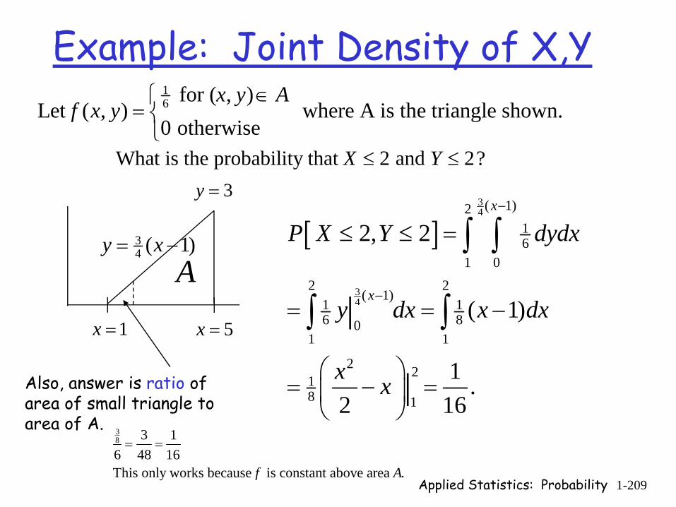
Applied Statistics: Probability 1-209
Example: Joint Density of X,Y16 for ( , )
Let ( , ) where A is the triangle shown.0 otherwise
x y Af x y
∈⎧= ⎨
⎩
1x = 5x =
3y =
What is the probability that 2 and 2?X Y≤ ≤
A[ ]
34
34
( 1)216
1 0
2 2( 1)
1 16 80
1 1
2 218 1
2, 2
( 1)
1 .2 16
|
|
x
x
P X Y dydx
y dx x dx
x x
−
−
≤ ≤ =
= = −
⎛ ⎞= − =⎜ ⎟
⎝ ⎠
∫ ∫
∫ ∫
34 ( 1)y x= −
Also, answer is ratio of area of small triangle to area of A. 3
8 3 16 48 16This only works because is constant above area .f A
= =
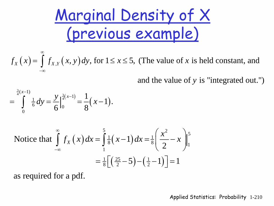
Applied Statistics: Probability 1-210
Marginal Density of X (previous example)
( ) ( )
( ) ( )34 3
4
,
( 1)1
16 0
0
, , for 1 5, (The value of is held constant, and
and the value of is "integrated out.")
1 1 .6 8|
X X Y
xx
f x f x y dy x x
y
ydy x
∞
−∞
−−
= ≤ ≤
= = = −
∫
∫
( ) ( )
( ) ( )
5 2 51 18 8 1
1
251 18 2 2
Notice that 12
5 1 1
as required for a pdf.
|Xxf x dx x dx x
∞
−∞
⎛ ⎞= − = −⎜ ⎟
⎝ ⎠⎡ ⎤= − − − =⎣ ⎦
∫ ∫

Applied Statistics: Probability 1-211
Example:
( ) ( )
2 212
The random variables and have the joint density function
exp ( ) for 0 and 0 ( , )
0 otherwise.
Find , , and (1,2).
: W
Y X
X Y
xy x y x yf x y
F y f x F
Solution
⎧ ⎡ ⎤− + > >⎪ ⎣ ⎦= ⎨⎪⎩
( )
( )2 2 2
2
2
,0
2 21 2 2 220 0
2
e begin by finding ( , ) .
exp ( ) .
By symmetry, ( ) , also. This is 's density function,
and we can now find the cdf, ( )
X X Y
x y x
X
y
Y
t
Y
f x f x y dy
f x xy x y dy xe ye dy xe
f y ye Y
F y te
∞
∞ ∞− − −
−
−
=
⎡ ⎤= − + = =⎣ ⎦
=
=
∫
∫ ∫
2 2
2 2 20
0
1 .|y t y
ydt e e
− −= − = −∫
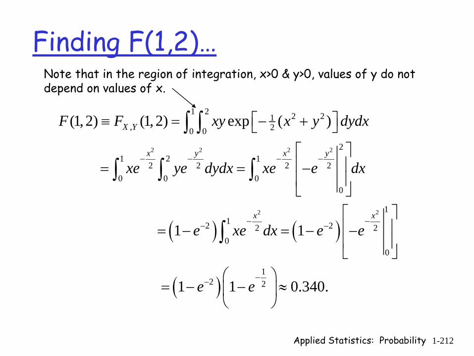
Applied Statistics: Probability 1-212
Finding F(1,2)…
( ) ( )
2 2 2 2
2 2
1 2 2 21, 20 0
21 2 1
2 2 2 20 0 0
0
112 22 20
0
(1, 2) (1, 2) exp ( )
1 1
1
X Y
x y x y
x x
F F xy x y dydx
xe ye dydx xe e dx
e xe dx e e
− − − −
− −− −
⎡ ⎤≡ = − +⎣ ⎦
⎡ ⎤⎢ ⎥= = −⎢ ⎥⎣ ⎦
⎡ ⎤⎢ ⎥= − = − −⎢ ⎥⎣ ⎦
= −
∫ ∫
∫ ∫ ∫
∫
( )1
2 21 0.340.e e−− ⎛ ⎞
− ≈⎜ ⎟⎝ ⎠
Note that in the region of integration, x>0 & y>0, values of y do not depend on values of x.
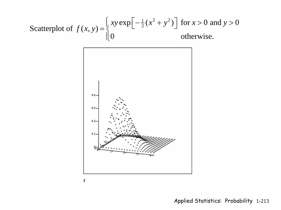
Applied Statistics: Probability 1-213
2 212exp ( ) for 0 and 0
Scatterplot of ( , )0 otherwise.
xy x y x yf x y
⎧ ⎡ ⎤− + > >⎪ ⎣ ⎦= ⎨⎪⎩
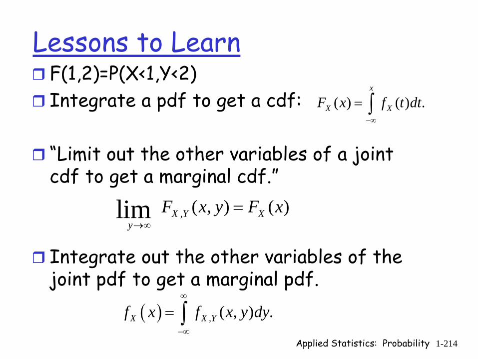
Applied Statistics: Probability 1-214
Lessons to LearnF(1,2)=P(X<1,Y<2)Integrate a pdf to get a cdf:
“Limit out the other variables of a joint cdf to get a marginal cdf.”
Integrate out the other variables of the joint pdf to get a marginal pdf.
( ) ( ) .x
X XF x f t dt−∞
= ∫
, ( , ) ( )lim X Y Xy
F x y F x→∞
=
( ) , ( , ) .X X Yf x f x y dy∞
−∞
= ∫
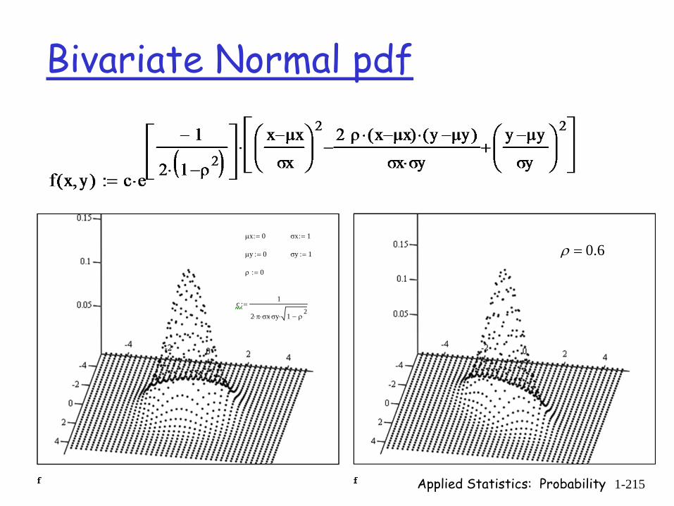
Applied Statistics: Probability 1-215
Bivariate Normal pdf
μx 0:= σx 1:=
μy 0:= σy 1:=
ρ 0:=
c1
2 π⋅ σx⋅ σy⋅ 1 ρ2
−⋅
:=
0.6ρ =
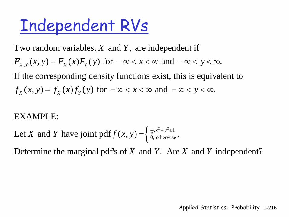
Applied Statistics: Probability 1-216
Independent RVs
,
Two random variables, and , are independent if( , ) ( ) ( ) for and .
If the corresponding density functions exist, this is equivalent to ( , ) ( ) ( ) for and
X Y X Y
X X Y
X YF x y F x F y x y
f x y f x f y x y
= − ∞ < < ∞ − ∞ < < ∞
= − ∞ < < ∞ − ∞ < < ∞
{ 2 21 , 10, otherwise
.
EXAMPLE:
Let and have joint pdf ( , ) .
Determine the marginal pdf's of and . Are and independent?
x yX Y f x y
X Y X Y
π + ≤=
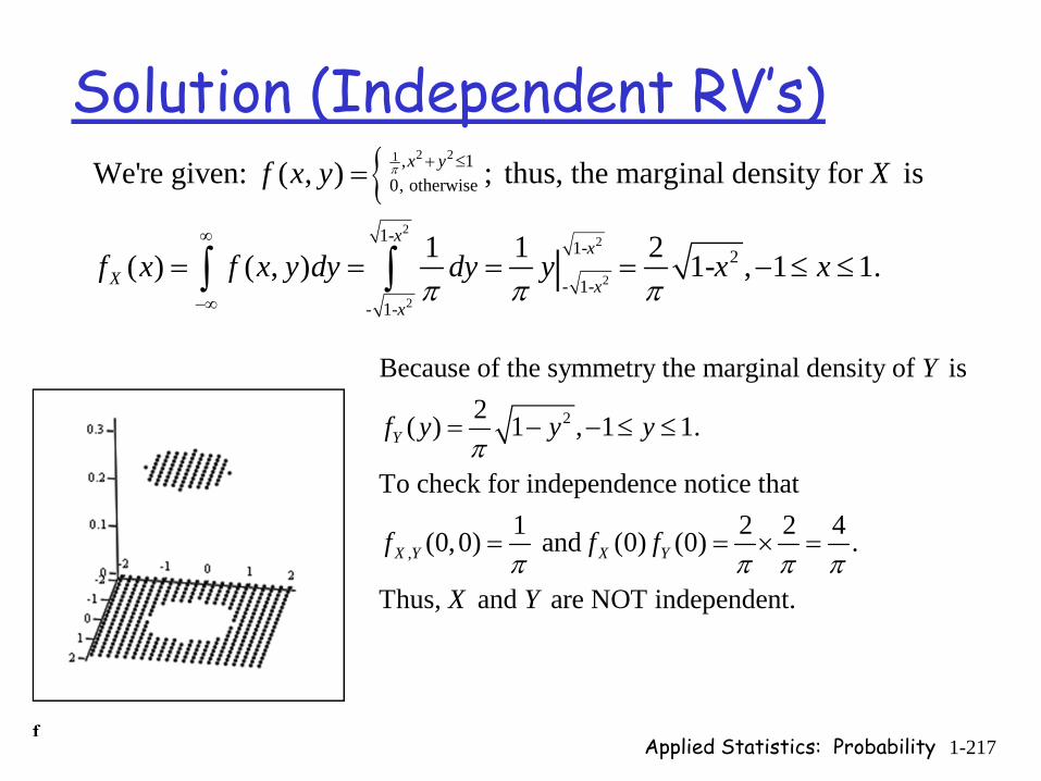
Applied Statistics: Probability 1-217
Solution (Independent RV’s){ 2 21
22
2
2
, 10, otherwise
1-1- 2
- 1-- 1-
We're given: ( , ) ; thus, the marginal density for is
1 1 2( ) ( , ) 1- , 1 1.|
x y
xx
X xx
f x y X
f x f x y dy dy y x x
π
π π π
+ ≤
∞
−∞
=
= = = = − ≤ ≤∫ ∫
2
,
Because of the symmetry the marginal density of is 2( ) 1 , 1 1.
To check for independence notice that 1 2 2 4(0,0) and (0) (0) .
Thus, and are NOT independent.
Y
X Y X Y
Y
f y y y
f f f
X Y
π
π π π π
= − − ≤ ≤
= = × =
Applied Statistics: Probability 1-218
Sums of Independent Normals1, 2
n
1
2 2
1 1
Let ,..., be independent random variables with distributions
given by ( , ), then ( , )
where = and . Note that the Avg of the random
variables will have mea
n
i i i ii
n n
i ii i
X X X
X N X N
n
μ σ μ σ
μ μ σ σ
=
= =
=
∑
∑ ∑
∼ ∼
n and standard deviation = .n nμ σ
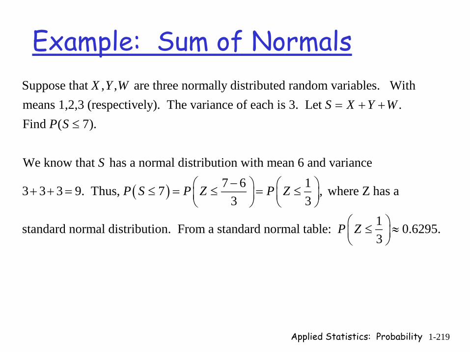
Applied Statistics: Probability 1-219
Example: Sum of NormalsSuppose that , , are three normally distributed random variables. Withmeans 1,2,3 (respectively). The variance of each is 3. Let .Find ( 7).
We know that has a normal distribution with
X Y WS X Y W
P S
S
= + +≤
( )
mean 6 and variance 7 6 13 3 3 9. Thus, 7 , where Z has a
3 31standard normal distribution. From a standard normal table: 0.6295.3
P S P Z P Z
P Z
−⎛ ⎞ ⎛ ⎞+ + = ≤ = ≤ = ≤⎜ ⎟ ⎜ ⎟⎝ ⎠ ⎝ ⎠
⎛ ⎞≤ ≈⎜ ⎟⎝ ⎠
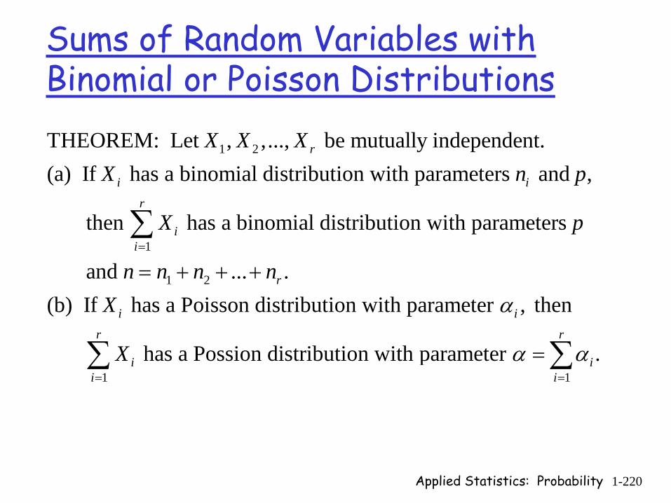
Applied Statistics: Probability 1-220
Sums of Random Variables with Binomial or Poisson Distributions
1 2
1
1 2
THEOREM: Let , ,..., be mutually independent.(a) If has a binomial distribution with parameters and ,
then has a binomial distribution with parameters
and .
r
i ir
ii
X X XX n p
X p
n n n=
= + +
∑
1 1
.. .(b) If has a Poisson distribution with parameter , then
has a Possion distribution with parameter .
r
i i
r r
i ii i
nX
X
α
α α= =
+
=∑ ∑

Applied Statistics: Probability 1-221
Keeping Sums in the Family
A sum of independent normals is normal.A sum of independent Poissons is Poisson.A sum of independent exponentials is Erlang.A sum of independent gammas is gamma.A large sum of independent, identically distributed RVs is approximately normal.

Applied Statistics: Probability 1-222
Erlang Distribution
1
When sequential phases have identical exponential distributions, thenthe resulting density is known as an -stage Erlang and is given by:
( ) , for 0, 0, 1, 2,....( 1)!
The di
r r t
rr
t ef t t rr
λλ λ− −
= > > =−
1
0
stribution function is given by:( ) ( ) 1 0, 0, 1, 2,....
! Note that the exponential is a special case of the Erlang distribution with 1. One may also think of this
krt
k
tF t e t rk
r
λλ λ−
−
=
= − ≥ > =
=
∑
as the distribution function for the sum ofr mutually independent random variables each with the exponential distributionwith parameter .λ
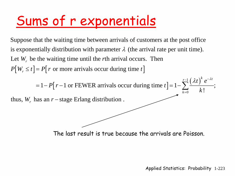
Applied Statistics: Probability 1-223
Sums of r exponentialsSuppose that the waiting time between arrivals of customers at the post officeis exponentially distribution with parameter (the arrival rate per unit time). Let be the waiting time until the th rW r
λ
[ ] [ ]
[ ] ( )1
0
arrival occurs. Then or more arrivals occur during time
1 1 or FEWER arrivals occur during time 1 ;!
thus, has an stage Erlang distribution .
r
k tr
k
r
P W t P r t
t eP r t
kW r
λλ −−
=
≤ =
= − − = −
−
∑
The last result is true because the arrivals are Poisson.
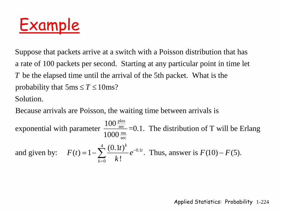
Applied Statistics: Probability 1-224
ExampleSuppose that packets arrive at a switch with a Poisson distribution that has a rate of 100 packets per second. Starting at any particular point in time let
be the elapsed time until the arrival of tT
pktssec
mssec
he 5th packet. What is the probability that 5ms 10ms?Solution.Because arrivals are Poisson, the waiting time between arrivals is
100exponential with parameter =0.1. The distributio1000
T≤ ≤
40.1
0
n of T will be Erlang
(0.1 )and given by: ( ) 1 . Thus, answer is (10) (5).!
kt
k
tF t e F Fk
−
=
= − −∑
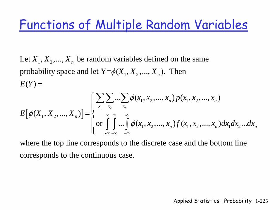
Applied Statistics: Probability 1-225
Functions of Multiple Random Variables
[ ]1 2
1 2
1 2
1 2 1 2
1 2
1 2
Let , ,..., be random variables defined on the same probability space and let Y= ( , ,..., ). Then
( )
... ( , ,..., ) ( , ,..., )
( , ,..., )or ... ( , ,..., )
n
n
n
n nx x x
n
n
X X XX X X
E Y
x x x p x x x
E X X Xx x x
φ
φ
φφ
∞ ∞
−∞ −∞
=
=
∑∑ ∑
∫ ∫ 1 2 1 2-
( , ,..., ) ...
where the top line corresponds to the discrete case and the bottom linecorresponds to the continuous case.
n nf x x x dx dx dx∞
∞
⎧⎪⎪⎨⎪⎪⎩
∫
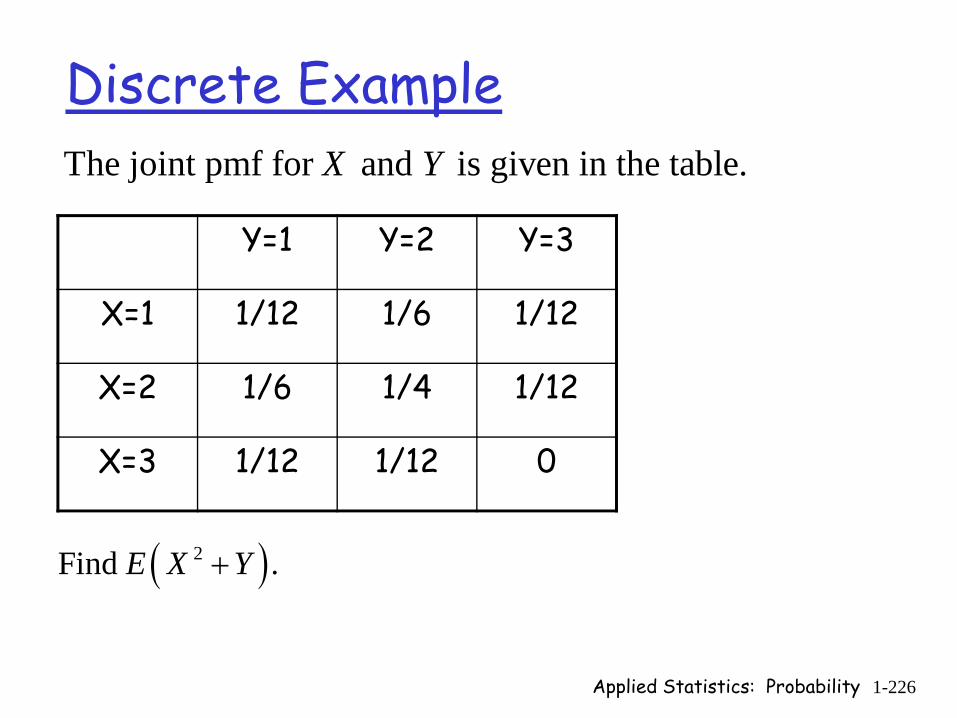
Applied Statistics: Probability 1-226
Discrete Example
Y=1 Y=2 Y=3
X=1 1/12 1/6 1/12
X=2 1/6 1/4 1/12
X=3 1/12 1/12 0
The joint pmf for and is given in the table.X Y
( )2Find .E X Y+

Applied Statistics: Probability 1-227
Continuous Example16 for ( , )
Let ( , ) where A is the triangle shown0 otherwise
x y Af x y
∈⎧= ⎨
⎩
1x = 5x =
3y =
A34 ( 1)y x= −
( ) ( )( )2Let , . What is , ?X Y X Y E X Yφ φ= +
( )( ) ( )34 ( 1)5
2 16
1 0
Solution: , 92.x
E X Y x y dydxφ−
= + =∫ ∫
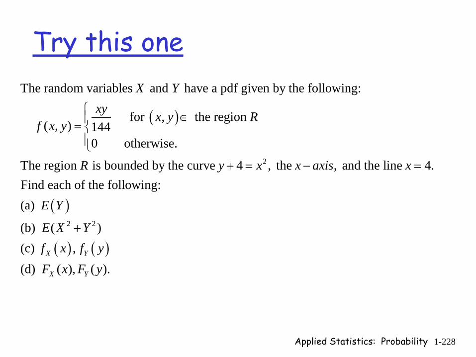
Applied Statistics: Probability 1-228
Try this one
( )
2
The random variables and have a pdf given by the following:
for , the region ( , ) 144
0 otherwise.
The region is bounded by the curve 4 , the , and the line
X Yxy x y R
f x y
R y x x axis
⎧ ∈⎪= ⎨⎪⎩
+ = −
( )
( ) ( )
2 2
4.Find each of the following:(a)
(b) ( )(c) ,(d) ( ), ( ).
X Y
X Y
x
E Y
E X Yf x f yF x F y
=
+
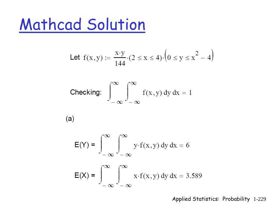
Mathcad Solution
Applied Statistics: Probability 1-229
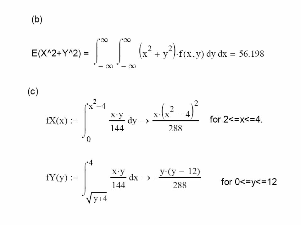
Applied Statistics: Probability 1-230
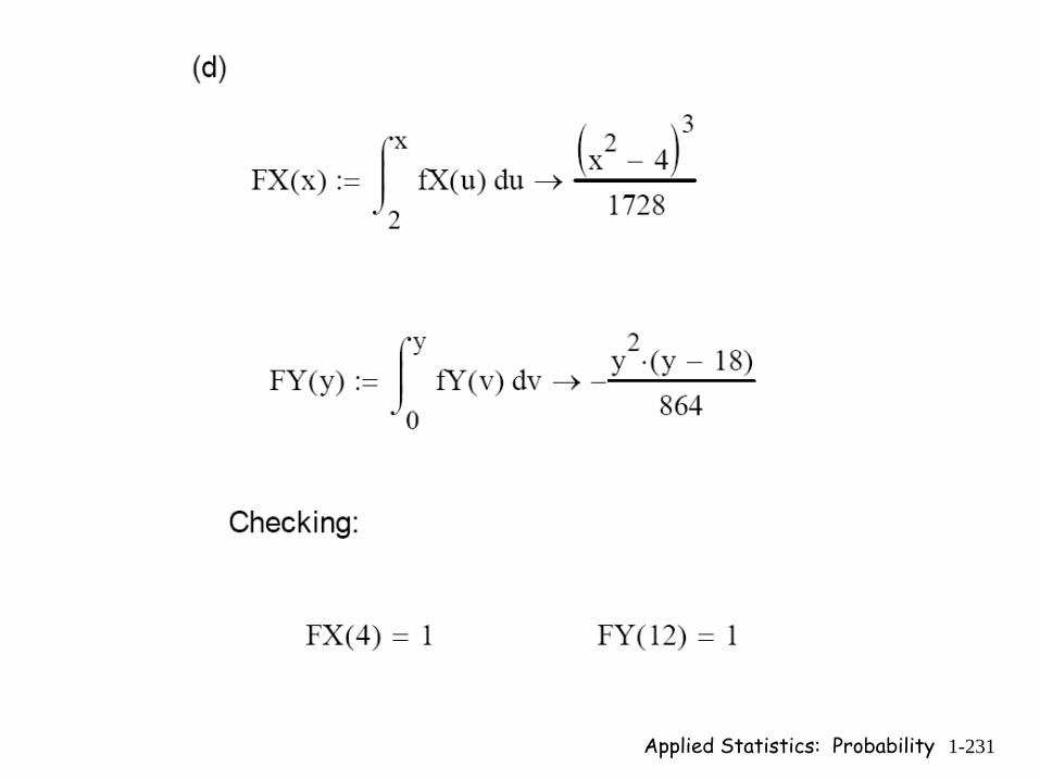
Applied Statistics: Probability 1-231
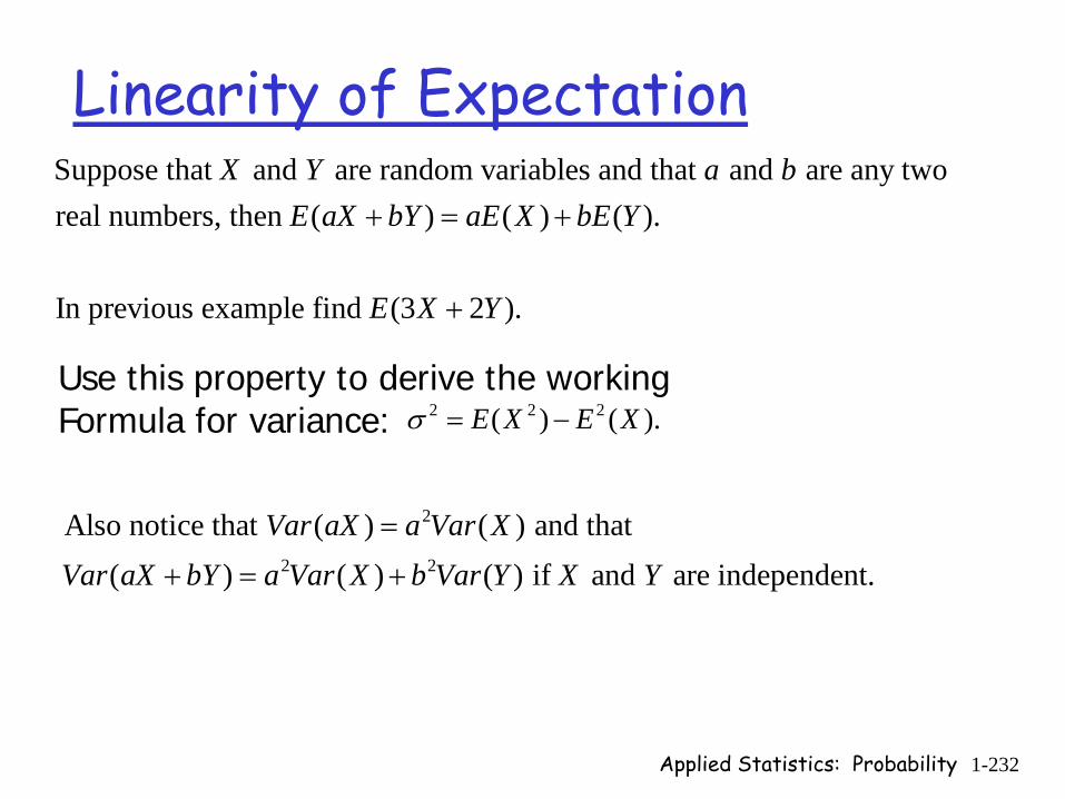
Applied Statistics: Probability 1-232
Linearity of ExpectationSuppose that and are random variables and that and are any tworeal numbers, then ( ) ( ) ( ).
In previous example find (3 2 ).
X Y a bE aX bY aE X bE Y
E X Y
+ = +
+
Use this property to derive the working Formula for variance: 2 2 2( ) ( ).E X E Xσ = −
2
2 2
Also notice that ( ) ( ) and that ( ) ( ) ( ) if and are independent.
Var aX a Var XVar aX bY a Var X b Var Y X Y
=
+ = +
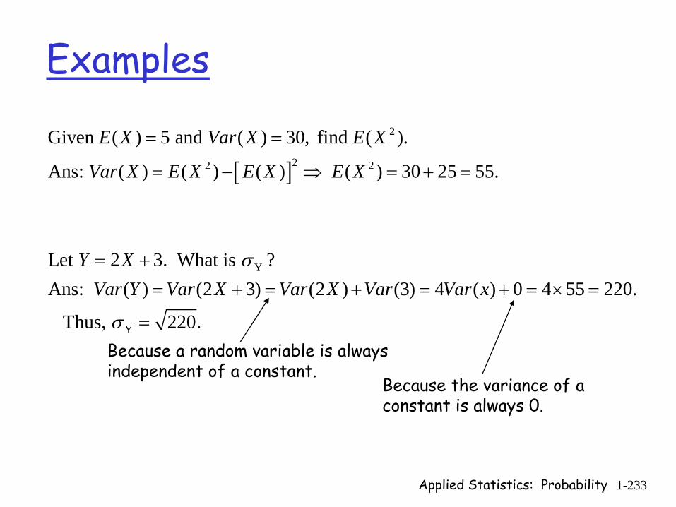
Applied Statistics: Probability 1-233
Examples
[ ]
2
22 2
Y
Y
Given ( ) 5 and ( ) 30, find ( ).
Ans: ( ) ( ) ( ) ( ) 30 25 55.
Let 2 3. What is ?Ans: ( ) (2 3) (2 ) (3) 4 ( ) 0 4 55 220.
Thus, 220.
E X Var X E X
Var X E X E X E X
Y XVar Y Var X Var X Var Var x
σ
σ
= =
= − ⇒ = + =
= += + = + = + = × =
=Because a random variable is always independent of a constant.
Because the variance of a constant is always 0.
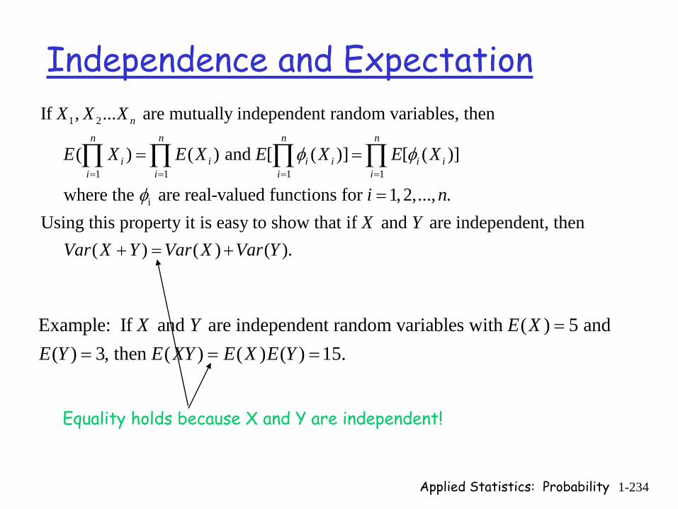
Applied Statistics: Probability 1-234
Independence and Expectation1 2
1 1 1 1
i
If , ... are mutually independent random variables, then
( ) ( ) and [ ( )] [ ( )]
where the are real-valued functions for 1, 2,..., .Using this property
n
n n n n
i i i i i ii i i i
X X X
E X E X E X E X
i n
φ φ
φ= = = =
= =
=
∏ ∏ ∏ ∏
it is easy to show that if and are independent, then ( ) ( ) ( ).
X YVar X Y Var X Var Y+ = +
Example: If and are independent random variables with ( ) 5 and ( ) 3, then ( ) ( ) ( ) 15.
X Y E XE Y E XY E X E Y
== = =
Equality holds because X and Y are independent!
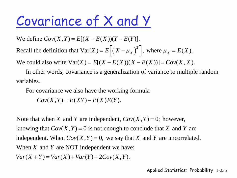
Applied Statistics: Probability 1-235
Covariance of X and Y
( )2
We define ( , ) [( ( ))( ( )].
Recall the definition that Var( ) , where ( ).
We could also write Var( ) [( ( ))( ( ))] ( , ). In other words, covariance is a generali
X X
Cov X Y E X E X Y E Y
X E X E X
X E X E X X E X Cov X X
μ μ
= − −
⎡ ⎤= − =⎣ ⎦= − − =
zation of variance to multiple randomvariables. For covariance we also have the working formula ( , ) ( ) ( ) ( ).
Note that when and are independent, ( , ) 0; however,k
Cov X Y E XY E X E Y
X Y Cov X Y
= −
=nowing that ( , ) 0 is not enough to conclude that and are
independent. When ( , ) 0, we say that and are uncorrelated.When and are NOT independent we have:
( ) ( ) ( ) 2
Cov X Y X YCov X Y X Y
X YVar X Y Var X Var Y Co
==
+ = + + ( , ).v X Y
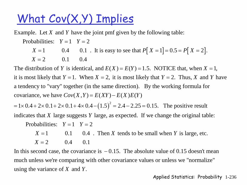
Applied Statistics: Probability 1-236
What Cov(X,Y) Implies
[ ] [ ]
Example. Let and have the joint pmf given by the following table:Probabilities: 1 2
1 0.4 0.1 . It is easy to see that 1 0.5 2 .2 0.1 0.4
The distribution of is identical, and ( ) (
X YY Y
X P X P XX
Y E X E
= == = = = ==
= ) 1.5. NOTICE that, when 1,it is most likely that 1. When 2, it is most likely that 2. Thus, and havea tendency to "vary" together (in the same direction). By the working formula for
Y XY X Y X Y
= == = =
( )2
covariance, we have ( , ) ( ) ( ) ( )
1 0.4 2 0.1 2 0.1 4 0.4 1.5 2.4 2.25 0.15. The positive resultindicates that large suggests large, as expected. If we change the original table:
Cov X Y E XY E X E Y
X Y
= −
= × + × + × + × − = − =
Probabilities: 1 2 1 0.1 0.4 . Then tends to be small when is large, etc.
2 0.4 0.1In this second case, the covariance is 0.15. The absolute value of 0.15 doesn't meanmuch unless we're compa
Y YX X YX
= ===
−ring with other covariance values or unless we "normalize"
using the variance of and .
X Y
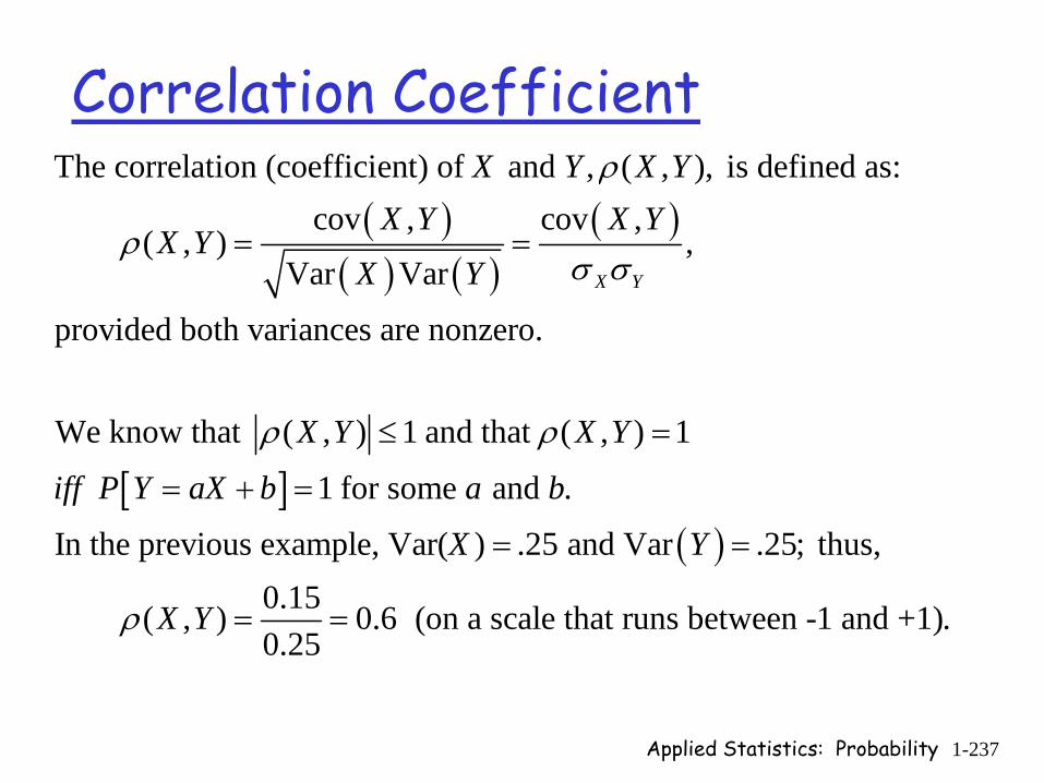
Applied Statistics: Probability 1-237
Correlation Coefficient
( )( ) ( )
( )
[ ]
The correlation (coefficient) of and , ( , ), is defined as:cov , cov ,
( , ) ,Var Var
provided both variances are nonzero.
We know that ( , ) 1 and that ( , ) 1
1 for s
X Y
X Y X YX Y X Y
X YX Y
X Y X Y
iff P Y aX b
ρ
ρσ σ
ρ ρ
= =
≤ =
= + =
( )ome and .
In the previous example, Var( ) .25 and Var .25; thus, 0.15 ( , ) 0.6 (on a scale that runs between -1 and +1).0.25
a b
X Y
X Yρ
= =
= =

Applied Statistics: Probability 1-238
Student Exercise
, , ,
, , ,
The random variables and are jointly distributed as follows:1 1 1 (1,1) (1, 2) (2, 2) 6 6 61 1 1 (2,3) (3,3) (3,4) .6 6 6
Find the covariance and correlation of
X Y X Y X Y
X Y X Y X Y
X Y
P P P
P P P
= = =
= = =
and .X Y
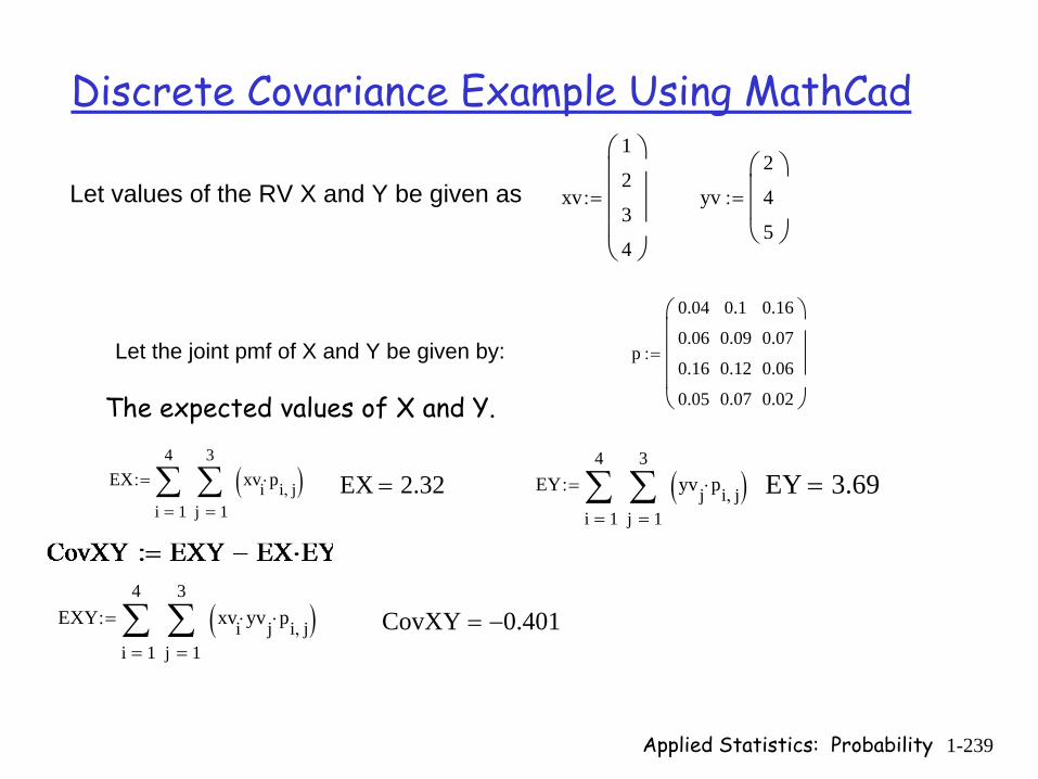
Applied Statistics: Probability 1-239
Discrete Covariance Example Using MathCad
The expected values of X and Y.
Let values of the RV X and Y be given as xv
1
2
3
4
⎛⎜⎜⎜⎜⎝
⎞⎟⎟⎟⎟⎠
:= yv
2
4
5
⎛⎜⎜⎝
⎞⎟⎟⎠
:=
Let the joint pmf of X and Y be given by: p
0.04
0.06
0.16
0.05
0.1
0.09
0.12
0.07
0.16
0.07
0.06
0.02
⎛⎜⎜⎜⎜⎝
⎞⎟⎟⎟⎟⎠
:=
EX
1
4
i 1
3
j
xvi pi j, ⋅( )∑=
∑=
:= EX 2.32= EY
1
4
i 1
3
j
yvj pi j, ⋅( )∑=
∑=
:= EY 3.69=
EXY
1
4
i 1
3
j
xvi yvj⋅ pi j, ⋅( )∑=
∑=
:= CovXY 0.401−=
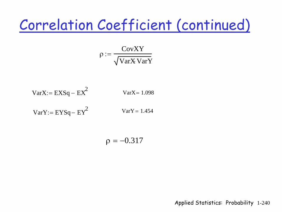
Applied Statistics: Probability 1-240
Correlation Coefficient (continued)
ρCovXY
VarX VarY⋅:=
VarX EXSq EX2−:=
VarY EYSq EY2−:=
VarX 1.098=
VarY 1.454=
ρ 0.317−=