Embed Size (px)
Citation preview
Probability Models and StatisticalMethods in Reliability
Larry LeemisDepartment of Mathematics
College of William and MaryWilliamsburg, VA 23187-8795
[email protected] 757-221-2034
Undergraduate Simulation, Modeling and AnalysisFebruary 14, 2000
Outline1. Introduction2. Coherent Systems Analysis3. Lifetime Distributions4. Parametric Lifetime Models5. Specialized Models6. Repairable Systems7. Lifetime Data Analysis8. Fitting Parametric Models to Data9. Parametric Estimation for Models with Covariates10. Nonparametric Methods11. Assessing Model Adequacy

1. Introduction
Motivation• Space Shuttle Challenger accident• Chernobyl and Three Mile Island accidents• product liability• customer goodwill• corporate reputation
Three closely-related fields of study• Actuarial science• Biostatistics• Reliability engineering
TerminologyThe event at the end of a lifetime is called
• a failure by reliability engineers• death by actuaries and biostatisticians• an epoch by point process researchers
The object of a study is called• a system, component or item by reliability
engineers• an individual by actuaries• an organism by biostatisticians
To avoid switching terms, failure of an item will beused here.
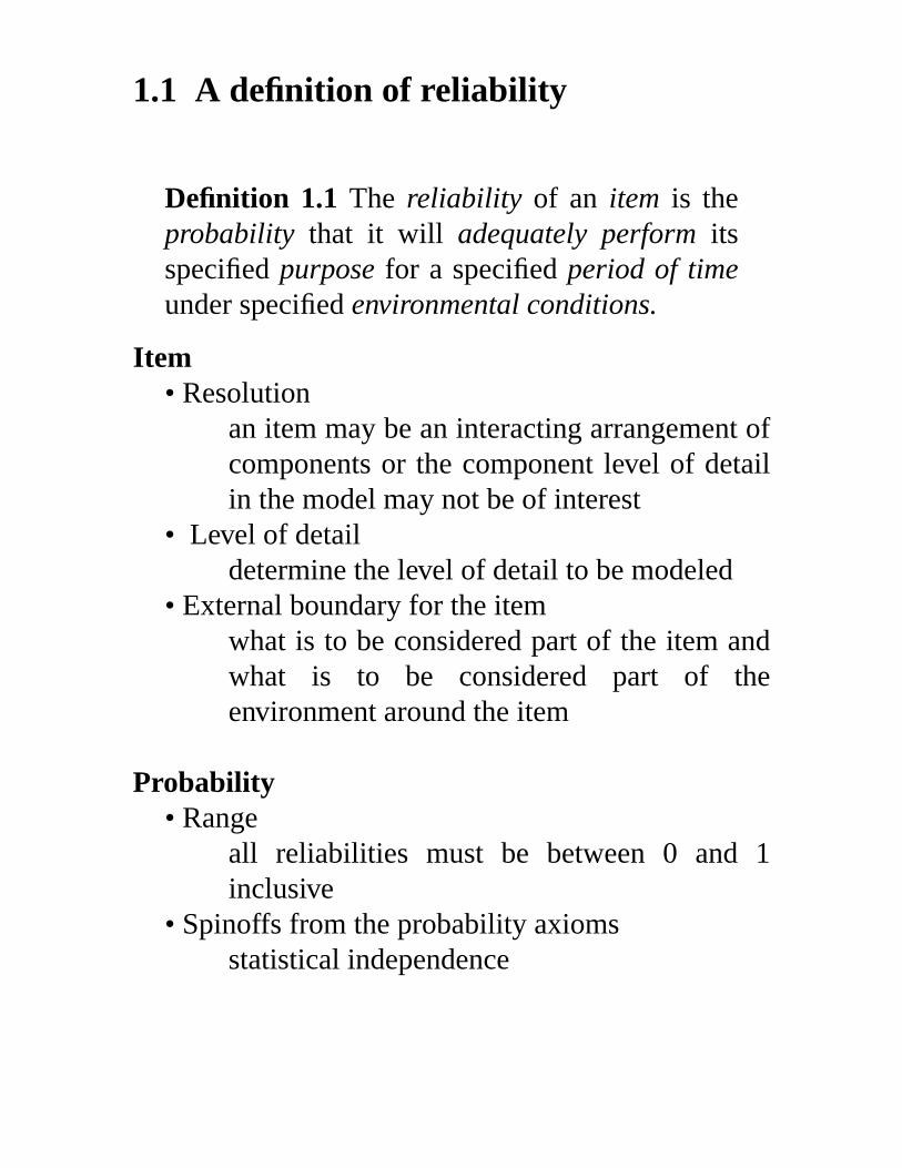
1.1 A definition of reliability
Definition 1.1 The reliability of an item is theprobability that it will adequately perform itsspecified purpose for a specified period of timeunder specified environmental conditions.
Item• Resolution
an item may be an interacting arrangement ofcomponents or the component level of detailin the model may not be of interest
• Lev el of detaildetermine the level of detail to be modeled
• External boundary for the itemwhat is to be considered part of the item andwhat is to be considered part of theenvironment around the item
Probability• Range
all reliabilities must be between 0 and 1inclusive
• Spinoffs from the probability axiomsstatistical independence
Adequate performance• Must be stated unambiguously• Standards
Example: a ball bearing has failed when itsdiameter falls outside of 3 + 0.05 mm
• Binary modelsthe item is in either the functioning or failedstate (e.g., a fuse)
Purpose• Intended use
Example: a drill may have one grade for ahandyman and another for a contractor
Time• Units
must be specified (e.g., hours, years)• Notation
many lifetime models use the randomvariable T
• Time need not be taken literallyconsider an automobile tire, light switch
• Time duration must be specifiedExample: 1000 hour reliability is 0.8
• Continuous operation vs. on/off cyclingtime alone may not be the only consideration(e.g., motors, computers)
Environmental conditions• Factors
temperature, humidity, and turning speed allaffect the lifetime of a machine tool
• Preventive maintenanceusually effective in prolonging the lifetime ofthe item and hence increasing the reliability
Reliability vs. quality• reliability incorporates the passage of time• quality is a static descriptor of an item
Example 1: Tw o transistors of equal quality. Oneused in a television set, the other in a cannonlaunch environment. Identical quality, differentreliabilities.
Example 2: Tw o automobile tires, each of highquality. One was produced in 1957, the other in1994. Same purpose, different reliabilities dueto improved design (e.g., tread or steel belts),components (e.g., rubber) or processes (e.g.,manufacturing advances). Some qualityimprovements (e.g., improved tread design)improve the reliability of the tire, while others(e.g., improved white wall design) will not.

1.2 Case study
Item under consideration: the O-rings on the solidrocket motors on the Space Shuttle
Subsystems• orbiter• external liquid-fuel tank• two solid rocket motors
Each assembled solid rocket motor contains threefield joints that must be sealed.
O-rings• 37.5 feet in diameter• 0.28 inches thick• all six O-rings must operate to avoid having the
propellant escape causing potential failure, sothe O-rings form a six-component series system
Figure 1.1 A six-component seriesarrangement of O-rings.

Redundancy: a technique to increase reliability• Redundancy is highly effective if the components
are independent.• In 1977, NASA discovered field joint rotation
indicating that the failure of the primary andsecondary O-rings may not be independent.
• Prior to the Challenger accident, the solid rocketmotors were recovered in 23 of the 24 shuttleflights.
• There was concern that an environmentalvariable, temperature at launch, might influencethe reliability of the field joints.
• There was a forecast of 31oF for the morning ofthe launch of the Challenger, the coldest launchtemperature to date.
Figure 1.2 A 12-componentarrangement of O-rings.
•
•• •
• •••• •
•
•
•
• •• •
•
•• •• •
Temperature
55 60 65 70 75 80 85
0.0
0.5
1.0
1.5
2.0
2.5
3.0Failures
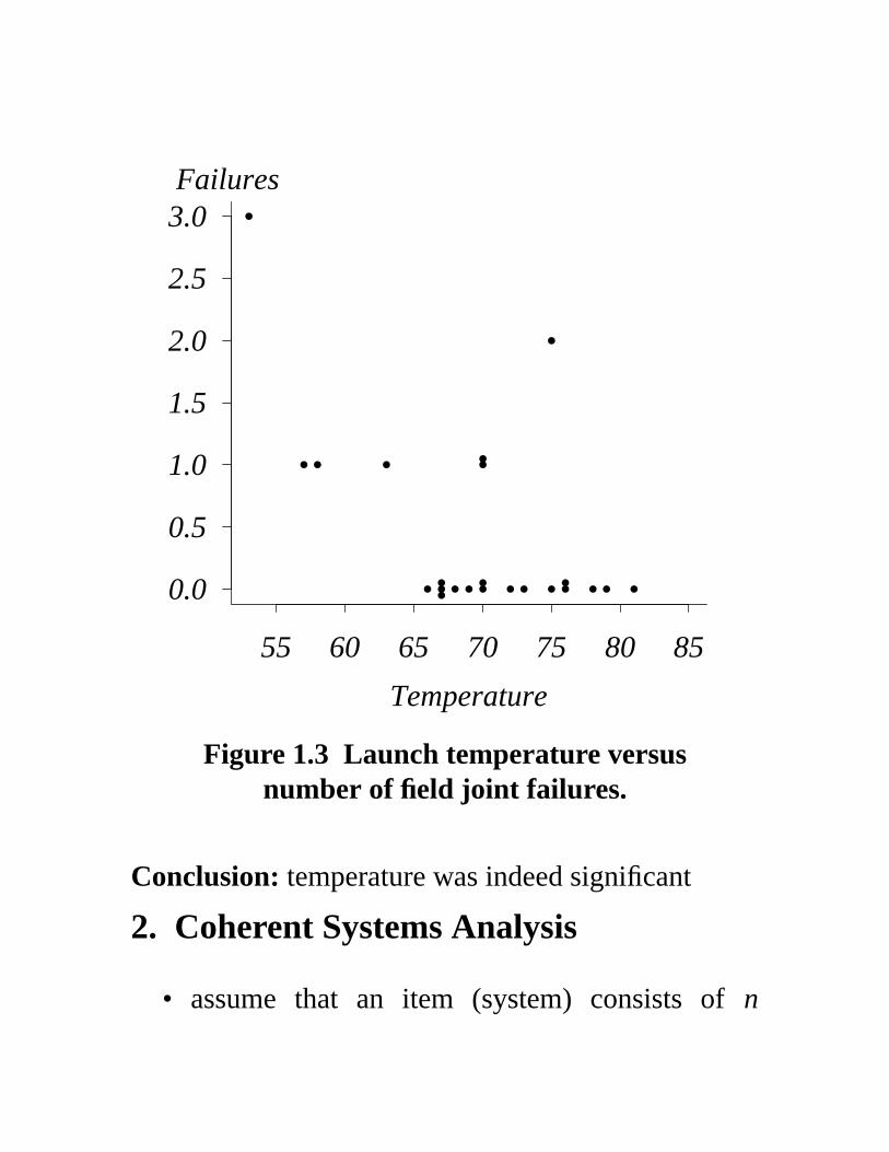
Figure 1.3 Launch temperature versusnumber of field joint failures.
Conclusion: temperature was indeed significant
2. Coherent Systems Analysis
• assume that an item (system) consists of n
components• two key modeling decisions
which elements of the system are includedthe level of detail
• the first two sections: structural properties• the next two sections: probabilistic properties• outline
structure functionsminimal path and cut setsreliability functionsreliability bounds
2.1 Structure functions
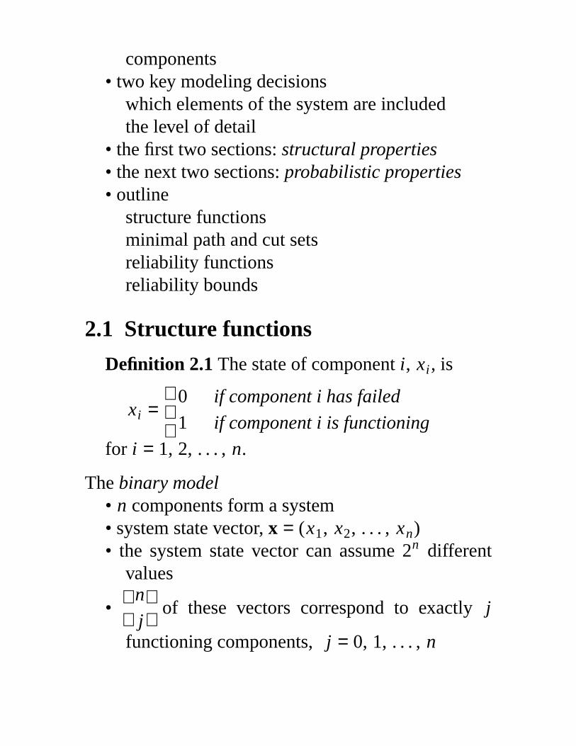
Definition 2.1 The state of component i, xi , is
xi =
0
1
if component i has failed
if component i is functioning
for i = 1, 2, . . . , n.
The binary model• n components form a system• system state vector, x = (x1, x2, . . . , xn)• the system state vector can assume 2n different
values
•
n
j
of these vectors correspond to exactly j
functioning components, j = 0, 1, . . . , n
• the structure function, φ (x), maps the systemstate vector x to 0 or 1, the system state
Definition 2.2 The structure function φ is
φ (x) =
0
1
if the system has failed under xif the system is functioning under x.
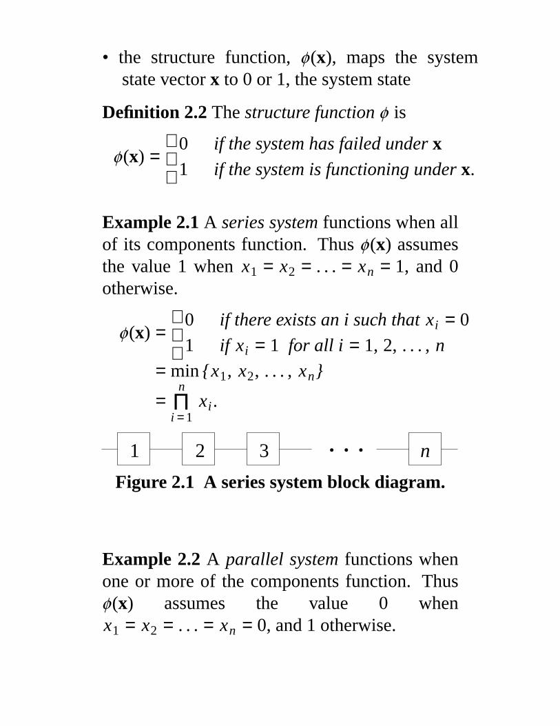
Example 2.1 A series system functions when allof its components function. Thus φ (x) assumesthe value 1 when x1 = x2 = . . . = xn = 1, and 0otherwise.
φ (x) =
0
1
if there exists an i such that xi = 0
if xi = 1 for all i = 1, 2, . . . , n
= min {x1, x2, . . . , xn}
=n
i = 1Π xi .
1 2 n. . . 3
Figure 2.1 A series system block diagram.
Example 2.2 A parallel system functions whenone or more of the components function. Thusφ (x) assumes the value 0 whenx1 = x2 = . . . = xn = 0, and 1 otherwise.
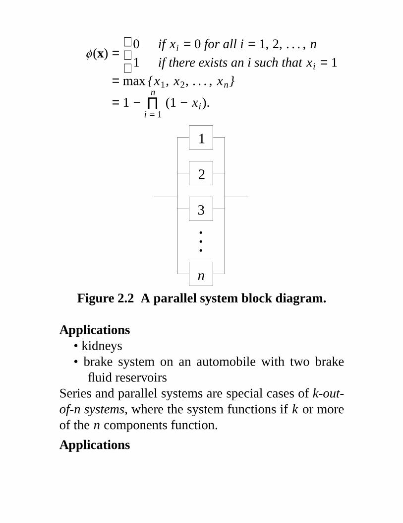
φ (x) =
0
1
if xi = 0 for all i = 1, 2, . . . , n
if there exists an i such that xi = 1= max {x1, x2, . . . , xn}
= 1 −n
i = 1Π (1 − xi).
2
...
3
1
n
Figure 2.2 A parallel system block diagram.
Applications• kidneys• brake system on an automobile with two brake
fluid reservoirsSeries and parallel systems are special cases of k-out-of-n systems, where the system functions if k or moreof the n components function.
Applications
• suspension bridge (components: cables)• an automobile engine (components: cylinders)• a bicycle wheel (components: spokes)
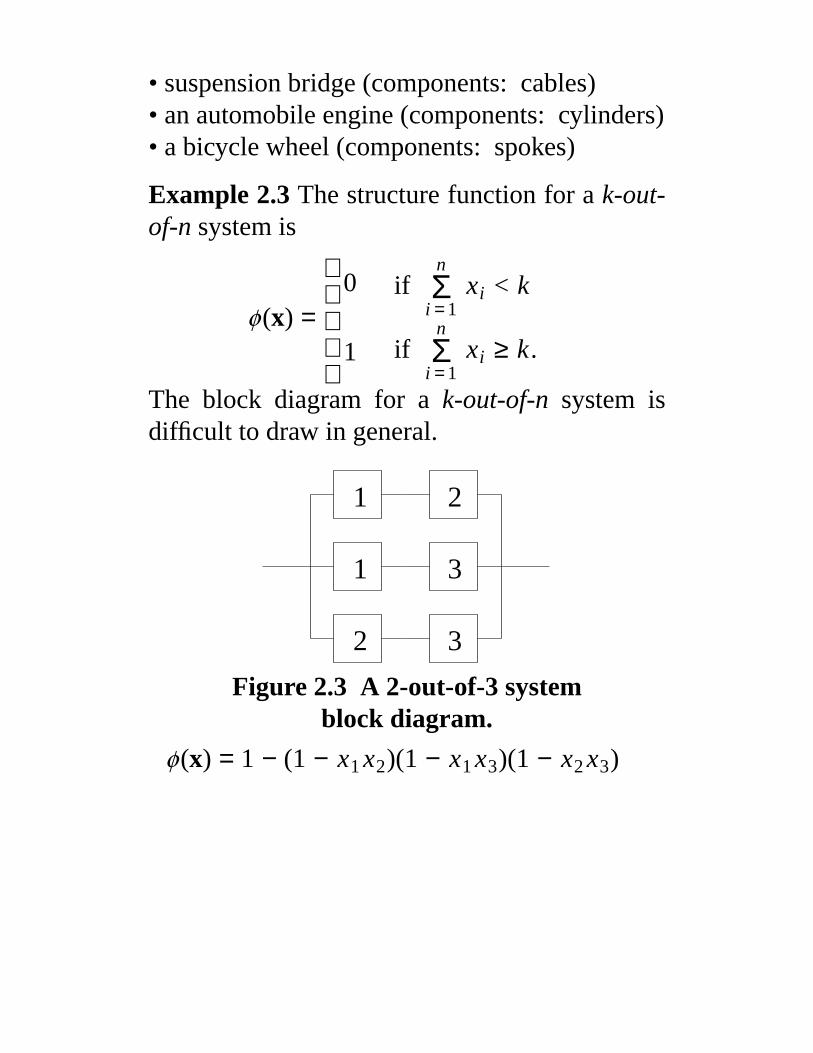
Example 2.3 The structure function for a k-out-of-n system is
φ (x) =
0
1
ifn
i = 1Σ xi < k
ifn
i = 1Σ xi ≥ k.
The block diagram for a k-out-of-n system isdifficult to draw in general.
1
2
1
2
3
3
Figure 2.3 A 2-out-of-3 systemblock diagram.
φ (x) = 1 − (1 − x1 x2)(1 − x1 x3)(1 − x2 x3)
2.3 Reliability functions
Assumptions• the binary model applies to components and
systems• the n components must be nonrepairable• the components are independent
Definition 2.9 The random variable denotingthe state of component i, Xi , is
Xi =
0
1
if component i has failed
if component i is functioning
for i = 1, 2, . . . , n.
Random component states• these n values can be written as a random system
state vector X• pi = P[Xi = 1] is the reliability of the ith
component, i = 1, 2, . . . , n• reliability vector p = (p1, p2, . . . , pn)• must specify the time to which the reliability
applies (e.g., 5000-hour reliability is 0.83)• the system reliability, r, is defined by
r(p) = P[φ (X) = 1]• r(p) used when all component reliabilities are
equal
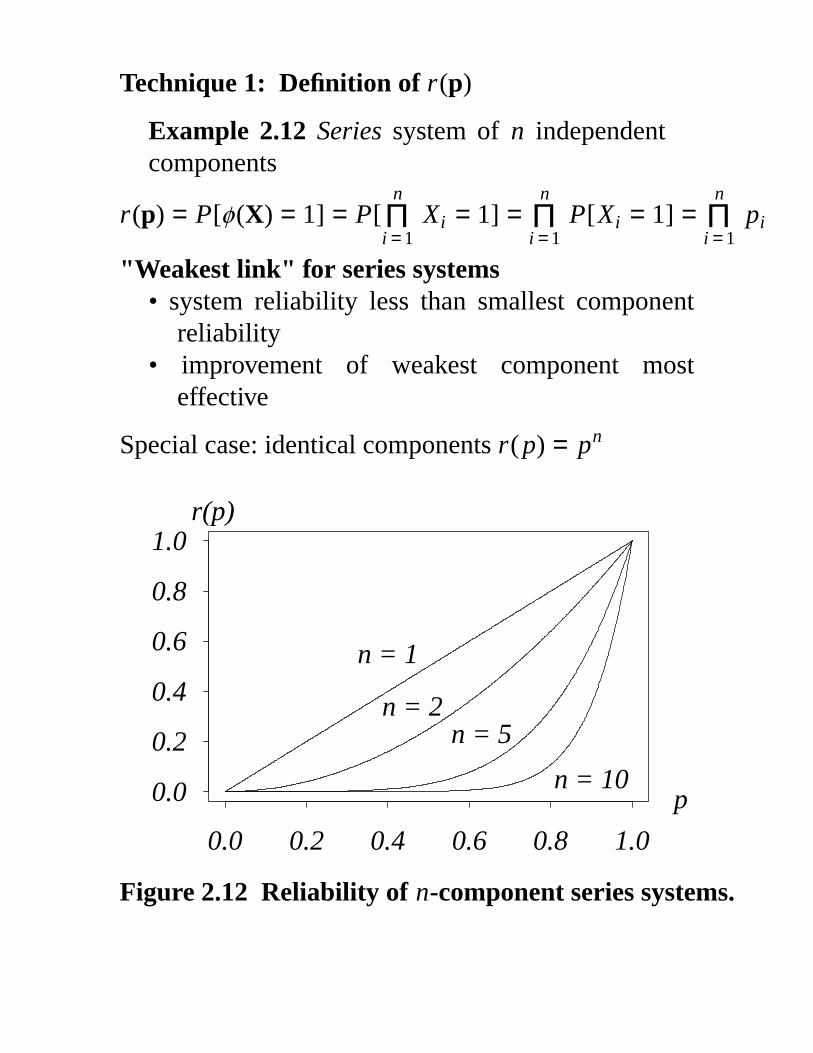
Technique 1: Definition of r(p)
Example 2.12 Series system of n independentcomponents
r(p) = P[φ (X) = 1] = P[n
i = 1Π Xi = 1] =
n
i = 1Π P[Xi = 1] =
n
i = 1Π pi
"Weakest link" for series systems• system reliability less than smallest component
reliability• improvement of weakest component most
effective
Special case: identical components r(p) = pn
0.0 0.2 0.4 0.6 0.8 1.0
0.0
0.2
0.4
0.6
0.8
1.0
n = 1
n = 2n = 5
n = 10p
r(p)
Figure 2.12 Reliability of n-component series systems.
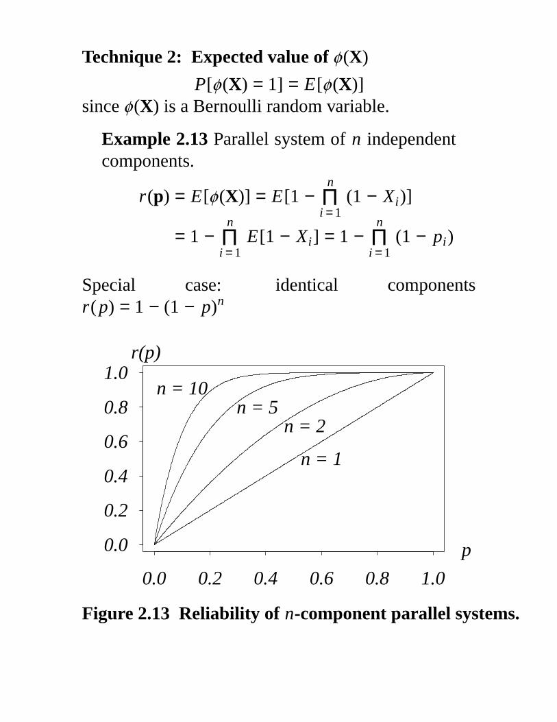
Technique 2: Expected value of φ (X)
P[φ (X) = 1] = E[φ (X)]since φ (X) is a Bernoulli random variable.
Example 2.13 Parallel system of n independentcomponents.
r(p) = E[φ (X)] = E[1 −n
i = 1Π (1 − Xi)]
= 1 −n
i = 1Π E[1 − Xi] = 1 −
n
i = 1Π (1 − pi)
Special case: identical componentsr(p) = 1 − (1 − p)n
0.0 0.2 0.4 0.6 0.8 1.0
0.0
0.2
0.4
0.6
0.8
1.0
n = 1
n = 2n = 5
n = 10
p
r(p)
Figure 2.13 Reliability of n-component parallel systems.
"Law of diminishing returns" for parallel systems• marginal gain in reliability decreases
dramatically as more components are added• improvement of the strongest component is the
most effective
Notes on parallel systems• standby system• shared-parallel system
3. Lifetime Distributions
MotivationUp to this point, reliability has only been consideredat one particular instance of time.
Outline• lifetime distribution representations• discrete distributions• moments and fractiles• system lifetime distributions• distribution classes
3.1 Distribution representations
Five functions that define the distribution of T• survivor function• probability density function• hazard function
• cumulative hazard function• mean residual lifetime function
Survivor function (reliability function)
S(t) = P[T ≥ t] t ≥ 0All survivor functions satisfy three conditions
S(0) = 1t → ∞lim S(t) = 0 S(t) is nonincreasing
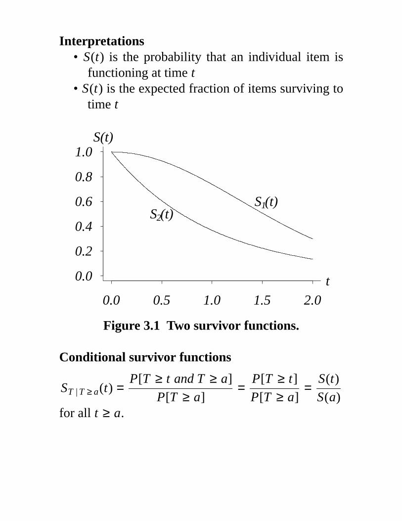
Interpretations• S(t) is the probability that an individual item is
functioning at time t• S(t) is the expected fraction of items surviving to
time t
0.0 0.5 1.0 1.5 2.0
0.0
0.2
0.4
0.6
0.8
1.0
S (t)1S (t)2
t
S(t)
Figure 3.1 Two survivor functions.
Conditional survivor functions
ST | T ≥ a(t) =P[T ≥ t and T ≥ a]
P[T ≥ a]=
P[T ≥ t]
P[T ≥ a]=
S(t)
S(a)for all t ≥ a.
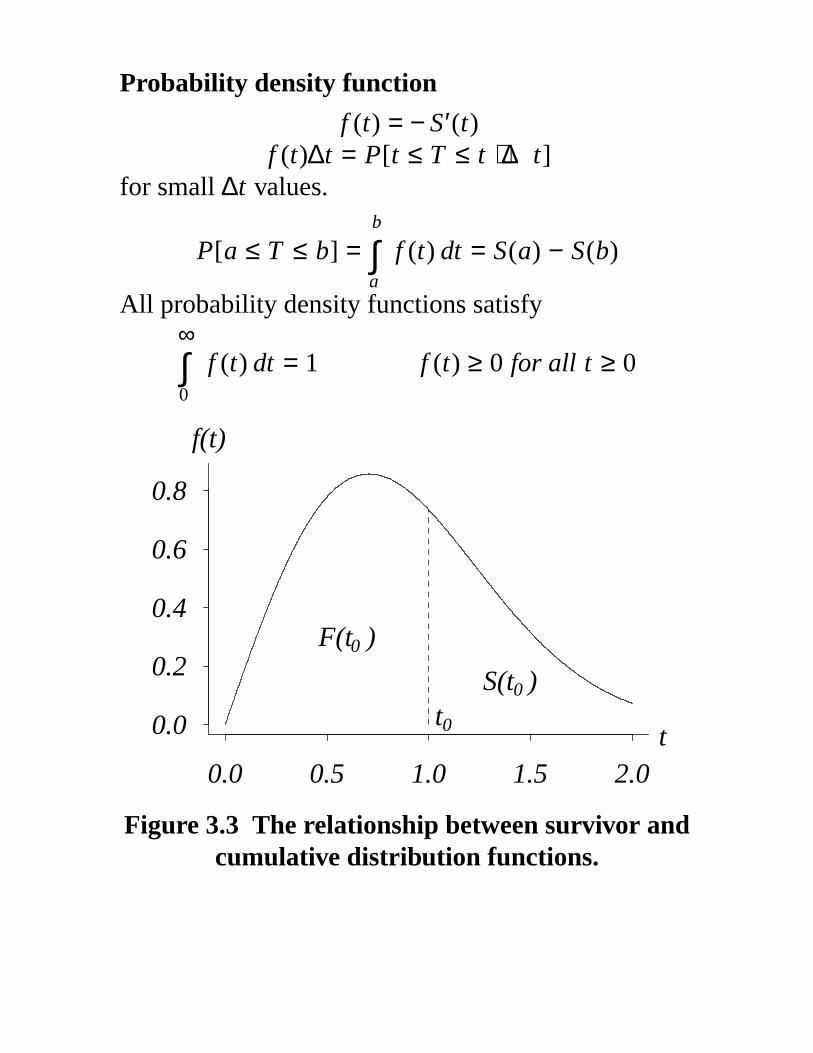
Probability density function
f (t) = − S′(t)f (t)∆t = P[t ≤ T ≤ t + ∆t]
for small ∆t values.
P[a ≤ T ≤ b] =b
a∫ f (t) dt = S(a) − S(b)
All probability density functions satisfy∞
0∫ f (t) dt = 1 f (t) ≥ 0 for all t ≥ 0
0.0 0.5 1.0 1.5 2.0
0.0
0.2
0.4
0.6
0.8
F(t )0
S(t )0
t0 t
f(t)
Figure 3.3 The relationship between survivor andcumulative distribution functions.
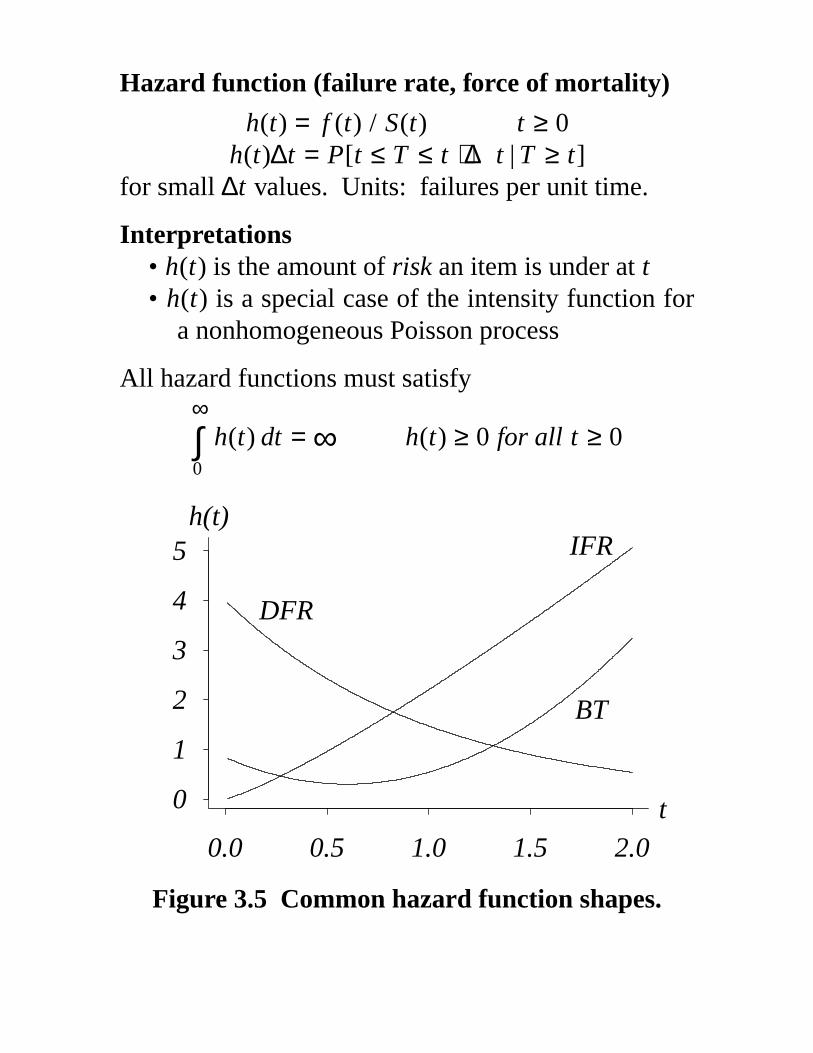
Hazard function (failure rate, force of mortality)
h(t) = f (t) / S(t) t ≥ 0h(t)∆t = P[t ≤ T ≤ t + ∆t | T ≥ t]
for small ∆t values. Units: failures per unit time.
Interpretations• h(t) is the amount of risk an item is under at t• h(t) is a special case of the intensity function for
a nonhomogeneous Poisson process
All hazard functions must satisfy∞
0∫ h(t) dt = ∞ h(t) ≥ 0 for all t ≥ 0
0.0 0.5 1.0 1.5 2.0
0
1
2
3
4
5 IFR
DFR
BT
t
h(t)
Figure 3.5 Common hazard function shapes.
Cumulative hazard function (integratedhazard function and the renewal function)
H(t) =t
0∫ h(τ )dτ t ≥ 0
All cumulative hazard functions satisfy
H(0) = 0t → ∞lim H(t) = ∞ H(t) is nondecreasing
Applications• variate generation in Monte Carlo simulation• implementing certain procedures in statistical
inference• defining certain distribution classes
Mean residual life function
L(t) = E[T − t | T ≥ t] =1
S(t)
∞
t∫ τ f (τ )dτ − t t ≥ 0
All mean residual life functions satisfy
L(t) ≥ 0 L′(t) ≥ − 1∞
0∫
dt
L(t)= ∞
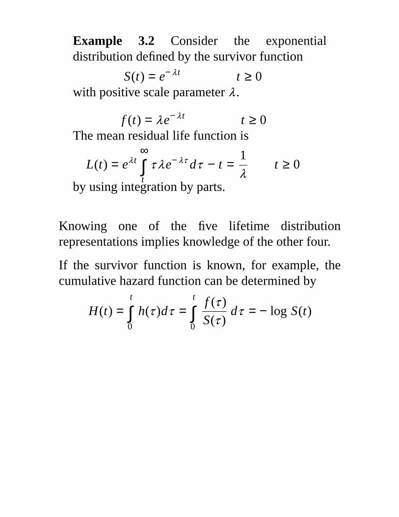
Example 3.2 Consider the exponentialdistribution defined by the survivor function
S(t) = e− λ t t ≥ 0with positive scale parameter λ .
f (t) = λe− λ t t ≥ 0The mean residual life function is
L(t) = eλ t∞
t∫ τ λe− λτ dτ − t =
1
λt ≥ 0
by using integration by parts.
Knowing one of the five lifetime distributionrepresentations implies knowledge of the other four.
If the survivor function is known, for example, thecumulative hazard function can be determined by
H(t) =t
0∫ h(τ )dτ =
t
0∫
f (τ )
S(τ )dτ = − log S(t)
3.3 Moments and fractiles
MotivationMoments and fractiles contain less information than alifetime distribution representation, but they are oftenuseful ways to summarize the distribution of arandom lifetime.
Examples• the mean time to failure, E(T )• the median, t0.50
• the 95th percentile of a distribution, t0.95
Assumption: random lifetime T is continuous
E[u(T )] =∞
0∫ u(t) f (t) dt
Mean (abbreviated by MTTF or MTBF)
µ = E[T ] =∞
0∫ t f (t) dt =
∞
0∫ S(t) dt
Variance
σ 2 = V [T ] = E[(T − µ)2] = E[T 2] − (E[T ])2
Coefficient of variation
γ =σµ
Skewness
γ3 = E
T − µσ
3
Kurtosis
γ4 = E
T − µσ
4
Fractiles: t p satisfies
F(t p) = P[T ≤ t p] = p or t p = F −1( p )
Example 3.5 The exponential distribution hassurvivor function
S(t) = e− λ t t ≥ 0
µ = E[T ] =∞
0∫ S(t) dt =
∞
0∫ e− λ t dt =
1
λ
E[T 2] =∞
0∫ t2 f (t) dt =
∞
0∫ t2 λ e− λ t dt =
2
λ2
σ 2 = E[T 2] − (E[T ])2 =2
λ2−
1
λ2=
1
λ2
γ3 = λ36λ− 3 − 6λ− 3 + 3λ− 3 − λ− 3
= 2
t p = −1
λlog (1 − p)
4. Parametric Lifetime Models
MotivationSurvival patterns of a drill bit, a fuse, and anautomobile are vastly different.
Outline• parameters• exponential• Weibull• gamma• other distributions
4.1 Parameters
Three types of parameters:• location• scale• shape
Location (or shift) parametersShift a distribution along the time axis. If c1
and c2 are two values of a location parameterfor a lifetime distribution with survivor functionS(t; c), then there exists a constant α such thatS(t; c1) = S(α + t; c2).
Example Mean µ in the normaldistribution.
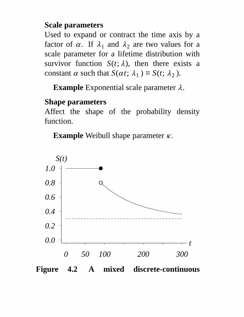
Scale parametersUsed to expand or contract the time axis by afactor of α . If λ1 and λ2 are two values for ascale parameter for a lifetime distribution withsurvivor function S(t; λ), then there exists aconstant α such that S(α t; λ1 ) = S(t; λ2 ).
Example Exponential scale parameter λ .
Shape parametersAffect the shape of the probability densityfunction.
Example Weibull shape parameter κ .
0 50 100 200 300
0.0
0.2
0.4
0.6
0.8
1.0 O
O
OOOOOOOOOOOOOOOOOOO
t
S(t)
Figure 4.2 A mixed discrete-continuous

survivor function.
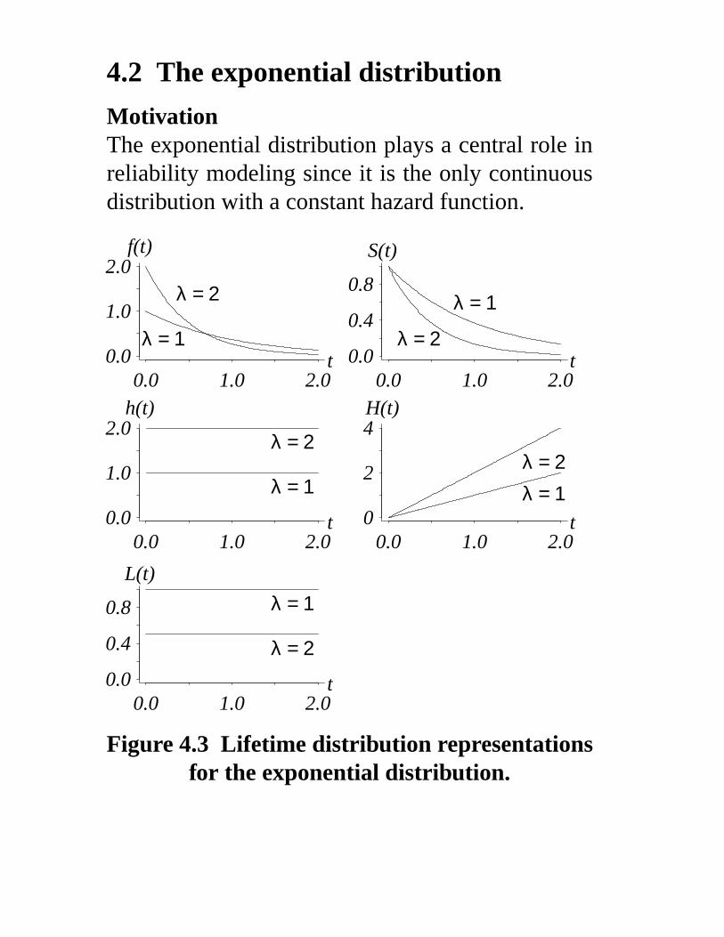
4.2 The exponential distribution
MotivationThe exponential distribution plays a central role inreliability modeling since it is the only continuousdistribution with a constant hazard function.
0.0 1.0 2.00.0
1.0
2.0
λ = 1
λ = 2
t
f(t)
0.0 1.0 2.00.0
0.4
0.8λ = 1
λ = 2t
S(t)
0.0 1.0 2.00.0
1.0
2.0
λ = 1
λ = 2
t
h(t)
0.0 1.0 2.00
2
4
λ = 1λ = 2
t
H(t)
0.0 1.0 2.00.0
0.4
0.8 λ = 1
λ = 2
t
L(t)
Figure 4.3 Lifetime distribution representationsfor the exponential distribution.
S(t) = e− λ t f (t) = λe− λ t h(t) = λ
H(t) = λ t L(t) =1
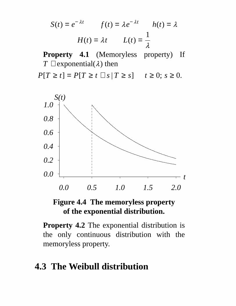
λProperty 4.1 (Memoryless property) IfT ∼ exponential(λ) then
P[T ≥ t] = P[T ≥ t + s | T ≥ s] t ≥ 0; s ≥ 0.
0.0 0.5 1.0 1.5 2.0
0.0
0.2
0.4
0.6
0.8
1.0
t
S(t)
Figure 4.4 The memoryless propertyof the exponential distribution.
Property 4.2 The exponential distribution isthe only continuous distribution with thememoryless property.
4.3 The Weibull distribution
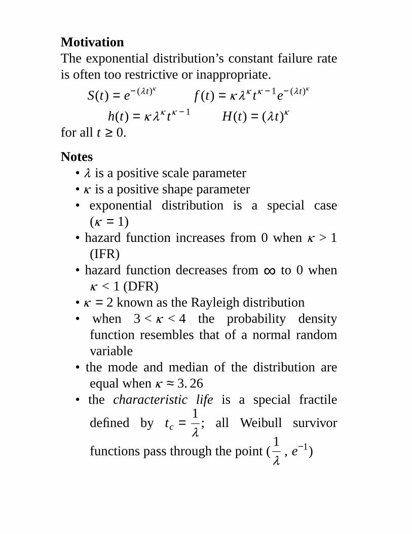
MotivationThe exponential distribution’s constant failure rateis often too restrictive or inappropriate.
S(t) = e− (λ t)κf (t) = κ λκ tκ − 1e− (λ t)κ
h(t) = κ λκ tκ − 1 H(t) = (λ t)κ
for all t ≥ 0.
Notes• λ is a positive scale parameter• κ is a positive shape parameter• exponential distribution is a special case
(κ = 1)• hazard function increases from 0 when κ > 1
(IFR)• hazard function decreases from ∞ to 0 when
κ < 1 (DFR)• κ = 2 known as the Rayleigh distribution• when 3 < κ < 4 the probability density
function resembles that of a normal randomvariable
• the mode and median of the distribution areequal when κ ≈ 3. 26
• the characteristic life is a special fractile
defined by tc =1
λ; all Weibull survivor
functions pass through the point (1
λ, e−1)
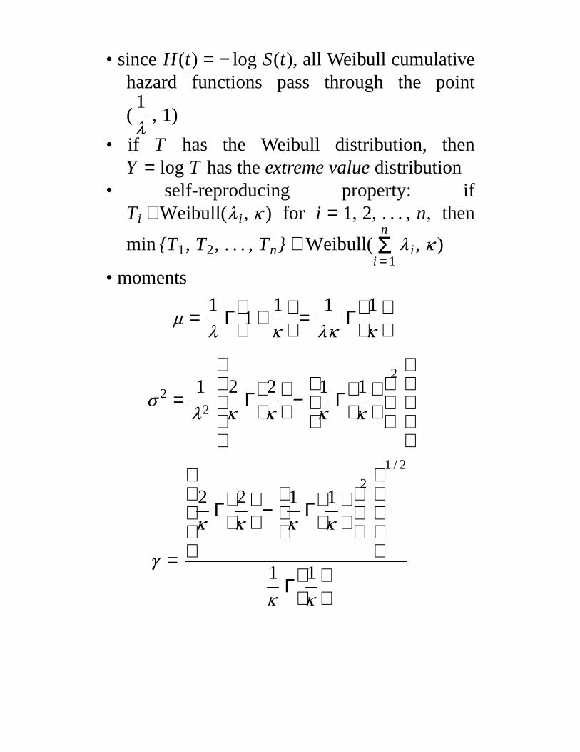
• since H(t) = − log S(t), all Weibull cumulativehazard functions pass through the point
(1
λ, 1)
• if T has the Weibull distribution, thenY = log T has the extreme value distribution
• self-reproducing property: ifTi ∼ Weibull(λ i , κ ) for i = 1, 2, . . . , n, then
min {T1, T2, . . . , Tn} ∼ Weibull(n
i = 1Σ λ i , κ )
• moments
µ =1
λΓ
1 +
1
κ
=1
λκΓ
1
κ
σ 2 =1
λ2
2
κΓ
2
κ
−
1
κΓ
1
κ
2
γ =
2
κΓ
2
κ
−
1
κΓ
1
κ
2
1 / 2
1
κΓ
1
κ
0.0 1.00.0
0.4
0.8
1.2κ = 0.5
κ = 1
κ = 2κ = 3
t
f(t)
0.0 1.00.00.20.40.60.81.0
κ = 0.5κ = 1κ = 2κ = 3
t
S(t)
0.0 1.00
2
4
6
κ = 0.5
κ = 1
κ = 2
κ = 3
t
h(t)
0.0 1.00
1
2
3
κ = 0.5κ = 1
κ = 2
κ = 3
t
H(t)
0.0 1.00
1
2
3
4κ = 0.5
κ = 1κ = 2κ = 3
t
L(t)
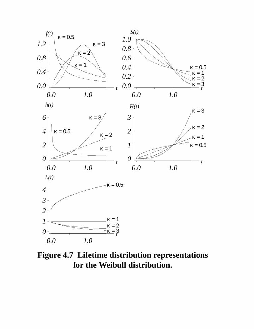
Figure 4.7 Lifetime distribution representationsfor the Weibull distribution.

4.5 Other lifetime distributions
Table 4.4 Distribution classes.
Distribution IFR DFR BT UBT
Exponential YES YES NO NO
Muth YES NO NO NO
Weibull YES YES NO NO
Gamma YES YES NO NO
Uniform YES NO NO NO
Log normal NO NO NO YES
Log logistic NO YES NO YES
Inv. Gaussian NO NO NO YES
Expon. power YES NO YES NO
Pareto NO YES NO NO
Gompertz YES NO NO NO
Makeham YES NO NO NO
IDB YES YES YES NO
Gen. Pareto YES YES NO NO
5. Specialized Models
MotivationThere are several ways to combine and extend thecontinuous lifetime models previously outlined.
Outline• competing risks• mixtures• accelerated life• proportional hazards
5.1 Competing risks
Notes• causes of failure may be grouped into k
classes• an item is subject to k competing risks (or
causes) C1, C2, . . . , Ck
• can be thought of as a series system ofcomponents
• origins of competing risks theory traced to astudy by Daniel Bernoulli in the 1700’sconcerning the impact of eliminatingsmallpox
• a second and equally appealing use ofcompeting risks models is that they can beused to combine component distributions to
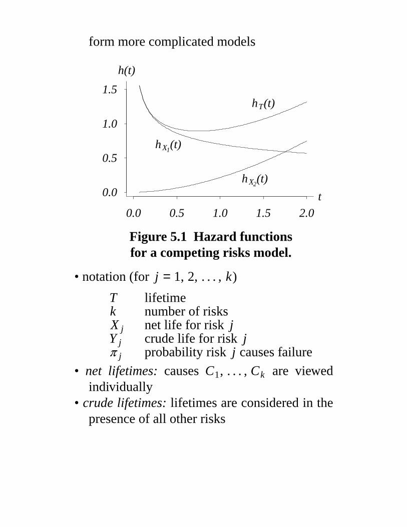
form more complicated models
0.0 0.5 1.0 1.5 2.0
0.0
0.5
1.0
1.5
h (t)X2
h (t)X1
h (t)T
t
h(t)
Figure 5.1 Hazard functionsfor a competing risks model.
• notation (for j = 1, 2, . . . , k)
T lifetimek number of risksX j net life for risk jY j crude life for risk jπ j probability risk j causes failure
• net lifetimes: causes C1, . . . , Ck are viewedindividually
• crude lifetimes: lifetimes are considered in thepresence of all other risks
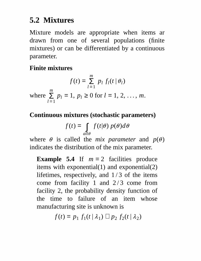
5.2 Mixtures
Mixture models are appropriate when items ardrawn from one of several populations (finitemixtures) or can be differentiated by a continuousparameter.
Finite mixtures
f (t) =m
l = 1Σ pl fl(t |θ l)
wherem
l = 1Σ pl = 1, pl ≥ 0 for l = 1, 2, . . . , m.
Continuous mixtures (stochastic parameters)
f (t) =allθ∫ f (t |θ ) p(θ )dθ
where θ is called the mix parameter and p(θ )indicates the distribution of the mix parameter.
Example 5.4 If m = 2 facilities produceitems with exponential(1) and exponential(2)lifetimes, respectively, and 1 / 3 of the itemscome from facility 1 and 2 / 3 come fromfacility 2, the probability density function ofthe time to failure of an item whosemanufacturing site is unknown is
f (t) = p1 f1(t | λ1) + p2 f2(t | λ2)
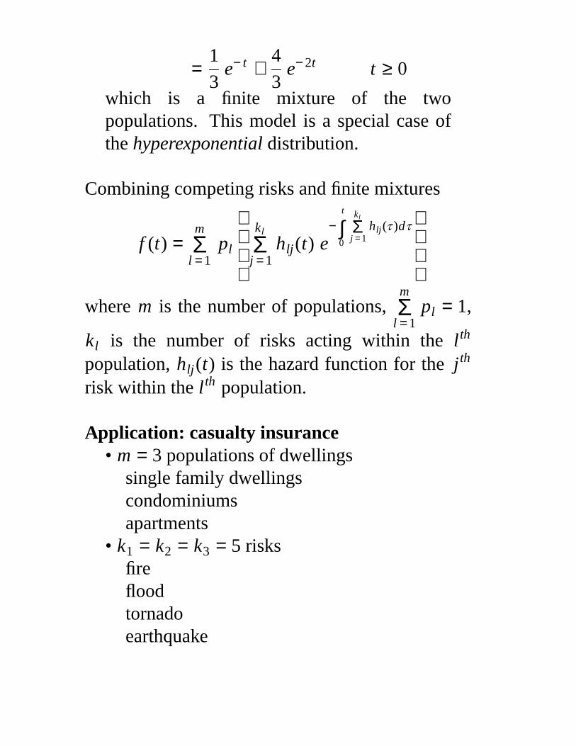
=1
3e− t +
4
3e− 2t t ≥ 0
which is a finite mixture of the twopopulations. This model is a special case ofthe hyperexponential distribution.
Combining competing risks and finite mixtures
f (t) =m
l = 1Σ pl
kl
j = 1Σ hlj(t) e
−t
0∫
kl
j = 1Σ hlj(τ )dτ
where m is the number of populations,m
l = 1Σ pl = 1,
kl is the number of risks acting within the l th
population, hlj(t) is the hazard function for the jth
risk within the l th population.
Application: casualty insurance• m = 3 populations of dwellings
single family dwellingscondominiumsapartments
• k1 = k2 = k3 = 5 risksfirefloodtornadoearthquake

burglary
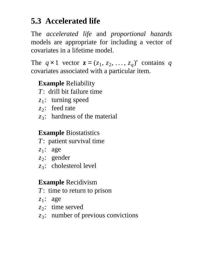
5.3 Accelerated life
The accelerated life and proportional hazardsmodels are appropriate for including a vector ofcovariates in a lifetime model.
The q × 1 vector z = (z1, z2, . . . , zq)′ contains qcovariates associated with a particular item.
Example ReliabilityT : drill bit failure timez1: turning speedz2: feed ratez3: hardness of the material
Example BiostatisticsT : patient survival timez1: agez2: genderz3: cholesterol level
Example RecidivismT : time to return to prisonz1: agez2: time servedz3: number of previous convictions
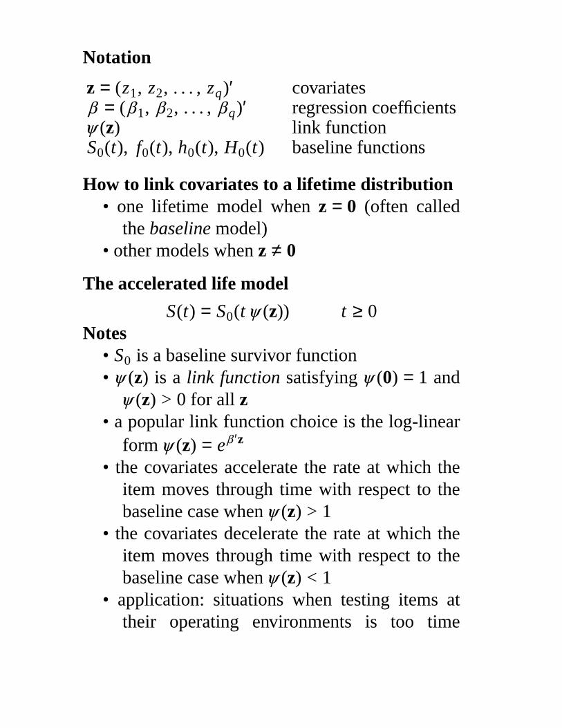
Notation
z = (z1, z2, . . . , zq)′ covariatesβ = (β 1, β 2, . . . , β q)′ regression coefficientsψ (z) link functionS0(t), f0(t), h0(t), H0(t) baseline functions
How to link covariates to a lifetime distribution• one lifetime model when z = 0 (often called
the baseline model)• other models when z ≠ 0
The accelerated life model
S(t) = S0(t ψ (z)) t ≥ 0Notes
• S0 is a baseline survivor function• ψ (z) is a link function satisfying ψ (0) = 1 and
ψ (z) > 0 for all z• a popular link function choice is the log-linear
form ψ (z) = eβ ′z
• the covariates accelerate the rate at which theitem moves through time with respect to thebaseline case when ψ (z) > 1
• the covariates decelerate the rate at which theitem moves through time with respect to thebaseline case when ψ (z) < 1
• application: situations when testing items attheir operating environments is too time
consuming
5.4 Proportional hazards
Whereas accelerated life models modify the ratethat the item moves through time based on thevalues of the covariates, proportional hazardsmodels modify the hazard function by the factorψ (z).
The proportional hazards model can be defined by
h(t) = ψ (z) h0(t).
Notes• the covariates increase the risk when ψ (z) > 1• the covariates decrease the risk when ψ (z) < 1• the log-linear form ψ (z) = eβ ′z is still an
appropriate choice for the link function
Table 5.1 Lifetime distribution representationsfor regression models.
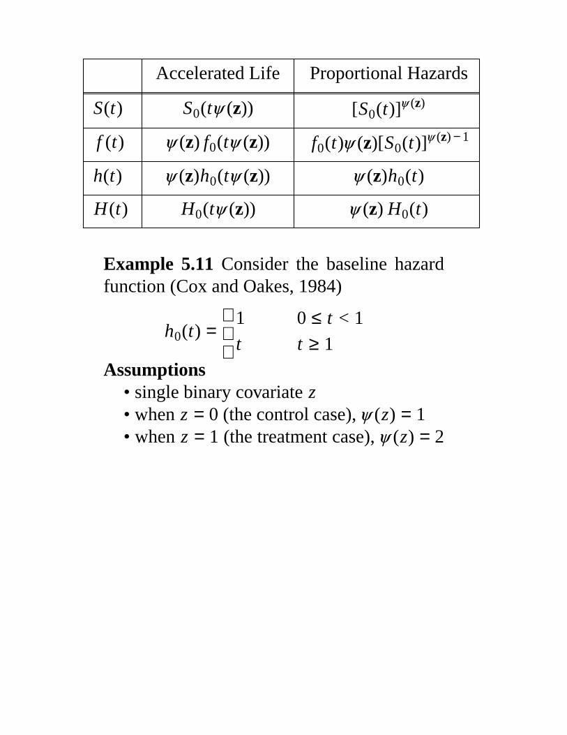
Accelerated Life Proportional Hazards
S(t) S0(tψ (z)) [S0(t)]ψ (z)
f (t) ψ (z) f0(tψ (z)) f0(t)ψ (z)[S0(t)]ψ (z) − 1
h(t) ψ (z)h0(tψ (z)) ψ (z)h0(t)
H(t) H0(tψ (z)) ψ (z) H0(t)
Example 5.11 Consider the baseline hazardfunction (Cox and Oakes, 1984)
h0(t) =
1
t
0 ≤ t < 1
t ≥ 1Assumptions
• single binary covariate z• when z = 0 (the control case), ψ (z) = 1• when z = 1 (the treatment case), ψ (z) = 2
0.0 0.5 1.0 1.5 2.0
0
1
2
3
4
h (t)0
h (t)PHh (t)AL
t
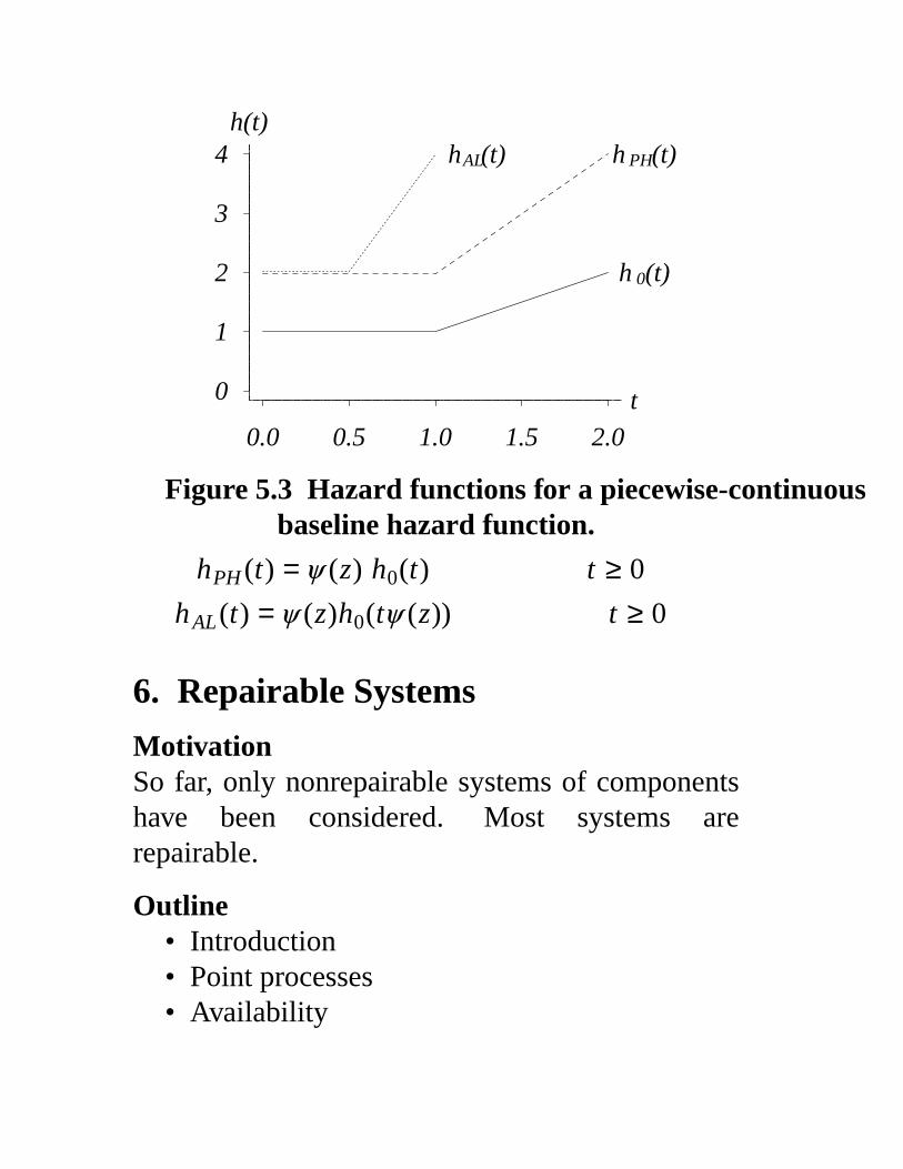
h(t)
Figure 5.3 Hazard functions for a piecewise-continuousbaseline hazard function.
hPH (t) = ψ (z) h0(t) t ≥ 0
hAL(t) = ψ (z)h0(tψ (z)) t ≥ 0
6. Repairable Systems
MotivationSo far, only nonrepairable systems of componentshave been considered. Most systems arerepairable.
Outline• Introduction• Point processes• Availability
• Birth-death processes
6.1 Introduction
A repairable item may be returned to an operatingcondition after failure to perform a requiredfunction by any method other than replacement ofthe entire item.
Replacement models• used when a nonrepairable item is replaced
with another item upon failure• "socket models"• unlimited spares• redundancy allocation problem (optimal
number of spares)• replacement policies
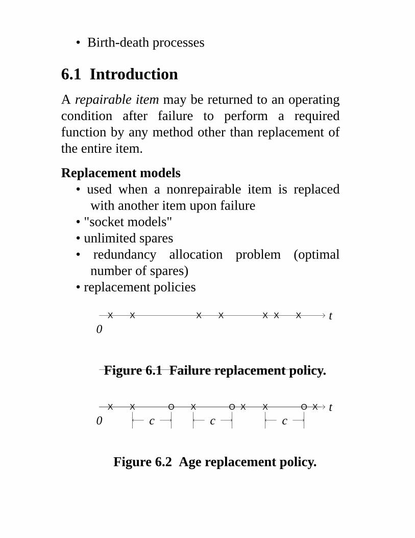
t0
X X X X X X X
Figure 6.1 Failure replacement policy.
t0
X X O X O X X O X
c c c
Figure 6.2 Age replacement policy.
t
0
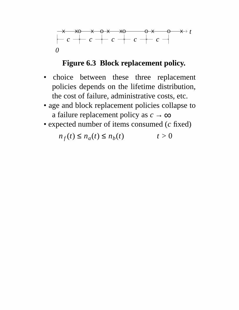
X XO X O X XO O X O X
c c c c c
Figure 6.3 Block replacement policy.
• choice between these three replacementpolicies depends on the lifetime distribution,the cost of failure, administrative costs, etc.
• age and block replacement policies collapse toa failure replacement policy as c → ∞
• expected number of items consumed (c fixed)
n f (t) ≤ na(t) ≤ nb(t) t > 0
6.2 Point processes
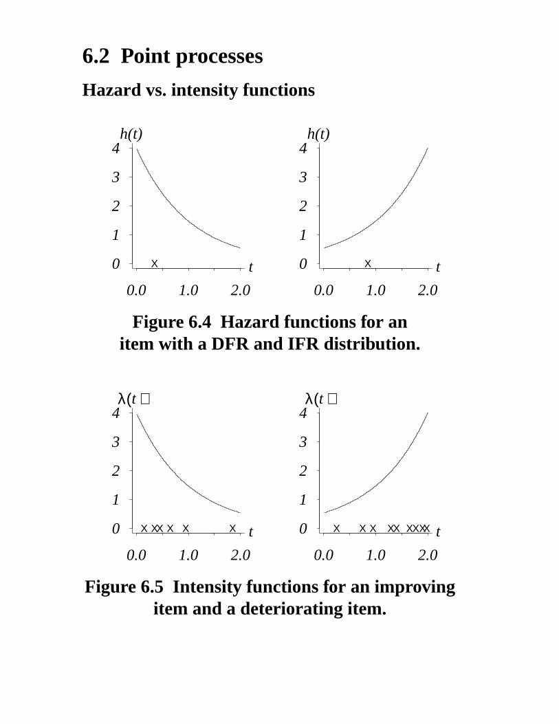
Hazard vs. intensity functions
0.0 1.0 2.0
0
1
2
3
4
X t
h(t)
0.0 1.0 2.0
0
1
2
3
4
X t
h(t)
Figure 6.4 Hazard functions for anitem with a DFR and IFR distribution.
0.0 1.0 2.0
0
1
2
3
4
X XX X X X t
λ( )t
0.0 1.0 2.0
0
1
2
3
4
X X X XX XXXX t
λ( )t
Figure 6.5 Intensity functions for an improvingitem and a deteriorating item.
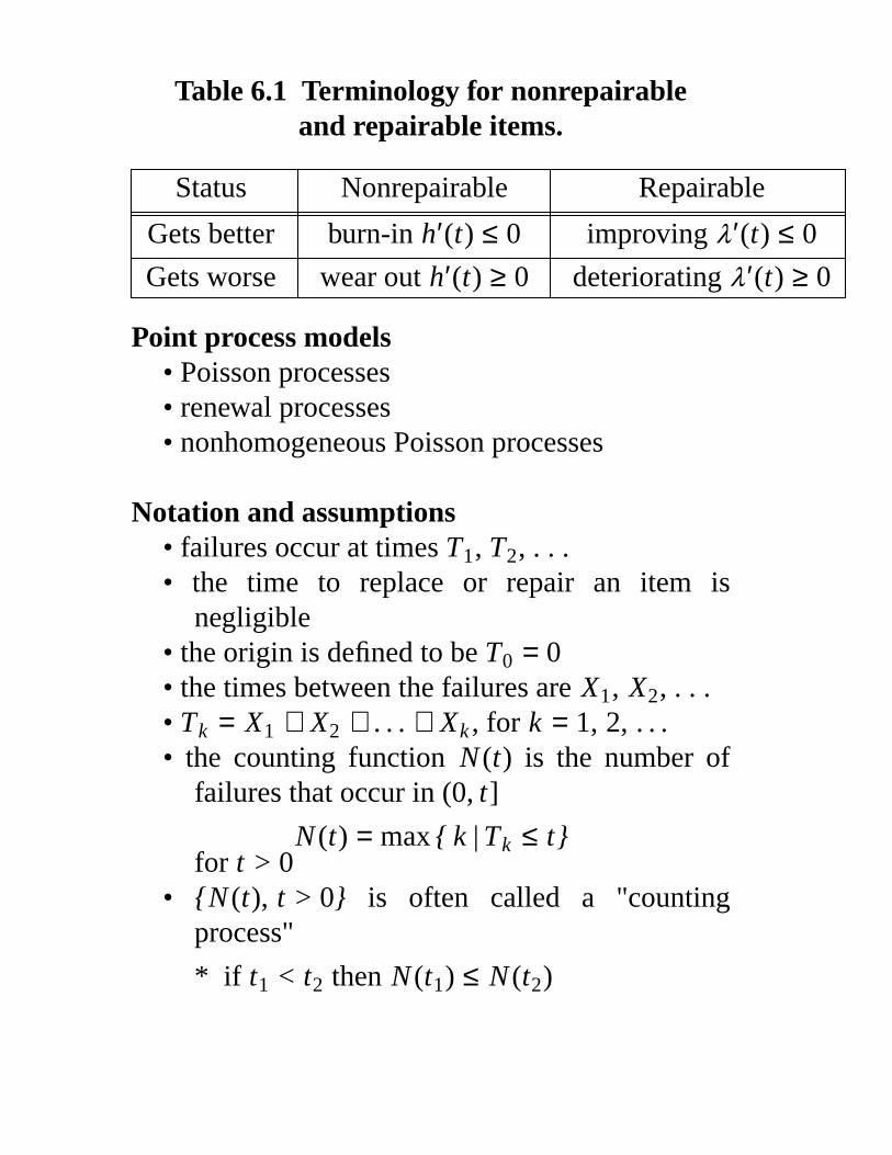
Table 6.1 Terminology for nonrepairableand repairable items.
Status Nonrepairable Repairable
Gets better burn-in h′(t) ≤ 0 improving λ ′(t) ≤ 0
Gets worse wear out h′(t) ≥ 0 deteriorating λ ′(t) ≥ 0
Point process models• Poisson processes• renewal processes• nonhomogeneous Poisson processes
Notation and assumptions• failures occur at times T1, T2, . . .• the time to replace or repair an item is
negligible• the origin is defined to be T0 = 0• the times between the failures are X1, X2, . . .• Tk = X1 + X2 + . . . + Xk , for k = 1, 2, . . .• the counting function N (t) is the number of
failures that occur in (0, t]
N (t) = max { k | Tk ≤ t}for t > 0
• {N (t), t > 0} is often called a "countingprocess"
* if t1 < t2 then N (t1) ≤ N (t2)
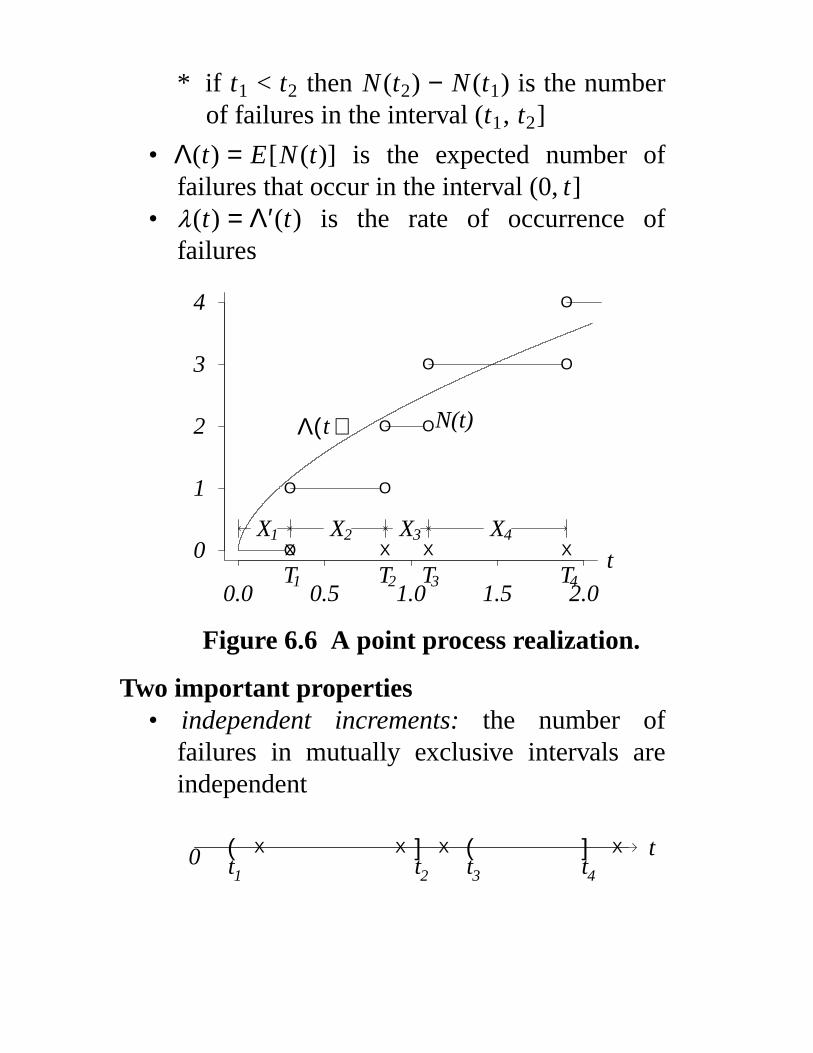
* if t1 < t2 then N (t2) − N (t1) is the numberof failures in the interval (t1, t2]
• Λ(t) = E[N (t)] is the expected number offailures that occur in the interval (0, t]
• λ(t) = Λ′(t) is the rate of occurrence offailures
0.0 0.5 1.0 1.5 2.0
0
1
2
3
4
tXOX1
T1
X
O O
X2
T2
X
O O
X3
T3
X
O O
X4
T4
O
N(t)Λ( )t
Figure 6.6 A point process realization.
Tw o important properties• independent increments: the number of
failures in mutually exclusive intervals areindependent
tX X X X( ] ( ]t t t t1 2 3 4
0
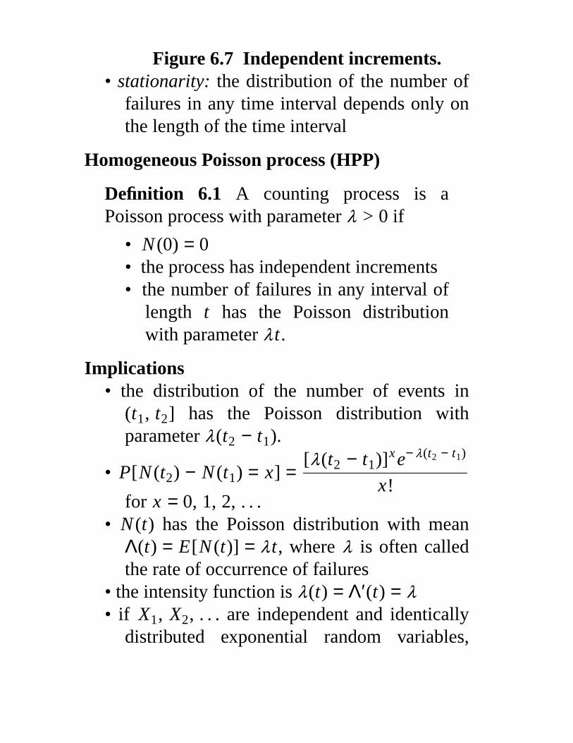
Figure 6.7 Independent increments.• stationarity: the distribution of the number of
failures in any time interval depends only onthe length of the time interval
Homogeneous Poisson process (HPP)
Definition 6.1 A counting process is aPoisson process with parameter λ > 0 if
• N (0) = 0• the process has independent increments• the number of failures in any interval of
length t has the Poisson distributionwith parameter λ t.
Implications• the distribution of the number of events in
(t1, t2] has the Poisson distribution withparameter λ(t2 − t1).
• P[N (t2) − N (t1) = x] =[λ(t2 − t1)]xe− λ(t2 − t1)
x!for x = 0, 1, 2, . . .
• N (t) has the Poisson distribution with meanΛ(t) = E[N (t)] = λ t, where λ is often calledthe rate of occurrence of failures
• the intensity function is λ(t) = Λ′(t) = λ• if X1, X2, . . . are independent and identically
distributed exponential random variables,

then N (t) corresponds to a Poisson process• this model is sometimes called just a Poisson
process
Nonhomogeneous Poisson process (NHPP)
Four reasons to consider an NHPP• the HPP is a special case of an NHPP
(stationarity assumption relaxed)• the probabilistic model for an NHPP is
mathematically tractable• the statistical methods for an NHPP are also
mathematically tractable• the NHPP is capable of modeling improving
and deteriorating systems
Intensity function: λ(t)
Cumulative intensity function: Λ(t) =t
0∫ λ(τ )dτ
Definition 6.4 A counting process is anonhomogeneous Poisson process withintensity function λ(t) ≥ 0 if
• N (0) = 0• the process has independent increments• the probability of exactly n ev ents
occurring in the interval (a, b] is giv enby
P[N (b) − N (a) = n] =[
b
a∫ λ(t)dt]n e
−b
a∫ λ(t)dt
n!for n = 0, 1, . . . .
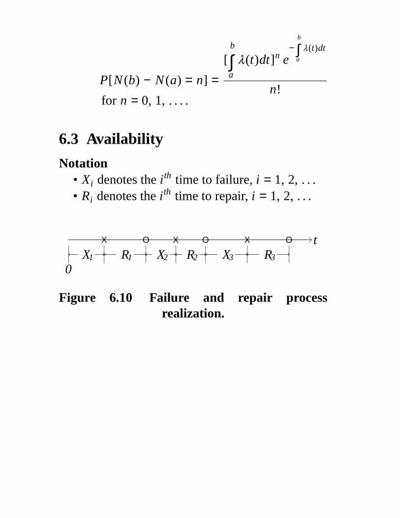
6.3 Availability
Notation• Xi denotes the ith time to failure, i = 1, 2, . . .• Ri denotes the ith time to repair, i = 1, 2, . . .
t
0
X O X O X O
R1 R2 R3X1 X2 X3
Figure 6.10 Failure and repair processrealization.
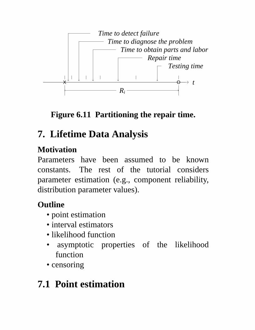
tX O
Time to detect failureTime to diagnose the problem
Time to obtain parts and laborRepair time
Testing time
Ri
Figure 6.11 Partitioning the repair time.
7. Lifetime Data Analysis
MotivationParameters have been assumed to be knownconstants. The rest of the tutorial considersparameter estimation (e.g., component reliability,distribution parameter values).
Outline• point estimation• interval estimators• likelihood function• asymptotic properties of the likelihood
function• censoring
7.1 Point estimation
A point estimator is a statistic used to estimate apopulation parameter.
Definition 7.1 The point estimator θ is anunbiased estimator of θ if and only ifE[θ ] =θ .
Definition 7.2 Let θ1 and θ2 be two unbiasedpoint estimators of the parameter θ . Then
V (θ1)
V (θ2)is the efficiency of θ1 relative to θ2.
7.2 Interval estimation
Confidence intervals give bounds that contain apopulation parameter with a prescribed probability
L ≤ θ ≤ UNotes
• L and U are functions ofthe sample size nthe lifetimes t1, . . . , tn
the nominal coverage of the interval 1 − α• true value of the parameter θ is denoted by θ 0
• popular choices for α are 0.10 and 0.05• confidence intervals: exact, approximate,
asymptotically exact

0.0 0.5 1.0 1.5 2.0 2.5θθ0
( )O θ( )O θ
( )O θ( )O θ( )O θ
( )O θ( )O θ
( )O θ( )O θ
( )O θ
Figure 7.2 Ten 90% confidence intervals for θ (n = 25).
7.3 Likelihood theory
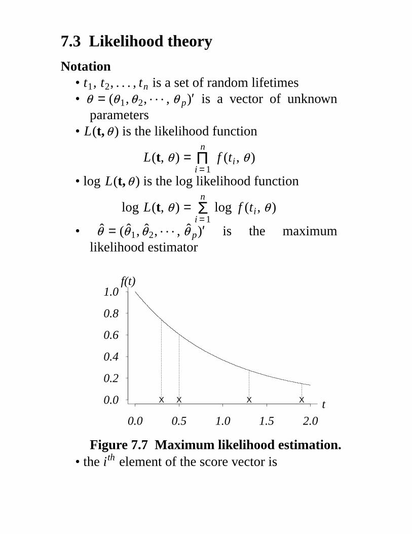
Notation• t1, t2, . . . , tn is a set of random lifetimes• θ = (θ 1,θ2, . . . , θ p)′ is a vector of unknown
parameters• L(t,θ ) is the likelihood function
L(t, θ ) =n
i = 1Π f (ti , θ )
• log L(t,θ ) is the log likelihood function
log L(t, θ ) =n
i = 1Σ log f (ti , θ )
• θ = (θ1, θ2, . . . , θ p)′ is the maximumlikelihood estimator
0.0 0.5 1.0 1.5 2.0
0.0
0.2
0.4
0.6
0.8
1.0
X X X X t
f(t)
Figure 7.7 Maximum likelihood estimation.• the ith element of the score vector is
Ui (θ ) =∂ log L(t,θ )
∂θ ii = 1, 2, . . . , p
• the score vector components have expectation
E [Ui (θ ) ] = 0 i = 1, 2, . . . , p
and variance-covariance matrix
I (θ ) = E[U (θ ) U′ (θ )]
• this variance-covariance matrix is called theFisher information matrix with components
Cov(Ui (θ ),U j (θ )) = E
− ∂2 log L(t,θ )
∂θ i ∂θ j
for i = 1, 2, . . . , p and j = 1, 2, . . . , p.• the observed information matrix has
components O(θ ) is
− ∂2 log L(t, θ )
∂θ i ∂θ j
θ = θ
i = 1, 2, . . . , p
j = 1, 2, . . . , p
Example 7.7 Collect t1, t2, . . . , tn from anexponential population with a singleparameter θ
f (t;θ ) =1
θe− t /θ t > 0
The likelihood function is
L (t,θ ) =n
i = 1Π f (ti , θ )
=n
i = 1Π
1
θe− ti /θ
= θ − n e−
n
i = 1Σ ti /θ
The log likelihood function is
log L(t,θ ) = − n logθ −n
i = 1Σ ti /θ
The score vector is
U(θ ) =∂ log L(t,θ )
∂θ= −
n
θ+
n
i = 1Σ ti
θ 2
The maximum likelihood estimator is
θ =1
n
n
i = 1Σ ti
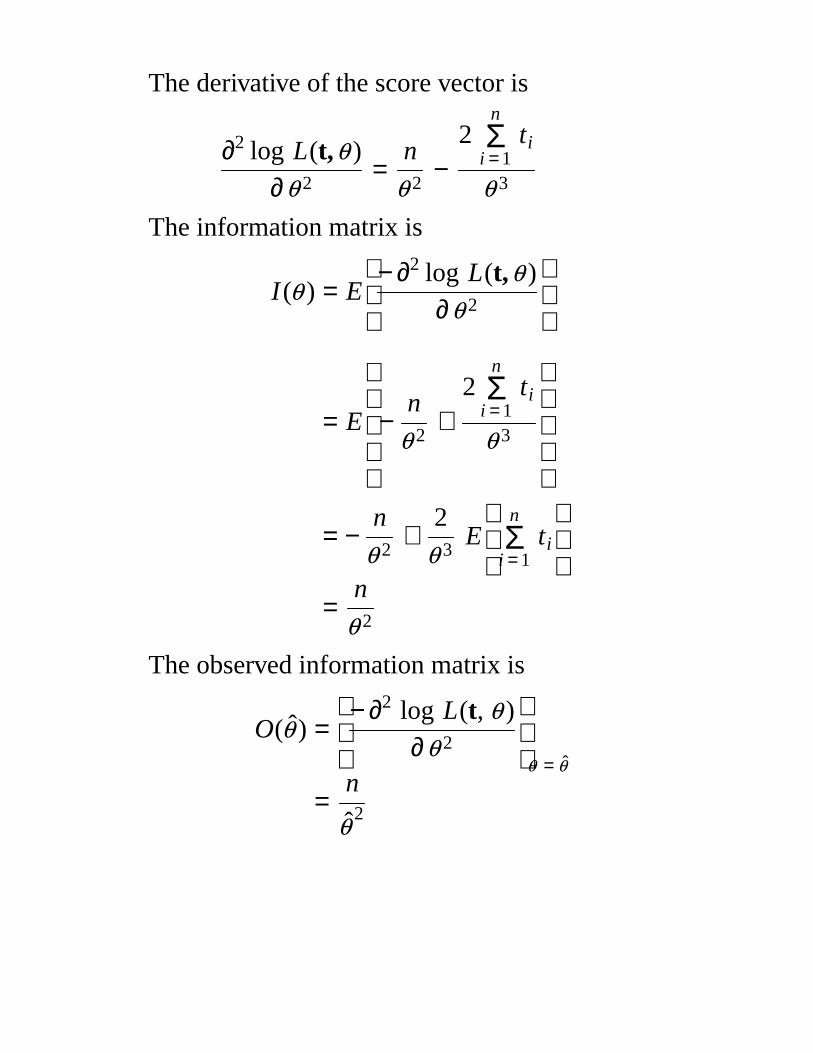
The derivative of the score vector is
∂2 log L(t,θ )
∂θ 2=
n
θ 2−
2n
i = 1Σ ti
θ 3
The information matrix is
I (θ ) = E
− ∂2 log L(t,θ )
∂θ 2
= E
−n
θ 2+
2n
i = 1Σ ti
θ 3
= −n
θ 2+
2
θ 3E
n
i = 1Σ ti
=n
θ 2
The observed information matrix is
O(θ ) =
− ∂2 log L(t, θ )
∂θ 2
θ = θ
=n
θ 2
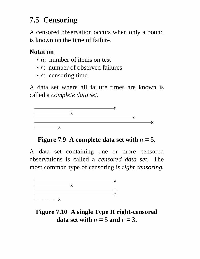
7.5 Censoring
A censored observation occurs when only a boundis known on the time of failure.
Notation• n: number of items on test• r: number of observed failures• c: censoring time
A data set where all failure times are known iscalled a complete data set.
XX
XX
X
Figure 7.9 A complete data set with n = 5.
A data set containing one or more censoredobservations is called a censored data set. Themost common type of censoring is right censoring.
XOO
XX
Figure 7.10 A single Type II right-censoreddata set with n = 5 and r = 3.
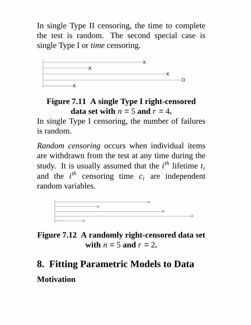
In single Type II censoring, the time to completethe test is random. The second special case issingle Type I or time censoring.
XO
XX
X
Figure 7.11 A single Type I right-censoreddata set with n = 5 and r = 4.
In single Type I censoring, the number of failuresis random.
Random censoring occurs when individual itemsare withdrawn from the test at any time during thestudy. It is usually assumed that the ith lifetime ti
and the ith censoring time ci are independentrandom variables.
O
X
O
O
X
Figure 7.12 A randomly right-censored data setwith n = 5 and r = 2.
8. Fitting Parametric Models to Data
Motivation
Find point and interval estimators for theexponential and Weibull distributions for sampledata sets.
Outline• sample data sets• exponential distribution• Weibull distribution
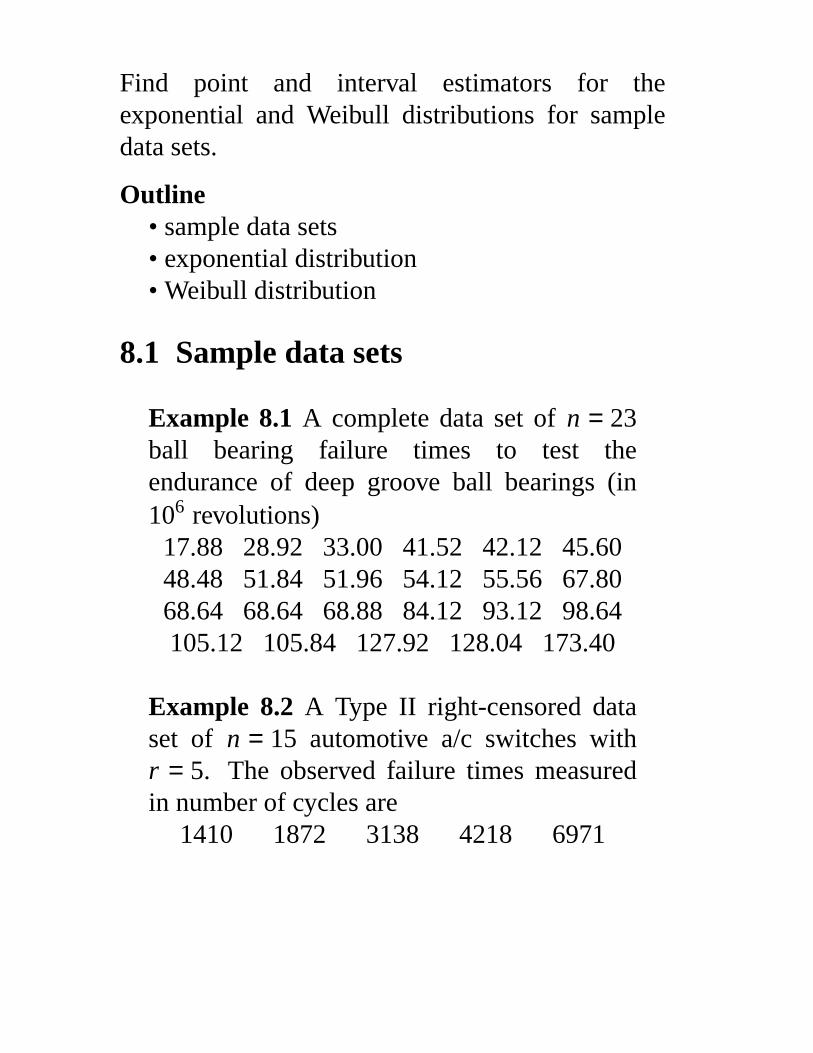
8.1 Sample data sets
Example 8.1 A complete data set of n = 23ball bearing failure times to test theendurance of deep groove ball bearings (in106 revolutions)
17.88 28.92 33.00 41.52 42.12 45.6048.48 51.84 51.96 54.12 55.56 67.8068.64 68.64 68.88 84.12 93.12 98.64105.12 105.84 127.92 128.04 173.40
Example 8.2 A Type II right-censored dataset of n = 15 automotive a/c switches withr = 5. The observed failure times measuredin number of cycles are
1410 1872 3138 4218 6971
Example 8.3 Determine the effect of 6-MP(6-mercaptopurine) on leukemia remissiontimes. A sample of n = 21 patients weretreated with 6-MP, and r = 9 remission timeswere observed. The survival times (inweeks) are6 6 6 6* 7 9* 10 10* 11* 13 16 17*19* 20* 22 23 25* 32* 32* 34* 35*
Control group: 21 other leukemia patients1 1 2 2 3 4 4 5 5 8 8
8 8 11 11 12 12 15 17 22 23
Example 8.4 Forty motorettes were placedon test at 150oC, 170oC, 190oC and 220oC(ten motorettes at each temperature level andType I censoring). The failure times (inhours) are150oC: 8064* 8064* 8064* 8064*8064* 8064* 8064* 8064* 8064* 8064*170oC: 1764 2772 3444 3542 3780
4860 5196 5448* 5448* 5448*190oC: 408 408 1344 1344 1440 1680*
1680* 1680* 1680* 1680*220oC: 408 408 504 504 504 528*
528* 528* 528* 528*Failure times are the midpoint of an

inspection period. Operating temperature:130oC.
8.2 The exponential distribution
Goal: find point and interval estimates for thep = 1 parameter λ .
The exponential distribution can be parameterizedby either its failure rate λ or its meanµ = θ = 1 / λ .
S(t, λ) = e− λ t f (t, λ) = λe− λ t
h(t, λ) = λ H(t, λ) = λ tfor all t ≥ 0.
Complete data sets
A complete data set consists of failure timest1, t2, . . . , tn.
L(λ) =n
i = 1Π f (ti , λ)
The log likelihood function is
log L(λ) =n
i = 1Σ [log h(ti , λ) − H(ti , λ)]
or
log L(λ) =n
i = 1Σ [log λ − λ ti] = n log λ − λ
n
i = 1Σ ti
The single element score vector is
U(λ) =∂ log L(λ)
∂λ=
n
λ−
n
i = 1Σ ti
The MLE is λ =n
n
i = 1Σ ti
Exact confidence intervals for λ
λ χ 22n, 1 − α / 2
2n< λ <
λ χ 22n, α / 2
2n
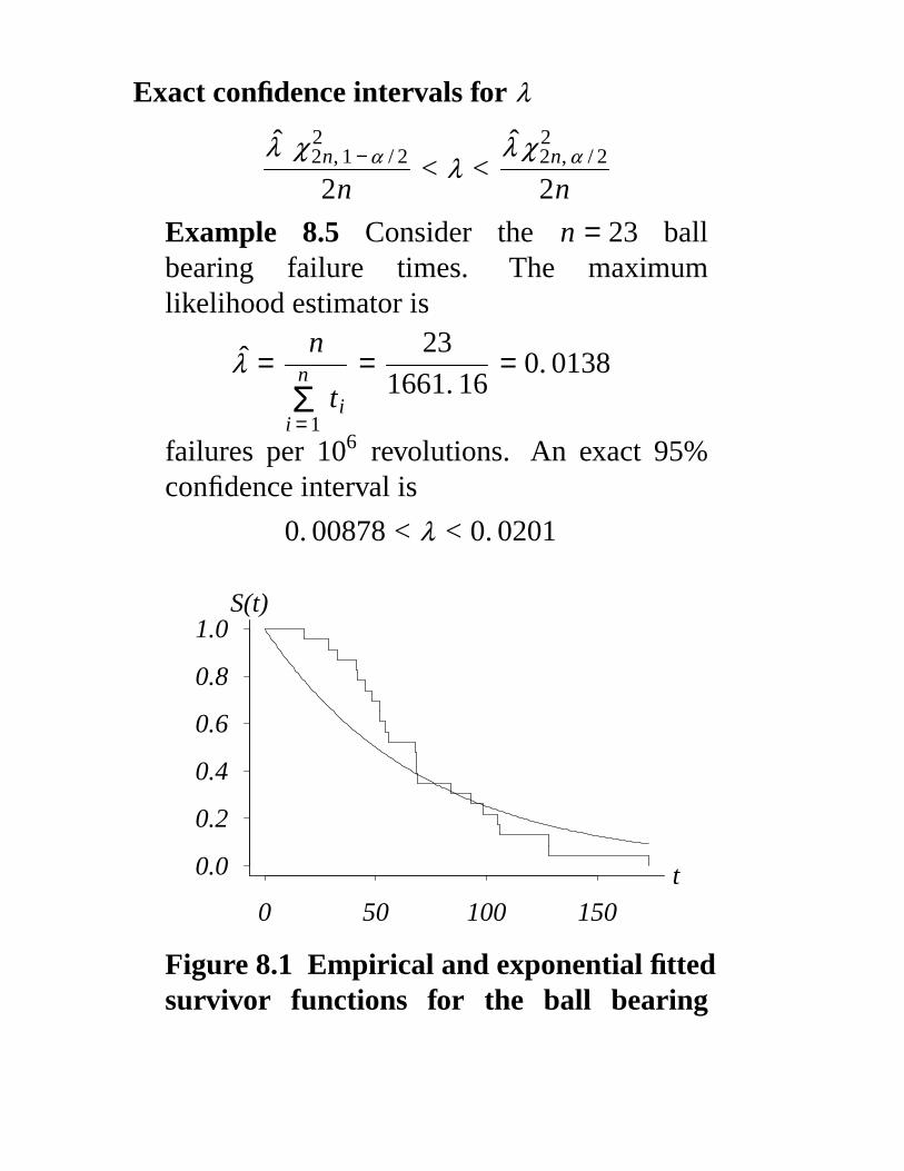
Example 8.5 Consider the n = 23 ballbearing failure times. The maximumlikelihood estimator is
λ =n
n
i = 1Σ ti
=23
1661. 16= 0. 0138
failures per 106 revolutions. An exact 95%confidence interval is
0. 00878 < λ < 0. 0201
0 50 100 150
0.0
0.2
0.4
0.6
0.8
1.0
t
S(t)
Figure 8.1 Empirical and exponential fittedsurvivor functions for the ball bearing
data set.
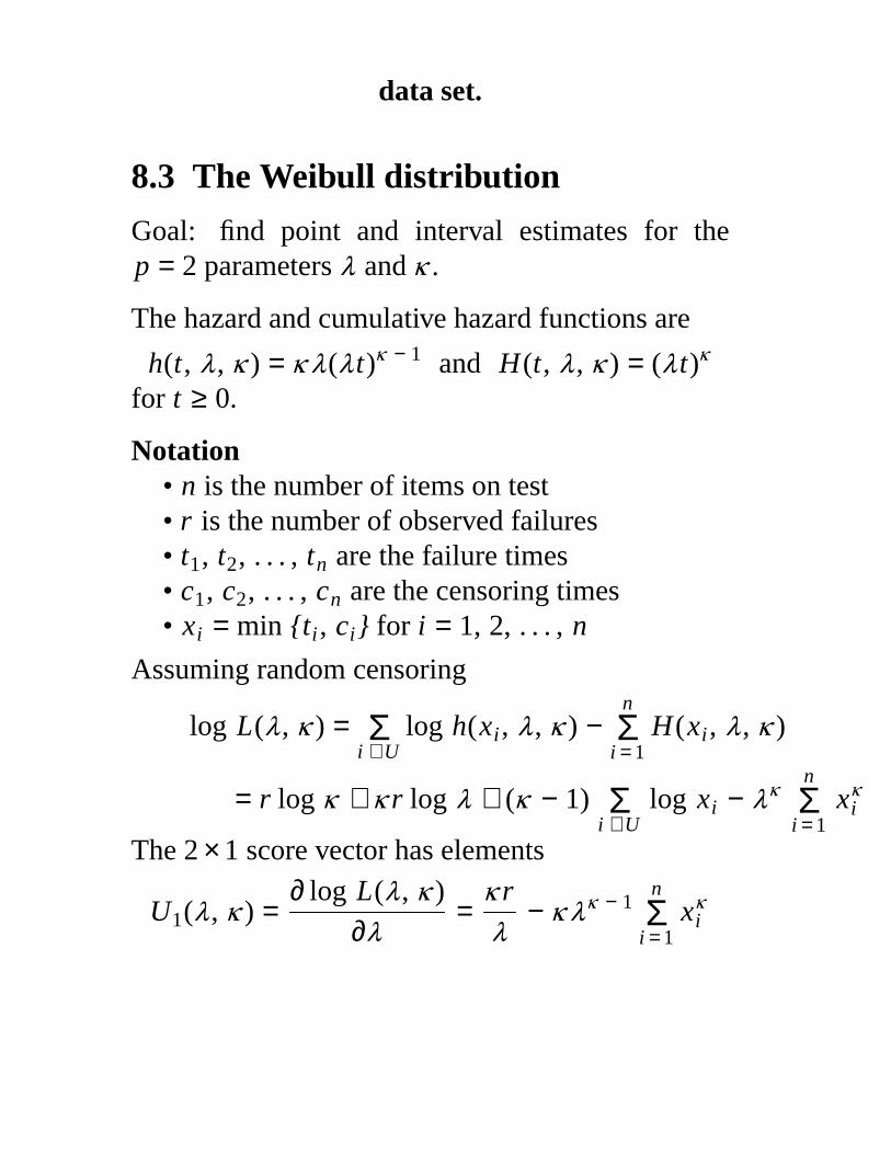
8.3 The Weibull distribution
Goal: find point and interval estimates for thep = 2 parameters λ and κ .
The hazard and cumulative hazard functions are
h(t, λ , κ ) = κ λ(λ t)κ − 1 and H(t, λ , κ ) = (λ t)κ
for t ≥ 0.
Notation• n is the number of items on test• r is the number of observed failures• t1, t2, . . . , tn are the failure times• c1, c2, . . . , cn are the censoring times• xi = min {ti , ci} for i = 1, 2, . . . , n
Assuming random censoring
log L(λ , κ ) =i ∈UΣ log h(xi , λ , κ ) −
n
i = 1Σ H(xi , λ , κ )
= r log κ + κ r log λ + (κ − 1)i ∈UΣ log xi − λκ
n
i = 1Σ xκ
i
The 2 × 1 score vector has elements
U1(λ , κ ) =∂ log L(λ , κ )
∂λ=
κ r
λ− κ λκ − 1
n
i = 1Σ xκ
i
U2(λ , κ ) =∂ log L(λ , κ )
∂κ=
r
κ+ r log λ +
i ∈UΣ log xi −
n
i = 1Σ (λ xi)
κ log λ xi
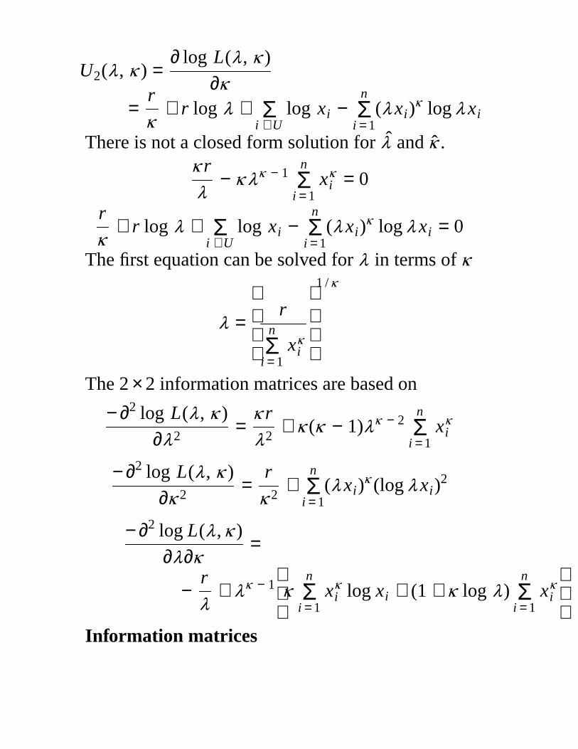
There is not a closed form solution for λ and κ .κ r
λ− κ λκ − 1
n
i = 1Σ xκ
i = 0
r
κ+ r log λ +
i ∈UΣ log xi −
n
i = 1Σ (λ xi)
κ log λ xi = 0
The first equation can be solved for λ in terms of κ
λ =
rn
i = 1Σ xκ
i
1 /κ
The 2 × 2 information matrices are based on
− ∂2 log L(λ , κ )
∂λ2=
κ r
λ2+ κ (κ − 1)λκ − 2
n
i = 1Σ xκ
i
− ∂2 log L(λ , κ )
∂κ 2=
r
κ 2+
n
i = 1Σ (λ xi)
κ (log λ xi)2
− ∂2 log L(λ ,κ )
∂λ∂κ=
−r
λ+ λκ − 1
κ
n
i = 1Σ xκ
i log xi + (1 + κ log λ)n
i = 1Σ xκ
i
Information matrices
• the expected values of these quantities are nottractable
• use λ and κ to obtain the observed informationmatrix
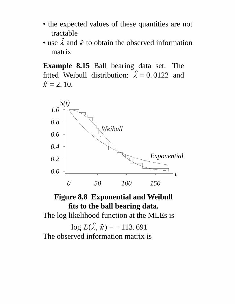
Example 8.15 Ball bearing data set. Thefitted Weibull distribution: λ = 0. 0122 andκ = 2. 10.
0 50 100 150
0.0
0.2
0.4
0.6
0.8
1.0
t
S(t)
Weibull
Exponential
Figure 8.8 Exponential and Weibullfits to the ball bearing data.
The log likelihood function at the MLEs is
log L(λ , κ ) = − 113. 691The observed information matrix is
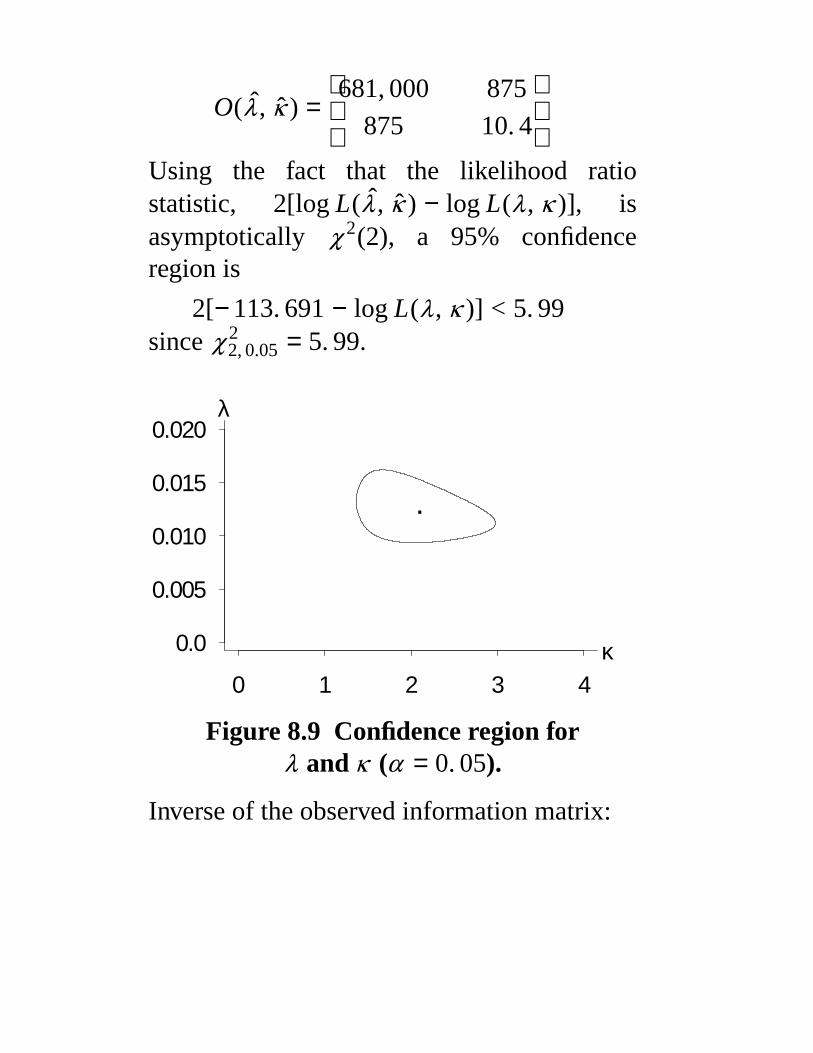
O(λ , κ ) =
681, 000
875
875
10. 4
Using the fact that the likelihood ratiostatistic, 2[log L(λ , κ ) − log L(λ , κ )], isasymptotically χ 2(2), a 95% confidenceregion is
2[− 113. 691 − log L(λ , κ )] < 5. 99since χ 2
2, 0.05 = 5. 99.
0 1 2 3 4
0.0
0.005
0.010
0.015
0.020
.
λ
κ
Figure 8.9 Confidence region forλ and κ (α = 0. 05).
Inverse of the observed information matrix:
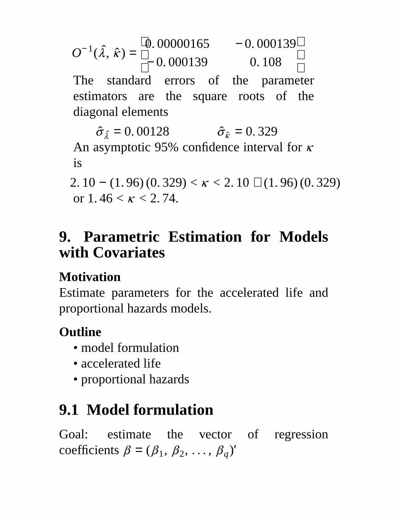
O− 1(λ , κ ) =
0. 00000165
− 0. 000139
− 0. 000139
0. 108
The standard errors of the parameterestimators are the square roots of thediagonal elements
σ λ = 0. 00128 σ κ = 0. 329An asymptotic 95% confidence interval for κis
2. 10 − (1. 96) (0. 329) < κ < 2. 10 + (1. 96) (0. 329)or 1. 46 < κ < 2. 74.
9. Parametric Estimation for Modelswith Covariates
MotivationEstimate parameters for the accelerated life andproportional hazards models.
Outline• model formulation• accelerated life• proportional hazards
9.1 Model formulation
Goal: estimate the vector of regressioncoefficients β = (β 1, β 2, . . . , β q)′
Applications• determine which covariates significantly
impact survival• determine the impact of changing the values of
covariates
The accelerated life model
S(t, z) = S0(t ψ (z))
The proportional hazards model
h(t, z) = ψ (z) h0(t)
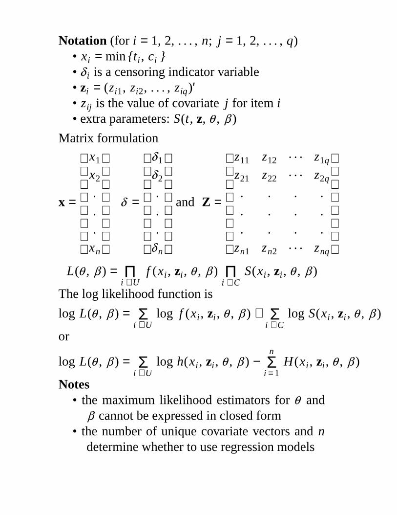
Notation (for i = 1, 2, . . . , n; j = 1, 2, . . . , q)• xi = min {ti , ci }• δ i is a censoring indicator variable• zi = (zi1, zi2, . . . , ziq)′• zij is the value of covariate j for item i• extra parameters: S(t, z, θ , β )
Matrix formulation
x =
x1
x2
.
.
.
xn
δ =
δ1
δ2
.
.
.
δ n
and Z =
z11
z21
.
.
.
zn1
z12
z22
.
.
.
zn2
. . .
. . .
.
.
.. . .
z1q
z2q
.
.
.
znq
L(θ , β ) =i ∈UΠ f (xi , zi , θ , β )
i ∈CΠ S(xi , zi , θ , β )
The log likelihood function is
log L(θ , β ) =i ∈UΣ log f (xi , zi , θ , β ) +
i ∈CΣ log S(xi , zi , θ , β )
or
log L(θ , β ) =i ∈UΣ log h(xi , zi , θ , β ) −
n
i = 1Σ H(xi , zi , θ , β )
Notes• the maximum likelihood estimators for θ and
β cannot be expressed in closed form• the number of unique covariate vectors and n
determine whether to use regression models
9.3 Proportional hazards
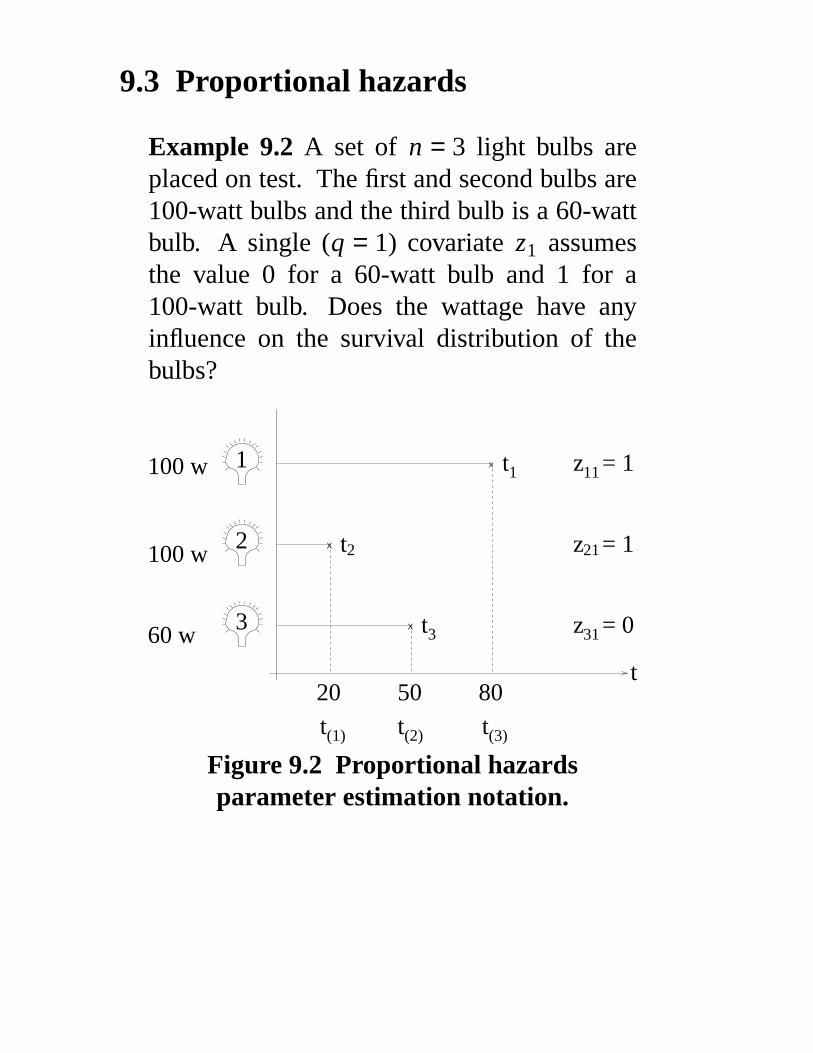
Example 9.2 A set of n = 3 light bulbs areplaced on test. The first and second bulbs are100-watt bulbs and the third bulb is a 60-wattbulb. A single (q = 1) covariate z1 assumesthe value 0 for a 60-watt bulb and 1 for a100-watt bulb. Does the wattage have anyinfluence on the survival distribution of thebulbs?
X
X
X
100 w
100 w
60 w
1
2
3
20 50 80t
t
t
t
t t t(1) (2) (3)
1
2
3
z = 1
z = 1
z = 0
11
21
31
Figure 9.2 Proportional hazardsparameter estimation notation.
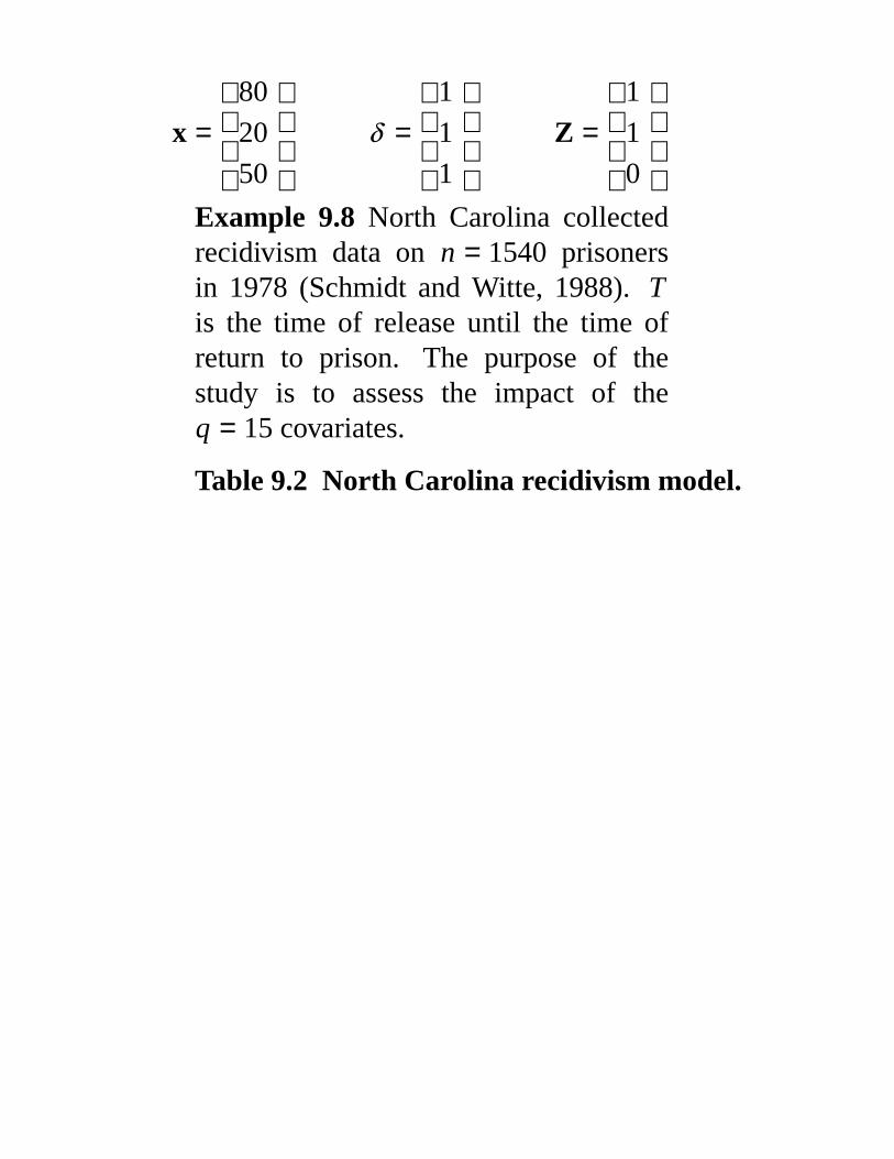
x =
80
20
50
δ =
1
1
1
Z =
1
1
0
Example 9.8 North Carolina collectedrecidivism data on n = 1540 prisonersin 1978 (Schmidt and Witte, 1988). Tis the time of release until the time ofreturn to prison. The purpose of thestudy is to assess the impact of theq = 15 covariates.
Table 9.2 North Carolina recidivism model.
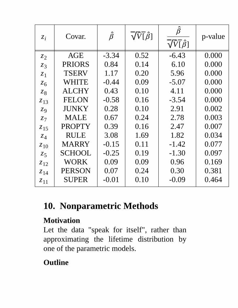
zi Covar. β √ V [β ]β
√ V [β ]p-value
z2 AGE -3.34 0.52 -6.43 0.000z3 PRIORS 0.84 0.14 6.10 0.000z1 TSERV 1.17 0.20 5.96 0.000z6 WHITE -0.44 0.09 -5.07 0.000z8 ALCHY 0.43 0.10 4.11 0.000z13 FELON -0.58 0.16 -3.54 0.000z9 JUNKY 0.28 0.10 2.91 0.002z7 MALE 0.67 0.24 2.78 0.003z15 PROPTY 0.39 0.16 2.47 0.007z4 RULE 3.08 1.69 1.82 0.034z10 MARRY -0.15 0.11 -1.42 0.077z5 SCHOOL -0.25 0.19 -1.30 0.097z12 WORK 0.09 0.09 0.96 0.169z14 PERSON 0.07 0.24 0.30 0.381z11 SUPER -0.01 0.10 -0.09 0.464
10. Nonparametric Methods
MotivationLet the data "speak for itself", rather thanapproximating the lifetime distribution byone of the parametric models.
Outline
• nonparametric estimates of the survivorfunction
• life tables
10.1 Survivor function estimation
0 50 100 150
0.0
0.2
0.4
0.6
0.8
1.0
Exponential fit
Nonparametric estimator
Population survivor function
t
S(t)
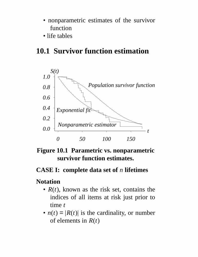
Figure 10.1 Parametric vs. nonparametricsurvivor function estimates.
CASE I: complete data set of n lifetimes
Notation• R(t), known as the risk set, contains the
indices of all items at risk just prior totime t
• n(t) = |R(t)| is the cardinality, or numberof elements in R(t)
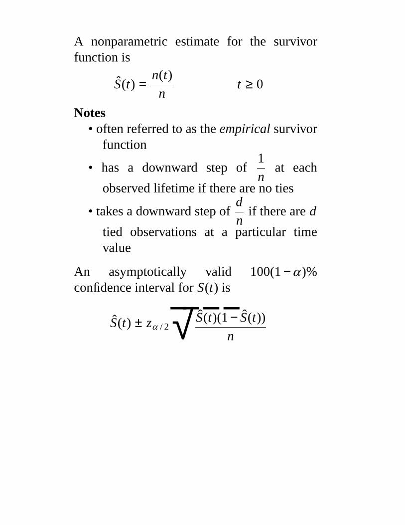
A nonparametric estimate for the survivorfunction is
S(t) =n(t)
nt ≥ 0
Notes• often referred to as the empirical survivor
function
• has a downward step of1
nat each
observed lifetime if there are no ties
• takes a downward step ofd
nif there are d
tied observations at a particular timevalue
An asymptotically valid 100(1 − α )%confidence interval for S(t) is
S(t) ± zα / 2√ S(t)(1 − S(t))
n
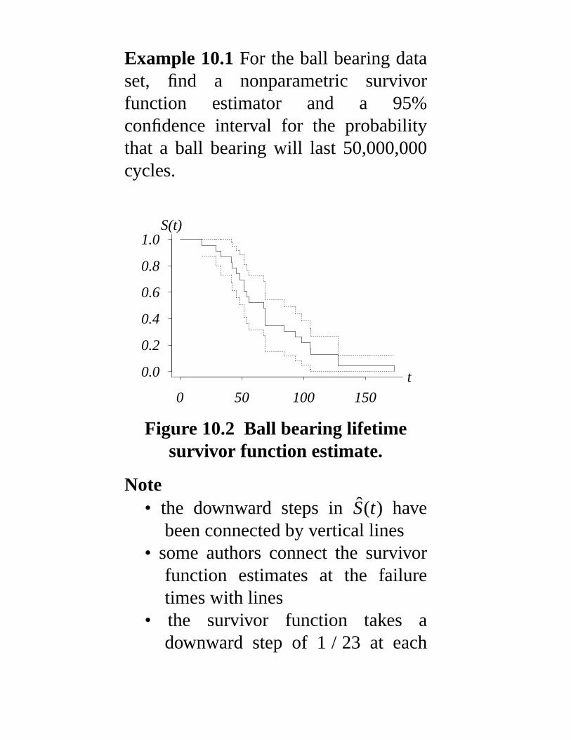
Example 10.1 For the ball bearing dataset, find a nonparametric survivorfunction estimator and a 95%confidence interval for the probabilitythat a ball bearing will last 50,000,000cycles.
0 50 100 150
0.0
0.2
0.4
0.6
0.8
1.0
t
S(t)
Figure 10.2 Ball bearing lifetimesurvivor function estimate.
Note• the downward steps in S(t) hav e
been connected by vertical lines• some authors connect the survivor
function estimates at the failuretimes with lines
• the survivor function takes adownward step of 1 / 23 at each

data value except 68.64, where ittakes a downward step of 2 / 23
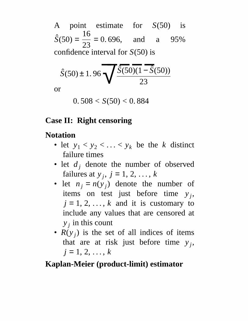
A point estimate for S(50) is
S(50) =16
23= 0. 696, and a 95%
confidence interval for S(50) is
S(50) ± 1. 96√ S(50)(1 − S(50))
23or
0. 508 < S(50) < 0. 884
Case II: Right censoring
Notation• let y1 < y2 < . . . < yk be the k distinct
failure times• let d j denote the number of observed
failures at y j , j = 1, 2, . . . , k• let n j = n(y j) denote the number of
items on test just before time y j ,j = 1, 2, . . . , k and it is customary toinclude any values that are censored aty j in this count
• R(y j) is the set of all indices of itemsthat are at risk just before time y j ,j = 1, 2, . . . , k
Kaplan-Meier (product-limit) estimator
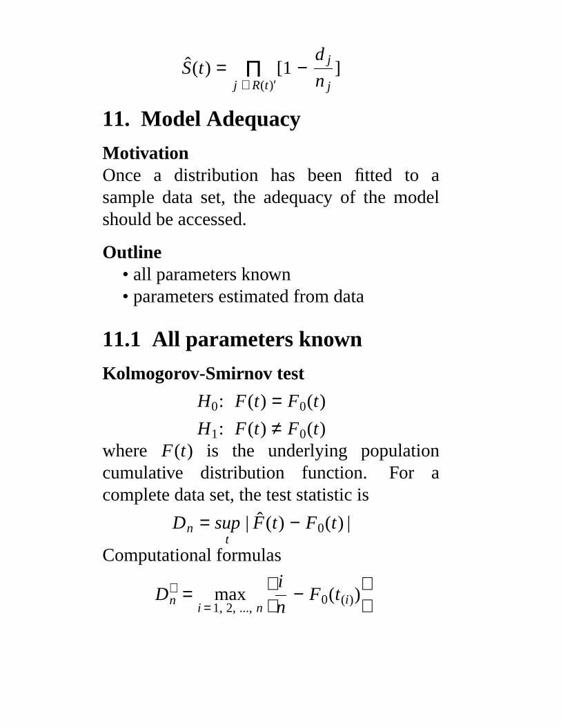
S(t) =j ∈ R(t)′
Π [1 −d j
n j]
11. Model Adequacy
MotivationOnce a distribution has been fitted to asample data set, the adequacy of the modelshould be accessed.
Outline• all parameters known• parameters estimated from data
11.1 All parameters known
Kolmogorov-Smirnov test
H0: F(t) = F0(t)
H1: F(t) ≠ F0(t)where F(t) is the underlying populationcumulative distribution function. For acomplete data set, the test statistic is
Dn =t
sup | F(t) − F0(t) |
Computational formulas
D+n =
i = 1, 2, ..., nmax
i
n− F0(t(i))
D−n =
i = 1, 2, ..., nmax
F0(t(i)) −
i − 1
n
Dn = max {D+n, D−
n }
0 50 100 150
0.0
0.2
0.4
0.6
0.8
1.0
D23
Exponential fit
Nonparametric estimator
t
S(t)
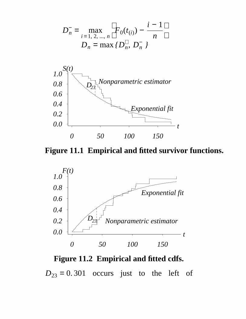
Figure 11.1 Empirical and fitted survivor functions.
0 50 100 150
0.0
0.2
0.4
0.6
0.8
1.0
D23
Exponential fit
Nonparametric estimator
t
F(t)
Figure 11.2 Empirical and fitted cdfs.
D23 = 0. 301 occurs just to the left of
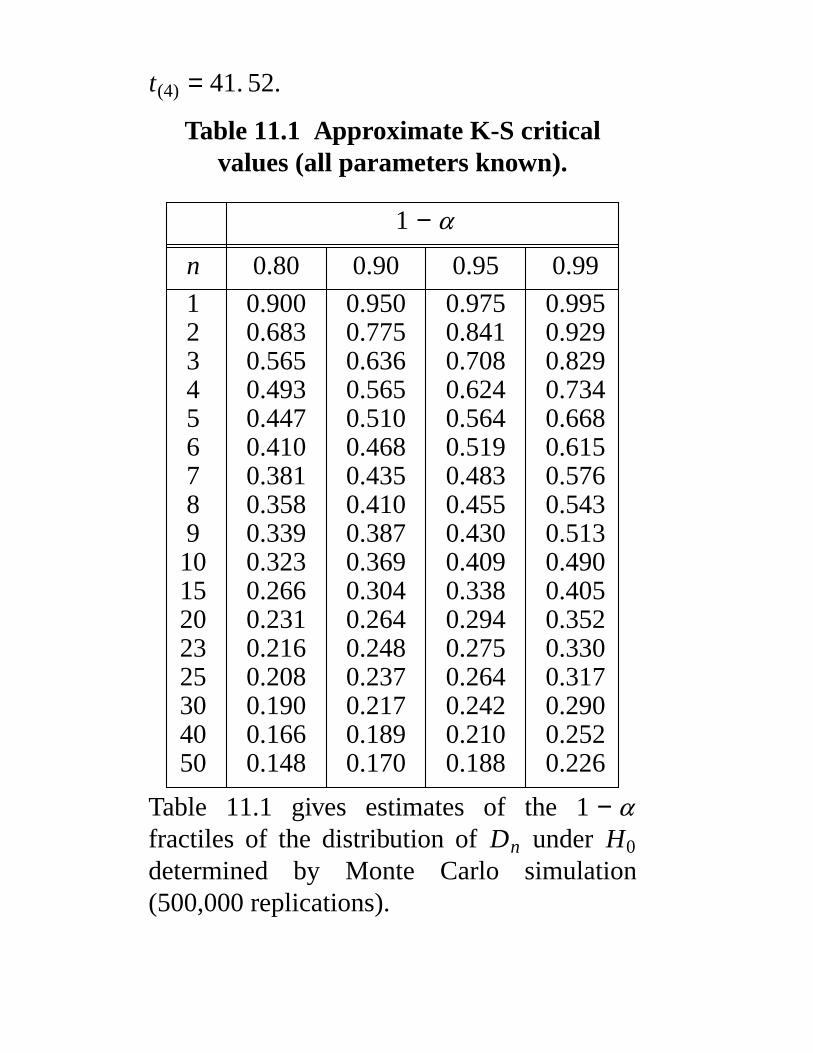
t(4) = 41. 52.
Table 11.1 Approximate K-S criticalvalues (all parameters known).
1 − α
n 0.80 0.90 0.95 0.99
1 0.900 0.950 0.975 0.9952 0.683 0.775 0.841 0.9293 0.565 0.636 0.708 0.8294 0.493 0.565 0.624 0.7345 0.447 0.510 0.564 0.6686 0.410 0.468 0.519 0.6157 0.381 0.435 0.483 0.5768 0.358 0.410 0.455 0.5439 0.339 0.387 0.430 0.51310 0.323 0.369 0.409 0.49015 0.266 0.304 0.338 0.40520 0.231 0.264 0.294 0.35223 0.216 0.248 0.275 0.33025 0.208 0.237 0.264 0.31730 0.190 0.217 0.242 0.29040 0.166 0.189 0.210 0.25250 0.148 0.170 0.188 0.226
Table 11.1 gives estimates of the 1 − αfractiles of the distribution of Dn under H0
determined by Monte Carlo simulation(500,000 replications).
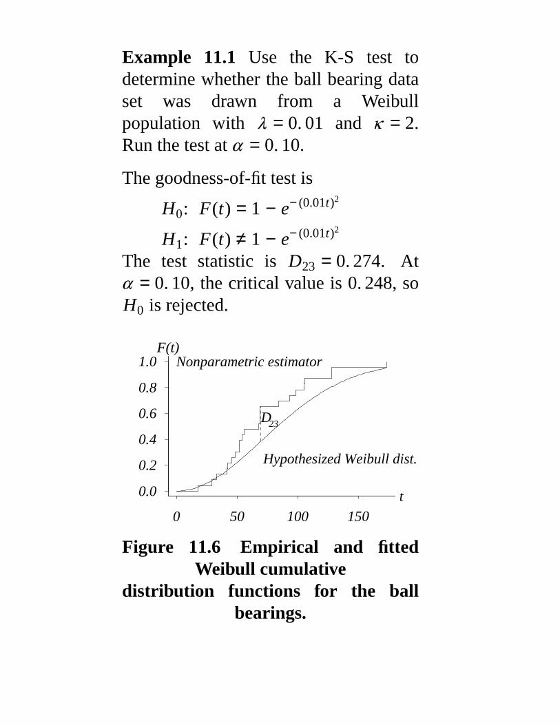
Example 11.1 Use the K-S test todetermine whether the ball bearing dataset was drawn from a Weibullpopulation with λ = 0. 01 and κ = 2.Run the test at α = 0. 10.
The goodness-of-fit test is
H0: F(t) = 1 − e− (0.01t)2
H1: F(t) ≠ 1 − e− (0.01t)2
The test statistic is D23 = 0. 274. Atα = 0. 10, the critical value is 0. 248, soH0 is rejected.
0 50 100 150
0.0
0.2
0.4
0.6
0.8
1.0
D23
Hypothesized Weibull dist.
Nonparametric estimator
t
F(t)
Figure 11.6 Empirical and fittedWeibull cumulative
distribution functions for the ballbearings.