Problem Decomposition and Task Mapping

CS 5334/4390 Spring 2014 Shirley Moore, Instructor

February 13 Class

1

Agenda

•  Announcements (5 min) •  Vote on attending Richard Tapia talk (5 min) •  Review of Gaussian Elimination and LU Decomposition (15 min) •  Problem Decomposition and Task Mapping (45 min) •  Wrapup and Homework (5 min)

2

Announcements

•  Deadline for registering for TACC Optimizing Code for Xeon Phi is tomorrow, Feb 14. Webcast is Friday, Feb 21.

•  Deadline for applying for XSEDE Summer Research Experiences has been extended to Saturday, Feb 22.

•  Richard Tapia talk next Tuesday, Feb 18, 3-4pm, conflicts with class. Vote on 1) do module on Pthreads programming outside of class and attend talk, vs 2) have class as usual.

3

Learning Objectives

•  After completing this week’s lessons, you should be able to –  Describe and use different problem decomposition techniques

–  Construct and analyze a task-dependency graph for a given problem decomposition

–  Construct and analyze an interaction graph for a given problem decomposition

–  Characterize inter-task interactions for a given problem

–  Describe and use block and block cyclic data distributions for array data

–  Compare and contrast static and dynamic task mapping

–  Describe methods for reducing task interaction overhead

4

Decomposition Techniques

So how does one decompose a task into various subtasks?

While no single recipe works for all problems, a set of commonly used techniques can be applied to broad classes of problems. These techniques include:

• recursive decomposition • data decomposition • exploratory decomposition • speculative decomposition

5

Recursive Decomposition

•  Generally suited to problems that are solved using a divide-and-conquer strategy.

•  The given problem is first decomposed into a set of sub-problems.

•  These sub-problems are recursively decomposed further until a desired granularity is reached.

6

Recursive Decomposition Example: Quicksort

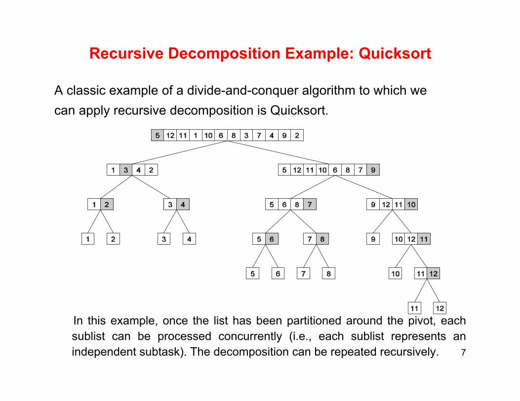
A classic example of a divide-and-conquer algorithm to which we can apply recursive decomposition is Quicksort.

In this example, once the list has been partitioned around the pivot, each sublist can be processed concurrently (i.e., each sublist represents an independent subtask). The decomposition can be repeated recursively.

11121096587342111121342348651311472912101168795121068758756101211119121012

7

Data Decomposition

•  Identify the data on which computations are performed. •  Partition the data across various tasks. •  The partitioning induces a decomposition of the problem into tasks

using the owner-computes rule. •  Data can be partitioned in various ways

–  Can critically impact performance of a parallel algorithm

8

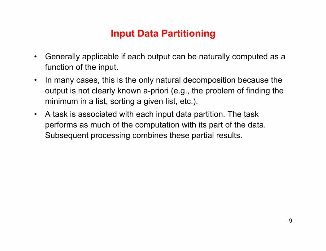
Input Data Partitioning

•  Generally applicable if each output can be naturally computed as a function of the input.

•  In many cases, this is the only natural decomposition because the output is not clearly known a-priori (e.g., the problem of finding the minimum in a list, sorting a given list, etc.).

•  A task is associated with each input data partition. The task performs as much of the computation with its part of the data. Subsequent processing combines these partial results.

9

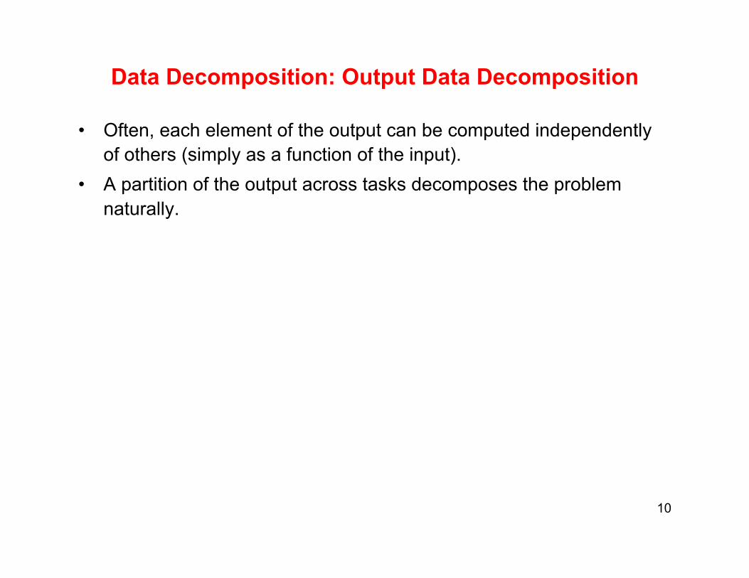
Data Decomposition: Output Data Decomposition

•  Often, each element of the output can be computed independently of others (simply as a function of the input).

•  A partition of the output across tasks decomposes the problem naturally.

10

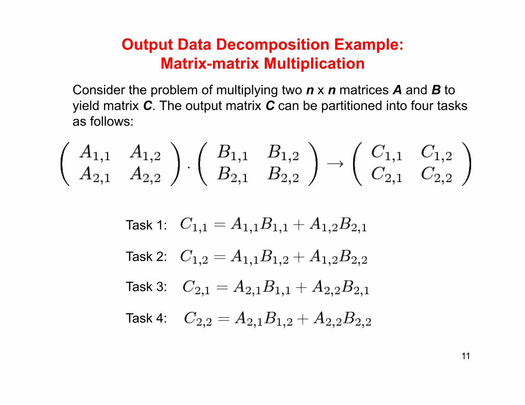
Output Data Decomposition Example: Matrix-matrix Multiplication

Consider the problem of multiplying two n x n matrices A and B to yield matrix C. The output matrix C can be partitioned into four tasks as follows:

Task 1:

Task 2:

Task 3:

Task 4:

11

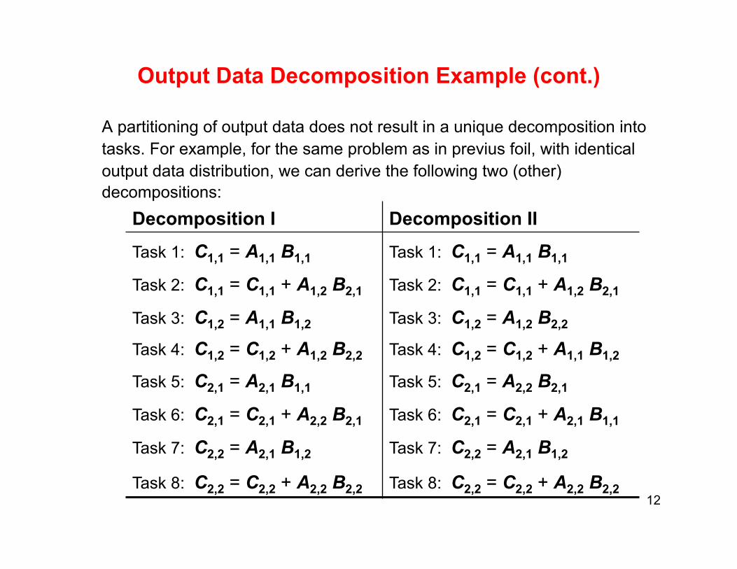
Output Data Decomposition Example (cont.)

A partitioning of output data does not result in a unique decomposition into tasks. For example, for the same problem as in previus foil, with identical output data distribution, we can derive the following two (other) decompositions:

Decomposition I Decomposition II

Task 1: C1,1 = A1,1 B1,1

Task 2: C1,1 = C1,1 + A1,2 B2,1

Task 3: C1,2 = A1,1 B1,2

Task 4: C1,2 = C1,2 + A1,2 B2,2

Task 5: C2,1 = A2,1 B1,1

Task 6: C2,1 = C2,1 + A2,2 B2,1

Task 7: C2,2 = A2,1 B1,2

Task 8: C2,2 = C2,2 + A2,2 B2,2

Task 1: C1,1 = A1,1 B1,1

Task 2: C1,1 = C1,1 + A1,2 B2,1

Task 3: C1,2 = A1,2 B2,2

Task 4: C1,2 = C1,2 + A1,1 B1,2

Task 5: C2,1 = A2,2 B2,1

Task 6: C2,1 = C2,1 + A2,1 B1,1

Task 7: C2,2 = A2,1 B1,2

Task 8: C2,2 = C2,2 + A2,2 B2,2 12

Intermediate Data Partitioning

•  Computation can often be viewed as a sequence of transformations from the input to the output data.

•  In such cases, it may be beneficial to use one of the intermediate stages as a basis for decomposition.

13

Intermediate Data Partitioning Example

Let us revisit the example of dense matrix multiplication. We first show how we can visualize this computation in terms of intermediate matrices D.

1,11,2BB1,1CDDDDDDDD1,1,1A2,11,1A2,2A1,2AB2,22,1B..+2,1,11,1,21,2,11,2,22,1,22,2,1CCC1,22,12,22,2,2

14

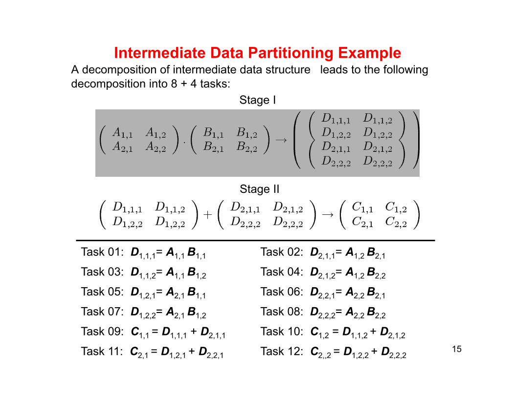
Intermediate Data Partitioning Example A decomposition of intermediate data structure leads to the following decomposition into 8 + 4 tasks:

Stage I

Stage II

Task 01: D1,1,1= A1,1 B1,1 Task 02: D2,1,1= A1,2 B2,1

Task 03: D1,1,2= A1,1 B1,2 Task 04: D2,1,2= A1,2 B2,2

Task 05: D1,2,1= A2,1 B1,1 Task 06: D2,2,1= A2,2 B2,1

Task 07: D1,2,2= A2,1 B1,2 Task 08: D2,2,2= A2,2 B2,2

Task 09: C1,1 = D1,1,1 + D2,1,1 Task 10: C1,2 = D1,1,2 + D2,1,2

Task 11: C2,1 = D1,2,1 + D2,2,1 Task 12: C2,,2 = D1,2,2 + D2,2,2 15

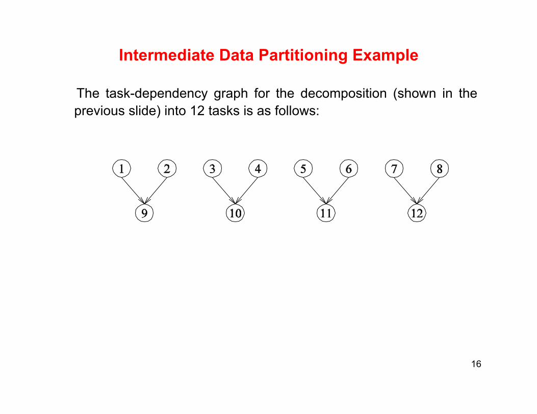
Intermediate Data Partitioning Example

The task-dependency graph for the decomposition (shown in the previous slide) into 12 tasks is as follows:

112342567891011

16

Exploratory Decomposition

•  In some cases, the decomposition of the problem goes hand-in-hand with its execution.

•  Such problems typically involve the exploration (search) of a state space of solutions.

•  Problems in this class include a variety of discrete optimization problems (0/1 integer programming, quadratic assignment, etc.), theorem proving, game playing, etc.

17

Exploratory Decomposition Example

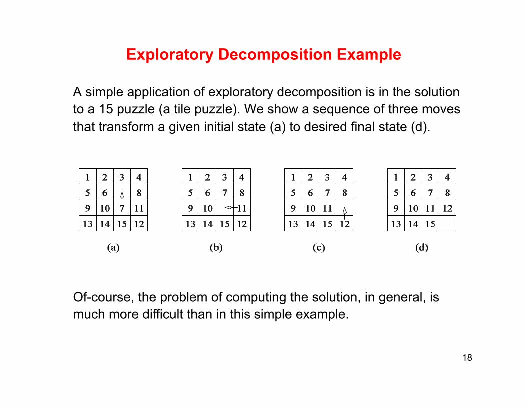
A simple application of exploratory decomposition is in the solution to a 15 puzzle (a tile puzzle). We show a sequence of three moves that transform a given initial state (a) to desired final state (d).

123456891013141512117123456789101314151211(d)123456789101113141512123456789101112131415(a)(b)(c)

Of-course, the problem of computing the solution, in general, is much more difficult than in this simple example.

18

Exploratory Decomposition: Example

The state space can be explored by generating various successor states of the current state and then viewing them as independent tasks. 1234567891013141512111234568910131415121171245689101314151211731234589101314151211761234569101314151211781234568910131415121171234567891314151211101234567813141512111091234578913141512111061234567891315121110task 114123456789131415121110123456789101312111514123456789101314121115123456789101314111512123456789101314121115123456789101314151211123456791013141512118123456789101314151211task 3task 2task 4123456789101314151112

19

Exploratory Decomposition: Anomalous Computations

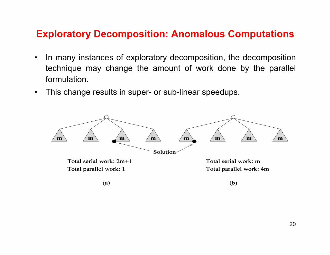
•  In many instances of exploratory decomposition, the decomposition technique may change the amount of work done by the parallel formulation.

•  This change results in super- or sub-linear speedups.

Solution(b)mmmmmmmmTotal serial work: 2m+1Total parallel work: 1Total serial work: mTotal parallel work: 4m(a)

20

Speculative Decomposition

•  In some applications, dependencies between tasks are not known a-priori.

•  For such applications, it is impossible to identify independent tasks. •  There are generally two approaches to dealing with such

applications: conservative approaches, which identify independent tasks only when they are guaranteed to not have dependencies, and, optimistic approaches, which schedule tasks even when they may potentially be erroneous.

•  Conservative approaches may yield little concurrency and optimistic approaches may require a roll-back mechanism in the case of an error.

21

Speculative Decomposition Example 1

A classic example of speculative decomposition is in discrete event simulation.

•  The central data structure in a discrete event simulation is a time-ordered event list.

•  Events are extracted precisely in time order, processed, and if required, resulting events are inserted back into the event list.

•  Consider your day today as a discrete event system - you get up, get ready, drive to school, go to class, eat lunch, go to another class, drive back, eat dinner, study, and sleep.

•  Each of these events can be processed independently assuming they will occur; however, in driving to school, you might meet with an unfortunate accident and not get to school at all.

•  Therefore, an optimistic scheduling of other events might have to be rolled back.

22

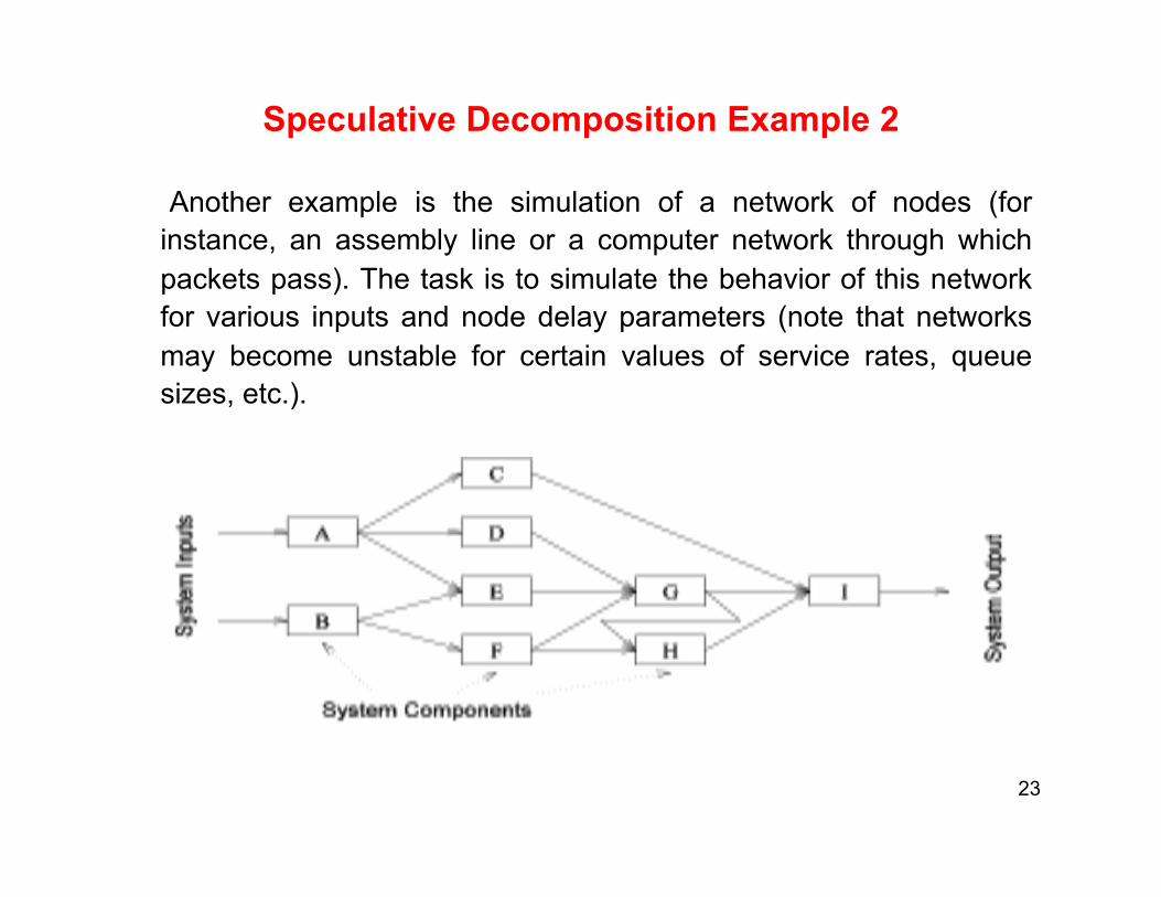
Speculative Decomposition Example 2

Another example is the simulation of a network of nodes (for instance, an assembly line or a computer network through which packets pass). The task is to simulate the behavior of this network for various inputs and node delay parameters (note that networks may become unstable for certain values of service rates, queue sizes, etc.).

23

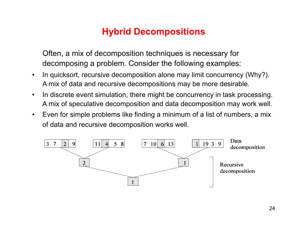
Hybrid Decompositions

2111RecursivedecompositionDatadecomposition3721175810613193994

Often, a mix of decomposition techniques is necessary for decomposing a problem. Consider the following examples:

•  In quicksort, recursive decomposition alone may limit concurrency (Why?). A mix of data and recursive decompositions may be more desirable.

•  In discrete event simulation, there might be concurrency in task processing. A mix of speculative decomposition and data decomposition may work well.

•  Even for simple problems like finding a minimum of a list of numbers, a mix of data and recursive decomposition works well.

24

Limits on Parallel Performance

•  It would appear that the parallel time can be made arbitrarily small by making the decomposition finer in granularity.

•  There is an inherent bound on how fine the granularity of a computation can be. For example, in the case of multiplying a dense matrix with a vector, there can be no more than (n2) concurrent tasks.

•  Concurrent tasks may also have to exchange data with other tasks. This results in communication overhead. The tradeoff between the granularity of a decomposition and associated overheads often determines performance bounds.

25

Task Interaction Graphs: An Example

Consider the problem of multiplying a sparse matrix A with a vector b. The following observations can be made:

45678910110b21A3(b)24613511109087Task 0Task 1184(a)

•  As before, the computation of each element of the result vector can be viewed as an independent task.

•  Unlike a dense matrix-vector product though, only non-zero elements of matrix A participate in the computation.

•  If, for memory optimality, we also partition b across tasks, then one can see that the task interaction graph of the computation is identical to the graph of the matrix A (the graph for which A represents the adjacency structure).

26

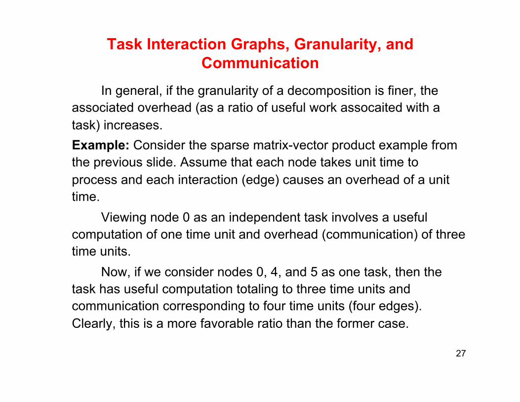
Task Interaction Graphs, Granularity, and Communication

In general, if the granularity of a decomposition is finer, the associated overhead (as a ratio of useful work assocaited with a task) increases. Example: Consider the sparse matrix-vector product example from the previous slide. Assume that each node takes unit time to process and each interaction (edge) causes an overhead of a unit time. Viewing node 0 as an independent task involves a useful computation of one time unit and overhead (communication) of three time units. Now, if we consider nodes 0, 4, and 5 as one task, then the task has useful computation totaling to three time units and communication corresponding to four time units (four edges). Clearly, this is a more favorable ratio than the former case.

27

Processes and Mapping

•  In general, the number of tasks in a decomposition may exceed the number of processing elements available, or the opposite may be true.

•  A parallel algorithm must also provide a mapping of tasks to processes.

Note: We refer to the mapping as being from tasks to processes, as opposed to processors. This is because typical programming APIs, as we shall see, do not allow easy binding of tasks to physical processors (although this situation is improving). Rather, we aggregate tasks into processes and rely on the system to map these processes to physical processors (although we may be able to give “hints”). We use processes, not in the UNIX sense of a process, rather, simply as a collection of tasks and associated data.

28

Processes and Mapping

•  Appropriate mapping of tasks to processes is critical to the parallel performance of an algorithm.

•  Mappings are determined by both the task dependency and task interaction graphs.

•  Task dependency graphs can be used to ensure that work is equally spread across all processes at any point (minimum idling and optimal load balance).

•  Task interaction graphs can be used to make sure that processes need minimum interaction with other processes (minimum communication).

29

Processes and Mapping

An appropriate mapping must minimize parallel execution time by:

•  Mapping independent tasks to different processes.

•  Assigning tasks on critical path to processes as soon as they become available.

•  Minimizing interaction between processes by mapping tasks with dense interactions to the same process.

Note: These criteria often conflict eith each other. For example, a decomposition into one task (or no decomposition at all) minimizes interaction but does not result in a speedup at all! Can you think of other such conflicting cases?

30

Characteristics of Tasks

Once a problem has been decomposed into independent tasks, the characteristics of these tasks critically impact choice and performance of mappings. Relevant task characteristics include:

•  Task generation •  Task sizes •  Size of data associated with tasks

31

Task Generation

•  Static task generation –  Concurrent tasks can be identified a-priori.

–  Typical matrix operations, graph algorithms, image processing applications, and other regularly structured problems fall in this class.

–  These can typically be decomposed using data or recursive decomposition techniques.

•  Dynamic task generation –  Tasks are generated as we perform computation. A classic example of

this is in game playing - each 15 puzzle board is generated from the previous one.

–  These applications are typically decomposed using exploratory or speculative decompositions.

32

Task Sizes

•  Task sizes may be uniform (i.e., all tasks are the same size) or non-uniform.

•  Non-uniform task sizes may be such that they can be determined (or estimated) a-priori or not. –  Examples in the latter class include discrete optimization problems, in

which it is difficult to estimate the effective size of a state space.

33

Size of Data Associated with Tasks

•  The size of data associated with a task may be small or large when viewed in the context of the size of the task.

•  A small context of a task implies that an algorithm can easily communicate this task to other processes dynamically (e.g., the 15 puzzle).

•  A large context ties the task to a process, or alternately, an algorithm may attempt to reconstruct the context at another processes as opposed to communicating the context of the task (e.g., 0/1 integer programming).

34

Characteristics of Task Interactions

•  Static interactions –  The tasks and their interactions are known a-priori.

–  These are relatively simpler to code into programs.

•  Dynamic interactions –  The interactions between tasks cannot be determined a-priori.

–  These interactions are harder to code, especially when using message passing APIs.

•  Regular interactions –  There is a definite pattern (in the graph sense) to the interactions.

–  These patterns can be exploited for efficient implementation.

•  Irregular interactions –  Interactions lack well-defined topologies.

35

Characteristics of Task Interactions: Example

PixelsTasks

A simple example of a regular static interaction pattern is in image dithering. The underlying communication pattern is between neighbors in a structured 2-D mesh as shown below.

36

Characteristics of Task Interactions: Example

45678910110b21A3(b)24613511109087Task 0Task 1184(a)

The multiplication of a sparse matrix with a vector is a good example of a static irregular interaction pattern. Here is an example of a sparse matrix and its associated interaction pattern.

37

Characteristics of Task Interactions (cont.)

•  Interactions may be read-only or read-write. –  In read-only interactions, tasks just read data items associated with

other tasks.

–  In read-write interactions tasks read as well as modify data items associated with other tasks.

–  In general, read-write interactions are harder to code, since they require additional synchronization primitives.

38

Characteristics of Task Interactions (cont.)

•  Interactions may be one-way or two-way. –  A one-way interaction can be initiated and accomplished by one of the

two interacting tasks.

–  A two-way interaction requires participation from both tasks involved in an interaction.

–  One way interactions are somewhat harder to code in message passing APIs.

39

Mapping Techniques

•  Once a problem has been decomposed into concurrent tasks, these must be mapped to processes (that can be executed on a parallel platform).

•  Mappings shoud try to minimize overheads. •  Primary overheads are communication and idling. •  Minimizing these overheads often presents contradicting objectives. •  Assigning all work to one processor trivially minimizes

communication at the expense of significant idling.

40

Mapping Techniques for Minimum Idling

121110P19P2synchronizationP3P4t = 0start1t = 0start12345678finisht = 323456789101112synchronizationt = 3finisht = 6(a)(b)P1P2P3P4t = 2

Mapping must simultaneously minimize idling and load balance. Merely balancing load does not minimize idling.

41

Mapping Techniques for Minimum Idling

Mapping techniques can be static or dynamic.

•  Static Mapping: Tasks are mapped to processes a-priori. For this to work, we must have a good estimate of the size of each task. Even in these cases, the problem may be NP complete.

•  Dynamic Mapping: Tasks are mapped to processes at runtime. This may be because the tasks are generated at runtime, or that their sizes are not known.

Other factors that determine the choice of techniques include the size of data associated with a task and the nature of underlying domain.

42

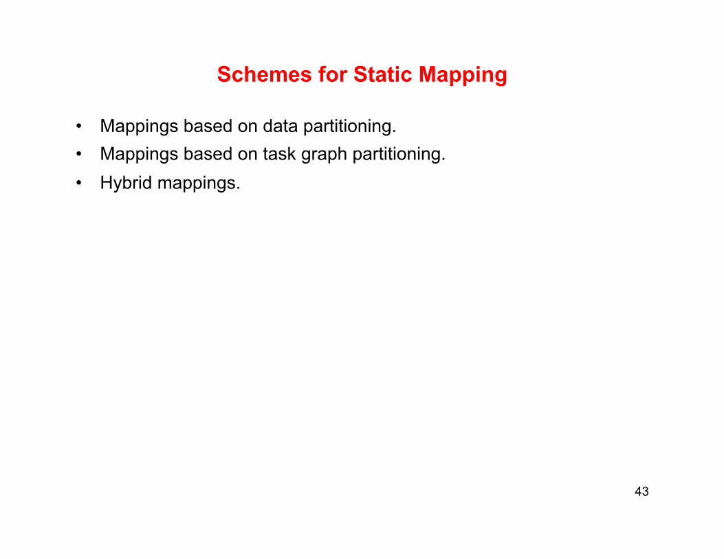
Schemes for Static Mapping

•  Mappings based on data partitioning. •  Mappings based on task graph partitioning. •  Hybrid mappings.

43

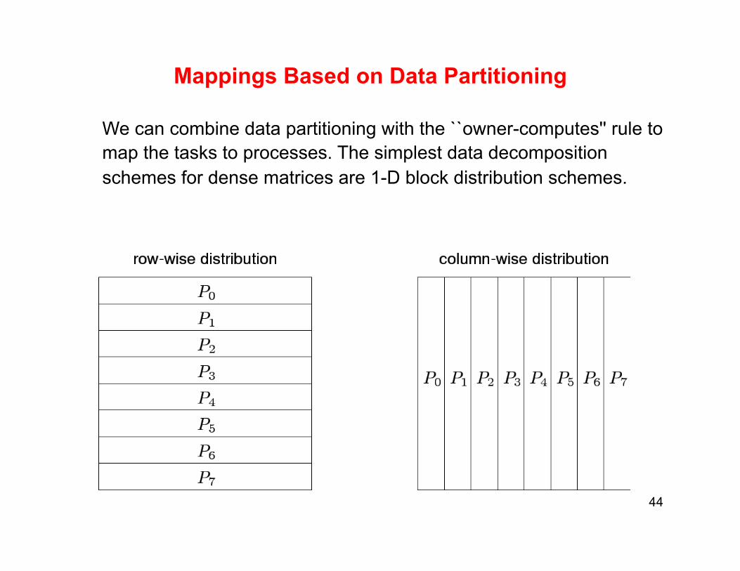
Mappings Based on Data Partitioning

We can combine data partitioning with the ``owner-computes'' rule to map the tasks to processes. The simplest data decomposition schemes for dense matrices are 1-D block distribution schemes.

44

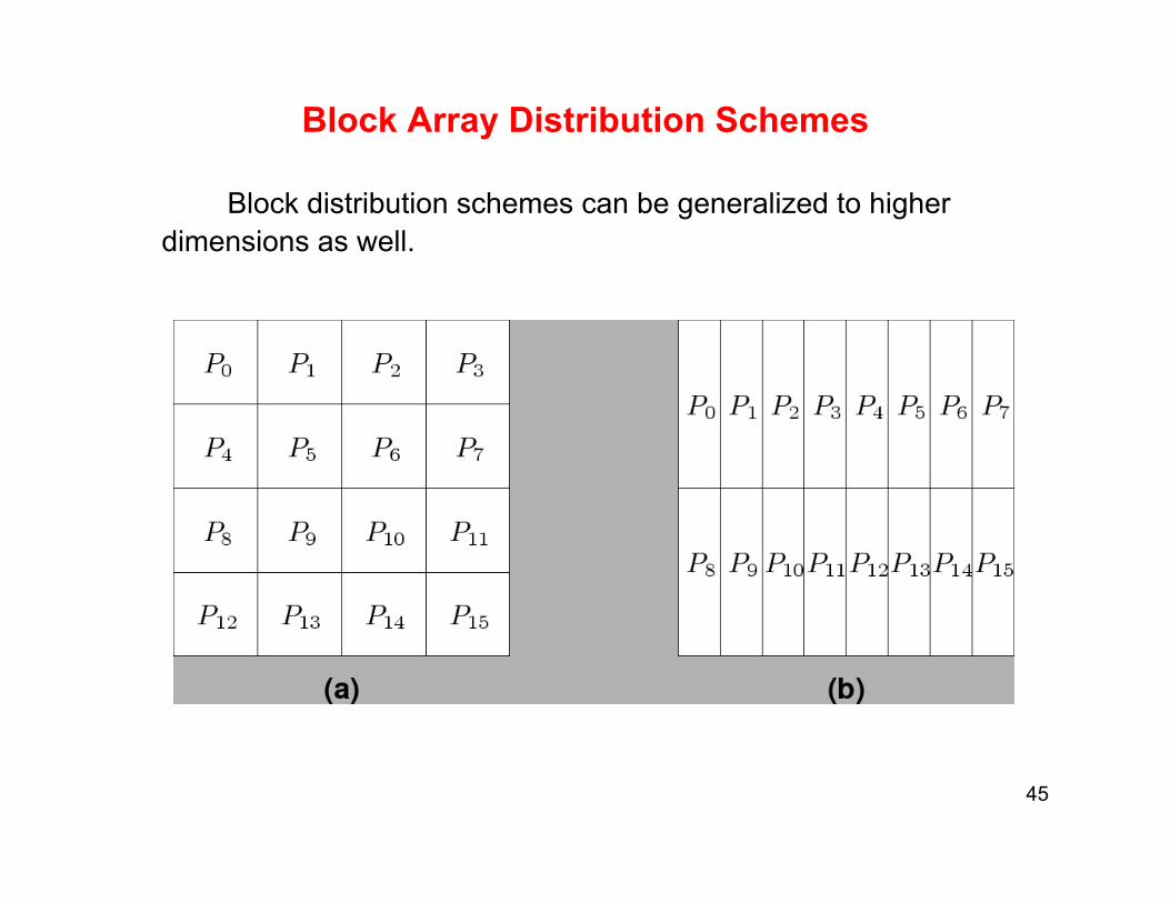
Block Array Distribution Schemes

Block distribution schemes can be generalized to higher dimensions as well.

45

Block Array Distribution Schemes: Examples

•  For multiplying two dense matrices A and B, we can partition the output matrix C using a block decomposition.

•  For load balance, we give each task the same number of elements of C. (Note that each element of C corresponds to a single dot product.)

•  The choice of decomposition (1-D or 2-D) is determined by the associated communication overhead.

•  In general, higher dimension decomposition reduces communication and allows the use of a larger number of processes.

46

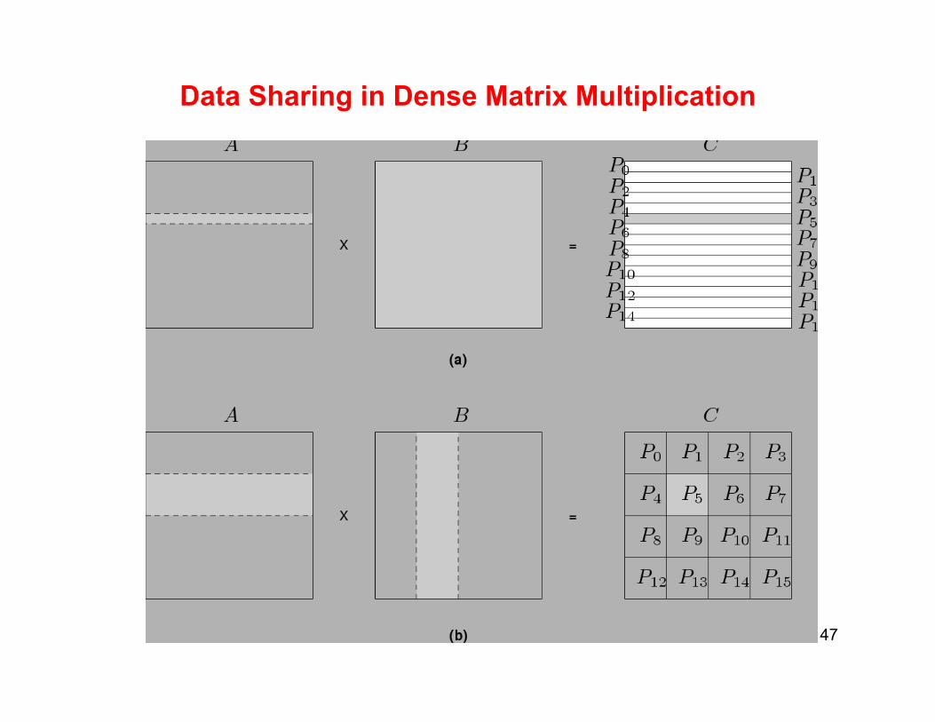
Data Sharing in Dense Matrix Multiplication

47

Cyclic and Block Cyclic Distributions

•  If the amount of computation associated with data items varies, a block decomposition may lead to significant load imbalances.

•  An example of this is LU decomposition of dense matrices.

48

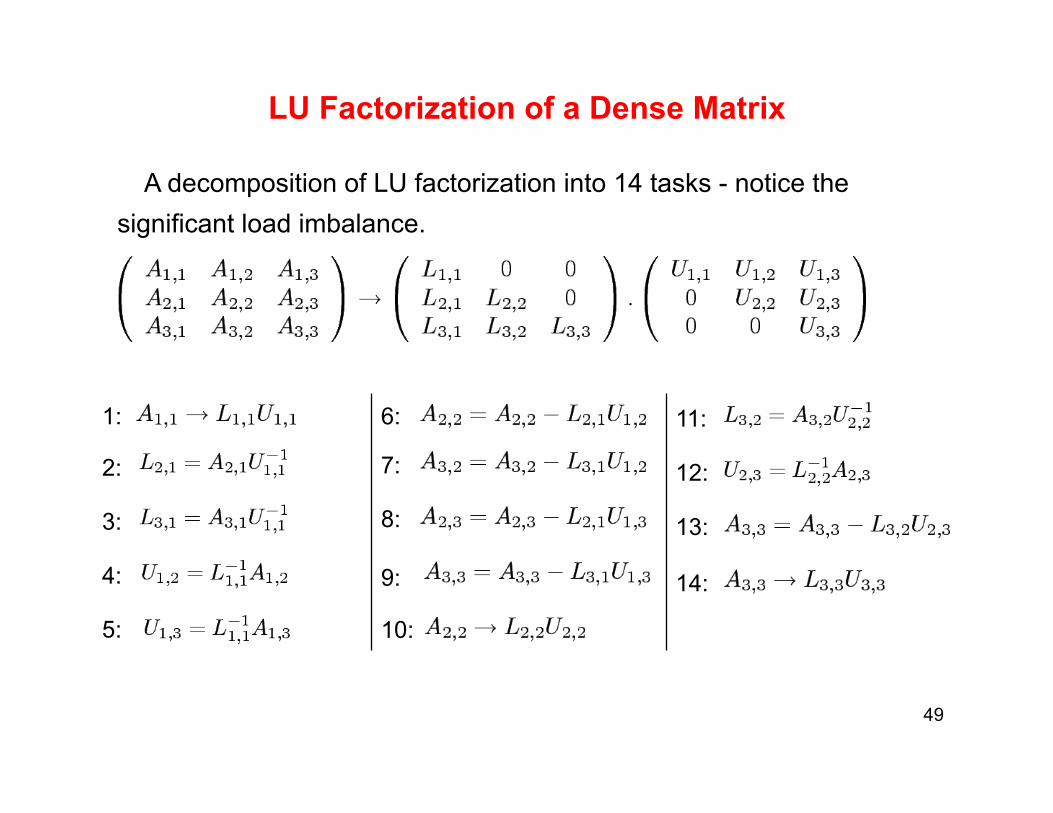
LU Factorization of a Dense Matrix

A decomposition of LU factorization into 14 tasks - notice the significant load imbalance.

1:

2:

3:

4:

5:

6:

7:

8:

9:

10:

11:

12:

13:

14:

49

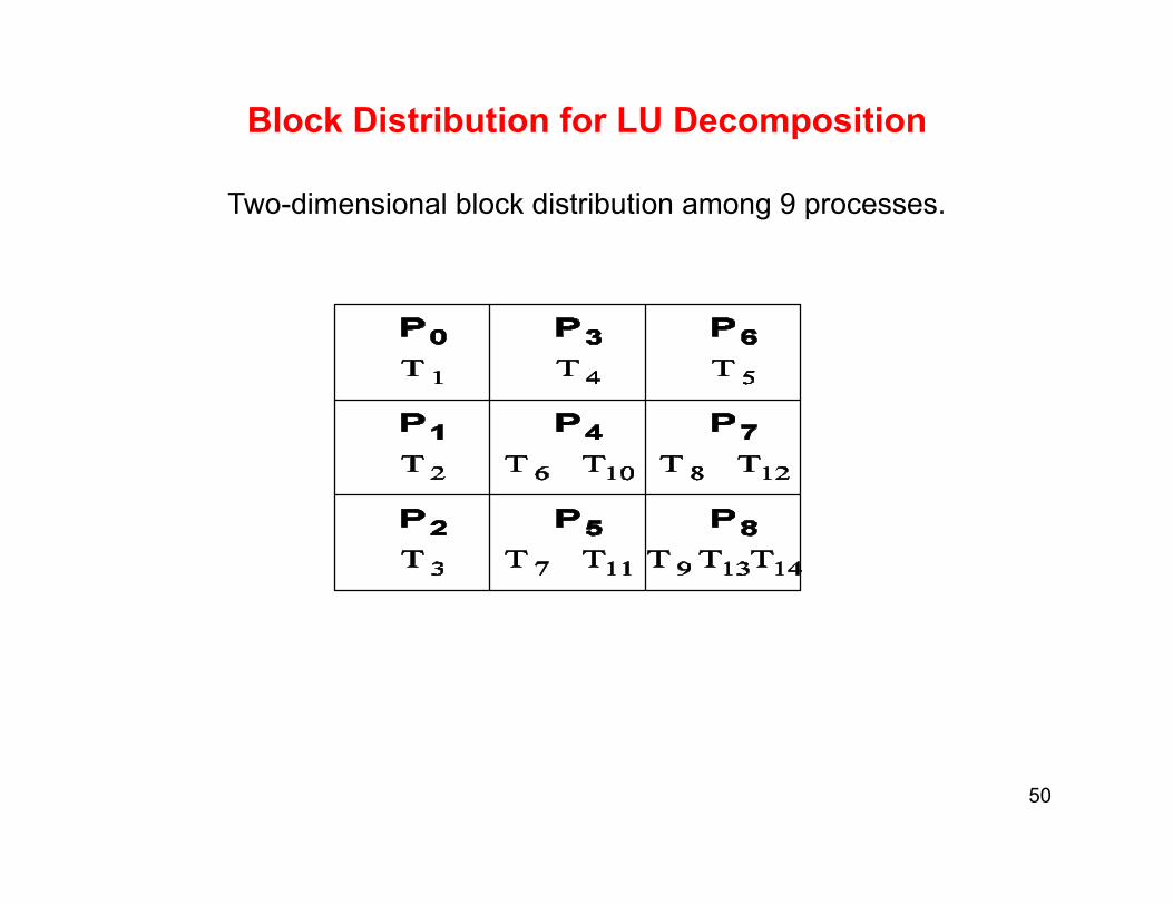
Block Distribution for LU Decomposition

0PPPPP1PTTPTTTPTTTTPT14TTTT623457812345610789111213

Two-dimensional block distribution among 9 processes.

50

Block Cyclic Distribution

•  Variation of the block distribution scheme that can be used to alleviate the load-imbalance and idling problems.

•  Partition an array into many more blocks than the number of available processes.

•  Blocks are assigned to processes in a round-robin manner so that each process gets several non-adjacent blocks.

51

Block-Cyclic Distribution for LU Decomposition

A[i,j] := A[i,j] - A[i,k] A[k,jRow kRow i(k,k)(k,j)Inactive partActive partA[k,j] := A[k,j]/A[k,k]x(i,k)(i,j)Column kColumn j

The active part of the matrix in LU decompositin changes. By assigning blocks in a block-cyclic fashion, each processor receives blocks from different parts of the matrix.

52

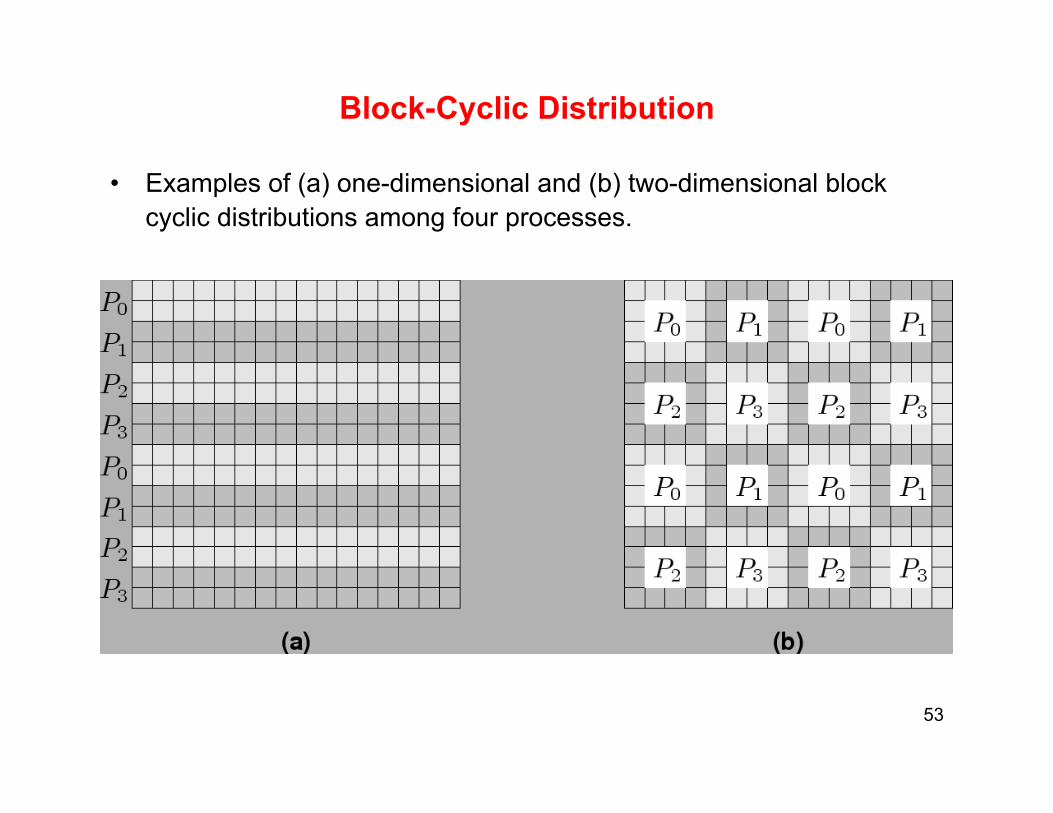
Block-Cyclic Distribution

•  Examples of (a) one-dimensional and (b) two-dimensional block cyclic distributions among four processes.

53

Graph Partitioning Based Data Decomposition

•  In case of sparse matrices, block decompositions are more complex. –  Consider the problem of multiplying a sparse matrix with a vector.

–  The graph of the matrix is a useful indicator of the work (number of nodes) and communication (the degree of each node).

–  In this case, we would like to partition the graph so as to assign equal number of nodes to each process, while minimizing the edge count of the graph partition.

•  Another example of a graph-based problem is simulation of a physical phenomenon that uses a mesh – e.g., fluid dynamics, fractures, deformable objects

54

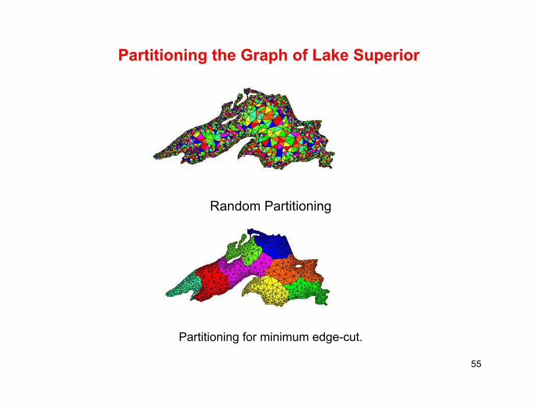
Partitioning the Graph of Lake Superior

Random Partitioning

Partitioning for minimum edge-cut.

55

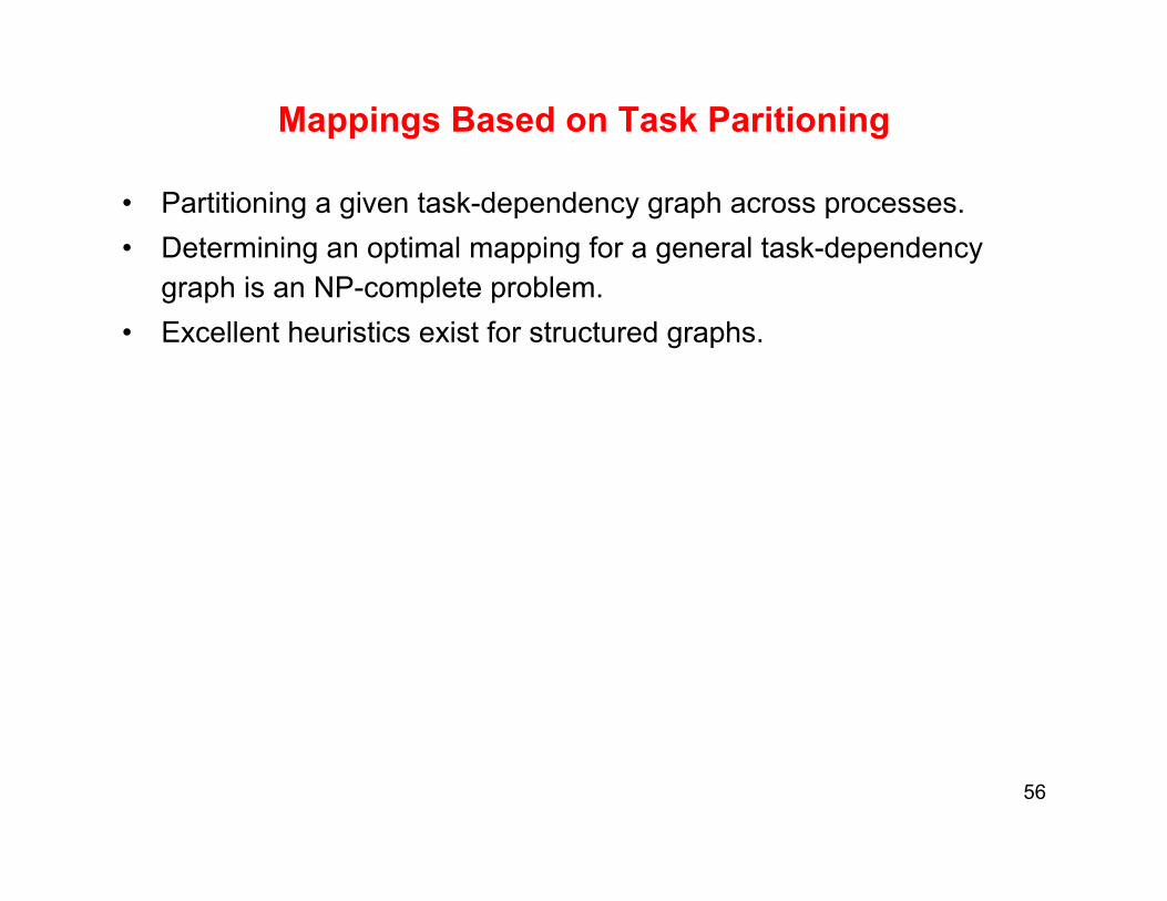
Mappings Based on Task Paritioning

•  Partitioning a given task-dependency graph across processes. •  Determining an optimal mapping for a general task-dependency

graph is an NP-complete problem. •  Excellent heuristics exist for structured graphs.

56

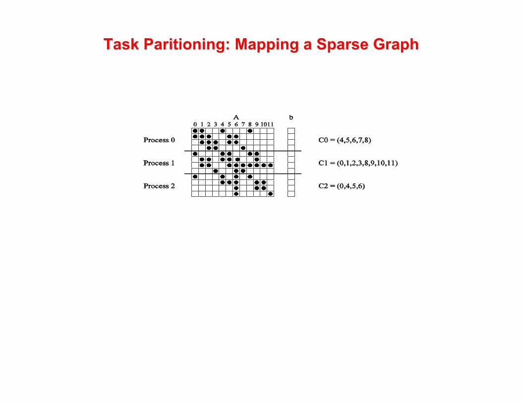
Task Paritioning: Mapping a Sparse Graph

45678910110C2 = (0,4,5,6)21bC1 = (0,1,2,3,8,9,10,11)C0 = (4,5,6,7,8)3Process 0Process 1Process 2A

C2 = (1,2,4,5,7,8)24613511109087C1 = (0,5,6)Process 1Process 0Process 2C0 = (1,2,6,9)

Sparse graph for computing a sparse matrix-vector product and its mapping.

57

Schemes for Dynamic Mapping

•  Dynamic mapping is sometimes also referred to as dynamic load balancing, since load balancing is the primary motivation for dynamic mapping.

•  Dynamic mapping schemes can be centralized or distributed.

58

Centralized Dynamic Mapping

•  Processes are designated as masters or slaves. •  When a process runs out of work, it requests the master for more

work. •  When the number of processes increases, the master may become

the bottleneck. •  To alleviate this, a process may pick up a number of tasks (a chunk)

at one time. This is called Chunk scheduling. •  Selecting large chunk sizes may lead to significant load imbalances

as well. •  A number of schemes have been devised to gradually decrease

chunk size as the computation progresses.

59

Distributed Dynamic Mapping

•  Each process can send or receive work from other processes. •  This alleviates the bottleneck in centralized schemes. •  There are four critical questions: how are sensing and receiving

processes paired together, who initiates work transfer, how much work is transferred, and when is a transfer triggered?

•  Answers to these questions are generally application specific. We will look at some of these techniques later in this class.

60

Minimizing Interaction Overheads

•  Maximize data locality: Where possible, reuse intermediate data. Restructure computation so that data can be reused in smaller time windows.

•  Minimize volume of data exchange: There is a cost associated with each word that is communicated. For this reason, we must minimize the volume of data communicated.

•  Minimize frequency of interactions: There is a startup cost associated with each interaction. Therefore, try to merge multiple interactions to one, where possible.

•  Minimize contention and hot-spots: Use decentralized techniques, replicate data where necessary.

61

Minimizing Interaction Overheads (continued)

•  Overlapping computations with interactions: Use non-blocking communications, multithreading, and prefetching to hide latencies.

•  Replicating data or computations. •  Using group communications instead of point-to-point primitives. •  Overlap interactions with other interactions.

62

Homework

•  Homework 2 due Tuesday, Feb 25 –  Chapter 3 problems 3.5, 3.6, 3.7, 3.8, 3.9, 3.19, 3.20

•  Reading for Tuesday, Feb 18: Chapter 7, pp. 279-311.

63