Problem Set #5-Key

Sonoma State University Dr. Cuellar

Economics 317- Introduction to Econometrics

Using Dummy Variables

Using data the data set CPS-Econ317, answer the following questions. Note, this is a

large data set and you may need to increase the amount of ram allocated to STATA.

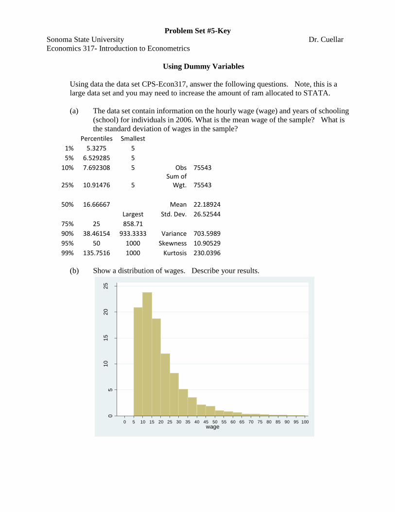
(a) The data set contain information on the hourly wage (wage) and years of schooling

(school) for individuals in 2006. What is the mean wage of the sample? What is

the standard deviation of wages in the sample?

Percentiles Smallest

1% 5.3275 5 5% 6.529285 5 10% 7.692308 5 Obs 75543

25% 10.91476 5 Sum of

Wgt. 75543

50% 16.66667

Mean 22.18924

Largest Std. Dev. 26.52544

75% 25 858.71 90% 38.46154 933.3333 Variance 703.5989

95% 50 1000 Skewness 10.90529

99% 135.7516 1000 Kurtosis 230.0396

(b) Show a distribution of wages. Describe your results.

05

10

15

20

25

Pe

rcen

t

0 5 10 15 20 25 30 35 40 45 50 55 60 65 70 75 80 85 90 95 100

wage

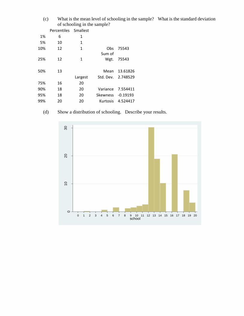
(c) What is the mean level of schooling in the sample? What is the standard deviation

of schooling in the sample?

Percentiles Smallest

1% 6 1 5% 10 1 10% 12 1 Obs 75543

25% 12 1 Sum of

Wgt. 75543

50% 13

Mean 13.61826

Largest Std. Dev. 2.748529

75% 16 20 90% 18 20 Variance 7.554411

95% 18 20 Skewness -0.19193

99% 20 20 Kurtosis 4.524417

(d) Show a distribution of schooling. Describe your results.

01

02

03

0

Pe

rcen

t

0 1 2 3 4 5 6 7 8 9 10 11 12 13 14 15 16 17 18 19 20

school

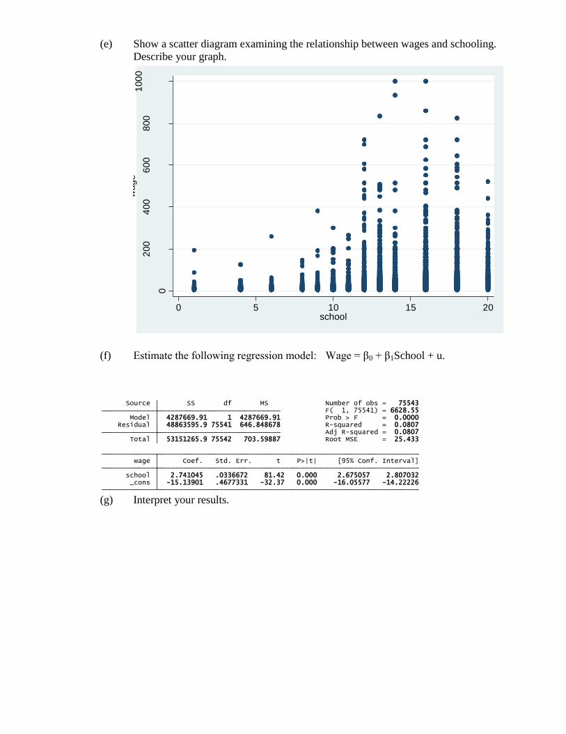
(e) Show a scatter diagram examining the relationship between wages and schooling.

Describe your graph.

(f) Estimate the following regression model: Wage = β0 + β1School + u.

(g) Interpret your results.

0

200

400

600

800

100

0w

ag

e

0 5 10 15 20school

_cons -15.13901 .4677331 -32.37 0.000 -16.05577 -14.22226 school 2.741045 .0336672 81.42 0.000 2.675057 2.807032 wage Coef. Std. Err. t P>|t| [95% Conf. Interval]

Total 53151265.9 75542 703.59887 Root MSE = 25.433 Adj R-squared = 0.0807 Residual 48863595.9 75541 646.848678 R-squared = 0.0807 Model 4287669.91 1 4287669.91 Prob > F = 0.0000 F( 1, 75541) = 6628.55 Source SS df MS Number of obs = 75543

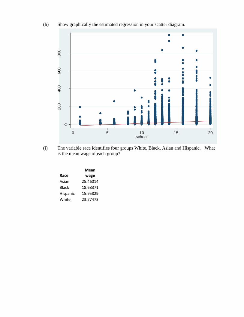
(h) Show graphically the estimated regression in your scatter diagram.

(i) The variable race identifies four groups White, Black, Asian and Hispanic. What

is the mean wage of each group?

Race Mean wage

Asian 25.46014

Black 18.68371

Hispanic 15.95829

White 23.77473

0

200

400

600

800

100

0

0 5 10 15 20school

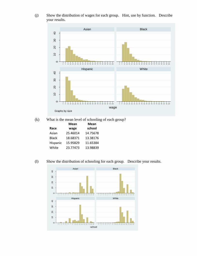
(j) Show the distribution of wages for each group. Hint, use by function. Describe

your results.

(k) What is the mean level of schooling of each group?

Race Mean wage

Mean school

Asian 25.46014 14.75678

Black 18.68371 13.38176

Hispanic 15.95829 11.65384

White 23.77473 13.98839

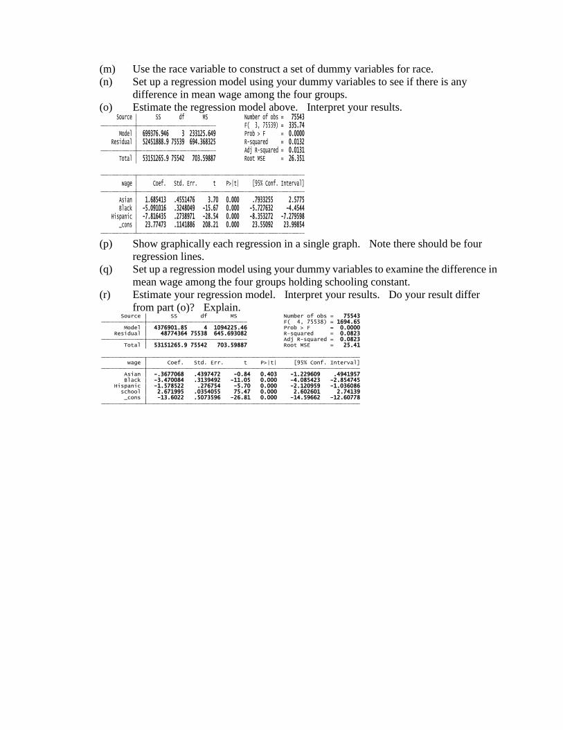
(l) Show the distribution of schooling for each group. Describe your results.

01

02

03

04

00

10

20

30

40

0 5 10 15 20 25 30 35 40 45 50 55 60 65 70 75 80 85 90 95 100 0 5 10 15 20 25 30 35 40 45 50 55 60 65 70 75 80 85 90 95 100

0 5 10 15 20 25 30 35 40 45 50 55 60 65 70 75 80 85 90 95 100 0 5 10 15 20 25 30 35 40 45 50 55 60 65 70 75 80 85 90 95 100

Asian Black

Hispanic White

Pe

rcen

t

wageGraphs by race

01

02

03

04

00

10

20

30

40

0 1 2 3 4 5 6 7 8 9 10 11 12 13 14 15 16 17 18 19 20 0 1 2 3 4 5 6 7 8 9 10 11 12 13 14 15 16 17 18 19 20

0 1 2 3 4 5 6 7 8 9 10 11 12 13 14 15 16 17 18 19 20 0 1 2 3 4 5 6 7 8 9 10 11 12 13 14 15 16 17 18 19 20

Asian Black

Hispanic White

Pe

rcen

t

school

(m) Use the race variable to construct a set of dummy variables for race.

(n) Set up a regression model using your dummy variables to see if there is any

difference in mean wage among the four groups.

(o) Estimate the regression model above. Interpret your results.

(p) Show graphically each regression in a single graph. Note there should be four

regression lines.

(q) Set up a regression model using your dummy variables to examine the difference in

mean wage among the four groups holding schooling constant.

(r) Estimate your regression model. Interpret your results. Do your result differ

from part (o)? Explain.

_cons 23.77473 .1141886 208.21 0.000 23.55092 23.99854 Hispanic -7.816435 .2738971 -28.54 0.000 -8.353272 -7.279598 Black -5.091016 .3248049 -15.67 0.000 -5.727632 -4.4544 Asian 1.685413 .4551476 3.70 0.000 .7933255 2.5775 wage Coef. Std. Err. t P>|t| [95% Conf. Interval]

Total 53151265.9 75542 703.59887 Root MSE = 26.351 Adj R-squared = 0.0131 Residual 52451888.9 75539 694.368325 R-squared = 0.0132 Model 699376.946 3 233125.649 Prob > F = 0.0000 F( 3, 75539) = 335.74 Source SS df MS Number of obs = 75543

_cons -13.6022 .5073596 -26.81 0.000 -14.59662 -12.60778 school 2.671995 .0354055 75.47 0.000 2.602601 2.74139 Hispanic -1.578522 .276754 -5.70 0.000 -2.120959 -1.036086 Black -3.470084 .3139492 -11.05 0.000 -4.085423 -2.854745 Asian -.3677068 .4397472 -0.84 0.403 -1.229609 .4941957 wage Coef. Std. Err. t P>|t| [95% Conf. Interval]

Total 53151265.9 75542 703.59887 Root MSE = 25.41 Adj R-squared = 0.0823 Residual 48774364 75538 645.693082 R-squared = 0.0823 Model 4376901.85 4 1094225.46 Prob > F = 0.0000 F( 4, 75538) = 1694.65 Source SS df MS Number of obs = 75543

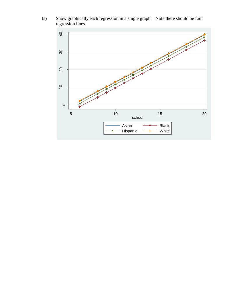
(s) Show graphically each regression in a single graph. Note there should be four

regression lines.

01

02

03

04

0

5 10 15 20school

Asian Black

Hispanic White