Problem Solving and Search in Artificial Intelligence

Algorithm Selection

Nysret MusliuDatabase and Artificial Intelligence GroupInstitut of Logic and Computation, TU Wien

2

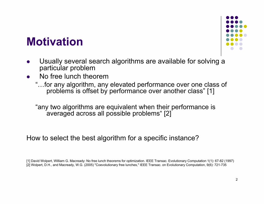
Motivation Usually several search algorithms are available for solving a

particular problem No free lunch theorem

“…for any algorithm, any elevated performance over one class of problems is offset by performance over another class” [1]

“any two algorithms are equivalent when their performance is averaged across all possible problems“ [2]

How to select the best algorithm for a specific instance?

[1] David Wolpert, William G. Macready: No free lunch theorems for optimization. IEEE Transac. Evolutionary Computation 1(1): 67-82 (1997)[2] Wolpert, D.H., and Macready, W.G. (2005) "Coevolutionary free lunches," IEEE Transac. on Evolutionary Computation, 9(6): 721-735

3

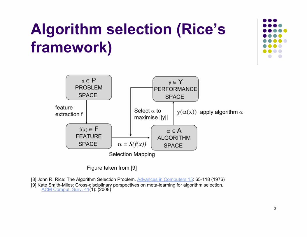
Algorithm selection (Rice’s framework)

Figure taken from [9]

[8] John R. Rice: The Algorithm Selection Problem. Advances in Computers 15: 65-118 (1976) [9] Kate Smith-Miles: Cross-disciplinary perspectives on meta-learning for algorithm selection.

ACM Comput. Surv. 41(1): (2008)

4

Algorithm selectionInput (see [8] and [9]): Problem space P that represents the set of instances of a problem class A feature space F that contains measurable characteristics of the

instances generated by a computational feature extraction process applied to P

Set A of all considered algorithms for tackling the problem The performance space Y represents the mapping of each algorithm to

a set of performance metrics

Problem:For a given problem instance x E P, with features f(x) E F, find the

selection mapping S(f(x)) into algorithm space , such that the selected algorithm a E A maximizes the performance mapping y(a(x)) E Y

[8] John R. Rice: The Algorithm Selection Problem. Advances in Computers 15: 65-118 (1976) [9] Kate Smith-Miles: Cross-disciplinary perspectives on meta-learning for algorithm selection. ACM Comput. Surv. 41(1): (2008)

5

Algorithm selection An important issue is the selection of appropriate features

Example: Selection of sorting algorithms based on features ([10]):

Degree of pre-sortedness of the starting sequence Length of sequence

A supervised machine learning approach can be used to select the algorithm to be used based on features of the input instance

A training set with instances (and their features) and best performing algorithm should be provided to the supervised machine learning algorithms to train them

[9] Kate Smith-Miles: Cross-disciplinary perspectives on meta-learning for algorithm selection. ACM Comput. Surv. 41(1): (2008) [10] Guo, H. 2003. Algorithm selection for sorting and probabilistic inference: A machine learning-based approach.Ph.D. dissertation, Kansas State University.

6

Algorithm selection for sorting [10] P=43195 instances of random sequences of different sizes and

complexities A=5 sorting algorithms (InsertionSort, ShellSort, heapSort,

mergeSort, QuickSort) Y=algorithm rank based on CPU time to achieve sorted

sequence F=3 measures of presortedness and length of sequences (size) Machine learning methods: C4.5, Naïve Bayes, Bayesian

network learner

Different other examples are given in [9] [10] Guo, H. 2003. Algorithm selection for sorting and probabilistic inference: A machine learning-based approach.Ph.D. dissertation, Kansas State University.

7

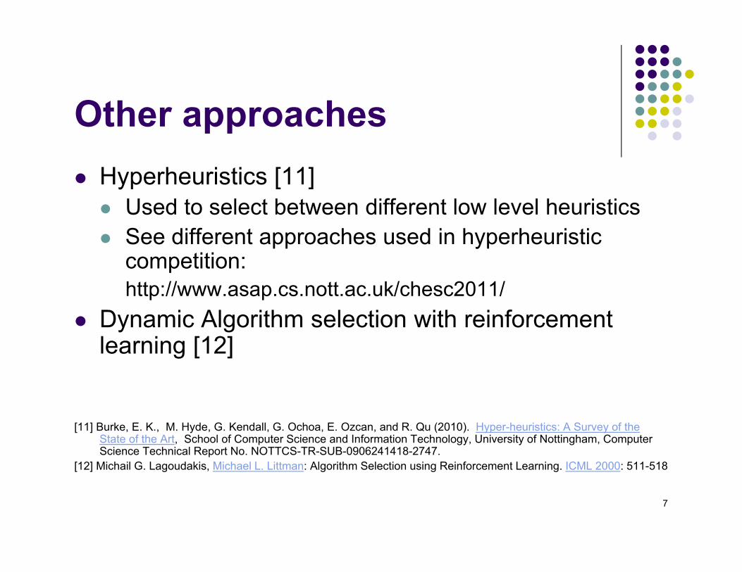
Other approaches Hyperheuristics [11] Used to select between different low level heuristics See different approaches used in hyperheuristic

competition:http://www.asap.cs.nott.ac.uk/chesc2011/

Dynamic Algorithm selection with reinforcement learning [12]

[11] Burke, E. K., M. Hyde, G. Kendall, G. Ochoa, E. Ozcan, and R. Qu (2010). Hyper-heuristics: A Survey of the State of the Art, School of Computer Science and Information Technology, University of Nottingham, Computer Science Technical Report No. NOTTCS-TR-SUB-0906241418-2747.

[12] Michail G. Lagoudakis, Michael L. Littman: Algorithm Selection using Reinforcement Learning. ICML 2000: 511-518

8

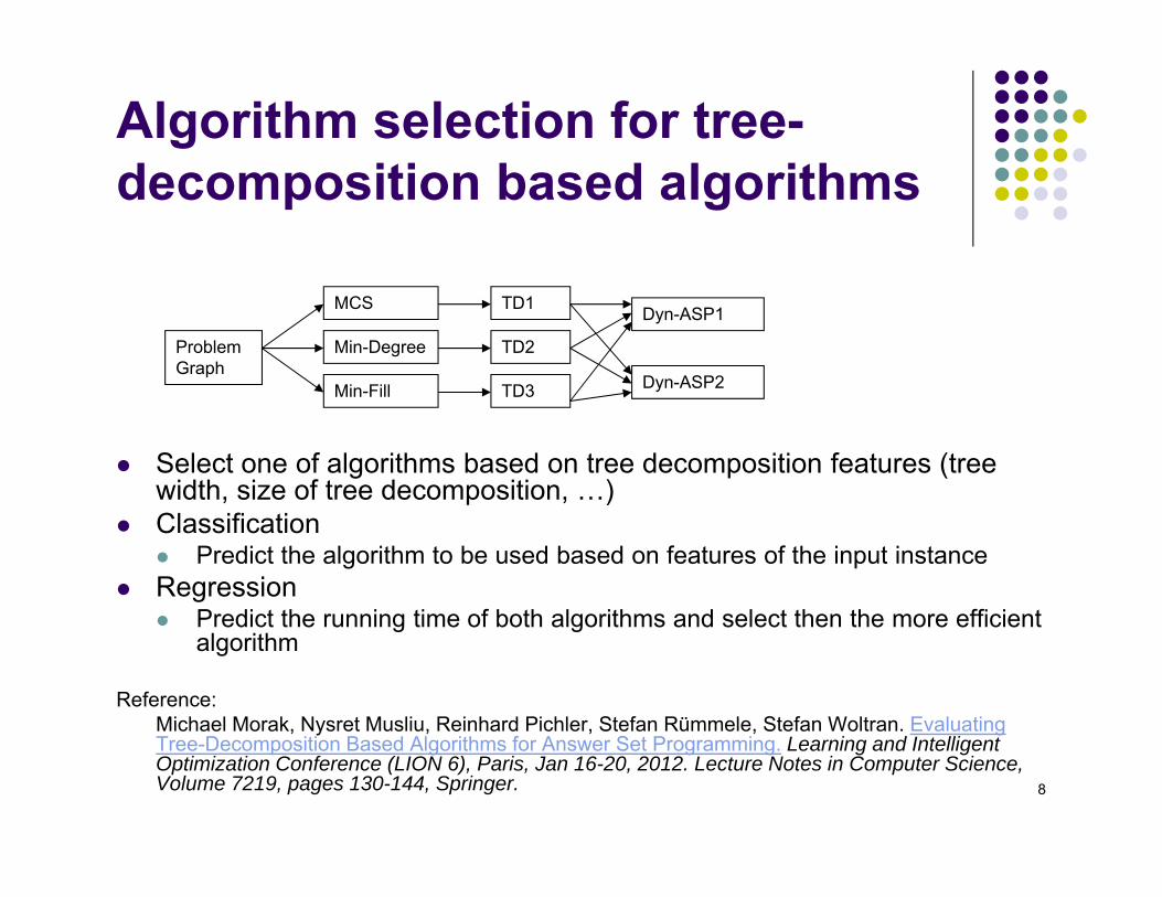
Algorithm selection for tree-decomposition based algorithms

Select one of algorithms based on tree decomposition features (tree width, size of tree decomposition, …)

Classification Predict the algorithm to be used based on features of the input instance

Regression Predict the running time of both algorithms and select then the more efficient

algorithm

Reference: Michael Morak, Nysret Musliu, Reinhard Pichler, Stefan Rümmele, Stefan Woltran. Evaluating Tree-Decomposition Based Algorithms for Answer Set Programming. Learning and Intelligent Optimization Conference (LION 6), Paris, Jan 16-20, 2012. Lecture Notes in Computer Science, Volume 7219, pages 130-144, Springer.

ProblemGraph

MCS

Min-Degree

Min-Fill

TD1

TD2

TD3

Dyn-ASP1

Dyn-ASP2

9

Case Studies Case study 1:

Application of Machine Learning for Algorithm Selection in Graph ColoringReferences:

Martin Schwengerer. Algorithm Selection for the Graph Coloring Problem. Master Thesis, Vienna University of Technology, 2012.

Nysret Musliu, Martin Schwengerer. Algorithm Selection for the Graph Coloring Problem.Learning and Intelligent OptimizatioN Conference (LION 7), Catania - Italy, Jan 7-11, 2013. Lecture Notes in Computer Science, to appear.

Case study 2: Improving the Efficiency of Dynamic Programming on Tree Decompositions via

Machine LearningReferences: Michael Abseher, Nysret Musliu, Stefan Woltran. Improving the Efficiency of Dynamic

Programming on Tree Decompositions via Machine Learning. J. Artif. Intell. Res. 58: 829-858 (2017)

Michael Abseher, Frederico Dusberger, Nysret Musliu, Stefan Woltran. Improving the Efficiency of Dynamic Programming on Tree Decompositions via Machine Learning. IJCAI 2015: 275-282

Algorithm Selection for the Graph ColoringProblem

Nysret Musliu Martin Schwengerer

DBAI Group, Institute of Information Systems, Vienna University of Technology

Learning and Intelligent OptimizatioN Conference 2013

Supported by FWF (The Austrian Science Fund) andFFG (The Austrian Research Promotion Agency).

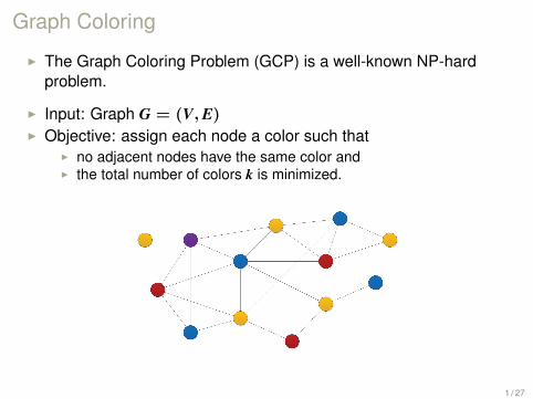
Graph Coloring

I The Graph Coloring Problem (GCP) is a well-known NP-hardproblem.

I Input: Graph G = (V,E)I Objective: assign each node a color such that

I no adjacent nodes have the same color andI the total number of colors k is minimized.

1 / 27

Graph Coloring (cont.)

I Exact approaches are in general only usable up to 100 nodes.

I Several (meta)heuristic approaches:I Tabu searchI Simulated annealingI Genetic algorithmI Ant colony optimizationI ...

I But: None of these techniques is superior to all others.

I Practical issue: Which heuristic should be used?

I Our approach: Select for each instance the algorithm which isexpected to give best performance.

2 / 27

Graph Coloring (cont.)

I Exact approaches are in general only usable up to 100 nodes.

I Several (meta)heuristic approaches:I Tabu searchI Simulated annealingI Genetic algorithmI Ant colony optimizationI ...

I But: None of these techniques is superior to all others.

I Practical issue: Which heuristic should be used?

I Our approach: Select for each instance the algorithm which isexpected to give best performance.

2 / 27

Algorithm Selection

I Algorithm Selection Problem by Rice [RICE, 1976]

I Main components:I Problem space PI Feature space FI Algorithm space AI Performance space Y

I Task: Find a selector S that selects for an instance i ∈ P the bestalgorithm a ∈ A.

3 / 27

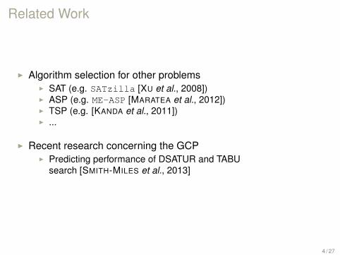
Related Work

I Algorithm selection for other problemsI SAT (e.g. SATzilla [XU et al., 2008])I ASP (e.g. ME-ASP [MARATEA et al., 2012])I TSP (e.g. [KANDA et al., 2011])I ...

I Recent research concerning the GCPI Predicting performance of DSATUR and TABU

search [SMITH-MILES et al., 2013]

4 / 27

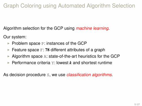
Graph Coloring using Automated Algorithm Selection

Algorithm selection for the GCP using machine learning.

Our system:I Problem space P: instances of the GCPI Feature space F: 78 different attributes of a graphI Algorithm space A: state-of-the-art heuristics for the GCPI Performance criteria Y: lowest k and shortest runtime

As decision procedure S, we use classification algorithms.

5 / 27

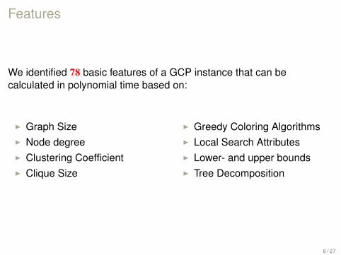
Features

We identified 78 basic features of a GCP instance that can becalculated in polynomial time based on:

I Graph SizeI Node degreeI Clustering CoefficientI Clique Size

I Greedy Coloring AlgorithmsI Local Search AttributesI Lower- and upper boundsI Tree Decomposition

6 / 27

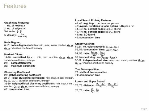
Features

Graph Size Features:1: no. of nodes: n2: no. of edges: m3,4: ratio: n

m , mn

5: density: 2·mn·(n−1)

Node Degree:6-13: nodes degree statistics: min, max, mean, median, Q0.25,Q0.75, variation coefficient, entropy

Maximal Clique:14-20: normalized by n: min, max, median, Q0.25, Q0.75,variation coefficient, entropy21: computation time22: maximum cardinality

Clustering Coefficient23: global clustering coefficient24-31: local clustering coefficient: min, max, mean, median,Q0.25, Q0.75, variation coefficient, entropy32-39: weighted local clustering coefficient: min, max, mean,median, Q0.25 , Q0.75 , variation coefficient, entropy40: computation time

Local Search Probing Features:41, 42: avg. impr.: per iteration, per run43: avg no. iterations to local optima (LO) per a run44, 45: no. conflict nodes: at LO, at end46, 47: no. conflict edges: at LO, at end48: no. LO found49: computation time

Greedy Coloring:50,51: no. colors needed: kDSAT , kRLF52, 53: computation time: tDSAT , tRLF

54, 55: ratio: kDSATkRLF

, kRLFkRLF

56: best coloring: min(kDSAT, kRLF)57-72: independent-set size: min, max, mean, median, Q0.25,Q0.75, variation coefficient, entropy

Tree Decomposition:73: width of decomposition74: computation time

Lower- and Upper Bound:

75, 76: distance: (Bl−Bu)Bl

, (Bu−Bl)Bu

77, 78: ratio: BlBu

, BuBl

7 / 27

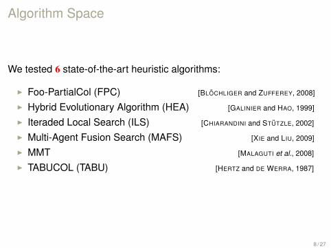
Algorithm Space

We tested 6 state-of-the-art heuristic algorithms:

I Foo-PartialCol (FPC) [BLOCHLIGER and ZUFFEREY, 2008]

I Hybrid Evolutionary Algorithm (HEA) [GALINIER and HAO, 1999]

I Iteraded Local Search (ILS) [CHIARANDINI and STUTZLE, 2002]

I Multi-Agent Fusion Search (MAFS) [XIE and LIU, 2009]

I MMT [MALAGUTI et al., 2008]

I TABUCOL (TABU) [HERTZ and DE WERRA, 1987]

8 / 27

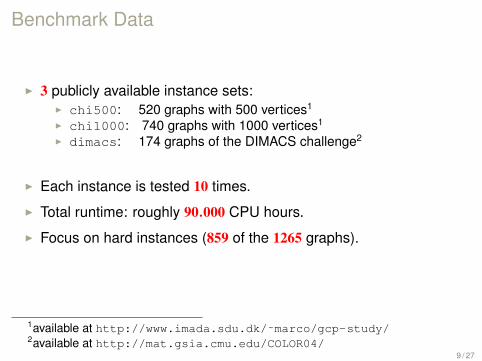
Benchmark Data

I 3 publicly available instance sets:I chi500: 520 graphs with 500 vertices1

I chi1000: 740 graphs with 1000 vertices1

I dimacs: 174 graphs of the DIMACS challenge2

I Each instance is tested 10 times.

I Total runtime: roughly 90.000 CPU hours.

I Focus on hard instances (859 of the 1265 graphs).

1available at http://www.imada.sdu.dk/˜marco/gcp-study/2available at http://mat.gsia.cmu.edu/COLOR04/

9 / 27

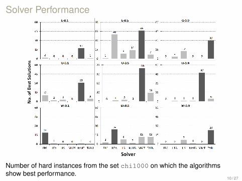
Solver Performance

Number of hard instances from the set chi1000 on which the algorithmsshow best performance.

10 / 27

Selection Procedure

I We tested 6 popular classification algorithms:I Bayesian Networks (BN)I C4.5 Decision Trees (DT)I k-Nearest Neighbor (kNN)I Random Forests (RF)I Multilayer Perceptrons (MLP)I Support-Vector Machines (SVM)

I with several parameter configurations for each classifier.

11 / 27

Other Important Issues

In addition, we experimented with:I Effect of Data Preparation:

I Study the effect of two discretization methods:I The classical minimum-descriptive length (MDL) andI Kononenko’s criteria (KON).

I Feature Selection:I Use best-first and a genetic search strategy to identify useful

features.

12 / 27

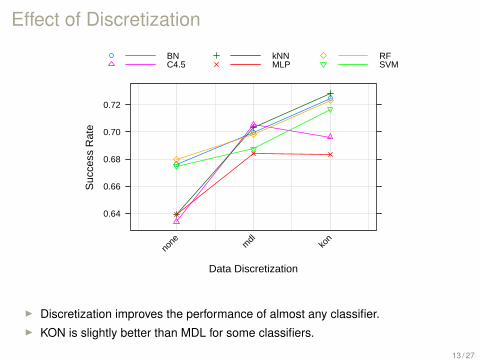
Effect of Discretization

Data Discretization

Suc

cess

Rat

e

0.64

0.66

0.68

0.70

0.72

none m

dlko

n

BNC4.5

kNNMLP

RFSVM

I Discretization improves the performance of almost any classifier.I KON is slightly better than MDL for some classifiers.

13 / 27

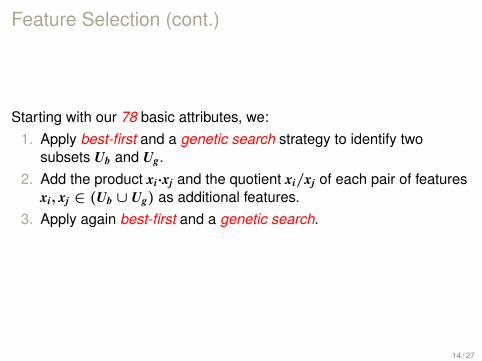
Feature Selection (cont.)

Starting with our 78 basic attributes, we:1. Apply best-first and a genetic search strategy to identify two

subsets Ub and Ug.2. Add the product xi·xj and the quotient xi/xj of each pair of features

xi, xj ∈ (Ub ∪ Ug) as additional features.3. Apply again best-first and a genetic search.

14 / 27

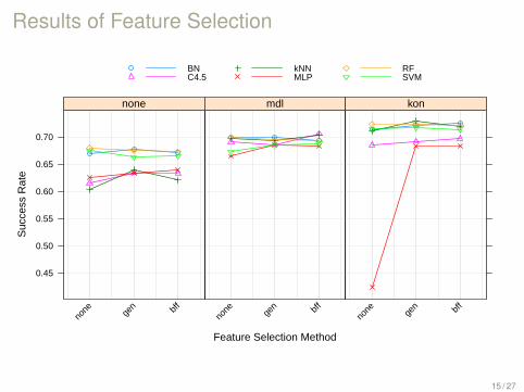
Results of Feature Selection

Feature Selection Method

Suc

cess

Rat

e

0.45

0.50

0.55

0.60

0.65

0.70

none ge

n bff

none

none ge

n bff

mdl

none ge

n bff

kon

BNC4.5

kNNMLP

RFSVM

15 / 27

Results of Feature Selection and Data Discretization

I Use the feature subset obtained by the genetic search.I Data discretized with Kononenko’s criteria.

16 / 27

Results on the Training Data

Results of 20 runs of a 10-fold cross-validation using KON and the results ofthe genetic search.

17 / 27

Results on the Training Data (cont.)

I We further applied a corrected resampled T-test with α = 0.05using cross-validation.

Results:I BN, kNN and RF are significant better than DT.I All other pairwise comparisons do not show significant differences.

18 / 27

Evaluation on the Test Set

I We create a test set with 180 graphs of different class, size anddensity.

I Our system based on automated algorithm selection:I Using the all 6 heuristics.I Trained with the benchmark data.I Data discretized with Kononenko’s criteria.

19 / 27

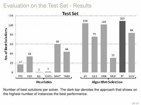
Evaluation on the Test Set - Results

Number of best solutions per solver. The dark bar denotes the approach that shows onthe highest number of instances the best performance.

20 / 27

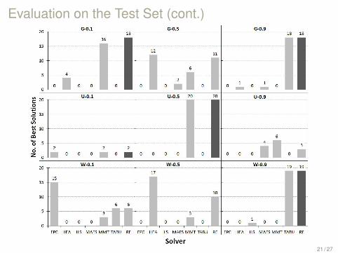
Evaluation on the Test Set (cont.)

21 / 27

Conclusion

I We applied automated algorithm selection for the GCP.I Key features:

I 78 basic features of an GCP instance.I 6 state-of-the-art heuristics.I Training data of 859 hard graphs.I Classification algorithms as selection procedure.

Results:I Classification algorithms predicts for up to 70.39% of the graphs the

most suited algorithm.I Improvement of +33.55% compared with the best solver.

22 / 27

References II BLOCHLIGER, I. and ZUFFEREY, N. (2008).

Computers & Operations Research 35, 960–975.

I CHIARANDINI, M. and STUTZLE, T. (2002).An application of Iterated Local Search to Graph Coloring.In JOHNSON, D. S., MEHROTRA, A., and TRICK, M. A., editors, Proceedings of the Computational Symposium on GraphColoring and its Generalizations, pages 112–125, Ithaca, New York, USA.

I GALINIER, P. and HAO, J.-K. (1999).Journal of Combinatorial Optimization 3, 379–397.

I HERTZ, A. and DE WERRA, D. (1987).Computing 39, 345–351.

I KANDA, J., CARVALHO, A., HRUSCHKA, E., and SOARES, C. (2011).Neural Networks 8.

I MALAGUTI, E., MONACI, M., and TOTH, P. (2008).INFORMS Journal on Computing 20, 302–316.

I MARATEA, M., PULINA, L., and RICCA, F. (2012).Applying Machine Learning Techniques to ASP Solving.In DOVIER, A. and COSTA, V. S., editors, ICLP (Technical Communications), volume 17 of LIPIcs, pages 37–48. SchlossDagstuhl - Leibniz-Zentrum fuer Informatik.

I RICE, J. R. (1976).Advances in Computers 15, 65–118.

I SMITH-MILES, K., WREFORD, B., LOPES, L., and INSANI, N. (2013).Predicting Metaheuristic Performance on Graph Coloring Problems Using Data Mining.In Hybrid Metaheuristics, Studies in Computational Intelligence, pages 417–432.

I XIE, X.-F. and LIU, J. (2009).Journal of Combinatorial Optimization 18, 99–123.

25 / 27

References II

I XU, L., HUTTER, F., HOOS, H. H., and LEYTON-BROWN, K. (2008).Journal of Artificial Intelligence Research 32.

26 / 27

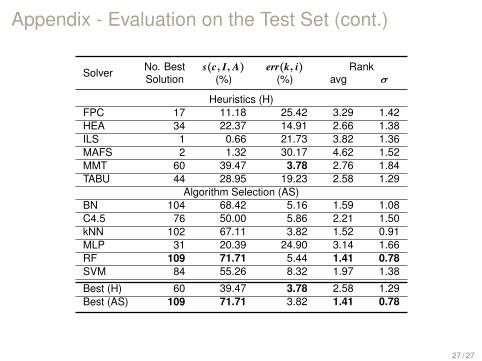
Appendix - Evaluation on the Test Set (cont.)

Solver No. Best s(c, I, A) err(k, i) RankSolution (%) (%) avg σ

Heuristics (H)FPC 17 11.18 25.42 3.29 1.42HEA 34 22.37 14.91 2.66 1.38ILS 1 0.66 21.73 3.82 1.36MAFS 2 1.32 30.17 4.62 1.52MMT 60 39.47 3.78 2.76 1.84TABU 44 28.95 19.23 2.58 1.29

Algorithm Selection (AS)BN 104 68.42 5.16 1.59 1.08C4.5 76 50.00 5.86 2.21 1.50kNN 102 67.11 3.82 1.52 0.91MLP 31 20.39 24.90 3.14 1.66RF 109 71.71 5.44 1.41 0.78SVM 84 55.26 8.32 1.97 1.38

Best (H) 60 39.47 3.78 2.58 1.29Best (AS) 109 71.71 3.82 1.41 0.78

27 / 27

Improving the Efficiency of Dynamic Programming on Tree Decompositions via Machine Learning

Michael Abseher, Frederico Dusberger, Nysret Musliu, Stefan WoltranTU Wien

The work is supported by the Austrian Science Fund

IJCAI 2015

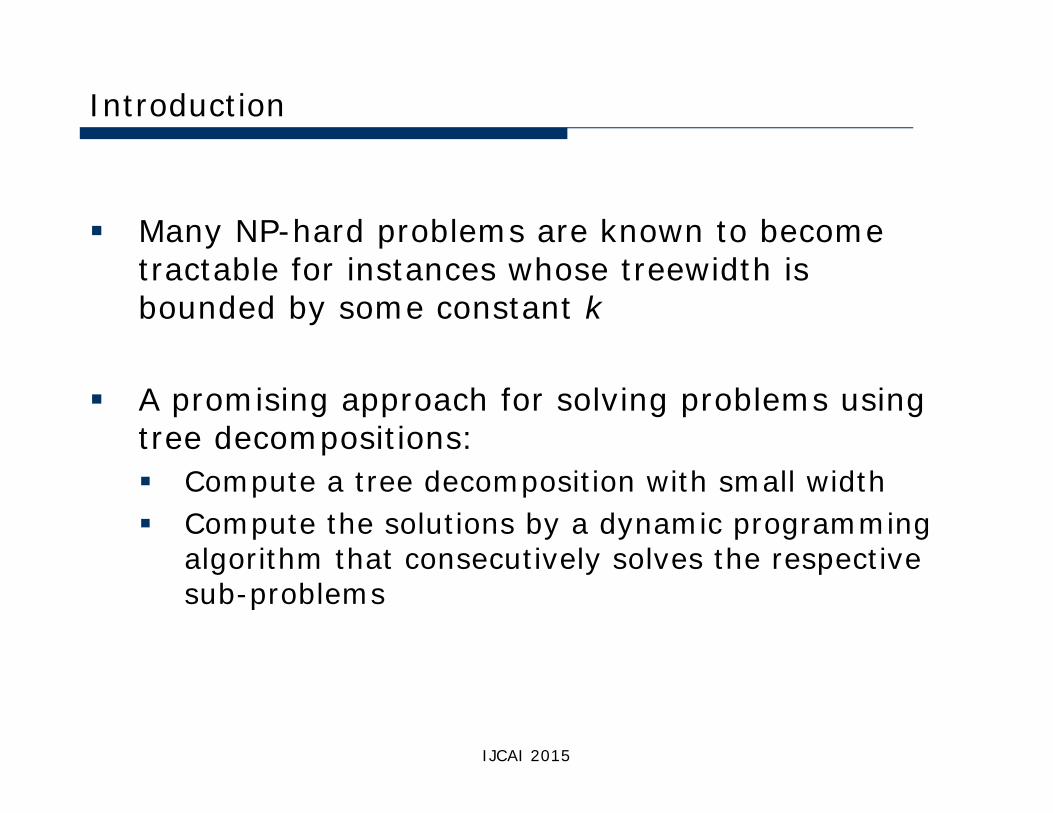
Introduction

Many NP-hard problems are known to become tractable for instances whose treewidth is bounded by some constant k

A promising approach for solving problems using tree decompositions: Compute a tree decomposition with small width Compute the solutions by a dynamic programming

algorithm that consecutively solves the respective sub-problems

IJCAI 2015

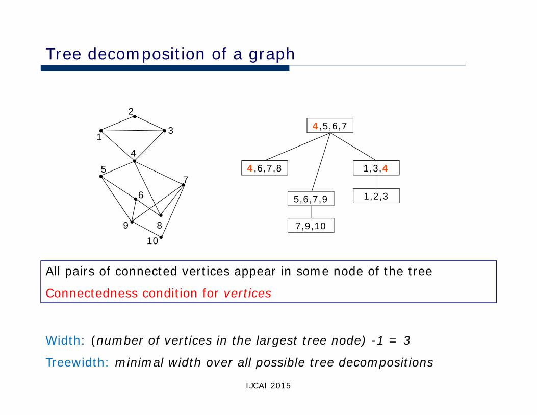
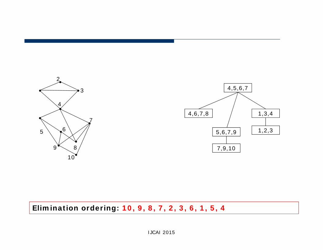
Tree decomposition of a graph

All pairs of connected vertices appear in some node of the tree

Connectedness condition for vertices

1

2

3

45

67

8910

7,9,10

5,6,7,9

4,6,7,8

4,5,6,7

1,2,3

1,3,4

Width: (number of vertices in the largest tree node) -1 = 3

Treewidth: minimal width over all possible tree decompositions

IJCAI 2015

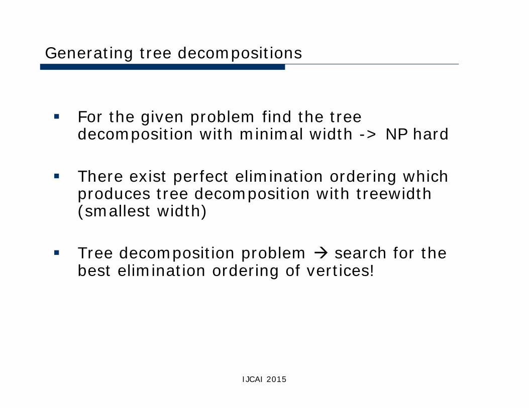
Generating tree decompositions

For the given problem find the tree decomposition with minimal width -> NP hard

There exist perfect elimination ordering which produces tree decomposition with treewidth(smallest width)

Tree decomposition problem search for the best elimination ordering of vertices!

IJCAI 2015

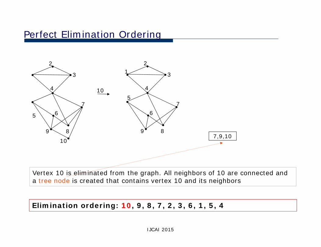
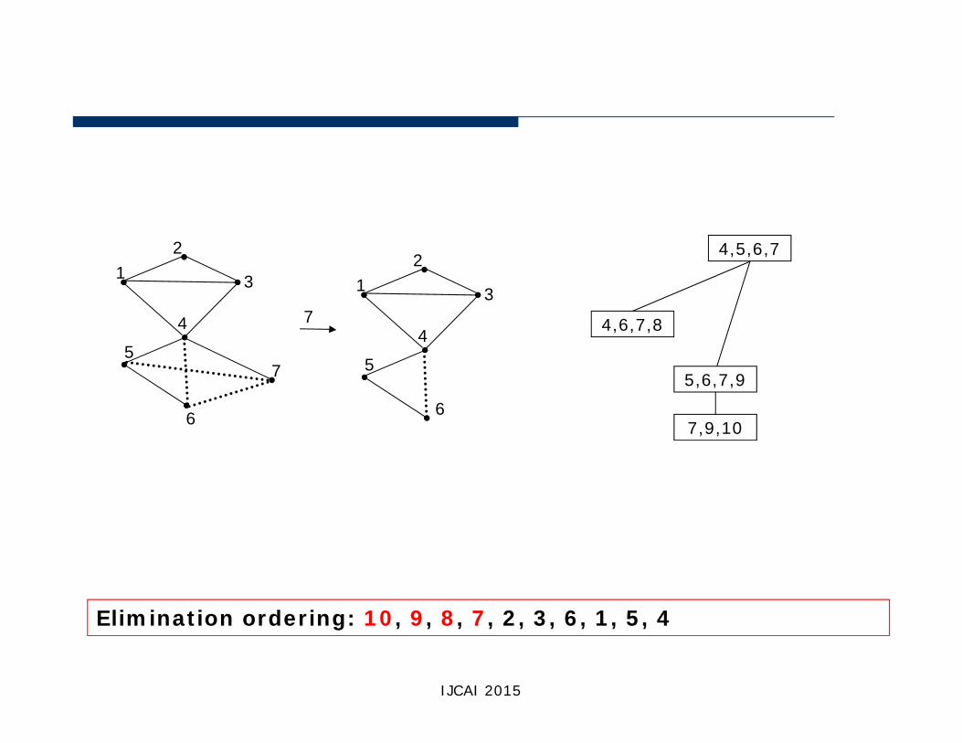
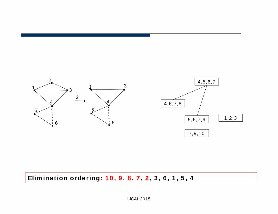
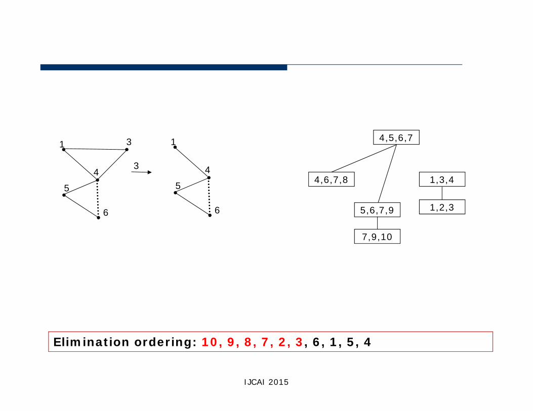
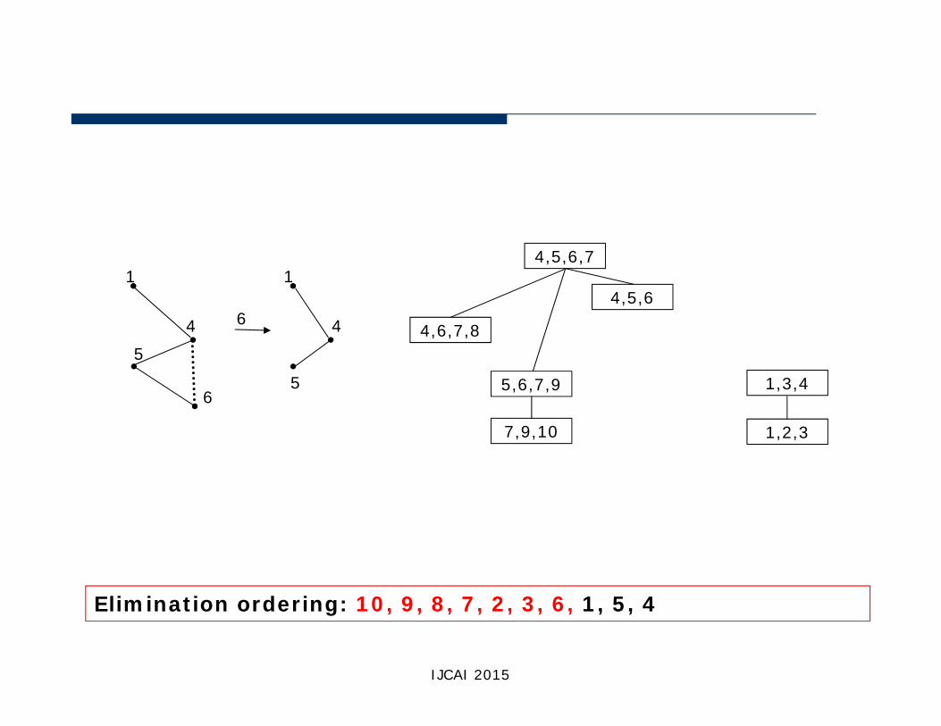
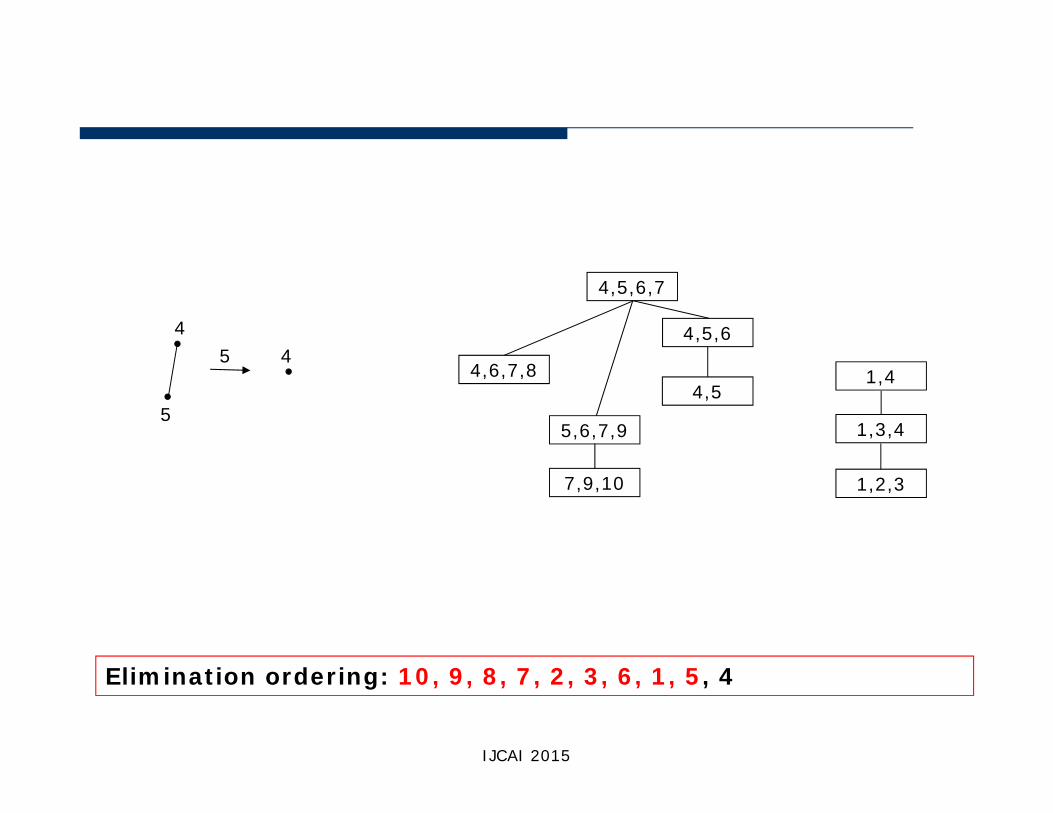
Perfect Elimination Ordering

Vertex 10 is eliminated from the graph. All neighbors of 10 are connected and a tree node is created that contains vertex 10 and its neighbors

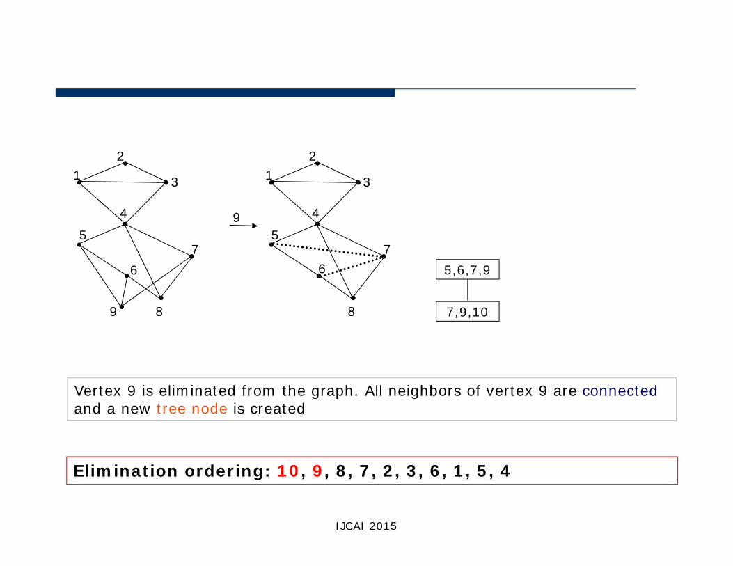
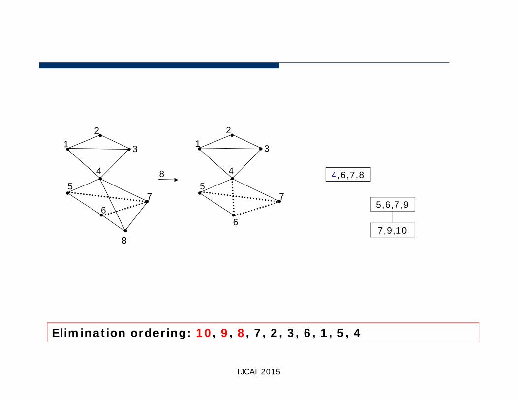
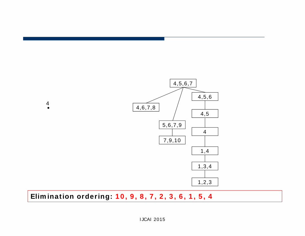
Elimination ordering: 10, 9, 8, 7, 2, 3, 6, 1, 5, 4

2

3

4

5 67

89

10

12

3

45

67

89

10

7,9,10

IJCAI 2015

12

3

45

67

89

12

3

45

67

8

9

7,9,10

5,6,7,9

Vertex 9 is eliminated from the graph. All neighbors of vertex 9 are connectedand a new tree node is created

IJCAI 2015

Elimination ordering: 10, 9, 8, 7, 2, 3, 6, 1, 5, 4

12

3

45

67

8

45

6

7

12

3

8

7,9,10

5,6,7,9

4,6,7,8

IJCAI 2015

Elimination ordering: 10, 9, 8, 7, 2, 3, 6, 1, 5, 4

45

6

7

12

3

74

5

6

12

3

7,9,10

5,6,7,9

4,6,7,8

4,5,6,7

IJCAI 2015

Elimination ordering: 10, 9, 8, 7, 2, 3, 6, 1, 5, 4

45

6

12

3

45

6

1 3

2

7,9,10

5,6,7,9

4,6,7,8

4,5,6,7

1,2,3

IJCAI 2015

Elimination ordering: 10, 9, 8, 7, 2, 3, 6, 1, 5, 4

45

6

1 3

45

6

1

3

7,9,10

5,6,7,9

4,6,7,8

4,5,6,7

1,2,3

1,3,4

IJCAI 2015

Elimination ordering: 10, 9, 8, 7, 2, 3, 6, 1, 5, 4

45

6

1

4

5

1

6

7,9,10

5,6,7,9

4,6,7,8

4,5,6,7

1,2,3

1,3,4

4,5,6

IJCAI 2015

Elimination ordering: 10, 9, 8, 7, 2, 3, 6, 1, 5, 4

7,9,10

5,6,7,9

4,6,7,8

4,5,6,7

1,2,3

1,3,4

4,5,6

4

5

14

5

1 1,4

IJCAI 2015

Elimination ordering: 10, 9, 8, 7, 2, 3, 6, 1, 5, 4

7,9,10

5,6,7,9

4,6,7,8

4,5,6,7

1,2,3

1,3,4

4,5,6

1,4

4

5

45

4,5

IJCAI 2015

Elimination ordering: 10, 9, 8, 7, 2, 3, 6, 1, 5, 4

7,9,10

5,6,7,9

4,6,7,8

4,5,6,7

1,2,3

1,3,4

4,5,6

1,4

4

4,5

4

IJCAI 2015

Elimination ordering: 10, 9, 8, 7, 2, 3, 6, 1, 5, 4

7,9,10

5,6,7,9

4,6,7,8

4,5,6,7

1,2,3

1,3,4

2

3

4

5 67

89

10

IJCAI 2015

Elimination ordering: 10, 9, 8, 7, 2, 3, 6, 1, 5, 4

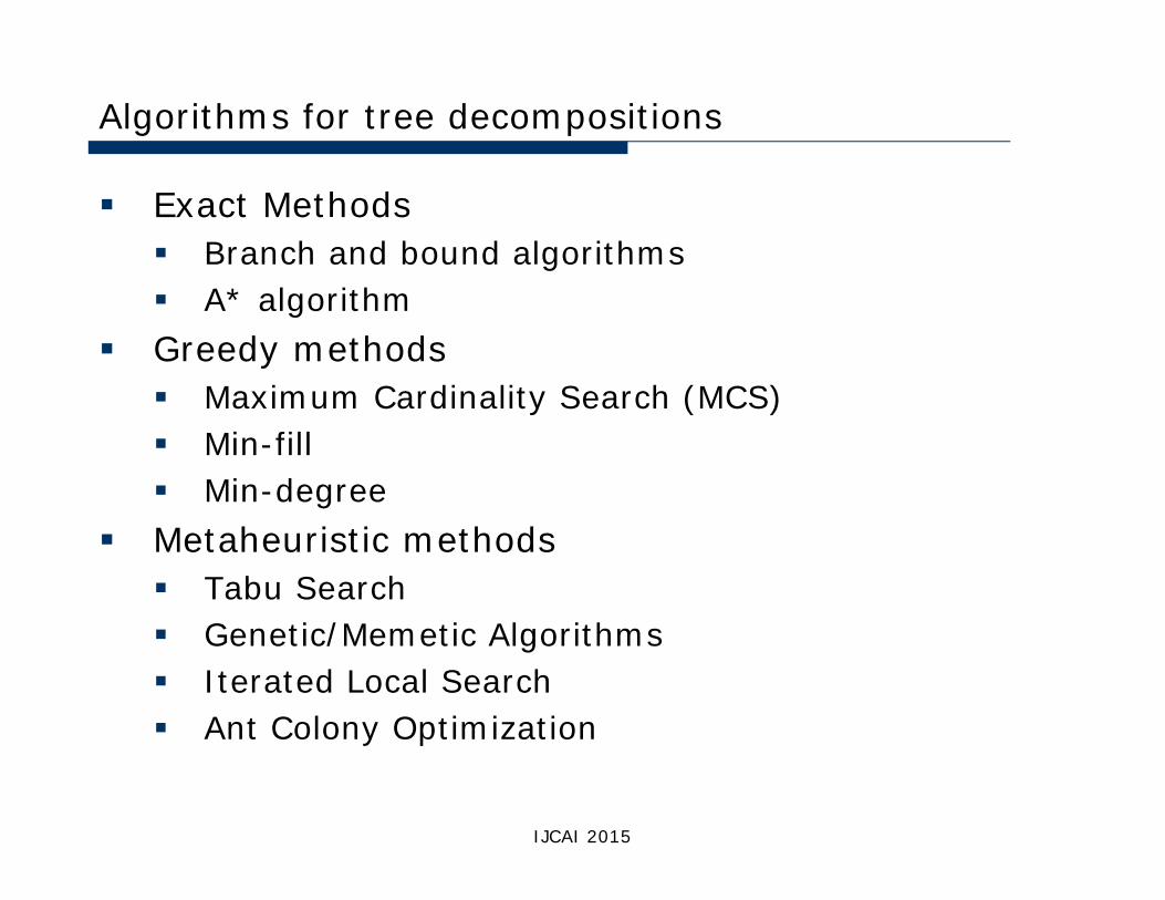
Algorithms for tree decompositions

Exact Methods Branch and bound algorithms A* algorithm

Greedy methods Maximum Cardinality Search (MCS) Min-fill Min-degree

Metaheuristic methods Tabu Search Genetic/Memetic Algorithms Iterated Local Search Ant Colony Optimization

IJCAI 2015

IJCAI 2015

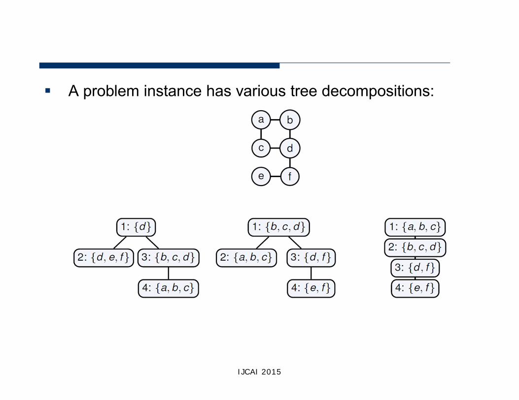
A problem instance has various tree decompositions:

Observation

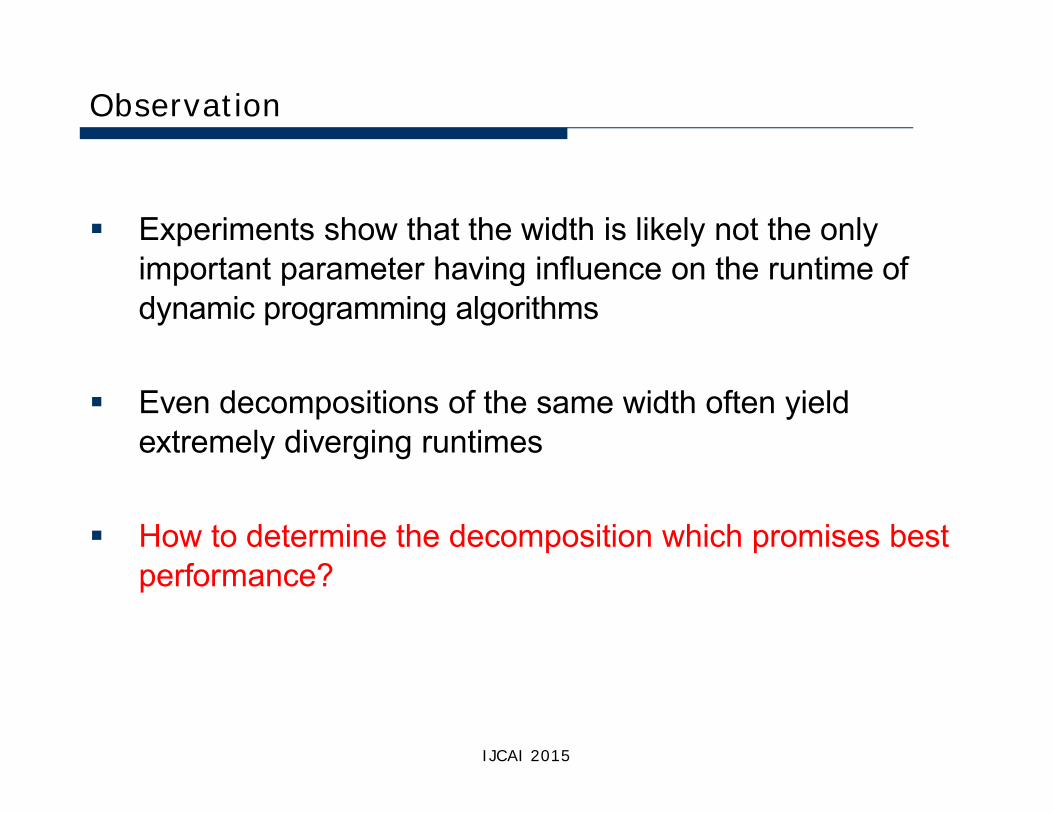
Experiments show that the width is likely not the onlyimportant parameter having influence on the runtime of dynamic programming algorithms

Even decompositions of the same width often yield extremely diverging runtimes

How to determine the decomposition which promises bestperformance?

IJCAI 2015

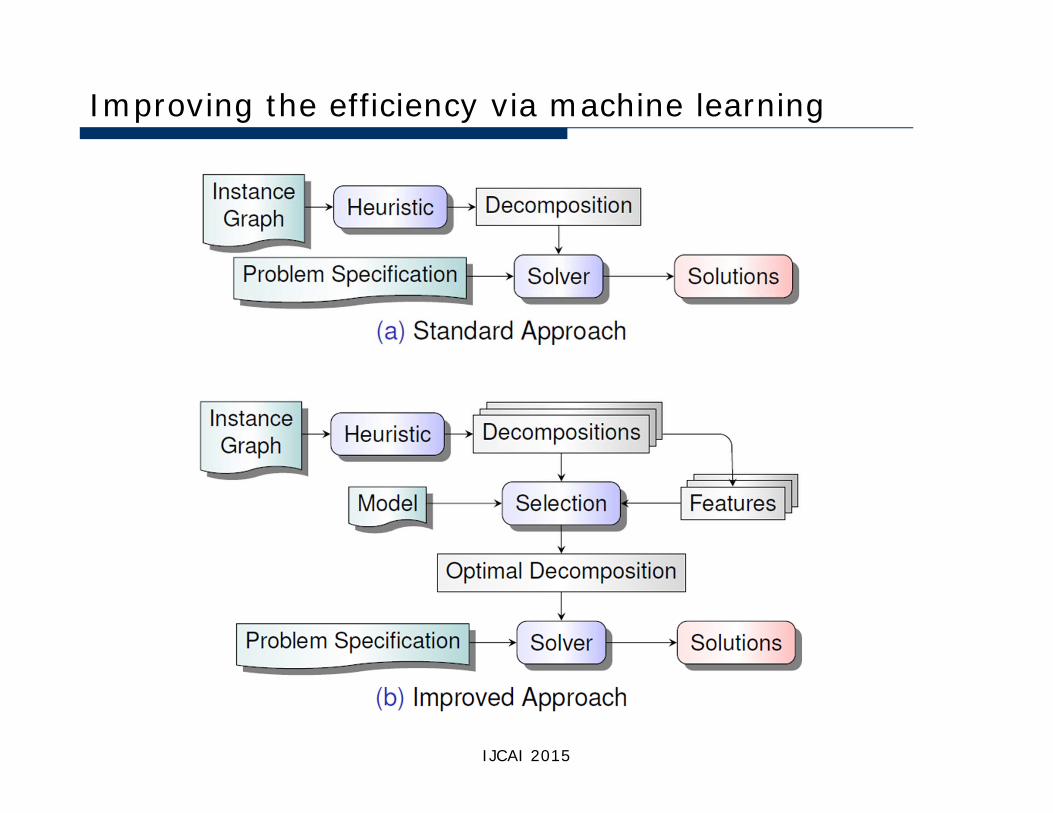
Improving the efficiency via machine learning

IJCAI 2015

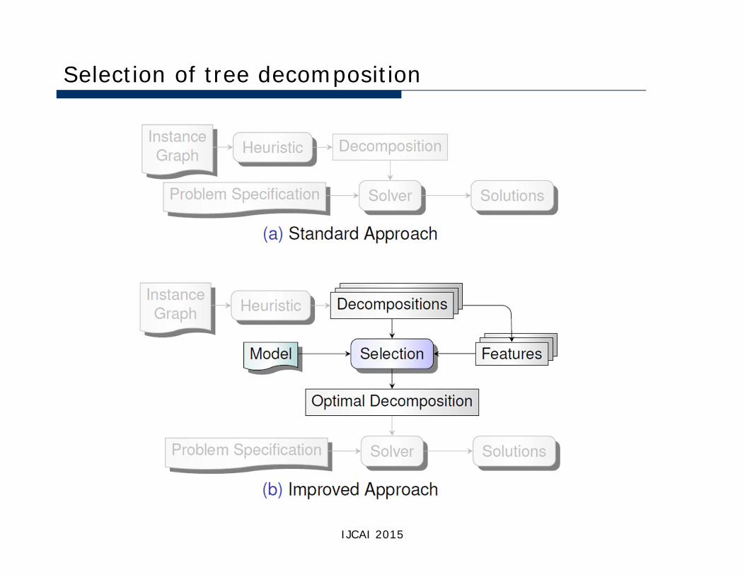
Selection of tree decomposition

IJCAI 2015

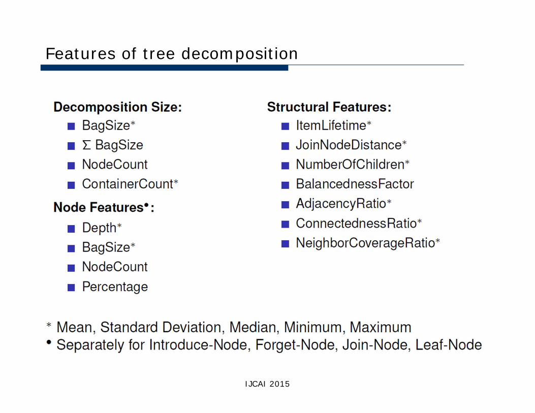
Features of tree decomposition

IJCAI 2015

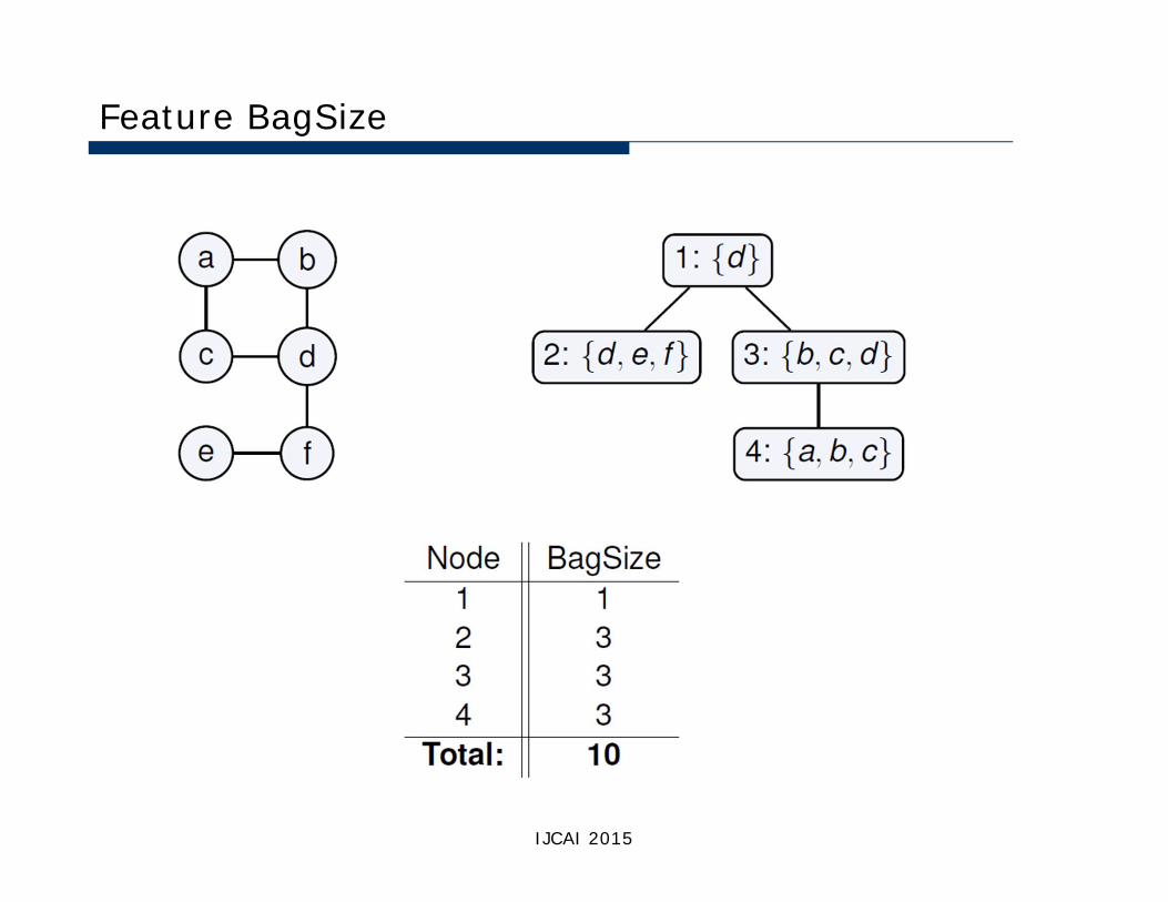
Feature BagSize

IJCAI 2015

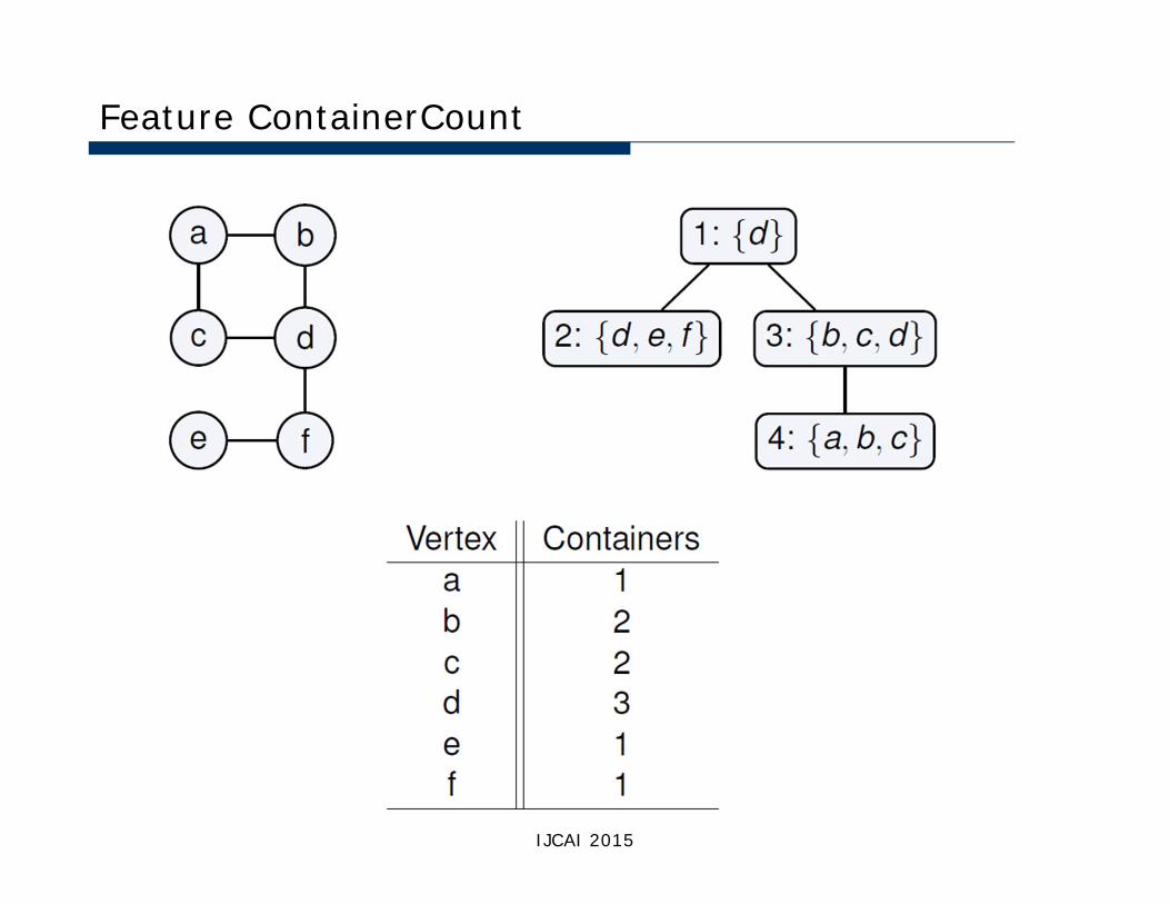
Feature ContainerCount

IJCAI 2015

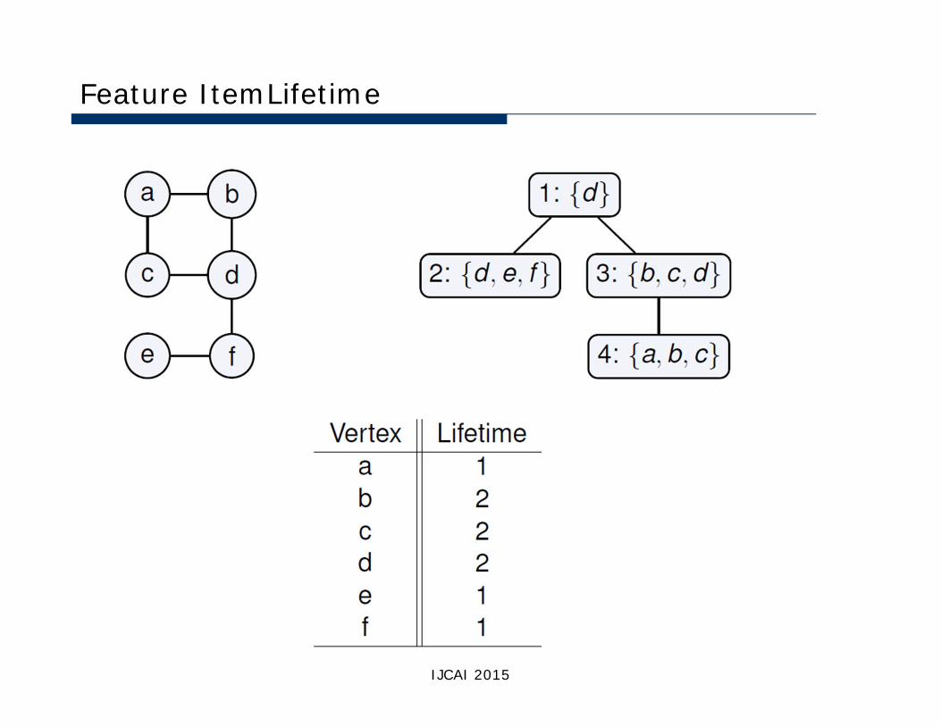
Feature ItemLifetime

IJCAI 2015

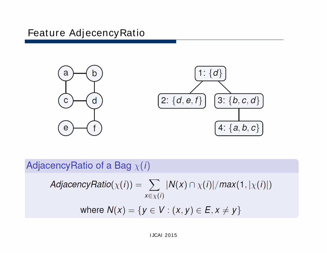
Feature AdjecencyRatio

IJCAI 2015

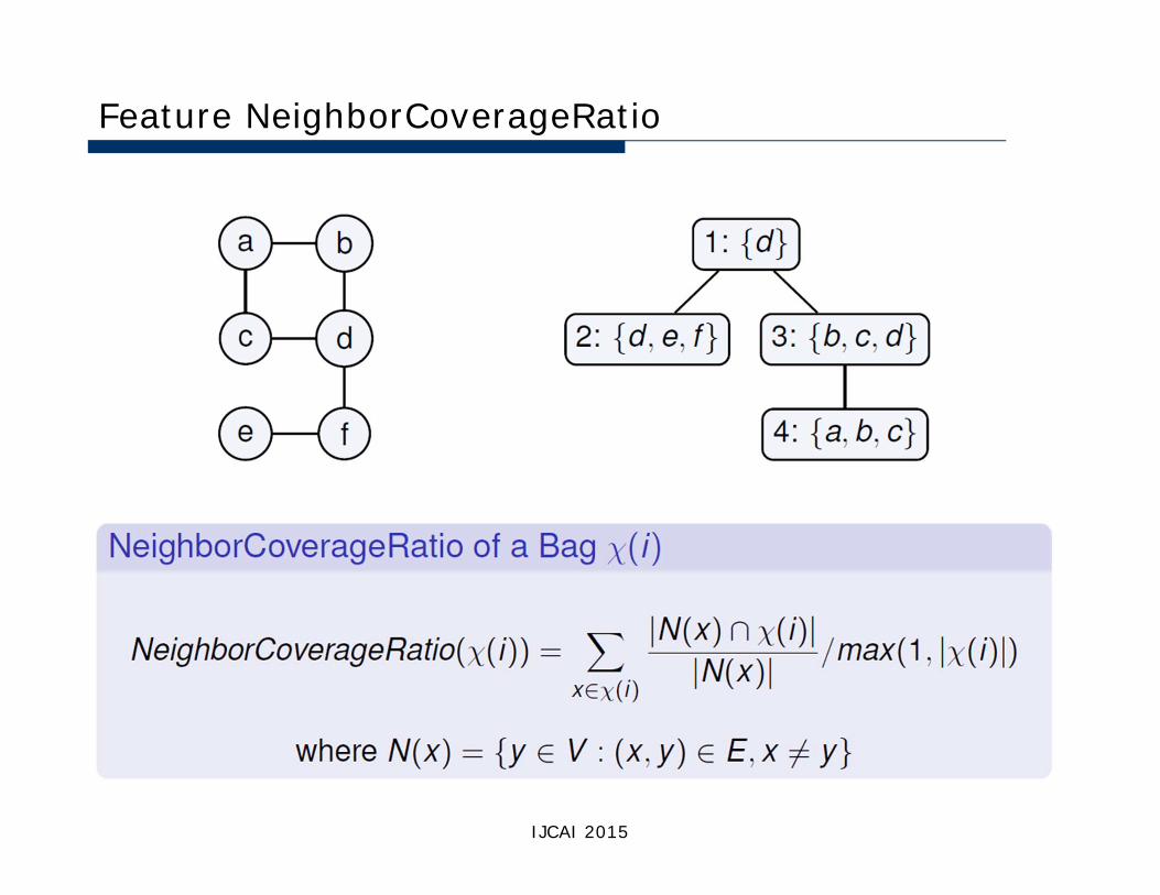
Feature NeighborCoverageRatio

IJCAI 2015

Methodology

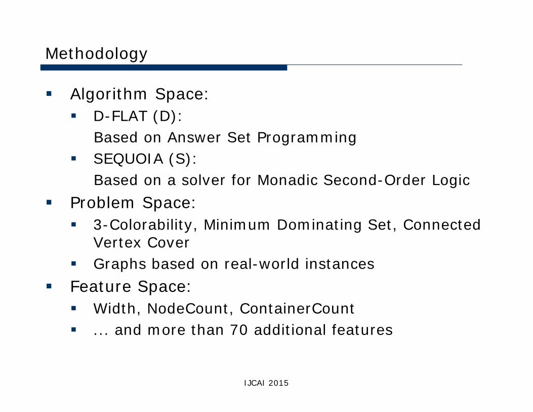
Algorithm Space: D-FLAT (D):

Based on Answer Set Programming SEQUOIA (S):

Based on a solver for Monadic Second-Order Logic Problem Space: 3-Colorability, Minimum Dominating Set, Connected

Vertex Cover Graphs based on real-world instances

Feature Space: Width, NodeCount, ContainerCount ... and more than 70 additional features

IJCAI 2015

Methodology

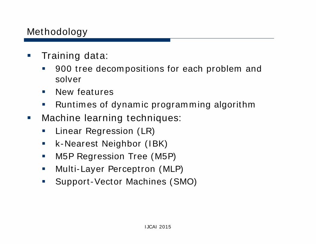
Training data: 900 tree decompositions for each problem and

solver New features Runtimes of dynamic programming algorithm

Machine learning techniques: Linear Regression (LR) k-Nearest Neighbor (IBK) M5P Regression Tree (M5P) Multi-Layer Perceptron (MLP) Support-Vector Machines (SMO)

IJCAI 2015

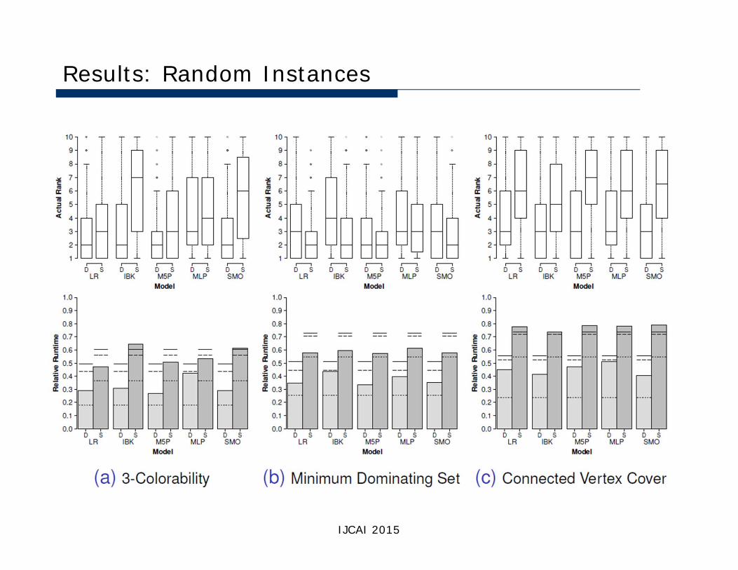
Results: Random Instances

IJCAI 2015

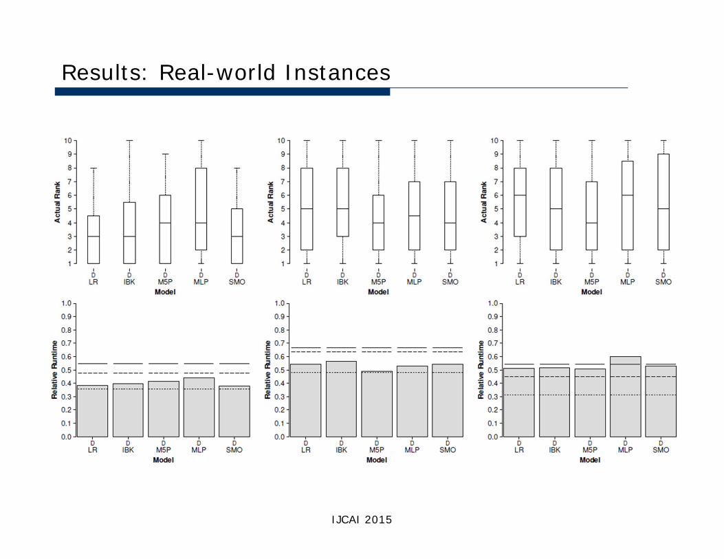
Results: Real-world Instances

IJCAI 2015

Conclusion and Future Work

The width of a tree decomposition is not a reliable measure to predict the runtime of a dynamic programming algorithm in a real-world setting on its own

We determined various features of tree decompositions. Ourexperiments indicate that ... the new features indeed help to find good decompositions computing the novel features is computationally cheap selecting a good decomposition is of negligible effort our concept also pays off in real-world settings

Future work: Investigation of additional problem domains Identification of the most crucial features Ultimate goal: Development of new heuristics for tree decompositions ... which consider the most important features

IJCAI 2015