Problems and Projects - Springer978-0-306-46971-8/1.pdf · Problems and Projects ... an algorithm, a flowchart, executable code in some language, ... the DFT of show that if then

Problems and Projects

The following problems and projects are intended to extend understanding in variousdirections, for example, by proving results in the text, or by applying techniques that arediscussed to specific situations. In some of the projects you are asked to “write” a program ora simulation. This can be interpreted as pseudocode, an algorithm, a flowchart, executablecode in some language, or a “script” in some applications package, as may be appropriate tothe case at hand. Some of the projects are suitable as term projects and could be team efforts.While individual problems are associated with particular chapters, many involve material thatspans the subject matter of several chapters.

Chapter 3

P3.1. Lowpass Equivalent. Write a program to implement a Hilbert transform (a) inthe time domain, (b) in the frequency domain.

P3.2. Lowpass Equivalent for SSB. The Hilbert transform is often used in des-cribing single-sideband modulation (SSB). Show a lowpass equivalent implementation ofsuch a scheme using the Hilbert transform of problem P3.1.

P3.3. Complex Envelope. Let s(t) be a bandpass signal and h(t) a bandpass filter,both more or less arbitrary. Starting from the convolution integral for the output,e(t) = s(t) * h(t), show that the formulation for the output in terms of lowpass equivalentsderived from the Hilbert transform provides the strictly correct solution (i.e., does not dependon bandlimitedness).

P3.4. Complex Envelope. As in Problem P3.3, let s(t) be a bandpass signal and h(t) abandpass filter. The bandpass output is often computed using as the input signal, definedthrough Starting from the convolution integral for the output,e(t) = s(t) * h(t), show that the error in doing so vanishes if s(t) is strictly bandlimited, andobtain thereby integral expressions for the error in this procedure if this is not the case.

P3.5. Sampling. Given a rectangular pulse sampled at a rate(a) compute the ratio of the aliased power to the signal power within the band (b)repeat part (a) for a triangular pulse of the same duration.

P3.6. Prefiltering. It is common to prefilter a signal such as the pulse in problemP3.5 to reduce aliasing. How would you implement such a filter? Discuss the sampling rate

851

852 Problems and Projects

and the bandwidth for the prefilter, and the impact of these parameters on the aliasing.Discuss the tradeoff between aliasing and distortion introduced by prefiltering.

P3.7. Sampling Rate. Let where x(t) is bandlimited toDetermine the proper sampling rate (“small” aliasing error) in terms of B as a function ofConsider (a) a sinusoid of frequency B/2, (b) two sinusoids, the highest frequency being B/2,(c) a bandlimited Gaussian random process.

P3.8. Aliasing. Suppose x(t) is bandlimited with one-sided bandwidth and a filterhas bandlimited transfer function The output of the filter will contain no aliasing error if

where Show that a less stringent condition to produce no aliasingis

P3.9. Aliasing Error. Suppose x(t) is bandlimited to so that that it can berepresented by the usual expansion in terms of sinc functions. Let be a truncated version

Show that the magnitude of the error is given by

where

P3.10. Combined Error Due to Truncation, Aliasing, and Windowing. Let bea real, continuous signal, modeled as a stationary ergodic random process, and let be theimpulse response of a baseband filter. We want to approximate the filter output

with the windowed discrete convolution

where the window W(k) is such that W(k) = 0 for k < 0 and for Now define themean-square error (MSE) as where p is a possible “delay” thatcan be introduced to minimize (a) Show that the MSE is given by

where is the power spectral density (PSD) of is theFourier transform of and is the discrete Fourier transform of (b)

Problems and Projects 853

Obtain reductions of this expression if is bandlimited to and if its PSD iswhite.

P3.ll. Differentiation of a Bandpass Signal. If x(t) is a bandpass signal, and itscomplex envelope is defined through show that

P3.12. Interpolation. Derive Equations (3.5.18) and the specific form for andindicated in the text immediately following.

P3.13. Interpolation. Write a program to implement a third-order spline interpola-tion (or use use a “canned” one), (a) Generate a sequence of randomly spaced samples of awell-behaved function (e.g., by accessing a uniform random number generator; see Chapter 7)and apply spline interpolation to produce a “continuous” curve; (b) apply linear interpolationto the original samples (c) apply parabolic interpolation to the original samples. Superimposeand compare the interpolated curves.

P3.14. Interpolation. Generate samples of a raised-cosine pulse with one-sidedbandwidth where is the bit rate (see Chapter 8). Use a sample spacing

and space the samples on either side of t = 0, spanning bits; i.e., do notsample at the peak of the pulse. Regenerate the raised-cosine pulse using (a) bandlimitedinterpolation (truncated to bits), (b) windowed bandlimited interpolation, (c) linearinterpolation. Suppose you sampled the pulse at t = 0 to make a decision. Calculate therelative error and the impact on the error rate associated with the different interpolationmethods.

P3.15. Multirate Simulation System. Consider the implementation of sampling rateconversion (“multirate”) in a simulation. (a) Describe different kinds of systems wheresampling rate conversion may improve the efficiency of simulation. Draw simulation blockdiagrams showing sampling rate conversion operations as identifiable blocks. (b) For thecases above, calculate the run-time improvement due to multirate simulation. Perform thiscalculation both with and without accounting for the time spent in the sampling rateconversion blocks. (c) Suggest one (or more) efficient approach for the design of interpolatingfilters, [see also M. Pent, L. LoPresti, M. Mondin, and L. Zaccagnini, Multirate samplingtechniques for simulation of communication systems, IASTED International Symposium onModeling, Identification, and Control, Grindewald, Switzerland (February 1987), and VCastellani, M. Mondin, M. Pent, and P. Secchi, Simulation of spread spectrum commu-nication links, Presented at 2nd IEEE Imnternational Workshop on Computer-AidedModeling, Analysis, and Design of Communication Links and Networks, Amherst, Massa-chusetts (October 12–14, 1998)].

P3.16. Discrete Fourier Transform and Fourier Series. Show that the Fourier seriesof a periodic function with period P, bandlimited to where isidentical to the N-point discrete Fourier transform of the function if N > 2M. (Such afunction is called a trigonometric polynomial.)

P3.17. Circular Convolution. If is the DFT of is the DFT of and isthe DFT of show that if then is the circular convolution of and

P3.18. Simulation of a Network Analyzer. Systems are typically characterized bytheir frequency domain response. In practice, such responses are measured using so-called“swept-tone” measurements, performed with a network analyzer. Develop a “discrete-time”network analyzer for your simulation. Discuss the difference between swept-tone and stepped-


tone; also discuss how the analyzer results may be influenced by the relationship between thefrequencies used and the sampling interval.

P3.19. Aliasing and Leakage Effects in the DFT. Consider a sampled version of awaveform, and Comparethe DFT of with the continuous Fourier transform of x(t) for the following conditions:(a) Sampling rate samples/s, T = 20 s, (b) samples/s, T = 64/3 s, (c)

samples/s, T = 10 s, (d) samples/s, T = 32/3 s, and (e) samples/s,T = 64/3 s. Explain the influence of and T on the DFT. How would you mitigate theeffects of aliasing and leakage of a large periodic component in the signal. [See Chapter 3,Refs. 3 and 30, see also A. A. Girgis and F. M. Ham, A quantitative study of pitfalls in theFFT, IEEE Trans. Aerospace Electron. Syst. AES-16, 434–439 (1980).]

Chapter 4

P4.1. Analog Butterworth Filter. Given a lowpass Butterworth filter with a passbandattenuation at the frequency and a stopband attenuation at the frequency determinethe filter order n and the 3-dB bandwidth

P4.2. Relationship between Lowpass Prototype and Lowpass Equivalent. For thelowpass Butterworth filter in P4.1, design a corresponding bandpass filter. Find the lowpassequivalent of this bandpass filter. Compare the lowpass Butterworth filter transfer function tothat of the lowpass equivalent as a function of the ratio of bandwidth to center frequency.Show that, as this ratio the two transfer functions coalesce.

P4.3. Analog Elliptic Filter. Given an analog fourth-order elliptic filter: (a) Find thecoefficient for the biquadratic sections for the normalized lowpass filter with and

and the ratio of the stopband to passband frequencies (b) Show thebiquadratic realization of the filter. (c) Perform a lowpass to bandpass transformation as in(4.1.15) with Hz and (1) (2) (d) Plot thefrequency responses of the lowpass and bandpass filters. (e) Discuss the implications of theband transformations on the lowpass equivalent filter.

P4.4. Bandpass Filter in the Discrete Domain. Given a bandpass filter specified bypoles and zeros, you have to formulate a lowpass-equivalent discrete filter using the impulse-invariant transformation. Under what conditions do the negative-frequency poles not have tobe eliminated?

P4.5. Application of the Bilinear Transform. Provide a discrete model for the filterspecified in problem P4.1 using the bilinear transform with the sampling rates (a) (b)

Discuss the implications. Plot the frequency response and compare with those ofProblem P4.1.

P4.6. Frequency-Domain FIR Filter. How would you determine if an FIR filter hassufficient samples in the frequency domain? (Hint: Obtain the impulse response and integrateits square.)

P4.7. Frequency-Domain Interpolation. Show that augmenting the impulseresponse of an FIR filter with zeros produces interpolating samples in the frequency domain.

P4.8. Gibbs Phenomenon Distortion in an Ideal Filter. Consider a sampled versionof an ideal lowpass FIR filter in the frequency domain (see Figure 4.la). The IFFT produces atruncated impulse response. (a) Explain why the Gibbs phenomenon distortion is invisible in


the frequency domain. (b) Augment the impulse response with zeros and take the FFT.Explain the results.

P4.9. Overlap-and-Add Method. Write a program to implement the overlap and addmethod of filtering.

P4.10. Windowed Response. Redo Problem P4.8 and apply (a) the Hammingwindow (b) the Bartlett window (see also Chapter 10). Compare the results.

P4.11. Filter Synthesis from Measured Data. Given a set of measured ampli-tude and phase points, how would you go about synthesizing an IIR filter from thesepoints?

P4.12. Impulse Response Comparison. For the filter in Example 4.1.7, obtain thediscrete-time filter using the bilinear z-transform. Compare the frequency response, as afunction of to that of the solution given in the example.

P4.13. Gibbs Phenomenon Distortion in a Raised-Cosine Filter. Simulate theraised cosine filter (see Section 8.9) with a frequency rolloff using a frequency-domain FIR filter implementation. What is the Gibbs phenomenon distortion with (a) arectangular window, (b) a Hamming window?

P4.14. Filtering and Multirate. Suppose that you want to filter a signal of bandwidthW with a filter of bandwidth B. (The definition of bandwidth is not critical for this problem.)Even if we know that the bandwidth of the filter output will be at most on the orderof B. Do we still have to generate samples of the input signal (and therefore also samples ofthe filter impulse response) at the rate 2W? What can be done to create efficient sampling atthe filter output on the order of 2B samples/s?

P4.15. Effects of Aliasing and Truncation. Transmit a single rectangular pulse ofduration T into a 0.5-dB ripple three-pole Chebyshev filter withApproximate the filter impulse response by an FIR filter and superimpose the various outputwaveforms computed as a function of the number of samples per unit of T and the length ofthe impulse response.

P4.16. Effects of Aliasing and Truncation. Repeat Problem P4.15 using the bilineartransformation for the same values of sampling rate, and compare the two sets of results.

P4.17. Effects of Aliasing and Truncation. For the filter of Problem P4.15 nowtransmit a short pseudonoise sequence (say 15 bits), using eight samples per bit. (a) Simulateusing an FIR model with and a truncation equal to three time constants. (b) Repeat(a) using a bilinear transformation for the filter, and compare the two resulting sequences.

P4.18. Efficiency of the FFT. It was shown that when using the FFT, the number ofmultiplications for K segments of filtered data is where thenumber of points used in the FFT is N = L + M – 1, L is the actual number of sample points,and M – 1 is the number of padded zeros. Obtain the “effective” number of multiplications

per processed bit, assuming m samples per bit, and taking into account the number ofuseful bits in the OA or OS method. For a given m, plot as a function of N and observe thatthere is an optimum value of N, which depends on M.

P4.19. Impulse-Invariant Transformation. Develop an analytical expression for theimpulse response h(t) of a lowpass five-pole Butterworth filter with 3-dB bandwidth B equalto 1. (a) Obtain the sampled values for (b) Using the pole values,generate the impulse response using a discrete impulse as the input to the impulse-invariantmodel given by (4.1.66), and verify that it is the same as in (a).

P4.20. Filtering with Finite Precision. Generate a sequence of Gaussian randomnumbers with variance equal to 1, at sampling rate and prepare to filter it with a four-pole,0.25-dB-ripple, Chebyshev filter, with cutoff frequency of by using the bilinear trans-


formation. Quantize the generated samples and the filter coefficients at various levels ofquantization (beginning with the “unquantized” values normally produced), and compare thecorresponding filter outputs.

P4.21. Bandwidth Expansion of a Linear Time-Varying System. Show that therelationship in Equation (4.2.8) implies the one in Equation (4.2.9).

P4.22. Discrete LTV Model. Formulate a discrete (sampling) LTV model for a signalwith a bandwidth and an impulse response of Example 4.2.2.

P4.23. Separable LTV Model. Formulate a separable LTV model for the impulseresponse of Example 4.2.2.

P4.24. Inverse of LTV System. The discrete impulse response of an LTV system isgiven in matrix form h(m, n) = A(m, n). Prove that the inverse of the impulse response

is the inverse of the matrix A(m, n). Discuss the practicality of this procedure insimulation.

Chapter 5

P5.1. Nonlinear Spectral Spreading. Assume the output of a nonlinear system isgiven by (5.2.3) for x(t) a finite-energy signal. Show that the output spectrum is given by(5.2.4).

P5.2. Nonlinear Spectral Spreading. Assume you have a pair of AM/AM andAM/PM characteristics (you can create these curves or use published data; see, e.g., those inRef. 10 of Chapter 5). Generate a Gaussian random process and filter it with a filter whosebandwidth is appreciably less than (say, one fifth of) the simulation bandwidth (a) Obtainthe PSD of the filter output (see Chapter 10 for PSD estimation); (b) pass the filter outputthrough the AM/AM characteristic only and obtain the PSD of the output; (c) repeat part (b)using the AM/PM characteristic only; (c) repeat part (b) with both the AM/AM and AM/PMcharacteristics.

P5.3. Nonlinear Spectral Spreading. Repeat Problem P5.2, but instead of a Gaus-sian process, let the input be an unfiltered random binary waveform with at least 16samples/bit.

P5.4. The Chebyshev Transform. (a) Use the substitution A in (5.2.9a) to showthat

is the first term of a Chebyshev expansion of the function F defined over the interval [–A, A].(b) Conclude that if F is an even function: explain in intuitive terms why that is so.

P5.5. Memoryless Nonlinearity. Show that for any “ordinary” function F, thecoefficient defined by (5.2.9b) is always zero.

P5.6. Describing Function of a Hysteresis Nonlinearity. Obtain Equations (5.2.14)starting from the definitions (5.2.9). Hint. Break up the integral into four segments corre-sponding to the four sides of the hysteresis characteristic.

P5.7. Hard-Limiter. Show that for a hard-limiter, the general form (5.2.15) reducesto (5.2.17a) for the baseband case, and implies (5.2.17b) for the bandpass case.


hard-limiter: the output, y(t) = –1 for and y(t) = 1 for x(t) > 0, is sampled at therate samples/s. Examine y(t) in the time and frequency domains. How would youalleviate the anomalous behavior? Consider the effects of sampling rate and sampling phase.

P5.9. Limiter Suppression. Limiters have an effect known as “suppression” wherelarge signals decrease smaller signals. Consider two sinusoids andwith Let and be the corresponding outputs at the original frequencies. Plot theratio versus Make sure you sample sufficiently rapidly.

P5.10. Soft-Limiter, Show that for a limiting amplifier (or soft-limiter), the generalform reduces to (5.2.18a) for the baseband case, and implies (5.2.18b) and (5.2.19) for thebandpass case. Show that (5.2.19) reduces to (5.2.17b) as

P5.11. Asymmetric Limiter. Consider the asymmetric limiter

and

with (a) Obtain the coefficient (b) Show that is still zero, i.e., the asymmetry isnot a factor.

P5.12. Power Series Model. Fill in the steps to show that (5.2.24) is true.P5.13. Effectively Memoryless Nonlinearity. Consider the following model for a

nonlinearity (see Ref. 9, Chapter 5): The input signal is appliedto a memoryless nonlinearity F, then split into N +1 delay lines each with delay

recombined, and passed through a zonal filter. Thus, the output isdescribed by

where means first-zone output. Assume the specific (envelope-dependent) form for the

which shows at least one circumstance under which a model with memory reduces to onewhich is “effectively” memoryless. As stated in the text, “instantaneous” may be a betterterm here.

P5.14. Nonlinear Memoryless Amplifier Modeling. Show that the standard meas-ured AM/AM and AM/PM characteristics, i.e., power out versus power in, and phase outversus power in, can be meaningfully interpreted in discrete time as instantaneous envelope

P5.8. Effects of Finite Sampling. A sinusoidal signal x(t) = A sin is applied to a

delay Show that as and such that the outputreduces to the form


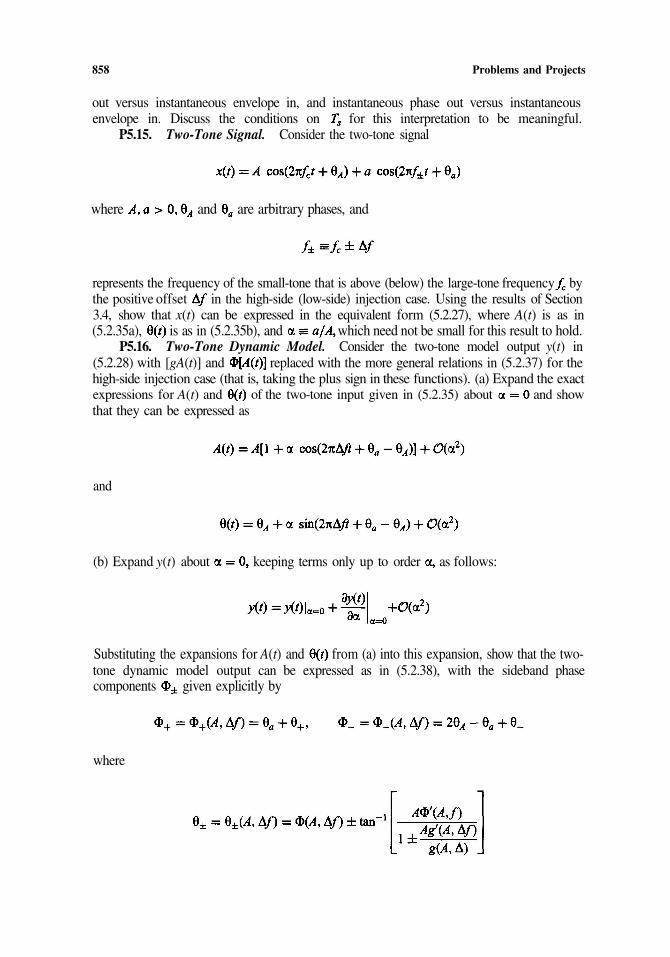
out versus instantaneous envelope in, and instantaneous phase out versus instantaneousenvelope in. Discuss the conditions on for this interpretation to be meaningful.

P5.15. Two-Tone Signal. Consider the two-tone signal

where and are arbitrary phases, and

the positive offset in the high-side (low-side) injection case. Using the results of Section3.4, show that x(t) can be expressed in the equivalent form (5.2.27), where A(t) is as in(5.2.35a), is as in (5.2.35b), and which need not be small for this result to hold.

P5.16. Two-Tone Dynamic Model. Consider the two-tone model output y(t) in(5.2.28) with [gA(t)] and replaced with the more general relations in (5.2.37) for thehigh-side injection case (that is, taking the plus sign in these functions). (a) Expand the exactexpressions for A(t) and of the two-tone input given in (5.2.35) about and showthat they can be expressed as

and

(b) Expand y(t) about keeping terms only up to order as follows:

Substituting the expansions for A(t) and from (a) into this expansion, show that the two-tone dynamic model output can be expressed as in (5.2.38), with the sideband phasecomponents given explicitly by

where

represents the frequency of the small-tone that is above (below) the large-tone frequency by


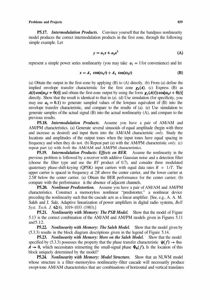
P5.17. Intermodulation Products. Convince yourself that the bandpass nonlinearitymodel produces the correct intermodulation products in the first zone, through the followingsimple example. Let

represent a simple power series nonlinearity (you may take for convenience) and let

(a) Obtain the output in the first-zone by applying (B) to (A) directly. (b) From (a) define theimplied envelope transfer characteristic for the first zone (c) Express (B) as

and obtain the first-zone output by using the formdirectly. Show that the result is identical to that in (a). (d) Use simulation (for specificity, youmay use to generate sampled values of the lowpass equivalent of (B) into theenvelope transfer characteristic, and compare to the results of (a). (e) Use simulation togenerate samples of the actual signal (B) into the actual nonlinearity (A), and compare to theprevious results.

P5.18. Intermodulation Products. Assume you have a pair of AM/AM andAM/PM characteristics. (a) Generate several sinusoids of equal amplitude (begin with threeand increase as desired) and input them into the AM/AM characteristic only. Study thelocations and amplitudes of the output tones when the input tones have equal spacing infrequency and when they do not. (b) Repeat part (a) with the AM/PM characteristic only. (c)repeat part (a) with both the AM/AM and AM/PM characteristics.

P5.19. Intermodulation Products: Effects on BER. Assume the nonlinearity in theprevious problem is followed by a receiver with additive Gaussian noise and a detection filter(choose the filter type and use the BT product of 0.7), and consider three modulatedquaternary phase-shift-keying (QPSK) input carriers with equal data rates R = 1/T. Theupper carrier is spaced in frequency at 2R above the center carrier, and the lower carrier at2.5R below the center carrier. (a) Obtain the BER performance for the center carrier; (b)compare with the performance in the absence of adjacent channels.

P5.20. Nonlinear Predistortion. Assume you have a pair of AM/AM and AM/PMcharacteristics. Construct a memoryless nonlinear “predistorter,” a nonlinear devicepreceding the nonlinearity such that the cascade acts as a linear amplifier. [See, e.g., A. A. M.Saleh and J. Salz, Adaptive linearization of power amplifiers in digital radio systems, BellSyst. Tech. J. 62(4), 1019–1033 (1983).]

P5.21. Nonlinearity with Memory: The PSB Model. Show that the model of Figure5.13 is the correct combination of the AM/AM and AM/PM models given in Figures 5.11and 5.12.

P5.22. Nonlinearity with Memory: The Saleh Model. Show that the model given by(5.3.3) results in the block diagram descriptions given in the legend of Figure 5.14.

P5.23. Nonlinearity with Memory: More on the Saleh Model. Show that the modelspecified by (5.3.3) possesses the property that the phase transfer characteristic as

which necessitates reinserting the small-signal phase Is the location of thisblock uniquely determined by the model?

P5.24. Nonlinearity with Memory: Model Structure. Show that an NLWM modelwhose structure is a filter–memoryless nonlinearity–filter cascade will necessarily produceswept-tone AM/AM characteristics that are combinations of horizontal and vertical translates


of one another on dB scales; and similarly for the AM/PM characteristics with phase thedependent variable and the power axis in dB units.

P5.25. Nonlinearity with Memory: More on Model Structure. Show that the PSBand the Saleh models are generally different. Under what conditions are the models identical(for swept-tone inputs)?

P5.26. Abuelma’atti Model. Show that the Abuelma’atti model does not constrainthe inphase nonlinearities to be horizontal and/or vertical translates of one another(as a function of frequency); and similarly for the quadrature nonlinearities

P5.27. Three-box Model with Least-Squares Fit. In the model of Section 5.3.2.2,the phase of the two filters is ambiguous. Describe some ways in which you might split thederived phase characteristics between the two filters. How might you validate your choice?

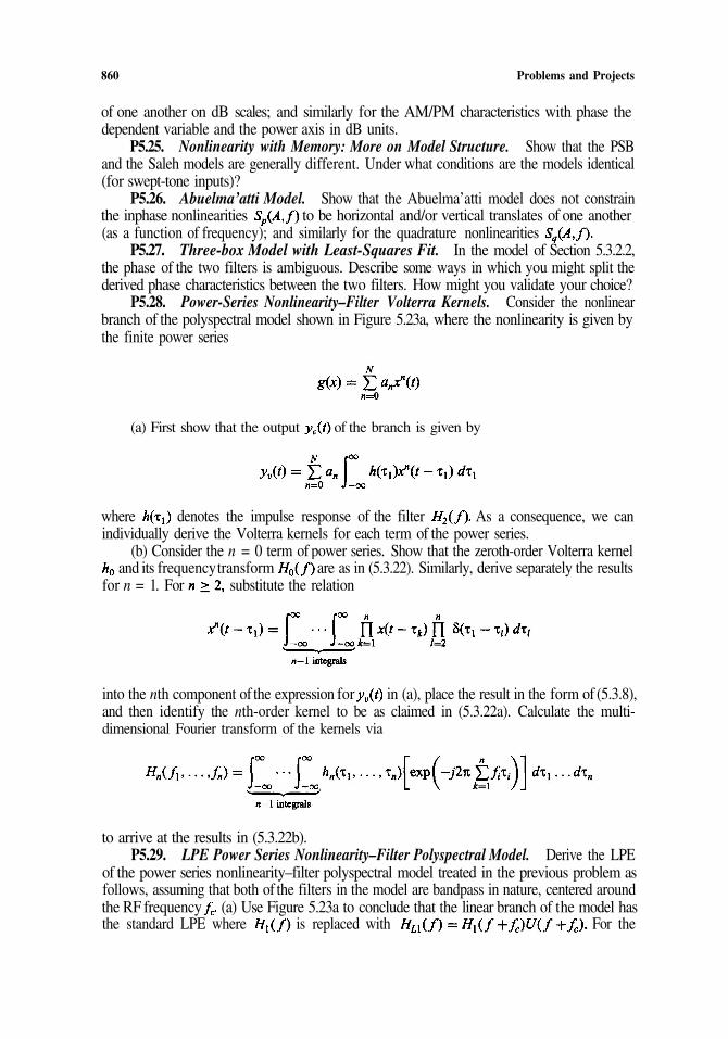
P5.28. Power-Series Nonlinearity–Filter Volterra Kernels. Consider the nonlinearbranch of the polyspectral model shown in Figure 5.23a, where the nonlinearity is given bythe finite power series

(a) First show that the output of the branch is given by

where denotes the impulse response of the filter As a consequence, we canindividually derive the Volterra kernels for each term of the power series.

(b) Consider the n = 0 term of power series. Show that the zeroth-order Volterra kerneland its frequency transform are as in (5.3.22). Similarly, derive separately the results

for n = 1. For substitute the relation

into the nth component of the expression for in (a), place the result in the form of (5.3.8),and then identify the nth-order kernel to be as claimed in (5.3.22a). Calculate the multi-dimensional Fourier transform of the kernels via

to arrive at the results in (5.3.22b).P5.29. LPE Power Series Nonlinearity–Filter Polyspectral Model. Derive the LPE

of the power series nonlinearity–filter polyspectral model treated in the previous problem asfollows, assuming that both of the filters in the model are bandpass in nature, centered aroundthe RF frequency (a) Use Figure 5.23a to conclude that the linear branch of the model hasthe standard LPE where is replaced with For the


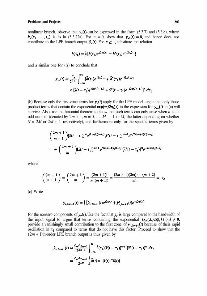
nonlinear branch, observe that can be expressed in the form (5.3.7) and (5.3.8), whereis as in (5.3.22a). For n = 0, show that and hence does not

contribute to the LPE branch output For substitute the relation

and a similar one for x(t) to conclude that

(b) Because only the first-zone terms for apply for the LPE model, argue that only those

where

(c) Write

for the nonzero components of Use the fact that is large compared to the bandwidth ofthe input signal to argue that terms containing the exponential

oscillation in compared to terms that do not have this factor. Proceed to show that the(2m + l)th-order LPE branch output is thus given by

product terms that contain the exponential in the expression for in (a) willsurvive. Also, use the binomial theorem to show that such terms can only arise when n is anodd number (denoted by 2m + 1, m = 0, . . . , M – 1 or M, the latter depending on whetherN = 2M or 2M + 1, respectively), and furthermore only for the specific terms given by

provide a vanishingly small contribution to the first zone of because of their rapid


where * denotes the convolution operation. Conclude that the LPE of the nonlinear branch is

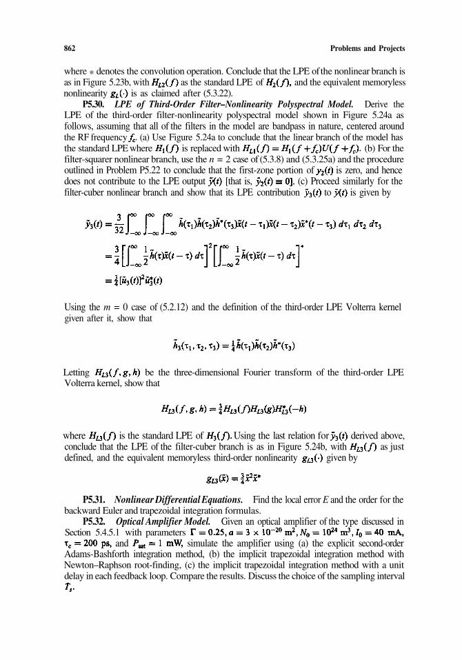
nonlinearity is as claimed after (5.3.22).P5.30. LPE of Third-Order Filter–Nonlinearity Polyspectral Model. Derive the

LPE of the third-order filter-nonlinearity polyspectral model shown in Figure 5.24a asfollows, assuming that all of the filters in the model are bandpass in nature, centered aroundthe RF frequency (a) Use Figure 5.24a to conclude that the linear branch of the model hasthe standard LPE where is replaced with (b) For thefilter-squarer nonlinear branch, use the n = 2 case of (5.3.8) and (5.3.25a) and the procedureoutlined in Problem P5.22 to conclude that the first-zone portion of is zero, and hencedoes not contribute to the LPE output [that is, (c) Proceed similarly for thefilter-cuber nonlinear branch and show that its LPE contribution to is given by

Using the m = 0 case of (5.2.12) and the definition of the third-order LPE Volterra kernelgiven after it, show that

Letting be the three-dimensional Fourier transform of the third-order LPEVolterra kernel, show that

conclude that the LPE of the filter-cuber branch is as in Figure 5.24b, with as justdefined, and the equivalent memoryless third-order nonlinearity given by

P5.31. Nonlinear Differential Equations. Find the local error E and the order for thebackward Euler and trapezoidal integration formulas.

P5.32. Optical Amplifier Model. Given an optical amplifier of the type discussed inSection 5.4.5.1 with parameters

and simulate the amplifier using (a) the explicit second-orderAdams-Bashforth integration method, (b) the implicit trapezoidal integration method withNewton–Raphson root-finding, (c) the implicit trapezoidal integration method with a unitdelay in each feedback loop. Compare the results. Discuss the choice of the sampling interval

as in Figure 5.23b, with as the standard LPE of and the equivalent memoryless

where is the standard LPE of Using the last relation for derived above,


Chapter 6

P6.1. Moments of Sums of Random Variables. The estimator of the mean of a ran-dom variable has the form

where are N independent samples from the underlying pdf . Assuming the underlyingpdf is N(0,1), find the mean and variance of the estimator Y.

P6.2. Moments of Sums of Random Variables. The estimator for the variance of azero-mean Gaussian has the form

Find the mean and variance of the estimator in terms of the unknown variance of theunderlying pdf of X and the sample size N.

P6.3. Moments of Sums of Random Variables. Suppose the sampled values of theoutput of the receive filter in a communication system has the form

where is an independent sequence of octal symbols with values –7, –5, –3, –1, 1, 3, 5,and 7, and represents sampled values of the impulse response with values

and Compute the first eight moments of the ISI.P6.4. Transformation of Random Variables. Transformations of random variables

are used for generating random numbers. Find the pdf of the following transformations: (a)Y = – log(X), where X is uniform in [0, 1]. (b) where X is Gaussian (0, 1).(c) where and are independent Gaussian (0, 1) variables.

P6.5. Vector-Valued Transformations. and are two independent, zero-mean,unit-variance Gaussian variables. and are defined by the transformations

and

Find the joint pdf of and and the marginal pdf’s of andP6.6. Bounds and Approximations. Plot the Chebyshev and the Chernoff bounds as

well as the exact values for P[X > a] versus a, a > 0, for the following pdf’s of X: (a)Uniform [0, 1]. (b) Exponential. (c) N(0, 1).

P6.7. Bounds and Approximations. Derive the union bound for the MPSK systemin which the decision metric has the form Z= X + N, where X is a complex signal havingvalues that are uniformly spaced on a circle of radius1, 2 , . . . , M – 1), with equal probability, and is a complex noise sample whosecomponents are uncorrelated zero-mean Gauassian variables with a variance Express theprobability of error as a function of and M.

P6.8. Bounds and Approximations. Repeat the previous problem for a 16-QAMconstellation in which the complex signal component X has 16 equally likely values whichare uniformly spaced at the corners of a rectangular grid X = mA +jnA,m,n = –3, –1, 1,3.


P6.9. Sampling Rate. Suppose we want to sample a zero-mean Gaussian processwith the autocorrelation function Compute the signal to aliasing powerratio as a function of sampling rate normalized by (e.g., for

P6.10. Noise Bandwidth of Filters. Compute the noise bandwidth of a Butterworthfilter of order 2, 4, 6, 8, 10. Assume that the filters have a 3-dB bandwidth of 1 Hz.

P6.11. Noise Bandwidth of Filters. Consider a simple analog filter with an impulseresponse of for t > 0. (a) Compute the noise bandwidth of the analog filter. (b)Suppose the analog filter is simulated as an IIR filter using a sampling rate of n samples/s.What is the noise bandwidth of the filter for n = 10,20, 50, and 100? (c) Suppose the filter issimulated as an FIR filter using a truncated impulse response of N samples, N = 2n, 8n, and16n, where n is the sampling rate. Find the noise bandwidth as a function of n and N. Explainthe results.

P6.12. Lowpass-Equivalent Representation. Consider a bandpass system in whichthe received radiofrequency signal has the form Y(t) = X(t) + N(t), where X(t) =

is the signal component, is uniform in and N(t) is bandlimitedGaussian noise with a PSD of in the interval and 0 elsewhere

(a) Find the lowpass-equivalent representation in the time domain and frequencydomain for the signal and noise components. (b) Find the signal to noise power ratio, definedas for the bandpass and lowpass representations. Are they the same for thetwo representations?

P6.13. Lowpass-Equivalent Representations. Consider a complex bandlimitedGaussian process n(t) with a power spectral density

Find the lowpass-equivalent representation of n(t) of the form That is,find the power spectral densities of the quadrature components and also the cross-correlationbetween them.

P6.14. Quantization Effects. Finite-precision arithmetic may affect simulation andimplementation accuracies. Suppose we are simulating an FIR filter of the form

(a) If the are independent random variables with a uniform pdf in theinterval [0, 1] and find the output pdf. (b) If the and the are quantized to eightlevels over their respective ranges, find the mean and variance of Y and the mean square errordefined as

where is the quantized version of the output.P6.15. Response of Linear Systems to Random Inputs. The input to a second-order

Butterworth filter with a 3-dB bandwidth of 4 kHz is a lowpass Gaussian process with a two-sided psd of over –4000 <f < 4000 and 0 elsewhere. Find the mean and variance ofthe output of the filter.

P6.16. Response of Nonlinear Systems to Random Inputs. The input X(t) to amemoryless nonlinearity is a real-valued, lowpass, Gaussian process with a two sided PSD


for and 0 elsewhere. Find the mean, variance, and the pdf of the output of thenonlinearity for the following cases:

Chapter 7

P7.1. Uniform Random Number Generator. Implement the following algorithms forgenerating uniform random numbers: (a) Linear congruential. (b) Wichman–Hill algorithm.(c) Marsaglia–Zaman algorithm.

P7.2. Uniform Random Number Generators. Compare the histograms of the outputof the above three algorithms using 1 million samples and 100 bins of width 0.01. Do thecomparison visually by plotting the histograms and by applying the chi-square goodness-of-fittest with

P7.3. Uniform Random Number Generators. Prove that the period of a randomnumber generator defined by a recursion, such as the linear congruential, Wichman–Hill, andMarsaglia–Zaman generators, must have a finite period.

P7.4. Uniform Random Number Generators. (a) Show that the period of a linearcongruential generator of modulus M can have a period of at most M; (b) show that amultiplicative linear congruential generator with prime modulus M has period equal toM – 1.

P7.5. Exponential. Write a program to generate exponentially distributed randomnumbers; use the transform method.

P7.6. Rayleigh. Repeat problem 7.5 for Rayleigh distribution.P7.7. Discrete RV. Write programs to generate random numbers from the following

discrete distributions: (a) gamma (b) Poisson (c) geometric (d) binomialB(n, p).

P7.8. Gaussian. Write a program to generate samples from a Gaussian distributionusing the Box–Muller method.

P7.9. Arbitrary pdf. Assume that X is a continuous random variable with a pdfdefined on a finite interval [a, b]. Write a program to generate samples of X using the methoddescribed in Figure 7.4. Assume uniform quantizing.


P7.10. Gaussian. Write a program to generate Gaussian random variables using theinverse transform method and the following approximation for the distribution function:

where andP7.11. Computational Efficiency. Compare the computational efficiency of the

Gaussian random number generators described in (7.2.6) and Problems 7.8 and 7.10, i.e.,generate, say, 10,000 samples using each method and compare the run times.

P7.12. Discrete RV. Assume that X is a discrete random variable andGiven write a program to generate

samples of X.P7.13. Acceptance/Rejection Method. Assume that analytical expressions are given

for a pdf and a bounding function and the inverse cumulative Write aprogram to generate samples of X using the acceptance/rejection method.

P7.14. Random Binary Sequence. Write a program to generate a random binarysequence using the uniform RNG with P(X = 0) = p and P(X = 1) = 1 – p.

P7.15. Binary PN Sequence. Write a program to generate binary PN sequences forregister lengths ranging from 6 to 16.

P7.16. M-ary PN Sequence. Write a program to generate octal and quaternary PNsequences for register lengths ranging from 2 to 5.

P7.17. Colored Gaussian Process. Write a program to generate sampled values ofzero-mean white Gaussian noise with a given power spectral density (use a frequency-domainfilter).

P7.18. Correlated Gaussisan Sequences. Derive the algorithm for generating aGaussian vector with a mean vector of zero and a covariance matrix givenby [each component process is white]

P7.19. Correlated Gaussian Sequences. Consider a bandlimited complex Gaussianprocess with a power spectral density

For the lowpass-equivalent representation of n(t) of the form find thepower spectral densities of the quadrature components and also the cross-correlation betweenthem. Develop a procedure for generating sampled values of the complex samples of thelowpass-equivalent process.


P7.20. Gaussian Process with arbitrary PSD. Generate a temporally correlatedsequence of samples from a zero-mean Gaussian process with a PSD

and zero elsewhere

(this is the so-called Jakes Doppler spectrum used in modeling the Doppler spectrum inmobile communication channels). Assume that can range from 10 to 100 Hz. Choose anappropriate sampling rate and implement the spectral shaping filter as an FIR filter.

P7.21. Gaussian Process with a Specified Autocorrelation Function. Suppose wewant to generate sampled values of a Gaussian process with an autocorrelation function

Choose an appropriate sampling rate as a function of and develop a10th-order AR model for generating sampled values of the process. (Find the coefficients ofthe AR model using sampled values of the autocorrelation function in the Yule–Walkerequations.)

P7.22. Chi-Square and KS Tests. Write a program to implement the chi-square andKS goodness-of-fit tests. Assume that the histogram intervals, counts, and the underlying truebin probabilities will be specified by the user in a table form. Yourprogram should read a file containing N sampled values of the output of the RNG and applythe chi-square and KS tests at a user-specified value for the significance level.

P7.23. Correlation. Write a program to compute the cross-correlation between twovectors X and Y of dimension N. The output should be an array of the normalized correlationcoefficients defined as

(See Chapter 10 for a DFT-based procedure.)P7.24. Correlation. Let X(k) and Y(k) be two random sequences with Y(k) =

aX(k – m). Derive a procedure for estimating a and m and write a program to implement it (ais a positive constant, m is a positive integer).

P7.25. Correlation. Generate a sequence of 10,000 independent Gaussian numbers.Compute and plot the normalized autocorrelation function of the sequence for lags rangingfrom 0 to 9500 for three different seeds. Does the RNG exhibit any significant correlation?Do the results differ much as a function of the seed?

P7.26. Correlation Test. Generate Y(k) = X(k) + X(k + 100), k = 1,2, . . . , 10,000.Apply the correlation test to Y(k).

P7.27. Miscellaneous. Suppose the intersysmbol interference in a communicationsystem can be expressed as

where is an independent sequence of octal symbols with values –7, –5, –3, –1, 1, 3, 5,and 7, and represents sampled values of the impulse response with values

and Generate a PN sequence of appropriate length that willproduce all possible ISI values. Obtain a histogram of the ISI values. Could the ISI distri-bution be approximated by a Gaussian? (use the chi-square goodness-of-fit test).


Chapter 8

P8.1. Multitone Source Model. Multiple sinusoids (tones) are sometimes used as asource model. One source that can be emulated by multiple tones is a “white noise load,”which is a band of uniform-PSD Gaussian noise with “notches.” Study via simulation theapproach of to a normal distribution, as a function of N. The phases

by the coordinates where These ideal locationscannot be exactly realized in hardware. Develop a specification for an actual modulator interms of a maximum tolerance around each point in the constellation. Assuming an idealchannel and demodulator, establish the degradation in BER performance as a function of thetolerance for two cases: (a) the “worst-case” degradation, and (b) the degradation when theactual symbol location is uniformly distributed over the tolerance range.

P8.7. Quadrature Modulation/Demodulation. Consider the following system. AQAM modulator generates a signal which is sentthrough a linear bandpass channel with transfer function The demodulator multipliesthe received signal by to produce the in-phase baseband signal and by

to produce the quadrature baseband signal The angle is a demodulatorreference error (static phase error). (a) Show that the output signals are given by

where and and

where and are, respectively, the real and imaginary parts of the lowpass-equivalentimpulse response. (b) Express and in terms of the real and imaginary parts of the

are independent and uniformly distributed on Discuss the influence of the on theGaussianness and on the spectral density of the sum.

P8.2. Convolutional Encoder. Write a program to implement a general convolu-tional encoder.

P8.3. Viterbi Decoding. Write a program to implement a “practical” version of theViterbi algorithm; i.e., use soft decisions, truncated path memory, etc. Test your program on asystem model.

P8.4. Frequency Modulation. Write a program to simulate a frequency modulator.Interpreting the FM modulator as a nonlinear device (why?), discuss the required samplingrate.

P8.5. M-ary QAM Signal Generation. Assume you have available in your libraryonly binary sequence generators. You want to simulate an M-QAM signal, where M is aperfect square. Show that you can build up an M-QAM modulator hierarchically. In particular,(a) show that you can build a QPSK modulator from two binary sequence generators, and (b)show that you can build a 16-QAM modulator from two QPSK modulators.

P8.6. Modulator Specification for M-QAM. Consider a 64-QAM signal whoseconstellation has the appearance of Figure 11.36. The ideal location of the symbols is given


lowpass-equivalent transfer function. [Hint: Use odd and even decomposition (see Section3.4).]

P8.8. The Complex Envelope of CPM Signals. Write a program to generate thecomplex envelope of CPM signals. Discuss the required sampling rate.

P8.9. MSK Modulation. A pictorial representation of the possible values of thecomplex envelope is often called a signal space diagram, examples of which are shown inFigure 8.14. (a) Show that the signal space diagram for MSK is a circle. Label the transitionfrom quadrant to quadrant with the corresponding symbol transitions. (b) Write a program toimplement MSK in quadrature form. (c) Obtain a signal space diagram from your simulation.

P8.10. Trellis-Coded Modulation. (a) Write a program to implement a (Ungerboeck)trellis encoder using an 8-ary PSK signal constellation and a Viterbi decoder. For a code withparity-check matrix [see, e.g., R. E. Blahut, Digital Transmission of Infor-mation, Addison-Wesley, Reading, Massachusetts (1990), pp. 272–273, for the interpreta-tion], an AWGN channel, and matched filter detection in the receiver, plot simulated BER vs.

for soft decision quantized to 4 and 8 bits; (b) obtain the BER as in part (a), as afunction of phase error; (c) place a transmission filter in the path of the signal (to create ISI)and repeat parts (a) and (b); (d) draw the trellis for enough branches to obtain the free distance

and the number of paths possessing that distance; (e) compare the various results to thefirst-order approximation for the BER, where m is the number ofbits/symbol and the average number of bit errors on the divergent paths of distance

P8.11. Frequency Demodulation. Write a program to implement the following typesof frequency demodulator: (a) A discriminator; this device ideally extracts the derivative ofthe phase of the input; (b) a delay-line discriminator. For the above demodulators, obtain viasimulation the output SNR versus the input SNR curve for sinusoidal tone signal. (Hint:There are different ways to implement differentiation in discrete time; see, e.g. Ref. 41 inChapter 8.)

P8.12. Discrete-Time Differentiation. Prove that a bandlimited differentiator has thediscrete-time impulse response given by (8.8.16).

P8.13. Discrete-Time Differentiation. Obtain Equation (8.8.20) and the coefficientvalues when m = 3. Form the table of divided differences for the coefficients

P8.14. Discrete-Time Differentiation. Consider a random process X(t) with powerspectral density Pass X(t) through an ideal differentiator:Y(t) = dX(t)/dt. Assume X(t) and Y(t) are sampled at a rate samples/s to form discrete-time sequences. Plot the signal-to-aliasing noise ratio for both X(t) and Y(t) as a function of

P8.15 Equalizer Convergence. (a) Show that the MSE for a tapped-delay-lineequalizer is a convex function of the tap gains. (b) Discuss the implications for equalizerconvergence. (c) Write a program to implement an MSE equalizer. (d) Experiment with theinitial values of the tap coefficients and the coefficient step sizes.

P8.16 Equalizer Implementation. Some systems employ baseband equalizers andsome use IF (intermediate-frequency) equalizers. Assume a QAM system. (a) Draw the actualblock diagram for each type. (b) Draw the simulation (lowpass-equivalent) block diagram foreach type.

P8.17 Equalizer Tap Spacings. (a) Discuss the properties of the MSE equalizer as afunction of the tap spacing (b) Discuss the implications of for the simulation of theequalizer. (Hint: Consider the symbol synchronization aspect of the relation between andTs.)


P8.18 Equalization of Static Phase Error. (a) Show that a TDL equalizer willalways compensate for static phase error. (b) In an otherwise undistorted system, how manytaps are required?

P8.19 Baseband Equalization by Channel Covariance Matrix Inversion. Considera baseband four-level PAM signal operating through a linear channel with finite impulseresponse Find the optimal tap gains for an MMSEequalizer by the covariance matrix inversion method. What should be the number of taps ofthe equalizer?

P8.20 Bandpass Equalization by Channel Covariance Matrix Inversion. Considera QPSK system. The channel is linear. Assume the channel transfer function is represented bya five-pole, Chebyshev bandpass filter, with and where

is the passband ripple parameter, is the passband edge frequency, is the symbol rate,and is the carrier frequency. (a) Obtain the (complex) response to a unit pulse at the input tothe I channel. (b) Find the optimal (complex) tap gains for a 5-tap, 7-tap, and 9-tap MMSEequalizer by the covariance matrix inversion method. (c) Evaluate the BER with and withoutequalization using a QA technique (see Sections 11.2.7 and 12.1).

P8.21. Equalized Mean-Square Error. Show that the minimum mean-squared errorof the LMS equalizer is given by (8.9.37).

P8.22 PSK Demodulation Phase Ambiguity Resolution. (a) Show that data-derivedphase estimation for M-ary PSK using an Mth-power loop produces an M-fold ambiguity. (b)How would you implement your simulation so as to resolve this ambiguity?

P8.23 Binary CPFSK Demodulation. Consider a binary CPFSK signal withdeviation ratio h = n/m, where n, m are integers. (a) Show that, in principle, a phase andtiming recovery structure can be implemented by first raising the signal to the mth power,followed by two phase-locked loops centered at where is the carrier frequencyand T the symbol duration. The PLLs are followed by a multiplier, the output of which is fedto two bandpass filters, one at and the other at n/T. Show the block diagram, includingthe processing following the bandpass filters that must be done to recover the carrier and theclock. (b) How might you implement such a structure in simulation without explicitlysimulating phase-locked loops (treat them as narrowband filters)?

P8.24 Phase Noise Equivalent Process. The residual phase noise in a demodulatedsignal is due to the sum of tracked thermal noise and untracked oscillator noise. Write aprogram to generate this residual noise (assuming its statistics are Gaussian) by using a“white” noise source and appropriate filtering; assume your specifications are a spectralshape and an rms value for each component.

P8.25 Phase Noise and Block Coding. Show that correlated noise, such as phasenoise, has a worse effect on block-coded performance than “wideband” noise. Consider thecase of an idealized OQPSK system only AWGN corrupts the system, except for phase noiseat the demodulator; prior to the decision device. Formulate the (average) probability of biterror for a block-coded system with hard decisions. Postulate a reasonable decoding rule. Forsimplicity you may assume the correlated noise is slow enough to remain essentially constantover a code block.

P8.26. Carrier Phase Synchronization. Develop a lowpass-equivalent simulation toobtain the behavior of a “times-four” loop. Consider the use of multirate techniques, asappropriate. The system configuration is as follows. The input r(t) is the sum of a QPSKsignal s(t) and additive white Gaussian noise n(t). This sum is input to a “front-end” filterwith transfer function then into a “quadrupling device,” which delivers Thissignal is input to a narrowband filter the output of which is the input to a second-order


PLL with The carrier frequency is initially the same as the rest frequency of theVCO, and the latter is assumed ideal. (a) Plot the phase error as a function of time for severalvalues of input and for several combinations of bandwidths for andchoose reasonable values for these parameters; (b) repeat part (a) with different values of rmsphase noise on the carrier; choose a “representative” spectrum for the phase noise, and modelit as a Gauusian random process. (c) Repeat part (b) with different values of the input carrierfrom the VCO rest frequency.

P8.27. Digital Phase-Locked Loops. Investigate the implementation of digitalphase-locked loops (DPLL). (a) Write the nonlinear difference equation governing a DPLL.(b) Discuss the simulation of a DPLL. (c) Discuss the relationship between the simulation ofan APLL (i.e., a discrete-time approximation) and a DPLL.

P8.28. Calibration. Find the energy in the impulse response for a raised-cosine filterand for a square-root raised-cosine filter as a function of the excess bandwidth factor

P8.29. Calibration. Describe in detail a calibration procedure for establishing thedecision regions at the receiver for QAM signaling and for PSK signaling.

P8.30. Calibration. Establish the correct demodulated I- and Q-channel noisespectral densities for a single-sided noise PSD at RF of Assume a demodulator constantequal to

P8.31. Calibration. Set up a calibration procedure for determining the noise power ata detector filter (“matched” filter) output given the noise PSD at the receiver input. Considerdetermining the noise bandwidth by inserting a discrete impulse at the receiver input.

P8.32. Calibration for QA Simulation. Discuss in detail how you would calibrateyour simulation for simulating an M-QAM system using the QA technique. In particular,describe how you would set the standard deviation of the equivalent Gaussian noise sourcewhich is added analytically to the signal at the input to the “virtual” decision device. Considerevaluating the receiver noise bandwidth by simulation means and by analytical means.Consider evaluating in two ways: one that uses the transmitted signal (e.g., a PNsequence), and one that is independent of the actual signal sent. One might be called“received” and the other “available” discuss the meaning and usefulness of one or theother.

Chapter 9

P9.1. Uncorrelated Scattering Channel. It is often stated that for most physicalchannels, the channel correlation function can be written as

This reflects the uncorrelated scattering assumption. Develop a plausi-bility argument for supporting this assertion.

P9.2. Calibrating Simulation of Fading Channels. You want to simulate afrequency-selective Rayleigh fading channel. Describe step by step how to calibrate yoursimulation both with respect to the fading channel and the receiver noise. State what infor-mation you will need in order to do your calibration. Assume you have both shadow fadingand multipath.

P9.3. More on Calibration. For the separable model of the scattering function[see Equations (9.1.40)], assuming a Jakes spectrum, S(v) = A/

determine the constant A necessary to normalize the power in S(v) tounity.


P9.4. Fading Channel Impulse Response. Verify that the impulse response corre-sponding to the Jakes channel model is given by Equation (9.1.65).

P9.5. Correlated Tap-Gain Model. Show that the matrix whose entries aredefined by (9.1.42b) is positive-definite.

P9.6. Filtered Channel Responses. Show that Equations (9.1.53)–(9.1.57) are true.P9.7. Diffuse Correlated Tap-Gain Model. For the model given by (9.1.42), with

the lines of (9.1.61), with What is a reasonable value for N?P9.9. Rummler Model. Prove that the amplitude and phase characteristics for the

Rummler channel model are given by (9.1.75a) and (9.1.75b), respectively.P9.10. Rummler Model. Demonstrate that for the Rummler channel model, (9.1.74),

the transfer function is minimum-phase when b < 1 and nonminimum-phase forDiscuss the implications of the latter type for equalization.

P9.11. Discrete Channel: Baum–Welch (BW) Algorithm. Write a program to esti-mate the parameters of a Markov model from an error sequence using the BW algorithm.Assume that the number of states and an initial set of parameter values are given.

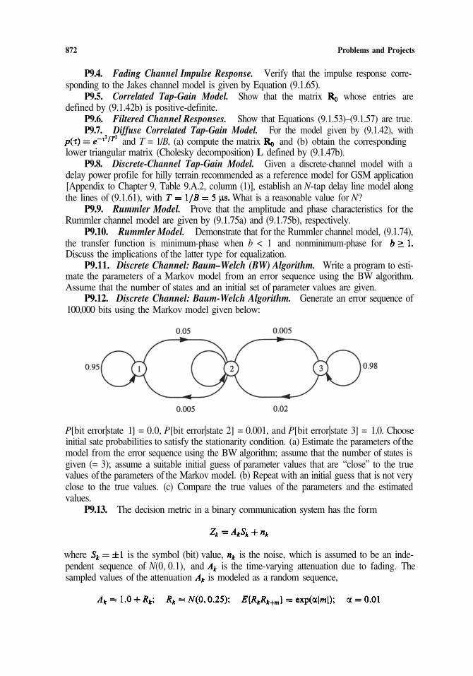
P9.12. Discrete Channel: Baum-Welch Algorithm. Generate an error sequence of100,000 bits using the Markov model given below:

P[bit error|state 1] = 0.0, P[bit error|state 2] = 0.001, and P[bit error|state 3] = 1.0. Chooseinitial sate probabilities to satisfy the stationarity condition. (a) Estimate the parameters of themodel from the error sequence using the BW algorithm; assume that the number of states isgiven (= 3); assume a suitable initial guess of parameter values that are “close” to the truevalues of the parameters of the Markov model. (b) Repeat with an initial guess that is not veryclose to the true values. (c) Compare the true values of the parameters and the estimatedvalues.

P9.13. The decision metric in a binary communication system has the form

where is the symbol (bit) value, is the noise, which is assumed to be an inde-

sampled values of the attenuation is modeled as a random sequence,

and T = 1/B, (a) compute the matrix and (b) obtain the correspondinglower triangular matrix (Cholesky decomposition) L defined by (9.1.47b).

P9.8. Discrete-Channel Tap-Gain Model. Given a discrete-channel model with adelay power profile for hilly terrain recommended as a reference model for GSM application[Appendix to Chapter 9, Table 9.A.2, column (1)], establish an N-tap delay line model along

pendent sequence of N(0, 0.1), and is the time-varying attenuation due to fading. The


(a) Outline a procedure for deriving a three-state Markov model for this case. (b) Simulate100,000 bits through this model and generate the error sequence and estimate the parametersof a three-state Markov model for this system.

Chapter 10

P10.1. Average Level Estimation. Assume a waveform has the properties of aGaussian process with average value and variance Derive an expression for a two-sidedconfidence interval for as a function of the number of sampled waveform values.

P10.2. Average Power Estimation. Show that the pdf of the average powerestimator conditioned on the signal, is noncentral gamma.

P10.3. Estimation of Distribution Function. The Kolmogorov–Smirnov (KS) test isa goodness-of-fit test for distributions (see, e.g., Ref. 5 of Chapter 10). It is used to testassumptions regarding the true distribution approximated by the empirical distribution. (a)Develop a program to apply the KS test to a sequence of “random” numbers. Use yourprogram to test your favorite random number generator (see also Chapter 7).

P10.4. Histogram Construction. Write a program that will generate a histogramfrom simulation-generated data. (Note: most commercial math analysis/simulation packageshave a built-in histogram function.)

P10.5. Histogram. Generate 100 samples of a uniformly distributed random vari-able, and compute a histogram of the 100 samples using a bin width of 0.05. (a) Plot thehistogram; does it “look” uniform? (b) Repeat for different values of the seed for the uniformRNG. (c) Repeat for a sample size of 1000.

P10.6. Estimation of Two-Dimensional pdf . Find the form of an estimator of a two-dimensional probability density function and establish its properties.

P10.7. Power Spectral Density Estimation. (a) Show that the variance of the peri-odogram does not decrease with N, i.e., that Equations (10.5.24) and (10.5.25) are true for aGaussian process. (b) Verify (a) through simulation.

P10.8. Power Spectral Density Estimation. (a) Write a program to implement asmoothed PSD estimator; incorporate at least one window. (b) Apply the estimator to asystem composed of a cascade of a source, a modulator, a filter, and a memoryless nonli-nearity. (c) Obtain and compare the PSD at the output of the modulator, the filter, and thenonlinearity.

P10.9. Power Spectral Density Estimation. Another method of reducing thevariance of a PSD estimator, aside from the Bartlett or Welch periodograms, is by smoothingin the frequency domain. The smoothed (discrete) frequency-domain estimator is

unsmoothed periodogram. (a) Show that has decreased variance, increased bias, anddecreased resolution, for a fixed number of sample points. (b) Verify (a) through simulation.

P10.10. Power Spectral Density Estimation. Generate a set of samples {X(k)},

{X(k)}. Let where a is chosen to ensure

defined as a running average, where is the

k = 0 ,1 , . . . , N – 1, of a stationary random process at a sampling rate samples/s. Estimatethe PSD of the process as follows. Let F(k), k = [–N/2], . . . , 0, . . . [N/2 – 1], be the FFT of


where and Obtain the smoothed PSD using the method of

by amplitude –1 for seconds (or samples) and “1” is represented by an amplitude of+1 for seconds (or samples). Estimate the PSD of this waveform and compare it to thatof the balanced NRZ waveform. Choose different values of the parameters; start with

P10.13. Estimation of Phase and Delay. Show that the estimates of delay and phasegiven by the cross-correlation method are identical to the maximum-likelihood estimatorswhen the system has unknown gain, delay, and phase, but is otherwise undistorted.

P10.14. Estimation of Phase and Delay. Write a program to obtain the phase anddelay of a system by using the cross-correlation technique. Implement the cross-correlationvia FFT methods. (See also Problems P7.21 and 7.22.)

P10.15. Eye Pattern/Scatter Plot. Write a program that will generate an eye pattern.(b) Write a program that will generate a scatter plot.

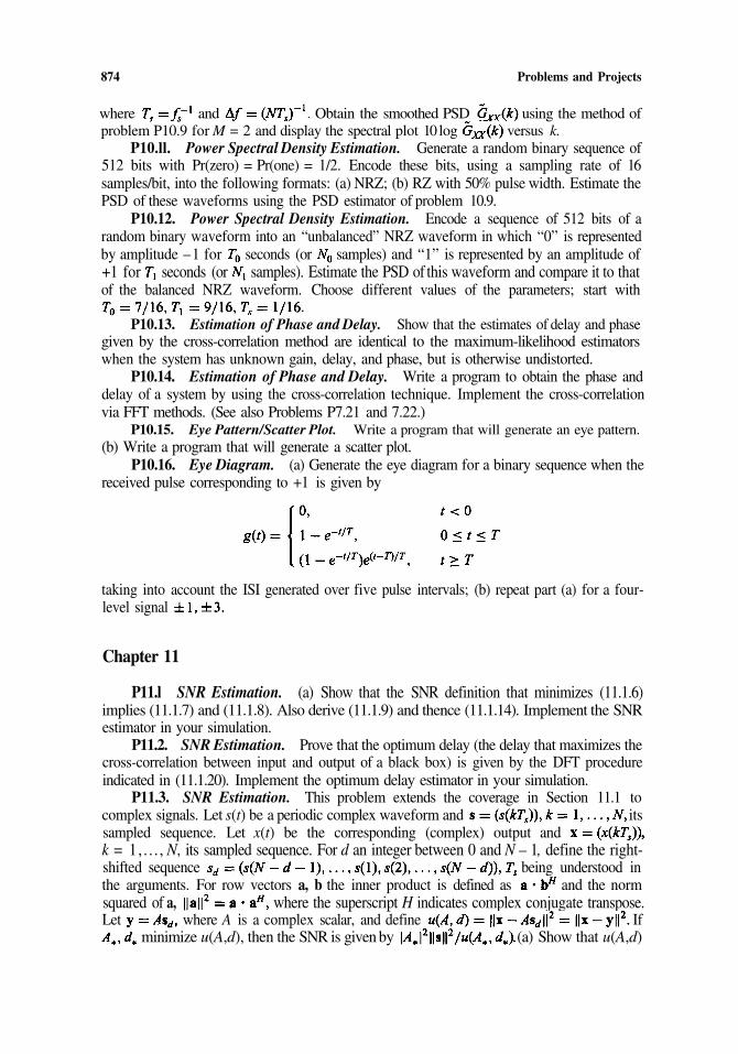
P10.16. Eye Diagram. (a) Generate the eye diagram for a binary sequence when thereceived pulse corresponding to +1 is given by

taking into account the ISI generated over five pulse intervals; (b) repeat part (a) for a four-level signal

Chapter 11

P11.l SNR Estimation. (a) Show that the SNR definition that minimizes (11.1.6)implies (11.1.7) and (11.1.8). Also derive (11.1.9) and thence (11.1.14). Implement the SNRestimator in your simulation.

P11.2. SNR Estimation. Prove that the optimum delay (the delay that maximizes thecross-correlation between input and output of a black box) is given by the DFT procedureindicated in (11.1.20). Implement the optimum delay estimator in your simulation.

P11.3. SNR Estimation. This problem extends the coverage in Section 11.1 tocomplex signals. Let s(t) be a periodic complex waveform and itssampled sequence. Let x(t) be the corresponding (complex) output andk = 1 , . . . , N, its sampled sequence. For d an integer between 0 and N – 1, define the right-shifted sequence being understood inthe arguments. For row vectors a, b the inner product is defined as and the normsquared of a, where the superscript H indicates complex conjugate transpose.Let where A is a complex scalar, and define If

minimize u(A,d), then the SNR is given by (a) Show that u(A,d)

problem P10.9 for M = 2 and display the spectral plot 10 log versus k.P10.ll. Power Spectral Density Estimation. Generate a random binary sequence of

512 bits with Pr(zero) = Pr(one) = 1/2. Encode these bits, using a sampling rate of 16samples/bit, into the following formats: (a) NRZ; (b) RZ with 50% pulse width. Estimate thePSD of these waveforms using the PSD estimator of problem 10.9.

P10.12. Power Spectral Density Estimation. Encode a sequence of 512 bits of arandom binary waveform into an “unbalanced” NRZ waveform in which “0” is represented


is minimized by the choice of A and d that maximize (b) Show that this isequivalent to choosing the A and d that maximize (c) Show that

P11.4. The Monte Carlo Method for Evaluating Integrals. We have seen [e.g., in(11.2.1)] that estimating the BER is equivalent to evaluating an integral. Typically we do notknow the integrand, and in the MC method we evaluate the integral by observing its randomlygenerated values. The MC method can also be used to evaluate integrals with known inte-grands that might otherwise be difficult to solve. To illustrate the method, evaluate by MCmeans the integral

Use several sets of random numbers with different sizes (e.g., 100, 1000) and compare to thetrue value. Hint: Write I as an expectation.

P11.5. Constructing a Monte Carlo BER Curve. (a) Devise a smooth interpolationroutine to “best-fit” a BER curve from a set of Monte Carlo estimates at different values of

take into account the relative reliability of these different estimates. (b) Apply theresults of part (a) to an actual simulation.

P11.6. Confidence Interval for BER. (a) Formulate a one-sided confidence intervalfor BER based on the binomial distribution and on the normal approximation. (b) Obtain theone-sided confidence intervals for 90%, 95%, and 99% confidence levels. (c) Discuss theimplications of two-sided versus one-sided confidence intervals for the BER.

P11.7. BER Estimation for a Symbol with a Random Number of Occurrences.Consider the MC BER estimator (11.2.3) for a particular symbol when the total number ofsuch transmitted symbols is random. (a) Show that this estimator is unbiased. (b) Show thatthe estimator variance is given by (11.2.24).

P11.8. Dependent Errors. Starting with (11.2.27), show that (11.2.28) is true.P11.9. Sequential Estimation for BER. Derive Equation (11.2.32a).P11.10. Tail Extrapolation. (a) Derive the form of the tail extrapolation estimator,

(11.2.46) and (11.2.47). (b) Quantify the error term as a function of the exponentparameter (c) Show that the best-fit tail extrapolation estimator with three equally spacedpseudothresholds (in decibel domain) is given by (11.2.50). (d) Write a program to implementthe tail extrapolation estimator.

P11.11. Bias of the IS Estimator. (a) Show that the IS estimator (11.2.58) for theoutput version is unbiased. (b) Show that the IS estimator for the input version (11.2.65) isunbiased if no impulse response truncation takes place. (c) Show that if impulse responsetruncation occurs, there must be some estimator bias.

P11.12. Variance of the IS Estimator. (a). Obtain the variance of the BER estimator(11.2.59) for the input version of IS. (b) Obtain the variance of the BER estimator (11.2.70)for the output version of IS.

P11.13. Conditional Importance Sampling. The form of IS conditioned on simu-lating only a relatively few (worst) ISI patterns requires the identification of those patterns.For a linear system, suppose you had the response p(t) coresponding to a 1; set up a recursivecomputation to rank the ISI patterns.

P11.14. Variance of the CIS and IIS Estimators. Derive Equations (11.2.73a) and(11.2.73b) in Example 11.2.5.


P11.15. Optimum Value of Bias for CIS. Suppose we want to estimateusing conventional importance sampling. Derive an expression for

variance of the estimator as a function of T and sample size N. Find the optimum value of thebias, i.e., the factor by which the variance should be increased.

P11.16. CIS with Memory. Find the optimum biasing for in order to evaluatewith Compare the variance reduction possible to that in

Problem P11.15.P11.17. Comparing Different Estimation Methods. Consider a binary commu-

nication system in which a random binary source (± 1 V) sampled at 8 samples/bit is addedto a noise source and the sum input to a detection filter with impulse response

where is the bit duration. The output is sampled at multiples of in order to make adecision. Estimate the probability of error using the following techniques. (a) An analytical(exact) expression; (b) Monte Carlo, with bits; (c) quasianalytical, with 100 random bits;(d) conventional importance sampling with 10 random bits; (e) improved importancesampling with 10 random bits. Compare the estimated values to one another. Repeat thesimulations 10 times and estimate the bias and variance of the estimators.

P11.18. QA Method for PAM. Derive equations for use in QA simulation that givethe specific error rates for PAM (Section 11.2.7.3). The specific error rate is the probability ofdeciding on a particular symbol other than the transmitted one

P11.19. QA Method for QAM. Derive an equation for QA application for the errorrate of symbols on the periphery of a QAM rectangular constellation.

P11.20. QA Method for PSK. Show that Equation (11.2.101) is true. Bound theerror analytically, and estimate the computational requirement for the bound relative to theexact result (11.2.99).

P11.21. QA Method with ISI. Consider a binary system with received waveformcontaining ISI and additive Gaussian noise

with (a) Show that the average BER is given by

where is the variance of the noise. (b) For SNR varying from 5 to 20 dB, estimate p bysimulation when the number of ISI terms is equal to eight (four on either side of for thepulse

(c) Repeat part (b) with 12 ISI terms.P11.22. QA Method with Interference. The average error rate of a binary PSK

signal corrupted by additive Gaussian noise and cochannel interference


uniformly distributed on is given by

where is the variance of the noise. Evaluate this expression by simulation for variousvalues of SNR, and plot the running simulation average, versus N, the current number ofgenerated values of Observe the rate at which tends to the “true” value [for the latter,see, e.g., V. K. Prabhu, Error rate considerations for coherent phase-shift-keyed systems withco-channel interference, Bell Syst. Tech. J. 48(3), 1304–1310 (1969)].

P11.23. Error Probability Estimation by Statistical Averaging Method. Write aprogram to determine the BER via the method of averaging a QA estimate (obtained withoutphase and timing jitter) over a distribution of phase and timing errors (the technique discussedin Section 11.2.7.8).

P11.24. QA Method for BER Evaluation of a System. Consider a system whichconsists of the following cascade of elements: A transmit filter (six-pole Butterworth withBT = 1.0); a nonlinear amplifier with characteristics given as follows (BO = backoff):

an additive noise source with PSD and a receive filter (four-pole Butterworth), withvariable BT. (a) For an MPSK signal (try a couple values of M), plot BER as a function ofreceiver BT in the range 0.5,...., 1.2, for different values of Find the optimumreceiver bandwidth, and plot BER versus for the optimized filter. How different is theoptimum bandwidth for different (b) Now input a 16-QAM signal, but fix the receiveBT at 0.7. Run simulations for 0, –3, –6, –9 dB input backoff. For a given atsaturation, plot the BER as a function of backoff and determine the optimum backoff forseveral values of

P11.25. QA Method with Coding. Obtain an expression for the error magnificationin the BER estimate using the transfer function bound, if the channel transition probabilities

are obtained from MC simulation.

I where and are the respective modulations, and is taken to be

Appendix A

A Collection of Useful Resultsfor the Error Probabilityof Digital Systems

It is a standard part of methodology to check the results of a simulation by comparing them tocertain known benchmarks. This is useful both for debugging and validation purposes. In thefirst instance, of course, we set up the simulation so that it should yield the known results.These known results typically apply to theoretical models that are idealizations of realsystems. Therefore, strictly speaking, they cannot “validate” a simulation of a real system,but they do provide a “sanity check” in the sense that they serve as lower bounds on the (errorprobability) performance of real digital systems. Furthermore, if the simulated results differfrom the theoretical results by an amount that seems excessive, that may be symptomatic ofinadequate models. Therefore, as an aid to this checking process, we present in this Appendixa short collection of known formulas, approximations, bounds, and curves for the errorprobability for a variety of digital communication systems.

The general setting for these known results is as follows. During a signaling interval, the

where is the complex equivalent lowpass waveform (for practical purposes, the same asthe complex envelope). Each waveform (symbol) is characterized by an energy per symbol

and related to other waveforms by a cross-correlation coefficient

879

transmitter selects one of M waveforms m = 1 ,2, . . . , M, which can be represented inthe form

880 Appendix A

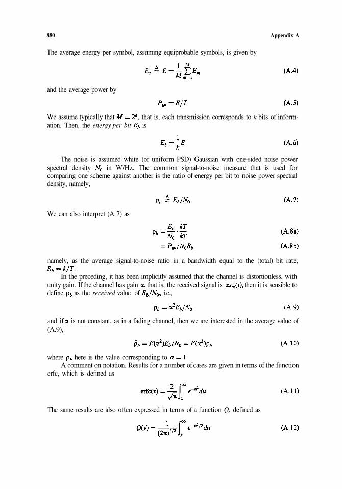
The average energy per symbol, assuming equiprobable symbols, is given by

and the average power by

We assume typically that that is, each transmission corresponds to k bits of inform-ation. Then, the energy per bit is

The noise is assumed white (or uniform PSD) Gaussian with one-sided noise powerspectral density in W/Hz. The common signal-to-noise measure that is used forcomparing one scheme against another is the ratio of energy per bit to noise power spectraldensity, namely,

We can also interpret (A. 7) as

namely, as the average signal-to-noise ratio in a bandwidth equal to the (total) bit rate,

In the preceding, it has been implicitly assumed that the channel is distortionless, withunity gain. If the channel has gain that is, the received signal is then it is sensible todefine as the received value of i.e.,

and if is not constant, as in a fading channel, then we are interested in the average value of(A.9),

where here is the value corresponding toA comment on notation. Results for a number ofcases are given in terms of the function

erfc, which is defined as

The same results are also often expressed in terms of a function Q, defined as

Error Probability of Digital Systems 881

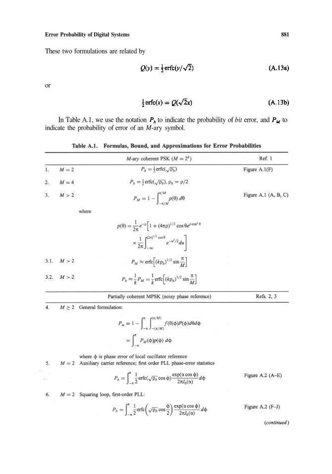
These two formulations are related by

or

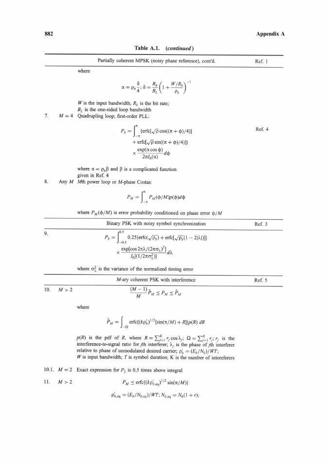
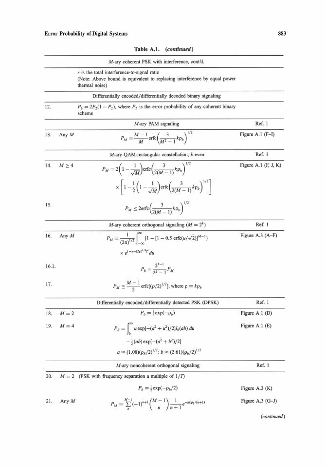
In Table A.1, we use the notation to indicate the probability of bit error, and toindicate the probability of error of an M-ary symbol.

882 Appendix A


884 Appendix A


886 Appendix A

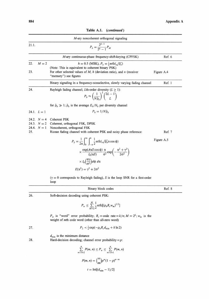
Figure A.1. Bit and symbol error probabilities forvarious coherent modulation schemes. A, 8-PSK:B, 16-PSK: C, 32-PSK: D, 2-DPSK: E, 4-DPSK: F, 2-PSK, 4-PSK, 4-QAM, 2-PAM: G,4-PAM: ; H, 8-PAM: I, 16-PAM: J, 16-QAM: K, 64-QAM: L–N, Rate-1/2 convolu-tional codes; code parameters Viterbi decod-ing; PSK modulation; L, L = 9, M,L = 7, N, L = 5,

Figure A.2. Effect of phase noise on binary PSK errorprobability. A–E, Auxiliary carrier: A, LoopSNR = 3dB; B, loop SNR = 7dB; C, loopSNR=10dB; D, loop SNR=15dB; E, loopSNR = 20 dB. F–J, Squaring loop; F, G,


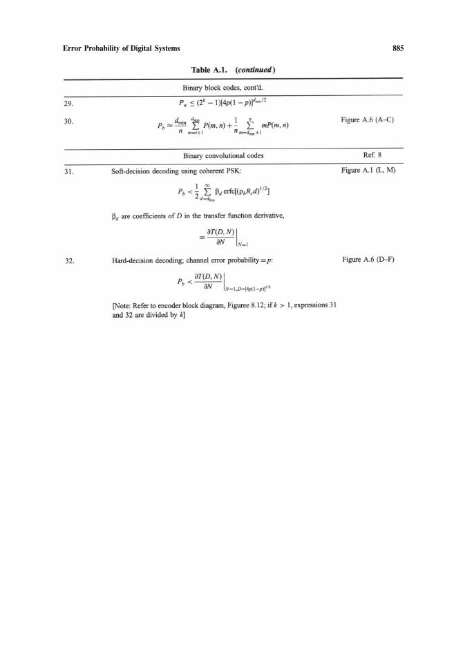
Figure A.3. Bit error probability for coherent andnoncoherent M-ary orthogonal signaling. A–F, Coher-ent detection: A, M=64: B, M=32: C,

G–K, Noncoherent detection: G, M = 32: H,

detection: A, 2-CPFSK, h = 0.715, n = 2: B, 2-CPFSK, h = 0.715, n = 3: C, 2-CPFSK, h = 0.715,n = 4: D, 4-CPFSK, h=1.75, n = 2: E, 4-CPFSK,

CPFSK, h = 0.879, n = 3: H–K, Noncoherent detec-tion: H, 2-CPFSK, h = 0.715, n = 3: I, 2-CPFSK,

4-CPFSK, h = 0.8, n = 5:

M=16: I, M=8: J, M=4: K, M=2:

Figure A.4. Bit and symbol error probabilities forcontinuous phase frequency-shift-keying (CPFSK) forcoherent and noncoherent detection. A–G, Coherent

M=16: D, M=8: E, M=4: F, M=2:

h = 0.8, h = 3: F, 8-CPFSK, h = 0.879, n = 2: G,8-

h = 0.715, n = 5: J, 4-CPFSK, h = 0.8, n = 3: K,

888 Appendix A

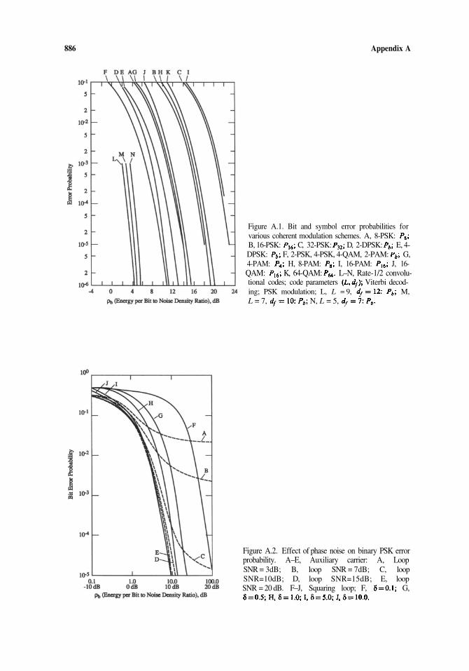
Figure A.5. Bit error probability for slow-fading Ricean channel with noisy phase reference. Reference loopSNR=15dB: is ratio of specular to diffuse energy.


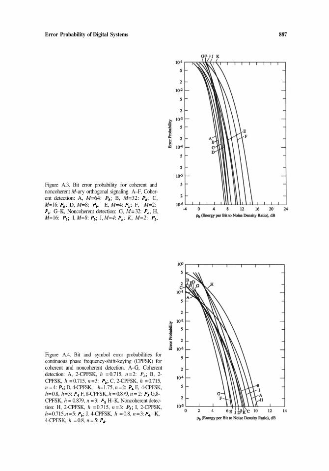
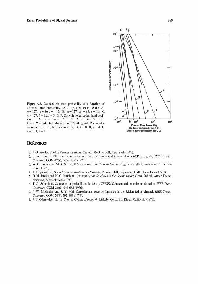
Figure A.6. Decoded bit error probability as a function ofchannel error probability. A–C, (n, k, t) BCH. code: A,n = 127, k = 36, t = 15; B, n = 127, k = 64, t = 10; C,n = 127, k = 92, t = 5. D–F, Convolutional codes, hard deci-sion: D, L = 7, R = 1/3; E, L = 7, R–1/2. F,L = 9, R = 3/4. G–J, Modulation; 32-orthogonal, Reed–Solo-mon code: n = 31, t-error correcting. G, t = 8. H, t = 4. I,t = 2. J, t = 1.

References

1.2.

3.

4.5.

6.

7.

8.

J. G. Proakis, Digital Communications, 2nd ed., McGraw-Hill, New York (1989).S. A. Rhodes, Effect of noisy phase reference on coherent detection of offset-QPSK signals, IEEE Trans.Commun. COM-22(8), 1046–1055 (1974).W. C. Lindsey and M. K. Simon, Telecommunication Systems Engineering, Prentice-Hall, Englewood Cliffs, NewJersey (1973).J. J. Spilker, Jr., Digital Communications by Satellite, Prentice-Hall, Englewood Cliffs, New Jersey (1977).D. M. Jansky and M. C. Jeruchim, Communication Satellites in the Geostationary Orbit, 2nd ed., Artech House,Norwood, Massachusetts (1987).T. A. Schonhoff, Symbol error probabilities for M-ary CPFSK: Coherent and noncoherent detection, IEEE Trans.Commun. COM-24(6), 644–652 (1976).J. W. Modestino and S. Y. Mui, Convolutional code performance in the Rician fading channel, IEEE Trans.Commun. COM-24(6), 592–606 (1976).J. P. Odenwalder, Error Control Coding Handbook, Linkabit Corp., San Diego, California (1976).

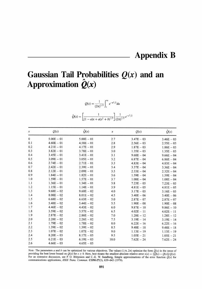
Appendix B

Gaussian Tail Probabilities Q(x) and anApproximation

891

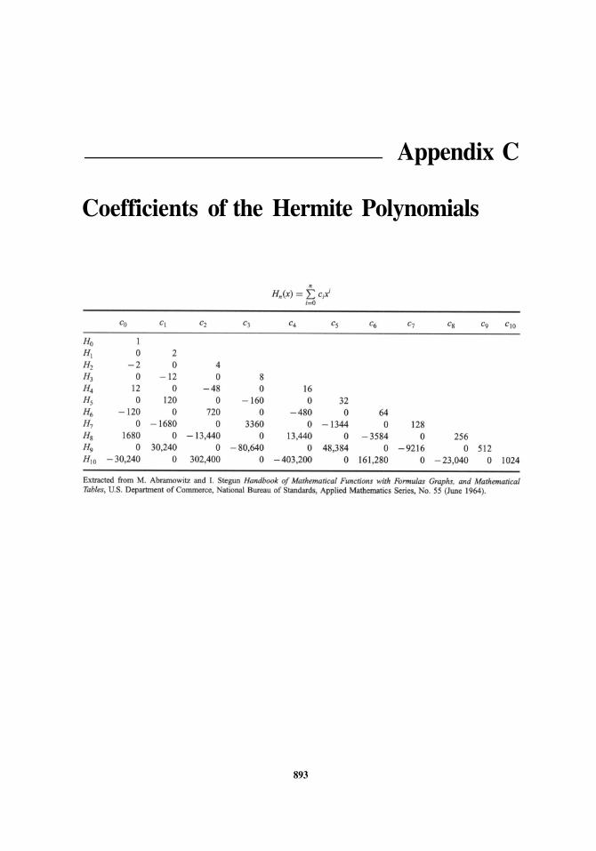
Appendix C

Coefficients of the Hermite Polynomials

893

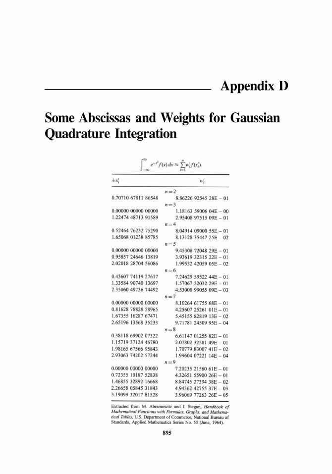
Appendix D

Some Abscissas and Weights for GaussianQuadrature Integration

895

Appendix E

Chi-Square Probabilities

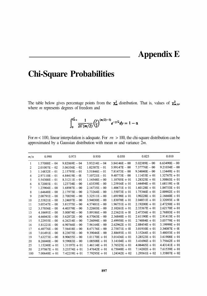
The table below gives percentage points from the distribution. That is, values ofwhere m represents degrees of freedom and

For m < 100, linear interpolation is adequate. For rn > 100, the chi-square distribution can beapproximated by a Gaussian distribution with mean m and variance 2m.

897

Index

Acceptance-rejection method, 381–383Adjacent channel interference (ACI), 406Algebra of LTV Systems, 135Aliasing, 87; see also SamplingAutocorrelation function

properties, 329, 335of stationary processes, 335

Autoregressive moving average modelsARMA model, definition, 342

applied, in Case Study II, 804AR model, 343MA model, 343

autocorrelation, 343parameter estimation, 349

Yule–Walker equations, 349power spectral density, 343, 804vector ARMA model, 399

Baseband modulation, 417–425differential encoding, 420line coding, 420–425partial response signaling, 425

BERestimation of, 678–757

conceptual framework, 683–686importance sampling, 710–734interval measures, 697–703mixed quasianalytical, 754–757moment method, 787–790Monte Carlo, 686–703quasianalytical, 737–754run-time implications, 679–683tail extrapolation, 703–710

evaluation ofblock-coded systems, 748–753convolutionally coded systems, 749–750, 753formulas for, 881–885

Bias, see also Expected value of estimatorsasymptotic, in tail extrapolation, 707statistical, 628

Biased density, 711–712, 715

Bilinear transformation, 173–178frequency pre warping, 176–177, 179frequency warping, 176

Biquadratic sectionscontinuous, 112–113

canonic form, 113discrete, 166

cascade interconnection, 168parallel interconnection, 169

Bounds, see also InequalitiesChebychev, 317Chernoff, 318union, 318

Calibration of simulations, 534–539Carrier recovery

for BPSK, 504–506Costas loop, 507, 527–528effect on BER, 753–754estimation of phase, 655–661

block processing, 660–661cross-correlation, 655–657

lowpass equivalent, 507, 512Mth power loop, 511–512PLL, 495–534

phase error distribution, 662–664for QPSK, 510–512simulation, 495, et seq.squaring loop, 506

CDMA, see also Multiplexing/multiple accessapplied, in Case Study IV, 822–848

Central limit theorem, 320Channel capacity

AWGN, 425discrete memoryless, 426

Channel (fading) simulation methodology: see Simula-tion methodology

Channels, channel models: see Finite-state channelmodels; Free-space channels; Guided mediachannels; Multipath fading channels

899

900 Index

Cochannel interference (CCI), in Case Study IV, 829–831

Coded modulation, 449–451block-coded modulation, 449–450trellis-coded modulation, 450–451

Coded systems, see also Error control codinghard decision,

with dependent errors, 751–753with independent errors, 748–751

quasianalytic simulation of, 748–753soft decision, 753

Communication system, generic block, diagram, 408Confidence interval

for average level, 635–636for BER, based on

binomial distribution, 688–691normal distribution, 691–694Poisson distribution, 498–500

defined, 629–631Convolution property, 68–69Convolution property for periodic signals, 73Convolution theorem

applied to filtering, 135convolution sum, 63

Correlated Gaussian sequencesgeneration of spatially correlated Gaussian

sequencesCholesky method, 388–399covariance factorization method, 398

generation of temporally correlated Gaussiansequences

ARMA models, 394FIR method, 397spectral factorization method, 396

spatial correlation, 394temporal correlation, 394

Correlation coefficient, 295Correlogram, 646–647Covariance

matrix, 296scalar, 295

Cross-correlationfor estimating delay, 655–656for estimating SNR, 671–673

Cross-correlation functionproperties, 336of stationary processes, 335–336

Cross PSDdefinition, 338properties, 338–339

Delayeffect on phase-locked loop, 524, 531–534estimation of, 655–657, 658–659in SNR estimation, 675–678

Demodulation/demodulatorsanalog

coherent, 457–460discriminator, 461–465

Demodulation/demodulators (cont.)analog (cont.)

envelope demodulator, 461noncoherent, 460–466PLL, 465–466square-law demodulator, 461

digitalcoherent, 457–460noncoherent, 460–466quadrature form, 457–458

Dependent errors, 696–697, 751–753Difference equation, 165; see also ARMA modelsDifferential equations

linear time-invariant (LTI), 110transfer function, 111

linear time-varying (LTV), 192–193impulse response, 192

nonlinear: see Nonlinear differential equationsDifferentiation, discrete-time, 462–465Discrete Fourier transform (DFT), 119Discrete (Markov) channel models: see Finite-state

channel modelsDiscrete (sampling) model for LTV systems, 195–196Discrete-time systems: see SystemsDistribution: see Random variables

Empirical distribution, 640–641Equalizers, 474–481

applied, in Case Study I, 773–776fractionally spaced, 475LMS algorithm, 478simulation, 480–481synchronous, 475TDL structure, 474weight calculation, 476–480

by covariance inversion, 479–480gradient algorithm, 476–477

Error control codingbandwidth expansion, 750block coding/decoding, 428–431

computational load, 430block error distribution

based on gap distribution, 700for a Gilbert channel, 751–753

code performancebinary block code, 749Reed–Solomon, 749

code rate, 428, 431coding gain, 751convolutional coding/decoding, 431–433

computational load, 432interleaving

in Case Study II, 794word error probability, 700

quasianalytical method, applied to, 748–753Reed–Solomon code, 428, 749simulation of, 427, 748–753Viterbi algorithm, 431–432

Error indicator function, 687

Index 901

Error probability: see BER; Estimation of BEREstimation (of)

average level, 631–635average power, 636–640bit-error-rate (BER), 678–757carrier phase: see Carrier recoveryerror-free intervals, 697–703power spectral density, 645–654probability density function, 640–641probability distribution function, 641–645signal-to-noise ratio, 670–678symbol timing: see Timing recovery

Estimatorbias of, 628consistent, 628variance of, 629

Expected value of estimator (of)average level, 632average power, 637BER (importance sampling), 718BER (Monte Carlo), 694power spectral density, 651–652probability density, 653–654

Expected valuesapproximate computation, 321–323conditional, 295covariance

matrix, 296scalar, 295

mean, 293, 296standard deviation, 293variance, 293

Eye diagram, 664–666applied, in Case Study I, 780

Fading: see Multipath fading channelsFast Fourier transform (FFT), 120–121F distribution, 304

in SNR estimation, 694Feedback loops, 47; see also Phase-locked loops

simulation of, 47Filters, see also FIR filters; IIR filters

adaptive, 474–481biquadratic decomposition, 112–113, 166classical filters, 136–141

Bessel, 140Butterworth, 137Chebyshev, 138–139elliptic, 139frequency transformations, 141lowpass equivalent, 142–144

Doppler: see Multipath fading channelsFIR filters: see Finite impulse response (FIR) fil-

tersfunctional filters, 481–482

amplitude ripple, 481amplitude tilt, 482cubic phase, 482

Filters (cont.)functional filters (cont.)

parabolic gain, 482parabo lic phase, 482

ideal filters, 136bandpass, 136bandstop, 136high-pass, 136low-pass, 136

IIR filters: see Infinite impulse response filtersmatched, 472–473minimum MSE, 470

Wiener filter, 470noise bandwidth

computation, 662definition, 262

pole-zero, 143lowpass equivalent, 143

preemphasis/deemphasis, 348pulse shaping, 468–469; see also FIR filtersquadrature, 77raised cosine, 468

in Case Study I, 767–768recursive: see Infinite impulse responsesimulation (of)

FIR filters, 149–165IIR filters, 165–181summary, 182–184

spectral shaping, 467square root, 469, 472

in Case Study I, 767–768tabular filters, 483–484

Finite impulse response (FIR) filters, 147, 149–165with DFT, 154–158

block processing, 159example, 161–162for nonperiodic signals, 101–107overlap-and-add, 155–156overlap-and-save, 156–158

time domain, 149–151windowing, 150–151

Finite-state channel models, 596–609applied, in CDMA example (Case Study IV), 838Baum–Welch algorithm, 606

backward recursion, 608forward recursion, 606

definition, 596–597examples

binary symmetric, 598HMM, 602M-ary, 598soft-decision, 598

Fritchman model, 604Gilbert model, 604HMM: (hidden Markov model), 600

modified, 608interval (error-free) simulation: see Estimation of er-

ror-free intervalsinterval simulation, 388

902 Index

Finite-state channel models (cont.)model types

with memory, 599memoryless, hard-decision, 598memoryless, soft decision, 598

parameter estimation, 606;Baum–Welch algorithm, 606

Formatting/source coding, 414–417A/D conversion, 414quantization, 415–416

Fourier analysiscontinuous, 66–74discrete, 118–126

Fourier series, 65Fourier transform, 66–67

for periodic signals, 72properties, 67–70table of, 129

Fourier transform for periodic signals, 35, 96Free-space (almost) channels, 586–591

absorption, 587ionospheric effects, 589rain attenuation, 587–588tropospheric effects, 587

Frequency domain representationlinear time-invariant (LTI), 63–74, 119–126linear time-varying (LTV), 188–189

Frequency responsediscrete, 124Fourier transform, 70Laplace transform, 114z transform, 124

Galois field, 390Gaussian distribution

approximation, 301table (of Q function), 891

Gaussian quadratureapplied, in Case Study I, 787–790

Gaussian random processbandpass, 354–357

envelope, 356lowpass equivalent, 354–355phase, 356quadrature model, 354

definition, 351–352ergodicity, 333stationarity, 352white PSD, 352–353

autocorrelation, 352bandlimited, 353

Generalized exponential distribution, 304applied to BER estimation, 703, 741, 743–744

Generation of random sequencescorrelated sequences, 392PN sequences, 386–390sampled white noise, 383, 385uncorrelated sequences, 384

Gibbs (the) phenomenon, 71, 150

Gilbert model, 246, 392Glivenko’s theorem, 641Guided media channels, 591–595

optical fibers, 593waveguides, 591

Hilbert transform, 75–77properties, 77–78

Histogram, 641–642

Importance sampling, 710–734biasing, 719–721, 724–732conventional, 720implementation considerations, 713–717, 732–

734improved, 721variance, 718

Importance splitting, 734–737Impulse-invariant transformation, 170–173, 178

aliasing, 170for rational functions, 171

Impulse responsecontinuous, 62discrete, 62

Incomplete gamma function, 741Inequalities, 317–319

Chebychev, 317Chernoff, 318

Infinite impulse response (IIR) filters, 165–181, 184classical, continuous, 136–141

lowpass equivalent, 142–144impulse-invariantmapping from continuous to discrete: see Bilinear;pole-zero (example of), 172realization using biquadratic expansion, 79

continuous, 112–113, 80discrete, 166–169

Information sourcesanalog signals, 411–413

filtered random processes, 413multiple tones, 412single tone, 412

binary PN sequences, 386digital signals, 413–414M-ary PN sequences, 390

Interconnection of systemscascade connection of biquadratic sections

continuous, 112discrete, 168

in frequency domain, 70of LTI systems, 108–110of LTV systems, 190–192parallel connection of biquadratic sections

continuous, 112discrete, 166–169

Interferencein Case Study IV, 829–831in CDMA, 490in FDMA, 490

Index 903

Interleavingapplied, in Case Study II, 794

Interpolation, 89–105bandlimited, 86, 96–98cubic spline, 100–105linear, 49, 98–100in multirate application, 88–89, 93–96

Laplace transform, 106–107properties, 107–108table of, 130

Large-deviations theory, 724–732Linear time-invariant (LTI) systems, see also Filters;

FIR filters; IIR filterscontinuous, 62, 70, 110–115discrete, 62, 115–118

Linear time-invariant (LTI) systems: discrete, 22, 72–124

convolution sum, 22impulse response, 22

Linear time-varying (LTV) systems, 184–196impulse response, 186–187properties of, 190–192superposition integral, 187

Line coding, 420–425biphase, 423correlative, 421delay, 423differential, 420Miller, 421NRZ, 422–423partial response, 425RZ, 423spectral shaping, 424

Lowpass equivalents, 74–83applied to filtering, 81–82bandpass filter, 79–81bandpass nonlinearity, 219–220classical filters, 142–144complex envelope, 75modeling, 82–83modulated signal, 78–79preenvelope (analytic signal), 77of random signals, 362–366in system analysis, 79–82

Mapping from continuous to discrete: see Bilineartransformation; Impulse-invarianttransformation

Methodology, see also Simulation methodologyapplied, chapter 12

Mixed quasianalytical method, 754–757Mobile radio channels: see Multipath fading chan-

nelsModeling

concepts of, 17–26errors in, 28–36

Modulation/modulators,433–457analog

AM, 433–434327FM, 434PM, 434quadrature, 434–435

digitalASK, 438coded modulation, 449–451CPFSK, 445–446CPM, 443–449general quadrature, 435–438modeling considerations, 451–455MSK, 446–447OFDM, 439–442OQPSK, 438Pi/4 QPSK, 438–439PSK, 438QAM, 438

applied, in Case Study I, 766signal constellation, 437

Moment method, 322applied to BER evaluation,

in Case Study I, 787–790Moments

of finite sums, 322–323recursive computation, 323

in Case Study I, 787–790Monte Carlo simulation, definition, 15, 316, 371–373

applied to BER estimation, 686–703variations, 26–27, 373

modified MC, 373pure MC, 371

Multipath fading channels, 546–586delay

rms, 557spread, 556

diffuse multipath model, 561–572Cholesky factorization, 567example, with correlated tap gains 570filtered delay-power profile, 568separable scattering function, 565tapped delay-line models, 563–565

discrete multipath model, 572–575example, with filtered model, 572filtered discrete model, 572

Dopplerfast fading, 560, 561Jakes autocorrelation function, 558Jakes spectrum, 558slow fading, 560, 561Spread, 560

fadingcoherence BW, 557coherence time, 560frequency non-selective (flat), 554, 558frequency selective, 554, 558

fading, large scale (shadow)lognormal shadowing, 549

904 Index

Multipath fading channels (cont.)fading, small scale (multipath)

delay power profile, 554Doppler spectrum, 554random process model, 553–554Rayleigh, 552Rician, 552

indoor wireless channel models, 576–583factory and open plan building, 577office building, 578ray-tracing, 547, 582

line-of-sight (LOS) radio channel modelLOS radio Case Study, 769–793minimum-phase, 585non-minimum phase, 586Rummler model, 583–584

lowpass equivalent, 550–551path loss measurements, 549path loss (shadowing) models, 548

COST-231 model, 548Hata model, 548ray-tracing, 547, 582

propagation effects, 546reference models for GSM applications, 614

Doppler spectrum types, 616hilly terrain, 615rural areas, 614urban areas, 615

reference models for PCS applications, 617reference models for UMTS-IMT-2000 applications,

618decorrelation length, 619impulse response (delay spread), 619indoor, 618outdoor to indoor and pedestrian, 618vehicular, 618

scattering function, 554simulation of, 561–576

LOS radio, 783, 785spaced-frequency correlation function, 557spaced time correlation function, 558statistical characterization, 551–554tap-gain models

correlated, 565–567generation of tap-gain processes, 575–576multirate, 845–846uncorrelated, 564

tapped delay-line modelsfor diffuse channels, 563for discrete channels, non-uniformly spaced, 572for discrete channels, uniformly spaced, 573

wideband channel measurements, 561WSSUS model, 553

Multiplexing/multiple access, 484–491CDMA, 489–491FDMA, 486–487PDMA, 484–485SDMA, 484–485TDMA, 487

Multirate processing, 83, 87–89, 91–96Multivariate Gaussian, 305–308

conditional, 306joint, 305linear transformation, 306marginal, 306moments, 308properties, 306

Noiseband-limited, 352Gaussian, 350–356impulse noise, 348–350quadrature representation, 354–356shot noise, 346–348thermal noise, 352white, 352

Nonlinear differential equations, 257–275applied to optical amplifier, 271–275integration formulas, 261–262

explicit, 263implicit, 263–266stability, 267, 269–270truncation error, 268–269

Nonlinear systems, 203–256analytic bandpass memoryless models

Chebyshev transform, 210describing function, 210limiters, 213power series, 214

analytic models with memory, 237–252polyspectral models, 245–252Volterra series, 237–245

baseband modelsgeneral, 206–207hysteresis, 211limiter, 212–213

block models, memoryless, 215–223AM/AM, AM/PM, 215, 218–219, 220–221lowpass equivalent, 219–220quadrature model, 217serial model, 216

block models with memory, 227–237Abuelma’atti model, 232–234instantaneous frequency model, 255nonlinear parametric model, 253power-dependent transfer function model, 252Poza–Sarkozy–Berger model, 227–229Saleh’s model, 154three-box models, 236–237two-box models, 234–236

intermodulation products, 221–223measurement techniques, 275–284

time-domain, 280–284two-tone, 278–280VNA, 275–277

nonlinearities with memory, classification, 224–227

sampling rate, 207–209

Index 905

Optical amplifier model, 271–275Optical fiber model

multimode, 370–373single mode, 370–373

Optical source models, 492–494rate equations, 492simulation model, 493–494

block diagram, 493explicit form, 494

Order of computation, 524Order of execution, 524Order statistics, 315Outage probability

definition, 790–791estimation methodology

example in Case Study I, 781–793Overlap-and-add: see Finite impulse response (FIR)Overlap-and-save: see Finite impulse response (FIR)

Parseval’s theoremapplied to SNR estimation, 687for continuous signals, 32for discrete signals, 95for periodic signals, 26

Periodogram, 647–648Phase-locked loop

assembled model, 522–529effect of delay on, 531–534

distribution of phase error, 662–663as an FM demodulator, 465–466, 529–531modeling considerations, 514–515stand-alone model, 515–522

Phase noiseARMA model for residual, 804averaging effects of, on BER, 753–754distribution, in a PLL, 662–663equivalent process methodology, 502–504

general model for, 800residual, 799–803

effect on block-coded systems, Case Study II, 808tracked, 800untracked, 800

variance, of phase error, 663Poisson Process, 346Power spectral density (PSD), 336–340

bandpass, 337bandwidth, 337definition, 336estimation of, 645–654lowpass, 337power calculation, 337properties, 336of random sequences, 339

Probability density function (pdf)conditional, 295definition, 293estimation of, 645–654joint, 294marginal, 294

Probability distribution function, 293estimation of, 640–641

Probability mass function, 293Pseudo-BER, 705Pseudonoise (PN) sequences, 386–392

binary, 386–389generation, 386–388, 389

octal, 391properties, 387–389quaternary, 392

Pseudothreshold, 705

Quadrature ruleformula, 323–324weights for Gaussian, 895

Quantization, 415–416of a Gaussian pdf, 369A-law, 416MSE, 367,369mu-law, 415nonuniform, 368–369about simulating, 416–417uniform, 367–368

Quasianalytical (QA) method, 737–754applied to binary systems, 740–743applied to hard-decision-decoding, 748–753applied to PAM systems, 743–744applied to PSK systems, 745–748applied to QAM systems, 744–745applied to soft-decision decoding, 753–754fast QA, applied to Case Study I, 786–787incorporating jitter, 753–754

Quasistatic approach to simulation, 570, 653

Radio channels: see Multipath fading channelsRadio-relay system, Case Study I, 763–793Random number generators (RNG)

arbitrary pdf, 377acceptance/rejection method, 381–382transformation method, 377

exponential, 379gamma, 379Gaussian, 383–384

Box-Muller method, 383correlated sequences, 392summation method, 383white noise, 383

geometric, 379Poisson, 379seed, 374,387summary of algorithms, 384uniform RNG, algorithms for 374–37

linear congruential, 374Marsaglia–Zaman, 376–377Wichman-Hill, 376

Random processesclassification, 326–327

continuous amplitude, 326–327continuous time, 326–327

906 Index

Random processes (cont.)classification (cont.)

discrete amplitude, 326–327discrete time, 326–327

complex-valued, 326–327definitions, 326–327ensemble averages, 329–331

autocorrelation, 329autocovariance, 329correlation coefficient, 330ergodicity, 331mean, 329

member function, 326notations, 326simulation implications, 333stationary, 331

strict sense, 331wide sense, 331

time averages, 332transformation, 357

Random sequencesARMA model, 342

applied to residual phase noise, 804autoregressive (AR), 342binary PN, 386independent, 340Markov 340M-ary PN, 389moving average (MA), 342PSD of, 339, 343random binary, 345random M-ary, 344white, 340

Random variablescomplex-valued, 297continuous, 293

chi-square, 303exponential, 301F, 304gamma, 302Gaussian, 301,304generalized exponential, 304Rayleigh, 302Rice, 356student’s t, 303uniform, 300

definition, 292discrete, 293

binomial, 298Erlang, 302geometric, 299multinomial, 304negative binomial, 299Poisson, 299uniform, 298

real-valued, 292scalar (univariate), 294vector (multivariate), 294

RF sources, 491–492phase noise, 491

Roundoff noiseFFT, 182FIR filters, 182IIR filters, 181

Samplingof deterministic signals

impulse sampling, 83–85sampling rate for nonlinear systems, 207–208sampling theorem, 86

of random processes, 363–367aliasing, 364aliasing error, 365bandpass, 365lowpass, 363–364minimum rate, 363–364reconstruction, 363sampling principle, 363–364

Sampling rate, for simulation, 365; see also MultirateScatter diagram, 666–667

applied, in Case Study III, 815–817, 819, 821–822

Semianalylic: see Quasianalytical

Separable model for LTV 132Shot noise, 251–252Signals, 14–56–59

continuous, 56–57discrete, 57–59periodic, 72

Signal-to-noise ratio estimation, 670–678Simulation methodology

approach, to performance evaluation, 1–2, 16–17,26–28

calibration, 534–539defined, 13–14error sources, 28–36for fading channels, 611

speech coder, 613symbol level, 612waveform level, 611

of feedback loops. 46–47, 495–534hardware environment, 45hardware in the loop, 25–26modeling, 17–26

devices, 21–22hierarchy, 18–19hypothetical systems, 23–25partitioning, 19random processes, 22–23systems, 21

software environment, 42–45and systems engineering, 49–52validation of, 36–41

Source coding: see Formatting/source codingSource signals, 411–414Specifications, 601, 637, 697Spectral factorization, 60, 396, 344Spectrum for deterministic signals

Fourier, 67for periodic signals, 65

Index 907

Spline interpolation, 100–105Spread spectrum techniques

CDMA, 489–491direct sequence (DS), 489generic block diagram, 489multirate, in Case Stdy I, 845–848

Standard deviation 293Synchronization, see also Phase-locked loop; Carrier

recovery; Timing recoveryblock delay estimator, 658–659block phase estimator, 660–661carrier recovery methods

BPSK, 504–506Costas loop, 527–528MPSK, 510–512PLL, 514–524QPSK, 510–512

estimating carrier phase, 655–657, 660–661estimating system delays, 655–657, 658–659methods of simulating, 498–504, 514–534

equivalent random process model, 502–504hardwired, simulation method, 500–502

timing recoveryBPSK, 506–510QPSK, 513

Systemslinear time-invariant (LT1), 55–184

selection of simulation method, 182–184linear time-varying (LTV), 184–196nonlinear: see Nonlinear systems

Systems engineering and simulation, 636–640

Tablesbiquadratic coefficients for classical filters, 198–

201chi-square probabilities, 897correlation theorem, 129Fourier transform, 129frequency convolution, 128Gaussian quadrature rules, 895Gaussian tail probabilities, 891Hermite polynomial coefficients, 893Laplace transform, 130Parseval’s theorem, 128z transform, 130

Tapped-delay line, see also EqualizationFIR filter model, 150LTV system model, 196

Testing of RNGs, 400–405chi-square, 404Durbin–Watson, 403–404goodness of fit, 405KS, 404tests for

periodicity, 402–403stationarity, 400–401uncorrelatedness, 402–403

Test signals, 412–413Time-reliability product, 631; see also variance

Timing recoverybias, 754for BPSK, 506–510delay and multiply method, 508–510early-late gate method, 510effect on BER, 753–754estimation of time delay, 655–657, 658–659jitter, 754for QPSK, 512

Transfer functionof a code, 753continuous, 108

for linear differential equations, 111discrete, 117–118

for difference equation, 166Transformation from continuous to discrete: see

Bilinear, impulse invariantTransformation of random processes, 357–361

autocorrelation and PSD , 357autocorrelation of the output, 357filtering, 358

noise bandwidth, 358–359Gaussian, 357integration, 360mean of the output, 357output of

linear Systems, 357–360nonlinear systems, 361time-varying systems, 362

PSD, 357PSD of the output, 357stationarity, 357

Transformation of random variables 309–316continuous, 310discrete, 310linear, 313nonlinear, 316scalar, 310sum, 314vector, 313

Validation, 36–41Variance, of the estimator (of)

average level, 632–635average power, 638–639BER (importance sampling), 718BER (Monte Carlo), 694–697BER (tail extrapolation), 707–708power spectral density, 652–653probability density, 644–645

Windowsfor filters, 72, 150–151, 161–162for power spectral density estimator, 648–652

Wireless channels: see Multipath fading channels;Free-space channels

z transform, 115–116properties, 117–118table of, 130

Documents

Problems and Projects - Springer978-0-306-46971-8/1.pdf · Problems and Projects ... an algorithm, a flowchart, executable code in some language, ... the DFT of show that if then