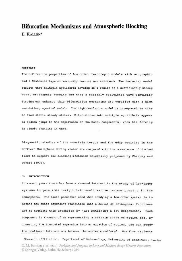
Bifurcation Mechanisms and Atmospheric Blocking E. KALLEN*

Abstract

The bifurcation properties of low order, barotropic models with orographic

and a Newtonian type of vorticity forcing are reviewed. The low order model

results that multiple equilibria develop as a result of a sufficiently strong

wave, orographic forcing and that a suitably positioned wave vorticity

forcing can enhance this bifurcation mechanism are verified with a high

resolution, spectral model. The high resolution model is integrated in time

to find stable steady-states. Bifurcations into multiple equilibria appear

as sudden jumps in the amplitudes of the model components, when the forcing

is slowly changing in time.

Diagnostic studies of the mountain torque and the eddy activity in the

Northern Hemisphere during winter are compared with the occurrence of blocked

flows to support the blocking mechanism originally proposed by Charney and

DeVore (1979).

1. INTRODUCTION

In recent years there has been a renewed interest in the study of low-order

systems to gain some insight into nonlinear mechanisms present in the

atmosphere. The basic procedure used when studying a low-order system is to

expand the space dependent quantities into a series of orthogonal functions

and to truncate this expansion by just retaining a few components. Each

component is thought of as representing a certain scale of motion and, by

inserting the truncated expansion into an equation of motion, one can study

the nonlinear interactions between the scales considered. One thus neglects

*Present affiliation: Department of Meteorology, University of Stockholm, Sweden

D. M. Burridge et al. (eds.), Problems and Prospects in Long and Medium Range Weather Forecasting© Springer-Verlag, Berlin Heidelberg 1984

230

all interactions with spectral components not taken into account. This is of

course a serious limitation of low-order systems, but it is nevertheless

believed that a study of such systems is one way of getting an insight into

the nonlinear mechanisms present in the atmosphere. The models discussed

here only take wave-mean flow interactions into account and this

approximation is discussed by Herring (1963).

When studying a bifurcation problem with a forced, dissipative model the low

order approximation can also be justified as follows. When the forcing is

weak the response is small and the linear dissipative and dispersive terms

dominate over the nonlinear terms which are of a higher order and the model

may be regarded as quasi-linear. For a stronger forcing the response is

increased and the nonlinear terms, which in the models studied here are

quadratic, become increasingly important. In spectral space, a weak forcing

of a certain wavenumber gives a strongly peaked spectrum, while a stronger

forcing distributes energy over a wider range of spectral components. At the

forcing value where the first bifurcation occurs it is thus the spectral

components neighbouring the forced one which are likely to dominate the

nonlinearity. It may then be possible to investigate this first bifurcation

by only taking components into account which are close in spectral space. To

verify results found with a low-order model one should also perform

experiments with a high-resolution, fully nonlinear model. These experiments

must, however, be guided by the qualitative properties of the low-order

system.

To study the effect of orographic forcing on the nonlinear energy transfer

between the larger scales of motion, Charney and DeVore (1979) (hereafter

called CdV) extended Lorenz's (1960) barotropic B-plane model to include

orographic forcing. With a low-order system they showed that for a given

forcing it was possible for the, flow to arrange itself in several equilibrium

231

states, some stable and some unstable. The multiplicity of equilibrium

states is associated with the resonance occurring when the Rossby wave,

generated by the zonal flow over the orography, becomes stationary. Through

the nonlinear interaction between the zonal flow and the wave components of

the flow and due to the orography, the components can arrange themselves in

two stable equilibria, one close to resonance with a large amplitude wave and

a weak zonal flow, the other with a strong zonal flow and a weaker wave

component. The large amplitude wave flow may be associated with a blocked

flow in the atmosphere.

This result was first derived for a 6-plane, channel model with reflecting

side walls, but later studies by Davey (1980,1981) and Kallen (.1981) have

shown that the same type of mechanism can be found with an annular or a

spherical geometry. Trevisan and Buzzi (1980) also showed the same

phenomenon using a different expansion method on a B-plane geometry.

The basic equation used for the models of all these studies is the

quasi-geostrophic, barotropic vorticity equation with linear dissipation, a

Newtonian type of vorticity forcing and orographic forcing. In a

non-dimensional form this equation is

J(I;+ f + h, 1jJ) + e:(I;E - 1;) (1)

where I; is the non-dimensional vorticity, f is the planetary vorticity, I;E

the vorticity forcing, 1jJ the stream function and h is a parameter related to

the orographic effects. The non-dimensional time is given by t and e: is the

dissipation rate. The orographic forcing may be introduced as a forced

vertical velocity of the lower boundary in an equivalent barotropic model, in

which case h is related to a dimensional mountain height m via

h m

C • H (2)

232

where H is the scale height of the equivalent barotropic atmosphere and C is

a constant which depends on the equivalent barotropic assumption. For normal

atmospheric conditions the constant C is approximately equal to one. For

details of the derivation of Eg.(1) see Kallen (1981). To describe the phase

speeds of the long waves properly, a correction term in the time derivative

dependent on the Rossby radius of deformation should be included in Eq.( 1),

(see Wiin-Nielsen, 1959). Since the model is not intended to simulate this

aspect of the long waves with any accuracy the correction term will be

omitted and the equation will be simpler to handle. The correction will only

affect the phase speeds of moving long waves and not the stationary states

which this study mostly deals with.

The nonlinearity of the model is contained in the term involving the Jacobian

(J( ~+ f+h, W», and one way of investigating the nonlinear properties of

this model is to expand the space dependent variables in a series of

orthogonal functions, Fy (~,where ~ is the space vector. It is convenient

to choose the Fy'S to be eigenfunctions of the Laplacian operator, because

~= V2~ The exact functional form of the F 's of course depends on the y

geometry of the model and the boundary conditions.

The variables to be expanded are the vorticity (also g~ves the

streamfunction), vorticity forcing and the orography. The expansion may be

written

I (3) y

For a ~plane, channel model trigonometric functions can be used and

F m,n i(mx+ny) .

(x,y) = e , x and y be~ng the Cartesian coordinates (CdV).

233

In an

annular geometry, Bessel functions are involved (see Davey, 1981) and on the

sphere the F y' S may be written

imA e (4)

where lJ is the sine of latitude (.p), A is the longitude and P m (lJ) are n

associated Legendre functions. Most of the results discussed in this paper

will refer to a spherical geometry as in Kall~n (1981) and thus the expansion

functions given by Eq.(4) are the appropriate ones.

A low-order model may be formulated by inserting the expansion El:J.. ( 3) in the

model El:J.. ( 1) and truncating the expansion at a very low order just leav ing a

few components to describe the fluid motion. Each component may be thought

of as describing a certain scale of motion and only the nonlinear

interactions between the scales involved in the low order system are taken

into account.

To study the effects of the orography on the interaction between the waves

and the mean zonal flow, at least one purely zonal component and two wave

components have to be included. The mathematical structure of such a minimal

system is independent of the geometry and multiple equilibrium states may be

found even in such a simple model, as first pointed out by CdV. When

additional components are included the geometry will affect the structure of

the equations, but the basic mechanism for the formation of multiple

equilibrium states still remains. In the following section a minimal system

will be analyzed, following the basic idea of CdV. Section 3 will deal with

a combination of orographic and direct wave vorticity forcing as discussed by

Kallen (1981). The direct wave vorticity forcing is thought to represent the

time mean effect of the small scale baroclinic eddies on the long waves in

the atmosphere. The effect of baroclinicity is thus taken into account only

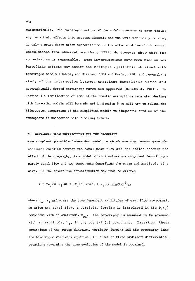
234

parametrically. The barotropic nature of the models prevents us from taking

any baroclinic effects into account directly and the wave vorticity forcing

is only a crude first order approximation to the effects of baroclinic waves.

Calculations from observations (Lau, 1979) do however show that the

approximation is reasonable. Some investigations have been made on how

baroclinic effects may modify the multiple equilibria obtained with

barotropic models (Charney and Strauss, 1980 and Roads, 1980) and recently a

study of the interaction between transient baroclinic waves and

orographically forced stationary waves has appeared (Reinhold, 1981). In

Section 4 a verification of some of the drastic assumptions made when dealing

with low-order models will be made and in SectionS we will try to relate the

bifurcation properties of the simplified models to diagnostic studies of the

atmosphere in connection with blocking events.

2. WAVE-MEAN FLOW IRrERACrIONS VIA THE OROGRAPHY

The simplest possible low-order model in which one may investigate the

nonlinear coupling between the zonal mean flow and the eddies through the

effect of the orography, is a model which involves one component describing a

purely zonal flow and two components describing the phase and amplitude of a

wave. On the sphere the streamfunction may thus be written

where uo ' x 1 and Y1are the time dependent amplitudes of each flow component.

To drive the zonal flow, a vorticity forcing is introduced in the P1(~)

component with an amplitude, UoE ' The orography is assumed to be present

with an amplitude, h 1 , in Inserting these

expansions of the stream function, vorticity forcing and the orography into

the barotropic vorticity equation (1), a set of three ordinary differential

equations governing the time evolution of the model is obtained,

u = hl °1 Yl + c(u -0 DE

Xl (B-a. u o ) y 1 - EX 1

Yl -hi °2 u - (B- a. u ) x - EY 1 o 0 1

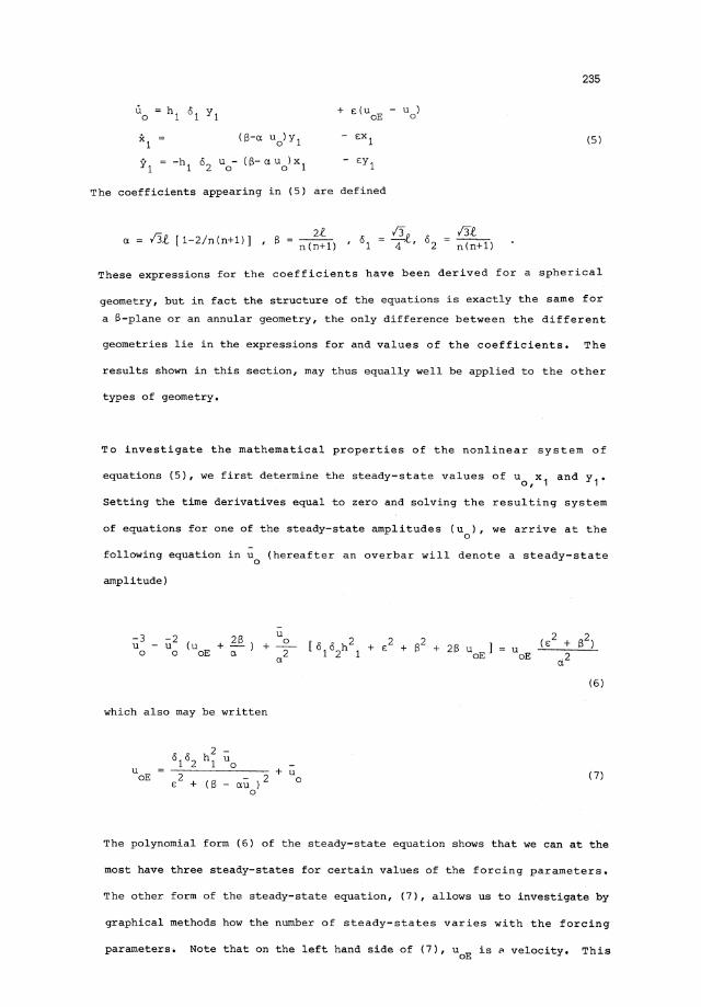
The coefficients appearing in (5) are defined

a. = 13£ [1-2/n(n+l)] , B 2£

n(n+l)

235

u ) 0

(5)

° = /3£ 2 n(n+l)

These expressions for the coefficients have been derived for a spherical

geometry, but in fact the structure of the equations is exactly the same for

a B-plane or an annular geometry, the only difference between the different

geometries lie in the expressions for and values of the coefficients. The

results shown in this section, may thus equally well be applied to the other

types of geometry.

To investigate the mathematical properties of the nonlinear system of

equations (5), we first determine the steady-state values of u o ,x1 and Y1.

Setting the time derivatives equal to zero and solving the resulting system

of equations for one of the steady-state amplitudes (uo )' we arrive at the

following equation in Uo (hereafter an overbar will denote a steady-state

amplitude)

;:i3 _ li2 (u + ~ ) o 0 oE a.

which also may be written

u oE

u DE

(6)

(7)

The polynomial form (6) of the steady-state equation shows that we can at the

most have three steady-states for certain values of the forcing parameters.

The other form of the steady-state equation, (7), allows us to investigate by

graphical methods how the number of steady-states varies with the forcing

parameters. Note that on the left hand side of (7), u oE is C' velocity. This

236

velocity is the purely linear response of the u -component when there is no o

orography.

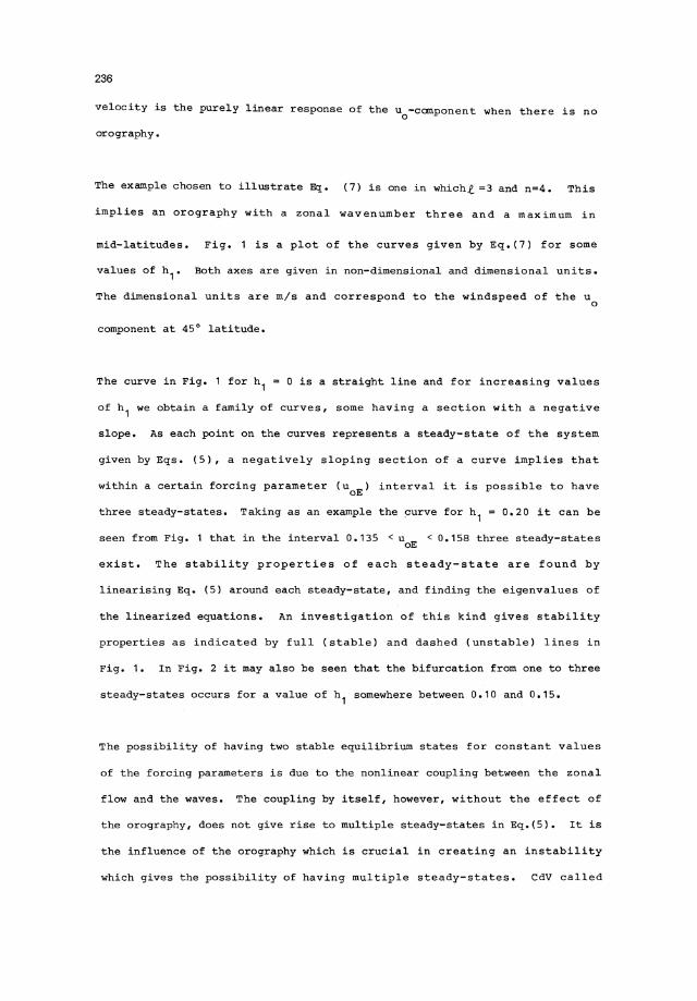
The example chosen to illustrate Eq. (7) is one in which,t =3 and n=4. This

implies an orography with a zonal wavenumber three and a maximum in

mid-latitudes. Fig. 1 is a plot of the curves given by Eq.(7) for some

values of h 1• Both axes are given in non-dimensional and dimensional units.

The dimensional units are m/s and correspond to the windspeed of the Uo

component at 45° latitude.

The curve in Fig. 1 for h1 = 0 is a straight line and for increasing values

of h1 we obtain a family of curves, some having a section with a negative

Slope. As each point on the curves represents a steady-state of the system

given by Eqs. (5), a negatively sloping section of a curve implies that

within a certain forcing parameter (UOE ) interval it is possible to have

three steady-states. Taking as an example the curve for h1 = 0.20 it can be

seen from Fig. 1 that in the interval 0.135 < uOE < 0.158 three steady-states

exist. The stability properties of each steady-state are found by

linearising Eq. (5) around each steady-state, and finding the eigenvalues of

the linearized equations. An investigation of this kind gives stability

properties as indicated by full (stable) and dashed (unstable) lines in

Fig. 1. In Fig. 2 it may also be seen that the bifurcation from one to three

steady-states occurs for a value of h1 somewhere between 0.10 and 0.15.

The possibility of having two stable equilibrium states for constant values

of the forcing parameters is due to the nonlinear coupling between the zonal

flow and the waves. The coupling by itself, however, without the effect of

the orography, does not give rise to mUltiple steady-states in Eq.(5). It is

the influence of the orography which is crucial in creating an instability

which gives the possibility of having mUltiple steady-states. CdV called

237

1'4

= 1'2

1'0

I 50 mls 0

0'8 ~

uJ 0 :::l 0'6

0'4 -stable

- - - unstable

0'2

50 mls 0'0 L-_'--_"--_.L.-_..L....I_..L-_..L-_..L--

0'0 0'2 0'4 0'6 0'8 1'0 1'4

Fig. 1. Steady-state curves for the low order model of section 2 with different values of the orographic parameter. The horizontal axis gives the ampli­tude of the uo-component, both in non-dimensional and dimensional units. On the vertical axis the forcing is also given in both units. The dimensional units are the flow velocity at 450 latitude. Each curve corresponds to a certain value of the orographic parameter, h1' and a numerical evaluation of the eigenvalues shows stability properties as indicated by full (stable) and dashed (unstable) lines. For further explanations, see text. Parameter values: £ = 0.06, ~ = 3, n1= 4

238

this a form drag instability, where the form drag refers to the effect of the

orography in this simple model.

One of the stable steady-states is close to a resonant flow configuration,

and in this steady-state the wave component has a high amplitude. The phase

of the wave is such that there is a high drag across the orographic ridges

and thus energy is transferred from the zonal forcing, via the effect of the

orography, to the wave components of the flow. In Fig. 1 this type of a

steady-state falls on the left hand part of the diagram where the response in

the zonal component (uo ) is much less than the forcing.

The steady-states on the right hand side of the unstable region have a more

intense zonal flow and a less marked wave component. In these steady-states

the orographic drag is much lower, both due to the lower amplitude of the

wave component and a different phase of the wave.

The steady-state with a high wave amplitude may be associated with a blocked

flow in the atmosphere. The wave ridge occurs downstream of the orographic

ridge, and the persistence of blocking ridges in the atmosphere may be due to

the stable wave-mean flow interaction described by this simple model. The

model also predicts that tnere may be another stable flow configuration

without a high amplitude wave, but a much more pronounced zonal flow. Which

one of these steady-states the flow settles into is crucially dependent on

the initial state of the flow. CdV offered this feature as a possible

explanation for the observed variability in the frequency of the occurrence

of blocked flows.

239

3. A COMBINATION OF WAVE VORTICrry AND OROGRAPHIC FORCING

In the model described in the previous section, the waves of the flow are

only due to the interaction between the zonal flow and the orography. In the

atmosphere there are numerous other processes which generate waves and in

midlatitudes the most important one is the baroclinic instability process.

Baroclinic waves have a characteristic wavelength which is shorter than the

scales involved in the low order models of this study, but seen as an effect

on the time mean flow the energy generated by baroclinically unstable waves

on the shorter scales is transported in the spectrum through nonlinear

processes and thus also exports kinetic energy to the longer waves

(Saltzmann, 1970 and Steinberg et al, 1971). In a barotropic model it is

impossible to describe these baroclinic effects explicitly, but as a first

approximation one may be able to take the long wave effect into account by

introducing a wave vorticity forcing in the same components as the orography.

The wave vorticity forcing should thus be seen as the time mean effect of

cyclone waves rather than a direct diabatic heating.

A wave vorticity forcing can easily be introduced into the low order model of

the previous section by adding €H 1E and EylE to the right hand sides of the

equations for *1 and y 1 of Eq. (5). The steady-states may be analyzed in the

same way by writing the steady-state equation in terms of the zonal forcing

(UOE ) as a function of the zonal response

amplitude ("lE2 + Y1E2 ) and the phase

(uo ) with the orography (h 1), the

(tan -lYlE) of the wave vorticity x1E

forcing as parameters. In Kallen (1981) this was done, but with a sightly

more complicated model. Two extra wavecomponents and one extra zonal

component was included to take into account some of the interactions with

unforced parts of the spectrum. It is still possible to solve for the

steady-states analytically in such a model according to the procedure given

in K!llen (1981). We will not go into any detail here regarding the solution

method, but only display some of the results.

240

The streamfunction expression used in the examples is

I/J (fi, A, t)

+ 3 (xl (t) cos 3A + Yl (t) sin 3A) P4 (fi) +

+ sin

and the vorticity forcing is given by

+ (X 1E cos 3A + Y lE sin 3

3A) P 4 (fi)

The orography is the same as in the previous section,

The low order system is thus made up of six ordinary differential equations,

which govern the time evolution of the model. Because of the choice of

components, no direct wave-wave to wave interactions are allowed but energy

transfer from one wave-component to the other may take place via the zonal

flow. The zonal component with the amplitude z describes a sheared zonal

flow and it is via this zonal component that energy may be transferred

through flow-flow interactions from the forced to the unforced wave

components.

241

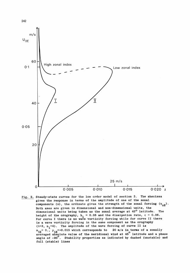
A plot of the steady-states of the system is given in Fig. 2. On the

horizontal axis the steady-state response is given in terms of the amplitude

of the sheared zonal component, z. The vertical axis gives the zonal

momentum forcing, UOE '

The orographic forcing is fixed at a value of 0.05 while the wave vorticity

forcing has a varying amplitude, but the phase in relation to the orography

is fixed. Multiple steady-states of the system are identified in the figure

by the condition that a horizontal line should have multiple intersections

with one of the steady-state curves. The forcing parameters are in a range

where multiple steady states are just possible, i.e. close to the first

bifurcation point. For smaller values of the forcing parameters the

nonlinear system behaves quasi-linearly, with just one steady state for a

certain value of the forcing parameters. By linearizing the system around a

steady-state and computing the eigenvalues of the matrix governing the

linearized motion around each of the steady-states, stability properties are

found as indicated in Fig. 2. It may be noted that no Hopf-bifurcations (see

Marsden and McCracken, 1979) indicating the existence of limit-cycles around

the steady-states have been found in this low order model for reasonable

values of the forcing parameters.

For the curve marked I in Fig. 2 the wave vorticity forcing is set to zero

and the only forcing of the model is in the orography and the zonal momentum.

For the orography height chosen in Fig. 2 there is only one, stable

steady-state for all values of the zonal momentum forcing. For higher values

of the orographic parameter mUltiple steady-states are possible within

certain ranges of values of the zonal momentum forcing. For further details

of this, see Kallen (1981). Another way of obtaining a region of multiple

equilibria is to include vorticity forcing in one of the wave components and

this is shown with steady state curve II in Fig.2. The phase of the wave

vorticity forcing is _90°, i.e. positive (cyclonic) vorticity forcing on the

242

m/s UOE

60

0·1 Low zonal index

40

0·05

25 m/s OL-----------~-------------L------~----~------------~~

0·005 0·010 0·015 0·020 z

Fig. 2. Steady-state curves for the low order model of section 3. The abscissa gives the response in terms of the amplitude of one of the zonal components (z), the ordinate gives the strength of the zonal forcing (uoE). Both axes are given in dimensional and non-dimensional units, the dimensional units being taken as the zonal average at 450 latitude. The height of the orography, hI = 0.05 and the dissipation rate, £ = 0.06. For curve I there is no wave vorticity forcing while for curve II there is a wave vorticity forcing in the same component as the orography (~=3, n l =4). The amplitude of the wave forcing of curve II is x lE= 0., YlE=-o.Ol5 which corresponds to 20 m/s in terms of a zonally averaged absolute value of the meridional wind at 450 latitude and a phase angle of _900 • Stability properties as indicated by dashed (unstable) and full (stable) lines

243

leeward side of the highs in the orography. In Kallen 1981 it was shown that

this phase angle is the most favourable one for bifurcations to occur. The

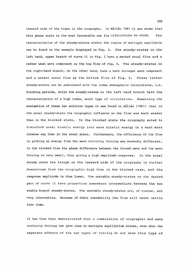
characteristics of the steady-states within the region of mUltiple equilibria

can be found in the example displayed in Fig. 3. The steady-states on the

left hand, upper branch of curve II in Fig. 2 have a marked zonal flow and a

rather weak wave component as the top flow of Fig. 3. The steady-states on

the right-hand branch, on the other hand, have a much stronger wave component

and a weaker zonal flow as the bottom flow of Fig. 3. These latter

steady-states can be associated with low index atmospheric circulations, i.e.

blocking periods, while the steady-states on the left hand branch have the

characteristics of a high index, zonal type of circulation. Examining the

energetics of these two solution types it was found in Kall;n (1981) that in

the zonal steady-state the orographic influence on the flow was much weaker

than in the blocked state. In the blocked state the orography acted to

transform zonal kinetic energy into wave kinetic energy in a much more

intense way than in the zonal state. Furthermore, the efficiency of the flow

in picking up energy from the wave vorticity forcing was markedly different.

In the blocked flow the phase difference between the forced wave and the wave

forcing is very small, thus giving a high amplitude response. In the zonal

steady state the trough on the leeward side of the orography is further

downstream from the orographic high than in the blocked case, and the

response amplitude is thus lower. The unstable steady-states on the dashed

part of curve II have properties somewhere intermediate between the two

stable branch steady-states. The unstable steady-states are, of course, not

very interesting. Because of their instability the flow will never settle

into them.

It has thus been demonstrated that a combination of orographic and wave

vorticity forcing can give rise to multiple equilibrium states, even when the

separate effects of the two types of forcing do not show this type of

244

UNSTABLE

Fig. 3. Examples of stream function fields for three steady-states within the region of possible multiple equilibria of Fig. 2 (curve II). Full lines are isolines of the streamfunction while the dashed lines are isolines for the orography. Over the hatched area the orography is above its mean value ("land areas") while otherwise it is below its mean value ("ocean area"). Dash~dotted curves with arrows showing direction of circulation indicate regions with maximum cyclonic and anti-cyclonic wave vorticity forcing

245

behaviour. With wave vorticity forcing alone this model does not give rise

to more than one equilibrium state. The orography can be seen to act as a

triggering mechanism, directing the basically vorticity forced flow into one

or the other of the stable equilibria.

4. HIGH RBSOLUrION EXPERIllEHrS

A serious shortcoming of a severely truncated low order system is of course

the lack of interaction between waves of all scales. Only a few scales of

motion are taken into account and the interactions with other scales are

either neglected completely or included via a bulk momentum forcing. To

investigate whether the bifurcation mechanism found in a low order model is

sensitive to the number of waves present in the model, the results should in

some way be verified with a high resolution model. CdV showed that the

mUltiple equilibria in their 8-plane channel model could also be found in a

model with an increased resolution, while (Davey 1981) pointed out that it is

possible to find the multiple equilibria in a high resolution model but they

do not obtain as easily as in a low order model.

To verify the results of Kallen (1981) for a spherical geometry, experiments

have been performed with a high resolution (horizontally) quasi-geostrophic,

spectral, barotropic model. These experiments will be described here

following Kallen (1982).

The high resolution model was originally developed at the University of

Reading, UK and it is a barotropic and quasi-geostrophically balanced version

of the model described in Hoskins and Simmons (1975). The governing equation

of the model is the same as in Section 2, i.e. Eq. (1). Forcing is

introduced in exactly the same components as in the low-order model of

Section 3 and the model is integrated in time to find the steady-state(s).

For reasons of economy, most of the experiments were done with a T21

truncation (k ..; 21 and n .;;; 21 in the Legendre (P k (iJ.» representation). n

246

However, some integrations done with a T42 truncation showed no significant

differences to the T21 experiments.

To find multiple stable steady-states the time integrations are set up in the

following manner. Initially the forcing is held constant for a time period

of twenty days. The model, starting from a state of rest, is allowed this

time to find a steady-state. After the model has settled into a steady-state

the zonal momentum forcing is slowly increased or decreased in time. The

time scale (/)f this slow increase or decrease is chosen to be significantly

slower than the dissipation time scale of the model (the forcing is doubled

or halved in 100 days while the dissipation time scale is around 2.5 days).

With this rather large dissipation rate the model stays reasonably close to a

stable steady-state all of the time. If, however, a bifurcation of the type

pictured in Fig. 2 occurs, the model has to make a sudden jump from one

stable branch of the steady-state curve to the other when a critical value in

the zonal forcing is passed. In a time plot of some of the spectral

coefficients this will show up as a sudden" change of the amplitude and

perhaps some damped oscillations when the model settles into a steady-state

on the other branch.

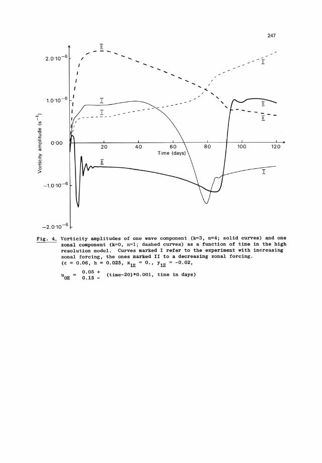
Results of experiments of this type are displayed in Fig. 4. The forcing

parameters have values which are close to the ones used in the low order

example of Fig. 2. The phase difference between the wave vorticity forcing

and the orography is exactly the same, -90°. It was, however, found that in

order to obtain multiple equilibrium states with a high resolution model the

vorticity forcing has to be higher. This is presumably due to the fact that

the existence of more components forces the energy introduced at certain wave

components to spread out to all parts of the spectrum. The long waves,

therefore need more energy input to reach the critical amplitudes necessary

for bifurcations to occur. The orography, on the other hand, had to be

247

IT

2.0.10-6 ."

I ..... .....

I ..... ... I

..... ... , ....

1.0.10-6 ,

I , .... , , I

'I -------.:E.

,

" Q)

"C

.~ 0. 0·00 E 20 '" ~ ·u

.IT .~

>

-1.0.10-6

Fig. 4. Vorticity amplitudes of one wave component (k=3, n=4; solid curves) and one zonal component (k=O, n=1; dashed curves) as a function of time in the high resolution model. Curves marked I refer to the experiment with increasing zonal forcing, the ones marked II to a decreasing zonal forcing. (E = 0.06, h = 0.025, x1E = 0., Y1E = -0.02,

0.05 + uOE = 0.15 _ (time-20)*0.001, time in days)

248

lowered to avoid the formation of mUltiple equilibria when only zonal

momentum forcing is present. The high resolution model thus appears to be

more sensitive to the height of the orography than the low order model.

In Fig. 4 the amplitudes of the forced zonal and wave components are shown as

functions of time for two different experiments. In one experiment (curves

marked I) the zonal forcing starts at a fairly low value, well below the

bifurcation "knee" of the curve in Fig.2. After day 20 the zonal forcing is

increased slowly and from the amplitudes of the forced zonal component and

the forced wave component it can be seen that a sudden jump occurs around day

80. The curves marked II show a similar experiment, but this time the zonal

forcing is decreasing as a function of time. In these curves the jump occurs

around day 90 and it should be noted that the jump does not occur at the same

v·alue of the zonal forcing as for the jump with an increasing zonal forcing.

This strongly suggests that there is a certain interval in the values of the

ztmal forcing where multiple stable steady-states are possible. To find

these steady-states the same type of integrations have been performed, but

instead of increasing/decreasing the zonal forcing until the end of the

inte';l"ration the zonal forcing was held constant at a certain level after an

increase/decrease from an initially low/high value. The final level of the

forcing was chosen to be in the range of possible multiple equilibria. In

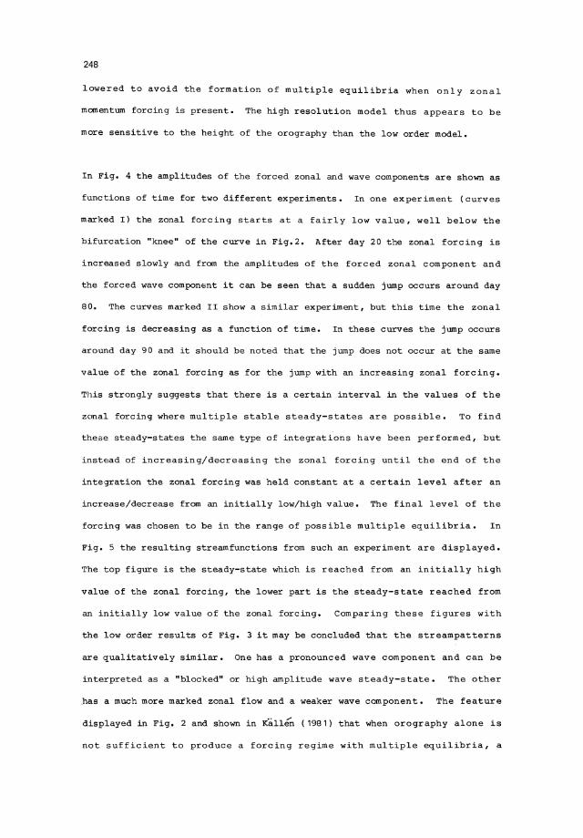
Fig. 5 the resulting streamfunctions from such an experiment are displayed.

The top figure is the steady-state which is reached from an initially high

value of the zonal forcing, the lower part is the steady-state reached from

an initially low value of the zonal forcing. Comparing these figures with

the low order results of Fig. 3 it may be concluded that the streampatterns

are qualitatively similar. One has a pronounced wave component and can be

interpreted as a "blocked" or high amplitude wave steady-state. The other

.has a much more marked zonal flow and a weaker wave component. The feature

displayed in Fig. 2 and shown in Kalle'n (1981) that when orography alone is

not sufficient to produce a forcing regime with multiple equilibria, a

249

Fig. 5. Two stable streamfunction patterns having the same values of all the forcing parameters (e = 0.06, h = 0.025, x lE = 0.0, YIE = -0.02, uOE = 0 . 095). Full lines are isolines for the streamfunction with the same isoline interval in the two plots. Dashed lines are isolines for the orography, areas with the orography above its mean value (land areas) are hatched. The dashed-dotted curves indicate the positions and directions of maximum and minimum wave vorticity forcing

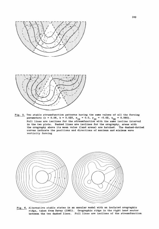
Fig . 6. Alternative stable states in an annular model with an isolated orographic ridge, taken from Davey (1981). Orographic ridge in the right hand sector between the two dashed lines. Full lines are isolines of the streamfunction

250

combination of orographic and wave vorticity forcing does give this

possibility, is reproduced by the high resolution model. The addition of

wave vorticity forcing is thus not just a linear addition of wave energy to

the flow, instead it actively takes part in the nonlinear formation of

multiple equilibria.

The numerical experiments with the high resolution spectral model thus

strongly support the results derived from the low order model of Kallen

(1981). There are, however some aspects of the low order model behaviour

which are not verified by the high resolution experiments. One such

behaviour is the bifurcation obtained in a low order model in the absence of

orography. With a five component low order model it is possible to find

multiple equilibria with only vorticity forcing (Wiin-Nielsen, 1979) on the

longer waves. Experiments with the high resolution model have not shown this

feature, even for very large values of the forcing parameters. The model

behaves perfectly linear when only momentum forcing is applied, the response

to the forcing being purely in the forced components. For shorter waves this

is no longer true. Hoskins (1973) has demonstrated that for zonal

wavenumbers larger than five a nonlinear instability develops which is mainly

due to wave-wave interactions. For the longer waves the beta-effect acts as

a stabilizing factor which prevents this type of nonlinear instability. With

orography present it thus seems that a new type of instability develops as

first pointed out by CdV. An intuitive reasoning which points to a possible

reason for this property of the orography can be given as follows. The

governing equation of the model at a steady-state may be written

'illjJ J(~,ljJ) + J(h,ljJ) - 2aI + E(~E - ~) o (8)

If h=O (no orographic forcing) and ~Ef'O it is possible to have a steady-state

where the response is in the same component as the forcing and the nonlinear

251

term J( ~,~) is zero. As mentioned above, numerical experiments with

reasonable values of the vorticity forcing on the longer waves have shown

that such a steady-state is stable. Equation (8) is in this case linear.

This also holds if the wave vorticity forcing is applied at several low wave

numbers simultaneously. If an orographic forcing is introduced (hi 0) the

term J(h,~) forces energy introduced via the vorticity forcing ~E at a

certain wavenumber to spread over the whole spectrum. It is this energy

spread combined with a suitable vorticity forcing that appears to give rise

to a nonlinear instability and the bifurcation leading to mUltiple

steady-states. The experiments with the high resolution model have also

confirmed that a suitably positioned vorticity forcing in a wave component

enhances this bifurcation mechanism.

Another aspect of using one Fourier component to represent the orography

which can be tested with a high resolution model, is to see whether multiple

equilibria can be obtained with an isolated orographic ridge. Davey (1981)

did an experiment of this type with an annular geometry and within a certain,

rather narrow, range of the forcing parameter space, he obtained multiple

steady-states. An example of two stable states can be found in Fig. 6.

These states have the same characteristics as the blocked and zonal states

described previously. It can also be seen from Fig. 6 that in the high

amplitude wave state the waves generated on the leeward side of the

orographic ridge are almost totally dissipated when the flow reaches the

upwind side of the orographic ridge. The high amplitude wave state is thus

not associated with a global resonance, the phenomenon is rather local in

character. The resonance occurring is instead of the type where the Rossby

wave generated by the orography has a phase speed which is such that it is

stationary in the zonal flow which results.

252

5. OBSERVATIONAL BrUDXES SUPPORUNG A BIFURCATION MECHARISM FOR BIDCKXRG

The main conclusion that can be drawn from the bifurcation mechanism found in

barotropic models is that the orography is necessary as a triggering

mechanism in establishing the mUltiple steady-states. The implied

application of the theory to atmospheric blocking can thus be tested by

studying the effect of the orography on the atmospheric flow in connection

with blocked flow situations. One parameter which reflects the influence of

the orography on the barotropic component of atmospheric flow is the mountain

torque. To furthermore couple observational evidence with the combination of

orographic and wave vorticity forcing, an evaluation of the long wave forcing

is needed. This forcing should be seen as the cumulative effect of the

transient eddies on the mean flow rather than a direct thermal forcing.

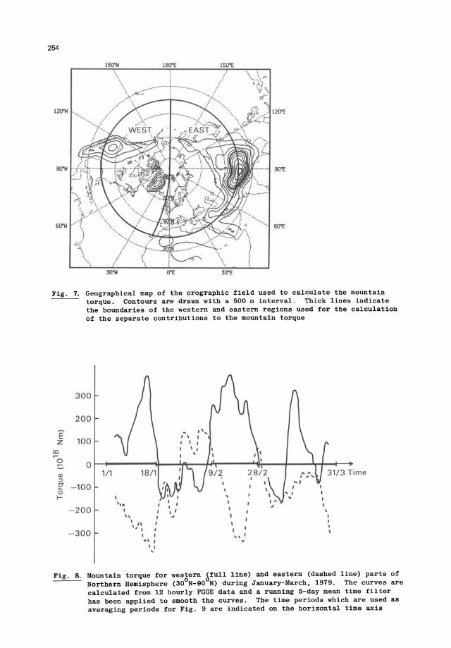
To study the orographic factors influencing blocking action in the Atlantic

and Pacific regions separately it is necessary to separate the torque

contributions from the American and the Eur-Asian continents. It is

primarily downstream from a mountain range that the orography may influence

the flow pattern. The mountain torque parameter essentially reflects the

surface pressure distribution around a mountain range and therefore it would

be possible to separate the contributions from each continent by computing

the torque for the eastern and western parts of the Northern Hemisphere

separately. The separation line between eastern and western parts would then

have to lie entirely within the oceanic regions. Computations of the

mountain torque around complete latitute circles has previously been done by

Oort and Bowman (1974). They presented monthly averaged results for a five

year period including the anomalous winter of 1963. In January 1963 there

was a well developed blocking ridge over the Atlantic region (see O'Connor,

1963) and for this month there was an exceptionally high mountain drag in

midlatitudes. Recent calculations by Metz (private communication) have also

shown a correlation between high values of the mountain drag (again around

253

complete latitude circles) and high amplitudes of the geopotential over the

eastern Atlantic area.

Separating the torque contributions from the North American and the Eur-Asian

continents, Kallen (1982) has shown that during one winter period

(January-March, 1979) there is a correspondence between a mountain drag and

the occurrence of a blocking ridge downstream of the mountain barrier.

The mountain drag, TM, is defined as

- f A

P s

dh dA a cos~ dS (9)

where ps is the surface pressure, h the surface elevation above sea level, a

the radius of the earth and ~, Athe latitudinal and longitudinal coordinates,

respectively. The integration is carried out over two areas, one containing

the North American continent and another containing the Eur-Asian continent.

Both areas extend from the North Pole down to 30 o N. The separation lines

between the two areas lie entirely within oceanic regions and the torque

contributions from both continents can thus be evaluated separately (Fig. 7).

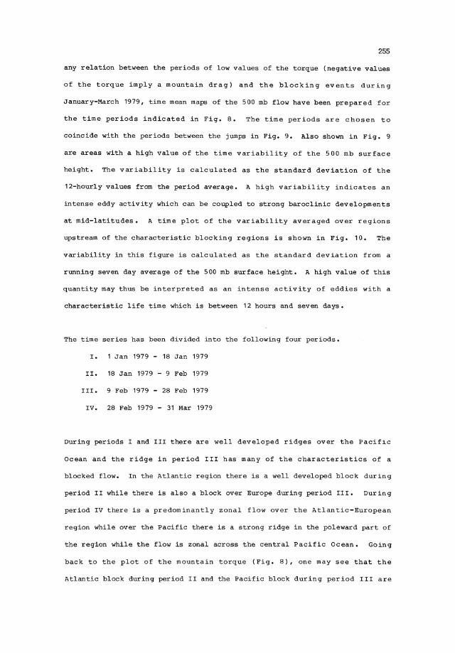
A time plot of the torque for the two areas is shown in Fig. 8. The time

evolution of the mountain torque has been smoothed with a five day running

time mean to remove the influence of short lived, travelling baroclinic

eddies. These tend to give large variations in the torque on a time scale of

one day.

The most prominent feature of the curves in Fig. 8 is the large variation of

the torque on a time scale of about two weeks. Both curves tend to show

sudden jumps between what appears to be fairly constant values, the jumps

appearing over a time interval which is shorter than the time scale over

which the torque is approximately constant. To investigate whether there is

254

Fig. 7. Geographical map of the orographic field used to calculate the mountain torque. Contours are drawn with a 500 m interval. Thick lines indicate the boundaries of the western and eastern regions used for the calculation of the separate contributions to the mountain torque

E z

CO .... 0 ::: Q> :> 0" (;; I-

300

200

100

0 1/1

- 100

,,- I - 200 • I

I

" I , ,

, 1\

- 300 ~ I

I ~,

~, I , I ~

Mountain torque for western (full line) and eastern (dashed line) parts of Northern Hemisphere (30oN_90oN) during January-March, 1979. The curves are calculated from 12 hourly FGGE data and a running 5-day mean time filter has been applied to smooth the curves. The time periods which are used as averaging periods for Fig . 9 are indicated on the horizontal time axis

any relation between the periods of low values of the torque (negative values

of the torque imply a mountain drag) and the blocking events during

January-March 1979, time mean maps of the 500 mb flow have been prepared for

the time periods indicated in Fig. 8. The time periods are chosen to

coincide with the periods between the jumps in Fig. 9. Also shown in Fig. 9

are areas with a high value of the time variability of the 500 mb surface

height. The variability is calculated as the standard deviation of the

12-hourly values from the period average. A high variability indicates an

intense eddy activity which can be coupled to strong baroclinic developments

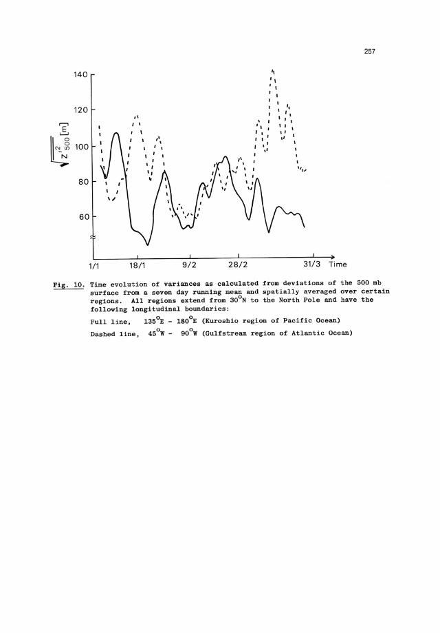
at mid-latitudes. A time plot of the variability averaged over regions

upstream of the characteristic blocking regions is shown in Fig. 10. The

variability in this figure is calculated as the standard deviation from a

running seven day average of the 500 mb surface height. A high value of this

quantity may thus be interpreted as an intense activity of eddies with a

characteristic life time which is between 12 hours and seven days.

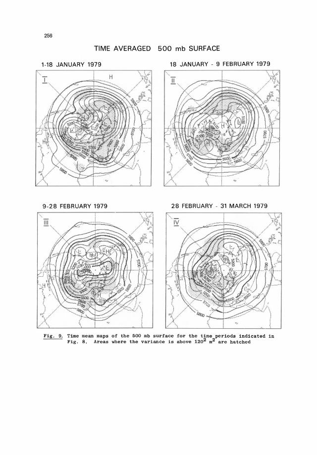
The time series has been divided into the following four periods.

I. 1 Jan 1979 - 18 Jan 1979

II. 18 Jan 1979 - 9 Feb 1979

III. 9 Feb 1979 - 28 Feb 1979

IV. 28 Feb 1979 - 31 Mar 1979

During periods I and III there are well developed ridges over the Pacific

Ocean and the ridge in period III has many of the characteristics of a

blocked flow. In the Atlantic region there is a well developed block during

period II while there is also a block over Europe during period III. During

period IV there is a predominantly zonal flow over the Atlantic-European

region while over the Pacific there is a strong ridge in the poleward part of

the region while the flow is zonal across the central Pacific Ocean. Going

back to the plot of the mountain torque (Fig. 8), one may see that the

Atlantic block during period II and the Pacific block during period III are

256

TIME AVERAGED 500 mb SURFACE

1-18 JANUARY 1979 18 JANUARY - 9 FEBRUARY 1979

9-28 FEBRUARY 1979 28 FEBRUARY - 31 MARCH 1979

Fig. 9. Time mean maps of the 500 mb surface for the time periods indicated in Fig. 8. Areas where the variance is above 1202 m2 are hatched

140

120

,......, S

~ 100

80

60

1 1/1

\~

,I , . " ,

• I ,

18/1 9/2 28/2

, '. , , I I

, I

"

" , , , ,

" " • I

• I

I'

"

257

31/3 Time

Fig. 10. Time evolution of variances as calculated from deviations of the 500 mb surface from a seven day running mean and spatially averaged over certain regions. All regions extend from 300 N to the North Pole and have the following longitudinal boundaries:

Full line, 1350 E 1800 E (Kuroshio region of Pacific Ocean)

Dashed line, 450 W - 900 W (Gulf stream region of Atlantic Ocean)

258

coupled with low, negative values of the torque, i.e. a mountain drag. The

Pacific ridge during period I is also associated with a high mountain drag

over the Eur-Asian continent while the zonal flows over the Atlantic region

during periods I and III and over the Pacific during period II are coupled

with high, positive values of the torque. During the last period (IV) the

torque from the North American continent shows considerable fluctuations and

the flow over the Atlantic and European regions is predominantly zonal. The

torque from the Eur-Asian continent is distinctly negative and there is a

ridge extending northwards towards the polar regions over the Pacific Ocean.

The occurrence of a high mountain drag thus has some correspondance with the

appearance of a blocking high downstream of a continent.

The influence of the transient motion on the time mean flow is the mechanism

which in the barotropic model is represented by a direct vorticity forcing.

Evaluating this vorticity forcing from atmospheric data is difficult as

discussed by Savijarvi (1978). Some attempts have been made at calculating

the vorticity forcing for the time periods indicated in Fig. 8, but the

results have generally been noisy and it has been difficult to see any clear

pattern. Instead, the eddy activity has been evaluated in terms of the

standard deviation of the 500 mb surface during the different time periods.

From Fig. 9 it may be seen that the eddy activity upstream of a blocking

region has some connection with the time periods defined earlier. Through

Fig. 10 it may be seen that the Atlantic blocking during period II and to

some extent the Pacific blocking during period III are coupled with a strong

eddy activity in the beginning of those periods. However, as the blocking

period continues there seems to be a decline in the activity of the eddies,

especially during period II and in the Atlantic region. The decay of the

block m~y therefore be coupled with the declining eddy activity, when the

block has disappeared there is a renewed intensification of the eddy

activity. This process is clearly baroclinic and the barotropic model of the

259

previous sections cannot simulate it. It would be of interest to see if a

simple baroclinic model could show these effects in the presence of

orography. The reasoning does not hold with the period III block in the

Pacific region, there the blocking is preceded by a very low eddy activity.

On the geographical maps (Fig. 9) it may however be seen that there is a

small region with a fairly high eddy activity just upstream of the block and

it may be that the procedure of averaging the variance over a large area

smooths this feature out. In any case, the geographical maps clearly show

that the upstream flanks of the blocked regions do have intense eddy activity

on the average and this is to be expected from the well known fact that in

the Gulfstream and Kuroshio regions of the Atlantic and Pacific Oceans

respectively, there is normally an intense baroclinic activity.

The ridge over F;urope during period III, which on the daily 500 mb maps can

be associated with blocking like patterns, is not connected with a high

mountain drag over the American continent. This may be explained by the fact

that the ridge is too far downstream from the orography to be significantly

influenced by it and the blocking ridges may therefore develop due to some

other mechanism. From the plot of the variance of the 500 mb surface

(Fig. 7) it may however be noted that within the European area there is quite

a large variability during this time period. This can be due to blocking

like ridges moving across the area and not remaining stationary which also

gives a smoothed ridge on a time averaged map. It may thus be a situation in

which transient ridges develop, but because of the orientation of the large

scale flow and the effect of the orography, the ridges cannot remain

stationary to form a persistent block.

260

6. DISCUSSION

Investigations of the nonlinear properties of simplified atmospheric models

have shown that a combination of orographic and vorticity forcing in

barotropic, quasi-geostrophic models gives rise to a long wave instability

and the development of multiple, stable equilibrium states. One of these

stable states can be associated with a large amplitude wave response, while

another has a dominating zonal flow and a less pronounced wave component.

The large amplitude wave response (or blocked response) is close to a

resonant flow configuration, where the wave response is almost in phase with

the wave forcing. The zonal steady state is further removed from resonance

and the response in the wave component is much weaker. Instead, due to the

changed phase relationship between the wave and the orography, the zonal flow

is more intense and the mountain drag is lower. These two types of

equilibria can exist for the same values of all the forcing parameters, which

one the flow choses is crucially dependent on the initial state of the flow

in relation to the unstable steady-state.

The forcing parameters required in the barotropic model for the development

of multiple equilibria, can be associated with the conditions present in the

Northern Hemisphere during wintertime. A strong zonal flow and an intense

baroclinic eddy activity off the eastern coasts of the two major continents

can thus be linked with two possible types of response of the long waves in

the atmosphere. Once the atmosphere has settled into one of these response

types it is likely to remain there for an extended period of time due to the

stability of the flow configuration. In one of the response types there is a

well developed ridge downstream of a continent and this ridge can be

associated with a blocked flow. To remain in this near resonant flow

configuration it is also necessary that the eddy activity upstream of the

blocking ridge is maintained to give an input of kinetic energy on the long

waves. Fram the diagnostic studies of Kallen (1982) it appears that this

eddy activity steadily decreases during a blocking event and this may be the

261

cause for the vanishing of the blocking ridge. A decreased eddy activity

would, according to the barotropic mechanism put forward in Section 3, imply

that the blocked steady-state vanishes (for a constant zonal forcing) and the

flow is forced to settle into a zonal flow configuration. In Fig. 2 this may

be visualized as the disappearance of curve II when the flow has settled into

a state on the high index branch of curve II. At a critical value of the

eddy forcing of the long waves the flow would be forced to transfer to a more

zonal type of circulation.

A similar way in which cyclonic eddies and the orography may interact has

been studied by Kalnay-Rivas and Merkine (1981). They investigated the

effect of isolated vortices when periodically released upstream of an

orographic ridge in a barotropic flow. A resonant, blocked type of response

was found downstream of the orography when the time-averaged wave generated

by the cyclonic eddy forcing was in phase with the orographically generated

Rossby wave. This is the same type of reinforcing interaction which has been

described in this paper, although Kalnay-Rivas and Merkine (1981) did not

find any multiple equilibrium due to the nonlinear interactions. Instead

they emphasized the effect of the nonlinarity in producing an n-shaped

blocking pattern.

Recent investigations by Lau (1981) and Volmer et al (1981) on the behaviour

of the GFDL and. E~WF general circulation models in long time integrations

have interesting connections with the bifurcation mechanism discussed here.

The data from the long integrations were analysed through an expansion into

empirical orthogonal functions. Lau (1981) showed that he could find two

characteristic types of wintertime circulations in the Northern Hemisphere,

one with a predominantly zonal flow and another with a more pronounced

meridional flow. Examining the variance during these two characteristic

types of months, Lau (1981) was also able to show that the cyclone tracks

262

over the Pacific and North Atlantic Oceans were very different during these

months. During the months with a high zonal index the regions with a high

variance extended across the oceans, while during the months with a low zonal

index the variance was high only over the eastern parts of the oceans. It

thus seems that the model has two different modes of circulation during

wintertime in the Northern Hemisphere and the characteristic properties of

these modes agree quite well with those of the two stable states found in a

simple, low order, barotropic model.

References

Charney, J.G. and DeVore, J.G. 1979 Multiple flow equilibria in the atmosphere and blocking. ~.Atmos.Sci., 36, 1205-1216.

Charney, J.G. and Strauss, D.M. 1980 Form-drag instability, multiple equilibria and propagating planetary waves in baroclinic, orographically forced, planetary wave systems. ~.~.Sci., 37, 1157-1176.

Davey, M. K. 1980 A quasi-linear theory for rotating flow over topography. Part I: Steady -plane channel. ~.Fluid Mech., 99, 267-292.

Davey, M.K. 1981 A quasi-linear theory for rotating flow over topography. Part II: Beta-plane annulus. ~.Fluid Mech., ~, 297-320.

Herring, J.R. 1963 Investigation of problems in thermal convection. ~.AtmoS.Sci.,~, 325-338.

Hoskins, B.J. 1973 Stability of the Rossby-Haurwitz wave. Quart.~.~.Met.Soc., 99, 723-745.

Hoskins, B.J. and Simmons, A.J. 1975 A multi-layer spectral model and the semi implicit method. Quart .~.~.Met.Soc., ~, 637-655.

Kalnay-Rivas,E. and Merkine, L.O. ~.AtmoS.Sci., ~, 2077-2091.

1981 A simple mechanism for blocking.

Kalle;,E. 1981 The nonlinear effects of orographic and momentum forcing in a low-order ,barotropic model. ~.Atmos .Sci., ~, in press.

Kallen ,E. 1982 Bifurcation properties of quasi-geostrophic, barotropic models and the relation to atmospheric blocking. Tellus, in press.

Lau,N.C. 1981 A diagnostic study of recurrent meteorological anomalies appearing in a 15-year simulation with a GFDL general circulation model. Mon.Wea.Rev., ~, 2287-2311.

Lorenz, E.N. 1960 Maximum simplification of the dynamic equations. Tell us, ..!3,., 243-254.

Marsden, J.E. and McCracken, M. 1976 The Hopf bifurcation and its applications. Springer Verlag, New York, pp.408.

263

O'Connor, J.F. 1963 The weather and circulation of January 1963. Mon.Wea.Rev., ~, 209-218.

Oort, A. H. and Bo=an, H.D. 1974 A study of the mountain torque and its interannual variations in the Northern Hemisphere. ~.Atmos.Sci.,~, 1974-1982.

Reinhold, Brian B., Pierrehumbert, Raymond T., 1982 "Dynamics of weather regimes: quasi-stationary waves and blocking", Mon.Wea.Rev., 11.£, 1105-1145.

Roads,J.O. 1980 Stable near-resonant states forced by orography in a simple baroclinic model. ~.Atmos.Sci., E, 2381-2395.

Saltzmann, B. 1970 Large-scale atmospheric energetics in wave-number domain. Rev. of Geophysics and Space Physics, ~, 289- 302.

Savijarvi, H. 1978 The interaction of the monthly mean flow and large scale transient eddies in two different circulation types, Part II.

Geophysica, li, 207-229.

Steinberg, H.L., Wiin-Nielsen, A. and C.-H. Young 1971 On nonlinear cascades in large-scale atmospheric flow. ~.Geophys.~.,~,

8629-8640.

Trevisan IA. and Buzzi, A. 1980 Stationary response of barotropic weakly nonlinear Rossby waves to quasi-resonant orographic forcing. ~.Atmos.Sci., E, 947-957.

Volmer, J.P., Deque I M. and Jarraud, M. 1983 Large scale fluctuations in a long range integration of the ECMWF spectral model. ~, ~r 173-188.

Wiin-Nielsen, A.C. 1979 Steady states and stability properties of a low order barotropic system with forcing and dissipation. Tellus,~,

375-386.