Embed Size (px)
Citation preview
PROBLEMS AND THEOREMS
IN LINEAR ALGEBRA
V. Prasolov
Abstract. This book contains the basics of linear algebra with an emphasis on non-standard and neat proofs of known theorems. Many of the theorems of linear algebraobtained mainly during the past 30 years are usually ignored in text-books but arequite accessible for students majoring or minoring in mathematics. These theoremsare given with complete proofs. There are about 230 problems with solutions.
Typeset by AMS-TEX
1
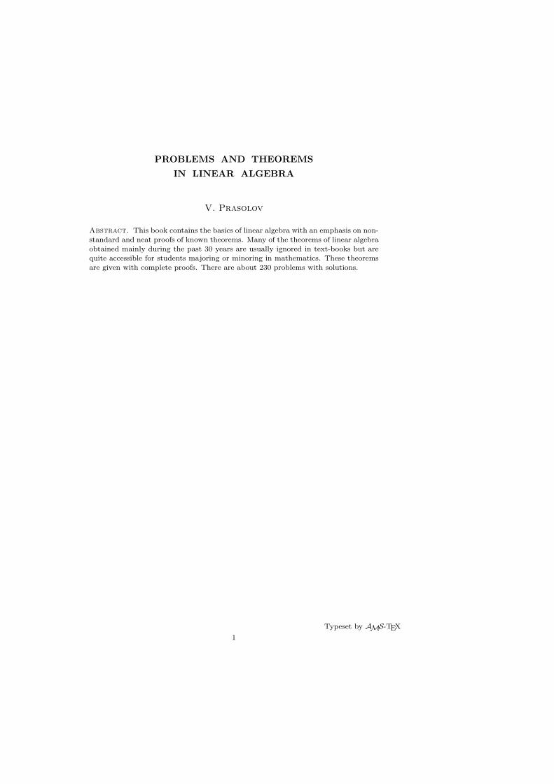
CONTENTS
PrefaceMain notations and conventionsChapter I. DeterminantsHistorical remarks: Leibniz and Seki Kova. Cramer, L’Hospital,
Cauchy and Jacobi1. Basic properties of determinants
The Vandermonde determinant and its application. The Cauchy deter-minant. Continued fractions and the determinant of a tridiagonal matrix.Certain other determinants.
Problems
2. Minors and cofactorsBinet-Cauchy’s formula. Laplace’s theorem. Jacobi’s theorem on minors
of the adjoint matrix. The generalized Sylvester’s identity. Chebotarev’s
theorem on the matrixřřεijřřp−1
1, where ε = exp(2πi/p).
Problems
3. The Schur complementGiven A =
ţA11 A12
A21 A22
ű, the matrix (A|A11) = A22 − A21A
−111 A12 is
called the Schur complement (of A11 in A).3.1. det A = det A11 det (A|A11).
3.2. Theorem. (A|B) = ((A|C)|(B|C)).
Problems
4. Symmetric functions, sums xk1+· · ·+xkn, and Bernoulli numbersDeterminant relations between σk(x1, . . . , xn), sk(x1, . . . , xn) = xk1 +· · ·+
xkn and pk(x1, . . . , xn) =P
i1+...ik=nxi11 . . . xinn . A determinant formula for
Sn(k) = 1n + · · ·+ (k − 1)n. The Bernoulli numbers and Sn(k).
4.4. Theorem. Let u = S1(x) and v = S2(x). Then for k ≥ 1 there exist
polynomials pk and qk such that S2k+1(x) = u2pk(u) and S2k(x) = vqk(u).
Problems
Solutions
Chapter II. Linear spacesHistorical remarks: Hamilton and Grassmann
5. The dual space. The orthogonal complementLinear equations and their application to the following theorem:5.4.3. Theorem. If a rectangle with sides a and b is arbitrarily cut into
squares with sides x1, . . . , xn thenxi
a∈ Q and
xi
b∈ Q for all i.
Typeset by AMS-TEX
1
2
Problems
6. The kernel (null space) and the image (range) of an operator.The quotient space6.2.1. Theorem. KerA∗ = (ImA)⊥ and ImA∗ = (KerA)⊥.
Fredholm’s alternative. Kronecker-Capelli’s theorem. Criteria for solv-ability of the matrix equation C = AXB.
Problem
7. Bases of a vector space. Linear independenceChange of basis. The characteristic polynomial.
7.2. Theorem. Let x1, . . . , xn and y1, . . . , yn be two bases, 1 ≤ k ≤ n.Then k of the vectors y1, . . . , yn can be interchanged with some k of thevectors x1, . . . , xn so that we get again two bases.
7.3. Theorem. Let T : V −→ V be a linear operator such that thevectors ξ, T ξ, . . . , Tnξ are linearly dependent for every ξ ∈ V . Then theoperators I, T, . . . , Tn are linearly dependent.
Problems
8. The rank of a matrixThe Frobenius inequality. The Sylvester inequality.
8.3. Theorem. Let U be a linear subspace of the space Mn,m of n×mmatrices, and r ≤ m ≤ n. If rankX ≤ r for any X ∈ U then dimU ≤ rn.
A description of subspaces U ⊂Mn,m such that dimU = nr.
Problems
9. Subspaces. The Gram-Schmidt orthogonalization processOrthogonal projections.
9.5. Theorem. Let e1, . . . , en be an orthogonal basis for a space V ,di =
řřeiřř. The projections of the vectors e1, . . . , en onto an m-dimensional
subspace of V have equal lengths if and only if d2i (d−21 + · · ·+ d−2
n ) ≥ m forevery i = 1, . . . , n.
9.6.1. Theorem. A set of k-dimensional subspaces of V is such thatany two of these subspaces have a common (k − 1)-dimensional subspace.Then either all these subspaces have a common (k−1)-dimensional subspaceor all of them are contained in the same (k + 1)-dimensional subspace.
Problems
10. Complexification and realification. Unitary spacesUnitary operators. Normal operators.
10.3.4. Theorem. Let B and C be Hermitian operators. Then theoperator A = B + iC is normal if and only if BC = CB.
Complex structures.
Problems
SolutionsChapter III. Canonical forms of matrices and linear op-
erators
11. The trace and eigenvalues of an operatorThe eigenvalues of an Hermitian operator and of a unitary operator. The
eigenvalues of a tridiagonal matrix.
Problems
12. The Jordan canonical (normal) form12.1. Theorem. If A and B are matrices with real entries and A =
PBP−1 for some matrix P with complex entries then A = QBQ−1 for somematrix Q with real entries.
CONTENTS 3
The existence and uniqueness of the Jordan canonical form (Valiacho’ssimple proof).
The real Jordan canonical form.
12.5.1. Theorem. a) For any operator A there exist a nilpotent operatorAn and a semisimple operator As such that A = As+An and AsAn = AnAs.
b) The operators An and As are unique; besides, As = S(A) and An =N(A) for some polynomials S and N .
12.5.2. Theorem. For any invertible operator A there exist a unipotentoperator Au and a semisimple operator As such that A = AsAu = AuAs.Such a representation is unique.
Problems
13. The minimal polynomial and the characteristic polynomial13.1.2. Theorem. For any operator A there exists a vector v such that
the minimal polynomial of v (with respect to A) coincides with the minimalpolynomial of A.
13.3. Theorem. The characteristic polynomial of a matrix A coincideswith its minimal polynomial if and only if for any vector (x1, . . . , xn) thereexist a column P and a row Q such that xk = QAkP .
Hamilton-Cayley’s theorem and its generalization for polynomials of ma-
trices.
Problems
14. The Frobenius canonical formExistence of Frobenius’s canonical form (H. G. Jacob’s simple proof)
Problems
15. How to reduce the diagonal to a convenient form15.1. Theorem. If A 6= λI then A is similar to a matrix with the
diagonal elements (0, . . . , 0, trA).
15.2. Theorem. Any matrix A is similar to a matrix with equal diagonalelements.
15.3. Theorem. Any nonzero square matrix A is similar to a matrix
all diagonal elements of which are nonzero.
Problems
16. The polar decompositionThe polar decomposition of noninvertible and of invertible matrices. The
uniqueness of the polar decomposition of an invertible matrix.
16.1. Theorem. If A = S1U1 = U2S2 are polar decompositions of aninvertible matrix A then U1 = U2.
16.2.1. Theorem. For any matrix A there exist unitary matrices U,Wand a diagonal matrix D such that A = UDW .
Problems
17. Factorizations of matrices17.1. Theorem. For any complex matrix A there exist a unitary matrix
U and a triangular matrix T such that A = UTU∗. The matrix A is anormal one if and only if T is a diagonal one.
Gauss’, Gram’s, and Lanczos’ factorizations.
17.3. Theorem. Any matrix is a product of two symmetric matrices.
Problems
18. Smith’s normal form. Elementary factors of matricesProblems
Solutions
4
Chapter IV. Matrices of special form
19. Symmetric and Hermitian matricesSylvester’s criterion. Sylvester’s law of inertia. Lagrange’s theorem on
quadratic forms. Courant-Fisher’s theorem.
19.5.1.Theorem. If A ≥ 0 and (Ax, x) = 0 for any x, then A = 0.
Problems
20. Simultaneous diagonalization of a pair of Hermitian formsSimultaneous diagonalization of two Hermitian matrices A and B when
A > 0. An example of two Hermitian matrices which can not be simultane-ously diagonalized. Simultaneous diagonalization of two semidefinite matri-ces. Simultaneous diagonalization of two Hermitian matrices A and B suchthat there is no x 6= 0 for which x∗Ax = x∗Bx = 0.
Problems
§21. Skew-symmetric matrices21.1.1. Theorem. If A is a skew-symmetric matrix then A2 ≤ 0.
21.1.2. Theorem. If A is a real matrix such that (Ax, x) = 0 for all x,then A is a skew-symmetric matrix.
21.2. Theorem. Any skew-symmetric bilinear form can be expressed asrPk=1
(x2k−1y2k − x2ky2k−1).
Problems
22. Orthogonal matrices. The Cayley transformationThe standard Cayley transformation of an orthogonal matrix which does
not have 1 as its eigenvalue. The generalized Cayley transformation of anorthogonal matrix which has 1 as its eigenvalue.
Problems
23. Normal matrices23.1.1. Theorem. If an operator A is normal then KerA∗ = KerA and
ImA∗ = ImA.
23.1.2. Theorem. An operator A is normal if and only if any eigen-vector of A is an eigenvector of A∗.
23.2. Theorem. If an operator A is normal then there exists a polyno-mial P such that A∗ = P (A).
Problems
24. Nilpotent matrices24.2.1. Theorem. Let A be an n×n matrix. The matrix A is nilpotent
if and only if tr (Ap) = 0 for each p = 1, . . . , n.
Nilpotent matrices and Young tableaux.
Problems
25. Projections. Idempotent matrices25.2.1&2. Theorem. An idempotent operator P is an Hermitian one
if and only if a) KerP ⊥ ImP ; or b) |Px| ≤ |x| for every x.
25.2.3. Theorem. Let P1, . . . , Pn be Hermitian, idempotent operators.The operator P = P1 + · · ·+Pn is an idempotent one if and only if PiPj = 0whenever i 6= j.
25.4.1. Theorem. Let V1 ⊕ · · · ⊕ Vk, Pi : V −→ Vi be Hermitian
idempotent operators, A = P1 + · · ·+Pk. Then 0 < det A ≤ 1 and det A = 1
if and only if Vi ⊥ Vj whenever i 6= j.
Problems
26. Involutions
CONTENTS 5
26.2. Theorem. A matrix A can be represented as the product of two
involutions if and only if the matrices A and A−1 are similar.
Problems
Solutions
Chapter V. Multilinear algebra
27. Multilinear maps and tensor productsAn invariant definition of the trace. Kronecker’s product of matrices,
A ⊗ B; the eigenvalues of the matrices A ⊗ B and A ⊗ I + I ⊗ B. Matrix
equations AX −XB = C and AX −XB = λX.
Problems
28. Symmetric and skew-symmetric tensorsThe Grassmann algebra. Certain canonical isomorphisms. Applications
of Grassmann algebra: proofs of Binet-Cauchy’s formula and Sylvester’s iden-tity.
28.5.4. Theorem. Let ΛB(t) = 1 +nPq=1
tr(ΛqB)tq and SB(t) = 1 +
nPq=1
tr (SqB)tq. Then SB(t) = (ΛB(−t))−1.
Problems
29. The PfaffianThe Pfaffian of principal submatrices of the matrix M =
řřmijřř2n
1, where
mij = (−1)i+j+1.
29.2.2. Theorem. Given a skew-symmetric matrix A we have
Pf (A+ λ2M) =nX
k=0
λ2kpk, where pk =Xσ
A
Ãσ1 . . . σ2(n−k)
σ1 . . . σ2(n−k)
!
Problems
30. Decomposable skew-symmetric and symmetric tensors30.1.1. Theorem. x1 ∧ · · · ∧ xk = y1 ∧ · · · ∧ yk 6= 0 if and only if
Span(x1, . . . , xk) = Span(y1, . . . , yk).
30.1.2. Theorem. S(x1 ⊗ · · · ⊗ xk) = S(y1 ⊗ · · · ⊗ yk) 6= 0 if and onlyif Span(x1, . . . , xk) = Span(y1, . . . , yk).
Plucker relations.
Problems
31. The tensor rankStrassen’s algorithm. The set of all tensors of rank ≤ 2 is not closed. The
rank over R is not equal, generally, to the rank over C.
Problems
32. Linear transformations of tensor productsA complete description of the following types of transformations of
Vm ⊗ (V ∗)n ∼= Mm,n :
1) rank-preserving;
2) determinant-preserving;
3) eigenvalue-preserving;
4) invertibility-preserving.
6
Problems
SolutionsChapter VI. Matrix inequalities
33. Inequalities for symmetric and Hermitian matrices33.1.1. Theorem. If A > B > 0 then A−1 < B−1.33.1.3. Theorem. If A > 0 is a real matrix then
(A−1x, x) = maxy
(2(x, y)− (Ay, y)).
33.2.1. Theorem. Suppose A =
ţA1 BB∗ A2
ű> 0. Then |A| ≤ |A1| ·
|A2|.Hadamard’s inequality and Szasz’s inequality.
33.3.1. Theorem. Suppose αi > 0,nPi=1
αi = 1 and Ai > 0. Then
|α1A1 + · · ·+ αkAk| ≥ |A1|α1 + · · ·+ |Ak|αk .
33.3.2. Theorem. Suppose Ai ≥ 0, αi ∈ C. Then
|det(α1A1 + · · ·+ αkAk)| ≤ det(|α1|A1 + · · ·+ |αk|Ak).
Problems
34. Inequalities for eigenvaluesSchur’s inequality. Weyl’s inequality (for eigenvalues of A+B).
34.2.2. Theorem. Let A =
ţB CC∗ B
ű> 0 be an Hermitian matrix,
α1 ≤ · · · ≤ αn and β1 ≤ · · · ≤ βm the eigenvalues of A and B, respectively.Then αi ≤ βi ≤ αn+i−m.
34.3. Theorem. Let A and B be Hermitian idempotents, λ any eigen-value of AB. Then 0 ≤ λ ≤ 1.
34.4.1. Theorem. Let the λi and µi be the eigenvalues of A and AA∗,respectively; let σi =
√µi. Let |λ1 ≤ · · · ≤ λn, where n is the order of A.
Then |λ1 . . . λm| ≤ σ1 . . . σm.34.4.2.Theorem. Let σ1 ≥ · · · ≥ σn and τ1 ≥ · · · ≥ τn be the singular
values of A and B. Then | tr (AB)| ≤Pσiτi.
Problems
35. Inequalities for matrix normsThe spectral norm ‖A‖s and the Euclidean norm ‖A‖e, the spectral radius
ρ(A).35.1.2. Theorem. If a matrix A is normal then ρ(A) = ‖A‖s.35.2. Theorem. ‖A‖s ≤ ‖A‖e ≤
√n‖A‖s.
The invariance of the matrix norm and singular values.
35.3.1. Theorem. Let S be an Hermitian matrix. Then ‖A− A+A∗
2‖
does not exceed ‖A− S‖, where ‖·‖ is the Euclidean or operator norm.35.3.2. Theorem. Let A = US be the polar decomposition of A and
W a unitary matrix. Then ‖A− U‖e ≤ ‖A−W‖e and if |A| 6= 0, then theequality is only attained for W = U .
Problems
36. Schur’s complement and Hadamard’s product. Theorems ofEmily Haynsworth
CONTENTS 7
36.1.1. Theorem. If A > 0 then (A|A11) > 0.36.1.4. Theorem. If Ak and Bk are the k-th principal submatrices of
positive definite order n matrices A and B, then
|A+B| ≥ |A|Ã
1 +
n−1X
k=1
|Bk||Ak|
!+ |B|
Ã1 +
n−1X
k=1
|Ak||Bk|
!.
Hadamard’s product A B.36.2.1. Theorem. If A > 0 and B > 0 then A B > 0.Oppenheim’s inequality
Problems
37. Nonnegative matricesWielandt’s theorem
Problems
38. Doubly stochastic matricesBirkhoff’s theorem. H.Weyl’s inequality.
SolutionsChapter VII. Matrices in algebra and calculus
39. Commuting matricesThe space of solutions of the equation AX = XA for X with the given A
of order n.39.2.2. Theorem. Any set of commuting diagonalizable operators has
a common eigenbasis.39.3. Theorem. Let A,B be matrices such that AX = XA implies
BX = XB. Then B = g(A), where g is a polynomial.
Problems
40. Commutators40.2. Theorem. If trA = 0 then there exist matrices X and Y such
that [X,Y ] = A and either (1) trY = 0 and an Hermitian matrix X or (2)X and Y have prescribed eigenvalues.
40.3. Theorem. Let A,B be matrices such that adsAX = 0 impliesadsX B = 0 for some s > 0. Then B = g(A) for a polynomial g.
40.4. Theorem. Matrices A1, . . . , An can be simultaneously triangular-ized over C if and only if the matrix p(A1, . . . , An)[Ai, Aj ] is a nilpotent onefor any polynomial p(x1, . . . , xn) in noncommuting indeterminates.
40.5. Theorem. If rank[A,B] ≤ 1, then A and B can be simultaneouslytriangularized over C.
Problems
41. Quaternions and Cayley numbers. Clifford algebrasIsomorphisms so(3,R) ∼= su(2) and so(4,R) ∼= so(3,R) ⊕ so(3,R). The
vector products in R3 and R7. Hurwitz-Radon families of matrices. Hurwitz-Radon’ number ρ(2c+4d(2a+ 1)) = 2c + 8d.
41.7.1. Theorem. The identity of the form
(x21 + · · ·+ x2
n)(y21 + · · ·+ y2
n) = (z21 + · · ·+ z2
n),
where zi(x, y) is a bilinear function, holds if and only if m ≤ ρ(n).41.7.5. Theorem. In the space of real n × n matrices, a subspace of
invertible matrices of dimension m exists if and only if m ≤ ρ(n).Other applications: algebras with norm, vector product, linear vector
fields on spheres.Clifford algebras and Clifford modules.
8
Problems
42. Representations of matrix algebrasComplete reducibility of finite-dimensional representations of Mat(V n).
Problems
43. The resultantSylvester’s matrix, Bezout’s matrix and Barnett’s matrix
Problems
44. The general inverse matrix. Matrix equations44.3. Theorem. a) The equation AX −XA = C is solvable if and only
if the matrices
ţA OO B
űand
ţA CO B
űare similar.
b) The equation AX − Y A = C is solvable if and only if rank
ţA OO B
ű
= rank
ţA CO B
ű.
Problems
45. Hankel matrices and rational functions
46. Functions of matrices. Differentiation of matricesDifferential equation X = AX and the Jacobi formula for det A.
Problems
47. Lax pairs and integrable systems
48. Matrices with prescribed eigenvalues48.1.2. Theorem. For any polynomial f(x) = xn+c1xn−1+· · ·+cn and
any matrix B of order n− 1 whose characteristic and minimal polynomialscoincide there exists a matrix A such that B is a submatrix of A and thecharacteristic polynomial of A is equal to f .
48.2. Theorem. Given all offdiagonal elements in a complex matrix Ait is possible to select diagonal elements x1, . . . , xn so that the eigenvaluesof A are given complex numbers; there are finitely many sets x1, . . . , xnsatisfying this condition.
Solutions
AppendixEisenstein’s criterion, Hilbert’s Nullstellensats.
Bibliography
Index
CONTENTS 9
PREFACE
There are very many books on linear algebra, among them many really wonderfulones (see e.g. the list of recommended literature). One might think that one doesnot need any more books on this subject. Choosing one’s words more carefully, itis possible to deduce that these books contain all that one needs and in the bestpossible form, and therefore any new book will, at best, only repeat the old ones.
This opinion is manifestly wrong, but nevertheless almost ubiquitous.New results in linear algebra appear constantly and so do new, simpler and
neater proofs of the known theorems. Besides, more than a few interesting oldresults are ignored, so far, by text-books.
In this book I tried to collect the most attractive problems and theorems of linearalgebra still accessible to first year students majoring or minoring in mathematics.
The computational algebra was left somewhat aside. The major part of the bookcontains results known from journal publications only. I believe that they will beof interest to many readers.
I assume that the reader is acquainted with main notions of linear algebra:linear space, basis, linear map, the determinant of a matrix. Apart from that,all the essential theorems of the standard course of linear algebra are given herewith complete proofs and some definitions from the above list of prerequisites isrecollected. I made the prime emphasis on nonstandard neat proofs of knowntheorems.
In this book I only consider finite dimensional linear spaces.The exposition is mostly performed over the fields of real or complex numbers.
The peculiarity of the fields of finite characteristics is mentioned when needed.Cross-references inside the book are natural: 36.2 means subsection 2 of sec. 36;
Problem 36.2 is Problem 2 from sec. 36; Theorem 36.2.2 stands for Theorem 2from 36.2.
Acknowledgments. The book is based on a course I read at the IndependentUniversity of Moscow, 1991/92. I am thankful to the participants for comments andto D. V. Beklemishev, D. B. Fuchs, A. I. Kostrikin, V. S. Retakh, A. N. Rudakovand A. P. Veselov for fruitful discussions of the manuscript.
Typeset by AMS-TEX

10 PREFACE
Main notations and conventions
A =
a11 . . . a1n
. . . . . . . . .am1 . . . amn
denotes a matrix of size m × n; we say that a square
n× n matrix is of order n;aij , sometimes denoted by ai,j for clarity, is the element or the entry from the
intersection of the i-th row and the j-th column;(aij) is another notation for the matrix A;∥∥aij
∥∥np
still another notation for the matrix (aij), where p ≤ i, j ≤ n;det(A), |A| and det(aij) all denote the determinant of the matrix A;|aij |np is the determinant of the matrix
∥∥aij∥∥np;
Eij — the (i, j)-th matrix unit — the matrix whose only nonzero element isequal to 1 and occupies the (i, j)-th position;AB — the product of a matrix A of size p × n by a matrix B of size n × q —
is the matrix (cij) of size p× q, where cik =n∑j=1
aijbjk, is the scalar product of the
i-th row of the matrix A by the k-th column of the matrix B;diag(λ1, . . . , λn) is the diagonal matrix of size n× n with elements aii = λi and
zero offdiagonal elements;I = diag(1, . . . , 1) is the unit matrix; when its size, n×n, is needed explicitly we
denote the matrix by In;the matrix aI, where a is a number, is called a scalar matrix;AT is the transposed of A, AT = (a′ij), where a′ij = aji;A = (a′ij), where a′ij = aij ;
A∗ = AT ;σ =
(1 ... nk1 ...kn
)is a permutation: σ(i) = ki; the permutation
(1 ... nk1 ...kn
)is often
abbreviated to (k1 . . . kn);
sign σ = (−1)σ =
1 if σ is even−1 if σ is odd
;
Span(e1, . . . , en) is the linear space spanned by the vectors e1, . . . , en;Given bases e1, . . . , en and εεε1, . . . , εεεm in spaces V n and Wm, respectively, we
assign to a matrix A the operator A : V n −→ Wm which sends the vector
x1...xn
into the vector
y1...ym
=
a11 . . . a1n... . . .
...am1 . . . amn
x1...xn
.
Since yi =n∑j=1
aijxj , then
A(n∑
j=1
xjej) =m∑
i=1
n∑
j=1
aijxjεεεi;
in particular, Aej =∑i
aijεεεi;
in the whole book except for §37 the notation
MAIN NOTATIONS AND CONVENTIONS 11
A > 0, A ≥ 0, A < 0 or A ≤ 0 denote that a real symmetric or Hermitian matrixA is positive definite, nonnegative definite, negative definite or nonpositive definite,respectively; A > B means that A−B > 0; whereas in §37 they mean that aij > 0for all i, j, etc.
CardM is the cardinality of the set M , i.e, the number of elements of M ;A|W denotes the restriction of the operator A : V −→ V onto the subspace
W ⊂ V ;sup the least upper bound (supremum);Z,Q,R,C,H,O denote, as usual, the sets of all integer, rational, real, complex,
quaternion and octonion numbers, respectively;N denotes the set of all positive integers (without 0);
δij =
1 if i = j,
0 otherwise.
12 PREFACECHAPTER I
DETERMINANTS
The notion of a determinant appeared at the end of 17th century in works ofLeibniz (1646–1716) and a Japanese mathematician, Seki Kova, also known asTakakazu (1642–1708). Leibniz did not publish the results of his studies relatedwith determinants. The best known is his letter to l’Hospital (1693) in whichLeibniz writes down the determinant condition of compatibility for a system of threelinear equations in two unknowns. Leibniz particularly emphasized the usefulnessof two indices when expressing the coefficients of the equations. In modern termshe actually wrote about the indices i, j in the expression xi =
∑j aijyj .
Seki arrived at the notion of a determinant while solving the problem of findingcommon roots of algebraic equations.
In Europe, the search for common roots of algebraic equations soon also becamethe main trend associated with determinants. Newton, Bezout, and Euler studiedthis problem.
Seki did not have the general notion of the derivative at his disposal, but heactually got an algebraic expression equivalent to the derivative of a polynomial.He searched for multiple roots of a polynomial f(x) as common roots of f(x) andf ′(x). To find common roots of polynomials f(x) and g(x) (for f and g of smalldegrees) Seki got determinant expressions. The main treatise by Seki was publishedin 1674; there applications of the method are published, rather than the methoditself. He kept the main method in secret confiding only in his closest pupils.
In Europe, the first publication related to determinants, due to Cramer, ap-peared in 1750. In this work Cramer gave a determinant expression for a solutionof the problem of finding the conic through 5 fixed points (this problem reduces toa system of linear equations).
The general theorems on determinants were proved only ad hoc when needed tosolve some other problem. Therefore, the theory of determinants had been develop-ing slowly, left behind out of proportion as compared with the general developmentof mathematics. A systematic presentation of the theory of determinants is mainlyassociated with the names of Cauchy (1789–1857) and Jacobi (1804–1851).
1. Basic properties of determinants
The determinant of a square matrix A =∥∥aij
∥∥n1
is the alternated sum
∑σ
(−1)σa1σ(1)a2σ(2) . . . anσ(n),
where the summation is over all permutations σ ∈ Sn. The determinant of thematrix A =
∥∥aij∥∥n
1is denoted by detA or |aij |n1 . If detA 6= 0, then A is called
invertible or nonsingular.The following properties are often used to compute determinants. The reader
can easily verify (or recall) them.1. Under the permutation of two rows of a matrix A its determinant changes
the sign. In particular, if two rows of the matrix are identical, detA = 0.
Typeset by AMS-TEX
1. BASIC PROPERTIES OF DETERMINANTS 13
2. If A and B are square matrices, det(A C0 B
)= detA · detB.
3. |aij |n1 =∑nj=1(−1)i+jaijMij , where Mij is the determinant of the matrix
obtained from A by crossing out the ith row and the jth column of A (the row(echelon) expansion of the determinant or, more precisely, the expansion with respectto the ith row).
(To prove this formula one has to group the factors of aij , where j = 1, . . . , n,for a fixed i.)
4.∣∣∣∣∣∣∣
λα1 + µβ1 a12 . . . a1n...
... · · · ...λαn + µβn an2 . . . ann
∣∣∣∣∣∣∣= λ
∣∣∣∣∣∣
α1 a12 . . . a1n...
... · · · ...αn an2 . . . ann
∣∣∣∣∣∣+µ
∣∣∣∣∣∣∣
β1 a12 . . . a1n...
... · · · ...βn an2 . . . ann
∣∣∣∣∣∣∣.
5. det(AB) = detAdetB.6. det(AT ) = detA.
1.1. Before we start computing determinants, let us prove Cramer’s rule. Itappeared already in the first published paper on determinants.
Theorem (Cramer’s rule). Consider a system of linear equations
x1ai1 + · · ·+ xnain = bi (i = 1, . . . , n),
i.e.,x1A1 + · · ·+ xnAn = B,
where Aj is the jth column of the matrix A =∥∥aij
∥∥n1
. Then
xi det(A1, . . . , An) = det (A1, . . . , B, . . . , An) ,
where the column B is inserted instead of Ai.
Proof. Since for j 6= i the determinant of the matrix det(A1, . . . , Aj , . . . , An),a matrix with two identical columns, vanishes,
det(A1, . . . , B, . . . , An) = det (A1, . . . ,∑xjAj , . . . , An)
=∑
xj det(A1, . . . , Aj , . . . , An) = xi det(A1, . . . , An). ¤
If det(A1, . . . , An) 6= 0 the formula obtained can be used to find solutions of asystem of linear equations.
1.2. One of the most often encountered determinants is the Vandermonde de-terminant, i.e., the determinant of the Vandermonde matrix
V (x1, . . . , xn) =
∣∣∣∣∣∣∣
1 x1 x21 . . . xn−1
1...
...... · · · ...
1 xn x2n . . . xn−1
n
∣∣∣∣∣∣∣=
∏
i>j
(xi − xj).
To compute this determinant, let us subtract the (k − 1)-st column multipliedby x1 from the kth one for k = n, n − 1, . . . , 2. The first row takes the form
14 DETERMINANTS
(1, 0, 0, . . . , 0), i.e., the computation of the Vandermonde determinant of order nreduces to a determinant of order n−1. Factorizing each row of the new determinantby bringing out xi − x1 we get
V (x1, . . . , xn) =∏
i>1
(xi − x1)
∣∣∣∣∣∣∣
1 x2 x22 . . . xn−2
1...
...... · · · ...
1 xn x2n . . . xn−2
n
∣∣∣∣∣∣∣.
For n = 2 the identity V (x1, x2) = x2 − x1 is obvious, hence,
V (x1, . . . , xn) =∏
i>j
(xi − xj).
Many of the applications of the Vandermonde determinant are occasioned bythe fact that V (x1, . . . , xn) = 0 if and only if there are two equal numbers amongx1, . . . , xn.
1.3. The Cauchy determinant |aij |n1 , where aij = (xi + yj)−1, is slightly moredifficult to compute than the Vandermonde determinant.
Let us prove by induction that
|aij |n1 =
∏i>j
(xi − xj)(yi − yj)∏i,j
(xi + yj).
For a base of induction take |aij |11 = (x1 + y1)−1.The step of induction will be performed in two stages.First, let us subtract the last column from each of the preceding ones. We get
a′ij = (xi + yj)−1 − (xi + yn)−1 = (yn − yj)(xi + yn)−1(xi + yj)−1 for j 6= n.
Let us take out of each row the factors (xi + yn)−1 and take out of each column,except the last one, the factors yn − yj . As a result we get the determinant |bij |n1 ,where bij = aij for j 6= n and bin = 1.
To compute this determinant, let us subtract the last row from each of thepreceding ones. Taking out of each row, except the last one, the factors xn − xiand out of each column, except the last one, the factors (xn + yj)−1 we make itpossible to pass to a Cauchy determinant of lesser size.
1.4. A matrix A of the form
0 1 0 . . . 0 00 0 1 . . . 0 0...
.... . . . . . . . .
...
0 0 0. . . 1 0
0 0 0 . . . 0 1a0 a1 a2 . . . an−2 an−1
is called Frobenius’ matrix or the companion matrix of the polynomial
p(λ) = λn − an−1λn−1 − an−2λ
n−2 − · · · − a0.
With the help of the expansion with respect to the first row it is easy to verify byinduction that
det(λI −A) = λn − an−1λn−1 − an−2λ
n−2 − · · · − a0 = p(λ).
1. BASIC PROPERTIES OF DETERMINANTS 15
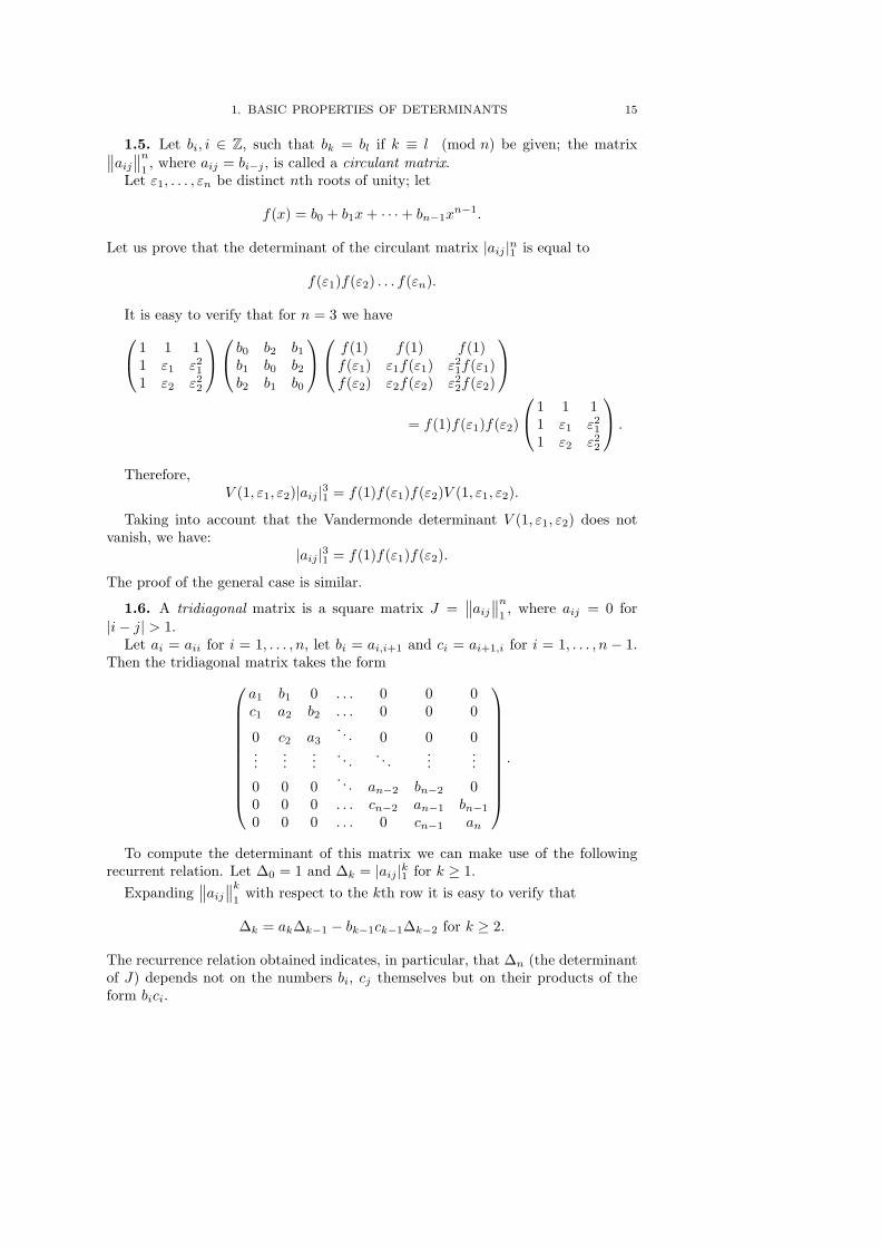
1.5. Let bi, i ∈ Z, such that bk = bl if k ≡ l (mod n) be given; the matrix∥∥aij∥∥n
1, where aij = bi−j , is called a circulant matrix.
Let ε1, . . . , εn be distinct nth roots of unity; let
f(x) = b0 + b1x+ · · ·+ bn−1xn−1.
Let us prove that the determinant of the circulant matrix |aij |n1 is equal to
f(ε1)f(ε2) . . . f(εn).
It is easy to verify that for n = 3 we have
1 1 11 ε1 ε2
1
1 ε2 ε22
b0 b2 b1b1 b0 b2b2 b1 b0
f(1) f(1) f(1)f(ε1) ε1f(ε1) ε2
1f(ε1)f(ε2) ε2f(ε2) ε2
2f(ε2)
= f(1)f(ε1)f(ε2)
1 1 11 ε1 ε2
1
1 ε2 ε22
.
Therefore,V (1, ε1, ε2)|aij |31 = f(1)f(ε1)f(ε2)V (1, ε1, ε2).
Taking into account that the Vandermonde determinant V (1, ε1, ε2) does notvanish, we have:
|aij |31 = f(1)f(ε1)f(ε2).
The proof of the general case is similar.
1.6. A tridiagonal matrix is a square matrix J =∥∥aij
∥∥n1, where aij = 0 for
|i− j| > 1.Let ai = aii for i = 1, . . . , n, let bi = ai,i+1 and ci = ai+1,i for i = 1, . . . , n − 1.
Then the tridiagonal matrix takes the form
a1 b1 0 . . . 0 0 0c1 a2 b2 . . . 0 0 0
0 c2 a3. . . 0 0 0
......
.... . . . . .
......
0 0 0. . . an−2 bn−2 0
0 0 0 . . . cn−2 an−1 bn−1
0 0 0 . . . 0 cn−1 an
.
To compute the determinant of this matrix we can make use of the followingrecurrent relation. Let ∆0 = 1 and ∆k = |aij |k1 for k ≥ 1.
Expanding∥∥aij
∥∥k1
with respect to the kth row it is easy to verify that
∆k = ak∆k−1 − bk−1ck−1∆k−2 for k ≥ 2.
The recurrence relation obtained indicates, in particular, that ∆n (the determinantof J) depends not on the numbers bi, cj themselves but on their products of theform bici.
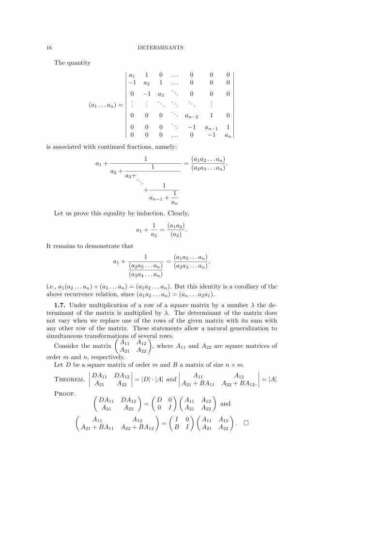
16 DETERMINANTS
The quantity
(a1 . . . an) =
∣∣∣∣∣∣∣∣∣∣∣∣∣∣∣∣∣
a1 1 0 . . . 0 0 0−1 a2 1 . . . 0 0 0
0 −1 a3. . . 0 0 0
......
. . . . . . . . ....
0 0 0. . . an−2 1 0
0 0 0. . . −1 an−1 1
0 0 0 . . . 0 −1 an
∣∣∣∣∣∣∣∣∣∣∣∣∣∣∣∣∣
is associated with continued fractions, namely:
a1 +1
a2 +1
a3+...+
1
an−1 +1an
=(a1a2 . . . an)(a2a3 . . . an)
.
Let us prove this equality by induction. Clearly,
a1 +1a2
=(a1a2)(a2)
.
It remains to demonstrate that
a1 +1
(a2a3 . . . an)(a3a4 . . . an)
=(a1a2 . . . an)(a2a3 . . . an)
,
i.e., a1(a2 . . . an) + (a3 . . . an) = (a1a2 . . . an). But this identity is a corollary of theabove recurrence relation, since (a1a2 . . . an) = (an . . . a2a1).
1.7. Under multiplication of a row of a square matrix by a number λ the de-terminant of the matrix is multiplied by λ. The determinant of the matrix doesnot vary when we replace one of the rows of the given matrix with its sum withany other row of the matrix. These statements allow a natural generalization tosimultaneous transformations of several rows.
Consider the matrix(A11 A12
A21 A22
), where A11 and A22 are square matrices of
order m and n, respectively.Let D be a square matrix of order m and B a matrix of size n×m.
Theorem.
∣∣∣∣DA11 DA12
A21 A22
∣∣∣∣ = |D| · |A| and∣∣∣∣
A11 A12
A21 +BA11 A22 +BA12.
∣∣∣∣ = |A|
Proof. (DA11 DA12
A21 A22
)=
(D 00 I
)(A11 A12
A21 A22
)and
(A11 A12
A21 +BA11 A22 +BA12
)=
(I 0B I
) (A11 A12
A21 A22
). ¤

1. BASIC PROPERTIES OF DETERMINANTS 17
Problems
1.1. Let A =∥∥aij
∥∥n1
be skew-symmetric, i.e., aij = −aji, and let n be odd.Prove that |A| = 0.
1.2. Prove that the determinant of a skew-symmetric matrix of even order doesnot change if to all its elements we add the same number.
1.3. Compute the determinant of a skew-symmetric matrix An of order 2n witheach element above the main diagonal being equal to 1.
1.4. Prove that for n ≥ 3 the terms in the expansion of a determinant of ordern cannot be all positive.
1.5. Let aij = a|i−j|. Compute |aij |n1 .
1.6. Let ∆3 =
∣∣∣∣∣∣∣
1 −1 0 0x h −1 0x2 hx h −1x3 hx2 hx h
∣∣∣∣∣∣∣and define ∆n accordingly. Prove that
∆n = (x+ h)n.1.7. Compute |cij |n1 , where cij = aibj for i 6= j and cii = xi.1.8. Let ai,i+1 = ci for i = 1, . . . , n, the other matrix elements being zero. Prove
that the determinant of the matrix I +A+A2 + · · ·+An−1 is equal to (1− c)n−1,where c = c1 . . . cn.
1.9. Compute |aij |n1 , where aij = (1− xiyj)−1.1.10. Let aij =
(n+ij
). Prove that |aij |m0 = 1.
1.11. Prove that for any real numbers a, b, c, d, e and f
∣∣∣∣∣∣
(a+ b)de− (d+ e)ab ab− de a+ b− d− e(b+ c)ef − (e+ f)bc bc− ef b+ c− e− f(c+ d)fa− (f + a)cd cd− fa c+ d− f − a
∣∣∣∣∣∣= 0.
Vandermonde’s determinant.1.12. Compute
∣∣∣∣∣∣∣
1 x1 . . . xn−21 (x2 + x3 + · · ·+ xn)n−1
...... · · · ...
...1 xn . . . xn−2
n (x1 + x2 + · · ·+ xn−1)n−1
∣∣∣∣∣∣∣.
1.13. Compute ∣∣∣∣∣∣∣
1 x1 . . . xn−21 x2x3 . . . xn
...... · · · ...
...1 xn . . . xn−2
n x1x2 . . . xn−1
∣∣∣∣∣∣∣.
1.14. Compute |aik|n0 , where aik = λn−ki (1 + λ2i )k.
1.15. Let V =∥∥aij
∥∥n0, where aij = xj−1
i , be a Vandermonde matrix; let Vk bethe matrix obtained from V by deleting its (k+ 1)st column (which consists of thekth powers) and adding instead the nth column consisting of the nth powers. Provethat
detVk = σn−k(x1, . . . , xn) detV.
1.16. Let aij =(inj
). Prove that |aij |r1 = nr(r+1)/2 for r ≤ n.
18 DETERMINANTS
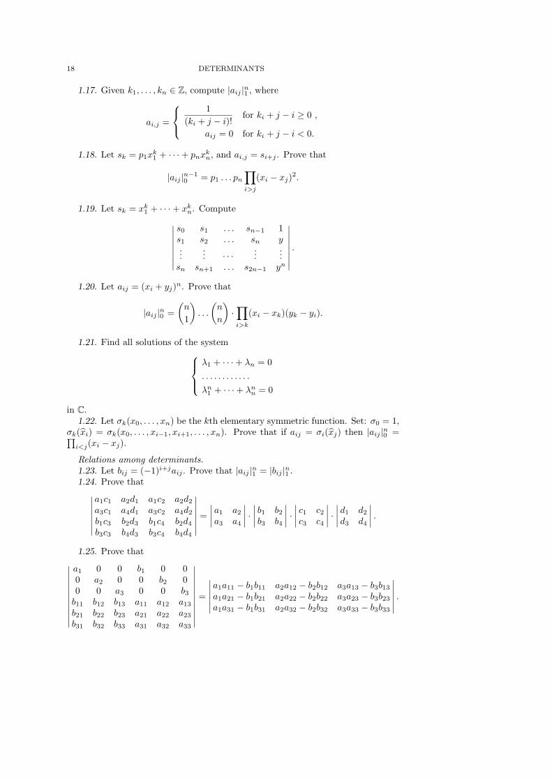
1.17. Given k1, . . . , kn ∈ Z, compute |aij |n1 , where
ai,j =
1(ki + j − i)! for ki + j − i ≥ 0 ,
aij = 0 for ki + j − i < 0.
1.18. Let sk = p1xk1 + · · ·+ pnx
kn, and ai,j = si+j . Prove that
|aij |n−10 = p1 . . . pn
∏
i>j
(xi − xj)2.
1.19. Let sk = xk1 + · · ·+ xkn. Compute
∣∣∣∣∣∣∣∣
s0 s1 . . . sn−1 1s1 s2 . . . sn y...
... · · · ......
sn sn+1 . . . s2n−1 yn
∣∣∣∣∣∣∣∣.
1.20. Let aij = (xi + yj)n. Prove that
|aij |n0 =(n
1
). . .
(n
n
)·∏
i>k
(xi − xk)(yk − yi).
1.21. Find all solutions of the system
λ1 + · · ·+ λn = 0. . . . . . . . . . . .
λn1 + · · ·+ λnn = 0
in C.1.22. Let σk(x0, . . . , xn) be the kth elementary symmetric function. Set: σ0 = 1,
σk(xi) = σk(x0, . . . , xi−1, xi+1, . . . , xn). Prove that if aij = σi(xj) then |aij |n0 =∏i<j(xi − xj).Relations among determinants.1.23. Let bij = (−1)i+jaij . Prove that |aij |n1 = |bij |n1 .1.24. Prove that
∣∣∣∣∣∣∣
a1c1 a2d1 a1c2 a2d2
a3c1 a4d1 a3c2 a4d2
b1c3 b2d3 b1c4 b2d4
b3c3 b4d3 b3c4 b4d4
∣∣∣∣∣∣∣=
∣∣∣∣a1 a2
a3 a4
∣∣∣∣ ·∣∣∣∣b1 b2b3 b4
∣∣∣∣ ·∣∣∣∣c1 c2c3 c4
∣∣∣∣ ·∣∣∣∣d1 d2
d3 d4
∣∣∣∣ .
1.25. Prove that∣∣∣∣∣∣∣∣∣∣∣
a1 0 0 b1 0 00 a2 0 0 b2 00 0 a3 0 0 b3b11 b12 b13 a11 a12 a13
b21 b22 b23 a21 a22 a23
b31 b32 b33 a31 a32 a33
∣∣∣∣∣∣∣∣∣∣∣
=
∣∣∣∣∣∣
a1a11 − b1b11 a2a12 − b2b12 a3a13 − b3b13
a1a21 − b1b21 a2a22 − b2b22 a3a23 − b3b23
a1a31 − b1b31 a2a32 − b2b32 a3a33 − b3b33
∣∣∣∣∣∣.
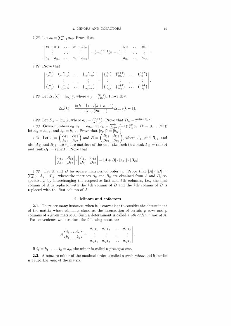
2. MINORS AND COFACTORS 19
1.26. Let sk =∑ni=1 aki. Prove that
∣∣∣∣∣∣
s1 − a11 . . . s1 − a1n... · · · ...
sn − an1 . . . sn − ann
∣∣∣∣∣∣= (−1)n−1(n− 1)
∣∣∣∣∣∣
a11 . . . a1n... · · · ...an1 . . . ann
∣∣∣∣∣∣.
1.27. Prove that∣∣∣∣∣∣∣
(nm1
) (n
m1−1
). . .
(n
m1−k)
...... · · · ...(
nmk
) (n
mk−1
). . .
(n
mk−k)
∣∣∣∣∣∣∣=
∣∣∣∣∣∣∣
(nm1
) (n+1m1
). . .
(n+km1
)...
... · · · ...(nmk
) (n+1mk
). . .
(n+kmk
)
∣∣∣∣∣∣∣.
1.28. Let ∆n(k) = |aij |n0 , where aij =(k+i2j
). Prove that
∆n(k) =k(k + 1) . . . (k + n− 1)
1 · 3 . . . (2n− 1)∆n−1(k − 1).
1.29. Let Dn = |aij |n0 , where aij =(n+i2j−1
). Prove that Dn = 2n(n+1)/2.
1.30. Given numbers a0, a1, ..., a2n, let bk =∑ki=0(−1)i
(ki
)ai (k = 0, . . . , 2n);
let aij = ai+j , and bij = bi+j . Prove that |aij |n0 = |bij |n0 .
1.31. Let A =(A11 A12
A21 A22
)and B =
(B11 B12
B21 B22
), where A11 and B11, and
also A22 and B22, are square matrices of the same size such that rankA11 = rankAand rankB11 = rankB. Prove that
∣∣∣∣A11 B12
A21 B22
∣∣∣∣ ·∣∣∣∣A11 A12
B21 B22
∣∣∣∣ = |A+B| · |A11| · |B22| .
1.32. Let A and B be square matrices of order n. Prove that |A| · |B| =∑nk=1 |Ak| · |Bk|, where the matrices Ak and Bk are obtained from A and B, re-
spectively, by interchanging the respective first and kth columns, i.e., the firstcolumn of A is replaced with the kth column of B and the kth column of B isreplaced with the first column of A.
2. Minors and cofactors
2.1. There are many instances when it is convenient to consider the determinantof the matrix whose elements stand at the intersection of certain p rows and pcolumns of a given matrix A. Such a determinant is called a pth order minor of A.For convenience we introduce the following notation:
A
(i1 . . . ipk1 . . . kp
)=
∣∣∣∣∣∣∣
ai1k1 ai1k2 . . . ai1kp...
... · · · ...aipk1 aipk2 . . . aipkp
∣∣∣∣∣∣∣.
If i1 = k1, . . . , ip = kp, the minor is called a principal one.
2.2. A nonzero minor of the maximal order is called a basic minor and its orderis called the rank of the matrix.
20 DETERMINANTS
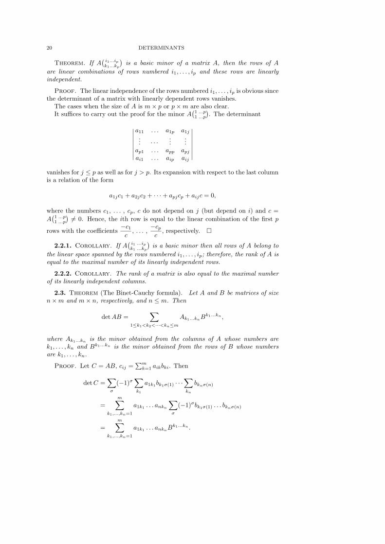
Theorem. If A(i1...ipk1...kp
)is a basic minor of a matrix A, then the rows of A
are linear combinations of rows numbered i1, . . . , ip and these rows are linearlyindependent.
Proof. The linear independence of the rows numbered i1, . . . , ip is obvious sincethe determinant of a matrix with linearly dependent rows vanishes.
The cases when the size of A is m× p or p×m are also clear.It suffices to carry out the proof for the minor A
(1 ...p1 ...p
). The determinant
∣∣∣∣∣∣∣∣
a11 . . . a1p a1j
... · · · ......
ap1 . . . app apjai1 . . . aip aij
∣∣∣∣∣∣∣∣
vanishes for j ≤ p as well as for j > p. Its expansion with respect to the last columnis a relation of the form
a1jc1 + a2jc2 + · · ·+ apjcp + aijc = 0,
where the numbers c1, . . . , cp, c do not depend on j (but depend on i) and c =A
(1 ...p1 ...p
) 6= 0. Hence, the ith row is equal to the linear combination of the first p
rows with the coefficients−c1c
, . . . ,−cpc
, respectively. ¤
2.2.1. Corollary. If A(i1 ...ipk1 ...kp
)is a basic minor then all rows of A belong to
the linear space spanned by the rows numbered i1, . . . , ip; therefore, the rank of A isequal to the maximal number of its linearly independent rows.
2.2.2. Corollary. The rank of a matrix is also equal to the maximal numberof its linearly independent columns.
2.3. Theorem (The Binet-Cauchy formula). Let A and B be matrices of sizen×m and m× n, respectively, and n ≤ m. Then
detAB =∑
1≤k1<k2<···<kn≤mAk1...knB
k1...kn ,
where Ak1...kn is the minor obtained from the columns of A whose numbers arek1, . . . , kn and Bk1...kn is the minor obtained from the rows of B whose numbersare k1, . . . , kn.
Proof. Let C = AB, cij =∑mk=1 aikbki. Then
detC =∑σ
(−1)σ∑
k1
a1k1bk1σ(1) · · ·∑
kn
bknσ(n)
=m∑
k1,...,kn=1
a1k1 . . . ankn∑σ
(−1)σbk1σ(1) . . . bknσ(n)
=m∑
k1,...,kn=1
a1k1 . . . anknBk1...kn .
2. MINORS AND COFACTORS 21
The minor Bk1...kn is nonzero only if the numbers k1, . . . , kn are distinct; there-fore, the summation can be performed over distinct numbers k1, . . . , kn. SinceBτ(k1)...τ(kn) = (−1)τBk1...kn for any permutation τ of the numbers k1, . . . , kn,then
m∑
k1,...,kn=1
a1k1 . . . anknBk1...kn =
∑
k1<k2<···<kn(−1)τa1τ(1) . . . anτ(n)B
k1...kn
=∑
1≤k1<k2<···<kn≤mAk1...knB
k1...kn . ¤
Remark. Another proof is given in the solution of Problem 28.7
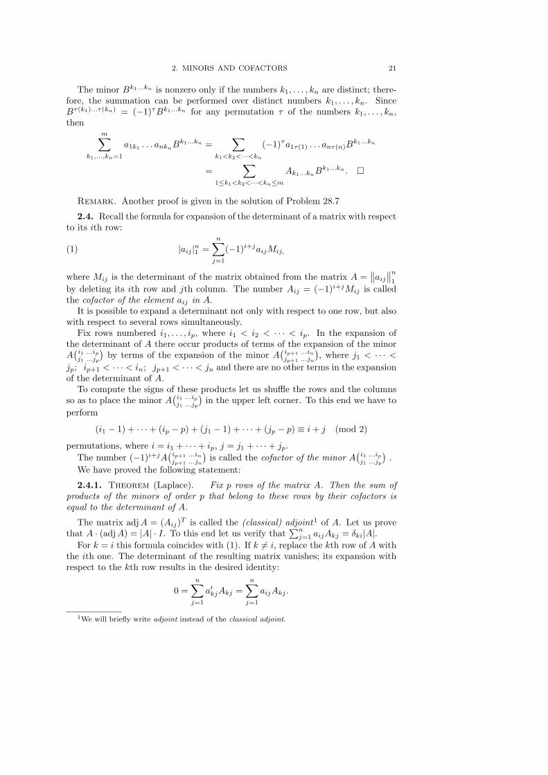
2.4. Recall the formula for expansion of the determinant of a matrix with respectto its ith row:
(1) |aij |n1 =n∑
j=1
(−1)i+jaijMij,
where Mij is the determinant of the matrix obtained from the matrix A =∥∥aij
∥∥n1
by deleting its ith row and jth column. The number Aij = (−1)i+jMij is calledthe cofactor of the element aij in A.
It is possible to expand a determinant not only with respect to one row, but alsowith respect to several rows simultaneously.
Fix rows numbered i1, . . . , ip, where i1 < i2 < · · · < ip. In the expansion ofthe determinant of A there occur products of terms of the expansion of the minorA
(i1 ...ipj1 ...jp
)by terms of the expansion of the minor A
(ip+1 ...injp+1 ...jn
), where j1 < · · · <
jp; ip+1 < · · · < in; jp+1 < · · · < jn and there are no other terms in the expansionof the determinant of A.
To compute the signs of these products let us shuffle the rows and the columnsso as to place the minor A
(i1 ...ipj1 ...jp
)in the upper left corner. To this end we have to
perform
(i1 − 1) + · · ·+ (ip − p) + (j1 − 1) + · · ·+ (jp − p) ≡ i+ j (mod 2)
permutations, where i = i1 + · · ·+ ip, j = j1 + · · ·+ jp.The number (−1)i+jA
(ip+1 ...injp+1 ...jn
)is called the cofactor of the minor A
(i1 ...ipj1 ...jp
).
We have proved the following statement:
2.4.1. Theorem (Laplace). Fix p rows of the matrix A. Then the sum ofproducts of the minors of order p that belong to these rows by their cofactors isequal to the determinant of A.
The matrix adjA = (Aij)T is called the (classical) adjoint1 of A. Let us provethat A · (adjA) = |A| · I. To this end let us verify that
∑nj=1 aijAkj = δki|A|.
For k = i this formula coincides with (1). If k 6= i, replace the kth row of A withthe ith one. The determinant of the resulting matrix vanishes; its expansion withrespect to the kth row results in the desired identity:
0 =n∑
j=1
a′kjAkj =n∑
j=1
aijAkj .
1We will briefly write adjoint instead of the classical adjoint.
22 DETERMINANTS
If A is invertible then A−1 =adjA|A| .
2.4.2. Theorem. The operation adj has the following properties:a) adjAB = adjB · adjA;b) adjXAX−1 = X(adjA)X−1;c) if AB = BA then (adjA)B = B(adjA).
Proof. If A and B are invertible matrices, then (AB)−1 = B−1A−1. Since foran invertible matrix A we have adjA = A−1|A|, headings a) and b) are obvious.Let us consider heading c).
If AB = BA and A is invertible, then
A−1B = A−1(BA)A−1 = A−1(AB)A−1 = BA−1.
Therefore, for invertible matrices the theorem is obvious.In each of the equations a) – c) both sides continuously depend on the elements of
A and B. Any matrix A can be approximated by matrices of the form Aε = A+ εIwhich are invertible for sufficiently small nonzero ε. (Actually, if a1, . . . , ar is thewhole set of eigenvalues of A, then Aε is invertible for all ε 6= −ai.) Besides, ifAB = BA, then AεB = BAε. ¤
2.5. The relations between the minors of a matrix A and the complementary tothem minors of the matrix (adjA)T are rather simple.
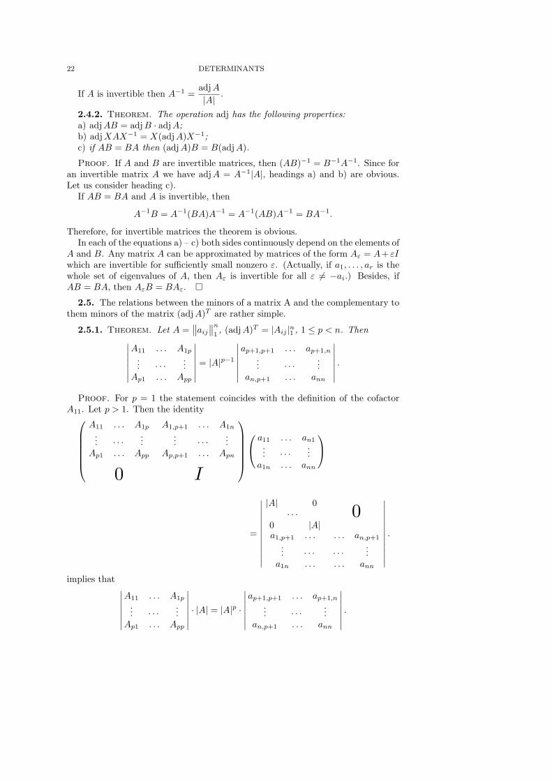
2.5.1. Theorem. Let A =∥∥aij
∥∥n1
, (adjA)T = |Aij |n1 , 1 ≤ p < n. Then∣∣∣∣∣∣∣
A11 . . . A1p
... · · · ...Ap1 . . . App
∣∣∣∣∣∣∣= |A|p−1
∣∣∣∣∣∣∣
ap+1,p+1 . . . ap+1,n
... · · · ...an,p+1 . . . ann
∣∣∣∣∣∣∣.
Proof. For p = 1 the statement coincides with the definition of the cofactorA11. Let p > 1. Then the identity
A11 . . . A1p
... · · · ...Ap1 . . . App
A1,p+1 . . . A1n
... · · · ...Ap,p+1 . . . Apn
0 I
a11 . . . an1... · · · ...a1n . . . ann
=
∣∣∣∣∣∣∣∣∣∣∣∣
|A| 0· · ·
0 |A|0
a1,p+1 . . .... · · ·a1n . . .
. . . an,p+1
· · · .... . . ann
∣∣∣∣∣∣∣∣∣∣∣∣
.
implies that∣∣∣∣∣∣∣
A11 . . . A1p
... · · · ...Ap1 . . . App
∣∣∣∣∣∣∣· |A| = |A|p ·
∣∣∣∣∣∣∣
ap+1,p+1 . . . ap+1,n
... · · · ...an,p+1 . . . ann
∣∣∣∣∣∣∣.
2. MINORS AND COFACTORS 23
If |A| 6= 0, then dividing by |A| we get the desired conclusion. For |A| = 0 thestatement follows from the continuity of the both parts of the desired identity withrespect to aij . ¤
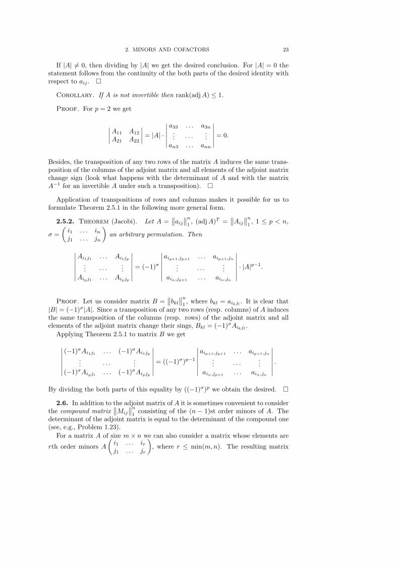
Corollary. If A is not invertible then rank(adjA) ≤ 1.
Proof. For p = 2 we get
∣∣∣∣A11 A12
A21 A22
∣∣∣∣ = |A| ·∣∣∣∣∣∣
a33 . . . a3n... · · · ...an3 . . . ann
∣∣∣∣∣∣= 0.
Besides, the transposition of any two rows of the matrix A induces the same trans-position of the columns of the adjoint matrix and all elements of the adjoint matrixchange sign (look what happens with the determinant of A and with the matrixA−1 for an invertible A under such a transposition). ¤
Application of transpositions of rows and columns makes it possible for us toformulate Theorem 2.5.1 in the following more general form.
2.5.2. Theorem (Jacobi). Let A =∥∥aij
∥∥n1
, (adjA)T =∥∥Aij
∥∥n1
, 1 ≤ p < n,
σ =(i1 . . . inj1 . . . jn
)an arbitrary permutation. Then
∣∣∣∣∣∣∣
Ai1j1 . . . Ai1jp... · · · ...
Aipj1 . . . Aipjp
∣∣∣∣∣∣∣= (−1)σ
∣∣∣∣∣∣∣
aip+1,jp+1 . . . aip+1,jn
... · · · ...ain,jp+1 . . . ain,jn
∣∣∣∣∣∣∣· |A|p−1.
Proof. Let us consider matrix B =∥∥bkl
∥∥n1, where bkl = aikjl . It is clear that
|B| = (−1)σ|A|. Since a transposition of any two rows (resp. columns) of A inducesthe same transposition of the columns (resp. rows) of the adjoint matrix and allelements of the adjoint matrix change their sings, Bkl = (−1)σAikjl .
Applying Theorem 2.5.1 to matrix B we get
∣∣∣∣∣∣∣
(−1)σAi1j1 . . . (−1)σAi1jp... · · · ...
(−1)σAipj1 . . . (−1)σAipjp
∣∣∣∣∣∣∣= ((−1)σ)p−1
∣∣∣∣∣∣∣
aip+1,jp+1 . . . aip+1,jn
... · · · ...ain,jp+1 . . . ain,jn
∣∣∣∣∣∣∣.
By dividing the both parts of this equality by ((−1)σ)p we obtain the desired. ¤
2.6. In addition to the adjoint matrix of A it is sometimes convenient to considerthe compound matrix
∥∥Mij
∥∥n1
consisting of the (n − 1)st order minors of A. Thedeterminant of the adjoint matrix is equal to the determinant of the compound one(see, e.g., Problem 1.23).
For a matrix A of size m× n we can also consider a matrix whose elements are
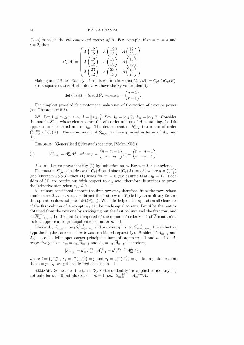
rth order minors A(i1 . . . irj1 . . . jr
), where r ≤ min(m,n). The resulting matrix
24 DETERMINANTS
Cr(A) is called the rth compound matrix of A. For example, if m = n = 3 andr = 2, then
C2(A) =
A
(1212
)A
(1213
)A
(1223
)
A
(1312
)A
(1313
)A
(1323
)
A
(2312
)A
(2313
)A
(2323
)
.
Making use of Binet–Cauchy’s formula we can show that Cr(AB) = Cr(A)Cr(B).For a square matrix A of order n we have the Sylvester identity
detCr(A) = (detA)p, where p =(n− 1r − 1
).
The simplest proof of this statement makes use of the notion of exterior power(see Theorem 28.5.3).
2.7. Let 1 ≤ m ≤ r < n, A =∥∥aij
∥∥n1. Set An = |aij |n1 , Am = |aij |m1 . Consider
the matrix Srm,n whose elements are the rth order minors of A containing the leftupper corner principal minor Am. The determinant of Srm,n is a minor of order(n−mr−m
)of Cr(A). The determinant of Srm,n can be expressed in terms of Am and
An.
Theorem (Generalized Sylvester’s identity, [Mohr,1953]).
(1) |Srm,n| = ApmAqn, where p =
(n−m− 1r −m
), q =
(n−m− 1r −m− 1
).
Proof. Let us prove identity (1) by induction on n. For n = 2 it is obvious.The matrix Sr0,n coincides with Cr(A) and since |Cr(A)| = Aqn, where q =
(n−1r−1
)(see Theorem 28.5.3), then (1) holds for m = 0 (we assume that A0 = 1). Bothsides of (1) are continuous with respect to aij and, therefore, it suffices to provethe inductive step when a11 6= 0.
All minors considered contain the first row and, therefore, from the rows whosenumbers are 2, . . . , n we can subtract the first row multiplied by an arbitrary factor;this operation does not affect det(Srm,n). With the help of this operation all elementsof the first column of A except a11 can be made equal to zero. Let A be the matrixobtained from the new one by strikinging out the first column and the first row, andlet S
r−1
m−1,n−1 be the matrix composed of the minors of order r − 1 of A containingits left upper corner principal minor of order m− 1.
Obviously, Srm,n = a11Sr−1
m−1,n−1 and we can apply to Sr−1
m−1,n−1 the inductivehypothesis (the case m − 1 = 0 was considered separately). Besides, if Am−1 andAn−1 are the left upper corner principal minors of orders m − 1 and n − 1 of A,respectively, then Am = a11Am−1 and An = a11An−1. Therefore,
|Srm,n| = at11Ap1
m−1Aq1n−1 = at−p1−q1
11 Ap1mA
q1n ,
where t =(n−mr−m
), p1 =
(n−m−1r−m
)= p and q1 =
(n−m−1r−m−1
)= q. Taking into account
that t = p+ q, we get the desired conclusion. ¤Remark. Sometimes the term “Sylvester’s identity” is applied to identity (1)
not only for m = 0 but also for r = m+ 1, i.e., |Sm+1m,n | = An−mm An
2. MINORS AND COFACTORS 25
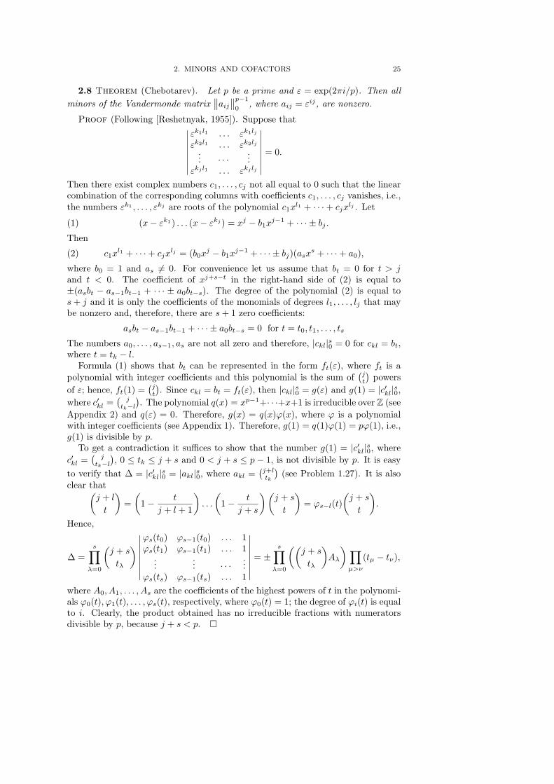
2.8 Theorem (Chebotarev). Let p be a prime and ε = exp(2πi/p). Then allminors of the Vandermonde matrix
∥∥aij∥∥p−1
0, where aij = εij, are nonzero.
Proof (Following [Reshetnyak, 1955]). Suppose that∣∣∣∣∣∣∣∣
εk1l1 . . . εk1lj
εk2l1 . . . εk2lj
... · · · ...εkj l1 . . . εkj lj
∣∣∣∣∣∣∣∣= 0.
Then there exist complex numbers c1, . . . , cj not all equal to 0 such that the linearcombination of the corresponding columns with coefficients c1, . . . , cj vanishes, i.e.,the numbers εk1 , . . . , εkj are roots of the polynomial c1xl1 + · · ·+ cjx
lj . Let
(1) (x− εk1) . . . (x− εkj ) = xj − b1xj−1 + · · · ± bj .Then
(2) c1xl1 + · · ·+ cjx
lj = (b0xj − b1xj−1 + · · · ± bj)(asxs + · · ·+ a0),
where b0 = 1 and as 6= 0. For convenience let us assume that bt = 0 for t > jand t < 0. The coefficient of xj+s−t in the right-hand side of (2) is equal to±(asbt − as−1bt−1 + · · · ± a0bt−s). The degree of the polynomial (2) is equal tos+ j and it is only the coefficients of the monomials of degrees l1, . . . , lj that maybe nonzero and, therefore, there are s+ 1 zero coefficients:
asbt − as−1bt−1 + · · · ± a0bt−s = 0 for t = t0, t1, . . . , ts
The numbers a0, . . . , as−1, as are not all zero and therefore, |ckl|s0 = 0 for ckl = bt,where t = tk − l.
Formula (1) shows that bt can be represented in the form ft(ε), where ft is apolynomial with integer coefficients and this polynomial is the sum of
(jt
)powers
of ε; hence, ft(1) =(jt
). Since ckl = bt = ft(ε), then |ckl|s0 = g(ε) and g(1) = |c′kl|s0,
where c′kl =(
jtk−l
). The polynomial q(x) = xp−1+· · ·+x+1 is irreducible over Z (see
Appendix 2) and q(ε) = 0. Therefore, g(x) = q(x)ϕ(x), where ϕ is a polynomialwith integer coefficients (see Appendix 1). Therefore, g(1) = q(1)ϕ(1) = pϕ(1), i.e.,g(1) is divisible by p.
To get a contradiction it suffices to show that the number g(1) = |c′kl|s0, wherec′kl =
(j
tk−l), 0 ≤ tk ≤ j + s and 0 < j + s ≤ p− 1, is not divisible by p. It is easy
to verify that ∆ = |c′kl|s0 = |akl|s0, where akl =(j+ltk
)(see Problem 1.27). It is also
clear that(j + l
t
)=
(1− t
j + l + 1
). . .
(1− t
j + s
)(j + s
t
)= ϕs−l(t)
(j + s
t
).
Hence,
∆ =s∏
λ=0
(j + s
tλ
)∣∣∣∣∣∣∣∣
ϕs(t0) ϕs−1(t0) . . . 1ϕs(t1) ϕs−1(t1) . . . 1
...... · · · ...
ϕs(ts) ϕs−1(ts) . . . 1
∣∣∣∣∣∣∣∣= ±
s∏
λ=0
((j + s
tλ
)Aλ
) ∏µ>ν
(tµ − tν),
where A0, A1, . . . , As are the coefficients of the highest powers of t in the polynomi-als ϕ0(t), ϕ1(t), . . . , ϕs(t), respectively, where ϕ0(t) = 1; the degree of ϕi(t) is equalto i. Clearly, the product obtained has no irreducible fractions with numeratorsdivisible by p, because j + s < p. ¤
26 DETERMINANTS
Problems
2.1. Let An be a matrix of size n×n. Prove that |A+λI| = λn+∑nk=1 Skλ
n−k,where Sk is the sum of all
(nk
)principal kth order minors of A.
2.2. Prove that∣∣∣∣∣∣∣∣
a11 . . . a1n x1... · · · ...
...an1 . . . ann xny1 . . . yn 0
∣∣∣∣∣∣∣∣= −
∑
i,j
xiyjAij ,
where Aij is the cofactor of aij in∥∥aij
∥∥n1.
2.3. Prove that the sum of principal k-minors of ATA is equal to the sum ofsquares of all k-minors of A.
2.4. Prove that∣∣∣∣∣∣∣∣
u1a11 . . . una1n
a21 . . . a2n... · · · ...an1 . . . ann
∣∣∣∣∣∣∣∣+ · · ·+
∣∣∣∣∣∣∣∣
a11 . . . a1n
a21 . . . a2n... · · · ...
u1an1 . . . unann
∣∣∣∣∣∣∣∣= (u1 + · · ·+ un)|A|.
Inverse and adjoint matrices
2.5. Let A and B be square matrices of order n. ComputeI A C0 I B0 0 I
−1
.
2.6. Prove that the matrix inverse to an invertible upper triangular matrix isalso an upper triangular one.
2.7. Give an example of a matrix of order n whose adjoint has only one nonzeroelement and this element is situated in the ith row and jth column for given i andj.
2.8. Let x and y be columns of length n. Prove that
adj(I − xyT ) = xyT + (1− yTx)I.
2.9. Let A be a skew-symmetric matrix of order n. Prove that adjA is a sym-metric matrix for odd n and a skew-symmetric one for even n.
2.10. Let An be a skew-symmetric matrix of order n with elements +1 abovethe main diagonal. Calculate adjAn.
2.11. The matrix adj(A− λI) can be expressed in the form∑n−1k=0 λ
kAk, wheren is the order of A. Prove that:
a) for any k (1 ≤ k ≤ n− 1) the matrix AkA−Ak−1 is a scalar matrix;b) the matrix An−s can be expressed as a polynomial of degree s− 1 in A.2.12. Find all matrices A with nonnegative elements such that all elements of
A−1 are also nonnegative.2.13. Let ε = exp(2πi/n); A =
∥∥aij∥∥n
1, where aij = εij . Calculate the matrix
A−1.2.14. Calculate the matrix inverse to the Vandermonde matrix V .
3. THE SCHUR COMPLEMENT 27
3. The Schur complement
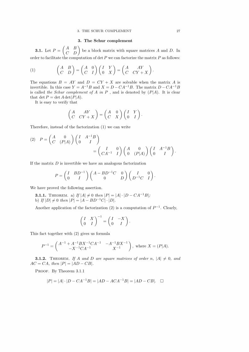
3.1. Let P =(A BC D
)be a block matrix with square matrices A and D. In
order to facilitate the computation of detP we can factorize the matrix P as follows:
(1)(A BC D
)=
(A 0C I
)(I Y0 X
)=
(A AYC CY +X
).
The equations B = AY and D = CY + X are solvable when the matrix A isinvertible. In this case Y = A−1B and X = D−CA−1B. The matrix D−CA−1Bis called the Schur complement of A in P , and is denoted by (P |A). It is clearthat detP = detAdet(P |A).
It is easy to verify that
(A AYC CY +X
)=
(A 0C X
)(I Y0 I
).
Therefore, instead of the factorization (1) we can write
(2) P =(A 0C (P |A)
)(I A−1B0 I
)
=(
I 0CA−1 I
) (A 00 (P |A)
)(I A−1B0 I
).
If the matrix D is invertible we have an analogous factorization
P =(I BD−1
0 I
)(A−BD−1C 0
0 D
)(I 0
D−1C I
).
We have proved the following assertion.
3.1.1. Theorem. a) If |A| 6= 0 then |P | = |A| · |D − CA−1B|;b) If |D| 6= 0 then |P | = |A−BD−1C| · |D|.Another application of the factorization (2) is a computation of P−1. Clearly,
(I X0 I
)−1
=(I −X0 I
).
This fact together with (2) gives us formula
P−1 =(A−1 +A−1BX−1CA−1 −A−1BX−1
−X−1CA−1 X−1
), where X = (P |A).
3.1.2. Theorem. If A and D are square matrices of order n, |A| 6= 0, andAC = CA, then |P | = |AD − CB|.
Proof. By Theorem 3.1.1
|P | = |A| · |D − CA−1B| = |AD −ACA−1B| = |AD − CB|. ¤
28 DETERMINANTS
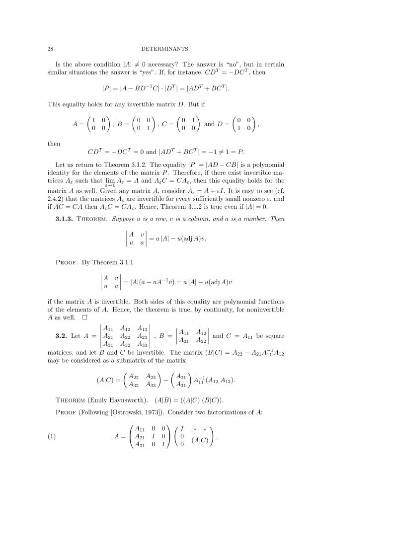
Is the above condition |A| 6= 0 necessary? The answer is “no”, but in certainsimilar situations the answer is “yes”. If, for instance, CDT = −DCT , then
|P | = |A−BD−1C| · |DT | = |ADT +BCT |.
This equality holds for any invertible matrix D. But if
A =(
1 00 0
), B =
(0 00 1
), C =
(0 10 0
)and D =
(0 01 0
),
thenCDT = −DCT = 0 and |ADT +BCT | = −1 6= 1 = P.
Let us return to Theorem 3.1.2. The equality |P | = |AD −CB| is a polynomialidentity for the elements of the matrix P . Therefore, if there exist invertible ma-trices Aε such that lim
ε→0Aε = A and AεC = CAε, then this equality holds for the
matrix A as well. Given any matrix A, consider Aε = A+ εI. It is easy to see (cf.2.4.2) that the matrices Aε are invertible for every sufficiently small nonzero ε, andif AC = CA then AεC = CAε. Hence, Theorem 3.1.2 is true even if |A| = 0.
3.1.3. Theorem. Suppose u is a row, v is a column, and a is a number. Then
∣∣∣∣A vu a
∣∣∣∣ = a |A| − u(adjA)v.
Proof. By Theorem 3.1.1
∣∣∣∣A vu a
∣∣∣∣ = |A|(a− uA−1v) = a |A| − u(adjA)v
if the matrix A is invertible. Both sides of this equality are polynomial functionsof the elements of A. Hence, the theorem is true, by continuity, for noninvertibleA as well. ¤
3.2. Let A =
∣∣∣∣∣∣
A11 A12 A13
A21 A22 A23
A31 A32 A33
∣∣∣∣∣∣, B =
∣∣∣∣A11 A12
A21 A22
∣∣∣∣ and C = A11 be square
matrices, and let B and C be invertible. The matrix (B|C) = A22 − A21A−111 A12
may be considered as a submatrix of the matrix
(A|C) =(A22 A23
A32 A33
)−
(A21
A31
)A−1
11 (A12 A13).
Theorem (Emily Haynsworth). (A|B) = ((A|C)|(B|C)).
Proof (Following [Ostrowski, 1973]). Consider two factorizations of A:
(1) A =
A11 0 0A21 I 0A31 0 I
(I ∗ ∗00 (A|C)
),
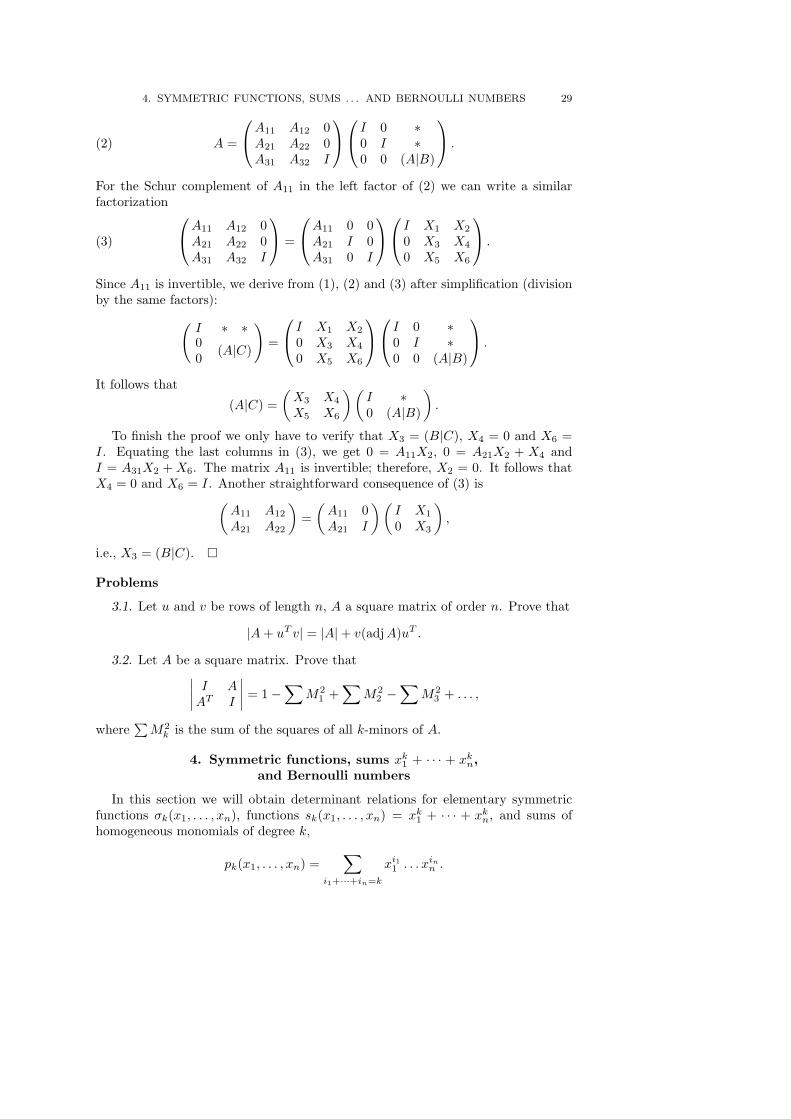
4. SYMMETRIC FUNCTIONS, SUMS . . . AND BERNOULLI NUMBERS 29
(2) A =
A11 A12 0A21 A22 0A31 A32 I
I 0 ∗0 I ∗0 0 (A|B)
.
For the Schur complement of A11 in the left factor of (2) we can write a similarfactorization
(3)
A11 A12 0A21 A22 0A31 A32 I
=
A11 0 0A21 I 0A31 0 I
I X1 X2
0 X3 X4
0 X5 X6
.
Since A11 is invertible, we derive from (1), (2) and (3) after simplification (divisionby the same factors):
(I ∗ ∗00 (A|C)
)=
I X1 X2
0 X3 X4
0 X5 X6
I 0 ∗0 I ∗0 0 (A|B)
.
It follows that
(A|C) =(X3 X4
X5 X6
)(I ∗0 (A|B)
).
To finish the proof we only have to verify that X3 = (B|C), X4 = 0 and X6 =I. Equating the last columns in (3), we get 0 = A11X2, 0 = A21X2 + X4 andI = A31X2 + X6. The matrix A11 is invertible; therefore, X2 = 0. It follows thatX4 = 0 and X6 = I. Another straightforward consequence of (3) is
(A11 A12
A21 A22
)=
(A11 0A21 I
)(I X1
0 X3
),
i.e., X3 = (B|C). ¤
Problems
3.1. Let u and v be rows of length n, A a square matrix of order n. Prove that
|A+ uT v| = |A|+ v(adjA)uT .
3.2. Let A be a square matrix. Prove that∣∣∣∣I AAT I
∣∣∣∣ = 1−∑
M21 +
∑M2
2 −∑
M23 + . . . ,
where∑M2k is the sum of the squares of all k-minors of A.
4. Symmetric functions, sums xk1 + · · · + xkn,and Bernoulli numbers
In this section we will obtain determinant relations for elementary symmetricfunctions σk(x1, . . . , xn), functions sk(x1, . . . , xn) = xk1 + · · · + xkn, and sums ofhomogeneous monomials of degree k,
pk(x1, . . . , xn) =∑
i1+···+in=k
xi11 . . . xinn .
30 DETERMINANTS
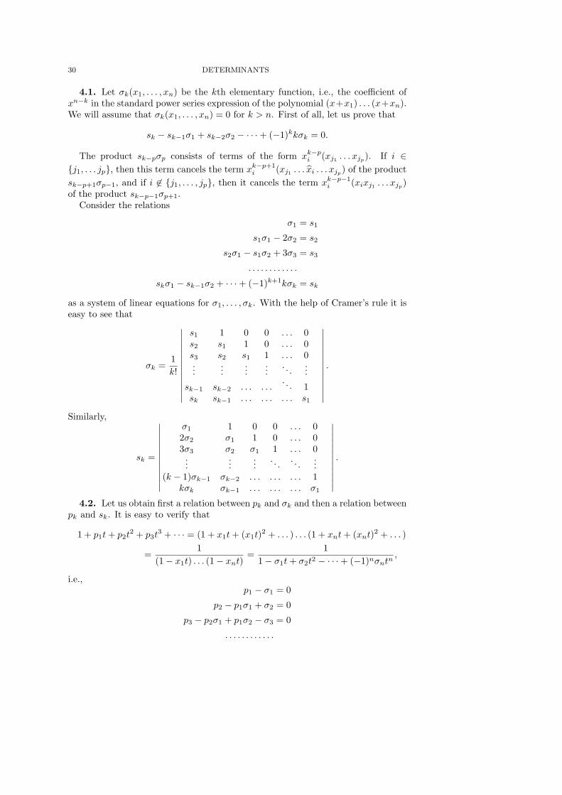
4.1. Let σk(x1, . . . , xn) be the kth elementary function, i.e., the coefficient ofxn−k in the standard power series expression of the polynomial (x+x1) . . . (x+xn).We will assume that σk(x1, . . . , xn) = 0 for k > n. First of all, let us prove that
sk − sk−1σ1 + sk−2σ2 − · · ·+ (−1)kkσk = 0.
The product sk−pσp consists of terms of the form xk−pi (xj1 . . . xjp). If i ∈j1, . . . jp, then this term cancels the term xk−p+1
i (xj1 . . . xi . . . xjp) of the productsk−p+1σp−1, and if i 6∈ j1, . . . , jp, then it cancels the term xk−p−1
i (xixj1 . . . xjp)of the product sk−p−1σp+1.
Consider the relations
σ1 = s1
s1σ1 − 2σ2 = s2
s2σ1 − s1σ2 + 3σ3 = s3
. . . . . . . . . . . .
skσ1 − sk−1σ2 + · · ·+ (−1)k+1kσk = sk
as a system of linear equations for σ1, . . . , σk. With the help of Cramer’s rule it iseasy to see that
σk =1k!
∣∣∣∣∣∣∣∣∣∣∣∣∣
s1 1 0 0 . . . 0s2 s1 1 0 . . . 0s3 s2 s1 1 . . . 0...
......
.... . .
...
sk−1 sk−2 . . . . . .. . . 1
sk sk−1 . . . . . . . . . s1
∣∣∣∣∣∣∣∣∣∣∣∣∣
.
Similarly,
sk =
∣∣∣∣∣∣∣∣∣∣∣∣
σ1 1 0 0 . . . 02σ2 σ1 1 0 . . . 03σ3 σ2 σ1 1 . . . 0
......
.... . . . . .
...(k − 1)σk−1 σk−2 . . . . . . . . . 1
kσk σk−1 . . . . . . . . . σ1
∣∣∣∣∣∣∣∣∣∣∣∣
.
4.2. Let us obtain first a relation between pk and σk and then a relation betweenpk and sk. It is easy to verify that
1 + p1t+ p2t2 + p3t
3 + · · · = (1 + x1t+ (x1t)2 + . . . ) . . . (1 + xnt+ (xnt)2 + . . . )
=1
(1− x1t) . . . (1− xnt) =1
1− σ1t+ σ2t2 − · · ·+ (−1)nσntn,
i.e.,p1 − σ1 = 0
p2 − p1σ1 + σ2 = 0
p3 − p2σ1 + p1σ2 − σ3 = 0
. . . . . . . . . . . .
4. SYMMETRIC FUNCTIONS, SUMS . . . AND BERNOULLI NUMBERS 31
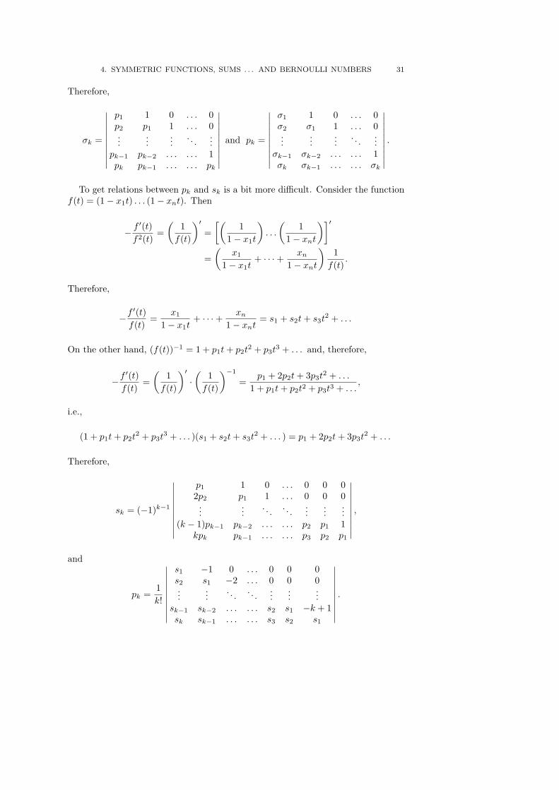
Therefore,
σk =
∣∣∣∣∣∣∣∣∣∣
p1 1 0 . . . 0p2 p1 1 . . . 0...
......
. . ....
pk−1 pk−2 . . . . . . 1pk pk−1 . . . . . . pk
∣∣∣∣∣∣∣∣∣∣
and pk =
∣∣∣∣∣∣∣∣∣∣
σ1 1 0 . . . 0σ2 σ1 1 . . . 0...
......
. . ....
σk−1 σk−2 . . . . . . 1σk σk−1 . . . . . . σk
∣∣∣∣∣∣∣∣∣∣
.
To get relations between pk and sk is a bit more difficult. Consider the functionf(t) = (1− x1t) . . . (1− xnt). Then
− f′(t)
f2(t)=
(1f(t)
)′=
[(1
1− x1t
). . .
(1
1− xnt)]′
=(
x1
1− x1t+ · · ·+ xn
1− xnt)
1f(t)
.
Therefore,
−f′(t)f(t)
=x1
1− x1t+ · · ·+ xn
1− xnt = s1 + s2t+ s3t2 + . . .
On the other hand, (f(t))−1 = 1 + p1t+ p2t2 + p3t
3 + . . . and, therefore,
−f′(t)f(t)
=(
1f(t)
)′·(
1f(t)
)−1
=p1 + 2p2t+ 3p3t
2 + . . .
1 + p1t+ p2t2 + p3t3 + . . .,
i.e.,
(1 + p1t+ p2t2 + p3t
3 + . . . )(s1 + s2t+ s3t2 + . . . ) = p1 + 2p2t+ 3p3t
2 + . . .
Therefore,
sk = (−1)k−1
∣∣∣∣∣∣∣∣∣∣
p1 1 0 . . . 0 0 02p2 p1 1 . . . 0 0 0
......
. . . . . ....
......
(k − 1)pk−1 pk−2 . . . . . . p2 p1 1kpk pk−1 . . . . . . p3 p2 p1
∣∣∣∣∣∣∣∣∣∣
,
and
pk =1k!
∣∣∣∣∣∣∣∣∣∣
s1 −1 0 . . . 0 0 0s2 s1 −2 . . . 0 0 0...
.... . . . . .
......
...sk−1 sk−2 . . . . . . s2 s1 −k + 1sk sk−1 . . . . . . s3 s2 s1
∣∣∣∣∣∣∣∣∣∣
.
32 DETERMINANTS
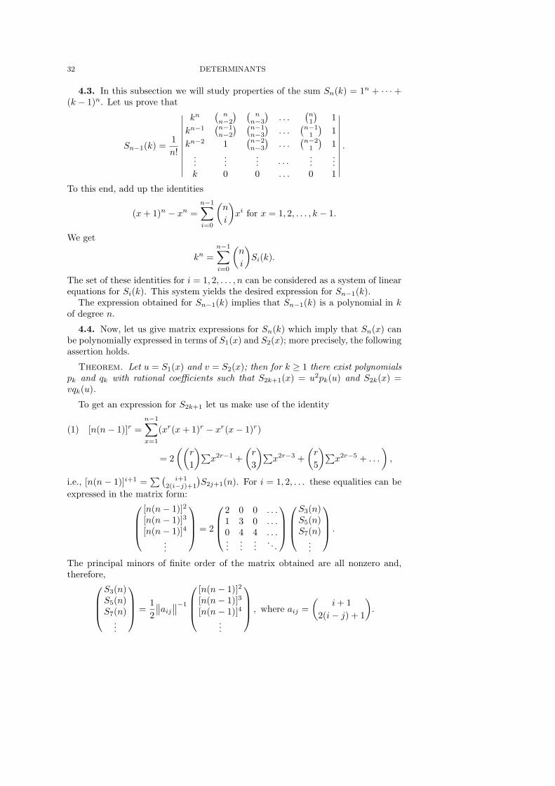
4.3. In this subsection we will study properties of the sum Sn(k) = 1n + · · · +(k − 1)n. Let us prove that
Sn−1(k) =1n!
∣∣∣∣∣∣∣∣∣∣∣
kn(nn−2
) (nn−3
). . .
(n1
)1
kn−1(n−1n−2
) (n−1n−3
). . .
(n−1
1
)1
kn−2 1(n−2n−3
). . .
(n−2
1
)1
......
... · · · ......
k 0 0 . . . 0 1
∣∣∣∣∣∣∣∣∣∣∣
.
To this end, add up the identities
(x+ 1)n − xn =n−1∑
i=0
(n
i
)xi for x = 1, 2, . . . , k − 1.
We get
kn =n−1∑
i=0
(n
i
)Si(k).
The set of these identities for i = 1, 2, . . . , n can be considered as a system of linearequations for Si(k). This system yields the desired expression for Sn−1(k).
The expression obtained for Sn−1(k) implies that Sn−1(k) is a polynomial in kof degree n.
4.4. Now, let us give matrix expressions for Sn(k) which imply that Sn(x) canbe polynomially expressed in terms of S1(x) and S2(x); more precisely, the followingassertion holds.
Theorem. Let u = S1(x) and v = S2(x); then for k ≥ 1 there exist polynomialspk and qk with rational coefficients such that S2k+1(x) = u2pk(u) and S2k(x) =vqk(u).
To get an expression for S2k+1 let us make use of the identity
(1) [n(n− 1)]r =n−1∑x=1
(xr(x+ 1)r − xr(x− 1)r)
= 2((
r
1
)∑x2r−1 +
(r
3
)∑x2r−3 +
(r
5
)∑x2r−5 + . . .
),
i.e., [n(n − 1)]i+1 =∑(
i+12(i−j)+1
)S2j+1(n). For i = 1, 2, . . . these equalities can be
expressed in the matrix form:
[n(n− 1)]2
[n(n− 1)]3
[n(n− 1)]4...
= 2
2 0 0 . . .1 3 0 . . .0 4 4 . . ....
......
. . .
S3(n)S5(n)S7(n)
...
.
The principal minors of finite order of the matrix obtained are all nonzero and,therefore,
S3(n)S5(n)S7(n)
...
=
12
∥∥aij∥∥−1
[n(n− 1)]2
[n(n− 1)]3
[n(n− 1)]4...
, where aij =
(i+ 1
2(i− j) + 1
).
4. SYMMETRIC FUNCTIONS, SUMS . . . AND BERNOULLI NUMBERS 33
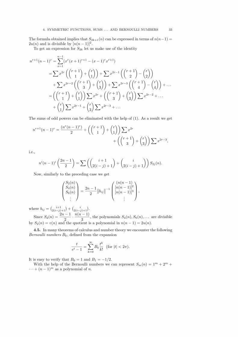
The formula obtained implies that S2k+1(n) can be expressed in terms of n(n−1) =2u(n) and is divisible by [n(n− 1)]2.
To get an expression for S2k let us make use of the identity
nr+1(n− 1)r =n−1∑x=1
(xr(x+ 1)r+1 − (x− 1)rxr+1)
=∑
x2r
((r + 1
1
)+
(r
1
))+
∑x2r−1
((r + 1
2
)−
(r
2
))
+∑
x2r−2
((r + 1
3
)+
(r
3
))+
∑x2r−3
((r + 1
4
)−
(r
4
))+ . . .
=((
r + 11
)+
(r
1
))∑x2r +
((r + 1
3
)+
(r
3
))∑x2r−2 + . . .
+(r
1
) ∑x2r−1 +
(r
3
) ∑x2r−3 + . . .
The sums of odd powers can be eliminated with the help of (1). As a result we get
nr+1(n− 1)r =(nr(n− 1)r)
2+
((r + 1
1
)+
(r
1
))∑x2r
+((
r + 13
)+
(r
3
))∑x2r−3,
i.e.,
ni(n− 1)i(
2n− 12
)=
∑ ((i+ 1
2(i− j) + 1
)+
(i
2(i− j) + 1
))S2j(n).
Now, similarly to the preceding case we get
S2(n)S4(n)S6(n)
...
=
2n− 12
∥∥bij∥∥−1
(n(n− 1)[n(n− 1)]2
[n(n− 1)]3...
,
where bij =(
i+12(i−j)+1
)+
(i
2(i−j)+1
).
Since S2(n) =2n− 1
2· n(n− 1)
3, the polynomials S4(n), S6(n), . . . are divisible
by S2(n) = v(n) and the quotient is a polynomial in n(n− 1) = 2u(n).
4.5. In many theorems of calculus and number theory we encounter the followingBernoulli numbers Bk, defined from the expansion
t
et − 1=∞∑
k=0
Bktk
k!(for |t| < 2π).
It is easy to verify that B0 = 1 and B1 = −1/2.With the help of the Bernoulli numbers we can represent Sm(n) = 1m + 2m +
· · ·+ (n− 1)m as a polynomial of n.
34 DETERMINANTS
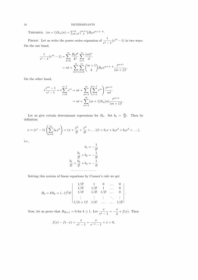
Theorem. (m+ 1)Sm(n) =∑mk=0
(m+1k
)Bkn
m+1−k.
Proof. Let us write the power series expansion oft
et − 1(ent − 1) in two ways.
On the one hand,
t
et − 1(ent − 1) =
∞∑
k=0
Bktk
k!
∞∑s=1
(nt)s
s!
= nt+∞∑m=1
m∑
k=0
(m+ 1k
)Bkn
m+1−k tm+1
(m+ 1)!.
On the other hand,
tent − 1et − 1
= t
n−1∑r=0
ert = nt+∞∑m=1
(n−1∑r=1
rm
)tm+1
m!
= nt+∞∑m=1
(m+ 1)Sm(n)tm+1
(m+ 1)!.
Let us give certain determinant expressions for Bk. Set bk = Bkk! . Then by
definition
x = (ex − 1)
( ∞∑
k=0
bkxk
)= (x+
x2
2!+x3
3!+ . . . )(1 + b1x+ b2x
2 + b3x3 + . . . ),
i.e.,
b1 = − 12!
b12!
+ b2 = − 13!
b13!
+b22!
+ b3 = − 14!
. . . . . . . . . . . . . . . . . .
Solving this system of linear equations by Cramer’s rule we get
Bk = k!bk = (−1)kk!
∣∣∣∣∣∣∣∣∣∣
1/2! 1 0 . . . 01/3! 1/2! 1 . . . 01/4! 1/3! 1/2! . . . 0
......
.... . .
...1/(k + 1)! 1/k! . . . . . . 1/2!
∣∣∣∣∣∣∣∣∣∣
.
Now, let us prove that B2k+1 = 0 for k ≥ 1. Letx
ex − 1= −x
2+ f(x). Then
f(x)− f(−x) =x
ex − 1+
x
e−x − 1+ x = 0,
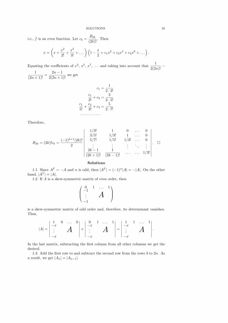
SOLUTIONS 35
i.e., f is an even function. Let ck =B2k
(2k)!. Then
x =(x+
x2
2!+x3
3!+ . . .
) (1− x
2+ c1x
2 + c2x4 + c3x
6 + . . .).
Equating the coefficients of x3, x5, x7, . . . and taking into account that1
2(2n)!−
1(2n+ 1)!
=2n− 1
2(2n+ 1)!we get
c1 =1
2 · 3!c13!
+ c2 =3
2 · 5!c15!
+c23!
+ c3 =5
2 · 7!. . . . . . . . . . . .
Therefore,
B2k = (2k)!ck =(−1)k+1(2k)!
2
∣∣∣∣∣∣∣∣∣∣∣∣
1/3! 1 0 . . . 03/5! 1/3! 1 . . . 05/7! 1/5! 1/3! . . . 0
......
.... . .
...2k − 1
(2k + 1)!1
(2k − 1)!. . . . . . 1/3!
∣∣∣∣∣∣∣∣∣∣∣∣
. ¤
Solutions
1.1. Since AT = −A and n is odd, then |AT | = (−1)n|A| = −|A|. On the otherhand, |AT | = |A|.
1.2. If A is a skew-symmetric matrix of even order, then
0 1 . . . 1−1...−1
A
is a skew-symmetric matrix of odd order and, therefore, its determinant vanishes.Thus,
|A| =
∣∣∣∣∣∣∣
1 0 . . . 0−x...−x
A
∣∣∣∣∣∣∣+
∣∣∣∣∣∣∣
0 1 . . . 1−x...−x
A
∣∣∣∣∣∣∣=
∣∣∣∣∣∣∣
1 1 . . . 1−x...−x
A
∣∣∣∣∣∣∣.
In the last matrix, subtracting the first column from all other columns we get thedesired.
1.3. Add the first row to and subtract the second row from the rows 3 to 2n. Asa result, we get |An| = |An−1|.
36 DETERMINANTS
1.4. Suppose that all terms of the expansion of an nth order determinant arepositive. If the intersection of two rows and two columns of the determinant singles
out a matrix(x yu v
)then the expansion of the determinant has terms of the
form xvα and −yuα and, therefore, sign(xv) = − sign(yu). Let ai, bi and ci bethe first three elements of the ith row (i = 1, 2). Then sign(a1b2) = − sign(a2b1),sign(b1c2) = − sign(b2c1), and sign(c1a2) = − sign(c2a1). By multiplying theseidentities we get sign p = − sign p, where p = a1b1c1a2b2c2. Contradiction.
1.5. For all i ≥ 2 let us subtract the (i − 1)st row multiplied by a from the ithrow. As a result we get an upper triangular matrix with diagonal elements a11 = 1and aii = 1− a2 for i > 1. The determinant of this matrix is equal to (1− a2)n−1.
1.6. Expanding the determinant ∆n+1 with respect to the last column we get
∆n+1 = x∆n + h∆n = (x+ h)∆n.
1.7. Let us prove that the desired determinant is equal to
∏(xi − aibi)
(1 +
∑
i
aibixi − aibi
)
by induction on n. For n = 2 this statement is easy to verify. We will carry outthe proof of the inductive step for n = 3 (in the general case the proof is similar):
∣∣∣∣∣∣
x1 a1b2 a1b3a2b1 x2 a2b3a3b1 a3b2 x3
∣∣∣∣∣∣=
∣∣∣∣∣∣
x1 − a1b1 a1b2 a1b30 x2 a2b30 a3b2 x3
∣∣∣∣∣∣+
∣∣∣∣∣∣
a1b1 a1b2 a1b3a2b1 x2 a2b3a3b1 a3b2 x3
∣∣∣∣∣∣.
The first determinant is computed by inductive hypothesis and to compute thesecond one we have to break out from the first row the factor a1 and for all i ≥ 2subtract from the ith row the first row multiplied by ai.
1.8. It is easy to verify that det(I − A) = 1− c. The matrix A is the matrix ofthe transformation Aei = ci−1ei−1 and therefore, An = c1 . . . cnI. Hence,
(I +A+ · · ·+An−1)(I −A) = I −An = (1− c)I
and, therefore,(1− c) det(I +A+ · · ·+An−1) = (1− c)n.
For c 6= 1 by dividing by 1− c we get the required. The determinant of the matrixconsidered depends continuously on c1, . . . , cn and, therefore, the identity holds forc = 1 as well.
1.9. Since (1 − xiyj)−1 = (y−1j − xi)−1y−1
j , we have |aij |n1 = σ|bij |n1 , whereσ = (y1 . . . yn)−1 and bij = (y−1
j − xi)−1, i.e., |bij |n1 is a Cauchy determinant(see 1.3). Therefore,
|bij |n1 = σ−1∏
i>j
(yj − yi)(xj − xi)∏
i,j
(1− xiyj)−1.
1.10. For a fixed m consider the matrices An =∥∥aij
∥∥m0
, aij =(n+ij
). The matrix
A0 is a triangular matrix with diagonal (1, . . . , 1). Therefore, |A0| = 1. Besides,
SOLUTIONS 37
An+1 = AnB, where bi,i+1 = 1 (for i ≤ m − 1), bi,i = 1 and all other elements bijare zero.
1.11. Clearly, points A, B, . . . , F with coordinates (a2, a), . . . , (f2, f), respec-tively, lie on a parabola. By Pascal’s theorem the intersection points of the pairs ofstraight lines AB and DE, BC and EF , CD and FA lie on one straight line. It isnot difficult to verify that the coordinates of the intersection point of AB and DEare (
(a+ b)de− (d+ e)abd+ e− a− b ,
de− abd+ e− a− b
).
It remains to note that if points (x1, y1), (x2, y2) and (x3, y3) belong to one straightline then ∣∣∣∣∣∣
x1 y1 1x2 y2 1x3 y3 1
∣∣∣∣∣∣= 0.
Remark. Recall that Pascal’s theorem states that the opposite sides of a hexagoninscribed in a 2nd order curve intersect at three points that lie on one line. Its proofcan be found in books [Berger, 1977] and [Reid, 1988].
1.12. Let s = x1 + · · · + xn. Then the kth element of the last column is of theform
(s− xk)n−1 = (−xk)n−1 +n−2∑
i=0
pixik.
Therefore, adding to the last column a linear combination of the remaining columnswith coefficients −p0, . . . , −pn−2, respectively, we obtain the determinant
∣∣∣∣∣∣∣
1 x1 . . . xn−21 (−x1)n−1
...... · · · ...
...1 xn . . . xn−2
n (−xn)n−1
∣∣∣∣∣∣∣= (−1)n−1V (x1, . . . , xn).
1.13. Let ∆ be the required determinant. Multiplying the first row of thecorresponding matrix by x1, . . . , and the nth row by xn we get
σ∆ =
∣∣∣∣∣∣∣
x1 x21 . . . xn−1
1 σ...
... · · · ......
xn x2n . . . xn−1
n σ
∣∣∣∣∣∣∣, where σ = x1 . . . xn.
Therefore, ∆ = (−1)n−1V (x1, . . . , xn).1.14. Since
λn−ki (1 + λ2i )k = λni (λ−1
i + λi)k,
then|aij |n0 = (λ0 . . . λn)nV (µ0, . . . , µn), where µi = λ−1
i + λi.
1.15. Augment the matrix V with an (n + 1)st column consisting of the nthpowers and then add an extra first row (1,−x, x2, . . . , (−x)n). The resulting matrixW is also a Vandermonde matrix and, therefore,
detW = (x+ x1) . . . (x+ xn) detV = (σn + σn−1x+ · · ·+ xn) detV.
38 DETERMINANTS
On the other hand, expanding W with respect to the first row we get
detW = detV0 + xdetV1 + · · ·+ xn detVn−1.
1.16. Let xi = in. Then
ai1 = xi, ai2 =xi(xi − 1)
2, . . . , air =
xi(xi − 1) . . . (xi − r + 1)r!
,
i.e., in the kth column there stand identical polynomials of kth degree in xi. Sincethe determinant does not vary if to one of its columns we add a linear combinationof its other columns, the determinant can be reduced to the form |bik|r1, where
bik =xkik!
=nk
k!ik. Therefore,
|aik|r1 = |bik|r1 = n · n2
2!. . .
nr
r!r!V (1, 2, . . . , r) = nr(r+1)/2,
because∏
1≤j<i≤r(i− j) = 2!3! . . . (r − 1)!1.17. For i = 1, . . . , n let us multiply the ith row of the matrix
∥∥aij∥∥n
1by mi!,
where mi = ki + n− i. We obtain the determinant |bij |n1 , where
bij =(ki + n− i)!(ki + j − i)! = mi(mi − 1) . . . (mi + j + 1− n).
The elements of the jth row of∥∥bij
∥∥n1
are identical polynomials of degree n − jin mi and the coefficients of the highest terms of these polynomials are equalto 1. Therefore, subtracting from every column linear combinations of the pre-ceding columns we can reduce the determinant |bij |n1 to a determinant with rows(mn−1
i ,mn−2i , . . . , 1). This determinant is equal to
∏i<j(mi −mj). It is also clear
that |aij |n1 = |bij |n1 (m1!m2! . . .mn!)−1.1.18. For n = 3 it is easy to verify that
∥∥aij∥∥2
0=
1 1 1x1 x2 x3
x21 x2
2 x23
p1 p1x1 p1x
21
p2 p2x2 p2x22
p3 p3x3 p3x23
.
In the general case an analogous identity holds.1.19. The required determinant can be represented in the form of a product of
two determinants:
∣∣∣∣∣∣∣∣∣∣
1 . . . 1 1x1 . . . xn yx2
1 . . . x2n y2
... · · · ......
xn1 . . . xnn yn
∣∣∣∣∣∣∣∣∣∣
·
∣∣∣∣∣∣∣∣∣∣∣
1 x1 . . . xn−11 0
1 x2 . . . xn−12 0
...... · · · ...
...1 xn . . . xn−1
n 00 0 . . . 0 1
∣∣∣∣∣∣∣∣∣∣∣
and, therefore, it is equal to∏
(y − xi)∏i>j(xi − xj)2.
SOLUTIONS 39
1.20. It is easy to verify that for n = 2
∥∥aij∥∥2
0=
1 2x0 x20
1 2x1 x21
1 2x2 x22
y2
0 y21 y2
2
y0 y1 y2
1 1 1
;
and in the general case the elements of the first matrix are the numbers(nk
)xki .
1.21. Let us suppose that there exists a nonzero solution such that the numberof pairwise distinct numbers λi is equal to r. By uniting the equal numbers λi intor groups we get
m1λk1 + · · ·+mrλ
kr = 0 for k = 1, . . . , n.
Let x1 = m1λ1, . . . , xr = mrλr, then
λk−11 x1 + · · ·+ λk−1
r xr = 0 for k = 1, . . . , n.
Taking the first r of these equations we get a system of linear equations for x1, . . . , xrand the determinant of this system is V (λ1, . . . , λr) 6= 0. Hence, x1 = · · · = xr = 0and, therefore, λ1 = · · · = λr = 0. The contradiction obtained shows that there isonly the zero solution.
1.22. Let us carry out the proof by induction on n. For n = 1 the statement isobvious.
Subtracting the first column of∥∥aij
∥∥n0
from every other column we get a matrix∥∥bij∥∥n
0, where bij = σi(xj)− σi(x0) for j ≥ 1.
Now, let us prove that
σk(xi)− σk(xj) = (xj − xi)σk−1(xi, xj).
Indeed,
σk(x1, . . . , xn) = σk(xi) + xiσk−1(xi) = σk(xi) + xiσk−1(xi, xj) + xixjσk−2(xi, xj)
and, therefore,
σk(xi) + xiσk−1(xi, xj) = σk(xj) + xjσk−1(xi, xj).
Hence,
|bij |n0 = (x0 − x1) . . . (x0 − xn)|cij |n−10 , where cij = σi(x0, xj).
1.23. Let k = [n/2]. Let us multiply by −1 the rows 2, 4, . . . , 2k of the matrix∥∥bij∥∥n
1and then multiply by −1 the columns 2, 4, . . . , 2k of the matrix obtained.
As a result we get∥∥aij
∥∥n1.
1.24. It is easy to verify that both expressions are equal to the product ofdeterminants ∣∣∣∣∣∣∣
a1 a2 0 0a3 a4 0 00 0 b1 b20 0 b3 b4
∣∣∣∣∣∣∣·
∣∣∣∣∣∣∣
c1 0 c2 00 d1 0 d2
c3 0 c4 00 d3 0 d4
∣∣∣∣∣∣∣.
40 DETERMINANTS
1.25. Both determinants are equal to
a1a2a3
∣∣∣∣∣∣
a11 a12 a13
a21 a22 a23
a31 a32 a33
∣∣∣∣∣∣+ a1b2b3
∣∣∣∣∣∣
a11 b12 b13
a21 b22 b23
a31 b32 b33
∣∣∣∣∣∣+ b1a2b3
∣∣∣∣∣∣
b11 a12 b13
b21 a22 b23
b31 a32 b33
∣∣∣∣∣∣
− a1a2b3
∣∣∣∣∣∣
a11 a12 b13
a21 a22 b23
a31 a32 b33
∣∣∣∣∣∣− b1a2a3
∣∣∣∣∣∣
b11 a12 a13
b21 a22 a23
b31 a32 a33
∣∣∣∣∣∣− b1b2b3
∣∣∣∣∣∣
b11 b12 b13
b21 b22 b23
b31 b32 b33
∣∣∣∣∣∣.
1.26. It is easy to verify the following identities for the determinants of matricesof order n+ 1:
∣∣∣∣∣∣∣∣
s1 − a11 . . . s1 − a1n 0... · · · ...
...sn − an1 . . . sn − ann 0−1 . . . −1 1
∣∣∣∣∣∣∣∣=
∣∣∣∣∣∣∣∣
s1 − a11 . . . s1 − a1n (n− 1)s1
... · · · ......
sn − an1 . . . sn − ann (n− 1)s1
−1 . . . −1 1− n
∣∣∣∣∣∣∣∣
= (n− 1)
∣∣∣∣∣∣∣∣
s1 − a11 . . . s1 − a1n s1... · · · ...
...sn − an1 . . . sn − ann sn−1 . . . −1 −1
∣∣∣∣∣∣∣∣= (n− 1)
∣∣∣∣∣∣∣∣
−a11 . . . −a1n s1... · · · ...
...−an1 . . . −ann sn
0 . . . 0 −1
∣∣∣∣∣∣∣∣.
1.27. Since(pq
)+
(pq−1
)=
(p+1q
), then by suitably adding columns of a matrix
whose rows are of the form((
nm
)(n
m−1
). . .
(n
m−k))
we can get a matrix whose rows
are of the form((
nm
)(n+1m
). . .
(n+1
m−k+1
)). And so on.
1.28. In the determinant ∆n(k) subtract from the (i + 1)st row the ith row forevery i = n−1, . . . , 1. As a result, we get ∆n(k) = ∆′n−1(k), where ∆′m(k) = |a′ij |m0 ,
a′ij =(k + i
2j + 1
). Since
(k+i2j+1
)=
k + i
2j + 1
(k − 1 + i
2j
), it follows that
∆′n−1(k) =k(k + 1) . . . (k + n− 1)
1 · 3 . . . (2n− 1)∆n−1(k − 1).
1.29. According to Problem 1.27 Dn = D′n = |a′ij |n0 , where a′ij =(n+1+i
2j
), i.e.,
in the notations of Problem 1.28 we get
Dn = ∆n(n+ 1) =(n+ 1)(n+ 2) . . . 2n
1 · 3 . . . (2n− 1)∆n−1(n) = 2nDn−1,
since (n+ 1)(n+ 2) . . . 2n =(2n)!n!
and 1 · 3 . . . (2n− 1) =(2n)!
2 · 4 . . . 2n .
1.30. Let us carry out the proof for n = 2. By Problem 1.23 |aij |20 = |a′ij |20,
where a′ij = (−1)i+jaij . Let us add to the last column of∥∥a′ij
∥∥2
0its penultimate
column and to the last row of the matrix obtained add its penultimate row. As aresult we get the matrix
a0 −a1 −∆1a1
−a1 a2 ∆1a2
−∆1a1 ∆1a2 ∆2a2
,
SOLUTIONS 41
where ∆1ak = ak − ak+1, ∆n+1ak = ∆1(∆nak). Then let us add to the 2nd rowthe 1st one and to the 3rd row the 2nd row of the matrix obtained; let us performthe same operation with the columns of the matrix obtained. Finally, we get thematrix
a0 ∆1a0 ∆2a0
∆1a0 ∆2a0 ∆3a0
∆2a0 ∆3a0 ∆4a0
.
By induction on k it is easy to verify that bk = ∆ka0. In the general case the proofis similar.
1.31. We can represent the matrices A and B in the form
A =(
P PXY P Y PX
)and B =
(WQV WQQV Q
),
where P = A11 and Q = B22. Therefore,
|A+B| =∣∣∣∣P +WQV PX +WQY P +QV Y PX +Q
∣∣∣∣ =∣∣∣∣P WQY P Q
∣∣∣∣ ·∣∣∣∣I XV I
∣∣∣∣
=1
|P | · |Q|
∣∣∣∣P WQY P Q
∣∣∣∣∣∣∣∣P PXQV Q
∣∣∣∣ .
1.32. Expanding the determinant of the matrix
C =
0 a12 . . . a1n b11 . . . b1n...
... · · · ...... · · · ...
0 an2 . . . ann bn1 . . . bnna11 0 . . . 0 b11 . . . b1n...
... · · · ...... · · · ...
an1 0 . . . 0 bn1 . . . bnn
with respect to the first n rows we obtain
|C| =n∑
k=1
(−1)εk
∣∣∣∣∣∣
a12 . . . a1n b1k... · · · ...
...an2 . . . ann bnk
∣∣∣∣∣∣·
∣∣∣∣∣∣∣
a11 b11 . . . b1k . . . b1n...
... · · · ... · · · ...an1 bn1 . . . bnk . . . bnn
∣∣∣∣∣∣∣
=n∑
k=1
(−1)εk+αk+βk
∣∣∣∣∣∣
b1k a12 . . . a1n...
... · · · ...bnk an2 . . . ann
∣∣∣∣∣∣·∣∣∣∣∣∣
b11 . . . a11 . . . b1n... · · · ... · · · ...bn1 . . . an1 . . . bnn
∣∣∣∣∣∣,
where εk = (1+2+ · · ·+n)+(2+ · · ·+n+(k+n)) ≡ k+n+1 (mod 2), αk = n−1and βk = k − 1, i.e., εk + αk + βk ≡ 1 (mod 2). On the other hand, subtractingfrom the ith row of C the (i+ n)th row for i = 1, . . . , n, we get |C| = −|A| · |B|.
2.1. The coefficient of λi1 . . . λim in the determinant of A + diag(λ1, . . . , λn) isequal to the minor obtained from A by striking out the rows and columns withnumbers i1, . . . , im.
2.2. Let us transpose the rows (ai1 . . . ainxi) and (y1 . . . yn0). In the determinantof the matrix obtained the coefficient of xiyj is equal to Aij .
42 DETERMINANTS
2.3. Let B = ATA. Then
B
(i1 . . . iki1 . . . ik
)=
∣∣∣∣∣∣∣
bi1i1 . . . bi1ik... · · · ...
biki1 . . . bikik
∣∣∣∣∣∣∣
= det
ai11 . . . ai1n
... · · · ...aik1 . . . aikn
·
ai11 . . . aik1
... · · · ...ai1n . . . aikn
and it remains to make use of the Binet-Cauchy formula.2.4. The coefficient of u1 in the sum of determinants in the left-hand side is
equal to a11A11 + . . . an1An1 = |A|. For the coefficients of u2, . . . , un the proof issimilar.
2.5. Answer: I −A AB − C0 I −B0 0 I
.
2.6. If i < j then deleting out the ith row and the jth column of the uppertriangular matrix we get an upper triangular matrix with zeros on the diagonal atall places i to j − 1.
2.7. Consider the unit matrix of order n − 1. Insert a column of zeros betweenits (i − 1)st and ith columns and then insert a row of zeros between the (j − 1)stand jth rows of the matrix obtained . The minor Mji of the matrix obtained isequal to 1 and all the other minors are equal to zero.
2.8. Since x(yTx)yT I = xyT I(yTx), then
(I − xyT )(xyT + I(1− yTx)) = (1− yTx)I.
Hence,(I − xyT )−1 = xyT (1− yTx)−1 + I.
Besides, according to Problem 8.2
det(I − xyT ) = 1− tr(xyT ) = 1− yTx.
2.9. By definition Aij = (−1)i+j detB, where B is a matrix of order n−1. SinceAT = −A, then Aji = (−1)i+j det(−B) = (−1)n−1Aij .
2.10. The answer depends on the parity of n. By Problem 1.3 we have |A2k| = 1and, therefore, adjA2k = A−1
2k . For n = 4 it is easy to verify that
0 1 1 1−1 0 1 1−1 −1 0 1−1 −1 −1 0
·
0 −1 1 −11 0 −1 1−1 1 0 −11 −1 1 0
= I.
A similar identity holds for any even n.Now, let us compute adjA2k+1. Since |A2k| = 1, then rankA2k+1 = 2k. It is also
clear that A2k+1v = 0 if v is the column (1,−1, 1,−1, . . . )T . Hence, the columns
SOLUTIONS 43
of the matrix B = adjA2k+1 are of the form λv. Besides, b11 = |A2k| = 1 and,therefore, B is a symmetric matrix (cf. Problem 2.9). Therefore,
B =
1 −1 1 . . .−1 1 −1 . . .1 −1 1 . . ....
......
. . .
.
2.11. a) Since [adj(A− λI)](A− λI) = |A− λI| · I is a scalar matrix, then
(n−1∑
k=0
λkAk
)(A− λI) =
n−1∑
k=0
λkAkA−n∑
k=1
λkAk−1
= A0A− λnAn−1 +n−1∑
k=1
λk(AkA−Ak−1)
is also a scalar matrix.b) An−1 = ±I. Besides, An−s−1 = µI −An−sA.2.12. Let A =
∥∥aij∥∥, A−1 =
∥∥bij∥∥ and aij , bij ≥ 0. If air, ais > 0 then∑
aikbkj = 0 for i 6= j and, therefore, brj = bsj = 0. In the rth row of the matrix Bthere is only one nonzero element, bri, and in the sth row there is only one nonzeroelement, bsi. Hence, the rth and the sth rows are proportional. Contradiction.
Therefore, every row and every column of the matrix A has precisely one nonzeroelement.
2.13. A−1 =∥∥bij
∥∥, where bij = n−1ε−ij .2.14. Let σin−k = σn−k(x1, . . . , xi, . . . , xn). Making use of the result of Prob-
lem 1.15 it is easy to verify that (adjV )T =∥∥bij
∥∥n1, where
bij = (−1)i+jσin−jV (x1, . . . , xi, . . . , xn).
3.1. |A+ uT v| =∣∣∣∣A −uTv 1
∣∣∣∣ = |A|(1 + vA−1uT ).
3.2.
∣∣∣∣I AAT I
∣∣∣∣ = |I − ATA| = (−1)n|ATA − I|. It remains to apply the results
of Problem 2.1 (for λ = −1) and of Problem 2.4.
44 DETERMINANTSCHAPTER II
LINEAR SPACES
The notion of a linear space appeared much later than the notion of determi-nant. Leibniz’s share in the creation of this notion is considerable. He was notsatisfied with the fact that the language of algebra only allowed one to describevarious quantities of the then geometry, but not the positions of points and not thedirections of straight lines. Leibniz began to consider sets of points A1 . . . An andassumed that A1, . . . , An = X1, . . . , Xn whenever the lengths of the segmentsAiAj and XiXj are equal for all i and j. He, certainly, used a somewhat differ-ent notation, namely, something like A1 . . . An X1 . . . Xn; he did not use indices,though.
In these terms the equation AB AY determines the sphere of radius AB andcenter A; the equation AY BY CY determines a straight line perpendicular tothe plane ABC.
Though Leibniz did consider pairs of points, these pairs did not in any waycorrespond to vectors: only the lengths of segments counted, but not their directionsand the pairs AB and BA were not distinguished.
These works of Leibniz were unpublished for more than 100 years after his death.They were published in 1833 and for the development of these ideas a prize wasassigned. In 1845 Mobius informed Grassmann about this prize and in a yearGrassmann presented his paper and collected the prize. Grassmann’s book waspublished but nobody got interested in it.
An important step in moulding the notion of a “vector space” was the geo-metric representation of complex numbers. Calculations with complex numbersurgently required the justification of their usage and a sufficiently rigorous theoryof them. Already in 17th century John Wallis tried to represent the complexnumbers geometrically, but he failed. During 1799–1831 six mathematicians inde-pendently published papers containing a geometric interpretation of the complexnumbers. Of these, the most influential on mathematicians’ thought was the paperby Gauss published in 1831. Gauss himself did not consider a geometric interpreta-tion (which appealed to the Euclidean plane) as sufficiently convincing justificationof the existence of complex numbers because, at that time, he already came to thedevelopment of nonEuclidean geometry.
The decisive step in the creation of the notion of an n-dimensional space wassimultaneously made by two mathematicians — Hamilton and Grassmann. Theirapproaches were distinct in principle. Also distinct was the impact of their workson the development of mathematics. The works of Grassmann contained deepideas with great influence on the development of algebra, algebraic geometry, andmathematical physics of the second half of our century. But his books were difficultto understand and the recognition of the importance of his ideas was far fromimmediate.
The development of linear algebra took mainly the road indicated by Hamilton.
Sir William Rowan Hamilton (1805–1865)
The Irish mathematician and astronomer Sir William Rowan Hamilton, memberof many an academy, was born in 1805 in Dublin. Since the age of three years old
Typeset by AMS-TEX
SOLUTIONS 45
he was raised by his uncle, a minister. By age 13 he had learned 13 languages andwhen 16 he read Laplace’s Mechanique Celeste.
In 1823, Hamilton entered Trinity College in Dublin and when he graduatedhe was offered professorship in astronomy at the University of Dublin and he alsobecame the Royal astronomer of Ireland. Hamilton gained much publicity for histheoretical prediction of two previously unknown phenomena in optics that soonafterwards were confirmed experimentally. In 1837 he became the President of theIrish Academy of Sciences and in the same year he published his papers in whichcomplex numbers were introduced as pairs of real numbers.
This discovery was not valued much at first. All mathematicians except, perhaps,Gauss and Bolyai were quite satisfied with the geometric interpretation of complexnumbers. Only when nonEuclidean geometry was sufficiently wide-spread did themathematicians become interested in the interpretation of complex numbers aspairs of real ones.
Hamilton soon realized the possibilities offered by his discovery. In 1841 hestarted to consider sets a1, . . . , an, where the ai are real numbers. This is pre-cisely the idea on which the most common approach to the notion of a linearspace is based. Hamilton was most involved in the study of triples of real num-bers: he wanted to get a three-dimensional analogue of complex numbers. Hisexcitement was transferred to his children. As Hamilton used to recollect, whenhe would join them for breakfast they would cry: “ ‘Well, Papa, can you multiplytriplets?’ Whereto I was always obliged to reply, with a sad shake of the head: ‘No,I can only add and subtract them’ ”.
These frenzied studies were fruitful. On October 16, 1843, during a walk, Hamil-ton almost visualized the symbols i, j, k and the relations i2 = j2 = k2 = ijk = −1.The elements of the algebra with unit generated by i, j, k are called quaternions.For the last 25 years of his life Hamilton worked exclusively with quaternions andtheir applications in geometry, mechanics and astronomy. He abandoned his bril-liant study in physics and studied, for example, how to raise a quaternion to aquaternion power. He published two books and more than 100 papers on quater-nions. Working with quaternions, Hamilton gave the definitions of inner and vectorproducts of vectors in three-dimensional space.
Hermann Gunther Grassmann (1809–1877)
The public side of Hermann Grassmann’s life was far from being as brilliant asthe life of Hamilton.
To the end of his life he was a gymnasium teacher in his native town Stettin.Several times he tried to get a university position but in vain. Hamilton, havingread a book by Grassmann, called him the greatest German genius. Concerningthe same book, 30 years after its publication the publisher wrote to Grassmann:“Your book Die Ausdehnungslehre has been out of print for some time. Since yourwork hardly sold at all, roughly 600 copies were used in 1864 as waste paper andthe remaining few odd copies have now been sold out, with the exception of theone copy in our library”.
Grassmann himself thought that his next book would enjoy even lesser success.Grassmann’s ideas began to spread only towards the end of his life. By that time helost his contacts with mathematicians and his interest in geometry. The last yearsof his life Grassmann was mainly working with Sanscrit. He made a translation of
46 LINEAR SPACES
Rig-Veda (more than 1,000 pages) and made a dictionary for it (about 2,000 pages).For this he was elected a member of the American Orientalists’ Society. In modernstudies of Rig-Veda, Grassmann’s works is often cited. In 1955, the third editionof Grassmann’s dictionary to Rig-Veda was issued.
Grassmann can be described as a self-taught person. Although he did graduatefrom the Berlin University, he only studied philology and theology there. His fatherwas a teacher of mathematics in Stettin, but Grassmann read his books only asa student at the University; Grassmann said later that many of his ideas wereborrowed from these books and that he only developed them further.
In 1832 Grassmann actually arrived at the vector form of the laws of mechanics;this considerably simplified various calculations. He noticed the commutativity andassociativity of the addition of vectors and explicitly distinguished these properties.Later on, Grassmann expressed his theory in a quite general form for arbitrarysystems with certain properties. This over-generality considerably hindered theunderstanding of his books; almost nobody could yet understand the importanceof commutativity, associativity and the distributivity in algebra.
Grassmann defined the geometric product of two vectors as the parallelogramspanned by these vectors. He considered parallelograms of equal size parallel toone plane and of equal orientation equivalent. Later on, by analogy, he introducedthe geometric product of r vectors in n-dimensional space. He considered thisproduct as a geometric object whose coordinates are minors of order r of an r × nmatrix consisting of coordinates of given vectors.
In Grassmann’s works, the notion of a linear space with all its attributes wasactually constructed. He gave a definition of a subspace and of linear dependenceof vectors.
In 1840s, mathematicians were unprepared to come to grips with Grassmann’sideas. Grassmann sent his first book to Gauss. In reply he got a notice in whichGauss thanked him and wrote to the effect that he himself had studied similarthings about half a century before and recently published something on this topic.Answering Grassmann’s request to write a review of his book, Mobius informedGrassmann that being unable to understand the philosophical part of the bookhe could not read it completely. Later on, Mobius said that he knew only onemathematician who had read through the entirety of Grassmann’s book. (Thismathematician was Bretschneider.)
Having won the prize for developing Leibniz’s ideas, Grassmann addressed theMinister of Culture with a request for a university position and his papers weresent to Kummer for a review. In the review, it was written that the papers lackedclarity. Grassmann’s request was turned down.
In the 1860s and 1870s various mathematicians came, by their own ways, to ideassimilar to Grassmann’s ideas. His works got high appreciation by Cremona, Hankel,Clebsh and Klein, but Grassmann himself was not interested in mathematics anymore.
5. The dual space. The orthogonal complement
Warning. While reading this section the reader should keep in mind that here,as well as throughout the whole book, we consider finite dimensional spaces only.For infinite dimensional spaces the majority of the statements of this section arefalse.
5. THE DUAL SPACE. THE ORTHOGONAL COMPLEMENT 47
5.1. To a linear space V over a field K we can assign a linear space V ∗ whoseelements are linear functions on V , i.e., the maps f : V −→ K such that
f(λ1v1 + λ2v2) = λ1f(v1) + λ2f(v2) for any λ1, λ2 ∈ K and v1, v2 ∈ V.
The space V ∗ is called the dual to V .To a basis e1, . . . , en of V we can assign a basis e∗1, . . . , e
∗n of V ∗ setting e∗i (ej) =
δij . Any element f ∈ V ∗ can be represented in the form f =∑f(ei)e∗i . The linear
independence of the vectors e∗i follows from the identity (∑λie∗i )(ej) = λj .
Thus, if a basis e1, . . . en of V is fixed we can construct an isomorphism g : V −→V ∗ setting g(ei) = e∗i . Selecting another basis in V we get another isomorphism(see 5.3), i.e., the isomorphism constructed is not a canonical one.
We can, however, construct a canonical isomorphism between V and (V ∗)∗ as-signing to every v ∈ V an element v′ ∈ (V ∗)∗ such that v′(f) = f(v) for anyf ∈ V ∗.
Remark. The elements of V ∗ are sometimes called the covectors of V . Besides,the elements of V are sometimes called contravariant vectors whereas the elementsof V ∗ are called covariant vectors.
5.2. To a linear operator A : V1 −→ V2 we can assign the adjoint operatorA∗ : V ∗2 −→ V ∗1 setting (A∗f2)(v1) = f2(Av1) for any f2 ∈ V ∗2 and v1 ∈ V1.
It is more convenient to denote f(v), where v ∈ V and f ∈ V ∗, in a moresymmetric way: 〈f, v〉. The definition of A∗ in this notation can be rewritten asfollows
〈A∗f2, v1〉 = 〈f2, Av1〉.If a basis2 eα is selected in V1 and a basis εβ is selected in V2 then to the
operator A we can assign the matrix∥∥aij
∥∥, where Aej =∑i aijεi. Similarly, to the
operator A∗ we can assign the matrix∥∥a∗ij
∥∥ with respect to bases e∗α and ε∗β.Let us prove that
∥∥a∗ij∥∥ =
∥∥aij∥∥T . Indeed, on the one hand,
〈ε∗k, Aej〉 =∑
i
aij〈ε∗k, εi〉 = akj .
On the other hand
〈ε∗k, Aej〉 = 〈A∗ε∗k, ej〉 =∑p
a∗pk〈ε∗p, ej〉 = a∗jk.
Hence, a∗jk = akj .
5.3. Let eα and εβ be two bases such that εj =∑aijei and ε∗p =
∑bqpe
∗q .
Then
δpj = ε∗p(εj) =∑
aijε∗p(ei) =
∑aijbqpδqi =
∑aijbip, i.e., ABT = I.
The maps f, g : V −→ V ∗ constructed from bases eα and εβ coincide iff(εj) = g(εj) for all j, i.e.,
∑aije
∗i =
∑bije
∗i and, therefore A = B = (AT )−1.
2As is customary nowadays, we will, by abuse of language, briefly write ei to denote thecomplete set ei : i ∈ I of vectors of a basis and hope this will not cause a misunderstanding.
48 LINEAR SPACES
In other words, the bases eα and εβ induce the same isomorphism V −→ V ∗
if and only if the matrix A of the passage from one basis to another is an orthogonalone.
Notice that the inner product enables one to distinguish the set of orthonormalbases and, therefore, it enables one to construct a canonical isomorphism V −→ V ∗.Under this isomorphism to a vector v ∈ V we assign the linear function v∗ suchthat v∗(x) = (v, x).
5.4. Consider a system of linear equations
(1)
f1(x) = b1,
. . . . . . . . . . . .
fm(x) = bm.
We may assume that the covectors f1, . . . , fk are linearly independent and fi =∑kj=1 λijfj for i > k. If x0 is a solution of (1) then fi(x0) =
∑kj=1 λijfj(x0) for
i > k, i.e.,
(2) bi =k∑
j=1
λijbj for i > k.
Let us prove that if conditions (2) are verified then the system (1) is consistent.Let us complement the set of covectors f1, . . . , fk to a basis and consider the dualbasis e1, . . . , en. For a solution we can take x0 = b1e1 + · · · + bkek. The generalsolution of the system (1) is of the form x0 +t1ek+1 +· · ·+tn−ken where t1, . . . , tn−kare arbitrary numbers.
5.4.1. Theorem. If the system (1) is consistent, then it has a solution x =(x1, . . . , xn), where xi =
∑kj=1 cijbj and the numbers cij do not depend on the bj.
To prove it, it suffices to consider the coordinates of the vector x0 = b1e1 + · · ·+bkek with respect to the initial basis.
5.4.2. Theorem. If fi(x) =∑nj=1 aijxj, where aij ∈ Q and the covectors
f1, . . . , fm constitute a basis (in particular it follows that m = n), then the system(1) has a solution xi =
∑nj=1 cijbj, where the numbers cij are rational and do not
depend on bj; this solution is unique.
Proof. Since Ax = b, where A =∥∥aij
∥∥, then x = A−1b. If the elements of Aare rational numbers, then the elements of A−1 are also rational ones. ¤
The results of 5.4.1 and 5.4.2 have a somewhat unexpected application.
5.4.3. Theorem. If a rectangle with sides a and b is arbitrarily cut into squareswith sides x1, . . . , xn then xi
a ∈ Q and xib ∈ Q for all i.
Proof. Figure 1 illustrates the following system of equations:
(3)
x1 + x2 = a
x3 + x2 = a
x4 + x2 = a
x4 + x5 + x6 = a
x6 + x7 = a
x1 + x3 + x4 + x7 = b
x2 + x5 + x7 = b
x2 + x6 = b.
5. THE DUAL SPACE. THE ORTHOGONAL COMPLEMENT 49
Figure 1
A similar system of equations can be written for any other partition of a rectangleinto squares. Notice also that if the system corresponding to a partition has anothersolution consisting of positive numbers, then to this solution a partition of therectangle into squares can also be assigned, and for any partition we have theequality of areas x2
1 + . . . x2n = ab.
First, suppose that system (3) has a unique solution. Then
xi = λia+ µib and λi, µi ∈ Q.
Substituting these values into all equations of system (3) we get identities of theform pja + qjb = 0, where pj , qj ∈ Q. If pj = qj = 0 for all j then system (3)is consistent for all a and b. Therefore, for any sufficiently small variation of thenumbers a and b system (3) has a positive solution xi = λia+ µib; therefore, thereexists the corresponding partition of the rectangle. Hence, for all a and b fromcertain intervals we have
(∑λ2i
)a2 + 2 (
∑λiµi) ab+
(∑µ2i
)b2 = ab.
Thus,∑λ2i =
∑µ2i = 0 and, therefore, λi = µi = 0 for all i. We got a contradic-
tion; hence, in one of the identities pja + qjb = 0 one of the numbers pj and qj isnonzero. Thus, b = ra, where r ∈ Q, and xi = (λi + rµi)a, where λi + rµi ∈ Q.
Now, let us prove that the dimension of the space of solutions of system (3)cannot be greater than zero. The solutions of (3) are of the form
xi = λia+ µib+ α1it1 + · · ·+ αkitk,
where t1, . . . , tk can take arbitrary values. Therefore, the identity
(4)∑
(λia+ µib+ α1it1 + · · ·+ αkitk)2 = ab
should be true for all t1, . . . , tk from certain intervals. The left-hand side of (4) isa quadratic function of t1, . . . , tk. This function is of the form
∑α2pit
2p + . . . , and,
therefore, it cannot be a constant for all small changes of the numbers t1, . . . , tk. ¤5.5. As we have already noted, there is no canonical isomorphism between V
and V ∗. There is, however, a canonical one-to-one correspondence between the set
50 LINEAR SPACES
of k-dimensional subspaces of V and the set of (n − k)-dimensional subspaces ofV ∗. To a subspace W ⊂ V we can assign the set
W⊥ = f ∈ V ∗ | 〈f, w〉 = 0 for any w ∈W.This set is called the annihilator or orthogonal complement of the subspace W . Theannihilator is a subspace of V ∗ and dimW +dimW⊥ = dimV because if e1, . . . , enis a basis for V such that e1, . . . , ek is a basis for W then e∗k+1, . . . , e
∗n is a basis for
W⊥.The following properties of the orthogonal complement are easily verified:a) if W1 ⊂W2, then W⊥2 ⊂W⊥1 ;b) (W⊥)⊥ = W ;c) (W1 +W2)⊥ = W⊥1 ∩W⊥2 and (W1 ∩W2)⊥ = W⊥1 +W⊥2 ;d) if V = W1 ⊕W2, then V ∗ = W⊥1 ⊕W⊥2 .The subspace W⊥ is invariantly defined and therefore, the linear span of vectors
e∗k+1, . . . , e∗n does not depend on the choice of a basis in V , and only depends on
the subspace W itself. Contrarywise, the linear span of the vectors e∗1, . . . , e∗k does
depend on the choice of the basis e1, . . . , en; it can be any k-dimensional subspace ofV ∗ whose intersection with W⊥ is 0. Indeed, let W1 be a k-dimensional subspace ofV ∗ and W1 ∩W⊥ = 0. Then (W1)⊥ is an (n−k)-dimensional subspace of V whoseintersection with W is 0. Let ek+1, . . . , ek be a basis of (W1)⊥. Let us complementit with the help of a basis of W to a basis e1, . . . , en. Then e∗1, . . . , e
∗k is a basis of
W1.
Theorem. If A : V −→ V is a linear operator and AW ⊂ W then A∗W⊥ ⊂W⊥.
Proof. Let x ∈ W and f ∈ W⊥. Then 〈A∗f, x〉 = 〈f,Ax〉 = 0 since Ax ∈ W .Therefore, A∗f ∈W⊥. ¤
5.6. In the space of real matrices of size m×n we can introduce a natural innerproduct. This inner product can be expressed in the form
tr(XY T ) =∑
i,j
xijyij .
Theorem. Let A be a matrix of size m×n. If for every matrix X of size n×mwe have tr(AX) = 0, then A = 0.
Proof. If A 6= 0 then tr(AAT ) =∑i,j a
2ij > 0. ¤
Problems
5.1. A matrix A of order n is such that for any traceless matrix X (i.e., trX = 0)of order n we have tr(AX) = 0. Prove that A = λI.
5.2. Let A and B be matrices of size m× n and k × n, respectively, such that ifAX = 0 for a certain column X, then BX = 0. Prove that B = CA, where C is amatrix of size k ×m.
5.3. All coordinates of a vector v ∈ Rn are nonzero. Prove that the orthogo-nal complement of v contains vectors from all orthants except the orthants whichcontain v and −v.
5.4. Let an isomorphism V −→ V ∗(x 7→ x∗) be such that the conditions x∗(y) =0 and y∗(x) = 0 are equivalent. Prove that x∗(y) = B(x, y), where B is either asymmetric or a skew-symmetric bilinear function.
6. THE KERNEL AND THE IMAGE. THE QUOTIENT SPACE 51
6. The kernel (null space) and the image (range) of an operator.The quotient space
6.1. For a linear map A : V −→W we can consider two sets:KerA = v ∈ V | Av = 0 — the kernel (or the null space) of the map;ImA = w ∈W | there exists v ∈ V such that Av = w — the image (or range)
of the map.It is easy to verify that KerA is a linear subspace in V and ImA is a linear
subspace in W . Let e1, . . . , ek be a basis of KerA and e1, . . . , ek, ek+1, . . . , en anextension of this basis to a basis of V . Then Aek+1, . . . , Aen is a basis of ImA and,therefore,
dim KerA+ dim ImA = dimV.
Select bases in V and W and consider the matrix of A with respect to these bases.The space ImA is spanned by the columns of A and, therefore, dim ImA = rankA.In particular, it is clear that the rank of the matrix of A does not depend on thechoice of bases, i.e., the rank of an operator is well-defined.
Given maps A : U −→ V and B : V −→ W , it is possible that ImA and KerBhave a nonzero intersection. The dimension of this intersection can be computedfrom the following formula.
Theorem.
dim(ImA ∩KerB) = dim ImA− dim ImBA = dim KerBA− dim KerA.
Proof. Let C be the restriction of B to ImA. Then
dim KerC + dim ImC = dim ImA,
i.e.,dim(ImA ∩KerB) + dim ImBA = dim ImA.
To prove the second identity it suffices to notice that
dim ImBA = dimV − dim KerBA
anddim ImA = dimV − dim KerA. ¤
6.2. The kernel and the image of A and of the adjoint operator A∗ are relatedas follows.
6.2.1. Theorem. KerA∗ = (ImA)⊥ and ImA∗ = (KerA)⊥.
Proof. The equality A∗f = 0 means that f(Ax) = A∗f(x) = 0 for any x ∈ V ,i.e., f ∈ (ImA)⊥. Therefore, KerA∗ = (ImA)⊥ and since (A∗)∗ = A, then KerA =(ImA∗)⊥. Hence, (KerA)⊥ = ((ImA∗)⊥)⊥ = ImA∗. ¤
52 LINEAR SPACES
Corollary. rankA = rankA∗.
Proof. rankA∗ = dim ImA∗ =dim(KerA)⊥ =dimV −dim KerA =dim ImA =rankA. ¤
Remark. If V is a space with an inner product, then V ∗ can be identified withV and then
V = ImA⊕ (ImA)⊥ = ImA⊕KerA∗.
Similarly, V = ImA∗ ⊕KerA.
6.2.2. Theorem (The Fredholm alternative). Let A : V −→ V be a linearoperator. Consider the four equations
(1) Ax = y for x, y ∈ V,(2) A∗f = g for f, g ∈ V ∗,
(3) Ax = 0,
(4) A∗f = 0.
Then either equations (1) and (2) are solvable for any right-hand side and in thiscase the solution is unique, or equations (3) and (4) have the same number oflinearly independent solutions x1, . . . , xk and f1, . . . , fk and in this case the equa-tion (1) (resp. (2)) is solvable if and only if f1(y) = · · · = fk(y) = 0 (resp.g(x1) = · · · = g(xk) = 0).
Proof. Let us show that the Fredholm alternative is essentially a reformulationof Theorem 6.2.1. Solvability of equations (1) and (2) for any right-hand sidesmeans that ImA = V and ImA∗ = V , i.e., (KerA∗)⊥ = V and (KerA)⊥ = Vand, therefore, KerA∗ = 0 and KerA = 0. These identities are equivalent sincerankA = rankA∗.
If KerA 6= 0 then dim KerA∗ = dim KerA and y ∈ ImA if and only if y ∈(KerA∗)⊥, i.e., f1(y) = · · · = fk(y) = 0. Similarly, g ∈ ImA∗ if and only ifg(x1) = · · · = g(xk) = 0. ¤
6.3. The image of a linear map A is connected with the solvability of the linearequation
(1) Ax = b.
This equation is solvable if and only if b ∈ ImA. In case the map is given by amatrix there is a simple criterion for solvability of (1).
6.3.1. Theorem (Kronecker-Capelli). Let A be a matrix, and let x and b becolumns such that (1) makes sense. Equation (1) is solvable if and only if rankA =rank(A, b), where (A, b) is the matrix obtained from A by augmenting it with b.
Proof. Let A1, . . . , An be the columns of A. The equation (1) can be rewrittenin the form x1A1 + · · · + xnAn = b. This equation means that the column b is alinear combination of the columns A1, . . . , An, i.e., rankA = rank(A, b). ¤
A linear equation can be of a more complicated form. Let us consider for examplethe matrix equation
(2) C = AXB.
First of all, let us reduce this equation to a simpler form.
6. THE KERNEL AND THE IMAGE. THE QUOTIENT SPACE 53
6.3.2. Theorem. Let a = rankA. Then there exist invertible matrices L andR such that LAR = Ia, where Ia is the unit matrix of order a enlarged with thehelp of zeros to make its size same as that of A.
Proof. Let us consider the map A : V n −→ V m corresponding to the matrixA taken with respect to bases e1, . . . , en and ε1, . . . , εm in the spaces V n and V m,respectively. Let ya+1, . . . , yn be a basis of KerA and let vectors y1, . . . , ya comple-ment this basis to a basis of V n. Define a map R : V n −→ V n setting R(ei) = yi.Then AR(ei) = Ayi for i ≤ a and AR(ei) = 0 for i > a. The vectors x1 = Ay1,. . . , xa = Aya form a basis of ImA. Let us complement them by vectors xa+1, . . . ,xm to a basis of V m. Define a map L : V m −→ V m by the formula Lxi = εi. Then
LAR(ei) =
εi for 1 ≤ i ≤ a;
0 for i > a.
Therefore, the matrices of the operators L and R with respect to the bases e andε, respectively, are the required ones. ¤
6.3.3. Theorem. Equation (2) is solvable if and only if one of the followingequivalent conditions holds
a) there exist matrices Y and Z such that C = AY and C = ZB;b) rankA = rank(A,C) and rankB = rank
(BC
), where the matrix (A,C) is
formed from the columns of the matrices A and C and the matrix(BC
)is formed
from the rows of the matrices B and C.
Proof. The equivalence of a) and b) is proved along the same lines as Theo-rem 6.3.1. It is also clear that if C = AXB then we can set Y = XB and Z = AX.Now, suppose that C = AY and C = ZB. Making use of Theorem 6.3.2, we canrewrite (2) in the form
D = IaWIb, where D = LACRB and W = R−1A XL−1
B .
Conditions C = AY and C = ZB take the form D = Ia(R−1A Y RB) and D =
(LAZL−1B )Ib, respectively. The first identity implies that the last n− a rows of D
are zero and the second identity implies that the last m− b columns of D are zero.Therefore, for W we can take the matrix D. ¤
6.4. If W is a subspace in V then V can be stratified into subsets
Mv = x ∈ V | x− v ∈W.It is easy to verify that Mv = Mv′ if and only if v − v′ ∈W . On the set
V/W = Mv | v ∈ V ,we can introduce a linear space structure setting λMv = Mλv and Mv + Mv′ =Mv+v′ . It is easy to verify that Mλv and Mv+v′ do not depend on the choice of vand v′ and only depend on the sets Mv and Mv′ themselves. The space V/W iscalled the quotient space of V with respect to (or modulo) W ; it is convenient todenote the class Mv by v +W .
The map p : V −→ V/W , where p(v) = Mv, is called the canonical projection.Clearly, Ker p = W and Im p = V/W . If e1, . . . , ek is a basis of W and e1, . . . , ek,ek+1, . . . , en is a basis of V then p(e1) = · · · = p(ek) = 0 whereas p(ek+1), . . . ,p(en) is a basis of V/W . Therefore, dim(V/W ) = dimV − dimW .
54 LINEAR SPACES
Theorem. The following canonical isomorphisms hold:a) (U/W )/(V/W ) ∼= U/V if W ⊂ V ⊂ U ;b) V/V ∩W ∼= (V +W )/W if V,W ⊂ U .
Proof. a) Let u1, u2 ∈ U . The classes u1 +W and u2 +W determine the sameclass modulo V/W if and only if [(u1+W )−(u2+W )] ∈ V , i.e., u1−u2 ∈ V+W = V ,and, therefore, the elements u1 and u2 determine the same class modulo V .
b) The elements v1, v2 ∈ V determine the same class modulo V ∩W if and onlyif v1 − v2 ∈W , hence the classes v1 +W and v2 +W coincide. ¤
Problem
6.1. Let A be a linear operator. Prove that
dim KerAn+1 = dim KerA+n∑
k=1
dim(ImAk ∩KerA)
and
dim ImA = dim ImAn+1 +n∑
k=1
dim(ImAk ∩KerA).
7. Bases of a vector space. Linear independence
7.1. In spaces V and W , let there be given bases e1, . . . , en and ε1, . . . , εm.Then to a linear map f : V −→ W we can assign a matrix A =
∥∥aij∥∥ such that
fej =∑aijεi, i.e.,
f (∑xjej) =
∑aijxjεi.
Let x be a column (x1, . . . , xn)T , and let e and ε be the rows (e1, . . . , en) and(ε1, . . . , εm). Then f(ex) = εAx. In what follows a map and the correspondingmatrix will be often denoted by the same letter.
How does the matrix of a map vary under a change of bases? Let e′ = eP andε′ = εQ be other bases. Then
f(e′x) = f(ePx) = εAPx = ε′Q−1APx,
i.e.,A′ = Q−1AP
is the matrix of f with respect to e′ and ε′. The most important case is that whenV = W and P = Q, in which case
A′ = P−1AP.
Theorem. For a linear operator A the polynomial
|λI −A| = λn + an−1λn−1 + · · ·+ a0
does not depend on the choice of a basis.
Proof. |λI − P−1AP | = |P−1(λI −A)P | = |P |−1|P | · |λI −A| = |λI −A|.The polynomial
p(λ) = |λI −A| = λn + an−1λn−1 + · · ·+ a0
is called the characteristic polynomial of the operator A, its roots are called theeigenvalues of A. Clearly, |A| = (−1)na0 and trA = −an−1 are invariants of A. ¤
7. BASES OF A VECTOR SPACE. LINEAR INDEPENDENCE 55
7.2. The majority of general statements on bases are quite obvious. There are,however, several not so transparent theorems on a possibility of getting a basis bysorting vectors of two systems of linearly independent vectors. Here is one of suchtheorems.
Theorem ([Green, 1973]). Let x1, . . . , xn and y1, . . . , yn be two bases, 1 ≤ k ≤n. Then k of the vectors y1, . . . , yn can be swapped with the vectors x1, . . . , xk sothat we get again two bases.
Proof. Take the vectors y1, . . . , yn for a basis of V . For any set of n vectors z1,. . . , zn from V consider the determinant M(z1, . . . , zn) of the matrix whose rowsare composed of coordinates of the vectors z1, . . . , zn with respect to the basisy1, . . . , yn. The vectors z1, . . . , zn constitute a basis if and only if M(z1, . . . , zn) 6=0. We can express the formula of the expansion of M(x1, . . . , xn) with respect tothe first k rows in the form
(1) M(x1, . . . , xn) =∑
A⊂Y±M(x1, . . . , xk, A)M(Y \A, xk+1, . . . , xn),
where the summation runs over all (n − k)-element subsets of Y = y1, . . . , yn.Since M(x1, . . . , xn) 6= 0, then there is at least one nonzero term in (1); the corre-sponding subset A determines the required set of vectors of the basis y1, . . . , yn. ¤
7.3. Theorem ([Aupetit, 1988]). Let T be a linear operator in a space V suchthat for any ξ ∈ V the vectors ξ, Tξ, . . . , Tnξ are linearly dependent. Then theoperators I, T , . . . , Tn are linearly dependent.
Proof. We may assume that n is the maximal of the numbers such that thevectors ξ0, . . . , Tn−1ξ0 are linearly independent and Tnξ0 ∈ Span(ξ0, . . . , Tn−1ξ0)for some ξ0. Then there exists a polynomial p0 of degree n such that p0(T )ξ0 = 0;we may assume that the coefficient of highest degree of p0 is equal to 1.
Fix a vector η ∈ V and let us prove that p0(T )η = 0. Let us consider
W = Span(ξ0, . . . , Tnξ0, η, . . . , Tnη).
It is easy to verify that dimW ≤ 2n and T (W ) ⊂W . For every λ ∈ C consider thevectors
f0(λ) = ξ0 + λη, f1(λ) = Tf0(λ), . . . , fn−1(λ) = Tn−1f0(λ), g(λ) = Tnf0(λ).
The vectors f0(0), . . . , fn−1(0) are linearly independent and, therefore, thereare linear functions ϕ0, . . . , ϕn−1 on W such that ϕi(fj(0)) = δij . Let
∆(λ) = |aij(λ)|n−10 , where aij(λ) = ϕi(fi(λ)).
Then ∆(λ) is a polynomial in λ of degree not greater than n such that ∆(0) = 1.By the hypothesis for any λ ∈ C there exist complex numbers α0(λ), . . . , αn−1(λ)such that
(1) g(λ) = α0(λ)f0(λ) + · · ·+ αn−1(λ)fn−1(λ).
56 LINEAR SPACES
Therefore,
(2) ϕi(g(λ)) =n−1∑
k=0
αk(λ)ϕi(fk(λ)) for i = 0, . . . , n− 1.
If ∆(λ) 6= 0 then system (2) of linear equations for αk(λ) can be solved with thehelp of Cramer’s rule. Therefore, αk(λ) is a rational function for all λ ∈ C \ ∆,where ∆ is a (finite) set of roots of ∆(λ).
The identity (1) can be expressed in the form pλ(T )f0(λ) = 0, where
pλ(T ) = Tn − αn−1(λ)Tn−1 − · · · − α0(λ)I.
Let β1(λ), . . . , βn(λ) be the roots of p(λ). Then
(T − β1(λ)I) . . . (T − βn(λ)I)f0(λ) = 0.
If λ 6∈ ∆, then the vectors f0(λ), . . . , fn−1(λ) are linearly independent, in otherwords, h(T )f0(λ) 6= 0 for any nonzero polynomial h of degree n− 1. Hence,
w = (T − β2(λ)I) . . . (T − βn(λ)I)f0(λ) 6= 0
and (T − β1(λ)I)w = 0, i.e., β1(λ) is an eigenvalue of T . The proof of the fact thatβ2(λ), . . . , βn(λ) are eigenvalues of T is similar. Thus, |βi(λ)| ≤
∥∥T∥∥s
(cf. 35.1).The rational functions α0(λ), . . . , αn−1(λ) are symmetric functions in the func-
tions β1(λ), . . . , βn(λ); the latter are uniformly bounded on C \∆ and, therefore,they themselves are uniformly bounded on C \∆. Hence, the functions α0(λ), . . . ,αn−1(λ) are bounded on C; by Liouville’s theorem3 they are constants: αi(λ) = αi.
Let p(T ) = Tn − αn−1Tn−1 − · · · − α0I. Then p(T )f0(λ) = 0 for λ ∈ C \ ∆;
hence, p(T )f0(λ) = 0 for all λ. In particular, p(T )ξ0 = 0. Hence, p = p0 andp0(T )η = 0. ¤
Problems
7.1. In V n there are given vectors e1, . . . , em. Prove that if m ≥ n + 2 thenthere exist numbers α1, . . . , αm not all of them equal to zero such that
∑αiei = 0
and∑αi = 0.
7.2. A convex linear combination of vectors v1, . . . , vm is an arbitrary vectorx = t1v1 + · · ·+ tmvm, where ti ≥ 0 and
∑ti = 1.
Prove that in a real space of dimension n any convex linear combination of mvectors is also a convex linear combination of no more than n + 1 of the givenvectors.
7.3. Prove that if |aii| >∑k 6=i |aik| for i = 1, . . . , n, then A =
∥∥aij∥∥n
1is an
invertible matrix.7.4. a) Given vectors e1, . . . , en+1 in an n-dimensional Euclidean space, such
that (ei, ej) < 0 for i 6= j, prove that any n of these vectors form a basis.b) Prove that if e1, . . . , em are vectors in Rn such that (ei, ej) < 0 for i 6= j
then m ≤ n+ 1.
3See any textbook on complex analysis.
8. THE RANK OF A MATRIX 57
8. The rank of a matrix
8.1. The columns of the matrix AB are linear combinations of the columns ofA and, therefore,
rankAB ≤ rankA;
since the rows of AB are linear combinations of rows B, we have
rankAB ≤ rankB.
If B is invertible, then
rankA = rank(AB)B−1 ≤ rankAB
and, therefore, rankA = rankAB.Let us give two more inequalities for the ranks of products of matrices.
8.1.1. Theorem (Frobenius’ inequality).
rankBC + rankAB ≤ rankABC + rankB.
Proof. If U ⊂ V and X : V −→W , then
dim(KerX|U ) ≤ dim KerX = dimV − dim ImX.
For U = ImBC, V = ImB and X = A we get
dim(KerA|ImBC) ≤ dim ImB − dim ImAB.
Clearly,dim(KerA|ImBC) = dim ImBC − dim ImABC. ¤
8.1.2. Theorem (The Sylvester inequality).
rankA+ rankB ≤ rankAB + n,
where n is the number of columns of the matrix A and also the number of rows ofthe matrix B.
Proof. Make use of the Frobenius inequality for matrices A1 = A, B1 = Inand C1 = B. ¤
8.2. The rank of a matrix can also be defined as follows: the rank of A is equalto the least of the sizes of matrices B and C whose product is equal to A.
Let us prove that this definition is equivalent to the conventional one. If A = BCand the minimal of the sizes of B and C is equal to k then
rankA ≤ min(rankB, rankC) ≤ k.It remains to demonstrate that if A is a matrix of size m× n and rankA = k thenA can be represented as the product of matrices of sizes m× k and k×n. In A, letus single out linearly independent columns A1, . . . , Ak. All other columns can belinearly expressed through them and, therefore,
A = (x11A1 + · · ·+ xk1Ak, . . . , x1nA1 + · · ·+ xknAk)
= (A1 . . . Ak)
x11 . . . x1n
... · · · ...xk1 . . . xkn
.
58 LINEAR SPACES
8.3. Let Mn,m be the space of matrices of size n × m. In this space we canindicate a subspace of dimension nr, the rank of whose elements does not exceed r.For this it suffices to take matrices in the last n− r rows of which only zeros stand.
Theorem ([Flanders, 1962]). Let r ≤ m ≤ n, let U ⊂Mn,m be a linear subspaceand let the maximal rank of elements of U be equal to r. Then dimU ≤ nr.
Proof. Complementing, if necessary, the matrices by zeros let us assume thatall matrices are of size n×n. In U , select a matrix A of rank r. The transformation
X 7→ PXQ, where P and Q are invertible matrices, sends A to(Ir 00 0
)(see
Theorem 6.3.2). We now perform the same transformation over all matrices of Uand express them in the corresponding block form.
8.3.1. Lemma. If B ∈ U then B =(B11 B12
B21 0
), where B21B12 = 0.
Proof. Let B =(B11 B12
B21 B22
)∈ U , where the matrix B21 consists of rows
u1, . . . , un−r and the matrix B12 consists of columns v1, . . . , vn−r. Any minor oforder r + 1 of the matrix tA+B vanishes and, therefore,
∆(t) =∣∣∣∣tIr +B11 vj
ui bij
∣∣∣∣ = 0.
The coefficient of tr is equal to bij and, therefore, bij = 0. Hence, (see Theo-rem 3.1.3)
∆(t) = −ui adj(tIr +B11)vj .
Since adj(tIr + B11) = tr−1Ir + . . . , then the coefficient of tr−1 of the polynomial∆(t) is equal to −uivj . Hence, uivj = 0 and, therefore B21B12 = 0. ¤
8.3.2. Lemma. If B,C ∈ U , then B21C12 + C21B12 = 0.
Proof. Applying Lemma 8.3.1 to the matrix B + C ∈ U we get (B21 +C21)(B12 + C12) = 0, i.e., B21C12 + C21B12 = 0. ¤
We now turn to the proof of Theorem 8.3. Let us consider the map f : U −→Mr,n given by the formula f(C) =
∥∥C11, C12
∥∥. Then Ker f consists of matrices of
the form(
0 0B21 0
)and by Lemma 8.3.2 B21C12 = 0 for all matrices C ∈ U .
Further, consider the map g : Ker f −→Mr,n given by the formula
g(B)(∥∥X11X12
∥∥)= tr(B21X12).
This map is a monomorphism (see 5.6) and therefore, the space g(Ker f) ⊂ M∗r,nis of dimension k = dim Ker f . Therefore, (g(Ker f))⊥ is a subspace of dimensionnr − k in Mr,n. If C ∈ U , then B21C12 = 0 and, therefore, tr(B21C12) = 0. Hence,f(U) ⊂ (g(Ker f))⊥, i.e., dim f(U) ≤ nr − k. It remains to observe that
dim f(U) + k = dim Im f + dim Ker f = dimU. ¤
In [Flanders, 1962] there is also given a description of subspaces U such thatdimU = nr. If m = n and U contains Ir, then U either consists of matrices whoselast n− r columns are zeros, or of matrices whose last n− r rows are zeros.
9. SUBSPACES. THE GRAM-SCHMIDT ORTHOGONALIZATION PROCESS 59
Problems
8.1. Let aij = xi + yj . Prove that rank∥∥aij
∥∥n1≤ 2.
8.2. Let A be a square matrix such that rankA = 1. Prove that |A + I| =(trA) + 1.
8.3. Prove that rank(A∗A) = rankA.
8.4. Let A be an invertible matrix. Prove that if rank(A BC D
)= rankA then
D = CA−1B.8.5. Let the sizes of matrices A1 and A2 be equal, and let V1 and V2 be the
spaces spanned by the rows of A1 and A2, respectively; let W1 and W2 be thespaces spanned by the columns of A1 and A2, respectively. Prove that the followingconditions are equivalent:
1) rank(A1 +A2) = rankA1 + rankA2;2) V1 ∩ V2 = 0;3) W1 ∩W2 = 0.8.6. Prove that if A and B are matrices of the same size and BTA = 0 then
rank(A+B) = rankA+ rankB.8.7. Let A and B be square matrices of odd order. Prove that if AB = 0 then
at least one of the matrices A+AT and B +BT is not invertible.8.8 (Generalized Ptolemy theorem). Let X1 . . . Xn be a convex polygon inscrib-
able in a circle. Consider a skew-symmetric matrix A =∥∥aij
∥∥n1, where aij = XiXj
for i > j. Prove that rankA = 2.
9. Subspaces. The Gram-Schmidt orthogonalization process
9.1. The dimension of the intersection of two subspaces is related with thedimension of the space spanned by them via the following relation.
Theorem. dim(V +W ) + dim(V ∩W ) = dimV + dimW .
Proof. Let e1, . . . , er be a basis of V ∩W ; it can be complemented to a basise1, . . . , er, v1, . . . , vn−r of V n and to a basis e1, . . . , er, w1, . . . , wm−r of Wm. Thene1, . . . , er, v1, . . . , vn−r, w1, . . . , wm−r is a basis of V +W . Therefore,
dim(V +W )+dim(V ∩W ) = (r+(n−r)+(m−r))+r = n+m = dimV +dimW. ¤
9.2. Let V be a subspace over R. An inner product in V is a map V × V −→ Rwhich to a pair of vectors u, v ∈ V assigns a number (u, v) ∈ R and has the followingproperties:
1) (u, v) = (v, u);2) (λu+ µv,w) = λ(u,w) + µ(v, w);3) (u, u) > 0 for any u 6= 0; the value |u| =
√(u, u) is called the length of u.
A basis e1, . . . , en of V is called an orthonormal (respectively, orthogonal) if(ei, ej) = δij (respectively, (ei, ej) = 0 for i 6= j).
A matrix of the passage from an orthonormal basis to another orthonormalbasis is called an orthogonal matrix. The columns of such a matrix A constitute anorthonormal system of vectors and, therefore,
ATA = I; hence, AT = A−1 and AAT = I.
60 LINEAR SPACES
If A is an orthogonal matrix then
(Ax,Ay) = (x,ATAy) = (x, y).
It is easy to verify that any vectors e1, . . . , en such that (ei, ej) = δij are linearlyindependent. Indeed, if λ1e1 + · · ·+λnen = 0 then λi = (λ1e1 + · · ·+λnen, ei) = 0.We can similarly prove that an orthogonal system of nonzero vectors is linearlyindependent.
Theorem (The Gram-Schmidt orthogonalization). Let e1, . . . , en be a basisof a vector space. Then there exists an orthogonal basis ε1, . . . , εn such that εi ∈Span(e1, . . . , ei) for all i = 1, . . . , n.
Proof is carried out by induction on n. For n = 1 the statement is obvious.Suppose the statement holds for n vectors. Consider a basis e1, . . . , en+1 of (n+1)-dimensional space V . By the inductive hypothesis applied to the n-dimensionalsubspace W = Span(e1, . . . , en) of V there exists an orthogonal basis ε1, . . . , εn ofW such that εi ∈ Span(e1, . . . , ei) for i = 1, . . . , n. Consider a vector
εn+1 = λ1ε1 + · · ·+ λnεn + en+1.
The condition (εi, εn+1) = 0 means that λi(εi, εi) + (en+1, εi) = 0, i.e., λi =
− (ek+1, εi)(εi, εi)
. Taking such numbers λi we get an orthogonal system of vectors ε1, . . . ,
εn+1 in V , where εn+1 6= 0, since en+1 6∈ Span(ε1, . . . , εn) = Span(e1, . . . , en). ¤
Remark 1. From an orthogonal basis ε1, . . . , εn we can pass to an orthonormalbasis ε′1, . . . , ε
′n, where ε′i = εi/
√(εi, εi).
Remark 2. The orthogonalization process has a rather lucid geometric interpre-tation: from the vector en+1 we subtract its orthogonal projection to the subspaceW = Span(e1, . . . , en) and the result is the vector εn+1 orthogonal to W .
9.3. Suppose V is a space with inner product and W is a subspace in V . Avector w ∈W is called the orthogonal projection of a vector v ∈ V on the subspaceW if v − w ⊥W .
9.3.1. Theorem. For any v ∈ W there exists a unique orthogonal projectionon W .
Proof. In W select an orthonormal basis e1, . . . , ek. Consider a vector w =λ1e1 + · · ·+ λkek. The condition w − v ⊥ ei means that
0 = (λ1e1 + · · ·+ λkek − v, ei) = λi − (v, ei),
i.e., λi = (v, ei). Taking such numbers λi we get the required vector; it is of theform w =
∑ki=1(v, ei)ei. ¤
9.3.1.1. Corollary. If e1, . . . , en is a basis of V and v ∈ V then v =∑ni=1(v, ei)ei.
Proof. The vector v −∑ni=1(v, ei)ei is orthogonal to the whole V . ¤
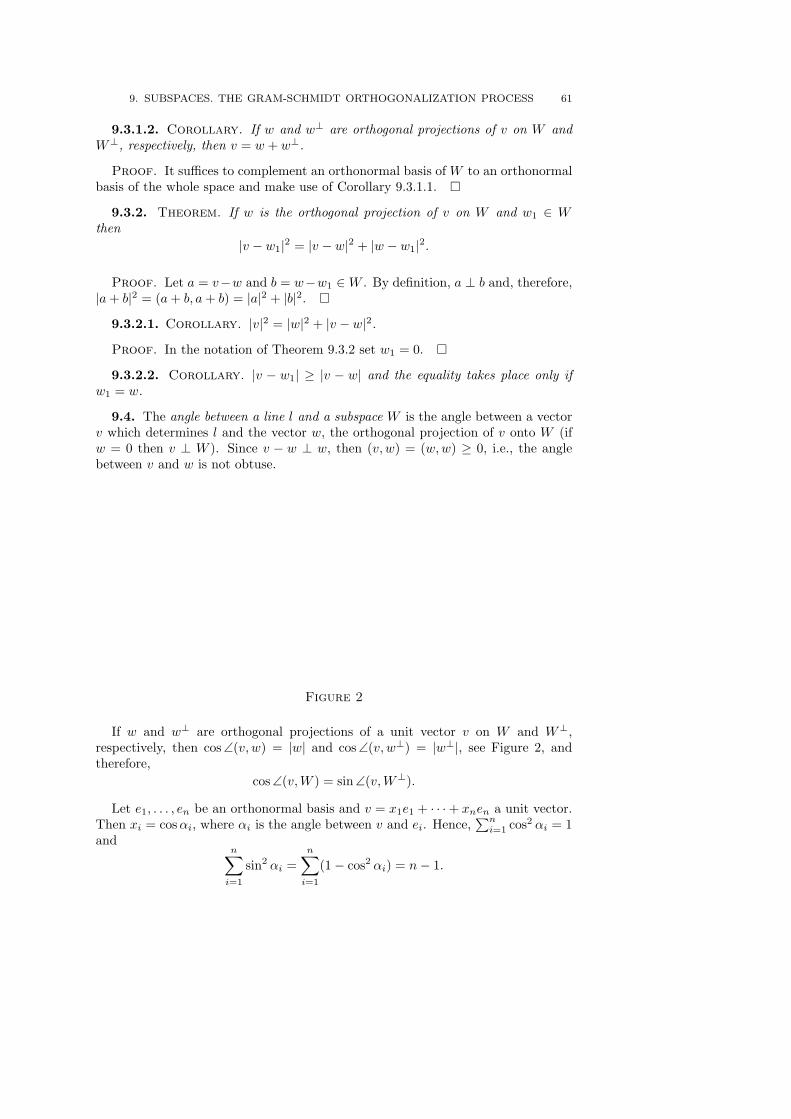
9. SUBSPACES. THE GRAM-SCHMIDT ORTHOGONALIZATION PROCESS 61
9.3.1.2. Corollary. If w and w⊥ are orthogonal projections of v on W andW⊥, respectively, then v = w + w⊥.
Proof. It suffices to complement an orthonormal basis of W to an orthonormalbasis of the whole space and make use of Corollary 9.3.1.1. ¤
9.3.2. Theorem. If w is the orthogonal projection of v on W and w1 ∈ Wthen
|v − w1|2 = |v − w|2 + |w − w1|2.
Proof. Let a = v−w and b = w−w1 ∈W . By definition, a ⊥ b and, therefore,|a+ b|2 = (a+ b, a+ b) = |a|2 + |b|2. ¤
9.3.2.1. Corollary. |v|2 = |w|2 + |v − w|2.
Proof. In the notation of Theorem 9.3.2 set w1 = 0. ¤
9.3.2.2. Corollary. |v − w1| ≥ |v − w| and the equality takes place only ifw1 = w.
9.4. The angle between a line l and a subspace W is the angle between a vectorv which determines l and the vector w, the orthogonal projection of v onto W (ifw = 0 then v ⊥ W ). Since v − w ⊥ w, then (v, w) = (w,w) ≥ 0, i.e., the anglebetween v and w is not obtuse.
Figure 2
If w and w⊥ are orthogonal projections of a unit vector v on W and W⊥,respectively, then cos ∠(v, w) = |w| and cos ∠(v, w⊥) = |w⊥|, see Figure 2, andtherefore,
cos ∠(v,W ) = sin ∠(v,W⊥).
Let e1, . . . , en be an orthonormal basis and v = x1e1 + · · ·+ xnen a unit vector.Then xi = cosαi, where αi is the angle between v and ei. Hence,
∑ni=1 cos2 αi = 1
andn∑
i=1
sin2 αi =n∑
i=1
(1− cos2 αi) = n− 1.
62 LINEAR SPACES
Theorem. Let e1, . . . , ek be an orthonormal basis of a subspace W ⊂ V andαi the angle between v and ei and α the angle between v and W . Then cos2 α =∑ki=1 cos2 αi.
Proof. Let us complement the basis e1, . . . , ek to a basis e1, . . . , en of V . Thenv = x1e1 + · · · + xnen, where xi = cosαi for i = 1, . . . , k, and the projection of vonto W is equal to x1e1 + · · ·+ xkek = w. Hence,
cos2 α = |w|2 = x21 + · · ·+ x2
k = cos2 α1 + · · ·+ cos2 αk. ¤
9.5. Theorem ([Nisnevich, Bryzgalov, 1953]). Let e1, . . . , en be an orthogonalbasis of V , and d1, . . . , dn the lengths of the vectors e1, . . . , en. An m-dimensionalsubspace W ⊂ V such that the projections of these vectors on W are of equal lengthexists if and only if
d2i (d−21 + · · ·+ d−2
n ) ≥ m for i = 1, . . . , n.
Proof. Take an orthonormal basis in W and complement it to an orthonormalbasis ε1, . . . , εn of V . Let (x1i, . . . , xni) be the coordinates of ei with respect tothe basis ε1, . . . , εn and yki = xki/di. Then
∥∥yki∥∥ is an orthogonal matrix and the
length of the projection of ei on W is equal to d if and only if
(1) y21i + · · ·+ y2
mi = (x21i + · · ·+ x2
mi)d−2i = d2d−2
i .
If the required subspace W exists then d ≤ di and
m =m∑
k=1
n∑
i=1
y2ki =
n∑
i=1
m∑
k=1
y2ki = d2(d−2
1 + · · ·+ d−2n ) ≤ d2
i (d−21 + · · ·+ d−2
n ).
Now, suppose that m ≤ d2i (d−21 + · · · + d−2
n ) for i = 1, . . . , n and construct anorthogonal matrix
∥∥yki∥∥n
1with property (1), where d2 = m(d−2
1 + · · ·+d−2n )−1. We
can now construct the subspace W in an obvious way.Let us prove by induction on n that if 0 ≤ βi ≤ 1 for i = 1, . . . , n and β1 + · · ·+
βn = m, then there exists an orthogonal matrix∥∥yki
∥∥n1
such that y21i+· · ·+y2
mi = βi.For n = 1 the statement is obvious. Suppose the statement holds for n − 1 andprove it for n. Consider two cases:
a) m ≤ n/2. We can assume that β1 ≥ · · · ≥ βn. Then βn−1 + βn ≤ 2m/n ≤ 1and, therefore, there exists an orthogonal matrix A =
∥∥aki∥∥n−1
1such that a2
1i +· · · + a2
mi = βi for i = 1, . . . , n − 2 and a21,n−1 + · · · + a2
m,n−1 = βn−1 + βn. Thenthe matrix
∥∥yki∥∥n
1=
a11 . . . a1,n−2 α1a1,n−1 −α2a1,n−1
... · · · ......
...an−1,1 . . . an−1,n−2 α1an−1,n−1 −α2an−1,n−1
0 . . . 0 α2 α1
,
10. COMPLEXIFICATION AND REALIFICATION. UNITARY SPACES 63
where α1 =√
βn−1
βn−1 + βnand α2 =
√βn
βn−1 + βn, is orthogonal with respect to its
columns; besides,
m∑
k=1
y2ki = βi for i = 1, . . . , n− 2
y21,n−1 + · · ·+ y2
m,n−1 = α21(βn−1 + βn) = βn−1,
y21n + · · ·+ y2
mn = βn
b) Let m > n/2. Then n−m < n/2, and, therefore, there exists an orthogonalmatrix
∥∥yki∥∥n
1such that y2
m+1,i + · · · + y2n,i = 1 − βi for i = 1, . . . , n; hence,
y21i + · · ·+ y2
mi = βi. ¤9.6.1. Theorem. Suppose a set of k-dimensional subspaces in a space V is
given so that the intersection of any two of the subspaces is of dimension k − 1.Then either all these subspaces have a common (k− 1)-dimensional subspace or allof them are contained in the same (k + 1)-dimensional subspace.
Proof. Let V k−1ij = V ki ∩ V kj and Vijl = V ki ∩ V kj ∩ V kl . First, let us prove that
if V123 6= V k−112 then V k3 ⊂ V k1 + V k2 . Indeed, if V123 6= V k−1
12 then V k−112 and V k−1
23
are distinct subspaces of V k2 and the subspace V123 = V k−112 ∩ V k−1
23 is of dimensionk− 2. In V123, select a basis ε and complement it by vectors e13 and e23 to bases ofV13 and V23, respectively. Then V3 = Span(e13, e23, ε), where e13 ∈ V1 and e23 ∈ V2.
Suppose the subspaces V k1 , V k2 and V k3 have no common (k − 1)-dimensionalsubspace, i.e., the subspaces V k−1
12 and V k−123 do not coincide. The space Vi could
not be contained in the subspace spanned by V1, V2 and V3 only if V12i = V12 andV23i = V23. But then dimVi ≥ dim(V12 + V23) = k + 1 which is impossible. ¤
If we consider the orthogonal complements to the given subspaces we get thetheorem dual to Theorem 9.6.1.
9.6.2. Theorem. Let a set of m-dimensional subspaces in a space V be givenso that any two of them are contained in a (m + 1)-dimensional subspace. Theneither all of them belong to an (m+ 1)-dimensional subspace or all of them have acommon (m− 1)-dimensional subspace.
Problems
9.1. In an n-dimensional space V , there are given m-dimensional subspaces Uand W so that u ⊥W for some u ∈ U \ 0. Prove that w ⊥ U for some w ∈W \ 0.
9.2. In an n-dimensional Euclidean space two bases x1, . . . , xn and y1, . . . , yn aregiven so that (xi, xj) = (yi, yj) for all i, j. Prove that there exists an orthogonaloperator U which sends xi to yi.
10. Complexification and realification. Unitary spaces
10.1. The complexification of a linear space V over R is the set of pairs (a, b),where a, b ∈ V , with the following structure of a linear space over C:
(a, b) + (a1, b1) = (a+ a1, b+ b1)
(x+ iy)(a, b) = (xa− yb, xb+ ya).
64 LINEAR SPACES
Such pairs of vectors can be expressed in the form a+ ib. The complexification ofV is denoted by V C.
To an operator A : V −→ V there corresponds an operator AC : V C −→ V C givenby the formula AC(a+ib) = Aa+iAb. The operator AC is called the complexificationof A.
10.2. A linear space V over C is also a linear space over R. The space over Robtained is called a realification of V . We will denote it by VR.
A linear map A : V −→W over C can be considered as a linear map AR : VR −→WR over R. The map AR is called the realification of the operator A.
If e1, . . . , en is a basis of V over C then e1, . . . , en, ie1, . . . , ien is a basis of VR. Itis easy to verify that if A = B+ iC is the matrix of a linear map A : V −→W withrespect to bases e1, . . . , en and ε1, . . . , εm and the matrices B and C are real, thenthe matrix of the linear map AR with respect to the bases e1, . . . , en, ie1, . . . , ien
and ε1, . . . , εm, iε1, . . . , iεm is of the form(B −CC B
).
Theorem. If A : V −→ V is a linear map over C then detAR = | detA|2.
Proof.
(I 0−iI I
)(B −CC B
)(I 0iI I
)=
(B − iC −C
0 B + iC
).
Therefore, detAR = detA · det A = | detA|2. ¤10.3. Let V be a linear space over C. An Hermitian product in V is a map
V × V −→ C which to a pair of vectors x, y ∈ V assigns a complex number (x, y)and has the following properties:
1) (x, y) = (y, x);2) (αx+ βy, z) = α(x, z) + β(y, z);3) (x, x) is a positive real number for any x 6= 0.A space V with an Hermitian product is called an Hermitian (or unitary) space.
The standard Hermitian product in Cn is of the form x1y1 + · · ·+ xnyn.A linear operator A∗ is called the Hermitian adjoint to A if
(Ax, y) = (x,A∗y) = (A∗y, x).
(Physicists often denote the Hermitian adjoint by A+.)Let
∥∥aij∥∥n
1and
∥∥bij∥∥n
1be the matrices of A and A∗ with respect to an orthonor-
mal basis. Thenaij = (Aej , ei) = (A∗ej , ei) = bji.
A linear operator A is called unitary if (Ax,Ay) = (x, y), i.e., a unitary operatorpreserves the Hermitian product. If an operator A is unitary then
(x, y) = (Ax,Ay) = (x,A∗Ay).
Therefore, A∗A = I = AA∗, i.e., the rows and the columns of the matrix of Aconstitute an orthonormal systems of vectors.
A linear operator A is called Hermitian (resp. skew-Hermitian ) if A∗ = A (resp.A∗ = −A). Clearly, a linear operator is Hermitian if and only if its matrix A is
10. COMPLEXIFICATION AND REALIFICATION. UNITARY SPACES 65
Hermitian with respect to an orthonormal basis, i.e., AT
= A; and in this case itsmatrix is Hermitian with respect to any orthonormal basis.
Hermitian matrices are, as a rule, analogues of real symmetric matrices in thecomplex case. Sometimes complex symmetric or skew-symmetric matrices (thatis such that satisfy the condition AT = A or AT = −A, respectively) are alsoconsidered.
10.3.1. Theorem. Let A be a complex operator such that (Ax, x) = 0 for allx. Then A = 0.
Proof. Let us write the equation (Ax, x) = 0 twice: for x = u+v and x = u+iv.Taking into account that (Av, v) = (Au, u) = 0 we get (Av, u) + (Au, v) = 0 andi(Av, u)− i(Au, v) = 0. Therefore, (Au, v) = 0 for all u, v ∈ V . ¤
Remark. For real operators the identity (Ax, x) = 0 means that A is a skew-symmetric operator (cf. Theorem 21.1.2).
10.3.2. Theorem. Let A be a complex operator such that (Ax, x) ∈ R for anyx. Then A is an Hermitian operator.
Proof. Since (Ax, x) = (Ax, x) = (x,Ax), then
((A−A∗)x, x) = (Ax, x)− (A∗x, x) = (Ax, x)− (x,Ax) = 0.
By Theorem 10.3.1 A−A∗ = 0. ¤10.3.3. Theorem. Any complex operator is uniquely representable in the form
A = B + iC, where B and C are Hermitian operators.
Proof. If A = B + iC, where B and C are Hermitian operators, then A∗ =B∗ − iC∗ = B − iC and, therefore 2B = A + A∗ and 2iC = A − A∗. It is easy toverify that the operators 1
2 (A+A∗) and 12i (A−A∗) are Hermitian. ¤
Remark. An operator iC is skew-Hermitian if and only if the operator C isHermitian and, therefore, any operator A is uniquely representable in the form ofa sum of an Hermitian and a skew-Hermitian operator.
An operator A is called normal if A∗A = AA∗. It is easy to verify that unitary,Hermitian and skew-Hermitian operators are normal.
10.3.4. Theorem. An operator A = B + iC, where B and C are Hermitianoperators, is normal if and only if BC = CB.
Proof. Since A∗ = B∗−iC∗ = B−iC, then A∗A = B2 +C2 +i(BC−CB) andAA∗ = B2 + C2 − i(BC − CB). Therefore, the equality A∗A = AA∗ is equivalentto the equality BC − CB = 0. ¤
10.4. If V is a linear space over R, then to define on V a structure of a linearspace over C it is necessary to determine the operation J of multiplication by i,i.e., Jv = iv. This linear map J : V −→ V should satisfy the following property
J2v = i(iv) = −v, i.e., J2 = −I.It is also clear that if in a space V over R such a linear operator J is given thenwe can make V into a space over C if we define the multiplication by a complexnumber a+ ib by the formula
(a+ ib)v = av + bJv.
66 LINEAR SPACES
In particular, the dimension of V in this case must be even.Let V be a linear space over R. A linear (over R) operator J : V −→ V is called
a complex structure on V if J2 = −I.The eigenvalues of the operator J : V −→ V are purely imaginary and, therefore,
for a more detailed study of J we will consider the complexification V C of V . Noticethat the multiplication by i in V C has no relation whatsoever with neither thecomplex structure J on V or its complexification JC acting in V C.
Theorem. V C = V+ ⊕ V−, where
V+ = Ker(JC − iI) = Im(JC + iI)
andV− = Ker(JC + iI) = Im(JC − iI).
Proof. Since (JC − iI)(JC + iI) = (J2)C + I = 0, it follows that Im(JC +iI) ⊂ Ker(JC − iI). Similarly, Im(JC − iI) ⊂ Ker(JC + iI). On the other hand,−i(JC + iI) + i(JC − iI) = 2I and, therefore, V C ⊂ Im(JC + iI) + Im(JC − iI).Since Ker(JC − iI) ∩Ker(JC + iI) = 0, we get the required conclusion. ¤
Remark. Clearly, V+ = V−.
Problems
10.1. Express the characteristic polynomial of the matrix AR in terms of thecharacteristic polynomial of A.
10.2. Consider an R-linear map of C into itself given by Az = az + bz, wherea, b ∈ C. Prove that this map is not invertible if and only if
|a| = |b|.
10.3. Indicate in Cn a complex subspace of dimension [n/2] on which the qua-dratic form B(x, y) = x1y1 + · · ·+ xnyn vanishes identically.
Solutions
5.1. The orthogonal complement to the space of traceless matrices is one-dimensional; it contains both matrices I and AT .
5.2. Let A1, . . . , Am and B1, . . . , Bk be the rows of the matrices A and B.Then
Span(A1, . . . , Am)⊥ ⊂ Span(B1, . . . , Bk)⊥;
hence, Span(B1, . . . , Bk) ⊂ Span(A1, . . . , Am), i.e., bij =∑cipapj .
5.3. If a vector (w1, . . . , wn) belongs to an orthant that does not contain thevectors ±v, then viwi > 0 and vjwj < 0 for certain indices i and j. If we preservethe sign of the coordinate wi (resp. wj) but enlarge its absolute value then theinner product (v, w) will grow (resp. decrease) and, therefore it can be made zero.
5.4. Let us express the bilinear function x∗(y) in the form xByT . By hypothesisthe conditions xByT = 0 and yBxT = 0 are equivalent. Besides, yBxT = xBT yT .Therefore, ByT = λ(y)BT yT . If vectors y and y1 are proportional then λ(y) =
SOLUTIONS 67
λ(y1). If the vectors y and y1 are linearly independent then the vectors BT yT andBT yT1 are also linearly independent and, therefore, the equalities
λ(y + y1)(BT yT +BT yT1 ) = B(yT + yT1 ) = λ(y)BT yT + λ(y1)BT yT1
imply λ(y) = λ(y1). Thus, x∗(y) = B(x, y) and B(x, y) = λB(y, x) = λ2B(x, y)and, therefore, λ = ±1.
6.1. By Theorem 6.1
dim(ImAk ∩KerA) = dim KerAk+1 − dim KerAk for any k.
Therefore,
n∑
k=1
dim(ImAk ∩KerA) = dim KerAn+1 − dim KerA.
To prove the second equality it suffices to notice that
dim ImAp = dimV − dim KerAp,
where V is the space in which A acts.7.1. We may assume that e1, . . . , ek (k ≤ n) is a basis of Span(e1, . . . , em). Then
ek+1 + λ1e1 + · · ·+ λkek = 0 and ek+2 + µ1e1 + · · ·+ µkek = 0.
Multiply these equalities by 1+∑µi and −(1+
∑λi), respectively, and add up the
obtained equalities. (If 1 +∑µi = 0 or 1 +
∑λi = 0 we already have the required
equality.)7.2. Let us carry out the proof by induction on m. For m ≤ n+ 1 the statement
is obvious. Let m ≥ n + 2. Then there exist numbers α1, . . . , αm not all equal tozero such that
∑αivi = 0 and
∑αi = 0 (see Problem 7.1). Therefore,
x =∑
tivi + λ∑
αivi =∑
t′ivi,
where t′i = ti + λαi and∑t′i =
∑ti = 1. It remains to find a number λ so that all
numbers ti + λαi are nonnegative and at least one of them is zero. The set
λ ∈ R | ti + λαi ≥ 0 for i = 1, . . . ,m
is closed, nonempty (it contains zero) and is bounded from below (and above) sinceamong the numbers αi there are positive (and negative) ones; the minimal numberλ from this set is the desired one.
7.3. Suppose A is not invertible. Then there exist numbers λ1, . . . , λn not allequal to zero such that
∑i λiaik = 0 for k = 1, . . . , n. Let λs be the number among
λ1, . . . , λn whose absolute value is the greatest (for definiteness sake let s = 1).Since
λ1a11 + λ2a12 + · · ·+ λna1n = 0,
then
|λ1a11| = |λ2a12 + · · ·+ λna1n| ≤ |λ2a12|+ · · ·+ |λna1n|≤ |λ1| (|a12|+ · · ·+ |a1n|) < |λ1| · |a11|.
68 LINEAR SPACES
Contradiction.7.4. a) Suppose that the vectors e1, . . . , ek are linearly dependent for k < n+ 1.
We may assume that this set of vectors is minimal, i.e., λ1e1 + · · ·+λkek = 0, whereall the numbers λi are nonzero. Then
0 = (en+1,∑λiei) =
∑λi(en+1, ei), where (en+1, ei) < 0.
Therefore, among the numbers λi there are both positive and negative ones. Onthe other hand, if
λ1e1 + · · ·+ λpep = λ′p+1ep+1 + · · ·+ λ′kek,
where all numbers λi, λ′j are positive, then taking the inner product of this equalitywith the vector in its right-hand side we get a negative number in the left-hand sideand the inner product of a nonzero vector by itself, i.e., a nonnegative number, inthe right-hand side.
b) Suppose that vectors e1, . . . , en+2 in Rn are such that (ei, ej) < 0 for i 6= j.On the one hand, if α1e1 + · · ·+ αn+2en+2 = 0 then all the numbers αi are of thesame sign (cf. solution to heading a). On the other hand, we can select the numbersα1, . . . , αn+2 so that
∑αi = 0 (see Problem 7.1). Contradiction.
8.1. Let
X =
x1 1...
...xn 1
, Y =
(1 . . . 1y1 . . . yn
).
Then∥∥aij
∥∥n1
= XY .8.2. Let e1 be a vector that generates ImA. Let us complement it to a basis
e1, . . . , en. The matrix A with respect to this basis is of the form
A =
a1 . . . an0 . . . 0... · · · ...0 . . . 0
.
Therefore, trA = a1 and |A+ I| = 1 + a1.8.3. It suffices to show that KerA∗ ∩ ImA = 0. If A∗v = 0 and v = Aw, then
(v, v) = (Aw, v) = (w,A∗v) = 0 and, therefore, v = 0.8.4. The rows of the matrix (C,D) are linear combinations of the rows of the
matrix (A,B) and, therefore, (C,D) = X(A,B) = (XA,XB), i.e., D = XB =(CA−1)B.
8.5. Let ri = rankAi and r = rank(A1 + A2). Then dimVi = dimWi = riand dim(V1 + V2) = dim(W1 + W2) = r. The equality r1 + r2 = r means thatdim(V1 + V2) = dimV1 + dimV2, i.e., V1 ∩ V2 = 0. Similarly, W1 ∩W2 = 0.
8.6. The equality BTA = 0 means that the columns of the matrices A and B arepair-wise orthogonal. Therefore, the space spanned by the columns of A has onlyzero intersection with the space spanned by the columns of B. It remains to makeuse of the result of Problem 8.5.
8.7. Suppose A and B are matrices of order 2m+ 1. By Sylvester’s inequality,
rankA+ rankB ≤ rankAB + 2m+ 1 = 2m+ 1.
SOLUTIONS 69
Therefore, either rankA ≤ m or rankB ≤ m. If rankA ≤ m then rankAT =rankA ≤ m; hence,
rank(A+AT ) ≤ rankA+ rankAT ≤ 2m < 2m+ 1.
8.8. We may assume that a12 6= 0. Let Ai be the ith row of A. Let us provethat a21Ai = a2iA1 + ai1A2, i.e.,
(1) a12aij + a1ja2i + a1iaj2 = 0.
The identity (1) is skew-symmetric with respect to i and j and, therefore, wecan assume that i < j, see Figure 3.
Figure 3
Only the factor aj2 is negative in (1) and, therefore, (1) is equivalent to Ptolemy’stheorem for the quadrilateral X1X2XiXj .
9.1. Let U1 be the orthogonal complement of u in U . Since
dimU⊥1 + dimW = n− (m− 1) +m = n+ 1,
then dim(U⊥1 ∩W ) ≥ 1. If w ∈W ∩U⊥1 then w ⊥ U1 and w ⊥ u; therefore, w ⊥ U .9.2. Let us apply the orthogonalization process with the subsequent normaliza-
tion to vectors x1, . . . , xn. As a result we get an orthonormal basis e1, . . . , en. Thevectors x1, . . . , xn are expressed in terms of e1, . . . , en and the coefficients onlydepend on the inner products (xi, xj). Similarly, for the vectors y1, . . . , yn we getan orthonormal basis ε1, . . . , εn. The map that sends ei to εi (i = 1, . . . , n) is therequired one.
10.1. det(λI −AR) = |det(λI −A)|2.10.2. Let a = a1+ia2, b = b1+ib2, where ai, bi ∈ R. The matrix of the given map
with respect to the basis 1, i is equal to(a1 + b1 −a2 + b2a2 + b2 a1 − b1
)and its determinant
is equal to |a|2 − |b|2.10.3. Let p = [n/2]. The complex subspace spanned by the vectors e1 + ie2,
e3 + ie4, . . . , e2p−1 + ie2p possesses the required property.
70 LINEAR SPACESCHAPTER III
CANONICAL FORMS OF MATRICES
AND LINEAR OPERATORS
11. The trace and eigenvalues of an operator
11.1. The trace of a square matrix A is the sum of its diagonal elements; it isdenoted by trA. It is easy to verify that
trAB =∑
i,j
aijbji = trBA.
Therefore,trPAP−1 = trP−1PA = trA,
i.e., the trace of the matrix of a linear operator does not depend on the choice of abasis.
The equality trABC = trACB is not always true. For instance, take A =(0 10 0
), B =
(1 00 0
)and C =
(0 01 0
); then ABC = 0 and ACB =
(1 00 0
).
For the trace of an operator in a Euclidean space we have the following usefulformula.
Theorem. Let e1, . . . , en be an orthonormal basis. Then
trA =n∑
i=1
(Aei, ei).
Proof. Since Aei =∑j aijej , then (Aei, ei) = aii. ¤
Remark. The trace of an operator is invariant but the above definition of thetrace makes use of a basis and, therefore, is not invariant. One can, however, givean invariant definition of the trace of an operator (see 27.2).
11.2. A nonzero vector v ∈ V is called an eigenvector of the linear operatorA : V → V if Av = λv and this number λ is called an eigenvalue of A. Fix λ andconsider the equation Av = λv, i.e., (A − λI)v = 0. This equation has a nonzerosolution v if and only if |A− λI| = 0. Therefore, the eigenvalues of A are roots ofthe polynomial p(λ) = |λI −A|.
The polynomial p(λ) is called the characteristic polynomial of A. This polyno-mial only depends on the operator itself and does not depend on the choice of thebasis (see 7.1).
Theorem. If Ae1 = λ1e1, . . . , Aek = λkek and the numbers λ1, . . . , λk aredistinct, then e1, . . . , ek are linearly independent.
Proof. Assume the contrary. Selecting a minimal linearly independent set ofvectors we can assume that ek = α1e1 + · · · + αk−1ek−1, where α1 . . . αk−1 6= 0and the vectors e1, . . . , ek−1 are linearly independent. Then Aek = α1λ1e1 + · · ·+αk−1λk−1ek−1 and Aek = λkek = α1λke1 + · · · + αk−1λkek−1. Hence, λ1 = λk.Contradiction. ¤
Typeset by AMS-TEX
11. THE TRACE AND EIGENVALUES OF AN OPERATOR 71
Corollary. If the characteristic polynomial of an operator A over C has nomultiple roots then the eigenvectors of A constitute a basis.
11.3. A linear operator A possessing a basis of eigenvectors is said to be adiagonalizable or semisimple. If X is the matrix formed by the columns of thecoordinates of eigenvectors x1, . . . , xn and λi an eigenvalue corresponding to xi,then AX = XΛ, where Λ = diag(λ1, . . . , λn). Therefore, X−1AX = Λ.
The converse is also true: if X−1AX = diag(λ1, . . . , λn), then λ1, . . . , λn areeigenvalues of A and the columns of X are the corresponding eigenvectors.
Over C only an operator with multiple eigenvalues may be nondiagonalizable andsuch operators constitute a set of measure zero. All normal operators (see 17.1)are diagonalizable over C. In particular, all unitary and Hermitian operators arediagonalizable and there are orthonormal bases consisting of their eigenvectors.This can be easily proved in a straightforward way as well with the help of thefact that for a unitary or Hermitian operator A the inclusion AW ⊂ W impliesAW⊥ ⊂W⊥.
The absolute value of an eigenvalue of a unitary operator A is equal to 1 since|Ax| = |x|. The eigenvalues of an Hermitian operator A are real since (Ax, x) =(x,Ax) = (Ax, x).
Theorem. For an orthogonal operator A there exists an orthonormal basis withrespect to which the matrix of A is of the block-diagonal form with blocks ±1 or(
cosϕ − sinϕsinϕ cosϕ
).
Proof. If ±1 is an eigenvalue of A we can make use of the same arguments asfor the complex case and therefore, let us assume that the vectors x and Ax arenot parallel for all x. The function ϕ(x) = ∠(x,Ax) — the angle between x andAx — is continuous on a compact set, the unit sphere.
Let ϕ0 = ∠(x0, Ax0) be the minimum of ϕ(x) and e the vector parallel to thebisector of the angle between x0 and Ax0.
Thenϕ0 ≤ ∠(e,Ae) ≤ ∠(e,Ax0) + ∠(Ax0, Ae) =
ϕ0
2+ϕ0
2
and, therefore, Ae belongs to the plane Span(x0, e). This plane is invariant withrespect to A since Ax0, Ae ∈ Span(x0, e). An orthogonal transformation of a planeis either a rotation or a symmetry through a straight line; the eigenvalues of asymmetry, however, are equal to ±1 and, therefore, the matrix of the restriction of
A to Span(x0, e) is of the form(
cosϕ − sinϕsinϕ cosϕ
), where sinϕ 6= 0. ¤
11.4. The eigenvalues of the tridiagonal matrix
J =
a1 −b1 0 . . . 0 0−c1 a2 −b2 . . . 0 0
0 −c2 a3 . . . 0 0...
......
. . . . . . . . ....
0 0 0 . . . an−2 −bn−2 00 0 0 . . . −cn−2 an−1 −bn−1
0 0 0 . . . 0 −cn−1 an
, where bici > 0,
72 CANONICAL FORMS OF MATRICES AND LINEAR OPERATORS
have interesting properties. They are real and of multiplicity one. For J =∥∥aij
∥∥n1,
consider the sequence of polynomials
Dk(λ) = |λδij − aij |k1 , D0(λ) = 1.
Clearly, Dn(λ) is the characteristic polynomial of J . These polynomials satisfy arecurrent relation
(1) Dk(λ) = (λ− ak)Dk−1(λ)− bk−1ck−1Dk−2(λ)
(cf. 1.6) and, therefore, the characteristic polynomial Dn(λ) depends not on thenumbers bk, ck themselves, but on their products. By replacing in J the elementsbk and ck by
√bkck we get a symmetric matrix J1 with the same characteristic
polynomial. Therefore, the eigenvalues of J are real.A symmetric matrix has a basis of eigenvectors and therefore, it remains to
demonstrate that to every eigenvalue λ of J1 there corresponds no more than oneeigenvector (x1, . . . , xn). This is also true even for J , i.e without the assumptionthat bk = ck. Since
(λ− a1)x1 − b1x2 = 0
−c1x1 + (λ− a2)x2 − b2x3 = 0
. . . . . . . . . . . . . . .
−cn−2xn−2 + (λ− an−1)xn−1 − bn−1xn = 0
−cn−1xn−1 + (λ− an)xn = 0,
it follows that the change
y1 = x1, y2 = b1x2, . . . , yk = b1 . . . bk−1xk,
yieldsy2 = (λ− a1)y1
y3 = (λ− a2)y2 − c1b1y1
. . . . . . . . . . . . . . . . . .
yn = (λ− an−1)yn−1 − cn−2bn−2yn−2.
These relations for yk coincide with relations (1) for Dk and, therefore, if y1 = c =cD0(λ) then yk = cDk(λ). Thus the eigenvector (x1, . . . , xk) is uniquely determinedup to proportionality.
11.5. Let us give two examples of how to calculate eigenvalues and eigenvectors.First, we observe that if λ is an eigenvalue of a matrix A and f an arbitrarypolynomial, then f(λ) is an eigenvalue of the matrix f(A). This follows from thefact that f(λI)− f(A) is divisible by λI −A.
a) Consider the matrix
P =
0 0 0 . . . 0 0 11 0 0 . . . 0 0 00 1 0 . . . 0 0 0...
......
. . . . . ....
...0 0 0 . . . 0 1 0
.
11. THE TRACE AND EIGENVALUES OF AN OPERATOR 73
Since Pek = ek+1, then P sek = ek+s and, therefore, Pn = I, where n is the orderof the matrix. It follows that the eigenvalues are roots of the equation xn = 1. Setε = exp(2πi/n). Let us prove that the vector us =
∑nk=1 ε
ksek (s = 1, . . . , n) is aneigenvector of P corresponding to the eigenvalue ε−s. Indeed,
Pus =∑
εksPek =∑
εksek+1 =∑
ε−s(εs(k+1)ek+1) = ε−sus.
b) Consider the matrix
A =
0 1 0 . . . 0
0 0 1. . . 0
......
. . . . . ....
0 0 0 . . . 1p1 p2 p3 . . . pn
.
Let x be the column (x1, . . . , xn)T . The equation Ax = λx can be rewritten in theform
x2 = λx1, x3 = λx2, . . . , xn = λxn−1, p1x1 + p2x2 + · · ·+ pnxn = λxn.
Therefore, the eigenvectors of A are of the form
(α, λα, λ2α, . . . , λn−1α), where p1 + p2λ+ · · ·+ pnλn−1 = λn.
11.6. We already know that trAB = trBA. It turns out that a stronger state-ment is true: the matrices AB and BA have the same characteristic polynomials.
Theorem. Let A and B be n×n-matrices. Then the characteristic polynomialsof AB and BA coincide.
Proof. If A is invertible then
|λI −AB| = |A−1(λI −AB)A| = |λI −BA|.For a noninvertible matrix A the equality |λI −AB| = |λI −BA| can be proved bypassing to the limit. ¤
Corollary. If A and B are m×n-matrices, then the characteristic polynomialsof ABT and BTA differ by the factor λn−m.
Proof. Complement the matrices A and B by zeros to square matrices of equalsize. ¤
11.7.1. Theorem. Let the sum of the elements of every column of a squarematrix A be equal to 1, and let the column (x1, . . . , xn)T be an eigenvector of Asuch that x1 + · · · + xn 6= 0. Then the eigenvalue corresponding to this vector isequal to 1.
Proof. Adding up the equalities∑a1jxj = λx1, . . . ,
∑anjxj = λxn we get∑
i,j aijxj = λ∑j xj . But
∑
i,j
aijxj =∑
j
(xj
∑
i
aij
)=
∑xj
since∑i aij = 1. Thus,
∑xj = λ
∑xj , where
∑xj 6= 0. Therefore, λ = 1. ¤
74 CANONICAL FORMS OF MATRICES AND LINEAR OPERATORS
11.7.2. Theorem. If the sum of the absolute values of the elements of everycolumn of a square matrix A does not exceed 1, then all its eigenvalues do not exceed1.
Proof. Let (x1, . . . , xn) be an eigenvector corresponding to an eigenvalue λ.Then
|λxi| = |∑
aijxj | ≤∑|aij ||xj |, i = 1, . . . , n.
Adding up these inequalities we get
|λ|∑|xi| ≤
∑
i,j
|aij ||xj | =∑
j
(|xj |
∑
i
|aij |)≤
∑
j
|xj |
since∑i |aij | ≤ 1. Dividing both sides of this inequality by the nonzero number∑ |xj | we get |λ| ≤ 1. ¤
Remark. Theorem 11.7.2 remains valid also when certain of the columns of Aare zero ones.
11.7.3. Theorem. Let A =∥∥aij
∥∥n1
, Sj =∑ni=1 |aij |; then
∑nj=1 S
−1j |ajj | ≤
rankA and the summands corresponding to zero values of Sj can be replaced byzeros.
Proof. Multiplying the columns of A by nonzero numbers we can always makethe numbers Sj for the new matrix to be either 0 or 1 and, besides, ajj ≥ 0.The rank of the matrix is not effected by these transformations. Applying Theo-rem 11.7.2 to the new matrix we get
∑|ajj | =
∑ajj = trA =
∑λi ≤
∑|λi| ≤ rankA. ¤
Problems
11.1. a) Are there real matrices A and B such that AB −BA = I?b) Prove that if AB −BA = A then |A| = 0.11.2. Find the eigenvalues and the eigenvectors of the matrix A =
∥∥aij∥∥n
1, where
aij = λi/λj .11.3. Prove that any square matrix A is the sum of two invertible matrices.11.4. Prove that the eigenvalues of a matrix continuously depend on its elements.
More precisely, let A =∥∥aij
∥∥n1
be a given matrix. For any ε > 0 there exists δ > 0such that if |aij−bij | < δ and λ is an eigenvalue of A, then there exists an eigenvalueµ of B =
∥∥bij∥∥n
1such that |λ− µ| < ε.
11.5. The sum of the elements of every row of an invertible matrix A is equal tos. Prove that the sum of the elements of every row of A−1 is equal to 1/s.
11.6. Prove that if the first row of the matrix S−1AS is of the form (λ, 0, 0, . . . , 0)then the first column of S is an eigenvector of A corresponding to the eigenvalue λ.
11.7. Let f(λ) = |λI − A|, where A is a matrix of order n. Prove that f ′(λ) =∑ni=1 |λI−Ai|, where Ai is the matrix obtained from A by striking out the ith row
and the ith column.11.8. Let λ1, . . . , λn be the eigenvalues of a matrix A. Prove that the eigenvalues
of adjA are equal to∏i 6=1 λi, . . . ,
∏i6=n λi.
12. THE JORDAN CANONICAL (NORMAL) FORM 75
11.9. A vector x is called symmetric (resp. skew-symmetric) if its coordinatessatisfy (xi = xn−i) (resp. (xi = −xn−i)). Let a matrix A =
∥∥aij∥∥n
0be cen-
trally symmetric, i.e., ai,j = an−i,n−j . Prove that among the eigenvectors of Acorresponding to any eigenvalue there is either a nonzero symmetric or a nonzeroskew-symmetric vector.
11.10. The elements ai,n−i+1 = xi of a complex n× n-matrix A can be nonzero,whereas the remaining elements are 0. What condition should the set x1, . . . , xnsatisfy for A to be diagonalizable?
11.11 ([Drazin, Haynsworth, 1962]). a) Prove that a matrix A has m linearlyindependent eigenvectors corresponding to real eigenvalues if and only if there existsa nonnegative definite matrix S of rankm such that AS = SA∗.
b) Prove that a matrix A has m linearly independent eigenvectors correspondingto eigenvalues λ such that |λ| = 1 if and only if there exists a nonnegative definitematrix S of rankm such that ASA∗ = S.
12. The Jordan canonical (normal) form
12.1. Let A be the matrix of an operator with respect to a basis e; then P−1APis the matrix of the same operator with respect to the basis eP . The matrices Aand P−1AP are called similar. By selecting an appropriate basis we can reduce thematrix of an operator to a simpler form: to a Jordan normal form, cyclic form, toa matrix with equal elements on the main diagonal, to a matrix all whose elementson the main diagonal, except one, are zero, etc.
One might think that for a given real matrix A the set of real matrices of theform P−1AP |P , where P is a complex matrix is “broader” than the the set of realmatrices of the form P−1AP |P , where P is a real matrix. This, however, is not so.
Theorem. Let A and B be real matrices and A = P−1BP , where P is a complexmatrix. Then A = Q−1BQ for some real matrix Q.
Proof. We have to demonstrate that if among the solutions of the equation
(1) XA = BX
there is an invertible complex matrix P , then among the solutions there is also aninvertible real matrix Q. The solutions over C of the linear equation (1) form alinear space W over C with a basis C1, . . . , Cn. The matrix Cj can be represented inthe form Cj = Xj + iYj , where Xj and Yj are real matrices. Since A and B are realmatrices, CjA = BCj implies XjA = BXj and YjA = BYj . Hence, Xj , Yj ∈ Wfor all j and W is spanned over C by the matrices X1, . . . , Xn, Y1, . . . , Yn andtherefore, we can select in W a basis D1, . . . , Dn consisting of real matrices.
Let P (t1, . . . , tn) = |t1D1 + · · · + tnDn|. The polynomial P (t1, . . . , tn) is notidentically equal to zero over C by the hypothesis and, therefore, it is not identicallyequal to zero over R either, i.e., the matrix equation (1) has a nondegenerate realsolution t1D1 + · · ·+ tnDn. ¤
12.2. A Jordan block of size r × r is a matrix of the form
Jr(λ) =
λ 1 0 . . . . . . 00 λ 1 . . . . . . 0...
.... . . . . . . . .
...0 0 0 . . . 1 00 0 0 . . . λ 10 0 0 . . . 0 λ
.
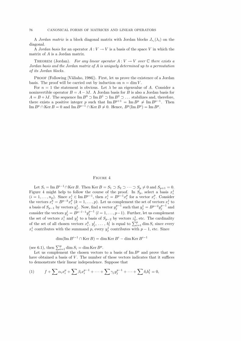
76 CANONICAL FORMS OF MATRICES AND LINEAR OPERATORS
A Jordan matrix is a block diagonal matrix with Jordan blocks Jri(λi) on thediagonal.
A Jordan basis for an operator A : V → V is a basis of the space V in which thematrix of A is a Jordan matrix.
Theorem (Jordan). For any linear operator A : V → V over C there exists aJordan basis and the Jordan matrix of A is uniquely determined up to a permutationof its Jordan blocks.
Proof (Following [Valiaho, 1986]). First, let us prove the existence of a Jordanbasis. The proof will be carried out by induction on n = dimV .
For n = 1 the statement is obvious. Let λ be an eigenvalue of A. Consider anoninvertible operator B = A−λI. A Jordan basis for B is also a Jordan basis forA = B+λI. The sequence ImB0 ⊃ ImB1 ⊃ ImB2 ⊃ . . . stabilizes and, therefore,there exists a positive integer p such that ImBp+1 = ImBp 6= ImBp−1. ThenImBp ∩KerB = 0 and ImBp−1 ∩KerB 6= 0. Hence, Bp(ImBp) = ImBp.
Figure 4
Let Si = ImBi−1∩KerB. Then KerB = S1 ⊃ S2 ⊃ · · · ⊃ Sp 6= 0 and Sp+1 = 0.Figure 4 might help to follow the course of the proof. In Sp, select a basis x1
i
(i = 1, . . . , np). Since x1i ∈ ImBp−1, then x1
i = Bp−1xpi for a vector xpi . Considerthe vectors xki = Bp−kxpi (k = 1, . . . , p). Let us complement the set of vectors x1
i toa basis of Sp−1 by vectors y1
j . Now, find a vector yp−1j such that y1
j = Bp−2yp−1j and
consider the vectors ylj = Bp−l−1yp−1j (l = 1, . . . , p−1). Further, let us complement
the set of vectors x1i and y1
j to a basis of Sp−2 by vectors z1k, etc. The cardinality
of the set of all chosen vectors xki , ylj , . . . , b1t is equal to∑pi=1 dimSi since every
x1i contributes with the summand p, every y1
j contributes with p− 1, etc. Since
dim(ImBi−1 ∩KerB) = dim KerBi − dim KerBi−1
(see 6.1), then∑pi=1 dimSi = dim KerBp.
Let us complement the chosen vectors to a basis of ImBp and prove that wehave obtained a basis of V . The number of these vectors indicates that it sufficesto demonstrate their linear independence. Suppose that
(1) f +∑
αixpi +
∑βix
p−1i + · · ·+
∑γjy
p−1j + · · ·+
∑δtb
1t = 0,
12. THE JORDAN CANONICAL (NORMAL) FORM 77
where f ∈ ImBp. Applying the operator Bp to (1) we get Bp(f) = 0; hence,f = 0 since Bp(ImBp) = ImBp. Applying now the operator Bp−1 to (1) we get∑αix
1i = 0 which means that all αi are zero. Application of the operator Bp−2 to
(1) gives∑βix
1i +
∑γjy
1j = 0, which means that all βi and γj are zero, etc.
By the inductive hypothesis we can select a Jordan basis for B in the spaceImBp 6= V ; complementing this basis by the chosen vectors, we get a Jordan basisof V .
To prove the uniqueness of the Jordan form it suffices to verify that the numberof Jordan blocks of B corresponding to eigenvalue 0 is uniquely defined. To theseblocks we can associate the diagram plotted in Figure 4 and, therefore, the numberof blocks of size k × k is equal to
dimSk − dimSk+1
= (dim KerBk − dim KerBk−1)− (dim KerBk+1 − dim KerBk)
= 2 dim KerBk − dim KerBk−1 − dim KerBk+1
= rankBk−1 − 2 rankBk + rankBk+1;
which is invariantly defined. ¤12.3. The Jordan normal form is convenient to use when we raise a matrix to
some power. Indeed, if A = P−1JP then An = P−1JnP . To raise a Jordan blockJr(λ) = λI +N to a power we can use the Newton binomial formula
(λI +N)n =n∑
k=0
(n
k
)λkNn−k.
The formula holds since IN = NI. The only nonzero elements of Nm are the1’s in the positions (1,m + 1), (2,m + 2), . . . , (r −m, r), where r is the order ofN . If m ≥ r then Nm = 0.
12.4. Jordan bases always exist over an algebraically closed field only; over Ra Jordan basis does not always exist. However, over R there is also a Jordan formwhich is a realification of the Jordan form over C. Let us explain how it looks.First, observe that the part of a Jordan basis corresponding to real eigenvalues ofA is constructed over R along the same lines as over C. Therefore, only the case ofnonreal eigenvalues is of interest.
Let AC be the complexification of a real operator A (cf. 10.1).
12.4.1. Theorem. There is a one-to-one correspondence between the Jordanblocks of AC corresponding to eigenvalues λ and λ.
Proof. Let B = P + iQ, where P and Q are real operators. If x and y arereal vectors then the equations (P + iQ)(x + iy) = 0 and (P − iQ)(x − iy) =0 are equivalent, i.e., the equations Bz = 0 and Bz = 0 are equivalent. Since(A − λI)n = (A− λI)n, the map z 7→ z determines a one-to-one correspondencebetween Ker(A−λI)n and Ker(A−λI)n. The dimensions of these spaces determinethe number and the sizes of the Jordan blocks. ¤
Let J∗n(λ) be the 2n × 2n matrix obtained from the Jordan block Jn(λ) by
replacing each of its elements a+ ib by the matrix(a b−b a
).
78 CANONICAL FORMS OF MATRICES AND LINEAR OPERATORS
12.4.2. Theorem. For an operator A over R there exists a basis with respectto which its matrix is of block diagonal form with blocks Jm1(t1), . . . , Jmk(tk) forreal eigenvalues ti and blocks J∗n1
(λ1), . . . , J∗ns(λs) for nonreal eigenvalues λi andλi.
Proof. If λ is an eigenvalue of A then by Theorem 12.4.1 λ is also an eigenvalueof A and to every Jordan block Jn(λ) of A there corresponds the Jordan block Jn(λ).Besides, if e1, . . . , en is the Jordan basis for Jn(λ) then e1, . . . , en is the Jordan basisfor Jn(λ). Therefore, the real vectors x1, y1, . . . , xn, yn, where ek = xk + iyk, arelinearly independent. In the basis x1, y1, . . . , xn, yn the matrix of the restriction ofA to Span(x1, y1, . . . , xn, yn) is of the form J∗n(λ). ¤
12.5. The Jordan decomposition shows that any linear operator A over C canbe represented in the form A = As+An, where As is a semisimple (diagonalizable)operator and An is a nilpotent operator such that AsAn = AnAs.
12.5.1. Theorem. The operators As and An are uniquely defined; moreover,As = S(A) and An = N(A), where S and N are certain polynomials.
Proof. First, consider one Jordan block A = λI + Nk of size k × k. LetS(t) =
∑mi=1 sit
i. Then
S(A) =m∑
i=1
si
i∑
j=0
(i
j
)λjN i−j
k .
The coefficient of Npk is equal to
∑
i
si
(i
i− p)λi−p =
1p!S(p)(λ),
where S(p) is the pth derivative of S. Therefore, we have to select a polynomial Sso that S(λ) = λ and S(1)(λ) = · · · = S(k−1)(λ) = 0, where k is the order of theJordan block. If λ1, . . . , λn are distinct eigenvalues of A and k1, . . . , kn are the sizesof the maximal Jordan blocks corresponding to them, then S should take value λiat λi and have at λi zero derivatives from order 1 to order ki − 1 inclusive. Sucha polynomial can always be constructed (see Appendix 3). It is also clear that ifAs = S(A) then An = A− S(A), i.e., N(A) = A− S(A).
Now, let us prove the uniqueness of the decomposition. Let As+An = A = A′s+A′n, where AsAn = AnAs and A′sA
′n = A′nA
′s. If AX = XA then S(A)X = XS(A)
and N(A)X = XN(A). Therefore, AsA′s = A′sAs and AnA′n = A′nAn. The opera-
tor B = A′s −As = An −A′n is a difference of commuting diagonalizable operatorsand, therefore, is diagonalizable itself, cf. Problem 39.6 b). On the other hand,the operator B is the difference of commuting nilpotent operators and therefore, isnilpotent itself, cf. Problem 39.6 a). A diagonalizable nilpotent operator is equalto zero. ¤
The additive Jordan decomposition A = As +An enables us to get for an invert-ible operator A a multiplicative Jordan decomposition A = AsAu, where Au is aunipotent operator, i.e., the sum of the identity operator and a nilpotent one.
13. THE MINIMAL POLYNOMIAL AND THE CHARACTERISTIC POLYNOMIAL 79
12.5.2. Theorem. Let A be an invertible operator over C. Then A can berepresented in the form A = AsAu = AuAs, where As is a semisimple operator andAu is a unipotent operator. Such a representation is unique.
Proof. If A is invertible then so is As. Then A = As + An = AsAu whereAu = A−1
s (As +An) = I +A−1s An. Since A−1
s and An commute, then A−1s An is a
nilpotent operator which commutes with As.Now, let us prove the uniqueness. If A = AsAu = AuAs and Au = I +N , where
N is a nilpotent operator, then A = As(I + N) = As + AsN , where AsN is anilpotent operator commuting with A. Such an operator AsN = An is unique. ¤
Problems
12.1. Prove that A and AT are similar matrices.12.2. Let σ(i), where i = 1, . . . , n, be an arbitrary permutation and P =
∥∥pij∥∥n
1,
where pij = δiσ(j). Prove that the matrix P−1AP is obtained from A by thepermutation σ of the rows and the same permutation of the columns of A.
Remark. The matrix P is called the permutation matrix corresponding to σ.12.3. Let the number of distinct eigenvalues of a matrix A be equal to m, where
m > 1. Let bij = tr(Ai+j). Prove that |bij |m−10 6= 0 and |bij |m0 = 0.
12.4. Prove that rankA = rankA2 if and only if limλ→0
(A+ λI)−1A exists.
13. The minimal polynomial and the characteristic polynomial
13.1. Let p(t) =∑nk=0 akt
k be an nth degree polynomial. For any square matrixA we can consider the matrix p(A) =
∑nk=0 akA
k. The polynomial p(t) is called anannihilating polynomial of A if p(A) = 0. (The zero on the right-hand side is thezero matrix.)
If A is an order n matrix, then the matrices I, A, . . . , An2
are linearly dependentsince the dimension of the space of matrices of order n is equal to n2. Therefore,for any matrix of order n there exists an annihilating polynomial whose degree doesnot exceed n2. The annihilating polynomial of A of the minimal degree and withcoefficient of the highest term equal to 1 is called the minimal polynomial of A.
Let us prove that the minimal polynomial is well defined. Indeed, if p1(A) =Am + · · · = 0 and p2(A) = Am + · · · = 0, then the polynomial p1 − p2 annihilatesA and its degree is smaller than m. Hence, p1 − p2 = 0.
It is easy to verify that if B = X−1AX then Bn = X−1AnX and, therefore,p(B) = X−1p(A)X; thus, the minimal polynomial of an operator , not only of amatrix, is well defined.
13.1.1. Theorem. Any annihilating polynomial of a matrix A is divisible byits minimal polynomial.
Proof. Let p be the minimal polynomial of A and q an annihilating polynomial.Dividing q by p with a remainder we get q = pf + r, where deg r < deg p, andr(A) = q(A) − p(A)f(A) = 0, and so r is an annihilating polynomial. Hence,r = 0. ¤
13.1.2. An annihilating polynomial of a vector v ∈ V (with respect to an op-erator A : V → V ) is a polynomial p such that p(A)v = 0. The annihilatingpolynomial of v of minimal degree and with coefficient of the highest term equal to
80 CANONICAL FORMS OF MATRICES AND LINEAR OPERATORS
1 is called the minimal polynomial of v. Similarly to the proof of Theorem 13.1.1,we can demonstrate that the minimal polynomial of A is divisible by the minimalpolynomial of a vector.
Theorem. For any operator A : V → V there exists a vector whose minimalpolynomial (with respect to A) coincides with the minimal polynomial of the oper-ator A.
Proof. Any ideal I in the ring of polynomials in one indeterminate is generatedby a polynomial f of minimal degree. Indeed, if g ∈ I and f ∈ I is a polynomial ofminimal degree, then g = fh+ r, hence, r ∈ I since fh ∈ I.
For any vector v ∈ V consider the ideal Iv = p|p(A)v = 0; this ideal isgenerated by a polynomial pv with leading coefficient 1. If pA is the minimalpolynomial of A, then pA ∈ Iv and, therefore, pA is divisible by pv. Hence, whenv runs over the whole of V we get only a finite number of polynomials pv. Letthese be p1, . . . , pk. The space V is contained in the union of its subspacesVi = x ∈ V | pi(A)x = 0 (i = 1, . . . , k) and, therefore, V = Vi for a certain i.Then pi(A)V = 0; in other words pi is divisible by pA and, therefore, pi = pA. ¤
13.2. Simple considerations show that the degree of the minimal polynomial ofa matrix A of order n does not exceed n2. It turns out that the degree of theminimal polynomial does not actually exceed n, since the characteristic polynomialof A is an annihilating polynomial.
Theorem (Cayley-Hamilton). Let p(t) = |tI −A|. Then p(A) = 0.
Proof. For the Jordan form of the operator the proof is obvious because (t−λ)n
is an annihilating polynomial of Jn(λ). Let us, however, give a proof which doesnot make use of the Jordan theorem.
We may assume that A is a matrix (in a basis) of an operator over C. Let uscarry out the proof by induction on the order n of A. For n = 1 the statement isobvious.
Let λ be an eigenvalue of A and e1 the corresponding eigenvector. Let us com-plement e1 to a basis e1, . . . , en. In the basis e1, . . . , en the matrix A is of the
form(λ ∗0 A1
), where A1 is the matrix of the operator in the quotient space
V/ Span(e1). Therefore, p(t) = (t − λ)|tI − A1| = (t − λ)p1(t). By inductivehypothesis p1(A1) = 0 in V/ Span(e1), i.e., p1(A1)V ⊂ Span(e1). It remains toobserve that (λI −A)e1 = 0. ¤
Remark. Making use of the Jordan normal form it is easy to verify that theminimal polynomial of A is equal to
∏i(t − λi)ni , where the product runs over
all distinct eigenvalues λi of A and ni is the order of the maximal Jordan blockcorresponding to λi. In particular, the matrix A is diagonalizable if and only if theminimal polynomial has no multiple roots and all its roots belong to the groundfield.
13.3. By the Cayley-Hamilton theorem the characteristic polynomial of a matrixof order n coincides with its minimal polynomial if and only if the degree of theminimal polynomial is equal to n. The minimal polynomial of a matrix A is theminimal polynomial for a certain vector v (cf. Theorem 13.1.2). Therefore, thecharacteristic polynomial coincides with the minimal polynomial if and only if fora certain vector v the vectors v, Av, . . . , An−1v are linearly independent.
13. THE MINIMAL POLYNOMIAL AND THE CHARACTERISTIC POLYNOMIAL 81
Theorem ([Farahat, Lederman, 1958]). The characteristic polynomial of a ma-trix A of order n coincides with its minimal polynomial if and only if for any vector(x1, . . . , xn) there exist columns P and Q of length n such that xk = QTAkP .
Proof. First, suppose that the degree of the minimal polynomial of A is equalto n. Then there exists a column P such that the columns P , AP , . . . , An−1Pare linearly independent, i.e., the matrix K formed by these columns is invertible.Any vector X = (x1, . . . , xn) can be represented in the form X = (XK−1)K =(QTP, . . . , QTAn−1P ), where QT = XK−1.
Now, suppose that for any vector (x1, . . . , xn) there exist columns P and Q suchthat xk = QTAkP . Then there exist columns P1, . . . , Pn, Q1, . . . , Qn such that thematrix
B =
QT1 P1 . . . QT1 A
n−1P1
... · · · ...QTnPn . . . QTnA
n−1Pn
is invertible. The matrices I, A, . . . , An−1 are linearly independent because oth-erwise the columns of B would be linearly dependent. ¤
13.4. The Cayley-Hamilton theorem has several generalizations. We will confineourselves to one of them.
13.4.1. Theorem ([Greenberg, 1984]). Let pA(t) be the characteristic polyno-mial of a matrix A, and let a matrix X commute with A. Then pA(X) = M(A−X),where M is a matrix that commutes with A and X.
Proof. Since B · adjB = |B| · I (see 2.4),
pA(λ) · I = [adj(λI −A)](λI −A) = (n−1∑
k=0
Akλk)(λI −A) =
n∑
k=0
λkA′k.
All matrices A′k are diagonal, since so is pA(λ)I. Hence, pA(X) =∑nk=0X
kA′k. If Xcommutes with A and Ak, then pA(X) = (
∑n−1k=0 AkX
k)(X −A). But the matricesAk can be expressed as polynomials of A (see Problem 2.11) and, therefore, if Xcommutes with A then X commutes with Ak. ¤
Problems
13.1. Let A be a matrix of order n and
f1(A) = A− (trA)I, fk+1(A) = fk(A)A− 1k + 1
tr(fk(A)A)I.
Prove that fn(A) = 0.13.2. Let A and B be matrices of order n. Prove that if trAm = trBm for
m = 1, . . . , n then the eigenvalues of A and B coincide.13.3. Let a matrix A be invertible and let its minimal polynomial p(λ) coincide
with its characteristic polynomial. Prove that the minimal polynomial of A−1 isequal to p(0)−1λnp(λ−1).
13.4. Let the minimal polynomial of a matrix A be equal to∏
(x− λi)ni . Prove
that the minimal polynomial of(A I0 A
)is equal to
∏(x− λi)ni+1.
82 CANONICAL FORMS OF MATRICES AND LINEAR OPERATORS
14. The Frobenius canonical form
14.1. The Jordan form is just one of several canonical forms of matrices of linearoperators. An example of another canonical form is the cyclic form also known asthe Frobenius canonical form.
A Frobenius or cyclic block is a matrix of the form
0 0 0 . . . 0 −a0
1 0 0 . . . 0 −a1
0 1 0 . . . 0 −a2...
......
. . . . . ....
0 0 0 . . . 1 −an−1
.
If A : V n → V n and Ae1 = e2, . . . , Aen−1 = en then the matrix of the operator Awith respect to e1, . . . , en is a cyclic block.
Theorem. For any linear operator A : V → V (over C or R) there exists abasis in which the matrix of A is of block diagonal form with cyclic diagonal blocks.
Proof (Following [Jacob, 1973]). We apply induction on dimV . If the degreeof the minimal polynomial of A is equal to k, then there exists a vector y ∈ V thedegree of whose minimal polynomial is also equal to k (see Theorem 13.1.2). Letyi = Ai−1y. Let us complement the basis y1, . . . , yk of W = Span(y1, . . . , yk) toa basis of V and consider W ∗1 = Span(y∗k, A
∗y∗k, . . . , A∗k−1y∗k). Let us prove that
V = W ⊕W ∗⊥1 is an A-invariant decomposition of V .The degree of the minimal polynomial of A∗ is also equal to k and, therefore,
W ∗1 is invariant with respect to A∗; hence, (W ∗1 )⊥ is invariant with respect to A.It remains to demonstrate that W ∗1 ∩ W⊥ = 0 and dimW ∗1 = k. Suppose thata0y∗k + · · · + asA
∗sy∗k ∈ W⊥ for 0 ≤ s ≤ k − 1 and as 6= 0. Then A∗k−s−1(a0y∗k +
· · ·+ asA∗sy∗k) ∈W⊥; hence,
0 = 〈a0A∗k−s−1y∗k + · · ·+ asA
k−1y∗k, y〉= a0〈y∗k, Ak−s−1y〉+ · · ·+ as〈y∗k, Ak−1y〉= a0〈y∗k, yk−s〉+ · · ·+ as〈y∗k, yk〉 = as.
Contradiction.The matrix of the restriction of A to W in the basis y1, . . . , yk is a cyclic block.
The restriction of A toW ∗⊥1 can be represented in the required form by the inductivehypothesis. ¤
Remark. In the process of the proof we have found a basis in which the matrix ofA is of block diagonal form with cyclic blocks on the diagonal whose characteristicpolynomials are p1, p2, . . . , pk, where p1 is the minimal polynomial for A, p2 theminimal polynomial of the restriction of A to a subspace, and, therefore, p2 is adivisor of p1. Similarly, pi+1 is a divisor of pi.
15. HOW TO REDUCE THE DIAGONAL TO A CONVENIENT FORM 83
14.2. Let us prove that the characteristic polynomial of the cyclic block
A =
0 0 . . . 0 0 0 −a0
1 0 . . . 0 0 0 −a1
0 1 . . . 0 0 0 −a2...
.... . .
......
0 0 . . . 1 0 0 −an−3
0 0 . . . 0 1 0 −an−2
0 0 . . . 0 0 1 −an−1
is equal to λn +∑n−1k=0 akλk. Indeed, since Ae1 = e2, . . . , Aen−1 = en, and
Aen = −∑n−1k=0 akek+1, it follows that
(An +
n−1∑
k=0
akAk
)e1 = 0.
Taking into account that ei = Ai−1e1 we see that λn+∑n−1k=0 akλ
k is an annihilatingpolynomial of A. It remains to notice that the vectors e1, Ae1, . . . , An−1e1 arelinearly independent and, therefore, the degree of the minimal polynomial of A isno less than n.
As a by product we have proved that the characteristic polynomial of a cyclicblock coincides with its minimal polynomial.
Problems
14.1. The matrix of an operator A is block diagonal and consists of two cyclicblocks with relatively prime characteristic polynomials, p and q. Prove that it ispossible to select a basis so that the matrix becomes one cyclic block.
14.2. Let A be a Jordan block, i.e., there exists a basis e1, . . . , en such thatAe1 = λe1 and Aek = ek−1 + λek for k = 2, . . . , n. Prove that there exists a vectorv such that the vectors v, Av, . . . , An−1v constitute a basis (then the matrix ofthe operator A with respect to the basis v,Av, . . . , An−1v is a cyclic block).
14.3. For a cyclic block A indicate a symmetric matrix S such that A = SATS−1.
15. How to reduce the diagonal to a convenient form
15.1. The transformation A 7→ XAX−1 preserves the trace and, therefore, thediagonal elements of the matrix XAX−1 cannot be made completely arbitrary. Wecan, however, reduce the diagonal of A to a, sometimes, more convenient form;for example, a matrix A 6= λI is similar to a matrix whose diagonal elements are(0, . . . , 0, trA); any matrix is similar to a matrix all diagonal elements of which areequal.
Theorem ([Gibson, 1975]). Let A 6= λI. Then A is similar to a matrix with thediagonal (0, . . . , 0, trA).
Proof. The diagonal of a cyclic block is of the needed form. Therefore, thestatement is true for any matrix whose characteristic and minimal polynomialscoincide (cf. 14.1).
84 CANONICAL FORMS OF MATRICES AND LINEAR OPERATORS
For a matrix of order 2 the characteristic polynomial does not coincide with theminimal one only for matrices of the form λI. Let now A be a matrix of order 3such that A 6= λI and the characteristic polynomial of A does not coincide with itsminimal polynomial. Then the minimal polynomial of A is of the form (x−λ)(x−µ)whereas the characteristic polynomial is (x− λ)2(x− µ) and the case λ = µ is not
excluded. Therefore, the matrix A is similar to the matrix C =
0 a 01 b 00 0 λ
and
the characteristic polynomial of(
0 a1 b
)is divisible by x−λ, i.e., λ2− bλ− a = 0.
If b = λ = 0, then the theorem holds.If b = λ 6= 0, then b2 − b2 − a = 0, i.e., a = 0. In this case
0 0 01 b 00 0 b
b b b−1 0 0b 0 b
=
0 0 00 b bb2 0 b2
=
b b b−1 0 0b 0 b
0 −b −b−b 0 −bb b 2b
,
and det
b b b−1 0 0b 0 b
6= 0; therefore, A is similar to
0 −b −b−b 0 −bb b 2b
.
Let, finally, b 6= λ. Then for the matrix D = diag(b, λ) the theorem is true and,
therefore, there exists a matrix P such that PDP−1 =(
0 ∗∗ ∗
). The matrix
(1 00 P
)C
(1 00 P−1
)=
(1 00 P
)(0 ∗∗ D
)(1 00 P−1
)=
(0 ∗∗ PDP−1
)
is of the required form.Now, suppose our theorem holds for matrices of order m, where m ≥ 3. A matrix
A of order m+ 1 is of the form(A1 ∗∗ ∗
), where A1 is a matrix of order m. Since
A 6= λI, we can assume that A1 6= λI (otherwise we perform a permutation of rowsand columns, cf. Problem 12.2). By the inductive hypothesis there exists a matrixP such that the diagonal of the matrix PA1P
−1 is of the form (0, 0, . . . , 0, α) and,therefore, the diagonal of the matrix
X =(P 00 1
)(A1 ∗∗ ∗
)(P−1 0
0 1
)=
(PA1P
−1 ∗∗ ∗
)
is of the form (0, . . . , 0, α, β). If α = 0 we are done.
Let α 6= 0. Then X =(
0 ∗∗ C1
), where the diagonal of the matrix C1 of order
m is of the form (0, 0, . . . , α, β) and, therefore, C1 6= λI. Hence, there exists amatrix Q such that the diagonal of QCQ−1 is of the form (0, . . . , 0, x). Therefore,
the diagonal of(
1 00 Q
)(0 ∗∗ C1
)(1 00 Q−1
)is of the required form. ¤
Remark. The proof holds for a field of any characteristic.
15. HOW TO REDUCE THE DIAGONAL TO A CONVENIENT FORM 85
15.2. Theorem. Let A be an arbitrary complex matrix. Then there exists aunitary matrix U such that the diagonal elements of UAU−1 are equal.
Proof. On the set of unitary matrices, consider a function f whose value at Uis equal to the maximal absolute value of the difference of the diagonal elementsof UAU−1. This function is continuous and is defined on a compact set and,therefore, it attains its minimum on this compact set. Therefore, to prove thetheorem it suffices to show that with the help of the transformation A 7→ UAU−1
one can always diminish the maximal absolute value of the difference of the diagonalelements unless it is already equal to zero.
Let us begin with matrices of size 2 × 2. Let u = cosαeiϕ, v = sinαeiψ. Thenin the (1, 1) position of the matrix
(u v−v u
)(a1 bc a2
)(u −vv u
)
there stands
a1 cos2 α+ a2 sin2 α+ (beiβ + ce−iβ) cosα sinα, where β = ϕ− ψ.When β varies from 0 to 2π the points beiβ + ce−iβ form an ellipse (or an interval)centered at 0 ∈ C. Indeed, the points eiβ belong to the unit circle and the map z 7→bz + cz determines a (possibly singular) R-linear transformation of C. Therefore,the number
p = (beiβ + ce−iβ)/(a1 − a2)
is real for a certain β. Hence, t = cos2 α+ p sinα cosα is also real and
a1 cos2 α+ a2 sin2 α+ (beiβ + ce−iβ) cosα sinα = ta1 + (1− t)a2.
As α varies from 0 to π2 , the variable t varies from 1 to 0. In particular, t takes
the value 12 . In this case the both diagonal elements of the transformed matrix are
equal to 12 (a11 + a22).
Let us treat matrices of size n × n, where n ≥ 3, as follows. Select a pair ofdiagonal elements the absolute value of whose difference is maximal (there could beseveral such pairs). With the help of a permutation matrix this pair can be placed inthe positions (1, 1) and (2, 2) thanks to Problem 12.2. For the matrix A′ =
∥∥aij∥∥2
1
there exists a unitary matrix U such that the diagonal elements of UA′U−1 areequal to 1
2 (a11 + a22). It is also clear that the transformation A 7→ U1AU−11 , where
U1 is the unitary matrix(U 00 I
), preserves the diagonal elements a33, . . . , ann .
Thus, we have managed to replace two fartherest apart diagonal elements a11 anda22 by their arithmetic mean. We do not increase in this way the maximal distancebetween points nor did we create new pairs the distance between which is equal to|a11 − a22| since
|x− a11 + a22
2| ≤ |x− a11|
2+|x− a22|
2.
After a finite number of such steps we get rid of all pairs of diagonal elements thedistance between which is equal to |a11 − a22|. ¤
Remark. If A is a real matrix, then we can assume that u = cosα and v = sinα.The number p is real in such a case. Therefore, if A is real then U can be consideredto be an orthogonal matrix.
86 CANONICAL FORMS OF MATRICES AND LINEAR OPERATORS
15.3. Theorem ([Marcus, Purves, 1959]). Any nonzero square matrix A issimilar to a matrix all diagonal elements of which are nonzero.
Proof. Any matrix A of order n is similar to a matrix all whose diagonalelements are equal to 1
n trA (see 15.2), and, therefore, it suffices to consider thecase when trA = 0. We can assume that A is a Jordan block.
First, let us consider a matrix A =∥∥aij
∥∥n1
such that aij = δ1iδ2j . If U =∥∥uij
∥∥is a unitary matrix then UAU−1 = UAU∗ = B, where bii = ui1ui2. We can selectU so that all elements ui1, ui2 are nonzero.
The rest of the proof will be carried out by induction on n; for n = 2 thestatement is proved.
Recall that we assume that A is in the Jordan form. First, suppose that A is a
diagonal matrix and a11 6= 0. Then A =(a11 00 Λ
), where Λ is a nonzero diagonal
matrix. Let U be a matrix such that all elements of UΛU−1 are nonzero. Then thediagonal elements of the matrix
(1 00 U
) (a11 00 Λ
)(1 00 U−1
)=
(a11 00 UΛU−1
)
are nonzero.Now, suppose that a matrix A is not diagonal. We can assume that a12 = 1 and
the matrix C obtained from A by crossing out the first row and the first columnis a nonzero matrix. Let U be a matrix such that all diagonal elements of UCU−1
are nonzero. Consider the matrix
D =(
1 00 U
)A
(1 00 U−1
)=
(a11 ∗0 UCU−1
).
The only zero diagonal element of D could be a11. If a11 = 0 then for(
0 ∗0 d22
)
select a matrix V such that the diagonal elements of V(
0 ∗0 d22
)V −1 are nonzero.
Then the diagonal elements of(V 00 I
)D
(V −1 0
0 I
)are also nonzero. ¤
Problem
15.1. Prove that for any nonzero square matrix A there exists a matrix X suchthat the matrices X and A+X have no common eigenvalues.
16. The polar decomposition
16.1. Any complex number z can be represented in the form z = |z|eiϕ. Ananalogue of such a representation is the polar decomposition of a matrix, A = SU ,where S is an Hermitian and U is a unitary matrix.
Theorem. Any square matrix A over R (or C) can be represented in the formA = SU , where S is a symmetric (Hermitian) nonnegative definite matrix and U isan orthogonal (unitary) matrix. If A is invertible such a representation is unique.
Proof. If A = SU , where S is an Hermitian nonnegative definite matrix and Uis a unitary matrix, then AA∗ = SUU∗S = S2. To find S, let us do the following.
17. FACTORIZATIONS OF MATRICES 87
The Hermitian matrix AA∗ has an orthonormal eigenbasis and AA∗ei = λ2i ei,
where λi ≥ 0 . Set Sei = λiei. The Hermitian nonnegative definite matrix S isuniquely determined by A. Indeed, let e′1, . . . , e
′n be an orthonormal eigenbasis for
S and Se′i = λ′ie′i, where λ′i ≥ 0 . Then (λ′i)
2e′i = S2e′i = AA∗e′i and this equationuniquely determines λ′i.
Let v1, . . . , vn be an orthonormal basis of eigenvectors of the Hermitian operatorA∗A and A∗Avi) = µ2
i vi, where µi ≥ 0. Since (Avi, Avj) = (vi, A∗Avj) = µ2i (vi, vj),
we see that the vectors Av1, . . . , Avn are pairwise orthogonal and |Avi| = µi. There-fore, there exists an orthonormal basis w1, . . . , wn such that Avi = µiwi. SetUvi = wi and Swi = µiwi. Then SUvi = Swi = µiwi = Avi, i.e., A = SU .
In the decomposition A = SU the matrix S is uniquely defined. If S is invertiblethen U = S−1A is also uniquely defined. ¤
Remark. We can similarly construct a decomposition A = U1S1, where S1
is a symmetric (Hermitian) nonnegative definite matrix and U1 is an orthogonal(unitary) matrix. Here S1 = S if and only if AA∗ = A∗A, i.e., the matrix A isnormal.
16.2.1. Theorem. Any matrix A can be represented in the form A = UDW ,where U and W are unitary matrices and D is a diagonal matrix.
Proof. Let A = SV , where S is Hermitian and V unitary. For S there exists aunitary matrix U such that S = UDU∗, where D is a diagonal matrix. The matrixW = U∗V is unitary and A = SV = UDW . ¤
16.2.2. Theorem. If A = S1U1 = U2S2 are the polar decompositions of aninvertible matrix A, then U1 = U2.
Proof. Let A = UDW , where D = diag(d1, . . . , dn) is a diagonal matrix, andU and W are unitary matrices. Consider the matrix D+ = diag(|d1|, . . . , |dn|); thenDD+ = D+D and, therefore,
A = (UD+U∗)(UD−1
+ DW ) = (UD−1+ DW )(W ∗D+W ).
The matrices UD+U∗ and W ∗D+W are positive definite and D−1
+ D is unitary.The uniqueness of the polar decomposition of an invertible matrix implies thatS1 = UD+U
∗, S2 = W ∗D+W and U1 = UD−1+ DW = U2. ¤
Problems
16.1. Prove that any linear transformation of Rn is the composition of an or-thogonal transformation and a dilation along perpendicular directions (with distinctcoefficients).
16.2. Let A : Rn → Rn be a contraction operator, i.e., |Ax| ≤ |x|. The space Rncan be considered as a subspace of R2n. Prove that A is the restriction to Rn ofthe composition of an orthogonal transformation of R2n and the projection on Rn.
17. Factorizations of matrices
17.1. The Schur decomposition.
88 CANONICAL FORMS OF MATRICES AND LINEAR OPERATORS
Theorem (Schur). Any square matrix A over C can be represented in the formA = UTU∗, where U is a unitary and T a triangular matrix; moreover, A is normalif and only if T is a diagonal matrix.
Proof. Let us prove by induction on the order of A. Let x be an eigenvector ofA, i.e., Ax = λx. We may assume that |x| = 1. Let W be a unitary matrix whosefirst column is made of the coordinates of x (to construct such a matrix it sufficesto complement x to an orthonormal basis). Then
W ∗AW =
λ ∗ ∗ ∗0...0
A1
.
By the inductive hypothesis there exists a unitary matrix V such that V ∗A1V is a
triangular matrix. Then U =(
1 00 V
)is the desired matrix.
It is easy to verify that the equations T ∗T = TT ∗ and A∗A = AA∗ are equivalent.It remains to prove that a triangular normal matrix is a diagonal matrix. Let
T =
t11 t12 . . . t1n0 t21 . . . t1n...
. . . . . ....
0 0 . . . tnn
.
Then (TT ∗)11 = |t11|2 + |t12|2 + · · · + |t1n|2 and (T ∗T )11 = |t11|2. Therefore, theidentity TT ∗ = T ∗T implies that t12 = · · · = t1n = 0.
Now, strike out the first row and the first column in T and repeat the argu-ments. ¤
17.2. The Lanczos decomposition.
Theorem ([Lanczos, 1958]). Any real m × n-matrix A of rank p > 0 can berepresented in the form A = XΛY T , where X and Y are matrices of size m × pand n× p with orthonormal columns and Λ is a diagonal matrix of size p× p.
Proof (Following [Schwert, 1960]). The rank of ATA is equal to the rankof A; see Problem 8.3. Let U be an orthogonal matrix such that UTATAU =diag(µ1, . . . , µp, 0, . . . , 0), where µi > 0. Further, let y1, . . . , yp be the first p columnsof U and Y the matrix formed by these columns. The columns xi = λ−1
i Ayi, whereλi =
õi, constitute an orthonormal system since (Ayi, Ayj) = (yi, ATAyj) =
λ2j (yi, yj). It is also clear that AY = (λ1x1, . . . , λpxp) = XΛ, where X is a ma-
trix constituted from x1, . . . , xp, Λ = diag(λ1, . . . , λp). Now, let us prove thatA = XΛY T . For this let us again consider the matrix U = (Y, Y0). SinceKerATA = KerA and (ATA)Y0 = 0, it follows that AY0 = 0. Hence, AU = (XΛ, 0)and, therefore, A = (XΛ, 0)UT = XΛY T . ¤
Remark. Since AU = (XΛ, 0), then UTAT =(
ΛXT
0
). Multiplying this
equality by U , we get AT = Y ΛXT . Hence, ATX = Y ΛXTX = Y Λ, sinceXTX = Ip. Therefore, (XTA)(ATX) = (ΛY T )(Y Λ) = Λ2, since Y TY = Ip. Thus,the columns of X are eigenvectors of AAT .
18. THE SMITH NORMAL FORM. ELEMENTARY FACTORS OF MATRICES 89
17.3. Theorem. Any square matrix A can be represented in the form A = ST ,where S and T are symmetric matrices, and if A is real, then S and T can also beconsidered to be real matrices.
Proof. First, observe that if A = ST , where S and T are symmetric matrices,then A = ST = S(TS)S−1 = SATS−1, where S is a symmetric matrix. The otherway around, if A = SATS−1, where S is a symmetric matrix, then A = ST , whereT = ATS−1 is a symmetric matrix, since (ATS−1)T = S−1A = S−1SATS−1 =ATS−1.
If A is a cyclic block then there exists a symmetric matrix S such that A =SATS−1 (Problem 14.3). For any A there exists a matrix P such that B = P−1APis in Frobenius form. For B there exists a symmetric matrix S such that B =SBTS−1. Hence, A = PBP−1 = PSBTS−1P−1 = S1AS
−11 , where S1 = PSPT is
a symmetric matrix. ¤To prove the theorem we could have made use of the Jordan form as well. In
order to do this, it suffices to notice that, for example,
Λ E 00 Λ E0 0 Λ
=
0 0 E0 E 0E 0 0
0 0 Λ′
0 Λ′ EΛ′ E 0
,
where Λ = Λ′ = λ and E = 1 for the real case (or for a real λ) and for the complex
case (i.e., λ = a + bi, b 6= 0) Λ =(a b−b a
), E =
(0 11 0
)and Λ′ =
(b aa −b
).
For a Jordan block of an arbitrary size a similar decomposition also holds.
Problems
17.1 (The Gauss factorization). All minors |aij |p1, p = 1, . . . , n of a matrix A oforder n are nonzero. Prove that A can be represented in the form A = T1T2, whereT1 is a lower triangular and T2 an upper triangular matrix.
17.2 (The Gram factorization). Prove that an invertible matrix X can be repre-sented in the form X = UT , where U is an orthogonal matrix and T is an uppertriangular matrix.
17.3 ([Ramakrishnan, 1972]). Let B = diag(1, ε, . . . , εn−1), where ε = exp( 2πin ),
and C =∥∥cij
∥∥n1, where cij = δi,j−1 (here j − 1 is considered modulo n). Prove
that any n × n-matrix M over C is uniquely representable in the form M =∑n−1k,l=0 aklB
kCl.17.4. Prove that any skew-symmetric matrix A can be represented in the form
A = S1S2 − S2S1, where S1 and S2 are symmetric matrices.
18. The Smith normal form. Elementary factors of matrices
18.1. Let A be a matrix whose elements are integers or polynomials (we mayassume that the elements of A belong to a commutative ring in which the notionof the greatest common divisor is defined). Further, let fk(A) be the greatestcommon divisor of minors of order k of A. The formula for determinant expansionwith respect to a row indicates that fk is divisible by fk−1.
The formula A−1 = (adjA)/detA shows that the elements of A−1 are integers(resp. polynomials) if detA = ±1 (resp. detA is a nonzero number). The other way
90 CANONICAL FORMS OF MATRICES AND LINEAR OPERATORS
around, if the elements of A−1 are integers (resp. polynomials) then detA = ±1(resp. detA is a nonzero number) since detA ·detA−1 = det(AA−1) = 1. MatricesA with detA = ±1 are called unities (of the corresponding matrix ring). Theproduct of unities is, clearly, a unity.
18.1.1. Theorem. If A′ = BAC, where B and C are unity matrices, thenfk(A′) = fk(A) for all admissible k.
Proof. From the Binet-Cauchy formula it follows that fk(A′) is divisible byfk(A). Since A = B−1A′C−1, then fk(A) is divisible by fk(A′). ¤
18.1.2. Theorem (Smith). For any matrix A of size m × n there exist unitymatrices B and C such that BAC = diag(g1, g2, . . . , gp, 0, . . . , 0), where gi+1 isdivisible by gi.
The matrix diag(g1, g2, . . . , gp, 0, . . . , 0) is called the Smith normal form of A.
Proof. The multiplication from the right (left) by the unity matrix∥∥aij
∥∥n1,
where aii = 1 for i 6= p, q and apq = aqp = 1 the other elements being zero,performs a permutation of pth column (row) with the qth one. The multiplicationfrom the right by the unity matrix
∥∥aij∥∥n
1, where aii = 1 (i = 1, . . . , n) and apq = f
(here p and q are fixed distinct numbers), performs addition of the pth columnmultiplied by f to the qth column whereas the multiplication by it from the leftperforms the addition of the qth row multiplied by f to the pth one. It remains toverify that by such operations the matrix A can be reduced to the desired form.
Define the norm of an integer as its absolute value and the norm of a polynomialas its degree. Take a nonzero element a of the given matrix with the least normand place it in the (1, 1) position. Let us divide all elements of the first row by awith a remainder and add the multiples of the first column to the columns 2 to nso that in the first row we get the remainders after division by a.
Let us perform similar operations over columns. If after this in the first rowand the first column there is at least one nonzero element besides a then its normis strictly less than that of a. Let us place this element in the position (1, 1) andrepeat the above operations. The norm of the upper left element strictly diminishesand, therefore, at the end in the first row and in the first column we get just onenonzero element, a11.
Suppose that the matrix obtained has an element aij not divisible by a11. Add tothe first column the column that contains aij and then add to the row that containsaij a multiple of the first row so that the element aij is replaced by the remainderafter division by a11. As a result we get an element whose norm is strictly less thanthat of a11. Let us place it in position (1, 1) and repeat the indicated operations.
At the end we get a matrix of the form(g1 00 A′
), where the elements of A′ are
divisible by g1.Now, we can repeat the above arguments for the matrix A′. ¤
Remark. Clearly, fk(A) = g1g2 . . . gk.
18.2. The elements g1, . . . , gp obtained in the Smith normal form are calledinvariant factors of A. They are expressed in terms of divisors of minors fk(A) asfollows: gk = fk/fk−1 if fk−1 6= 0.
SOLUTIONS 91
Every invariant factor gi can be expanded in a product of powers of primes (resp.powers of irreducible polynomials). Such factors are called elementary divisors ofA. Each factor enters the set of elementary divisors multiplicity counted.
Elementary divisors of real or complex matrix A are elementary divisors of thematrix xI − A. The product of all elementary divisors of a matrix A is equal, upto a sign, to its characteristic polynomial.
Problems
18.1. Compute the invariant factors of a Jordan block and of a cyclic block.18.2. Let A be a matrix of order n, let fn−1 be the greatest common divisor of
the (n − 1)-minors of xI − A. Prove that the minimal polynomial A is equal to|xI −A|fn−1
.
Solutions
11.1. a) The trace of AB − BA is equal to 0 and, therefore, AB − BA cannotbe equal to I.
b) If |A| 6= 0 and AB − BA = A, then A−1AB − A−1BA = I. But tr(B −A−1BA) = 0 and tr I = n.
11.2. Let all elements of B be equal to 1 and Λ = diag(λ1, . . . , λn). ThenA = ΛBΛ−1 and if x is an eigenvector of B then Λx is an eigenvector of A. Thevector (1, . . . , 1) is an eigenvector of B corresponding to the eigenvalue n and the(n− 1)-dimensional subspace x1 + · · ·+ xn = 0 is the eigenspace corresponding toeigenvalue 0.
11.3. If λ is not an eigenvalue of the matrices ±A, then A can be represented asone half times the sum of the invertible matrices A+ λI and A− λI.
11.4. Obviously, the coefficients of the characteristic polynomial depend contin-uously on the elements of the matrix. It remains to prove that the roots of thepolynomial p(x) = xn + a1x
n−1 + · · · + an depend continuously on a1, . . . , an. Itsuffices to carry out the proof for the zero root (for a nonzero root x1 we can con-sider the change of variables y = x − x1). If p(0) = 0 then an = 0. Consider apolynomial q(x) = xn + b1x
n−1 + · · ·+ bn, where |bi− ai| < δ. If x1, . . . , xn are theroots of q, then |x1 . . . xn| = |bn| < δ and, therefore, the absolute value of one ofthe roots of q is less than n
√δ. The δ required can be taken to be equal to εn.
11.5. If the sum of the elements of every row of A is equal to s, then Ae =se, where e is the column (1, 1, . . . , 1)T . Therefore, A−1(Ae) = A−1(se); hence,A−1e = (1/s)e, i.e., the sum of the elements of every row of A−1 is equal to 1/s.
11.6. Let S1 be the first column of S. Equating the first columns of AS and SΛ,where the first column of Λ is of the form (λ, 0, . . . , 0)T , we get AS1 = λS1.
11.7. It is easy to verify that |λI − A| = ∑nk=0 λ
n−k(−1)k∆k(A), where ∆k(A)is the sum of all principal k-minors of A. It follows that
n∑
i=1
|λI −Ai| =n∑
i=1
n−1∑
k=0
λn−k−1(−1)k∆k(Ai).
It remains to notice thatn∑
i=1
∆k(Ai) = (n− k)∆k(A),
92 CANONICAL FORMS OF MATRICES AND LINEAR OPERATORS
since any principal k-minor of A is a principal k-minor for n− k matrices Ai.11.8. Since adj(PXP−1) = P (adjX)P−1, we can assume that A is in the Jordan
normal form. In this case adjA is an upper triangular matrix (by Problem 2.6) andit is easy to compute its diagonal elements.
11.9. Let S =∥∥δi,n−j
∥∥n0. Then AS =
∥∥bij∥∥n
0and SA =
∥∥cij∥∥n
0, where bij =
ai,n−j and cij = an−i,j . Therefore, the central symmetry of Ameans that AS = SA.It is also easy to see that x is a symmetric vector if Sx = x and skew-symmetric ifSx = −x.
Let λ be an eigenvalue of A and Ay = λy, where y 6= 0. Then A(Sy) = S(Ay) =S(λy) = λ(Sy). If Sy = −y we can set x = y. If Sy 6= −y we can set x = y + Syand then Ax = λx and Sx = x.
11.10. SinceAei = an−i+1,ien−i+1 = xn−i+1en−i+1
and Aen−i+1 = xiei, the subspaces Vi = Span(ei, en−i+1) are invariant with respectto A. For i 6= n − i + 1 the matrix of the restriction of A to Vi is of the form
B =(
0 λµ 0
). The eigenvalues of B are equal to ±√λµ. If λµ = 0 and B is
diagonalizable, then B = 0. Therefore, the matrix B is diagonalizable if and onlyif both numbers λ and µ are simultaneously equal or not equal to zero.
Thus, the matrix A is diagonalizable if and only if the both numbers xi andxn−i+1 are simultaneously equal or not equal to 0 for all i.
11.11. a) Suppose the columns x1, . . . , xm correspond to real eigenvalues α1,. . . , αm. Let X = (x1, . . . , xm) and D = diag(α1, . . . , αm). Then AX = XD andsince D is a real matrix, then AXX∗ = XDX∗ = X(XD)∗ = X(AX)∗ = XX∗A∗.If the vectors x1, . . . , xm are linearly independent, then rankXX∗ = rankX = m(see Problem 8.3) and, therefore, for S we can take XX∗.
Now, suppose that AS = SA∗ and S is a nonnegative definite matrix of rank m.Then there exists an invertible matrix P such that S = PNP ∗, where N =(Im 00 0
). Let us multiply both parts of the identity AS = SA∗ by P−1 from
the left and by (P ∗)−1 from the right; we get (P−1AP )N = N(P−1AP )∗. Let
P−1AP = B =(B11 B12
B21 B22
), where B11 is a matrix of order m. Since BN = NB∗,
then(B11 0B21 0
)=
(B∗11 B∗21
0 0
), i.e., B =
(B11 B12
0 B22
), where B11 is an Her-
mitian matrix of order m. The matrix B11 has m linearly independent eigenvectorsz1, . . . , zm with real eigenvalues. Since AP = PB and P is an invertible matrix,then the vectors P
(z10
), . . . , P
(zm0
)are linearly independent and are eigenvectors
of A corresponding to real eigenvalues.b) The proof is largely similar to that of a): in our case AXX∗A∗ = AX(AX)∗ =
XD(XD)∗ = XDD∗X∗ = XX∗.If ASA∗ = S and S = PNP ∗, then P−1APN(P−1AP )∗ = N , i.e.,
(B11B
∗11 B11B
∗21
B21B∗11 B21B
∗21
)=
(Im 00 0
).
Therefore, B21 = 0 and P−1AP = B =(B11 B12
0 B22
), where B11 is unitary.
SOLUTIONS 93
12.1. Let A be a Jordan block of order k. It is easy to verify that in this caseSkA = ATSk, where Sk =
∥∥δi,k+1−j∥∥k
1is an invertible matrix. If A is the direct
sum of Jordan blocks, then we can take the direct sum of the matrices Sk.12.2. The matrix P−1 corresponds to the permutation σ−1 and, therefore, P−1 =∥∥qij∥∥n
1, where qij = δσ(i)j . Let P−1AP =
∥∥bij∥∥n
1. Then bij =
∑s,t δσ(i)sastδtσ(j) =
aσ(i)σ(j).12.3. Let λ1, . . . , λm be distinct eigenvalues of A and pi the multiplicity of the
eigenvalue λi. Then tr(Ak) = p1λk1 + · · ·+ pmλ
km. Therefore,
∥∥bij∥∥m−1
0= p1 . . . pm
∏
i 6=j(λi − λj)2 (See Problem 1.18).
To compute |bij |m0 we can, for example, replace pmλkm with λkm+ (pm−1)λkm in theexpression for tr(Ak).
12.4. If A′ = P−1AP , then (A′ + λI)−1A′ = P−1(A+ λI)−1AP and, therefore,it suffices to consider the case when A is a Jordan block. If A is invertible, thenlimλ→0
(A + λI)−1 = A−1. Let A = 0 · I + N = N be a Jordan block with zero
eigenvalue. Then
(N + λI)−1N = λ−1(I − λ−1N + λ−2N2 − . . . )N = λ−1N − λ−2N2 + . . .
and the limit as λ→ 0 exists only if N = 0.Thus, the limit indicated exists if and only if the matrix A does not have nonzero
blocks with zero eigenvalues. This condition is equivalent to rankA = rankA2.13.1. Let (λ1, . . . , λn) be the diagonal of the Jordan normal form of A and
σk = σk(λ1, . . . , λn). Then |λI −A| = ∑nk=0(−1)kλn−kσk. Therefore, it suffices to
demonstrate that fm(A) =∑mk=0(−1)kAm−kσk for all m. For m = 1 this equation
coincides with the definition of f1. Suppose the statement is proved for m; let usprove it for m+ 1. Clearly,
fm+1(A) =m∑
k=0
(−1)kAm−k+1σk − 1m+ 1
tr
(m∑
k=0
(−1)kAm−k+1σk
)I.
Since
tr
(m∑
k=0
(−1)kAm−k+1σk
)=
m∑
k=0
(−1)ksm−k+1σk,
where sp = λp1 + · · ·+ λpn, it remains to observe that
m∑
k=0
(−1)ksm−k+1σk + (m+ 1)(−1)m+1σm+1 = 0 (see 4.1).
13.2. According to the solution of Problem 13.1 the coefficients of the char-acteristic polynomial of X are functions of trX, . . . , trXn and, therefore, thecharacteristic polynomials of A and B coincide.
13.3. Let f(λ) be an arbitrary polynomial g(λ) = λnf(λ−1) and B = A−1. If0 = g(B) = Bnf(A) then f(A) = 0. Therefore, the minimal polynomial of B
94 CANONICAL FORMS OF MATRICES AND LINEAR OPERATORS
is proportional to λnp(λ−1). It remains to observe that the highest coefficient ofλnp(λ−1) is equal to lim
λ→∞λnp(λ−1)
λn = p(0).
13.4. As is easy to verify,
p
(A I0 A
)=
(p(A) p′(A)
0 p(A)
).
If q(x) =∏
(x−λi)ni is the minimal polynomial of A and p is an annihilating poly-
nomial of(A I0 A
), then p and p′ are divisible by q; among all such polynomials
p the polynomial∏
(x− λi)ni+1 is of the minimal degree.14.1. The minimal polynomial of a cyclic block coincides with the characteristic
polynomial. The minimal polynomial of A annihilates the given cyclic blocks sinceit is divisible by both p and q. Since p and q are relatively prime, the minimalpolynomial of A is equal to pq. Therefore, there exists a vector in V whose minimalpolynomial is equal to pq.
14.2. First, let us prove that Aken = en−k + ε, where ε ∈ Span(en, . . . , en−k+1).We have Aen = en−1 + en for k = 1 and, if the statement holds for k, thenAk+1en = en−k+1 + λen−k +Aε and en−k, Aε ∈ Span(en, . . . , en−k).
Therefore, expressing the coordinates of the vectors en, Aen, . . . , An−1en withrespect to the basis en, en−1, . . . , e1 we get the matrix
1 . . . . . . ∗0 1
......
. . . . . ....
0 . . . 0 1
.
This matrix is invertible and, therefore, the vectors en, Aen, . . . , An−1en form abasis.
Remark. It is possible to prove that for v we can take any vector x1e1 + · · ·+xnen, where xn 6= 0.
14.3. Let
A =
0 0 . . . 0 −an1 0 . . . 0 −an−1
0 1 . . . 0 −an−2
......
. . ....
...0 0 . . . 1 −a1
, S =
an−1 an−2 . . . a1 1an−2 an−3 . . . 1 0
...... · · · ...
...a1 1 . . . 0 01 0 . . . 0 0
.
Then
AS =
−an 0 0 . . . 0 00 an−2 an−3 . . . a1 10 an−3 an−4 . . . 1 0...
...... · · · ...
...0 a1 1 . . . 0 00 1 0 . . . 0 0
is a symmetric matrix. Therefore, AS = (AS)T = SAT , i.e., A = SATS−1.
SOLUTIONS 95
15.1. By Theorem 15.3 there exists a matrix P such that the diagonal elementsof B = P−1AP are nonzero. Consider a matrix Z whose diagonal elements areall equal to 1, the elements above the main diagonal are zeros, and under thediagonal there stand the same elements as in the corresponding places of −B. Theeigenvalues of the lower triangular matrix Z are equal to 1 and the eigenvalues ofthe upper triangular matrix B + Z are equal to 1 + bii 6= 1. Therefore, for X wecan take PZP−1.
16.1. The operator A can be represented in the form A = SU , where U isan orthogonal operator and S is a positive definite symmetric operator. For asymmetric operator there exists an orthogonal basis of eigenvectors, i.e., it is adilation along perpendicular directions.
16.2. If A = SU is the polar decomposition of A then for S there exists anorthonormal eigenbasis e1, . . . , en and all the eigenvalues do not exceed 1. Therefore,Sei = (cosϕi)ei. Complement the basis e1, . . . , en to a basis e1, . . . , en, ε1, . . . ,εn of R2n and consider an orthogonal operator S1 which in every plane Span(ei, εi)
acts as the rotation through an angle ϕi. The matrix of S1 is of the form(S ∗∗ ∗
).
Since (I 00 0
)(S ∗∗ ∗
)(U 00 I
)=
(SU ∗0 0
),
it follows that S1
(U 00 I
)is the required orthogonal transformation of R2n.
17.1. Let apq = λ be the only nonzero off-diagonal element of Xpq(λ) and let thediagonal elements of Xpq(λ) be equal to 1. Then Xpq(λ)A is obtained from A byadding to the pth row the qth row multiplied by λ. By the hypothesis, a11 6= 0 and,therefore, subtracting from the kth row the 1st row multiplied by ak1/a11 we get amatrix with a21 = · · · = an1 = 0. The hypothesis implies that a22 6= 0. Therefore,we can subtract from the kth row (k ≥ 3) the 2nd row multiplied by ak2/a22 andget a matrix with a32 = · · · = a3n = 0, etc.
Therefore, by multiplying A from the right by the matrices Xpq, where p > q,we can get an upper triangular matrix T2. Since p > q, then the matrices Xpq
are lower triangular and their product T is also a lower triangular matrix. Theequality TA = T2 implies A = T−1T2. It remains to observe that T1 = T−1 is alower triangular matrix (see Problem 2.6); the diagonal elements of T1 are all equalto 1.
17.2. Let x1, . . . , xn be the columns of X. By 9.2 there exists an orthonormalset of vectors y1, . . . , yn such that yi ∈ Span(x1, . . . , xi) for i = 1, . . . , n. Thenthe matrix U whose columns are y1, . . . , yn is orthogonal and U = XT1, where T1
is an upper triangular matrix. Therefore, X = UT , where T = T−11 is an upper
triangular matrix.17.3. For every entry of the matrix M only one of the matrices I, C, C2, . . . ,
Cn−1 has the same nonzero entry and, therefore, M is uniquely representable inthe form M = D0 + D1C + · · ·+ Dn−1C
n−1, where the Dl are diagonal matrices.For example,
(a bc d
)=
(a 00 d
)+
(b 00 c
)C, where C =
(0 11 0
).
The diagonal matrices I, B, B2, . . . , Bn−1 are linearly independent since theirdiagonals constitute a Vandermonde determinant. Therefore, any matrix Dl is
96 CANONICAL FORMS OF MATRICES AND LINEAR OPERATORS
uniquely representable as their linear combination
Dl =n−1∑
k=0
aklBk.
17.4. The matrix A/2 can be represented in the form A/2 = S1S2, where S1 andS2 are symmetric matrices (see 17.3). Therefore, A = (A−AT )/2 = S1S2 − S2S1.
18.1. Let A be either a Jordan or cyclic block of order n. In both cases thematrix A− xI has a triangular submatrix of order n− 1 with units 1 on the maindiagonal. Therefore, f1 = · · · = fn−1 = 1 and fn = pA(x) is the characteristicpolynomial of A. Hence, g1 = · · · = gn−1 = 1 and gn = pA(x).
18.2. The cyclic normal form of A is of a block diagonal form with the diagonalbeing formed by cyclic blocks corresponding to polynomials p1, p2, . . . , pk, wherep1 is the minimal polynomial of A and pi is divisible by pi+1. Invariant factors ofthese cyclic blocks are p1, . . . , pk (Problem 18.1), and, therefore, the Smith normalforms, are of the shape diag(1, . . . , 1, pi). Hence, the Smith normal form of A is ofthe shape diag(1, . . . , 1, pk, . . . , p2, p1). Therefore, fn−1 = p2p3 . . . pk.
19. SYMMETRIC AND HERMITIAN MATRICES 97CHAPTER IV
MATRICES OF SPECIAL FORM
19. Symmetric and Hermitian matrices
A real matrix A is said to be symmetric if AT = A. In the complex case ananalogue of a symmetric matrix is usually an Hermitian matrix for which A∗ = A,where A∗ = A
Tis obtained from A by complex conjugation of its elements and
transposition. (Physicists often write A+ instead of A∗.) Sometimes, symmetricmatrices with complex elements are also considered.
Let us recall the properties of Hermitian matrices proved in 11.3 and 10.3. Theeigenvalues of an Hermitian matrix are real. An Hermitian matrix can be repre-sented in the form U∗DU , where U is a unitary and D is a diagonal matrix. Amatrix A is Hermitian if and only if (Ax, x) ∈ R for any vector x.
19.1. To a square matrix A we can assign the quadratic form q(x) = xTAx,where x is the column of coordinates. Then (xTAx)T = xTAx, i.e., xTATx =xTAx. It follows, 2xTAx = xT (A + AT )x, i.e., the quadratic form only dependson the symmetric constituent of A. Therefore, it is reasonable to assign quadraticforms to symmetric matrices only.
To a square matrix A we can also assign a bilinear function or a bilinear formB(x, y) = xTAy (which depends on the skew-symmetric constituent of A, too)
and if the matrix A is symmetric then B(x, y) = B(y, x), i.e., the bilinear functionB(x, y) is symmetric in the obvious sense. From a quadratic function q(x) = xTAxwe can recover the symmetric bilinear function B(x, y) = xTAy. Indeed,
2xTAy = (x+ y)TA(x+ y)− xTAx− yTAy
since yTAx = xTAT y = xTAy.In the real case a quadratic form xTAx is said to be positive definite if xTAx > 0
for any nonzero x. In the complex case this definition makes no sense because anyquadratic function xTAx not only takes zero values for nonzero complex x but ittakes nonreal values as well.
The notion of positive definiteness in the complex case only makes sense forHermitian forms x∗Ax, where A is an Hermitian matrix. (Forms , linear in onevariable and antilinear in another one are sometimes called sesquilinear forms.) IfU is a unitary matrix such that A = U∗DU , where D is a diagonal matrix, thenx∗Ax = (Ux)∗D(Ux), i.e., by the change y = Ux we can represent an Hermitianform as follows ∑
λiyiyi =∑
λi|yi|2.An Hermitian form is positive definite if and only if all the numbers λi are positive.
For the matrix A of the quadratic (sesquilinear) form we write A > 0 and say thatthe matrix A is (positive or somehow else) definite if the corresponding quadratic(sesquilinear) form is definite in the same manner.
In particular, if A is positive definite (i.e., the Hermitian form x∗Ax is positivedefinite), then its trace λ1 + · · ·+ λn and determinant λ1 . . . λn are positive.
Typeset by AMS-TEX
98 MATRICES OF SPECIAL FORM
19.2.1. Theorem (Sylvester’s criterion). Let A =∥∥aij
∥∥n1
be an Hermitianmatrix. Then A is positive definite if and only if all minors |aij |k1 , k = 1, . . . , n,are positive.
Proof. Let the matrix A be positive definite. Then the matrix∥∥aij
∥∥k1
corre-sponds to the restriction of a positive definite Hermitian form x∗Ax to a subspaceand, therefore, |aij |k1 > 0. Now, let us prove by induction on n that if A =
∥∥aij∥∥n
1
is an Hermitian matrix and |aij |k1 > 0 for k = 1, . . . , n then A is positive definite.For n = 1 this statement is obvious. It remains to prove that if A′ =
∥∥aij∥∥n−1
1is a
positive definite matrix and |aij |n1 > 0 then the eigenvalues of the Hermitian matrixA =
∥∥aij∥∥n
1are all positive. There exists an orthonormal basis e1, . . . , en with re-
spect to which x∗Ax is of the form λ1|y1|2 + · · ·+ λn|yn|2 and λ1 ≤ λ2 ≤ · · · ≤ λn.If y ∈ Span(e1, e2) then y∗Ay ≤ λ2|y|2. On the other hand, if a nonzero vectory belongs to an (n − 1)-dimensional subspace on which an Hermitian form corre-sponding to A′ is defined then y∗Ay > 0. This (n−1)-dimensional subspace and thetwo-dimensional subspace Span(e1, e2) belong to the same n-dimensional space and,therefore, they have a common nonzero vector y. It follows that λ2|y|2 ≥ y∗Ay > 0,i.e., λ2 > 0; hence, λi > 0 for i ≥ 2. Besides, λ1 . . . λn = |aij |n1 > 0 and therefore,λ1 > 0. ¤
19.2.2. Theorem (Sylvester’s law of inertia). Let an Hermitian form bereduced by a unitary transformation to the form
λ1|x1|2 + · · ·+ λn|xn|2, (1)
where λi > 0 for i = 1, . . . , p, λi < 0 for i = p + 1, . . . , p + q, and λi = 0 fori = p + q + 1, . . . , n. Then the numbers p and q do not depend on the unitarytransformation.
Proof. The expression (1) determines the decomposition of V into the directsum of subspaces V = V+ ⊕ V− ⊕ V0, where the form is positive definite, negativedefinite and identically zero on V+, V−, V0, respectively. Let V = W+ ⊕W− ⊕W0
be another such decomposition. Then V+∩(W−⊕W0) = 0 and, therefore, dimV+ +dim(W− ⊕W0) ≤ n, i.e., dimV+ ≤ dimW+. Similarly, dimW+ ≤ dimV+. ¤
19.3. We turn to the reduction of quadratic forms to diagonal form.
Theorem (Lagrange). A quadratic form can always be reduced to the form
q(x1, . . . , xn) = λ1x21 + · · ·+ λnx
2n.
Proof. Let A =∥∥aij
∥∥n1
be the matrix of a quadratic form q. We carry out theproof by induction on n. For n = 1 the statement is obvious. Further, consider twocases.
a) There exists a nonzero diagonal element, say, a11 6= 0. Then
q(x1, . . . , xn) = a11y21 + q′(y2, . . . , yn),
wherey1 = x1 +
a12x2 + · · ·+ a1nxna11
19. SYMMETRIC AND HERMITIAN MATRICES 99
and yi = xi for i ≥ 2. The inductive hypothesis is applicable to q′.b) All diagonal elements are 0. Only the case when the matrix has at least one
nonzero element of interest; let, for example, a12 6= 0. Set x1 = y1 +y2, x2 = y1−y2
and xi = yi for i ≥ 3. Then
q(x1, . . . , xn) = 2a12(y21 − y2
2) + q′(y1, . . . , yn),
where q′ does not contain terms with y21 and y2
2 . We can apply the change ofvariables from case a) to the form q(y1, . . . , yn). ¤
19.4. Let the eigenvalues of an Hermitian matrix A be listed in decreasing order:λ1 ≥ · · · ≥ λn. The numbers λ1, . . . , λn possess the following min-max property.
Theorem (Courant-Fischer). Let x run over all (admissible) unit vectors.Then
λ1 = maxx
(x∗Ax),
λ2 = miny1
maxx⊥y1
(x∗Ax),
. . . . . . . . . . . . . . . . . . . . .
λn = miny1,...,yn−1
maxx⊥y1,...,yn−1
(x∗Ax)
Proof. Let us select an orthonormal basis in which
x∗Ax = λ1x21 + · · ·+ λnx
2n.
Consider the subspaces W1 = x | xk+1 = · · · = xn = 0 and W2 = x | x ⊥y1, . . . , yk−1. Since dimW1 = k and dimW2 ≥ n − k + 1, we deduce that W =W1 ∩W2 6= 0. If x ∈W and |x| = 1 then x ∈W1 and
x∗Ax = λ1x21 + · · ·+ λkx
2k ≥ λk(x2
1 + · · ·+ x2k) = λk.
Therefore,λk ≤ max
x∈W1∩W2(x∗Ax) ≤ max
x∈W2(x∗Ax);
hence,λk ≤ min
y1,...,yk−1maxx∈W2
(x∗Ax).
Now, consider the vectors yi = (0, . . . , 0, 1, 0, . . . , 0) (1 stands in the ith slot).Then
W2 = x | x ⊥ y1, . . . , yk−1 = x | x1 = · · · = xk−1 = 0.If x ∈W2 and |x| = 1 then
x∗Ax = λkx2k + · · ·+ λnx
2n ≤ λk(x2
k + · · ·+ x2n) = λk.
Therefore,
λk = maxx∈W2
(x∗Ax) ≥ miny1,...,yk−1
maxx⊥y1,...,yk−1
(x∗Ax). ¤
100 MATRICES OF SPECIAL FORM
19.5. An Hermitian matrix A is called nonnegative definite (and we write A ≥ 0)if x∗Ax ≥ 0 for any column x; this condition is equivalent to the fact that all eigen-values of A are nonnegative. In the construction of the polar decomposition (16.1)we have proved that for any nonnegative definite matrix A there exists a uniquenonnegative definite matrix S such that A = S2. This statement has numerousapplications.
19.5.1. Theorem. If A is a nonnegative definite matrix and x∗Ax = 0 forsome x, then Ax = 0.
Proof. Let A = S∗S. Then 0 = x∗Ax = (Sx)∗Sx; hence, Sx = 0. It followsthat Ax = S∗Sx = 0. ¤
Now, let us study the properties of eigenvalues of products of two Hermitianmatrices, one of which is positive definite. First of all, observe that the productof two Hermitian matrices A and B is an Hermitian matrix if and only if AB =(AB)∗ = B∗A∗ = BA. Nevertheless the product of two positive definite matricesis somewhat similar to a positive definite matrix: it is a diagonalizable matrix withpositive eigenvalues.
19.5.2. Theorem. Let A be a positive definite matrix, B an Hermitian matrix.Then AB is a diagonalizable matrix and the number of its positive, negative andzero eigenvalues is the same as that of B.
Proof. Let A = S2, where S is an Hermitian matrix. Then the matrix AB issimilar to the matrix S−1ABS = SBS. For any invertible Hermitian matrix S ifx = Sy then x∗Bx = y∗(SBS)y and, therefore, the matrices B and SBS correspondto the same Hermitian form only expressed in different bases. But the dimensionof maximal subspaces on which an Hermitian form is positive definite, negativedefinite, or identically vanishes is well-defined for an Hermitian form. Therefore,A is similar to an Hermitian matrix SBS which has the same number of positive,negative and zero eigenvalues as B. ¤
A theorem in a sense inverse to Theorem 19.5.2 is also true.
19.5.3. Theorem. Any diagonalizable matrix with real eigenvalues can be rep-resented as the product of a positive definite matrix and an Hermitian matrix.
Proof. Let C = PDP−1, where D is a real diagonal matrix. Then C = AB,where A = PP ∗ is a positive definite matrix and B = P ∗−1DP−1 an Hermitianmatrix. ¤
Problems
19.1. Prove that any Hermitian matrix of rank r can be represented as the sumof r Hermitian matrices of rank 1.
19.2. Prove that if a matrix A is positive definite then adjA is also a positivedefinite matrix.
19.3. Prove that if A is a nonzero Hermitian matrix then rankA ≥ (trA)2
tr(A2).
19.4. Let A be a positive definite matrix. Prove that∫ ∞−∞
e−xTAxdx = (
√π)n|A|−1/2,
20. SIMULTANEOUS DIAGONALIZATION 101
where n is the order of the matrix.19.5. Prove that if the rank of a symmetric (or Hermitian) matrix A is equal to
r, then it has a nonzero principal r-minor.19.6. Let S be a symmetric invertible matrix of order n all elements of which
are positive. What is the largest possible number of nonzero elements of S−1?
20. Simultaneous diagonalization of a pair of Hermitian forms
20.1. Theorem. Let A and B be Hermitian matrices and let A be positivedefinite. Then there exists a matrix T such that T ∗AT = I and T ∗BT is a diagonalmatrix.
Proof. For A there exists a matrix Y such that A = Y ∗Y , i.e., Y ∗−1AY −1 = I.The matrix C = Y ∗−1BY −1 is Hermitian and, therefore, there exists a unitarymatrix U such that U∗CU is diagonal. Since U∗IU = I, then T = Y −1U is thedesired matrix. ¤
It is not always possible to reduce simultaneously a pair of Hermitian forms todiagonal form by a change of basis. For instance, consider the Hermitian forms
corresponding to matrices(
1 00 0
)and
(0 11 0
). Let P =
(a bc d
)be an arbi-
trary invertible matrix. Then P ∗(
1 00 0
)P =
(aa abab bb
)and P ∗
(0 11 0
)P =
(ac+ ac ad+ bcad+ bc bd+ bd
). It remains to verify that the equalities ab = 0 and ad+bc = 0
cannot hold simultaneously. If ab = 0 and P is invertible, then either a = 0 andb 6= 0 or b = 0 and a 6= 0. In the first case 0 = ad+ bc = bc and therefore, c = 0; inthe second case ad = 0 and, therefore, d = 0. In either case we get a noninvertiblematrix P .
20.2. Simultaneous diagonalization. If A and B are Hermitian matricesand one of them is invertible, the following criterion for simultaneous reduction ofthe forms x∗Ax and x∗Bx to diagonal form is known.
20.2.1. Theorem. Hermitian forms x∗Ax and x∗Bx, where A is an invertibleHermitian matrix, are simultaneously reducible to diagonal form if and only if thematrix A−1B is diagonalizable and all its eigenvalues are real.
Proof. First, suppose that A = P ∗D1P and B = P ∗D2P , where D1 and D2
are diagonal matrices. Then A−1B = P−1D−11 D2P is a diagonalizable matrix. It
is also clear that the matrices D1 and D2 are real since y∗Diy ∈ R for any columny = Px.
Now, suppose that A−1B = PDP−1, where D = diag(λ1, . . . , λn) and λi ∈ R.Then BP = APD and, therefore, P ∗BP = (P ∗AP )D. Applying a permutationmatrix if necessary we can assume that D = diag(Λ1, . . . ,Λk) is a block diagonalmatrix, where Λi = λiI and all numbers λi are distinct. Let us represent in thesame block form the matrices P ∗BP =
∥∥Bij∥∥k
1and P ∗AP =
∥∥Aij∥∥k
1. Since they
are Hermitian, Bij = B∗ji and Aij = A∗ji. On the other hand, Bij = λjAij ;hence, λjAij = B∗ji = λiA
∗ji = λiAij . Therefore, Aij = 0 for i 6= j, i.e.,
P ∗AP = diag(A1, . . . , Ak), where A∗i = Ai and P ∗BP = diag(λ1A1, . . . , λkAk).
102 MATRICES OF SPECIAL FORM
Every matrix Ai can be represented in the form Ai = UiDiU∗i , where Ui is a uni-
tary matrix and Di a diagonal matrix. Let U = diag(U1, . . . , Uk) and T = PU .Then T ∗AT = diag(D1, . . . , Dk) and T ∗BT = diag(λ1D1, . . . , λkDk). ¤
There are also known certain sufficient conditions for simultaneous diagonaliz-ability of a pair of Hermitian forms if both forms are singular.
20.2.2. Theorem ([Newcomb, 1961]). If Hermitian matrices A and B arenonpositive or nonnegative definite, then there exists an invertible matrix T suchthat T ∗AT and T ∗BT are diagonal.
Proof. Let rankA = a, rankB = b and a ≤ b. There exists an invertible matrix
T1 such that T ∗1AT1 =(Ia 00 0
)= A0. Consider the last n− a diagonal elements
of B1 = T ∗1BT1. The matrix B1 is sign-definite and, therefore, if a diagonal elementof it is zero, then the whole row and column in which it is situated are zero (seeProblem 20.1). Now let some of the diagonal elements considered be nonzero. It iseasy to verify that
(I x∗
0 α
) (C c∗
c γ
)(I 0x α
)=
( ∗ αc∗ + αγx∗
αc+ αγx |α|2γ).
If γ 6= 0, then setting α = 1/√γ and x = −(1/γ)c we get a matrix whose off-
diagonal elements in the last row and column are zero. These transformationspreserve A0; let us prove that these transformations reduce B1 to the form
B0 =
Ba 0 00 Ik 00 0 0
,
where Ba is a matrix of size a×a and k = b− rankBa. Take a permutation matrixP such that the transformation B1 7→ P ∗B1P affects only the last n− a rows andcolumns of B1 and such that this transformation puts the nonzero diagonal elements(from the last n−a diagonal elements) first. Then with the help of transformationsindicated above we start with the last nonzero element and gradually shrinking thesize of the considered matrix we eventually obtain a matrix of size a× a.
Let T2 be an invertible matrix such that T ∗2BT2 = B0 and T ∗2AT2 = A0. Thereexists a unitary matrix U of order a such that U∗BaU is a diagonal matrix. Since
U∗IaU = Ia, then T = T2U1, where U1 =(U 00 I
), is the required matrix. ¤
20.2.3. Theorem ([Majindar, 1963]). Let A and B be Hermitian matrices andlet there be no nonzero column x such that x∗Ax = x∗Bx = 0. Then there existsan invertible matrix T such that T ∗AT and T ∗BT are diagonal matrices.
Since any triangular Hermitian matrix is diagonal, Theorem 20.2.3 is a particularcase of the following statement.
20.2.4. Theorem. Let A and B be arbitrary complex square matrices and thereis no nonzero column x such that x∗Ax = x∗Bx = 0. Then there exists an invertiblematrix T such that T ∗AT and T ∗BT are triangular matrices.
Proof. If one of the matrices A and B, say B, is invertible then p(λ) = |A−λB|is a nonconstant polynomial. If the both matrices are noninvertible then |A−λB| =
21. SKEW-SYMMETRIC MATRICES 103
0 for λ = 0. In either case the equation |A− λB| = 0 has a root λ and, therefore,there exists a column x1 such that Ax1 = λBx1. If λ 6= 0 (resp. λ = 0) selectlinearly independent columns x2, . . . , xn such that x∗iAx1 = 0 (resp. x∗iBx1 = 0)for i = 2, . . . , n; in either case x∗iAx1 = x∗iBx1 = 0 for i = 2, . . . , n. Indeed, ifλ 6= 0, then x∗iAx1 = 0 and x∗iBx1 = λ−1x∗iAx1 = 0; if λ = 0, then x∗iBx1 = 0 andx∗iAx1 = 0, since Ax1 = 0.
Therefore, if D is formed by columns x1, . . . , xn, then
D∗AD =
x∗1Ax1 . . . x∗1Axn
0...A1
and D∗BD =
x∗1Bx1 . . . x∗1Bxn
0...B1
.
Let us prove that D is invertible, i.e., that it is impossible to express the column x1
linearly in terms of x2, . . . , xn. Suppose, contrarywise, that x1 = λ2x2 + · · ·+λnxn.Then
x∗1Ax1 = (λ2x∗2 + · · ·+ λnx
∗n)Ax1 = 0.
Similarly, x∗1Bx1 = 0; a contradiction. Hence, D is invertible.Now, let us prove that the matrices A1 and B1 satisfy the hypothesis of the
theorem. Suppose there exists a nonzero column y1 = (α2, . . . , αn)T such thaty∗1A1y1 = y∗1B1y1 = 0. As is easy to verify, A1 = D∗1AD1 and B1 = D∗1BD1, whereD1 is the matrix formed by the columns x2, . . . , xn. Therefore, y∗Ay = y∗By,where y = D1y1 = α2x2 + · · ·+αnxn 6= 0, since the columns x2, . . . , xn are linearlyindependent. Contradiction.
If there exists an invertible matrix T1 such that T ∗1A1T1 and T ∗1BT1 are trian-
gular, then the matrix T = D
(1 00 T1
)is a required one. For matrices of order 1
the statement is obvious and, therefore, we may use induction on the order of thematrices. ¤
Problems
20.1. An Hermitian matrix A =∥∥aij
∥∥n1
is nonnegative definite and aii = 0 forsome i. Prove that aij = aji = 0 for all j.
20.2 ([Albert, 1958]). Symmetric matrices Ai and Bi (i = 1, 2) are such thatthe characteristic polynomials of the matrices xA1 + yA2 and xB1 + yB2 are equalfor all numbers x and y. Is there necessarily an orthogonal matrix U such thatUAiU
T = Bi for i = 1, 2?
21. Skew-symmetric matrices
A matrix A is said to be skew-symmetric if AT = −A. In this section we considerreal skew-symmetric matrices. Recall that the determinant of a skew-symmetricmatrix of odd order vanishes since |AT | = |A| and | − A| = (−1)n|A|, where n isthe order of the matrix.
21.1.1. Theorem. If A is a skew-symmetric matrix then A2 is a symmetricnonpositive definite matrix.
Proof. We have (A2)T = (AT )2 = (−A)2 = A2 and xTA2x = −xTATAx= −(Ax)TAx ≤ 0. ¤
104 MATRICES OF SPECIAL FORM
Corollary. The nonzero eigenvalues of a skew-symmetric matrix are purelyimaginary.
Indeed, if Ax = λx then A2x = λ2x and λ2 ≤ 0.
21.1.2. Theorem. The condition xTAx = 0 holds for all x if and only if A isa skew-symmetric matrix.
Proof.
xTAx =∑
i,j
aijxixj =∑
i≤j(aij + aji)xixj .
This quadratic form vanishes for all x if and only if all its coefficients are zero, i.e.,aij + aji = 0. ¤
21.2. A bilinear function B(x, y) =∑i,j aijxiyj is said to be skew-symmetric if
B(x, y) = −B(y, x). In this case
∑
i,j
(aij + aji)xiyj = B(x, y) +B(y, x) ≡ 0,
i.e., aij = −aji.Theorem. A skew-symmetric bilinear function can be reduced by a change of
basis to the formr∑
k=1
(x2k−1y2k − x2ky2k−1).
Proof. Let, for instance, a12 6= 0. Instead of x2 and y2 introduce variablesx′2 = a12x2 + · · ·+ a1nxn and y′2 = a12y2 + · · ·+ a1nyn. Then
B(x, y) = x1y′2 − x′2y1 + (c3x3 + · · ·+ cnxn)y′2 − (c3y3 + · · ·+ cnyn)x′2 + . . . .
Instead of x1 and y1 introduce new variables x′1 = x1 + c3x3 + · · · + cnxn andy′1 = y1 + c3y3 + · · ·+ cnyn. Then B(x, y) = x′1y
′2 − x′2y′1 + . . . (dots stand for the
terms involving the variables xi and yi with i ≥ 3). For the variables x3, x4, . . . ,y3, y4, . . . we can repeat the same procedure. ¤
Corollary. The rank of a skew-symmetric matrix is an even number.
The elements aij , where i < j, can be considered as independent variables. Thenthe proof of the theorem shows that
A = PTJP, where J = diag((
0 1−1 0
), . . . ,
(0 1−1 0
))
and the elements of P are rational functions of aij . Taking into account that(
0 1−1 0
)=
(0 11 0
)(−1 00 1
)
we can represent J as the product of matrices J1 and J2 with equal determinants.Therefore, A = (PTJ1)(J2P ) = FG, where the elements of F and G are rationalfunctions of the elements of A and detF = detG.
22. ORTHOGONAL MATRICES. THE CAYLEY TRANSFORMATION 105
21.3. A linear operator A in Euclidean space is said to be skew-symmetric if itsmatrix is skew-symmetric with respect to an orthonormal basis.
Theorem. Let Λi =(
0 −λiλi 0
). For a skew-symmetric operator A there exists
an orthonormal basis with respect to which its matrix is of the form
diag(Λ1, . . . ,Λk, 0, . . . , 0).
Proof. The operator A2 is symmetric nonnegative definite. Let
Vλ = v ∈ V | A2v = −λ2v.
Then V = ⊕Vλ and AVλ ⊂ Vλ. If A2v = 0 then (Av,Av) = −(A2v, v) = 0, i.e.,Av = 0. Therefore, it suffices to select an orthonormal basis in V0.
For λ > 0 the restriction of A to Vλ has no real eigenvalues and the square ofthis restriction is equal to −λ2I. Let x ∈ Vλ be a unit vector, y = λ−1Ax. Then
(x, y) = (x, λ−1Ax) = 0, Ay = −λx,(y, y) = (λ−1Ax, y) = λ−1(x,−Ay) = (x, x) = 1.
To construct an orthonormal basis in Vλ take a unit vector u ∈ Vλ orthogonal to xand y. Then (Au, x) = (u,−Ax) = 0 and (Au, y) = (u,−Ay) = 0. Further detailsof the construction of an orthonormal basis in Vλ are obvious. ¤
Problems
21.1. Prove that if A is a real skew-symmetric matrix, then I+A is an invertiblematrix.
21.2. An invertible matrix A is skew-symmetric. Prove that A−1 is also a skew-symmetric matrix.
21.3. Prove that all roots of the characteristic polynomial of AB, where A andB are skew-symmetric matrices of order 2n, are of multiplicity greater than 1.
22. Orthogonal matrices. The Cayley transformation
A real matrix A is said to be an orthogonal if AAT = I. This equation means thatthe rows of A constitute an orthonormal system. Since ATA = A−1(AAT )A = I,it follows that the columns of A also constitute an orthonormal system.
A matrix A is orthogonal if and only if (Ax,Ay) = (x,ATAy) = (x, y) for anyx, y.
An orthogonal matrix is unitary and, therefore, the absolute value of its eigen-values is equal to 1.
22.1. The eigenvalues of an orthogonal matrix belong to the unit circle centeredat the origin and the eigenvalues of a skew-symmetric matrix belong to the imagi-
nary axis. The fractional-linear transformation f(z) =1− z1 + z
sends the unit circle
to the imaginary axis and f(f(z)) = z. Therefore, we may expect that the map
f(A) = (I −A)(I +A)−1
106 MATRICES OF SPECIAL FORM
sends orthogonal matrices to skew-symmetric ones and the other way round. Thismap is called Cayley transformation and our expectations are largely true. Set
A# = (I −A)(I +A)−1.
We can verify the identity (A#)# = A in a way similar to the proof of the identityf(f(z)) = z; in the proof we should take into account that all matrices that weencounter in the process of this transformation commute with each other.
Theorem. The Cayley transformation sends any skew-symmetric matrix to anorthogonal one and any orthogonal matrix A for which |A + I| 6= 0 to a skew-symmetric one.
Proof. Since I − A and I + A commute, it does not matter from which sideto divide and we can write the Cayley transformation as follows: A# = I−A
I+A . IfAAT = I and |I +A| 6= 0 then
(A#)T =I −ATI +AT
=I −A−1
I +A−1=A− IA+ I
= −A#.
If AT = −A then
(A#)T =I −ATI +AT
=I +A
I −A = (A#)−1. ¤
Remark. The Cayley transformation can be expressed in the form
A# = (2I − (I +A))(I +A)−1 = 2(I +A)−1 − I.22.2. If U is an orthogonal matrix and |U + I| 6= 0 then
U = (I −X)(I +X)−1 = 2(I +X)−1 − I,where X = U# is a skew-symmetric matrix.
If S is a symmetric matrix then S = UΛUT , where Λ is a diagonal matrix andU an orthogonal matrix. If |U + I| 6= 0 then
S = (2(I +X)−1 − I)Λ(2(I +X)−1 − I)T ,
where X = U#.Let us prove that similar formulas are also true when |U + I| = 0.
22.2.1. Theorem ([Hsu, 1953]). For an arbitrary square matrix A there existsa matrix J = diag(±1, . . . ,±1) such that |A+ J | 6= 0.
Proof. Let n be the order of A. For n = 1 the statement is obvious. Supposethat the statement holds for any A of order n− 1 and consider a matrix A of order
n. Let us express A in the block form A =(A1 A2
A3 a
), where A1 is a matrix of
order n − 1. By inductive hypothesis there exists a matrix J1 = diag(±1, . . . ,±1)such that |A1 + J1| 6= 0; then
∣∣∣∣A1 + J1 A2
A3 a+ 1
∣∣∣∣−∣∣∣∣A1 + J1 A2
A3 a− 1
∣∣∣∣ = 2|A1 + J1| 6= 0
and, therefore, at least one of the determinants in the left-hand side is nonzero. ¤
23. NORMAL MATRICES 107
Corollary. For an orthogonal matrix U there exists a skew-symmetric matrixX and a diagonal matrix J = diag(±1, . . . ,±1) such that U = J(I −X)(I +X)−1.
Proof. There exists a matrix J = diag(±1, . . . ,±1) such that |U + J | 6= 0.Clearly, J2 = I. Hence, |JU + I| 6= 0 and, therefore, JU = (I − X)(I + X)−1,where X = (JU)#. ¤
22.2.2. Theorem ([Hsu, 1953]). Any symmetric matrix S can be reduced to thediagonal form with the help of an orthogonal matrix U such that |U + I| 6= 0.
Proof. Let S = U1ΛUT1 . By Theorem 22.2.1 there exists a matrix J =diag(±1, . . . ,±1) such that |U1 + J | 6= 0. Then |U1J + I| 6= 0. Let U = U1J .Clearly,
UΛUT = U1JΛJUT1 = U1ΛUT1 = S. ¤
Corollary. For any symmetric matrix S there exists a skew-symmetric matrixX and a diagonal matrix Λ such that
S = (2(I +X)−1 − I)Λ(2(I +X)−1 − I)T .
Problems
22.1. Prove that if p(λ) is the characteristic polynomial of an orthogonal matrixof order n, then λnp(λ−1) = ±p(λ).
22.2. Prove that any unitary matrix of order 2 with determinant 1 is of the form(u v−v u
), where |u|2 + |v|2 = 1.
22.3. The determinant of an orthogonal matrix A of order 3 is equal to 1.a) Prove that (trA)2 − tr(A)2 = 2 trA.b) Prove that (
∑i aii − 1)2 +
∑i<j(aij − aji)2 = 4.
22.4. Let J be an invertible matrix. A matrix A is said to be J-orthogonalif ATJA = J , i.e., AT = JA−1J−1 and J-skew-symmetric if ATJ = −JA, i.e.,AT = −JAJ−1. Prove that the Cayley transformation sends J-orthogonal matricesinto J-skew-symmetric ones and the other way around.
22.5 ([Djokovic, 1971]). Suppose the absolute values of all eigenvalues of anoperator A are equal to 1 and |Ax| ≤ |x| for all x. Prove that A is a unitaryoperator.
22.6 ([Zassenhaus, 1961]). A unitary operator U sends some nonzero vector x toa vector Ux orthogonal to x. Prove that any arc of the unit circle that contains alleigenvalues of U is of length no less than π.
23. Normal matrices
A linear operator A over C is said to be normal if A∗A = AA∗; the matrix ofa normal operator in an orthonormal basis is called a normal matrix. Clearly, amatrix A is normal if and only if A∗A = AA∗.
The following conditions are equivalent to A being a normal operator:1) A = B + iC, where B and C are commuting Hermitian operators (cf. Theo-
rem 10.3.4);2) A = UΛU∗, where U is a unitary and Λ is a diagonal matrix, i.e., A has an
orthonormal eigenbasis; cf. 17.1;3)
∑ni=1 |λi|2 =
∑ni,j=1 |aij |2, where λ1, . . . , λn are eigenvalues of A, cf. Theo-
rem 34.1.1.
108 MATRICES OF SPECIAL FORM
23.1.1. Theorem. If A is a normal operator, then KerA∗ = KerA andImA∗ = ImA.
Proof. The conditions A∗x = 0 and Ax = 0 are equivalent, since
(A∗x,A∗x) = (x,AA∗x) = (x,A∗Ax) = (Ax,Ax).
The condition A∗x = 0 means that (x,Ay) = (A∗x, y) = 0 for all y, i.e., x ∈(ImA)⊥. Therefore, ImA = (KerA∗)⊥ and ImA∗ = (KerA)⊥. Since KerA =KerA∗, then ImA = ImA∗. ¤
Corollary. If A is a normal operator then
V = KerA⊕ (KerA)⊥ = KerA⊕ ImA.
23.1.2. Theorem. An operator A is normal if and only if any eigenvector ofA is an eigenvector of A∗.
Proof. It is easy to verify that if A is a normal operator then the operator A−λIis also normal and, therefore, Ker(A− λI) = Ker(A∗ − λI), i.e., any eigenvector ofA is an eigenvector of A∗.
Now, suppose that any eigenvector of A is an eigenvector of A∗. Let Ax = λxand (y, x) = 0. Then
(x,Ay) = (A∗x, y) = (µx, y) = µ(x, y) = 0.
Take an arbitrary eigenvector e1 of A. We can restrict A to the subspace Span(e1)⊥.In this subspace take an arbitrary eigenvector e2 of A, etc. Finally, we get anorthonormal eigenbasis of A and, therefore, A is a normal operator. ¤
23.2. Theorem. If A is a normal matrix, then A∗ can expressed as a polyno-mial of A.
Proof. Let A = UΛU∗, where Λ = diag(λ1, . . . , λn) and U is a unitary matrix.Then A∗ = UΛ∗U∗, where Λ∗ = diag(λ1, . . . , λn). There exists an interpolationpolynomial p such that p(λi) = λi for i = 1, . . . , n, see Appendix 3. Then
p(Λ) = diag(p(λ1), . . . , p(λn)) = diag(λ1, . . . , λn) = Λ∗.
Therefore, p(A) = Up(Λ)U∗ = UΛ∗U∗ = A∗. ¤Corollary. If A and B are normal matrices and AB = BA then A∗B = BA∗
and AB∗ = B∗A; in particular, AB is a normal matrix.
Problems
23.1. Let A be a normal matrix. Prove that there exists a normal matrix B suchthat A = B2.
23.2. Let A and B be normal operators such that ImA ⊥ ImB. Prove thatA+B is a normal operator.
23.3. Prove that the matrix A is normal if and only if A∗ = AU , where U is aunitary matrix.
23.4. Prove that if A is a normal operator and A = SU is its polar decompositionthen SU = US.
23.5. The matrices A, B and AB are normal. Prove that so is BA.
24. NILPOTENT MATRICES 109
24. Nilpotent matrices
24.1. A square matrix A is said to be nilpotent if Ap = 0 for some p > 0.
24.1.1. Theorem. If the order of a nilpotent matrix A is equal to n, thenAn = 0.
Proof. Select the largest positive integer p for which Ap 6= 0. Then Apx 6= 0for some x and Ap+1 = 0. Let us prove that the vectors x, Ax, . . . , Apx are linearlyindependent. Suppose that Akx =
∑i>k λiA
ix, where k < p. Then Ap−k(Akx) =Apx 6= 0 but Ap−k(λiAix) = 0 since i > k. Contradiction. Hence, p < n. ¤
24.1.2. Theorem. The characteristic polynomial of a nilpotent matrix A oforder n is equal to λn.
Proof. The polynomial λn annihilates A and, therefore, the minimal polyno-mial of A is equal to λm, where 0 ≤ m ≤ n, and the characteristic polynomial of Ais equal to λn. ¤
24.1.3. Theorem. Let A be a nilpotent matrix, and let k be the maximal orderof Jordan blocks of A. Then Ak = 0 and Ak−1 6= 0.
Proof. Let N be the Jordan block of order m corresponding to the zero eigen-value. Then there exists a basis e1, . . . , em such that Nei = ei+1; hence, Npei =ei+p (we assume that ei+p = 0 for i+ p > m). Thus, Nm = 0 and Nm−1e1 = em,i.e., Nm−1 6= 0. ¤
24.2.1. Theorem. Let A be a matrix of order n. The matrix A is nilpotent ifand only if tr(Ap) = 0 for p = 1, . . . , n.
Proof. Let us prove that the matrix A is nilpotent if and only if all its eigen-values are zero. To this end, reduce A to the Jordan normal form. Suppose thatA has nonzero eigenvalues λ1, . . . , λk; let ni be the sum of the orders of the Jordanblocks corresponding to the eigenvalue λi. Then tr(Ap) = n1λ
p1 + · · ·+nkλ
pk. Since
k ≤ n, it suffices to prove that the conditions
n1λp1 + · · ·+ nkλ
pk = 0 (p = 1, . . . , k)
cannot hold. These conditions can be considered as a system of equations forn1, . . . , nk. The determinant of this system is a Vandermonde determinant. It doesnot vanish and, therefore, n1 = · · · = nk = 0. ¤
24.2.2. Theorem. Let A : V → V be a linear operator and W an invariantsubspace, i.e., AW ⊂W ; let A1 : W →W and A2 : V/W → V/W be the operatorsinduced by A. If operators A1 and A2 are nilpotent, then so is A.
Proof. Let Ap1 = 0 and Aq2 = 0. The condition Aq2 = 0 means that AqV ⊂ Wand the condition Ap1 = 0 means that ApW = 0. Therefore, Ap+qV ⊂ ApW =0. ¤
24.3. The Jordan normal form of a nilpotent matrix A is a block diagonal matrixwith Jordan blocks Jn1(0), . . . , Jnk(0) on the diagonal with n1 + · · ·+nk = n, wheren is the order of A. We may assume that n1 ≥ · · · ≥ nk. The set (n1, . . . , nk) iscalled a partition of the number n. To a partition (n1, . . . , nk) we can assign the
110 MATRICES OF SPECIAL FORM
Figure 5
Young tableau consisting of n cells with ni cells in the ith row and the first cells ofall rows are situated in the first column, see Figure 5.
Clearly, nilpotent matrices are similar if and only if the same Young tableaucorresponds to them.
The dimension of KerAm can be expressed in terms of the partition (n1, . . . , nk).It is easy to check that
dim KerA = k = Card j|nj ≥ 1,dim KerA2 = dim KerA+ Card j|nj ≥ 2,. . . . . . . . . . . . . . . . . . . . . . . . . . . . . . . . . . . .
dim KerAm = dim KerAm−1 + Card j|nj ≥ m.The partition (n′1, . . . , n
′l), where n′i = Cardj|nj ≥ i, is called the dual to
the partition (n1, . . . , nk). Young tableaux of dual partitions of a number n areobtained from each other by transposition similar to a transposition of a matrix. Ifthe partition (n1, . . . , nk) corresponds to a nilpotent matrix A then dim KerAm =n′1 + · · ·+ n′m.
Problems
24.1. Let A and B be two matrices of order n. Prove that if A+λB is a nilpotentmatrix for n+ 1 distinct values of λ, then A and B are nilpotent matrices.
24.2. Find matrices A and B such that λA+µB is nilpotent for any λ and µ butthere exists no matrix P such that P−1AP and P−1BP are triangular matrices.
25. Projections. Idempotent matrices
25.1. An operator P : V → V is called a projection (or idempotent) if P 2 = P .
25.1.1. Theorem. In a certain basis, the matrix of a projection P is of theform diag(1, . . . , 1, 0, . . . , 0).
Proof. Any vector v ∈ V can be represented in the form v = Pv + (v − Pv),where Pv ∈ ImP and v − Pv ∈ KerP . Besides, if x ∈ ImP ∩ KerP , then x = 0.Indeed, in this case x = Py and Px = 0 and, therefore, 0 = Px = P 2y = Py = x.Hence, V = ImP ⊕ KerP . For a basis of V select the union of bases of ImP andKerP . In this basis the matrix of P is of the required form. ¤
25. PROJECTIONS. IDEMPOTENT MATRICES 111
25.1.1.1. Corollary. There exists a one-to-one correspondence between pro-jections and decompositions V = W1 ⊕ W2. To every such decomposition therecorresponds the projection P (w1 +w2) = w1, where w1 ∈W1 and w2 ∈W2, and toevery projection there corresponds a decomposition V = ImP ⊕KerP .
The operator P can be called the projection onto W1 parallel to W2.
25.1.1.2. Corollary. If P is a projection then rankP = trP .
25.1.2. Theorem. If P is a projection, then I−P is also a projection; besides,Ker(I − P ) = ImP and Im(I − P ) = KerP .
Proof. If P 2 = P then (I − P )2 = I − 2P + P 2 = I − P . According to theproof of Theorem 25.1.1 KerP consists of vectors v − Pv, i.e., KerP = Im(I − P ).Similarly, Ker(I − P ) = ImP . ¤
Corollary. If P is the projection onto W1 parallel to W2, then I − P is theprojection onto W2 parallel to W1.
25.2. Let P be a projection and V = ImP ⊕KerP . If ImP ⊥ KerP , then Pvis an orthogonal projection of v onto ImP ; cf. 9.3.
25.2.1. Theorem. A projection P is Hermitian if and only if ImP ⊥ KerP .
Proof. If P is Hermitian then KerP = (ImP ∗)⊥ = (ImP )⊥. Now, supposethat P is a projection and ImP ⊥ KerP . The vectors x−Px and y−Py belong toKerP ; therefore, (Px, y−Py) = 0 and (x−Px, Py) = 0, i.e., (Px, y) = (Px, Py) =(x, Py). ¤
Remark. If a projection P is Hermitian, then (Px, y) = (Px, Py); in particular,(Px, x) = |Px|2.
25.2.2. Theorem. A projection P is Hermitian if and only if |Px| ≤ |x| forall x.
Proof. If the projection P is Hermitian, then x − Px ⊥ x and, therefore,|x|2 = |Px|2 + |Px− x|2 ≥ |Px|2. Thus, if |Px| ≤ |x|, then KerP ⊥ ImP .
Now, assume that v ∈ ImP is not perpendicular to KerP and v1 is the projectionof v on KerP . Then |v−v1| < |v| and v = P (v−v1); therefore, |v−v1| < |P (v−v1)|.Contradiction. ¤
Hermitian projections P and Q are said to be orthogonal if ImP ⊥ ImQ, i.e.,PQ = QP = 0.
25.2.3. Theorem. Let P1, . . . , Pn be Hermitian projections. The operator P =P1 + · · ·+ Pn is a projection if and only if PiPj = 0 for i 6= j.
Proof. If PiPj = 0 for i 6= j then
P 2 = (P1 + · · ·+ Pn)2 = P 21 + · · ·+ P 2
n = P1 + · · ·+ Pn = P.
Now, suppose that P = P1+· · ·+Pn is a projection. This projection is Hermitianand, therefore, if x = Pix then
|x|2 = |Pix|2 ≤ |P1x|2 + · · ·+ |Pnx|2= (P1x, x) + · · ·+ (Pnx, x) = (Px, x) = |Px|2 ≤ |x|2.
Hence, Pjx = 0 for i 6= j, i.e., PjPi = 0. ¤
112 MATRICES OF SPECIAL FORM
25.3. Let W ⊂ V and let a1, . . . , ak be a basis of W . Consider the matrix A ofsize n× k whose columns are the coordinates of the vectors a1, . . . , ak with respectto an orthonormal basis of V . Then rankA∗A = rankA = k, and, therefore, A∗Ais invertible.
The orthogonal projection Pv of v on W can be expressed with the help of A.Indeed, on the one hand, Pv = x1a1 + · · · + xkak, i.e., Pv = Ax, where x is thecolumn (x1, . . . , xk)T . On the other hand, Pv − v ⊥ W , i.e., A∗(v − Ax) = 0.Hence, x = (A∗A)−1A∗v and, therefore, Pv = Ax = A(A∗A)−1A∗v, i.e., P =A(A∗A)−1A∗.
If the basis a1, . . . , ak is orthonormal, then A∗A = I and, therefore, P = AA∗.
25.4.1. Theorem ([Djokovic, 1971]). Let V = V1 ⊕ · · · ⊕ Vk, where Vi 6= 0 fori = 1, . . . , k, and let Pi : V → Vi be orthogonal projections, A = P1 + · · · + Pk.Then 0 < |A| ≤ 1, and |A| = 1 if and only if Vi ⊥ Vj whenever i 6= j.
First, let us prove two lemmas. In what follows Pi denotes the orthogonal pro-jection to Vi and Pij : Vi → Vj is the restriction of Pj onto Vi.
25.4.1.1. Lemma. Let V = V1⊕V2 and Vi 6= 0. Then 0 < |I−P12P21| ≤ 1 andthe equality takes place if and only if V1 ⊥ V2.
Proof. The operators P1 and P2 are nonnegative definite and, therefore, theoperator A = P1 +P2 is also nonnegative definite. Besides, if Ax = P1x+P2x = 0,then P1x = P2x = 0, since P1x ∈ V1 and P2x ∈ V2. Hence, x ⊥ V1 and x ⊥ V2 and,therefore, x = 0. Hence, A is positive definite and |A| > 0.
For a basis of V take the union of bases of V1 and V2. In these bases, the matrix
of A is of the form(
I P21
P12 I
). Consider the matrix B =
(I 0P12 I − P12P21
).
As is easy to verify, |I − P12P21| = |B| = |A| > 0. Now, let us prove that theabsolute value of each of the eigenvalues of I − P12P21 (i.e., of the restriction B toV2) does not exceed 1. Indeed, if x ∈ V2 then
|Bx|2 = (Bx,Bx) = (x− P2P1x, x− P2P1x)
= |x|2 − (P2P1x, x)− (x, P2P1x) + |P2P1x|2.
Since
(P2P1x, x) = (P1x, P2x) = (P1x, x) = |P1x|2, (x, P2P1x) = |P1x|2
and |P1x|2 ≥ |P2P1x|2, it follows that
|Bx|2 ≤ |x|2 − |P1x|2. (1)
The absolute value of any eigenvalue of I − P12P21 does not exceed 1 and thedeterminant of this operator is positive; therefore, 0 < |I − P12P21| ≤ 1.
If |I−P12P21| = 1 then all eigenvalues of I−P12P21 are equal to 1 and, therefore,taking (1) into account we see that this operator is unitary; cf. Problem 22.1. Hence,|Bx| = |x| for any x ∈ V2. Taking (1) into account once again, we get |P1x| = 0,i.e., V2 ⊥ V1. ¤
25. PROJECTIONS. IDEMPOTENT MATRICES 113
25.4.1.2. Lemma. Let V = V1 ⊕ V2, where Vi 6= 0 and let H be an Hermitianoperator such that ImH = V1 and H1 = H|V1 is positive definite. Then 0 <|H + P2| ≤ |H1| and the equality takes place if and only if V1 ⊥ V2.
Proof. For a basis of V take the union of bases of V1 and V2. In this basis the
matrix of H+P2 is of the form(H1 H1P21
P12 I
). Indeed, since KerH = (ImH∗)⊥ =
(ImH)⊥ = V ⊥1 , then H = HP1; hence, H|V2 = H1P21. It is easy to verify that∣∣∣∣H1 H1P21
P12 I
∣∣∣∣ =∣∣∣∣H1 0P12 I − P12P21
∣∣∣∣ = |H1| · |I − P12P21|.
It remains to make use of Lemma 25.4.1.1. ¤Proof of Theorem 25.4.1. As in the proof of Lemma 25.4.1.1, we can show
that |A| > 0. The proof of the inequality |A| ≤ 1 will be carried out by inductionon k. For k = 1 the statement is obvious. For k > 1 consider the space W =V1 ⊕ · · · ⊕ Vk−1. Let
Qi = Pi|W (i = 1, . . . , k − 1), H1 = Q1 + · · ·+Qk−1.
By the inductive hypothesis |H1| ≤ 1; besides, |H1| > 0. Applying Lemma 25.4.1.2to H = P1 + · · ·+ Pk−1 we get 0 < |A| = |H + Pk| ≤ |H1| ≤ 1.
If |A| = 1 then by Lemma 25.4.1.2 Vk ⊥ W . Besides, |H1| = 1, hence, Vi ⊥ Vjfor i, j ≤ k − 1. ¤
25.4.2. Theorem ([Djokovic, 1971]). Let Ni be a normal operator in V whosenonzero eigenvalues are equal to λ(i)
1 , . . . , λ(i)ri . Further, let r1 + · · ·+rk ≤ dimV . If
the nonzero eigenvalues of N = N1 + · · ·+Nk are equal to λ(i)j , where j = 1, . . . , ri,
then N is a normal operator, ImNi ⊥ ImNj and NiNj = 0 for i 6= j.
Proof. Let Vi = ImNi. Since rankN = rankN1 + · · ·+rankNk, it follows thatW = V1 + · · · + Vk is the direct sum of these subspaces. For a normal operatorKerNi = (ImNi)⊥, and so KerNi ⊂ W⊥; hence, KerN ⊂ W⊥. It is also clearthat dim KerN = dimW⊥. Therefore, without loss of generality we may confineourselves to a subspace W and assume that r1 + · · ·+ rk = dimV , i.e., detN 6= 0.
Let Mi = Ni|Vi . For a basis of V take the union of bases of the spaces Vi. SinceN =
∑Ni =
∑NiPi =
∑MiPi, in this basis the matrix of N takes the form
M1P11 . . . M1Pk1
......
...MkP1k . . . MkPkk
=
M1 . . . 0
......
...0 . . . Mk
P11 . . . Pk1
......
...P1k . . . Pkk
.
The condition on the eigenvalues of the operators Ni and N implies |N − λI| =∏ki=1 |Mi − λI|. In particular, for λ = 0 we have |N | = ∏k
i=1 |Mi|. Hence,∣∣∣∣∣∣
P11 . . . Pk1...
......
P1k . . . Pkk
∣∣∣∣∣∣= 1, i.e., |P1 + · · ·+ Pk| = 1.
Applying Theorem 25.4.1 we see that V = V1 ⊕ · · · ⊕ Vk is the direct sum oforthogonal subspaces. Therefore, N is a normal operator, cf. 17.1, and NiNj = 0,since ImNj ⊂ (ImNi)⊥ = KerNi. ¤
114 MATRICES OF SPECIAL FORM
Problems
25.1. Let P1 and P2 be projections. Prove thata) P1 + P2 is a projection if and only if P1P2 = P2P1 = 0;b) P1 − P2 is a projection if and only if P1P2 = P2P1 = P2.25.2. Find all matrices of order 2 that are projections.25.3 (The ergodic theorem). Let A be a unitary operator. Prove that
limn→∞
1n
n−1∑
i=0
Aix = Px,
where P is an Hermitian projection onto Ker(A− I).25.4. The operators A1, . . . , Ak in a space V of dimension n are such that
A1 + · · ·+Ak = I . Prove that the following conditions are equivalent:(a) the operators Ai are projections;(b) AiAj = 0 for i 6= j;(c) rankA1 + · · ·+ rankAk = n.
26. Involutions
26.1. A linear operator A is called an involution if A2 = I. As is easy to verify,an operator P is a projection if and only if the operator 2P − I is an involution.Indeed, the equation
I = (2P − I)2 = 4P 2 − 4P + I
is equivalent to the equation P 2 = P .
Theorem. Any involution takes the form diag(±1, . . . ,±1) in some basis.
Proof. If A is an involution, then P = (A+I)/2 is a projection; this projectiontakes the form diag(1, . . . , 1, 0, . . . , 0) in a certain basis, cf. Theorem 25.1.1. In thesame basis the operator A = 2P − I takes the form diag(1, . . . , 1,−1, . . . ,−1). ¤
Remark. Using the decomposition x = 12 (x − Ax) + 1
2 (x + Ax) we can provethat V = Ker(A+ I)⊕Ker(A− I).
26.2. Theorem ([Djokovic, 1967]). A matrix A can be represented as the prod-uct of two involutions if and only if the matrices A and A−1 are similar.
Proof. IfA = ST , where S and T are involutions, thenA−1 = TS = S(ST )S =SAS−1.
Now, suppose that the matrices A and A−1 are similar. The Jordan nor-mal form of A is of the form diag(J1, . . . , Jk) and, therefore, diag(J1, . . . , Jk) ∼diag(J−1
1 , . . . , J−1k ). If J is a Jordan block, then the matrix J−1 is similar to a
Jordan block. Therefore, the matrices J1, . . . , Jk can be separated into two classes:for the matrices from the first class we have J−1
α ∼ Jα and for the matrices from thesecond class we have J−1
α ∼ Jβ and J−1β ∼ Jα. It suffices to show that a matrix Jα
from the first class and the matrix diag(Jα, Jβ), where Jα, Jβ are from the secondclass can be represented as products of two involutions.
The characteristic polynomial of a Jordan block coincides with the minimal poly-nomial and, therefore, if p and q are minimal polynomials of the matrices Jα andJ−1α , respectively, then q(λ) = p(0)−1λnp(λ−1), where n is the order of Jα (see
Problem 13.3).
26. INVOLUTIONS 115
Let Jα ∼ J−1α . Then p(λ) = p(0)−1λnp(λ−1), i.e.,
p(λ) =∑
αiλn−i, where α0 = 1
and αnαn−i = αi. The matrix Jα is similar to a cyclic block and, therefore, thereexists a basis e1, . . . , en such that Jαek = ek+1 for k ≤ n− 1 and
Jαen = Jnαe1 = −αne1 − αn−1e2 − · · · − α1en.
Let Tek = en−k+1. Obviously, T is an involution. If STek = Jαek, then Sen−k+1 =ek+1 for k 6= n and Se1 = −αne1−· · ·−α1en. Let us verify that S is an involution:
S2e1 = αn(αne1 + · · ·+ α1en)− αn−1en − · · · − α1e2
= e1 + (αnαn−1 − α1)e2 + · · ·+ (αnα1 − αn−1)en = e1;
clearly, S2ei = ei for i 6= 1.Now, consider the case J−1
α ∼ Jβ . Let∑αiλ
n−i and∑βiλ
n−i be the minimalpolynomials of Jα and Jβ , respectively. Then
∑αiλ
n−i = β−1n λn
∑βiλ
i−n = β−1n
∑βiλ
i.
Hence, αn−iβn = βi and αnβn = β0 = 1. There exist bases e1, . . . , en and ε1, . . . , εnsuch that
Jαek = ek+1, Jαen = −αne1 − · · · − α1en
andJβεk+1 = εk, Jβε1 = −β1ε1 − · · · − βnεn.
Let Tek = εk and Tεk = ek. If diag(Jα, Jβ) = ST then
Sek+1 = STεk+1 = Jβεk+1 = εk,
Sεk = ek+1,
Se1 = STε1 = Jβε1 = −β1ε1 − · · · − βnεn
and Sen = −αne1−· · ·−α1en. Let us verify that S is an involution. The equalitiesS2ei = ei and S2εj = εj are obvious for i 6= 1 and j 6= n and we have
S2e1 = S(−β1ε1 − · · · − βnεn) = −β1e2 − · · · − βn−1en + βn(αne1 + · · ·+ α1en)
= e1 + (βnαn−1 − β1)e2 + · · ·+ (βnα1 − βn−1)en = e1.
Similarly, S2εn = εn. ¤
Corollary. If B is an invertible matrix and XTBX = B then X can be repre-sented as the product of two involutions. In particular, any orthogonal matrix canbe represented as the product of two involutions.
Proof. If XTBX = B, then XT = BX−1B−1, i.e., the matrices X−1 and XT
are similar. Besides, the matrices X and XT are similar for any matrix X. ¤
116 MATRICES OF SPECIAL FORM
Solutions
19.1. Let S = UΛU∗, where U is a unitary matrix, Λ = diag(λ1, . . . , λr, 0, . . . , 0).Then S = S1 + · · ·+ Sr, where Si = UΛiU∗, Λi = diag(0, . . . , λi, . . . , 0).
19.2. We can represent A in the form UΛU−1, where Λ = diag(λ1, . . . , λn), λi >0. Therefore, adjA = U(adj Λ)U−1 and adj Λ = diag(λ2 . . . λn, . . . , λ1 . . . λn−1).
19.3. Let λ1, . . . , λr be the nonzero eigenvalues of A. All of them are real and,therefore, (trA)2 = (λ1 + · · ·+ λr)2 ≤ r(λ2
1 + · · ·+ λ2r) = r tr(A2).
19.4. Let U be an orthogonal matrix such that U−1AU = Λ and |U | = 1. Setx = Uy. Then xTAx = yTΛy and dx1 . . . dxn = dy1 . . . dyn since the Jacobian ofthis transformation is equal to |U |. Hence,
∫ ∞−∞
e−xTAxdx =
∫ ∞−∞· · ·
∫ ∞−∞
e−λ1y21 ···−λny2
ndy
=n∏
i=1
∫ ∞−∞
e−λiy2i dyi =
n∏
i=1
√π
λi= (√π)n|A|− 1
2 .
19.5. Let the columns i1, . . . , ir of the matrix A of rank r be linearly independent.Then all columns of A can be expressed linearly in terms of these columns, i.e.,
a11 . . . a1n...
......
an1 . . . ann
=
a1i1 . . . a1ik
......
...ani1 . . . anik
x11 . . . x1n
......
...xik1 . . . xikn
.
In particular, for the rows i1, . . . , ir of A we get the expressionai11 . . . ai1n
......
...aik1 . . . aikn
=
ai1i1 . . . ai1ik
......
...aiki1 . . . aikik
x11 . . . x1n
......
...xik1 . . . xikn
.
Both for a symmetric matrix and for an Hermitian matrix the linear independenceof the columns i1, . . . , ir implies the linear independence of the rows i1, . . . , ik and,therefore, ∣∣∣∣∣∣∣
ai1i1 . . . ai1ik...
......
aiki1 . . . aikik
∣∣∣∣∣∣∣6= 0.
19.6. The scalar product of the ith row of S by the jth column of S−1 vanishesfor i 6= j. Therefore, every column of S−1 contains a positive and a negativeelement; hence, the number of nonnegative elements of S−1 is not less than 2n andthe number of zero elements does not exceed n2 − 2n.
An example of a matrix S−1 with precisely the needed number of zero elementsis as follows:
S−1 =
1 1 1 1 1 . . .1 2 2 2 2 . . .1 2 1 1 1 . . .1 2 1 2 2 . . .1 2 1 2 1 . . ....
......
......
. . .
−1
=
2 −1−1 0 1
1 0 −1−1 0
. . .0 −s−s s
,
SOLUTIONS 117
where s = (−1)n.20.1. Let aii = 0 and aij 6= 0. Take a column x such that xi = taij , xj = 1, the
other elements being zero. Then x∗Ax = ajj + 2t|aij |2. As t varies from −∞ to+∞ the quantity x∗Ax takes both positive and negative values.
20.2. No, not necessarily. Let A1 = B1 = diag(0, 1,−1); let
A2 =
0√
2 2√2 0 0
2 0 0
and B2 =
0 0√
20 0 2√2 2 0
.
It is easy to verify that
|xA1 + yA2 + λI| = λ3 − λ(x2 + 6y2)− 2y2x = |xB1 + yB2 + λI|.
Now, suppose there exists an orthogonal matrix U such that UA1UT = B1 = A1
and UA2UT = B2. Then UA1 = A1U and since A1 is a diagonal matrix with
distinct elements on the diagonal, then U is an orthogonal diagonal matrix (seeProblem 39.1 a)), i.e., U = diag(λ, µ, ν), where λ, µ, ν = ±1. Hence,
0 0√
20 0 2√2 2 0
= B2 = UA2U
T =
0√
2λµ 2λµ√2λµ 0 0
2λν 0 0
.
Contradiction.21.1. The nonzero eigenvalues of A are purely imaginary and, therefore, −1
cannot be its eigenvalue.21.2. Since (−A)−1 = −A−1, it follows that (A−1)T = (AT )−1 = (−A)−1 =
−A−1.21.3. We will repeatedly make use of the fact that for a skew-symmetric matrix A
of even order dim KerA is an even number. (Indeed, the rank of a skew-symmetricmatrix is an even number, see 21.2.) First, consider the case of the zero eigenvalue,i.e., let us prove that if dim KerAB ≥ 1, then dim KerAB ≥ 2. If |B| = 0, thendim KerAB ≥ dim KerB ≥ 2. If |B| 6= 0, then KerAB = B−1 KerA, hence,dim KerAB ≥ 2.
Now, suppose that dim Ker(AB − λI) ≥ 1 for λ 6= 0. We will prove thatdim Ker(AB − λI) ≥ 2. If (ABA − λA)u = 0, then (AB − λI)Au = 0, i.e.,AU ⊂ Ker(AB − λI), where U = Ker(ABA − λA). Therefore, it suffices to provethat dimAU ≥ 2. Since KerA ⊂ U , it follows that dimAU = dimU − dim KerA.The matrix ABA is skew-symmetric; thus, the numbers dimU and dim KerA areeven; hence, dimAU is an even number.
It remains to verify that KerA 6= U . Suppose that (AB − λI)Ax = 0 impliesthat Ax = 0. Then ImA∩Ker(AB−λI) = 0. On the other hand, if (AB−λI)x = 0then x = A(λ−1Bx) ∈ ImA, i.e., Ker(AB−λI) ⊂ ImA and dim Ker(AB−λI) ≥ 1.Contradiction.
22.1. The roots of p(λ) are such that if z is a root of it then1z
=z
zz= z is also
a root. Therefore, the polynomial q(λ) = λnp(λ−1) has the same roots as p (withthe same multiplicities). Besides, the constant term of p(λ) is equal to ±1 and,therefore, the leading coefficients of p(λ) and q(λ) can differ only in sign.
118 MATRICES OF SPECIAL FORM
22.2. Let(a bc d
)be a unitary matrix with determinant 1. Then
(a bc d
)=
(a cb d
)−1
=(d −c−b a
), i.e., a = d and b = −c. Besides, ad − bc = 1, i.e.,
|a|2 + |b|2 = 1.22.3. a) A is a rotation through an angle ϕ and, therefore, trA = 1+2 cosϕ and
tr(A2) = 1 + 2 cos 2ϕ = 4 cos2 ϕ− 1.b) Clearly, ∑
i<j
(aij − aji)2 =∑
i 6=ja2ij − 2
∑
i<j
aijaji
andtr(A2) =
∑
i
a2ii + 2
∑
i<j
aijaji.
On the other hand, by a)
tr(A2) = (trA)2 − 2 trA = (trA− 1)2 − 1 = (∑
i
aii − 1)2 − 1.
Hence,∑i<j(aij − aji)2 + (
∑i aii − 1)2 − 1 =
∑i 6=j a
2ij +
∑i a
2ii = 3.
22.4. Set AB = AB−1; then the cancellation rule takes the form: AB
CB = AC . If
AT = JA−1J−1 then
(A#)T =I −ATI +AT
=I − JA−1J−1
I + JA−1J−1=J(A− I)A−1J−1
J(A+ I)A−1J−1=J(A− I)J(A+ I)
= −JA#J−1.
If AT = −JAJ−1 then
(A#)T =I −ATI +AT
=I + JAJ−1
I − JAJ−1=J(I +A)J−1
J(I −A)J−1= J(A#)−1J−1.
22.5. Since the absolute value of each eigenvalue of A is equal to 1, it suffices toverify that A is unitarily diagonalizable. First, let us prove that A is diagonalizable.Suppose that the Jordan normal form of A has a block of order not less than 2.Then there exist vectors e1 and e2 such that Ae1 = λe1 and Ae2 = λe2 + e1. Wemay assume that |e1| = 1. Consider the vector x = e2 − (e1, e2)e1. It is easy toverify that x ⊥ e1 and Ax = λx+ e1. Hence, |Ax|2 = |λx|2 + |e1|2 = |x|2 + 1 and,therefore, |Ax| > |x|. Contradiction.
It remains to prove that if Ax = λx and Ay = µy, where λ 6= µ, then (x, y) = 0.Suppose that (x, y) 6= 0. Replacing x by αx, where α is an appropriate complexnumber, we can assume that Re[(λµ− 1)(x, y)] > 0. Then
|A(x+ y)|2 − |x+ y|2 = |λx+ µy|2 − |x+ y|2 = 2 Re[(λµ− 1)(x, y)] > 0,
i.e., |Az| > |z|, where z = x+ y. Contradiction.22.6. Let λ1, . . . , λn be the eigenvalues of an operator U and e1, . . . , en the corre-
sponding pairwise orthogonal eigenvectors. Then x =∑xiei and Ux =
∑λixiei;
hence, 0 = (Ux, x) =∑λi|xi|2. Let ti = |xi|2|x|−2. Since ti ≥ 0,
∑ti = 1 and∑
tiλi = 0, the origin belongs to the interior of the convex hull of λ1, . . . , λn.
SOLUTIONS 119
23.1. Let A = UΛU∗, where U is a unitary matrix, Λ = diag(λ1, . . . , λn). SetB = UDU∗, where D = diag(
√λ1, . . . ,
√λn).
23.2. By assumption ImB ⊂ (ImA)⊥ = KerA∗, i.e., A∗B = 0. Similarly,B∗A = 0. Hence, (A∗ + B∗)(A + B) = A∗A + B∗B. Since KerA = KerA∗ andImA = ImA∗ for a normal operatorA, we similarly deduce that (A+B)(A∗+B∗) =AA∗ +BB∗.
23.3. If A∗ = AU , where U is a unitary matrix, then A = U∗A∗ and, therefore,UA = UU∗A∗ = A∗. Hence, AU = UA and A∗A = AUA = AAU = AA∗.
If A is a normal operator then there exists an orthonormal eigenbasis e1, . . . , enfor A such that Aei = λiei and A∗ei = λiei. Let U = diag(d1, . . . , dn), wheredi = λi/λi for λi 6= 0 and di = 1 for λi = 0. Then A∗ = AU .
23.4. Consider an orthonormal basis in which A is a diagonal operator. We canassume that A = diag(d1, . . . , dk, 0, . . . , 0), where di 6= 0. Then
S = diag(|d1|, . . . , |dk|, 0, . . . , 0).
Let D = diag(d1, . . . , dk) and D+ = diag(|d1|, . . . , |dk|). The equalities
(D 00 0
)=
(D+ 00 0
)(U1 U2
U3 U4
)=
(D+U1 D+U2
0 0
)
hold only if U1 = D−1+ D = diag(eiϕ1 , . . . , eiϕk) and, therefore,
(U1 U2
U3 U4
)is a
unitary matrix only if U2 = 0 and U3 = 0. Clearly,
(D+ 00 0
)(U1 00 U4
)=
(U1 00 U4
)(D+ 00 0
).
23.5. A matrix X is normal if and only if tr(X∗X) =∑ |λi|2, where λi are
eigenvalues of X; cf. 34.1. Besides, the eigenvalues of X = AB and Y = BAcoincide; cf. 11.7. It remains to verify that tr(X∗X) = tr(Y ∗Y ). This is easy to doif we take into account that A∗A = AA∗ and B∗B = BB∗.
24.1. The matrix (A+ λB)n can be represented in the form
(A+ λB)n = An + λC1 + · · ·+ λn−1Cn−1 + λnBn,
where matrices C1, . . . , Cn−1 do not depend on λ. Let a, c1, . . . , cn−1, b be theelements of the matrices An, C1, . . . , Cn−1, B occupying the (i, j)th positions.Then a + λc1 + · · · + λn−1cn−1 + λnb = 0 for n + 1 distinct values of λ. Wehave obtained a system of n + 1 equations for n + 1 unknowns a, c1, . . . , cn−1, b.The determinant of this system is a Vandermonde determinant and, therefore, itis nonzero. Hence, the system obtained has only the zero solution. In particular,a = b = 0 and, therefore, An = Bn = 0.
24.2. Let A =
0 1 00 0 −10 0 0
, B =
0 0 01 0 00 1 0
and C = λA+ µB. As is easy
to verify, C3 = 0.It is impossible to reduce A and B to triangular form simultaneously since AB
is not nilpotent.
120 MATRICES OF SPECIAL FORM
25.1. a) Since P 21 = P1 and P 2
2 = P2, then the equality (P1 + P2)2 = P1 + P2
is equivalent to P1P2 = −P2P1. Multiplying this by P1 once from the right andonce from the left we get P1P2P1 = −P2P1 and P1P2 = −P1P2P1, respectively;therefore, P1P2 = P2P1 = 0.
b) Since I − (P1 − P2) = (I − P1) + P2, we deduce that P1 − P2 is a projectionif and only if (I − P1)P2 = P2(I − P1) = 0, i.e., P1P2 = P2P1 = P2.
25.2. If P is a matrix of order 2 and rankP = 1, then trP = 1 and detP = 0
(if rankP 6= 1 then P = I or P = 0). Hence, P = 12
(1 + a bc 1− a
), where
a2 + bc = 1.It is also clear that if trP = 1 and detP = 0, then by the Cayley-Hamilton
theorem P 2 − P = P 2 − (trP )P + detP = 0.25.3. Since Im(I − A) = Ker((I − A)∗)⊥, any vector x can be represented in
the form x = x1 + x2, where x1 ∈ Im(I − A) and x2 ∈ Ker(I − A∗). It suffices toconsider, separately, x1 and x2. The vector x1 is of the form y−Ay and, therefore,
∣∣∣∣∣1n
n−1∑
i=0
Aixi
∣∣∣∣∣ =∣∣∣∣1n
(y −Any)∣∣∣∣ ≤
2|y|n→ 0 as n→∞.
Since x2 ∈ Ker(I −A∗), it follows that x2 = A∗x2 = A−1x2, i.e., Ax2 = x2. Hence,
limn→∞
1n
n−1∑
i=0
Aix2 = limn→∞
1n
n−1∑
i=0
x2 = x2.
25.4. (b)⇒ (a). It suffices to multiply the identity A1 + · · ·+Ak = I by Ai.(a) ⇒ (c). Since Ai is a projection, rankAi = trAi. Hence,
∑rankAi =∑
trAi = tr(∑Ai) = n.
(c)⇒ (b). Since∑Ai = I, then ImA1 + · · ·+ ImAk = V . But rankA1 + · · ·+
rankAk = dimV and, therefore, V = ImA1 ⊕ · · · ⊕ ImAk.For any x ∈ V we have
Ajx = (A1 + · · ·+Ak)Ajx = A1Ajx+ · · ·+AkAjx,
where AiAjx ∈ ImAi and Ajx ∈ ImAj . Hence, AiAj = 0 for i 6= j and A2j = Aj .
27. MULTILINEAR MAPS AND TENSOR PRODUCTS 121CHAPTER V
MULTILINEAR ALGEBRA
27. Multilinear maps and tensor products
27.1. Let V , V1, . . . , Vk be linear spaces; dimVi = ni. A map
f : V1 × · · · × Vk −→ V
is said to be multilinear (or k-linear) if it is linear in every of its k-variables whenthe other variables are fixed.
In the spaces V1, . . . , Vk, select bases e1i, . . . , ekj. If f is a multilinear map,then
f (∑x1ie1i, . . . ,
∑xkjekj) =
∑x1i . . . xkjf(e1i, . . . , ekj).
The map f is determined by its n1 . . . nk values f(e1i, . . . , ekj) ∈ V and thesevalues can be arbitrary. Consider the space V1 ⊗ · · · ⊗ Vk of dimension n1 . . . nkand a certain basis in it whose elements we will denote by e1i ⊗ · · · ⊗ ekj . Further,consider a map p : V1 × · · · × Vk 7→ V1 ⊗ · · · ⊗ Vk given by the formula
p (∑x1ie1i, . . . ,
∑xkjekj) =
∑x1i . . . xkje1i ⊗ · · · ⊗ ekj
and denote the element p(v1, . . . , vk) by v1 ⊗ · · · ⊗ vk. To every multilinear map fthere corresponds a linear map
f : V1 ⊗ · · · ⊗ Vk −→ V, where f(e1i ⊗ · · · ⊗ ekj) = f(e1i, . . . , ekj),
and this correspondence between multilinear maps f and linear maps f is one-to-one. It is also easy to verify that f(v1 ⊗ · · · ⊗ vk) = f(v1, . . . , vk) for any vectorsvi ∈ Vi.
To an element v1⊗· · ·⊗vk we can assign a multilinear function on V ∗1 ×· · ·×V ∗kdefined by the formula
f(w1, . . . , wk) = w1(v1) . . . wk(vk).
If we extend this map by linearity we get an isomorphism of the space V1⊗· · ·⊗Vkwith the space of linear functions on V ∗1 × · · · × V ∗k . This gives us an invariantdefinition of the space V1 ⊗ · · · ⊗ Vk and this space is called the tensor product ofthe spaces V1, . . . , Vk.
A linear map V ∗1 ⊗ · · · ⊗ V ∗k −→ (V1 ⊗ · · · ⊗ Vk)∗ that sends f1 ⊗ · · · ⊗ fk ∈V ∗1 ⊗· · ·⊗V ∗k to a multilinear function f(v1, . . . , vk) = f1(v1) . . . fk(vk) is a canonicalisomorphism.
27.2.1. Theorem. Let Hom(V,W ) be the space of linear maps V −→W . Thenthere exists a canonical isomorphism α : V ∗ ⊗W −→ Hom(V,W ).
Proof. Let ei and εj be bases of V and W . Set
α(e∗i ⊗ εj)v = e∗i (v)εj = viεj
Typeset by AMS-TEX
122 MULTILINEAR ALGEBRA
and extend α by linearity to the whole space. If v ∈ V , f ∈ V ∗ and w ∈ W thenα(f ⊗ w)v = f(v)w and, therefore, α can be invariantly defined.
Let Aep =∑q aqpεq; then A(
∑p vpep) =
∑p,q aqpvpεq. Hence, the matrix (aqp),
where aqp = δqjδpi corresponds to the map α(e∗i ⊗ εj). Such matrices constitute abasis of Hom(V,W ). It is also clear that the dimensions of V ∗⊗W and Hom(V,W )are equal. ¤
27.2.2. Theorem. Let V be a linear space over a field K. Consider the con-volution ε : V ∗ ⊗ V −→ K given by the formula ε(x∗ ⊗ y) = x∗(y) and extended tothe whole space via linearity. Then trA = εα−1(A) for any linear operator A in V .
Proof. Select a basis in V . It suffices to carry out the proof for the matrixunits Eij = (apq), where aqp = δqjδpi. Clearly, trEij = δij and
εα−1(Eij) = ε(e∗i ⊗ ej) = e∗i (ej) = δij . ¤
Remark. The space V ∗⊗V and the maps α and ε are invariantly defined and,therefore Theorem 27.2.2 gives an invariant definition of the trace of a matrix.
27.3. A tensor of type (p, q) on V is an element of the space
T qp (V ) = V ∗ ⊗ · · · ⊗ V ∗︸ ︷︷ ︸p factors
⊗V ⊗ · · · ⊗ V︸ ︷︷ ︸q factors
isomorphic to the space of linear functions on V × · · · × V × V ∗ × · · · × V ∗ (withp factors V and q factors V ∗). The number p is called the covariant valency ofthe tensor, q its contravariant valency and p + q its total valency. The vectors aretensors of type (0, 1) and covectors are tensors of type (1, 0).
Let a basis e1, . . . , en be selected in V and let e∗1, . . . , e∗n be the dual basis of V ∗.
Each tensor T of type (p, q) is of the form
T =∑
Tj1...jqi1...ip
e∗i1 ⊗ · · · ⊗ e∗ip ⊗ ej1 ⊗ · · · ⊗ ejq ; (1)
the numbers T j1...jqi1...ipare called the coordinates of the tensor T in the basis e1, . . . , en.
Let us establish how coordinates of a tensor change under the passage to anotherbasis. Let εj = Aej =
∑aijei and ε∗j =
∑bije
∗i . It is easy to see that B = (AT )−1,
cf. 5.3.Introduce notations: aij = aij and bji = bij and denote the tensor (1) by
∑T βα e
∗α⊗
eβ for brevity. Then∑
T βα e∗α ⊗ eβ =
∑Sνµε
∗µ ⊗ εν =
∑Sνµb
µαa
βνe∗α ⊗ eβ ,
i.e.,Tj1...jqi1...ip
= bl1i1 . . . blpipaj1k1
. . . ajqkqSk1...kql1...lp
(2)
(here summation over repeated indices is assumed). Formula (2) relates the co-ordinates S of the tensor in the basis εi with the coordinates T in the basisei.
On tensors of type (1, 1) (which can be identified with linear operators) a con-volution is defined; it sends v∗⊗w to v∗(w). The convolution maps an operator toits trace; cf. Theorem 27.2.2.
27. MULTILINEAR MAPS AND TENSOR PRODUCTS 123
Let 1 ≤ i ≤ p and 1 ≤ j ≤ q. Consider a linear map T qp (V ) −→ T q−1p−1 (V ):
f1 ⊗ · · · ⊗ fp ⊗ v1 ⊗ · · · ⊗ vq 7→ fi(vj)fı ⊗ v,
where fı and v are tensor products of f1, . . . , fp and v1, . . . , vq with fi and vj ,respectively, omitted. This map is called the convolution of a tensor with respectto its ith lower index and jth upper index.
27.4. Linear maps Ai : Vi −→Wi , (i = 1, . . . , k) induce a linear map
A1 ⊗ · · · ⊗Ak :V1 ⊗ · · · ⊗ Vk −→W1 ⊗ · · · ⊗Wk,
e1i ⊗ · · · ⊗ ekj 7→ A1e1i ⊗ · · · ⊗Akekj .
As is easy to verify, this map sends v1 ⊗ · · · ⊗ vk to A1v1 ⊗ · · · ⊗ Akvk. The mapA1 ⊗ · · · ⊗Ak is called the tensor product of operators A1, . . . , Ak.
If Aej =∑aijεi and Be′q =
∑bpqε
′p then A ⊗ B(ej ⊗ e′q) =
∑aijbpqεi ⊗ ε′p.
Hence, by appropriately ordering the basis ei ⊗ e′q and εi ⊗ ε′p we can express thematrix A⊗B in either of the forms
a11B . . . a1nB
.... . .
...am1B . . . amnB
or
b11A . . . b1lA
.... . .
...bk1A . . . bklA
.
The matrix A⊗B is called the Kronecker product of matrices A and B.The following properties of the Kronecker product are easy to verify:1) (A⊗B)T = AT ⊗BT ;2) (A⊗B)(C ⊗D) = AC ⊗BD provided all products are well-defined, i.e., the
matrices are of agreeable sizes;3) if A and B are orthogonal matrices, then A⊗B is an orthogonal matrix;4) if A and B are invertible matrices, then (A⊗B)−1 = A−1 ⊗B−1.Note that properties 3) and 4) follow from properties 1) and 2).
Theorem. Let the eigenvalues of matrices A and B be equal to α1, . . . , αm andβ1, . . . , βn, respectively. Then the eigenvalues of A ⊗ B are equal to αiβj and theeigenvalues of A⊗ In + Im ⊗B are equal to αi + βj.
Proof. Let us reduce the matrices A and B to their Jordan normal forms (itsuffices to reduce them to a triangular form, actually). For a basis in the tensorproduct of the spaces take the product of the bases which normalize A and B. Itremains to notice that Jp(α) ⊗ Jq(β) is an upper triangular matrix with diagonal(αβ, . . . , αβ) and Jp(α) ⊗ Iq and Ip ⊗ Jq(β) are upper triangular matrices whosediagonals are (α, . . . , α) and (β, . . . , β), respectively. ¤
Corollary. det(A⊗B) = (detA)n(detB)m.
27.5. The tensor product of operators can be used for the solution of matrixequations of the form
A1XB1 + · · ·+AsXBs = C, (1)
whereV k
Bi−→ V lX−→ V m
Ai−→ V n.
124 MULTILINEAR ALGEBRA
Let us prove that the natural identifications
Hom(V l, V m) = (V l)∗ ⊗ V m and Hom(V k, V n) = (V k)∗ ⊗ V n
send the map X 7→ AiXBi to BTi ⊗Ai, i.e., equation (1) takes the form
(BT1 ⊗A1 + · · ·+BTs ⊗As)X = C,
where X ∈ (V l)∗ ⊗ V m and C ∈ (V k)∗ ⊗ V n. Indeed, if f ⊗ v ∈ (V l)∗ ⊗ V m
corresponds to the map Xx = (f ⊗ v)x = f(x)v then BT f ⊗ Av ∈ (V k)∗ ⊗ V ncorresponds to the map (BT f ⊗Av)y = f(By)Av = AXBy.
27.5.1. Theorem. Let A and B be square matrices. If they have no commoneigenvalues, then the equation AX −XB = C has a unique solution for any C. IfA and B do have a common eigenvalue then depending on C this equation eitherhas no solutions or has infinitely many of them.
Proof. The equation AX − XB = C can be rewritten in the form (I ⊗ A −BT ⊗I)X = C. The eigenvalues of the operator I⊗A−BT ⊗I are equal to αi−βj ,where αi are eigenvalues of A and βj are eigenvalues of BT , i.e., eigenvalues of B.The operator I ⊗ A − BT ⊗ I is invertible if and only if αi − βj 6= 0 for all i andj. ¤
27.5.2. Theorem. Let A and B be square matrices of the same order. Theequation AX −XB = λX has a nonzero solution if and only if λ = αi − βj, whereαi and βj are eigenvalues of A and B, respectively.
Proof. The equation (I ⊗ A − BT ⊗ I)X = λX has a nonzero solution if λ isan eigenvalue of I ⊗A−BT ⊗ I, i.e., λ = αi − βj . ¤
27.6. To a multilinear function f ∈ Hom(V ×· · ·×V,K) ∼= ⊗pV ∗ we can assigna subspace Wf ⊂ V ∗ spanned by covectors ξ of the form
ξ(x) = f(a1, . . . , ai−1, x, ai, . . . , ap−1),
where the vectors a1, . . . , ap−1 and i are fixed.
27.6.1. Theorem. f ∈ ⊗pWf .
Proof. Let ε1, . . . , εr be a basis of Wf . Let us complement it to a basisε1, . . . , εn of V ∗. We have to prove that f =
∑fi1...ipεi1⊗· · ·⊗εip , where fi1...ip = 0
when one of the indices i1, . . . , ip is greater than r. Let e1, . . . , en be the basis dualto ε1, . . . , εn. Then f(ej1 , . . . , ejp) = fj1...jp . On the other hand, if jk > r, then
f(. . . ejk . . . ) = λ1ε1(ejk) + · · ·+ λrεr(ejk) = 0. ¤
27.6.2. Theorem. Let f =∑fi1...ipεi1 ⊗ · · · ⊗ εip , where ε1, . . . , εr ∈ V ∗.
Then Wf ∈ Span(ε1, . . . , εr).
Proof. Clearly,
f(a1, . . . , ak−1, x, ak, . . . , ap−1)
=∑
fi1...ipεi1(a1) . . . εik(x) . . . εip(ap−1) =∑
csεs(x). ¤
28. SYMMETRIC AND SKEW-SYMMETRIC TENSORS 125
Problems
27.1. Prove that v ⊗ w = v′ ⊗ w′ 6= 0 if and only if v = λv′ and w′ = λw.27.2. Let Ai : Vi −→Wi(i = 1, 2) be linear maps. Prove thata) Im(A1 ⊗A2) = (ImA1)⊗ (ImA2);b) Im(A1 ⊗A2) = (ImA1 ⊗W2) ∩ (W1 ⊗ ImA2);c) Ker(A1 ⊗A2) = KerA1 ⊗W2 +W1 ⊗KerA2.27.3. Let V1, V2 ⊂ V and W1,W2 ⊂W . Prove that
(V1 ⊗W1) ∩ (V2 ⊗W2) = (V1 ∩ V2)⊗ (W1 ∩W2).
27.4. Let V be a Euclidean space and let V ∗ be canonically identified with V .Prove that the operator A = I − 2a⊗ a is a symmetry through a⊥.
27.5. Let A(x, y) be a bilinear function on a Euclidean space such that if x ⊥ ythen A(x, y) = 0. Prove that A(x, y) is proportional to the inner product (x, y).
28. Symmetric and skew-symmetric tensors
28.1. To every permutation σ ∈ Sq we can assign a linear operator
fσ : T q0 (V ) −→ T q0 (V )
v1 ⊗ · · · ⊗ vq 7→ vσ(1) ⊗ · · · ⊗ vσ(q).
A tensor T ∈ T q0 (V ) said to be symmetric (resp. skew-symmetric) if fσ(T ) = T(resp. fσ(T ) = (−1)σT ) for any σ. The symmetric tensors constitute a sub-space Sq(V ) and the skew-symmetric tensors constitute a subspace Λq(V ) in T q0 (V ).Clearly, Sq(V ) ∩ Λq(V ) = 0 for q ≥ 2.
The operator S = 1q!
∑σ fσ is called the symmetrization and A = 1
q!
∑σ(−1)σfσ
the skew-symmetrization or alternation.
28.1.1. Theorem. S is the projection of T q0 (V ) onto Sq(V ) and A is the pro-jection onto Λq(V ).
Proof. Obviously, the symmetrization of any tensor is a symmetric tensor andon symmetric tensors S is the identity operator.
Since
fσ(AT ) =1q!
∑τ
(−1)τfσfτ (T ) = (−1)σ1q!
∑ρ=στ
(−1)ρfρ(T ) = (−1)σAT,
it follows that ImA ⊂ Λq(V ). If T is skew-symmetric then
AT =1q!
∑σ
(−1)σfσ(T ) =1q!
∑σ
(−1)σ(−1)σT = T. ¤
We introduce notations:
S(ei1 ⊗ · · · ⊗ eiq ) = ei1 . . . eiq and A(ei1 ⊗ · · · ⊗ eiq ) = ei1 ∧ · · · ∧ eiq .For example, eiej = 1
2 (ei⊗ej+ej⊗ei) and ei∧ej = 12 (ei⊗ej−ej⊗ei). If e1, . . . , en
is a basis of V , then the tensors ei1 . . . eiq span Sq(V ) and the tensors ei1 ∧ · · · ∧ eiqspan Λq(V ). The tensor ei1 . . . eiq only depends on the number of times each eienters this product and, therefore, we can set ei1 . . . eiq = ek1
1 . . . eknn , where ki isthe multiplicity of occurrence of ei in ei1 . . . eiq . The tensor ei1∧· · ·∧eiq changes signunder the permutation of any two factors eiα and eiβ and, therefore, ei1∧· · ·∧eiq = 0if eiα = eiβ ; hence, the tensors ei1 ∧ · · · ∧ eiq , where 1 ≤ i1 < · · · < iq ≤ n, span thespace Λq(V ). In particular, Λq(V ) = 0 for q > n.
126 MULTILINEAR ALGEBRA
28.1.2. Theorem. The elements ek11 . . . eknn , where k1 + · · · + kn = q, form a
basis of Sq(V ) and the elements ei1 ∧ · · · ∧ eiq , where 1 ≤ i1 < · · · < iq ≤ n, forma basis of Λq(V ).
Proof. It suffices to verify that these vectors are linearly independent. Ifthe sets (k1, . . . , kn) and (l1, . . . , ln) are distinct then the tensors ek1
1 . . . eknn andel11 . . . e
lnn are linear combinations of two nonintersecting subsets of basis elements
of T q0 (V ). For tensors of the form ei1 ∧ · · · ∧ eiq the proof is similar. ¤
Corollary. dim Λq(V ) =(nq
)and dimSq(V ) =
(n+q−1
q
).
Proof. Clearly, the number of ordered tuples i1, . . . , in such that 1 ≤ i1 <· · · < iq ≤ n is equal to
(nq
). To compute the number of of ordered tuples k1, . . . , kn
such that such that k1 + · · ·+kn = q, we proceed as follows. To each such set assigna sequence of q + n− 1 balls among which there are q white and n− 1 black ones.In this sequence, let k1 white balls come first, then one black ball followed by k2
white balls, next one black ball, etc. From n + q − 1 balls we can select q whiteballs in
(n+q−1
q
)-many ways. ¤
28.2. In Λ(V ) = ⊕nq=0Λq(V ), we can introduce the wedge product setting T1 ∧T2 = A(T1⊗ T2) for T1 ∈ Λp(V ) and T2 ∈ Λq(V ) and extending the operation ontoΛ(V ) via linearity. The algebra Λ(V ) obtained is called the exterior or Grassmannalgebra of V .
Theorem. The algebra Λ(V ) is associative and skew-commutative, i.e., T1 ∧T2 = (−1)pqT2 ∧ T1 for T1 ∈ Λp(V ) and T2 ∈ Λq(V ).
Proof. Instead of tensors T1 and T2 from Λ(V ) it suffices to consider tensorsfrom the tensor algebra (we will denote them by the same letters) T1 = x1⊗· · ·⊗xpand T2 = xp+1 ⊗ · · · ⊗ xp+q. First, let us prove that A(T1 ⊗ T2) = A(A(T1)⊗ T2).Since
A(x1 ⊗ · · · ⊗ xp) =1p!
∑
σ∈Sp(−1)σxσ(1) ⊗ · · · ⊗ xσ(p),
it follows that
A(A(T1)⊗ T2) = A
1p!
∑
σ∈Sp(−1)σxσ(1) ⊗ · · · ⊗ xσ(p) ⊗ xp+1 ⊗ · · · ⊗ xp+q
=1
p!(p+ q)!
∑
σ∈Sp
∑
τ∈Sp+q
(−1)στxτ(σ(1)) ⊗ · · · ⊗ xτ(p+q).
It remains to notice that
∑
σ∈Sp(−1)στxτ(σ(1)) ⊗ · · · ⊗ xτ(p+q) = p!
∑(−1)τ1xτ1(1) ⊗ · · · ⊗ xτ1(p+q),
where τ1 = (τ(σ(1)), . . . , τ(σ(p)), τ(p+ 1), . . . , τ(p+ q)).We similarly prove that A(T1 ⊗ T2) = A(T1 ⊗A(T2)) and, therefore,
(T1 ∧ T2) ∧ T3 = A(A(T1 ⊗ T2)⊗ T3) = A(T1 ⊗ T2 ⊗ T3)
= A(T1 ⊗A(T2 ⊗ T3)) = T1 ∧ (T2 ∧ T3).
28. SYMMETRIC AND SKEW-SYMMETRIC TENSORS 127
Clearly,
xp+1 ⊗ · · · ⊗ xp+q ⊗ x1 ⊗ · · · ⊗ xp = xσ(1) ⊗ · · · ⊗ xσ(p+q),
where σ = (p+ 1, . . . , p+ q, 1, . . . , p). To place 1 in the first position, etc. p in thepth position in σ we have to perform pq transpositions. Hence, (−1)σ = (−1)pq
and A(T1 ⊗ T2) = (−1)pqA(T2 ⊗ T1). ¤In Λ(V ), the kth power of ω, i.e., ω ∧ · · · ∧ ω︸ ︷︷ ︸
k−many times
is denoted by Λkω; in particular,
Λ0ω = 1.
28.3. A skew-symmetric function on V × · · · × V is a multilinear functionf(v1, . . . , vq) such that f(vσ(1), . . . , vσ(q)) = (−1)σf(v1, . . . , vq) for any permuta-tion σ.
Theorem. The space Λq(V ∗) is canonically isomorphic to the space (ΛqV )∗ andalso to the space of skew-symmetric functions on V × · · · × V .
Proof. As is easy to verify
(f1 ∧ · · · ∧ fq)(v1, . . . , vq) = A(f1 ⊗ · · · ⊗ fq)(v1, . . . , vq)
=1q!
∑σ
(−1)σf1(vσ(1)), . . . , fq(vσ(q))
is a skew-symmetric function. If e1, . . . , en is a basis of V , then the skew-symmetricfunction f is given by its values f(ei1 , . . . , eiq ), where 1 ≤ i1 < · · · < iq ≤ n, andeach such set of values corresponds to a skew-symmetric function. Therefore, thedimension of the space of skew-symmetric functions is equal to the dimension ofΛq(V ∗); hence, these spaces are isomorphic.
Now, let us construct the canonical isomorphism Λq(V ∗) −→ (ΛqV )∗. A linearmap V ∗ ⊗ · · · ⊗ V ∗ −→ (V ⊗ · · · ⊗ V )∗ which sends (f1, . . . , fq) ∈ V ∗ ⊗ · · · ⊗ V ∗ toa multilinear function f(v1, . . . , vq) = f1(v1) . . . fq(vq) is a canonical isomorphism.Consider the restriction of this map onto Λq(V ∗). The element f1 ∧ · · · ∧ fq =A(f1 ⊗ · · · ⊗ fq) ∈ Λq(V ∗) turns into the multilinear function f(v1, . . . , vq) =1q!
∑σ(−1)σf1(vσ(1)) . . . fq(vσ(q)). The function f is skew-symmetric; therefore, we
get a map Λq(V ∗) −→ (ΛqV )∗. Let us verify that this map is an isomorphism. Toa multilinear function f on V ×· · ·×V there corresponds, by 27.1, a linear functionf on V ⊗ · · · ⊗ V . Clearly,
f(A(v1 ⊗ · · · ⊗ vq)) =(
1q!
)2 ∑σ,τ
(−1)στf1(vστ(1)) . . . fq(vστ(q))
=1q!
∑σ
(−1)σf1(vσ(1)) . . . fq(vσ(q)) =1q!
∣∣∣∣∣∣∣
f1(v1) . . . f1(vq)...
......
fq(v1) . . . fq(vq)
∣∣∣∣∣∣∣.
Let e1, . . . , en and ε1, . . . , εn be dual bases of V and V ∗. The elements ei1 ∧· · ·∧eiqform a basis of ΛqV . Consider the dual basis of (ΛqV )∗. The above implies thatunder the restrictions considered the element εi1∧· · ·∧εiq turns into a basis elementsdual to ei1 ∧ · · · ∧ eiq with factor (q!)−1. ¤
Remark. As a byproduct we have proved that
f(A(v1 ⊗ · · · ⊗ vq)) =1q!f(v1 ⊗ · · · ⊗ vq) for f ∈ Λq(V ∗).
128 MULTILINEAR ALGEBRA
28.4.1. Theorem. T 20 (V ) = Λ2(V )⊕ S2(V ).
Proof. It suffices to notice that
a⊗ b =12
(a⊗ b− b⊗ a) +12
(a⊗ b+ b⊗ a). ¤
28.4.2. Theorem. The following canonical isomorphisms take place:a) Λq(V ⊕W ) ∼= ⊕qi=0(ΛiV ⊗ Λq−iW );b) Sq(V ⊕W ) ∼= ⊕qi=0(SiV ⊗ Sq−iW ).
Proof. Clearly, ΛiV ⊂ T i0(V ⊕W ) and Λq−iW ⊂ T q−i0 (V ⊕W ). Therefore,there exists a canonical embedding ΛiV ⊗ Λq−iW ⊂ T q0 (V ⊕W ). Let us projectT q0 (V ⊕W ) to Λq(V ⊕W ) with the help of alternation. As a result we get a canonicalmap
ΛiV ⊗ Λq−iW −→ Λq(V ⊕W )that acts as follows:
(v1 ∧ · · · ∧ vi)⊗ (w1 ∧ · · · ∧ wq−i) 7→ v1 ∧ · · · ∧ vi ∧ w1 ∧ · · · ∧ wq−i.Selecting bases in V and W , it is easy to verify that the resulting map
q⊕
i=0
(ΛiV ⊗ Λq−iW ) −→ Λq(V ⊕W )
is an isomorphism.For Sq(V ⊕W ) the proof is similar. ¤28.4.3. Theorem. If dimV = n, then there exists a canonical isomorphism
ΛpV ∼= (Λn−pV )∗ ⊗ ΛnV .
Proof. The exterior product is a map ΛpV × Λn−pV −→ ΛnV and thereforeto every element of ΛpV there corresponds a map Λn−pV −→ ΛnV . As a result weget a map
ΛpV −→ Hom(Λn−pV,ΛnV ) ∼= (Λn−pV )∗ ⊗ ΛnV.Let us prove that this map is an isomorphism. Select a basis e1, . . . , en in V . Toei1∧· · ·∧eip there corresponds a map which sends ej1∧· · ·∧ejn−p to 0 or±e1∧· · ·∧en,depending on whether the sets i1, . . . , ip and j1, . . . , jn−p intersect or are com-plementary in 1, . . . , n. Such maps constitute a basis in Hom(Λn−pV,ΛnV ). ¤
28.5. A linear operator B : V −→ V induces a linear operator Bq : T q0 (V ) −→T q0 (V ) which maps v1 ⊗ · · · ⊗ vq to Bv1 ⊗ · · · ⊗ Bvq. If T = v1 ⊗ · · · ⊗ vq, thenBqfσ(T ) = fσBq(T ) and, therefore,
Bqfσ(T ) = fσBq(T ) for any T ∈ T q0 (V ). (1)
Consequently, Bq sends symmetric tensors to symmetric ones and skew-symmetrictensors to skew-symmetric ones. The restrictions of Bq to Sq(V ) and Λq(V ) willbe denoted by SqB and ΛqB, respectively. Let S and A be symmetrization andalternation, respectively. The equality (1) implies that BqS = SBq and BqA =ABq. Hence,
Bq(ek11 . . . eknn ) = (Be1)k1 . . . (Ben)kn and Bq(ei1 ∧· · ·∧eiq ) = (Bei1)∧· · ·∧(Beiq ).
Introduce the lexicographic order on the set of indices (i1, . . . , iq), i.e., we assumethat
(i1, . . . , iq) < (j1, . . . , jq) if i1 = j1, . . . , ir = jr and ir+1 < jr+1 (or i1 < j1).
Let us lexicographically order the basis vectors ek11 . . . eknn and ei1 ∧ · · · ∧ eiq .
28. SYMMETRIC AND SKEW-SYMMETRIC TENSORS 129
28.5.1. Theorem. Let Bq(ej1 ∧ · · ·∧ ejq ) =∑
1≤i1<···<iq≤n bi1...iqj1...jq
ei1 ∧ · · ·∧ eiq .
Then bi1...iqj1...jq
is equal to the minor B(i1 ... iqj1 ... jq
)of B.
Proof. Clearly,
Bej1 ∧ . . . Bejq =
(∑
i1
bi1j1ei1
)∧ · · · ∧
∑
iq
biqjqeiq
=∑
i1,...,iq
bi1j1 . . . biqjqei1 ∧ · · · ∧ eiq
=∑
1≤i1<···<iq≤n
(∑σ
(−1)σbiσ(1)j1 . . . biσ(q)jq
)ei1 ∧ · · · ∧ eiq . ¤
Corollary. The matrix of operator ΛqB with respect to the lexicographicallyordered basis ei1 ∧ · · · ∧ eiq is the compound matrix Cq(B) (see 2.6).
28.5.2. Theorem. If the matrix of an operator B is triangular in the basise1, . . . , en, then the matrices of SqB and ΛqB are triangular in the lexicographicallyordered bases ek1
1 . . . eknn (for k1 + · · · + kn = q) and ei1 ∧ · · · ∧ eiq (for 1 ≤ i1 <· · · < iq ≤ n).
Proof. Let Bei ∈ Span(e1, . . . , ei), i.e., Bei ≤ ei with respect to our order. Ifi1 ≤ j1, . . . , iq ≤ jq then ei1 ∧ · · · ∧ eiq ≤ ej1 ∧ · · · ∧ ejq and ei1 . . . eiq = ek1
1 . . . eknn ≤el11 . . . e
lnn = ej1 . . . ejq . Hence,
ΛqB(ei1 ∧ · · · ∧ eiq ) ≤ ei1 ∧ · · · ∧ eiq and SqB(ek11 . . . eknn ) ≤ ek1
1 . . . eknn . ¤
28.5.3. Theorem. det(ΛqB) = (detB)p, where p =(n−1q−1
)and det(SqB) =
(detB)r, where r = qn
(n+q−1
q
).
Proof. We may assume that B is an operator over C. Let e1, . . . , en be theJordan basis for B. By Theorem 28.5.2 the matrices of ΛqB and SqB are triangularin the lexicographically ordered bases ei1 ∧ · · · ∧ eiq and ek1
1 . . . eknn . If a diagonalelement λi corresponds to ei then the diagonal elements λi1 . . . λiq and λk1
1 . . . λknn ,where k1 + · · · + kn = q, correspond to ei1 ∧ · · · ∧ eiq and ek1
1 . . . eknn . Hence, theproduct of all diagonal elements of the matrices ΛqB and SqB is a polynomial inλ of total degree q dim Λq(V ) and q dimSq(V ), respectively. Hence, |ΛqB| = |B|pand |SqB| = |B|r, where p = q
n
(nq
)and r = q
n
(n+q−1
q
). ¤
Corollary (Sylvester’s identity). Since ΛqB = Cq(B) is the compound matrix(see Corollary 28.5.1)., det(Cq(B)) = (detB)p, where
(p=n−1q−1
).
To a matrix B of order n we can assign a polynomial
ΛB(t) = 1 +n∑q=1
tr(ΛqB)tq
and a series
SB(t) = 1 +∞∑q=1
tr(SqB)tq.
130 MULTILINEAR ALGEBRA
28.5.4. Theorem. SB(t) = (ΛB(−t))−1.
Proof. As in the proof of Theorem 28.5.3 we see that if B is a triangular matrixwith diagonal (λ1, . . . , λn) then ΛqB and SqB are triangular matrices with diagonalelements λi1 . . . λiq and λk1
1 . . . λknn , where k1 + · · ·+ kn = q. Hence,
ΛB(−t) = (1− tλ1) . . . (1− tλn)
andSB(t) = (1 + tλ1 + t2λ2
1 + . . . ) . . . (1 + tλn + t2λ2n + . . . ).
It remains to notice that
(1− tλi)−1 = 1 + tλi + t2λ2i + . . . ¤
Problems
28.1. A trilinear function f is symmetric with respect to the first two argumentsand skew-symmetric with respect to the last two arguments. Prove that f = 0.
28.2. Let f : Rm×Rm −→ Rn be a symmetric bilinear map such that f(x, x) 6= 0for x 6= 0 and (f(x, x), f(y, y)) ≤ |f(x, y)|2. Prove that m ≤ n.
28.3. Let ω = e1 ∧ e2 + e3 ∧ e4 + · · · + e2n−1 ∧ e2n, where e1, . . . , e2n is a basisof a vector space. Prove that Λnω = n!e1 ∧ · · · ∧ e2n.
28.4. Let A be a matrix of order n. Prove that det(A+ I) = 1 +∑nq=1 tr(ΛqA).
28.5. Let d be the determinant of a system of linear equations
n∑
j=1
aijxj
(n∑q=1
apqxq
)= 0, (i, p = 1, . . . , n),
where the unknowns are the (n + 1)n/2 lexicographically ordered quantities xixj .Prove that d = (det(aij))n+1.
28.6. Let sk = trAk and let σk be the sum of the principal minors of order k ofthe matrix A. Prove that for any positive integer m we have
sm − sm−1σ1 + sm−2σ2 − · · ·+ (−1)mmσm = 0.
28.7. Prove the Binet-Cauchy formula with the help of the wedge product.
29. The Pfaffian
29.1. If A =∥∥aij
∥∥n1
is a skew-symmetric matrix, then detA is a polynomial inthe indeterminates aij , where i < j; let us denote this polynomial by P (aij). For nodd we have P ≡ 0 (see Problem 1.1), and if n is even, then A can be representedas A = XJXT , where the elements of X are rational functions in aij and J =
diag((
0 1−1 0
), . . . ,
(0 1−1 0
))(see 21.2). Since detX = f(aij)/g(aij), where
f and g are polynomials, it follows that
P = det(XJXT ) = (f/g)2.
29. THE PFAFFIAN 131
Therefore, f2 = Pg2, i.e., f2 is divisible by g2; hence, f is divisible by g, i.e.,f/g = Q is a polynomial. As a result we get P = Q2, where Q is a polynomial inaij , i.e., the determinant of a skew-symmetric matrix considered as a polynomialin aij , where i < j, is a perfect square.
This result can be also obtained by another method which also gives an explicitexpression for Q. Let a basis e1, . . . , e2n be given in V . First, let us assign to askew-symmetric matrix A =
∥∥aij∥∥2n
1the element ω =
∑i<j aijei ∧ ej ∈ Λ2(V ) and
then to ω assign Λnω = f(A)e1 ∧ · · · ∧ e2n ∈ Λ2n(V ). The function f(A) can beeasily expressed in terms of the elements of A and it does not depend on the choiceof a basis.
Now, let us express the elements ω and Λnω with respect to a new basis εj =∑xijei. We can verify that
∑i<j aijei ∧ ej =
∑i<j bijεi ∧ εj , where A = XBXT
and ε1 ∧ · · · ∧ ε2n = (detX)e1 ∧ · · · ∧ e2n. Hence,
f(A)e1 ∧ · · · ∧ e2n = f(B)ε1 ∧ · · · ∧ ε2n = (detX)f(B)e1 ∧ · · · ∧ e2n,
i.e., f(XBXT ) = (detX)f(B). If A is an invertible skew-symmetric matrix, thenit can be represented in the form
A = XJXT , where J = diag((
0 1−1 0
), . . . ,
(0 1−1 0
)).
Hence, f(A) = f(XJXT ) = (detX)f(J) and detA = (detX)2 = (f(A)/f(J))2.Let us prove that
f(A) = n!∑σ
(−1)σai1i2ai3i4 . . . ai2n−1i2n ,
where σ =(
1 ... 2ni1 ... i2n
)and the summation runs over all partitions of 1, . . . , 2n into
pairs ik, ik+1, where ik < ik+1 (observe that the summation runs not over allpermutations σ, but over partitions!). Let ωij = aijei∧ej ; then ωij∧ωkl = ωkl∧ωijand ωij ∧ ωkl = 0 if some of the indices i, j, k, l coincide. Hence,
Λn(∑
ωij
)=
∑ωi1i2 ∧ · · · ∧ ωi2n−1i2n =
∑ai1i2 . . . ai2n−1i2nei1 ∧ · · · ∧ ei2n =
∑(−1)σai1i2 . . . ai2n−1i2ne1 ∧ · · · ∧ e2n
and precisely n! summands have ai1i2 . . . ai2n−1i2n as the coefficient. Indeed, eachof the n elements ωi1i2 , . . . , ωi2n−1i2n can be selected in any of the n factors inΛn(
∑ωij) and in each factor we select exactly one such element. In particular,
f(J) = n!.The polynomial Pf(A) = f(A)/f(J) = ±
√detA considered as a polynomial in
the variables aij , where i < j is called the Pfaffian. It is easy to verify that formatrices of order 2 and 4, respectively, the Pfaffian is equal to a12 and a12a34 −a13a24 + a14a23.
132 MULTILINEAR ALGEBRA
29.2. Let 1 ≤ σ1 < · · · < σk ≤ 2n. The set σ1, . . . , σ2k can be comple-mented to the set 1, 2, . . . , 2n by the set σ1, . . . , σ2(n−k), where σ1 < · · · <σ2(n−k). As a result to the set σ1, . . . , σ2k we have assigned the permutationσ = (σ1 . . . σ2kσ1 . . . σ2(n−k)). It is easy to verify that (−1)σ = (−1)a, wherea = (σ1 − 1) + (σ2 − 2) + · · ·+ (σ2k − 2k).
The Pfaffian of a submatrix of a skew-symmetric matrix M =∥∥mij
∥∥2n
1, where
mij = (−1)i+j−1 for i < j, possesses the following property.
29.2.1. Theorem. Let Pσ1...σ2k = Pf(M ′), where M ′ =∥∥mσiσj
∥∥2k
1. Then
Pσ1...σ2k = (−1)σ, where σ = (σ1 . . . σ2kσ1 . . . σ2(n−k)) (see above).
Proof. Let us apply induction on k. Clearly, Pσ1σ2 = mσ1σ2 = (−1)σ1+σ2+1.The sign of the permutation corresponding to σ1, σ2 is equal to (−1)a, wherea = (σ1 − 1) + (σ2 − 2) ≡ (σ1 + σ2 + 1) mod 2.
Making use of the result of Problem 29.1 it is easy to verify that
Pσ1...σ2k =2k∑
i=2
(−1)iPσ1σiPσ2...σi...σ2k .
By inductive hypothesis Pσ1...σi...σ2k = (−1)τ , where τ = (σ2 . . . σi . . . σ2k12 . . . 2n).The signs of permutations σ and τ are equal to (−1)a and (−1)b, respectively, wherea = (σ1 − 1) + · · ·+ (σ2k − 2k) and
b = (σ2 − 1) + (σ3 − 2) + · · ·+ (σi−1 − i+ 2) + (σi+1 − i+ 1) + · · ·+ (σ2k − 2k+ 2).
Hence, (−1)τ = (−1)σ(−1)σ1+σ2+1. Therefore,
Pσ1...σ2k =2k∑
i=2
(−1)i(−1)σ1+σ2+1(−1)σ(−1)σ1+σi+1 = (−1)σ2k∑
i=2
(−1)i = (−1)σ. ¤
29.2.2. Theorem (Lieb). Let A be a skew-symmetric matrix of order 2n.Then
Pf(A+ λ2M) =n∑
k=0
λ2kPk, where Pk =∑σ
A
(σ1 . . . σ2(n−k)
σ1 . . . σ2(n−k)
).
Proof ([Kahane, 1971]). The matrices A and M will be considered as elements∑i<j aijei ∧ ej and
∑i<jmijei ∧ ej , respectively, in Λ2V . Since A ∧M = M ∧A,
the Newton binomial formula holds:
Λn(A+ λ2M) =n∑
k=0
(n
k
)λ2k(ΛkM) ∧ (Λn−kA)
=n∑
k=0
(n
k
)λ2k
∑(k!Pσ1...σ2k)((n− k)!Pk)eσ1 ∧ · · · ∧ eσk ∧ . . .
By Theorem 29.2.1, Pσ1...σ2k = (−1)σ. It is also clear that eσ1 ∧ · · · ∧ eσk ∧ · · · =(−1)σe1 ∧ · · · ∧ e2n. Hence,
Λn(A+ λ2M) = n!n∑
k=0
λ2kPke1 ∧ · · · ∧ en
and, therefore Pf(A+ λ2M) =∑nk=0 λ
2kPk. ¤
30. DECOMPOSABLE SKEW-SYMMETRIC AND SYMMETRIC TENSORS 133
Problems
29.1. Let Pf(A) = apqCpq + f , where f does not depend on apq and let Apqbe the matrix obtained from A by crossing out its pth and qth columns and rows.Prove that Cpq = (−1)p+q+1 Pf(Apq).
29.2. Let X be a matrix of order 2n whose rows are the coordinates of vectorsx1, . . . , x2n and gij = 〈xi, xj〉, where 〈a, b〉 =
∑nk=1(a2k−1b2k−a2kb2k−1) for vectors
a = (a1, . . . , a2n) and b = (b1, . . . , b2n). Prove that detX = Pf(G), where G =∥∥gij∥∥2n
1.
30. Decomposable skew-symmetric and symmetric tensors
30.1. A skew-symmetric tensor ω ∈ Λk(V ) said to be decomposable (or simpleor split) if it can be represented in the form ω = x1 ∧ · · · ∧ xk, where xi ∈ V .
A symmetric tensor T ∈ Sk(V ) said to be decomposable (or simple or split) if itcan be represented in the form T = S(x1 ⊗ · · · ⊗ xk), where xi ∈ V .
30.1.1. Theorem. If x1 ∧ · · · ∧ xk = y1 ∧ · · · ∧ yk 6= 0 then Span(x1, . . . , xk) =Span(y1, . . . , yk).
Proof. Suppose for instance, that y1 6∈ Span(x1, . . . , xk). Then the vectorse1 = x1, . . . , ek = xk and ek+1 = y1 can be complemented to a basis. Expandingthe vectors y2, . . . , yk with respect to this basis we get
e1 ∧ · · · ∧ ek = ek+1 ∧ (∑ai2...ikei2 ∧ · · · ∧ eik) .
This equality contradicts the linear independence of the vectors ei1 ∧ · · · ∧ eik . ¤Corollary. To any decomposable skew-symmetric tensor ω = x1 ∧ · · · ∧ xk
a k-dimensional subspace Span(x1, . . . , xk) can be assigned; this subspace does notdepend on the expansion of ω, but only on the tensor ω itself.
30.1.2. Theorem ([Merris, 1975]). If S(x1 ⊗ · · · ⊗ xk) = S(y1 ⊗ · · · ⊗ yk) 6= 0,then Span(x1, . . . , xk) = Span(y1, . . . , yk).
Proof. Suppose, for instance, that y1 6∈ Span(x1, . . . , xk). Let T = S(x1 ⊗· · · ⊗ xk) be a nonzero tensor. To any multilinear function f : V × · · · × V −→ K
there corresponds a linear function f : V ⊗· · ·⊗V −→ K. The tensor T is nonzeroand, therefore, there exists a linear function f such that f(T ) 6= 0. A multilinearfunction f is a linear combination of products of linear functions and, therefore,there exist linear functions g1, . . . , gk such that g(T ) 6= 0, where g = g1 . . . gk.
Consider linear functions h1, . . . , hk that coincide with g1 . . . gk on the subspaceSpan(x1, . . . , xk) and vanish on y1. Let h = h1 . . . hk. Then h(T ) = g(T ) 6= 0. Onthe other hand, T = S(y1 ⊗ · · · ⊗ yk) and, therefore,
h(T ) =∑σ
h1(yσ(1)) . . . hk(yσ(k)) = 0,
since hi(y1) = 0 is present in every summand. We obtained a contradiction and,therefore, y1 ∈ Span(x1, . . . , xk).
Similar arguments prove that
Span(y1, . . . , yk) ⊂ Span(x1, . . . , xk) and Span(x1, . . . , xk) ⊂ Span(y1, . . . , yk). ¤
134 MULTILINEAR ALGEBRA
30.2. From the definition of decomposability alone it is impossible to deter-mine after a finite number of operations whether or not a skew-symmetric tensor∑i1<···<ik ai1...ikei1 ∧ · · · ∧ eik is decomposable. We will show that the decompos-
ability condition for a skew-symmetric tensor is equivalent to a system of equationsfor its coordinates ai1...ik (Plucker relations, see Cor. 30.2.2). Let us make severalpreliminary remarks.
For any v∗ ∈ V ∗ let us consider a map i(v∗) : ΛkV −→ Λk−1V given by theformula
〈i(v∗)T, f〉 = 〈T, v∗ ∧ f〉 for any f ∈ (Λk−1V )∗ and T ∈ ΛkV.
For a given v ∈ V we define a similar map i(v) : ΛkV ∗ −→ Λk−1V ∗.To a subspace Λ ⊂ ΛkV assign the subspace Λ⊥ = v∗|i(v∗)Λ = 0 ⊂ V ∗;
clearly, if Λ ⊂ Λ1V = V , then Λ⊥ is the annihilator of Λ (see 5.5).
30.2.1. Theorem. W = (Λ⊥)⊥ is the minimal subspace of V for which Λbelongs to the subspace ΛkW ⊂ ΛkV .
Proof. If Λ ⊂ ΛkW1 and v∗ ∈ W⊥1 , then i(v∗)Λ = 0; hence, W⊥1 ⊂ Λ⊥;therefore, W1 ⊃ (Λ⊥)⊥. It remains to demonstrate that Λ ⊂ ΛkW . Let V = W⊕U ,u1, . . . , ua a basis of U , w1, . . . , wn−a a basis ofW , u∗1, . . . , w
∗n−a the dual basis of V ∗.
Then u∗j ∈W⊥ = Λ⊥, i.e., i(u∗j )Λ = 0. If j ∈ j1, . . . , jb and j′1, . . . , j′b−1)∪j =j1, . . . , jb, then the map i(u∗j ) sends wi1 ∧ · · · ∧ wik−b ∧ uj1 ∧ · · · ∧ ujb to
λwi1 ∧ · · · ∧ wik−b ∧ uj′1 ∧ · · · ∧ uj′b−1;
otherwise i(u∗j ) sends this tensor to 0. Therefore,
i(u∗j )(Λk−bW ⊗ ΛbU) ⊂ Λk−bW ⊗ Λb−1U.
Let∑aα=1 Λα ⊗ uα be the component of an element from the space Λ which
belongs to Λk−1W ⊗ Λ1U . Then i(u∗β)(∑α Λα ⊗ uα) = 0 and, therefore, for all f
we have
0 = 〈i(u∗β)∑α
Λα ⊗ uα, f〉 = 〈∑α
Λα ⊗ uα, u∗β ∧ f〉 = 〈Λβ ⊗ uβ , u∗β ∧ f〉.
But if Λβ ⊗ uβ 6= 0, then it is possible to choose f so that 〈Λβ ⊗ uβ , u∗β ∧ f〉 6= 0.We similarly prove that the components of any element of Λk−iW ⊗ ΛiU in Λ arezero for i > 0, i.e., Λ ⊂ ΛkW .
Let ω ∈ ΛkV . Let us apply Theorem 30.2.1 to Λ = Span(ω). If w1, . . . , wm is abasis of W , then ω =
∑ai1...ikwi1∧· · ·∧wik . Therefore, the skew-symmetric tensor
ω is decomposable if and only if m = k, i.e., dimW = k. If ω is not decomposablethen dimW > k. ¤
30.2.2. Theorem. Let W = (Span(ω)⊥)⊥. Let ω ∈ ΛkV and W ′ = w ∈ W |w ∧ω = 0. The skew-symmetric tensor ω is decomposable if and only if W ′ = W .
Proof. If ω = v1 ∧ · · · ∧ vk 6= 0, then W = Span(v1, . . . , vk); hence, w ∧ ω = 0for any w ∈W .
Now, suppose that ω is not decomposable, i.e., dimW = m > k. Let w1, . . . , wmbe a basis of W . Then ω =
∑ai1...ikwi1 ∧· · ·∧wik . We may assume that a1...k 6= 0.
Let α = wk+1 ∧ · · · ∧ wm ∈ Λm−kW . Then ω ∧ α = a1...kw1 ∧ · · · ∧ wm 6= 0. Inparticular, ω ∧ wm 6= 0, i.e., wm 6∈W ′. ¤
30. DECOMPOSABLE SKEW-SYMMETRIC AND SYMMETRIC TENSORS 135
Corollary (Plucker relations). Let ω =∑i1<···<ik ai1...ikei1 ∧ · · · ∧ eik be a
skew-symmetric tensor. It is decomposable if and only if( ∑
i1<···<ikai1...ikei1 ∧ · · · ∧ eik
)∧
∑
j
aj1...jk−1jej
= 0
for any j1 < · · · < jk−1. (To determine the coefficient aj1...jk−1j for jk−1 > j weassume that a...ij... = −a...ji...).
Proof. In our case
Λ⊥ = v∗|〈ω, f ∧ v∗〉 = 0 for any f ∈ Λk−1(V ∗).Let ε1, . . . , εn be the basis dual to e1, . . . , en; f = εj1 ∧ · · · ∧ εjk−1 and v∗ =
∑viεi.
Then
〈ω, f ∧ v∗〉 = 〈∑
i1<···<ikai1...ikei1 ∧ · · · ∧ eik ,
∑
j
vjεj1 ∧ · · · ∧ εjk−1 ∧ εj〉
=1n!
∑aj1...jk−1jvj .
Therefore,
Λ⊥ = v∗ =∑
vjεj |∑aj1...jk−1jvj = 0 for any j1, . . . , jk−1;
hence, W = (Λ⊥)⊥ = w =∑j aj1...jk−1jej. By Theorem 30.2.2 ω is decompos-
able if and only if ω ∧ w = 0 for all w ∈W . ¤Example. For k = 2 for every fixed p we get a relation
∑
i<j
aijei ∧ ej
∧
(∑q
apqep
)= 0.
In this relation the coefficient of ei ∧ ej ∧ eq is equal to aijapq − aipapj + ajpapi andthe relation
aijapq − aiqapj + ajqapi = 0
is nontrivial only if the numbers i, j, p, q are distinct.
Problems
30.1. Let ω ∈ ΛkV and e1 ∧ · · · ∧ er 6= 0 for some ei ∈ V . Prove that ω =ω1 ∧ e1 ∧ · · · ∧ er if and only if ω ∧ ei = 0 for i = 1, . . . , r.
30.2. Let dimV = n and ω ∈ Λn−1V . Prove that ω is a decomposable skew-symmetric tensor.
30.3. Let e1, . . . , e2n be linearly independent, ω =∑ni=1 e2i−1 ∧ e2i, and Λ =
Span(ω). Find the dimension of W = (Λ⊥)⊥.30.4. Let tensors z1 = x1 ∧ · · · ∧ xr and z2 = y1 ∧ · · · ∧ yr be nonproportional;
X = Span(x1, . . . , xr) and Y = Span(y1, . . . , yr). Prove that Span(z1, z2) consistsof decomposable skew-symmetric tensors if and only if dim(X ∩ Y ) = r − 1.
30.5. Let W ⊂ ΛkV consist of decomposable skew-symmetric tensors. To everyω = x1 ∧ · · · ∧ xk ∈W assign the subspace [ω] = Span(x1, . . . , xk) ⊂ V . Prove thateither all subspaces [ω] have a common (k− 1)-dimensional subspace or all of thembelong to one (k + 1)-dimensional subspace.
136 MULTILINEAR ALGEBRA
31. The tensor rank
31.1. The space V ⊗W consists of linear combinations of elements of the formv ⊗ w. Not every element of this space, however, can be represented in the formv ⊗ w. The rank of an element T ∈ V ⊗ W is the least number k for whichT = v1 ⊗ w1 + · · ·+ vk ⊗ wk.
31.1.1. Theorem. If T =∑aijei ⊗ εj, where ei and εj are bases of V
and W , then rankT = rank∥∥aij
∥∥.
Proof. Let vp =∑αpi ei, wp =
∑βpj εj , α
p a column (αp1, . . . , αpn)T and βp a
row (βp1 , . . . , βpm). If T = v1 ⊗w1 + · · ·+ vk ⊗wk, then
∥∥aij∥∥ = α1β1 + · · ·+ αkβk.
The least number k for which such a decomposition of∥∥aij
∥∥ is possible is equal tothe rank of this matrix (see 8.2). ¤
31.1.1.1. Corollary. The set T ∈ V ⊗W | rankT ≤ k is given by algebraicequations and, therefore, is closed; in particular, if lim
i−→∞Ti = T and rankTi ≤ k,
then rankT ≤ k.
31.1.1.2. Corollary. The rank of an element of a real subspace V ⊗W doesnot change under complexifications.
For an element T ∈ V1 ⊗ · · · ⊗ Vp its rank can be similarly defined as the leastnumber k for which T = v1
1 ⊗ · · · ⊗ v1p + · · · + vk1 ⊗ · · · ⊗ vkp . It turns out that for
p ≥ 3 the properties formulated in Corollaries 31.1.1.1 and 31.1.1.2 do not hold.Before we start studying the properties of the tensor rank let us explain why theinterest in it.
31.2. In the space of matrices of order n select the basis eαβ =∥∥δiαδjβ
∥∥n1
andlet εαβ be the dual basis. Then A =
∑i,j aijeij , B =
∑i,j bijeij and
AB =∑
i,j,k
aikbkjeij =∑
i,j,k
εik(A)εkj(B)eij .
Thus, the calculation of the product of two matrices of order n reduces to calculationof n3 products εik(A)εkj(B) of linear functions. Is the number n3 the least possibleone?
It turns out that no, it is not. For example, for matrices of order 2 we canindicate 7 pairs of linear functions fp and gp and 7 matrices Ep such that AB =∑7p=1 fp(A)gp(B)Ep. This decomposition was constructed in [Strassen, 1969]. The
computation of the least number of such triples is equivalent to the computation ofthe rank of the tensor
∑
i,j,k
εik ⊗ εkj ⊗ eij =∑p
fp ⊗ gp ⊗ Ep.
Identify the space of vectors with the space of covectors, and introduce, for brevity,the notation a = e11, b = e12, c = e21 and d = e22. It is easy to verify that formatrices of order 2
∑
i,j,k
εik ⊗ εkj ⊗ eij = (a⊗ a+ b⊗ c)⊗ a+ (a⊗ b+ b⊗ d)⊗ b
+ (c⊗ a+ d⊗ c)⊗ c+ (c⊗ b+ d⊗ d)⊗ d.
31. THE TENSOR RANK 137
Strassen’s decomposition is of the form∑εik ⊗ εkj ⊗ eij =
∑7p=1 Tp, where
T1 = (a− d)⊗ (a− d)⊗ (a+ d), T5 = (c− d)⊗ a⊗ (c− d),
T2 = d⊗ (a+ c)⊗ (a+ c), T6 = (b− d)⊗ (c+ d)⊗ a,T3 = (a− b)⊗ d⊗ (a− b), T7 = (c− a)⊗ (a+ b)⊗ d.T4 = a⊗ (b+ d)⊗ (b+ d),
This decomposition leads to the following algorithm for computing the product of
matrices A =(a1 b1c1 d1
)and B =
(a2 b2c2 d2
). Let
S1 = a1 − d1, S2 = a2 − d2, S3 = a1 − b1, S4 = b1 − d1, S5 = c2 + d2,
S6 = a2 + c2, S7 = b2 + d2, S8 = c1 − d1, S9 = c1 − a1, S10 = a2 + b2;P1 = S1S2, P2 = S3d2, P3 = S4S5, P4 = d1S6, P5 = a1S7,
P6 = S8a2, P7 = S9S10; S11 = P1 + P2, S12 = S11 + P3, S13 = S12 + P4,
S14 = P5 − P2, S15 = P4 + P6, S16 = P1 + P5, S17 = S16 − P6, S18 = S17 + P7.
Then AB =(S13 S14
S15 S18
). Strassen’s algorithm for computing AB requires just 7
multiplications and 18 additions (or subtractions)4.
31.3. Let V be a two-dimensional space with basis e1, e2. Consider the tensor
T = e1 ⊗ e1 ⊗ e1 + e1 ⊗ e2 ⊗ e2 + e2 ⊗ e1 ⊗ e2.
31.3.1. Theorem. The rank of T is equal to 3, but there exists a sequence oftensors of rank ≤ 2 which converges to T .
Proof. Let
Tλ = λ−1[e1 ⊗ e1 ⊗ (−e2 + λe1) + (e1 + λe2)⊗ (e1 + λe2)⊗ e2].
Then Tλ − T = λe2 ⊗ e2 ⊗ e2 and, therefore, limλ−→0
|Tλ − T | = 0.
Suppose that
T =a⊗ b⊗ c+ u⊗ v ⊗ w = (α1e1 + α2e2)⊗ b⊗ c+ (λ1e1 + λ2e2)⊗ v ⊗ w=e1 ⊗ (α1b⊗ c+ λ1v ⊗ w) + e2 ⊗ (α2b⊗ c+ λ2v ⊗ w).
Then
e1 ⊗ e1 + e2 ⊗ e2 = α1b⊗ c+ λ1v ⊗ w and e1 ⊗ e2 = α2b⊗ c+ λ2v ⊗ w.Hence, linearly independent tensors b⊗ c and v ⊗ w of rank 1 belong to the spaceSpan(e1 ⊗ e1 + e2 ⊗ e2, e1 ⊗ e2). The latter space can be identified with the space
of matrices of the form(x y0 x
). But all such matrices of rank 1 are linearly
dependent. Contradiction. ¤
4Strassen’s algorithm is of importance nowadays since modern computers add (subtract) muchfaster than multiply.
138 MULTILINEAR ALGEBRA
Corollary. The subset of tensors of rank ≤ 2 in T 30 (V ) is not closed, i.e., it
cannot be singled out by a system of algebraic equations.
31.3.2. Let us consider the tensor
T1 = e1 ⊗ e1 ⊗ e1 − e2 ⊗ e2 ⊗ e1 + e1 ⊗ e2 ⊗ e2 + e2 ⊗ e1 ⊗ e2.
Let rankR T1 denote the rank of T1 over R and rankC T1 be the rank of T1 over C.
Theorem. rankR T1 6= rankC T1.
Proof. It is easy to verify that T1 = (a1⊗a1⊗a2 +a2⊗a2⊗a1)/2, where a1 =e1 + ie2 and a2 = e1 − ie2. Hence, rankC T1 ≤ 2. Now, suppose that rankR T1 ≤ 2.Then as in the proof of Theorem 31.3.1 we see that linearly independent tensorsb⊗ c and v⊗w of rank 1 belong to Span(e1⊗ e1 + e2⊗ e2, e1⊗ e2− e2⊗ e1), which
can be identified with the space of matrices of the form(x y−y x
). But over R
among such matrices there is no matrix of rank 1. ¤
Problems
31.1. Let U ⊂ V and T ∈ T p0 (U) ⊂ T p0 (V ). Prove that the rank of T does notdepend on whether T is considered as an element of T p0 (U) or as an element ofT p0 (V ).
31.2. Let e1, . . . , ek be linearly independent vectors, e⊗pi = ei⊗· · ·⊗ ei ∈ T p0 (V ),where p ≥ 2. Prove that the rank of e⊗p1 + · · ·+ e⊗pk is equal to k.
32. Linear transformations of tensor products
The tensor product V1 ⊗ · · · ⊗ Vp is a linear space; this space has an additionalstructure — the rank function on its elements. Therefore, we can, for instance,consider linear transformations that send tensors of rank k to tensors of rank k. Themost interesting case is that of maps of Hom(V1, V2) = V ∗1 ⊗V2 into itself. Observealso that if dimV1 = dimV2 = n, then to invertible maps from Hom(V1, V2) therecorrespond tensors of rank n, i.e., the condition detA = 0 can be interpreted interms of the tensor rank.
32.1. If A : U −→ U and B : V −→ V are invertible linear operators, then thelinear operator T = A ⊗ B : U ⊗ V −→ U ⊗ V preserves the rank of elements ofU ⊗ V .
If dimU = dimV , there is one more type of transformations that preserve therank of elements. Take an arbitrary isomorphism ϕ : U −→ V and define a map
S : U ⊗ V −→ U ⊗ V, S(u⊗ v) = ϕ−1v ⊗ ϕu.
Then any transformation of the form TS, where T = A⊗B is a transformation ofthe first type, preserves the rank of the elements from U ⊗ V .
Remark. It is easy to verify that S is an involution.In terms of matrices the first type transformations are of the form X 7→ AXB
and the second type transformations are of the form X 7→ AXTB. The second typetransformations do not reduce to the first type transformations (see Problem 32.1).
32. LINEAR TRANSFORMATIONS OF TENSOR PRODUCTS 139
Theorem ([Marcus, Moyls, 1959 (b)]). Let a linear map T : U ⊗ V −→ U ⊗ Vsend any element of rank 1 to an element of rank 1. Then either T = A ⊗ B orT = (A⊗B)S and the second case is possible only if dimU = dimV .
Proof (Following [Grigoryev, 1979]). We will need the following statement.
Lemma. Let elements α1, α2 ∈ U ⊗ V be such that rank(t1α1 + t2α2) ≤ 1 forany numbers t1 and t2. Then αi can be represented in the form αi = ui⊗ vi, whereu1 = u2 or v1 = v2.
Proof. Suppose that αi = ui⊗vi and α1 +α2 = u⊗v and also that Span(u1) 6=Span(u2) and Span(v1) 6= Span(v2). Then without loss of generality we may assumethat Span(u) 6= Span(u1). On the one hand,
(f ⊗ g)(u⊗ v) = f(u)g(v),
and on the other hand,
(f ⊗ g)(u⊗ v) = (f ⊗ g)(u1 ⊗ v1 + u2 ⊗ v2) = f(u1)g(v1) + f(u2)g(u2).
Therefore, selecting f ∈ U∗ and g ∈ V ∗ so as f(u) = 0, f(u1) 6= 0 and g(u2) = 0,g(u1) 6= 0 we get a contradiction. ¤
In what follows we will assume that dimV ≥ dimU ≥ 2. Besides, for conveniencewe will denote fixed vectors by a and b, while variable vectors from U and V willbe denoted by u and v, respectively. Applying the above lemma to T (a ⊗ b1) andT (a⊗b2), where Span(b1) 6= Span(b2), we get T (a⊗bi) = a′⊗b′i or T (a⊗bi) = a′i⊗b′.Since KerT = 0, it follows that Span(b′1) 6= Span(b′2) (resp. Span(a′1) 6= Span(a′2)).
It is easy to verify that in the first case T (a ⊗ v) = a′ ⊗ v′ for any v ∈ V .To prove it it suffices to apply the lemma to T (a ⊗ b1) and T (a ⊗ v) and also toT (a ⊗ b2) and T (a ⊗ v). Indeed, the case T (a ⊗ v) = c′ ⊗ b′1, where Span(c′) 6=Span(a′), is impossible. Similarly, in the second case T (a ⊗ v) = f(v) ⊗ b′, wheref : V −→ U is a map (obviously a linear one). In the second case the subspacea⊗V is monomorphically mapped to U ⊗ b′; hence, dimV ≤ dimU and, therefore,dimU = dimV .
Consider the map T1 which is equal to T in the first case and to TS in the secondcase. Then for a fixed a we have T1(a ⊗ v) = a′ ⊗ Bv, where B : V −→ V is aninvertible operator. Let Span(a1) 6= Span(a). Then either T1(a1 ⊗ v) = a′1 ⊗ Bvor T1(a1 ⊗ v) = a′ ⊗ B1v, where Span(B1) 6= Span(B). Applying the lemma toT (a⊗ v) and T (u⊗ v) and also to T (a1 ⊗ v) and T (u⊗ v) we see that in the firstcase T1(u ⊗ v) = Au ⊗ Bv, and in the second case T1(u ⊗ v) = a′ ⊗ f(u, v). Inthe second case the space U ⊗ V is monomorphically mapped into a′ ⊗ V which isimpossible. ¤
Corollary. If a linear map T : U ⊗ V −→ U ⊗ V sends any rank 1 elementinto a rank 1 element, then it sends any rank k element into a rank k element.
32.2. Let Mn,n be the space of matrices of order n and T : Mn,n −→ Mn,n alinear map.
32.2.1. Theorem ([Marcus, Moyls, 1959 (a)]). If T preserves the determinant,then T preserves the rank as well.
Proof. For convenience, denote by Ir and 0r the unit and the zero matrix of
order r, respectively, and set A⊕B =(A 00 B
).
140 MULTILINEAR ALGEBRA
First, let us prove that if T preserves the determinant, then T is invertible.Suppose that T (A) = 0, where A 6= 0. Then 0 < rankA < n. There existinvertible matrices M and N such that MAN = Ir ⊕ 0n−r, where r = rankA (cf.Theorem 6.3.2). For any matrix X of order n we have
|MAN +X| · |MN |−1 = |A+M−1XN−1|= |T (A+M−1XN−1)| = |T (M−1XN−1)| = |X| · |MN |−1.
Therefore, |MAN +X| = |X|. Setting X = 0r ⊕ In−r we get a contradiction.Let rankA = r and rankT (A) = s. Then there exist invertible matrices
M1, N1 and M2, N2 such that M1AN1 = Ir ⊕ 0n−r = Y1 and M2T (A)N2 =Is ⊕ 0n−s = Y2. Consider a map f : Mn,n −→ Mn,n given by the formulaf(X) = M2T (M−1
1 XN−11 )N2. This map is linear and |f(X)| = k|X|, where
k = |M2M−11 N−1
1 N2|. Besides, f(Y1) = M2T (A)N2 = Y2. Consider a matrixY3 = 0r ⊕ In−r. Then |λY1 + Y3| = λr for all λ. On the other hand,
|f(λY1 + Y3)| = |λY2 + f(Y3)| = p(λ),
where p is a polynomial of degree not greater than s. It follows that r ≤ s. Since|B| = |TT−1(B)| = |T−1(B)|, the map T−1 also preserves the determinant. Hence,s ≤ r. ¤
Let us say that a linear map T : Mn,n −→Mn,n preserves eigenvalues if the setsof eigenvalues (multiplicities counted) of X and T (X) coincide for any X.
32.2.2. Theorem ([Marcus, Moyls, 1959 (a)]). a) If T preserves eigenvalues,then either T (X) = AXA−1 or T (X) = AXTA−1.
b) If T , given over C, preserves eigenvalues of Hermitian matrices, then eitherT (X) = AXA−1 or T (X) = AXTA−1.
Proof. a) If T preserves eigenvalues, then T preserves the rank as well and,therefore, either T (X) = AXB or T (X) = AXTB (see 32.1). It remains to provethat T (I) = I. The determinant of a matrix is equal to the product of its eigenvaluesand, therefore, T preserves the determinant. Hence,
|X − λI| = |T (X)− λT (I)| = |CT (X)− λI|,
where C = T (I)−1 and, therefore, the eigenvalues of X and CT (X) coincide; be-sides, the eigenvalues of X and T (X) coincide by hypothesis. The map T is in-vertible (see the proof of Theorem 32.2.1) and, therefore, any matrix Y can berepresented in the form T (X) which means that the eigenvalues of Y and CYcoincide.
The matrix C can be represented in the form C = SU , where U is a unitarymatrix and S an Hermitian positive definite matrix. The eigenvalues of U−1 andCU−1 = S coincide, but the eigenvalues of U−1 are of the form eiϕ whereas theeigenvalues of S are positive. It follows that S = U = I and C = I, i.e., T (I) = I.
b) It suffices to prove that if T preserves eigenvalues of Hermitian matrices, thenT preserves eigenvalues of all matrices. Any matrix X can be represented in theform X = P+iQ, where P and Q are Hermitian matrices. For any real x the matrixA = P + xQ is Hermitian. If the eigenvalues of A are equal to λ1, . . . , λn, then the
SOLUTIONS 141
eigenvalues of Am are equal to λm1 , . . . , λmn and, therefore, tr(Am) = tr(T (A)m).
Both sides of this identity are polynomials in x of degree not exceeding m. Twopolynomials whose values are equal for all real x coincide and, therefore, their valuesat x = i are also equal. Hence, tr(Xm) = tr(T (X)m) for any X. It remains tomake use of the result of Problem 13.2. ¤
32.3. Theorem ([Marcus, Purves, 1959]). a) Let T : Mn,n −→Mn,n be a linearmap that sends invertible matrices into invertible ones. Then T is an invertiblemap.
b) If, besides, T (I) = I, then T preserves eigenvalues.
Proof. a) If |T (X)| = 0, then |X| = 0. For X = A− λI we see that if
|T (A− λI)| = |T (I)| · |T (I)−1T (A)− λI| = 0,
then |A− λI| = 0. Therefore, the eigenvalues of T (I)−1T (A) are eigenvalues of A.Suppose that A 6= 0 and T (A) = 0. For a matrix A we can find a matrix X such
that the matrices X and X + A have no common eigenvalues (see Problem 15.1);hence, the matrices T (I)−1T (A+X) and T (I)−1T (X) have no common eigenvalues.On the other hand, these matrices coincide since T (A+X) = T (X). Contradiction.
b) If T (I) = I, then the proof of a) implies that the eigenvalues of T (A) areeigenvalues of A. Hence, if the eigenvalues of B = T (A) are simple (nonmultiple),then the eigenvalues of B coincide with the eigenvalues of A = T−1(B). For amatrix B with multiple eigenvalues we consider a sequence of matrices Bi withsimple eigenvalues that converges to it (see Theorem 43.5.2) and observe that theeigenvalues of the matrices Bi tend to eigenvalues of B (see Problem 11.6). ¤
Problems
32.1. Let X be a matrix of size m × n, where mn > 1. Prove that the mapX 7→ XT cannot be represented in the form X 7→ AXB and the map X 7→ Xcannot be represented in the form X 7→ AXTB.
32.2. Let f : Mn,n −→ Mn,n be an invertible map and f(XY ) = f(X)f(Y ) forany matrices X and Y . Prove that f(X) = AXA−1, where A is a fixed matrix.
Solutions
27.1. Complement vectors v and w to bases of V and W , respectively. If v′⊗w′ =v ⊗ w, then the decompositions of v′ and w′ with respect to these bases are of theform λv and µw, respectively. It is also clear that λv ⊗ µw = λµ(v ⊗ w), i.e.,µ = 1/λ.
27.2. a) The statement obviously follows from the definition.b) Take bases of the spaces ImA1 and ImA2 and complement them to bases ei
and εj of the spaces W1 and W2, respectively. The space ImA1⊗W2 is spannedby the vectors ei⊗εj , where ei ∈ ImA1, and the space W1⊗ImA2 is spanned by thevectors ei⊗εj , where εj ∈ ImA2. Therefore, the space (ImA1⊗W2)∩(W1⊗ImA2)is spanned by the vectors ei ⊗ εj , where ei ∈ ImA1 and εj ∈ ImA2, i.e., this spacecoincides with ImA1 ⊗ ImA2.
c) Take bases in KerA1 and KerA2 and complement them to bases ei and εjin V1 and V2, respectively. The map A1⊗A2 sends ei⊗ εj to 0 if either ei ∈ KerA1
or εj ∈ KerA2; the set of other elements of the form ei ⊗ εj is mapped into a basisof the space ImA1 ⊗ ImA2, i.e., into linearly independent elements.
142 MULTILINEAR ALGEBRA
27.3. Select a basis vi in V1 ∩V2 and complement it to bases v1j and v2
k ofV1 and V2, respectively. The set vi, v1
j , v2k is a basis of V1+V2. Similarly, construct
a basis wα, w1β , w
2γ of W1 + W2. Then vi ⊗ wα, vi ⊗ w1
β , v1j ⊗ wα, v1
j ⊗ w1β and
vi⊗wα, vi⊗w2γ , v
2k⊗wα, v2
k⊗w2γ are bases of V1⊗W1 and V2⊗W2, respectively, and
the elements of these bases are also elements of a basis for (V1+V2)⊗(W1+W2), i.e.,they are linearly independent. Hence, vi⊗wα is a basis of (V1⊗W1)∩ (V2⊗W2).
27.4. Clearly, Ax = x− 2(a, x)a, i.e., Aa = −a and Ax = x for x ∈ a⊥.27.5. Fix a 6= 0; then A(a, x) is a linear function; hence, A(a, x) = (b, x), where
b = B(a) for some linear map B. If x ⊥ a, then A(a, x) = 0, i.e., (b, x) = 0. Hence,a⊥ ⊂ b⊥ and, therefore, B(a) = b = λ(a)a. Since A(u + v, x) = A(u, x) + A(v, x),it follows that
λ(u+ v)(u+ v) = λ(u)u+ λ(v)v.
If the vectors u and v are linearly independent, then λ(u) = λ(v) = λ and any othervector w is linearly independent of one of the vectors u or v; hence, λ(w) = λ. Fora one-dimensional space the statement is obvious.
28.1. Let us successively change places of the first two arguments and the secondtwo arguments:
f(x, y, z) = f(y, x, z) = −f(y, z, x) = −f(z, y, x)
= f(z, x, y) = f(x, z, y) = −f(x, y, z);
hence, 2f(x, y, z) = 0.28.2. Let us extend f to a bilinear map Cm×Cm −→ Cn. Consider the equation
f(z, z) = 0, i.e., the system of quadratic equations
f1(z, z) = 0, . . . , fn(z, z) = 0.
Suppose n < m. Then this system has a nonzero solution z = x + iy. The secondcondition implies that y 6= 0. It is also clear that
0 = f(z, z) = f(x+ iy, x+ iy) = f(x, x)− f(y, y) + 2if(x, y).
Hence, f(x, x) = f(y, y) 6= 0 and f(x, y) = 0. This contradicts the first condition.28.3. The elements αi = e2i−1 ∧ e2i belong to Λ2(V ); hence, αi ∧ αj = αj ∧ αi
and αi ∧ αi = 0. Thus,
Λnω =∑
i1,...,in
αi1 ∧ · · · ∧ αin = n!α1 ∧ · · · ∧ αn = n! e1 ∧ · · · ∧ e2n.
28.4. Let the diagonal of the Jordan normal form of A be occupied by numbersλ1, . . . , λn. Then det(A+I) = (1+λ1) . . . (1+λn) and tr(ΛqA) =
∑i1<···<iq λi1 . . . λiq ;
see the proof of Theorem 28.5.3.28.5. If A =
∥∥aij∥∥n
1, then the matrix of the system of equations under considera-
tion is equal to S2(A). Besides, detS2(A) = (detA)r, where r = 2n
(n+2−1
2
)= n+ 1
(see Theorem 28.5.3).28.6. It is easy to verify that σk = tr(ΛkA). If in a Jordan basis the diagonal of
A is of the form (λ1, . . . , λn), then sk = λk1 + · · ·+ λkn and σk =∑λi1 . . . λik . The
required identity for the functions sk and σk was proved in 4.1.
SOLUTIONS 143
28.7. Let ej and εj , where 1 ≤ j ≤ m, be dual bases. Let vi =∑aijej and
fi =∑bjiεj . The quantity n!〈v1 ∧ · · · ∧ vn, f1 ∧ · · · ∧ fn〉 can be computed in two
ways. On the one hand, it is equal to∣∣∣∣∣∣∣
f1(v1) . . . f1(vn)...
. . ....
fn(v1) . . . fn(vn)
∣∣∣∣∣∣∣=
∣∣∣∣∣∣∣
∑a1jbj1 . . .
∑anjbj1
.... . .
...∑a1jbjn . . .
∑anjbjn
∣∣∣∣∣∣∣= detAB.
On the other hand, it is equal to
n! 〈∑
k1,...,kn
a1k1 . . . anknek1 ∧ · · · ∧ ekn ,∑
l1,...,ln
bl11 . . . blnnεl1 ∧ · · · ∧ εln〉
=∑
k1≤···≤knAk1...knB
l1...lnn!〈ek1 ∧ · · · ∧ ekn , εl1 ∧ · · · ∧ εln〉
=∑
k1<···<knAk1...knB
k1...kn .
29.1. Since Pf(A) =∑
(−1)σai1i2 . . . ai2n−1i2n , where the sum runs over allpartitions of 1, . . . , 2n into pairs i2k−1, i2k with i2k−1 < i2k, then
ai1i2Ci1i2 = ai1i2∑
(−1)σai3i4 . . . ai2n−1i2n .
It remains to observe that the signs of the permutations
σ =(
1 2 . . . 2ni1 i2 . . . i2n
)
and
τ =(i1 i2 1 2 . . . i1 . . . i2 . . . 2ni1 i2 i3 i4 . . . . . . . . . . . . . . . i2n
)
differ by the factor of (−1)i1+i2+1.
29.2. Let J = diag((
0 1−1 0
), . . . ,
(0 1−1 0
)). It is easy to verify that G =
XJXT . Hence, Pf(G) = detX.30.1. Clearly, if ω = ω1 ∧ e1 ∧ · · · ∧ er, then ω ∧ ei = 0. Now, suppose that
ω ∧ ei = 0 for i = 1, . . . , r and e1 ∧ · · · ∧ er 6= 0. Let us complement vectorse1, . . . , er to a basis e1, . . . , en of V . Then
ω =∑
ai1 . . . aikei1 ∧ · · · ∧ eik ,
where ∑ai1...ikei1 ∧ · · · ∧ eik ∧ ei = ω ∧ ei = 0 for i = 1, . . . , r.
If the nonzero tensors ei1 ∧ · · · ∧ eik ∧ ei are linearly dependent, then the tensorsei1 ∧ · · · ∧ eik are also linearly dependent. Hence, ai1...ik = 0 for i 6∈ i1, . . . , ik. Itfollows that ai1...ik 6= 0 only if 1, . . . , r ⊂ i1, . . . , ik and, therefore,
ω =(∑
bi1...ik−rei1 ∧ · · · ∧ eik−r)∧ e1 ∧ · · · ∧ er.
144 MULTILINEAR ALGEBRA
30.2. Consider the linear map f : V −→ ΛnV given by the formula f(v) =v ∧ ω. Since dim ΛnV = 1, it follows that dim Ker f ≥ n − 1. Hence, there existlinearly independent vectors e1, . . . , en−1 belonging to Ker f , i.e., ei ∧ ω = 0 fori = 1, . . . , n− 1. By Problem 30.1 ω = λe1 ∧ · · · ∧ en−1.
30.3. Let W1 = Span(e1, . . . , e2n). Let us prove that W = W1. The space W isthe minimal space for which Λ ⊂ Λ2W (see Theorem 30.2.1). Clearly, Λ ⊂ Λ2W1;hence, W ⊂W1 and dimW ≤ dimW1 = 2n. On the other hand, Λnω ∈ Λ2nW andΛnω = n!e1 ∧ · · · ∧ e2n (see Problem 28.3). Hence, Λ2nW 6= 0, i.e., dimW ≥ 2n.
30.4. Under the change of bases of X and Y the tensors z1 and z2 are replacedby proportional tensors and, therefore we may assume that
z1 + z2 = (v1 ∧ · · · ∧ vk) ∧ (x1 ∧ · · · ∧ xr−k + y1 ∧ · · · ∧ yr−k),
where v1, . . . , vk is a basis of X ∩ Y , and the vectors x1, . . . , xr−k and y1, . . . , yr−kcomplement it to bases of X and Y . Suppose that z1 + z2 = u1 ∧ · · · ∧ u2. Letu = v + x + y, where v ∈ Span(v1, . . . , vk), x ∈ Span(x1, . . . , xr−k) and y ∈Span(y1, . . . , yr−k). Then
(z1 + z2) ∧ u = (v1 ∧ · · · ∧ vk) ∧ (x1 ∧ · · · ∧ xr−k ∧ y + y1 ∧ · · · ∧ yr−k ∧ x).
If r− k > 1, then the nonzero tensors x1 ∧ · · · ∧ xr−k ∧ y and y1 ∧ · · · ∧ yr−k ∧ x arelinearly independent. This means that in this case the equality (z1 + z2) ∧ u = 0implies that u ∈ Span(v1, . . . , vk), i.e., Span(u1, . . . , ur) ⊂ Span(v1, . . . , vk) andr ≤ k. We get a contradiction; hence, r − k = 1.
30.5. Any two subspaces [ω1] and [ω2] have a common (k − 1)-dimensionalsubspace (see Problem 30.4). It remains to make use of Theorem 9.6.1.
31.1. Let us complement the basis e1, . . . , ek of U to a basis e1, . . . , en of V .Let T =
∑αiv
i1 ⊗ · · · ⊗ vip. Each element vij ∈ V can be represented in the
form vij = uij + wij , where uij ∈ U and wij ∈ Span(ek+1, . . . , en). Hence, T =∑αiu
i1 ⊗ · · · ⊗ uip + . . . . Expanding the elements denoted by dots with respect
to the basis e1, . . . , en, we can easily verify that no nonzero linear combination ofthem can belong to T p0 (U). Since T ∈ T p0 (U), it follows that T =
∑αiu
i1⊗· · ·⊗uip,
i.e., the rank of T in T p0 (U) is not greater than its rank in T p0 (V ). The converseinequality is obvious.
31.2. Let
e⊗p1 + · · ·+ e⊗pk = u11 ⊗ · · · ⊗ u1
p + · · ·+ ur1 ⊗ · · · ⊗ urp.
By Problem 31.1 we may assume that uij ∈ Span(e1, . . . , ek). Then ui1 =∑j αijej ,
i.e.,∑
i
ui1 ⊗ · · · ⊗ uip =∑
j
ej ⊗(∑
i
αijui2
)⊗ · · · ⊗ uip.
Hence ∑
i
αijui2 ⊗ · · · ⊗ uip = e⊗p−1
j
and, therefore, k linearly independent vectors e⊗p−11 , . . . , e⊗p−1
k belong to the space
Span(u12 ⊗ · · · ⊗ u1
p, . . . , ur2 ⊗ · · · ⊗ urp)
SOLUTIONS 145
whose dimension does not exceed r. Hence, r ≥ k.32.1. Suppose that AXB = XT for all matrices X of size m × n. Then the
matrices A and B are of size n ×m and∑k,s aikxksbsj = xji. Hence, aijbij = 1
and aikbsj = 0 if k 6= j or s 6= i. The first set of equalities implies that all elementsof A and B are nonzero, but then the second set of equalities cannot hold.
The equality AXTB = X cannot hold for all matrices X either, because itimplies BTXAT = XT .
32.2. Let B,X ∈ Mn,n. The equation BX = λX has a nonzero solution X ifand only if λ is an eigenvalue of B. If λ is an eigenvalue of B, then BX = λX fora nonzero matrix X. Hence, f(B)f(X) = λf(X) and, therefore, λ is an eigenvalueof f(B). Let B = diag(β1, . . . , βn), where βi are distinct nonzero numbers. Thenthe matrix f(B) is similar to B, i.e., f(B) = A1BA
−11 .
Let g(X) = A−11 f(X)A1. Then g(B) = B. If X =
∥∥xij∥∥n
1, then BX =
∥∥βixij∥∥n
1
and XB =∥∥xijβj
∥∥n1. Hence, BX = βiX only if all rows of X except the ith one
are zero and XB = βjX only if all columns of X except the jth are zero. LetEij be the matrix unit, i.e., Eij =
∥∥apq∥∥n
1, where apq = δpiδqj . Then Bg(Eij) =
βig(Eij) and g(Eij)B = βjg(Eij) and, therefore, g(Eij) = αijEij . As is easy tosee, Eij = Ei1E1j . Hence, αij = αi1α1j . Besides, E2
ii = Eii; hence, α2ii = αii and,
therefore, αi1α1i = αii = 1, i.e., α1i = α−1i1 . It follows that αij = αi1 · α−1
j1 . Hence,g(X) = A2XA
−12 , where A2 = diag(α11, . . . , αn1), and, therefore, f(X) = AXA−1,
where A = A1A2.
146 MULTILINEAR ALGEBRACHAPTER VI
MATRIX INEQUALITIES
33. Inequalities for symmetric and Hermitian matrices
33.1. Let A and B be Hermitian matrices. We will write that A > B (resp.A ≥ B) if A − B is a positive (resp. nonnegative) definite matrix. The inequalityA > 0 means that A is positive definite.
33.1.1. Theorem. If A > B > 0, then A−1 < B−1.
Proof. By Theorem 20.1 there exists a matrix P such that A = P ∗P and B =P ∗DP , where D = diag(d1, . . . , dn). The inequality x∗Ax > x∗Bx is equivalent tothe inequality y∗y > y∗Dy, where y = Px. Hence, A > B if and only if di > 1.Therefore, A−1 = Q∗Q and B−1 = Q∗D1Q, where D1 = diag(d−1
1 , . . . , d−1n ) and
d−1i < 1 for all i; thus, A−1 < B−1. ¤
33.1.2. Theorem. If A > 0, then A+A−1 ≥ 2I.
Proof. Let us express A in the form A = U∗DU , where U is a unitary matrixand D = diag(d1, . . . , dn), where di > 0. Then
x∗(A+A−1)x = x∗U∗(D +D−1)Ux ≥ 2x∗U∗Ux = 2x∗x
since di + d−1i ≥ 2. ¤
33.1.3. Theorem. If A is a real matrix and A > 0 then
(A−1x, x) = maxy
(2(x, y)− (Ay, y)).
Proof. There exists for a matrix A an orthonormal basis such that (Ax, x) =∑αix
2i . Since
2xiyi − αiy2i = −αi(yi − α−1
i xi)2 + α−1i x2
i ,
it follows that
maxy
(2(x, y)− (Ay, y)) =∑
α−1i x2
i = (A−1x, x)
and the maximum is attained at y = (y1, . . . , yn), where yi = α−1i xi. ¤
33.2.1. Theorem. Let A =(A1 BB∗ A2
)> 0. Then detA ≤ detA1 detA2.
Proof. The matrices A1 and A2 are positive definite. It is easy to verify (see3.1) that
detA = detA1 det(A2 −B∗A−11 B).
The matrix B∗A−11 B is positive definite; hence, det(A2 − B∗A−1
1 B) ≤ detA2 (seeProblem 33.1). Thus, detA ≤ detA1 detA2 and the equality is only attained ifB∗A−1
1 B = 0, i.e., B = 0. ¤
Typeset by AMS-TEX
33. INEQUALITIES FOR SYMMETRIC AND HERMITIAN MATRICES 147
33.2.1.1. Corollary (Hadamard’s inequality). If a matrix A =∥∥aij
∥∥n1
ispositive definite, then detA ≤ a11a22 . . . ann and the equality is only attained if Ais a diagonal matrix.
33.2.1.2. Corollary. If X is an arbitrary matrix, then
|detX|2 ≤∑
i
|x1i|2 · · ·∑
i
|xni|2.
To prove Corollary 33.2.1.2 it suffices to apply Corollary 33.2.1.1 to the matrixA = XX∗.
33.2.2. Theorem. Let A =(A1 BB∗ A2
)be a positive definite matrix, where B
is a square matrix. Then| detB|2 ≤ detA1 detA2.
Proof ([Everitt, 1958]). . Since
T ∗AT =(A1 00 A2 −B∗A−1
1 B
)> 0 for T =
(I −A−1
1 B0 I
),
we directly deduce that A2 −B∗A−11 B > 0. Hence,
det(B∗A−11 B) ≤ det(B∗A−1
1 B) + det(A2 −B∗A−11 B) ≤ detA2
(see Problem 33.1), i.e.,
| detB|2 = det(BB∗) ≤ detA1 detA2. ¤
33.2.3 Theorem (Szasz’s inequality). Let A be a positive definite nondiagonalmatrix of order n; let Pk be the product of all principal k-minors of A. Then
P1 > P a22 > · · · > P
an−1n−1 > Pn, where ak =
(n− 1k − 1
)−1
.
Proof ([Mirsky, 1957]). The required inequality can be rewritten in the formPn−kk > P kk+1 (1 ≤ k ≤ n − 1). For n = 2 the proof is obvious. For a diagonalmatrix we have Pn−kk = P kk+1. Suppose that Pn−kk > P kk+1 (1 ≤ k ≤ n − 1) forsome n ≥ 2. Consider a matrix A of order n + 1. Let Ar be the matrix obtainedfrom A by deleting the rth row and the rth column; let Pk,r be the product of allprincipal k-minors of Ar. By the inductive hypothesis
(1) Pn−kk,r ≥ P kk+1,r for 1 ≤ k ≤ n− 1 and 1 ≤ r ≤ n+ 1,
where at least one of the matrices Ar is not a diagonal one and, therefore, at leastone of the inequalities (1) is strict. Hence,
n+1∏r=1
Pn−kk,r >
n+1∏r=1
P kk+1,r for 1 ≤ k ≤ n− 1,
i.e., P (n−k)(n+1−k)k > P
(n−k)kk+1 . Extracting the (n− k)th root for n 6= k we get the
required conclusion.For n = k consider the matrix adjA = B =
∥∥bij∥∥n+1
1. Since A > 0, it follows
that B > 0 (see Problem 19.4). By Hadamard’s inequalityb11 . . . bn+1,n+1 > detB = (detA)n
i.e., Pn > Pnn+1. ¤Remark. The inequality P1 > Pn coincides with Hadamard’s inequality.
148 MATRIX INEQUALITIES
33.3.1. Theorem. Let αi > 0,∑αi = 1 and Ai > 0. Then
|α1A1 + · · ·+ αkAk| ≥ |A1|α1 . . . |Ak|αk .
Proof ([Mirsky, 1955]). First, consider the case k = 2. Let A,B > 0. ThenA = P ∗ΛP and B = P ∗P , where Λ = diag(λ1, . . . , λn). Hence,
|αA+ (1− α)B| = |P ∗P | · |αΛ + (1− α)I| = |B|n∏
i=1
(αλi + 1− α).
If f(t) = λt, where λ > 0, then f ′′(t) = (lnλ)2λt ≥ 0 and, therefore,
f(αx+ (1− α)y) ≤ αf(x) + (1− α)f(y) for 0 < α < 1.
For x = 1 and y = 0 we get λα ≤ αλ+ 1− α. Hence,∏
(αλi + 1− α) ≥∏
λαi = |Λ|α = |A|α|B|−α.
The rest of the proof will be carried out by induction on k; we will assume thatk ≥ 3. Since
α1A1 + · · ·+ αkAk = (1− αk)B + αkAk
and the matrix B = α11−αkA1 + · · ·+ αk−1
1−αkAk−1 is positive definite, it follows that
|α1A1 + · · ·+ αkAk| ≥ | α1
1− αkA1 + · · ·+ αk−1
1− αkAk−1|1−αk |Ak|αk .
Since α11−αk + · · ·+ αk−1
1−αk = 1, it follows that∣∣∣∣
α1
1− αkA1 + · · ·+ αk−1
1− αkAk−1
∣∣∣∣ ≥ |A1|α1
1−αk . . . |Ak−1|αk−11−αk . ¤
Remark. It is possible to verify that the equality takes place if and only ifA1 = · · · = Ak.
33.3.2. Theorem. Let λi be arbitrary complex numbers and Ai ≥ 0. Then
| det(λ1A1 + · · ·+ λkAk)| ≤ det(|λ1|A1 + · · ·+ |λk|Ak).
Proof ([Frank, 1965]). Let k = 2; we can assume that λ1 = 1 and λ2 = λ.There exists a unitary matrix U such that the matrix UA1U
−1 = D is a diagonalone. Then M = UA2U
−1 ≥ 0 and
det(A1 + λA2) = det(D + λM) =n∑p=0
λp∑
i1<···<ipM
(i1 . . . ipi1 . . . ip
)dj1 . . . djn−p ,
where the set (j1, . . . , jn−p) complements (i1, . . . , ip) to (1, . . . , n). Since M and Dare nonnegative definite, M
(i1 ... ipi1 ... ip
) ≥ 0 and dj ≥ 0. Hence,
| det(A1 + λA2)| ≤n∑p=0
|λ|p∑
i1<···<ipM
(i1 . . . ipi1 . . . ip
)· dj1 . . . djn−p
= det(D + |λ|M) = det(A1 + |λ|A2).
33. INEQUALITIES FOR SYMMETRIC AND HERMITIAN MATRICES 149
Now, let us prove the inductive step. Let us again assume that λ1 = 1. Let A = A1
and A′ = λ2A2 + · · · + λk+1Ak+1. There exists a unitary matrix U such that thematrix UAU−1 = D is a diagonal one; matrices Mj = UAjU
−1 and M = UA′U−1
are nonnegative definite. Hence,
| det (A+A′)| = | det (D +M)| ≤n∑p=0
∑
i1<···<ipM
(i1 . . . ipi1 . . . ip
)dj1 . . . djn−p .
Since M = λ2M2 + · · ·+ λk+1Mk+1, by the inductive hypothesis
M
(i1 . . . ipi1 . . . ip
)≤ det
(k+1∑j=2
|λj |Mj
(i1 . . . ipi1 . . . ip
)).
It remains to notice thatn∑p=0
∑
i1<···<ipdj1 . . . djn−p det
(k+1∑j=2
|λj |Mj
(i1 . . . ipi1 . . . ip
))
= det(D + |λ2|M2 + · · ·+ |λk+1|Mk+1) = det (∑|λi|Ai) . ¤
33.4. Theorem. Let A and B be positive definite real matrices and let A1 andB1 be the matrices obtained from A and B, respectively, by deleting the first rowand the first column. Then
|A+B||A1 +B1| ≥
|A||A1| +
|B||B1| .
Proof ([Bellman, 1955]). If A > 0, then
(1) (x,Ax)(y,A−1y) ≥ (x, y)2.
Indeed, there exists a unitary matrix U such that U∗AU = Λ = diag(λ1, . . . , λn),where λi > 0. Making the change x = Ua and y = Ub we get the Cauchy-Schwarzinequality
(2)(∑
λia2i
) (∑b2i /λi
) ≥ (∑aibi)
2.
The inequality (2) turns into equality for ai = bi/λi and, therefore,
f(A) =1
(y,A−1y)= min
x
(x,Ax)(x, y)2
.
Now, let us prove that if y = (1, 0, 0, . . . , 0) = e1, then f(A) = |A|/|A1|. Indeed,
(e1, A−1e1) = e1A
−1eT1 =e1 adjAeT1|A| =
(adjA)11
|A| =|A1||A| .
It remains to notice that for any functions g and h
minxg(x) + min
xh(x) ≤ min
x(g(x) + h(x))
and set
g(x) =(x,Ax)(x, e1)
and h(x) =(x,Bx)(x, e1)
. ¤
150 MATRIX INEQUALITIES
Problems
33.1. Let A and B be matrices of order n (n > 1), where A > 0 and B ≥ 0.Prove that |A+B| ≥ |A|+ |B| and the equality is only attained for B = 0.
33.2. The matrices A and B are Hermitian and A > 0. Prove that detA ≤| det(A+ iB)| and the equality is only attained when B = 0.
33.3. Let Ak and Bk be the upper left corner submatrices of order k of positivedefinite matrices A and B such that A > B. Prove that
|Ak| > |Bk|.33.4. Let A and B be real symmetric matrices and A ≥ 0. Prove that if
C = A+ iB is not invertible, then Cx = 0 for some nonzero real vector x.33.5. A real symmetric matrix A is positive definite. Prove that
det
0 x1 . . . xnx1...xn
A
≤ 0.
33.6. Let A > 0 and let n be the order of A. Prove that |A|1/n = min 1n tr(AB),
where the minimum is taken over all positive definite matrices B with determinant1.
34. Inequalities for eigenvalues
34.1.1. Theorem (Schur’s inequality). Let λ1, . . . , λn be eigenvalues of A =∥∥aij∥∥n
1. Then
∑ni=1 |λi|2 ≤
∑ni,j=1 |aij |2 and the equality is attained if and only if
A is a normal matrix.
Proof. There exists a unitary matrix U such that T = U∗AU is an uppertriangular matrix and T is a diagonal matrix if and only if A is a normal matrix(cf. 17.1). Since T ∗ = U∗A∗U , then TT ∗ = U∗AA∗U and, therefore, tr(TT ∗) =tr(AA∗). It remains to notice that
tr(AA∗) =n∑
i,j=1
|aij |2 and tr(TT ∗) =n∑
i=1
|λi|2 +∑
i<j
|tij |2. ¤
34.1.2. Theorem. Let λ1, . . . , λn be eigenvalues of A = B + iC, where B andC are Hermitian matrices. Then
n∑
i=1
|Reλi|2 ≤n∑
i,j=1
|bij |2 andn∑
i=1
| Imλi|2 ≤n∑
i,j=1
|cij |2.
Proof. Let, as in the proof of Theorem 34.1.1, T = U∗AU . We have B =12 (A + A∗) and iC = 1
2 (A − A∗); therefore, U∗BU = (T + T ∗)/2 and U∗(iC)U =(T − T ∗)/2. Hence,
∑
i,j=1
|bij |2 = tr(BB∗) =tr(T + T ∗)2
4=
n∑
i=1
|Reλi|2 +∑
i<j
|tij |22
and∑ni,j=1 |cij |2 =
∑ni=1 | Imλi|2 +
∑i<j
12 |tij |2. ¤
34. INEQUALITIES FOR EIGENVALUES 151
34.2.1. Theorem (H. Weyl). Let A and B be Hermitian matrices, C = A+B.Let the eigenvalues of these matrices form increasing sequences: α1 ≤ · · · ≤ αn,β1 ≤ · · · ≤ βn, γ1 ≤ · · · ≤ γn. Then
a) γi ≥ αj + βi−j+1 for i ≥ j;b) γi ≤ αj + βi−j+n for i ≤ j.Proof. Select orthonormal bases ai, bi and ci for each of the matrices
A, B and C such that Aai = αiai, etc. First, suppose that i ≥ j. Consider the sub-spaces V1 = Span(aj , . . . , an), V2 = Span(bi−j+1, . . . , bn) and V3 = Span(c1, . . . , ci).Since dimV1 = n− j + 1, dimV2 = n− i+ j and dimV3 = i, it follows that
dim(V1 ∩ V2 ∩ V3) ≥ dimV1 + dimV2 + dimV3 − 2n = 1.
Therefore, the subspace V1 ∩ V2 ∩ V3 contains a vector x of unit length. Clearly,
αj + βi−j+1 ≤ (x,Ax) + (x,Bx) = (x,Cx) ≤ γi.
Replacing matrices A, B and C by −A, −B and −C we can reduce the inequalityb) to the inequality a). ¤
34.2.2. Theorem. Let A =(B CC∗ D
)be an Hermitian matrix. Let the
eigenvalues of A and B form increasing sequences: α1 ≤ · · · ≤ αn, β1 ≤ · · · ≤ βm.Then
αi ≤ βi ≤ αi+n−m.
Proof. For A and B take orthonormal eigenbases ai and bi; we can assumethat A and B act in the spaces V and U , where U ⊂ V . Consider the subspacesV1 = Span(ai, . . . , an) and V2 = Span(b1, . . . , bi). The subspace V1 ∩ V2 contains aunit vector x. Clearly,
αi ≤ (x,Ax) = (x,Bx) ≤ βi.Applying this inequality to the matrix −A we get −αn−i+1 ≤ −βm−i+1, i.e., βj ≤αj+n−m. ¤
34.3. Theorem. Let A and B be Hermitian projections, i.e., A2 = A andB2 = B. Then the eigenvalues of AB are real and belong to the segment [0, 1].
Proof ([Afriat, 1956]). The eigenvalues of the matrix AB = (AAB)B coincidewith eigenvalues of the matrix B(AAB) = (AB)∗AB (see 11.6). The latter matrixis nonnegative definite and, therefore, its eigenvalues are real and nonnegative. If alleigenvalues of AB are zero, then all eigenvalues of the Hermitian matrix (AB)∗ABare also zero; hence, (AB)∗AB is zero itself and, therefore, AB = 0. Now, supposethat ABx = λx 6= 0. Then Ax = λ−1AABx = λ−1ABx = x and, therefore,
(x,Bx) = (Ax,Bx) = (x,ABx) = λ(x, x), i.e., λ =(x,Bx)(x, x)
.
For B there exists an orthonormal basis such that (x,Bx) = β1|x1|2 + · · ·+βn|xn|2,where either βi = 0 or 1. Hence, λ ≤ 1. ¤
152 MATRIX INEQUALITIES
34.4. The numbers σi =√µi, where µi are eigenvalues of A∗A, are called
singular values of A. For an Hermitian nonnegative definite matrix the singularvalues and the eigenvalues coincide. If A = SU is a polar decomposition of A, thenthe singular values of A coincide with the eigenvalues of S. For S, there exists aunitary matrix V such that S = V ΛV ∗, where Λ is a diagonal matrix. Therefore,any matrix A can be represented in the form A = V ΛW , where V and W areunitary matrices and Λ = diag(σ1, . . . , σn).
34.4.1. Theorem. Let σ1, . . . , σn be the singular values of A, where σ1 ≥ · · · ≥σn, and let λ1, . . . , λn be the eigenvalues of A, where |λ1| ≥ · · · ≥ |λn|. Then|λ1 . . . λm| ≤ σ1 . . . σm for m ≤ n.
Proof. Let Ax = λ1x. Then
|λ1|2(x, x) = (Ax,Ax) = (x,A∗Ax) ≤ σ21(x, x)
since σ21 is the maximal eigenvalue of the Hermitian operator A∗A. Hence, |λ1| ≤ σ1
and for m = 1 the inequality is proved. Let us apply the inequality obtained to theoperators Λm(A) and Λm(A∗A) (see 28.5). Their eigenvalues are equal to λi1 . . . λimand σ2
i1. . . σ2
im; hence, |λ1 . . . λm| ≤ σ1 . . . σm.
It is also clear that |λ1 . . . λn| = | detA| =√
det(A∗A) = σ1 . . . σn. ¤
34.4.2. Theorem. Let σ1 ≥ · · · ≥ σn be the singular values of A and letτ1 ≥ · · · ≥ τn be the singular values of B. Then | tr(AB)| ≤∑n
i=1 σiτi.
Proof [Mirsky, 1975]). Let A = U1SV1 and B = U2TV2, where Ui and Vi areunitary matrices, S = diag(σ1, . . . , σn) and T = diag(τ1, . . . , τn). Then
tr(AB) = tr(U1SV1U2TV2) = tr(V2U1SV1U2T ) = tr(UTSV T ),
where U = (V2U1)T and V = V1U2. Hence,
| tr(AB)| = |∑uijvijσiτj | ≤∑ |uij |2σiτj +
∑ |vij |2σiτj2
.
The matrices whose (i, j)th elements are |uij |2 and |vij |2 are doubly stochastic and,therefore,
∑ |uij |2σiτj ≤∑σiτi and
∑ |vij |2σiτj ≤∑σiτj (see Problem 38.1). ¤
Problems
34.1 (Gershgorin discs). Prove that every eigenvalue of∥∥aij
∥∥n1
belongs to oneof the discs |akk − z| ≤ ρk, where ρk =
∑i 6=j |akj |.
34.2. Prove that if U is a unitary matrix and S ≥ 0, then | tr(US)| ≤ trS.34.3. Prove that if A and B are nonnegative definite matrices, then | tr(AB)| ≤
trA · trB.34.4. Matrices A and B are Hermitian. Prove that tr(AB)2 ≤ tr(A2B2).34.5 ([Cullen, 1965]). Prove that lim
k→∞Ak = 0 if and only if one of the following
conditions holds:a) the absolute values of all eigenvalues of A are less than 1;b) there exists a positive definite matrix H such that H −A∗HA > 0.
35. INEQUALITIES FOR MATRIX NORMS 153
Singular values
34.6. Prove that if all singular values of A are equal, then A = λU , where U isa unitary matrix.
34.7. Prove that if the singular values of A are equal to σ1, . . . , σn, then thesingular values of adjA are equal to
∏i 6=1 σi, . . . ,
∏i 6=n σi.
34.8. Let σ1, . . . , σn be the singular values of A. Prove that the eigenvalues of(0 AA∗ 0
)are equal to σ1, . . . , σn, −σ1, . . . ,−σn.
35. Inequalities for matrix norms
35.1. The operator (or spectral) norm of a matrix A is ‖A‖s = sup|x|6=0
|Ax||x| . The
number ρ(A) = max |λi|, where λ1, . . . , λn are the eigenvalues of A, is called thespectral radius of A. Since there exists a nonzero vector x such that Ax = λix, itfollows that ‖A‖s ≥ ρ(A). In the complex case this is obvious. In the real case wecan express the vector x as x1 + ix2, where x1 and x2 are real vectors. Then
|Ax1|2 + |Ax2|2 = |Ax|2 = |λi|2(|x1|2 + |x2|2),
and, therefore, both inequalities |Ax1| < λi||x1| and |Ax2| < λi||x2| can not holdsimultaneously.
It is easy to verify that if U is a unitary matrix, then ‖A‖s = ‖AU‖s = ‖UA‖s.To this end it suffices to observe that
|AUx||x| =
|Ay||U−1y| =
|Ay||y| ,
where y = Ux and |UAx|/|x| = |Ax|/|x|.35.1.1. Theorem. ‖A‖s =
√ρ(A∗A).
Proof. If Λ = diag(λ1, . . . , λn), then
( |Λx||x|
)2
=∑ |λixi|2∑ |xi|2 ≤ max
i|λi|.
Let |λj | = maxi|λi| and Λx = λjx. Then |Λx|/|x| = |λj |. Therefore, ‖Λ‖s = ρ(Λ).
Any matrix A can be represented in the form A = UΛV , where U and V areunitary matrices and Λ is a diagonal matrix with the singular values of A standingon its diagonal (see 34.4). Hence, ‖A‖s = ‖Λ‖s = ρ(Λ) =
√ρ(A∗A). ¤
35.1.2. Theorem. If A is a normal matrix, then ‖A‖s = ρ(A).
Proof. A normal matrix A can be represented in the form A = U∗ΛU , whereΛ = diag(λ1, . . . , λn) and U is a unitary matrix. Therefore, A∗A = U∗ΛΛU . LetAei = λiei and xi = U−1ei. Then A∗Axi = |λi|2xi and, therefore, ρ(A∗A) =ρ(A)2. ¤
154 MATRIX INEQUALITIES
35.2. The Euclidean norm of a matrix A is
‖A‖e =√∑
i,j
|aij |2 =√
tr(A∗A) =√∑
i
σ2i ,
where σi are the singular values of A.If U is a unitary matrix, then
‖AU‖e =√
tr(U∗A∗AU) =√
tr(A∗A) = ‖A‖eand ‖UA‖e = ‖A‖e.
Theorem. If A is a matrix of order n, then
‖A‖s ≤ ‖A‖e ≤√n‖A‖s.
Proof. Let σ1, . . . , σn be the singular values of A and σ1 ≥ · · · ≥ σn. Then‖A‖2s = σ2
1 and ‖A‖2e = σ21 + · · ·+ σ2
n. Clearly, σ21 ≤ σ2
1 + · · ·+ σ2n ≤ nσ2
1 . ¤Remark. The Euclidean and spectral norms are invariant with respect to the
action of the group of unitary matrices. Therefore, it is not accidental that theEuclidean and spectral norms are expressed in terms of the singular values of thematrix: they are also invariant with respect to this group.
If f(A) is an arbitrary matrix function and f(A) = f(UA) = f(AU) for anyunitary matrix U , then f only depends on the singular values of A. Indeed, A =UΛV , where Λ = diag(σ1, . . . , σn) and U and V are unitary matrices. Hence,f(A) = f(Λ). Observe that in this case A∗ = V ∗ΛU∗ and, therefore, f(A∗) = f(A).In particular ‖A∗‖e = ‖A‖e and ‖A∗‖s = ‖A‖s.
35.3.1. Theorem. Let A be an arbitrary matrix, S an Hermitian matrix. Then‖A− A+A∗
2 ‖ ≤ ‖A− S‖, where ‖.‖ is either the Euclidean or the operator norm.
Proof.
‖A− A+A∗
2‖ = ‖A− S
2+S −A∗
2‖ ≤ ‖A− S‖
2+‖S −A∗‖
2.
Besides, ‖S −A∗‖ = ‖(S −A∗)∗‖ = ‖S −A‖. ¤35.3.2. Theorem. Let A = US be the polar decomposition of A and W a
unitary matrix. Then ‖A− U‖e ≤ ‖A−W‖e and if |A| 6= 0, then the equality isonly attained for W = U .
Proof. It is clear that
‖A−W‖e = ‖SU −W‖e = ‖S −WU∗‖e = ‖S − V ‖e,
where V = WU∗ is a unitary matrix. Besides,
‖S − V ‖2e = tr(S − V )(S − V ∗) = trS2 + tr I − tr(SV + V ∗S).
By Problem 34.2 | tr(SV )| ≤ trS and | tr(V ∗S)| ≤ trS. It follows that ‖S − V ‖2e ≤‖S − I‖2e. If S > 0, then the equality is only attained if V = eiϕI and trS = eiϕ trS,i.e., WU∗ = V = I. ¤
36. SCHUR’S COMPLEMENT AND HADAMARD’S PRODUCT 155
35.4. Theorem ([Franck,1961]). Let A be an invertible matrix, X a noninvert-ible matrix. Then
‖A−X‖s ≥ ‖A−1‖−1
s
and if ‖A−1‖s = ρ(A−1), then there exists a noninvertible matrix X such that
‖A−X‖s = ‖A−1‖−1
s .
Proof. Take a vector v such that Xv = 0 and v 6= 0. Then
‖A−X‖s ≥|(A−X)v||v| =
|Av||v| ≥ min
x
|Ax||x| = min
y
|y||A−1y| = ‖A−1‖−1
s .
Now, suppose that ‖A−1‖s = |λ−1| and A−1y = λ−1y, i.e., Ay = λy. Then‖A−1‖−1
s = |λ| = |Ay|/|y|. The matrixX = A−λI is noninvertible and ‖A−X‖s =‖λI‖s = |λ| = ‖A−1‖−1
s . ¤
Problems
35.1. Prove that if λ is a nonzero eigenvalue of A, then ‖A−1‖−1s ≤ |λ| ≤ ‖A‖s.
35.2. Prove that ‖AB‖s ≤ ‖A‖s‖B‖s and ‖AB‖e ≤ ‖A‖e‖B‖e.35.3. Let A be a matrix of order n. Prove that
‖adjA‖e ≤ n2−n
2 ‖A‖n−1e .
36. Schur’s complement and Hadamard’sproduct. Theorems of Emily Haynsworth
36.1. Let A =(A11 A12
A21 A22
), where |A11| 6= 0. Recall that Schur’s complement
of A11 in A is the matrix (A|A11) = A22 −A21A−111 A12 (see 3.1).
36.1.1. Theorem. If A > 0, then (A|A11) > 0.
Proof. Let T =(I −A−1
11 B0 I
), where B = A12 = A∗21. Then
T ∗AT =(A11 00 A22 −B∗A−1
11 B
),
is a positive definite matrix, hence, A22 −B∗A−111 B > 0. ¤
Remark. We can similarly prove that if A ≥ 0 and |A11| 6= 0, then (A|A11) ≥ 0.
36.1.2. Theorem ([Haynsworth,1970]). If H and K are arbitrary positive def-inite matrices of order n and X and Y are arbitrary matrices of size n×m, then
X∗H−1X + Y ∗K−1Y − (X + Y )∗(H +K)−1(X + Y ) ≥ 0.
Proof. Clearly,
A = T ∗(H 00 0
)T =
(H XX∗ X∗H−1X
)> 0, where T =
(In H−1X0 Im
).
Similarly, B =(K YY ∗ Y ∗K−1Y
)≥ 0. It remains to apply Theorem 36.1.1 to the
Schur complement of H +K in A+B. ¤
156 MATRIX INEQUALITIES
36.1.3. Theorem ([Haynsworth, 1970]). Let A,B ≥ 0 and A11, B11 > 0. Then
(A+B|A11 +B11) ≥ (A|A11) + (B|B11).
Proof. By definition
(A+B|A11 +B11) = (A22 +B22)− (A21 +B21)(A11 +B11)−1(A12 +B12),
and by Theorem 36.1.2
A21A−111 A12 +B21B
−111 B12 ≥ (A21 +B21)(A11 +B11)−1(A12 +B12).
Hence,
(A+B|A11 +B11)
≥ (A22 +B22)− (A21A−111 A12 +B21B
−111 B12) = (A|A11) + (B|B11). ¤
We can apply the obtained results to the proof of the following statement.
36.1.4. Theorem ([Haynsworth, 1970]). Let Ak and Bk be upper left cornersubmatrices of order k in positive definite matrices A and B of order n, respectively.Then
|A+B| ≥ |A|(
1 +n−1∑
k=1
|Bk||Ak|
)+ |B|
(1 +
n−1∑
k=1
|Ak||Bk|
).
Proof. First, observe that by Theorem 36.1.3 and Problem 33.1 we have
|(A+B|A11 +B11)| ≥ |(A|A11) + (B|B11)|
≥ |(A|A11)|+ |(B|B11)| = |A||A11| +
|B||B11| .
For n = 2 we get
|A+B| = |A1 +B1| · |(A+B|A1 +B1)|
≥ (|A1|+ |B1|)( |A||A1| +
|B||B1|
)= |A|
(1 +|B1||A1|
)+ |B|
(1 +|A1||B1|
).
Now, suppose that the statement is proved for matrices of order n − 1 and letus prove it for matrices of order n. By the inductive hypothesis we have
|An−1 +Bn−1| ≥ |An−1|(
1 +n−2∑
k=1
|Bk||Ak|
)+ |Bn−1|
(1 +
n−2∑
k=1
|Ak||Bk|
).
Besides, by the above remark
|(A+B|An−1 +Bn−1)| ≥ |A||An−1| +
|B||Bn−1| .
Therefore,
|A+B|
≥[|An−1|
(1 +
n−2∑
k=1
|Bk||Ak|
)+ |Bn−1|
(1 +
n−2∑
k=1
|Ak||Bk|
)] ( |A||An−1| +
|B||Bn−1|
)
≥ |A|(
1 +n−2∑
k=1
|Bk||Ak| +
|Bn−1||An−1|
)+ |B|
(1 +
n−2∑
k=1
|Ak||Bk| +
|An−1||Bn−1|
).
¤
36. SCHUR’S COMPLEMENT AND HADAMARD’S PRODUCT 157
36.2. If A =∥∥aij
∥∥n1
and B =∥∥bij
∥∥n1
are square matrices, then their Hadamardproduct is the matrix C =
∥∥cij∥∥n
1, where cij = aijbij . The Hadamard product is
denoted by A B.
36.2.1. Theorem (Schur). If A,B > 0, then A B > 0.
Proof. Let U =∥∥uij
∥∥n1
be a unitary matrix such that A = U∗ΛU , whereΛ = diag(λ1, . . . , λn). Then aij =
∑p upiλpupj and, therefore,
∑
i,j
aijbijxixj =∑p
λp∑
i,j
bijypi ypj ,
where ypi = xiupi. All the numbers λp are positive and, therefore, it remains toprove that if not all numbers xi are zero, then not all numbers ypi are zero. For thisit suffices to notice that
∑
i,p
|ypi |2 =∑
i,p
|xiupi|2 =∑
i
(|xi|2∑p
|upi|2) =∑
i
|xi|2. ¤
36.2.2. The Oppenheim inequality.
Theorem (Oppenheim). If A,B > 0, then
det(A B) ≥ (∏aii) detB.
Proof. For matrices of order 1 the statement is obvious. Suppose that thestatement is proved for matrices of order n− 1. Let us express the matrices A andB of order n in the form
A =(a11 A12
A21 A22
), B =
(b11 B12
B21 B22
),
where a11 and b11 are numbers. Then
det(A B) = a11b11 det(A B|a11b11)
and
(A B|a11b11) = A22 B22 −A21 B21a−111 b−111 A12 B12
= A22 (B|b11) + (A|a11) (B21B12b−111 ).
Since (A|a11) and (B|b11) are positive definite matrices (see Theorem 36.1.1),then by Theorem 36.2.1 the matrices A22 (B|b11) and (A|a11) (B21B12b
−111 ) are
positive definite. Hence, det(A B) ≥ a11b11 det(A22 (B|b11)); cf. Problem 33.1.By inductive hypothesis det(A22 (B|b11)) ≥ a22 . . . ann det(B|b11); it is also clear
that det(B|b11) =detBb11
. ¤
Remark. The equality is only attained if B is a diagonal matrix.
158 MATRIX INEQUALITIES
Problems
36.1. Prove that if A and B are positive definite matrices of order n and A ≥ B,then |A+B| ≥ |A|+ n|B|.
36.2. [Djokovic, 1964]. Prove that any positive definite matrix A can be repre-sented in the form A = B C, where B and C are positive definite matrices.
36.3. [Djokovic, 1964]. Prove that if A > 0 and B ≥ 0, then rank(A B) ≥rankB.
37. Nonnegative matrices
37.1. A real matrix A =∥∥aij
∥∥n1
is said to be positive (resp. nonnegative) ifaij > 0 (resp. aij ≥ 0).
In this section in order to denote positive matrices we write A > 0 and theexpression A > B means that A−B > 0.
Observe that in all other sections the notation A > 0 means that A is an Her-mitian (or real symmetric) positive definite matrix.
A vector x = (x1, . . . , xn) is called positive and we write x > 0 if xi > 0.A matrix A of order n is called reducible if it is possible to divide the set 1, . . . , n
into two nonempty subsets I and J such that aij = 0 for i ∈ I and j ∈ J , andirreducible otherwise. In other words, A is reducible if by a permutation of its rows
and columns it can be reduced to the form(A11 A12
0 A22
), where A11 and A22 are
square matrices.
Theorem. If A is a nonnegative irreducible matrix of order n, then (I+A)n−1 >0.
Proof. For every nonzero nonnegative vector y consider the vector z = (I +A)y = y + Ay. Suppose that not all coordinates of y are positive. Renumbering
the vectors of the basis, if necessary, we can assume that y =(u0
), where u > 0.
Then Ay =(A11 A12
A21 A22
)(u0
)=
(A11uA21u
). Since u > 0, A21 ≥ 0 and A21 6= 0,
we have A21u 6= 0. Therefore, z has at least one more positive coordinate than y.Hence, if y ≥ 0 and y 6= 0, then (I + A)n−1y > 0. Taking for y, first, e1, then e2,etc., en we get the required solution. ¤
37.2. Let A be a nonnegative matrix of order n and x a nonnegative vector.Further, let
rx = mini
n∑j=1
aijxjxi
= supρ ≥ 0|Ax ≥ ρx.
and r = supx≥0
rx. It suffices to take the supremum over the compact set P =
x ≥ 0||x| = 1, and not over all x ≥ 0. Therefore, there exists a nonzerononnegative vector z such that Az ≥ rz and there is no positive vector w such thatAw > rw.
A nonnegative vector z is called an extremal vector of A if Az ≥ rz.37.2.1. Theorem. If A is a nonnegative irreducible matrix, then r > 0 and an
extremal vector of A is its eigenvector.
37. NONNEGATIVE MATRICES 159
Proof. If ξ = (1, . . . , 1), then Aξ > 0 and, therefore, r > 0. Let z be anextremal vector of A. Then Az − rz = η ≥ 0. Suppose that η 6= 0. Multiplyingboth sides of the inequality η ≥ 0 by (I+A)n−1 we get Aw−rw = (I+A)n−1η > 0,where w = (I +A)n−1z > 0. Contradiction. ¤
37.2.1.1. Remark. A nonzero extremal vector z of A is positive. Indeed, z ≥ 0and Az = rz and, therefore, (1 + r)n−1z = (I +A)n−1z > 0.
37.2.1.2. Remark. An eigenvector of A corresponding to eigenvalue r is uniqueup to proportionality. Indeed, let Ax = rx and Ay = ry, where x > 0. If µ =min(yi/xi), then yj ≥ µxj , the vector z = y − µx has nonnegative coordinates andat least one of them is zero. Suppose that z 6= 0. Then z > 0 since z ≥ 0 andAz = rz (see Remark 37.2.1.1). Contradiction.
37.2.2. Theorem. Let A be a nonnegative irreducible matrix and let a matrixB be such that |bij | ≤ aij. If β is an eigenvalue of B, then |β| ≤ r, and if β = reiϕ
then |bij | = aij and B = eiϕDAD−1, where D = diag(d1, . . . , dn) and |di| = 1.
Proof. Let By = βy, where y 6= 0. Consider the vector y+ = (|y1|, . . . , |yn|).Since βyi =
∑j bijyj , then |βyi| =
∑j |bijyj | ≤
∑j aij |yj | and, therefore, |β|y+ ≤
ry+, i.e., |β| ≤ r.Now, suppose that β = reiϕ. Then y+ is an extremal vector of A and, therefore,
y+ > 0 and Ay+ = ry+. Let B+ =∥∥b′ij
∥∥, where b′ij = |bij |. Then B+ ≤ A andAy+ = ry+ = B+y+ and since y+ > 0, then B+ = A. Consider the matrix D =diag(d1, . . . , dn), where di = yi/|yi|. Then y = Dy+ and the equality By = βy canbe rewritten in the form BDy+ = βDy+, i.e., Cy+ = ry+, where C = e−iϕD−1BD.The definition of C implies that C+ = B+ = A. Let us prove now that C+ = C.Indeed, Cy+ = ry+ = B+y+ = C+y+ and since C+ ≥ 0 and y+ > 0, thenC+y+ ≥ Cy+, where equality is only possible if C = C+ = A. ¤
37.3. Theorem. Let A be a nonnegative irreducible matrix, k the number ofits distinct eigenvalues whose absolute values are equal to the maximal eigenvalue rand k > 1. Then there exists a permutation matrix P such that the matrix PAPT
is of the block form
0 A12 0 . . . 00 0 A23 . . . 0...
.... . . . . .
...
0 0 0. . . Ak−1,k
Ak1 0 0 . . . 0
.
Proof. The greatest in absolute value eigenvalues of A are of the form αj =r exp(iϕj). Applying Theorem 37.2.2 to B = A, we get A = exp(iϕj)DjAD
−1j .
Therefore,
p(t) = |tI −A| = |tI − exp(iϕj)DjAD−1j | = λp(exp(−iϕj)t).
The numbers α1, . . . , αk are roots of the polynomial p and, therefore, they areinvariant with respect to rotations through angles ϕj (i.e., they constitute a group).Taking into account that the eigenvalue r is simple (see Problem 37.4), we get
160 MATRIX INEQUALITIES
αj = r exp( 2jπik ). Let y1 be the eigenvector corresponding to the eigenvalue α1 =
r exp( 2πik ). Then y+
1 > 0 and y1 = D1y+1 (see the proof of Theorem 37.2.2). There
exists a permutation matrix P such that
PD1PT = diag(eiγ1I1, . . . , e
iγsIs),
where the numbers eiγ1 , . . . , eiγs are distinct and I1, . . . , Is are unit matrices. Ifinstead of y1 we take e−iγ1y1, then we may assume that γ1 = 0.
Let us divide the matrix PAPT into blocks Apq in accordance with the divisionof the matrix PD1P
T . Since A = exp(iϕj)DjAD−1j , it follows that
PAPT = exp(iϕ1)(PD1PT )(PAPT )(PD1P
T )−1,
i.e.,
Apq = exp[i(γp − γq +2πk
)]Apq.
Therefore, if 2πk + γp 6≡ γq (mod 2π), then Apq = 0. In particular s > 1 since
otherwise A = 0.The numbers γi are distinct and, therefore, for any p there exists no more than
one number q such that Apq 6= 0 (in which case q 6= p). The irreducibility of Aimplies that at least one such q exists.
Therefore, there exists a map p 7→ q(p) such that Ap,q(p) 6= 0 and 2πk +γp ≡ γq(p)
(mod 2π).For p = 1 we get γq(1) ≡ 2π
k (mod 2π). After permutations of rows and columnsof PAPT we can assume that γq(1) = γ2. By repeating similar arguments we canget
γq(j−1) = γj =2π(j − 1)
kfor 2 ≤ j ≤ min(k, s).
Let us prove that s = k. First, suppose that 1 < s < k. Then 2πk + γs − γr 6≡ 0
mod 2π for 1 ≤ r ≤ s− 1. Therefore, Asr = 0 for 1 ≤ r ≤ s− 1, i.e., A is reducible.Now, suppose that s > k. Then γi = 2(i−1)π
k for 1 ≤ i ≤ k. The numbers γj aredistinct for 1 ≤ j ≤ s and for any i, where 1 ≤ i ≤ k, there exists j(1 ≤ j ≤ k)such that 2π
k +γi ≡ γj (mod 2π). Therefore, 2πk +γi 6≡ γr (mod 2π) for 1 ≤ i ≤ k
and k < r ≤ s, i.e., Air = 0 for such k and r. In either case we get contradiction,hence, k = s.
Now, it is clear that for the indicated choice of P the matrix PAPT is of therequired form. ¤
Corollary. If A > 0, then the maximal positive eigenvalue of A is strictlygreater than the absolute value of any of its other eigenvalues.
37.4. A nonnegative matrix A is called primitive if it is irreducible and there isonly one eigenvalue whose absolute value is maximal.
37.4.1. Theorem. If A is primitive, then Am > 0 for some m.
Proof ([Marcus, Minc, 1975]). Dividing, if necessary, the elements of A by theeigenvalue whose absolute value is maximal we can assume that A is an irreduciblematrix whose maximal eigenvalue is equal to 1, the absolute values of the othereigenvalues being less than 1.
37. NONNEGATIVE MATRICES 161
Let S−1AS =(
1 00 B
)be the Jordan normal form of A. Since the absolute
values of all eigenvalues of B are less than 1, it follows that limn→∞
Bn = 0 (see
Problem 34.5 a)). The first column xT of S is the eigenvector of A correspondingto the eigenvalue 1 (see Problem 11.6). Therefore, this vector is an extremal vectorof A; hence, xi > 0 for all i (see 37.2.1.2). Similarly, the first row, y, of S−1 consistsof positive elements. Hence,
limn→∞
An = limn→∞
S
(1 00 Bn
)S−1 = S
(1 00 0
)S−1 = xT y > 0
and, therefore, Am > 0 for some m. ¤Remark. If A ≥ 0 and Am > 0, then A is primitive. Indeed, the irreducibility
of A is obvious; besides, the maximal positive eigenvalue of Am is strictly greaterthan the absolute value of any of its other eigenvalues and the eigenvalues of Am
are obtained from the eigenvalues of A by raising them to mth power.
37.4.2. Theorem (Wielandt). Let A be a nonnegative primitive matrix of ordern. Then An
2−2n+2 > 0.
Proof (Following [Sedlacek, 1959]). To a nonnegative matrix A of order n wecan assign a directed graph with n vertices by connecting the vertex i with thevertex j if aij > 0 (the case i = j is not excluded). The element bij of As is positiveif and only if on the constructed graph there exists a directed path of length sleading from vertex i to vertex j.
Indeed, bij =∑aii1ai1i2 . . . ais−1j , where aii1ai1i2 . . . ais−1j > 0 if and only if the
path ii1i2 . . . is−1j runs over the directed edges of the graph.To a primitive matrix there corresponds a connected graph, i.e., from any vertex
we can reach any other vertex along a directed path. Among all cycles, select acycle of the least length (if aii > 0, then the edge ii is such a cycle). Let, fordefiniteness sake, this be the cycle 12 . . . l1. Then the elements b11, . . . , bll of Al arepositive.
From any vertex i we can reach one of the vertices 1, . . . , l along a directed pathwhose length does not exceed n − l. By continuing our passage along this cyclefurther, if necessary, we can turn this path into a path of length n− l.
Now, consider the matrix Al. It is also primitive and a directed graph can alsobe assigned to it. Along this graph, from a vertex j ∈ 1, . . . , l (which we havereached from the vertex i) we can traverse to any given vertex k along a path whoselength does not exceed n− 1. Since the vertex j is connected with itself, the samepath can be turned into a path whose length is precisely equal to n− 1. Therefore,for any vertices i and k on the graph corresponding to A there exists a directedpath of length n− l + l(n− 1) = l(n− 2) + n. If l = n, then the matrix A can bereduced to the form
0 a12 0 . . . 0
0 0 a23. . . 0
......
. . . . . ....
0 0 0. . . an−1,n
an1 0 0 . . . 0
;
162 MATRIX INEQUALITIES
this matrix is not primitive. Therefore l ≤ n− 1; hence, l(n− 2) +n ≤ n2− 2n+ 2.It remains to notice that if A ≥ 0 and Ap > 0, then Ap+1 > 0 (Problem 37.1).
The estimate obtained in Theorem 37.4.2 is exact. It is reached, for instance, atthe matrix
A =
0 1 0 . . . 00 0 1 . . . 0...
.... . . . . .
...0 0 0 . . . 11 1 0 . . . 0
of order n, where n ≥ 3. To this matrix we can assign the operator that acts asfollows:
Ae1 = en, Ae2 = e1 + en, Ae3 = e2, . . . , Aen = en−1.
Let B = An−1. It is easy to verify that
Be1 = e2, Be2 = e2 + e3, Be3 = e3 + e4, . . . , Ben = en + e1.
Therefore, the matrix Bn−1 has just one zero element situated on the (1, 1)thposition and the matrix ABn−1 = An
2−2n+2 is positive. ¤
Problems
37.1. Prove that if A ≥ 0 and Ak > 0, then Ak+1 > 0.37.2. Prove that a nonnegative eigenvector of an irreducible nonnegative matrix
is positive.
37.3. Let A =(B CD E
)be a nonnegative irreducible matrix and B a square
matrix. Prove that if α and β are the maximal eigenvalues of A and B, then β < α.37.4. Prove that if A is a nonnegative irreducible matrix, then its maximal
eigenvalue is a simple root of its characteristic polynomial.37.5. Prove that if A is a nonnegative irreducible matrix and a11 > 0, then A is
primitive.37.6 ([Sidak, 1964]). A matrix A is primitive. Can the number of positive
elements of A be greater than that of A2?
38. Doubly stochastic matrices
38.1. A nonnegative matrix A =∥∥aij
∥∥n1
is called doubly stochastic if∑ni=1 aik =
1 and∑nj=1 akj = 1 for all k.
38.1.1. Theorem. The product of doubly stochastic matrices is a doubly sto-chastic matrix.
Proof. Let A and B be doubly stochastic matrices and C = AB. Then
n∑
i=1
cij =n∑
i=1
n∑p=1
aipbpj =n∑p=1
bpj
n∑
i=1
aip =n∑p=1
bpj = 1.
Similarly,∑nj=1 cij = 1. ¤
38. DOUBLY STOCHASTIC MATRICES 163
38.1.2. Theorem. If A =∥∥aij
∥∥n1
is a unitary matrix, then the matrix B =∥∥bij∥∥n
1, where bij = |aij |2, is doubly stochastic.
Proof. It suffices to notice that∑ni=1 |aij |2 =
∑nj=1 |aij |2 = 1. ¤
38.2.1. Theorem (Birkhoff). The set of all doubly stochastic matrices of ordern is a convex polyhedron with permutation matrices as its vertices.
Let i1, . . . , ik be numbers of some of the rows of A and j1, . . . , jl numbers ofsome of its columns. The matrix
∥∥aij∥∥, where i ∈ i1, . . . , ik and j ∈ j1, . . . , jl,
is called a submatrix of A. By a snake in A we will mean the set of elementsa1σ(1), . . . , anσ(n), where σ is a permutation. In the proof of Birkhoff’s theorem wewill need the following statement.
38.2.2. Theorem (Frobenius-Konig). Each snake in a matrix A of order ncontains a zero element if and only if A contains a zero submatrix of size s × t,where s+ t = n+ 1.
Proof. First, suppose that on the intersection of rows i1, . . . , is and columnsj1, . . . , jt there stand zeros and s+ t = n+ 1. Then at least one of the s numbersσ(i1), . . . , σ(is) belongs to j1, . . . , jt and, therefore, the corresponding element ofthe snake is equal to 0.
Now, suppose that every snake in A of order n contains 0 and prove that thenA contains a zero submatrix of size s × t, where s + t = n + 1. The proof will becarried out by induction on n. For n = 1 the statement is obvious.
Now, suppose that the statement is true for matrices of order n−1 and considera nonzero matrix of order n. In it, take a zero element and delete the row andthe column which contain it. In the resulting matrix of order n − 1 every snakecontains a zero element and, therefore, it has a zero submatrix of size s1× t1, wheres1 + t1 = n. Hence, the initial matrix A can be reduced by permutation of rowsand columns to the block form plotted on Figure 6 a).
Figure 6
Suppose that a matrix X has a snake without zero elements. Every snake inthe matrix Z can be complemented by this snake to a snake in A. Hence, everysnake in Z does contain 0. As a result we see that either all snakes of X or allsnakes of Z contain 0. Let, for definiteness sake, all snakes of X contain 0. Then
164 MATRIX INEQUALITIES
X contains a zero submatrix of size p× q, where p+ q = s1 + 1. Hence, A containsa zero submatrix of size p× (t1 + q) (on Figure 6 b) this matrix is shaded). Clearly,p+ (t1 + q) = s1 + 1 + t1 = n+ 1. ¤
Corollary. Any doubly stochastic matrix has a snake consisting of positiveelements.
Proof. Indeed, otherwise this matrix would contain a zero submatrix of sizes× t, where s+ t = n+ 1. The sum of the elements of each of the rows consideredand each of the columns considered is equal to 1; on the intersections of these rowsand columns zeros stand and, therefore, the sum of the elements of these rows andcolumns alone is equal to s+ t = n+ 1; this exceeds the sum of all elements whichis equal to n. Contradiction. ¤
Proof of the Birkhoff theorem. We have to prove that any doubly stochasticmatrix S can be represented in the form S =
∑λiPi, where Pi is a permutation
matrix, λi ≥ 0 and∑λi = 1.
We will use induction on the number k of positive elements of a matrix S oforder n. For k = n the statement is obvious since in this case S is a permutationmatrix. Now, suppose that S is not a permutation matrix. Then this matrix has apositive snake (see Corollary 38.2.2). Let P be a permutation matrix correspondingto this snake and x the minimal element of the snake. Clearly, x 6= 1. The matrixT = 1
1−x (S − xP ) is doubly stochastic and it has at least one positive element lessthan S. By inductive hypothesis T can be represented in the needed form; besides,S = xP + (1− x)T . ¤
38.2.3. Theorem. Any doubly stochastic matrix S of order n is a convex linearhull of no more than n2 − 2n+ 2 permutation matrices.
Proof. Let us cross out from S the last row and the last column. S is uniquelyrecovered from the remaining (n − 1)2 elements and, therefore, the set of doublystochastic matrices of order n can be considered as a convex polyhedron in the spaceof dimension (n− 1)2. It remains to make use of the result of Problem 7.2. ¤
As an example of an application of the Birkhoff theorem, we prove the followingstatement.
38.2.4. Theorem (Hoffman-Wielandt). Let A and B be normal matrices; letα1, . . . , αn and β1, . . . , βn be their eigenvalues. Then
‖A−B‖2e ≥ minσ
n∑
i=1
(ασ(i) − βi)2,
where the minimum is taken over all permutations σ.
Proof. Let A = V ΛaV ∗, B = WΛbW ∗, where U and W are unitary matricesand Λa = diag(α1, . . . , αn), Λb = diag(β1, . . . , βn). Then
‖A−B‖2e = ‖W ∗(V ΛaV ∗ −WΛbW ∗)W‖2e = ‖UΛaU∗ − Λb‖2e,where U = W ∗V . Besides,
‖UΛaU∗ − Λb‖2e = tr(UΛaU∗ − Λb)(UΛ∗aU∗ − Λ∗b)
= tr(ΛaΛ∗a + ΛbΛ∗b)− 2 Re tr(UΛaU∗Λ∗b)
=n∑
i=1
(|αi|2 + |βi|2)− 2n∑
i,j=1
|uij |2 Re(βiαj).
38. DOUBLY STOCHASTIC MATRICES 165
Since the matrix∥∥cij
∥∥, where cij = |uij |2, is doubly stochastic, then
‖A−B‖2e ≥n∑
i=1
(|αi|2 + |βi|2)− 2 minn∑
i,j=1
cij Re(βiαj),
where the minimum is taken over all doubly stochastic matrices C. For fixed setsof numbers αi, βj we have to find the minimum of a linear function on a convexpolyhedron whose vertices are permutation matrices. This minimum is attained atone of the vertices, i.e., for a matrix cij = δi,σ(i). In this case
2n∑
i,j=1
cij Re(βiαj) = 2n∑
i=1
Re(βiασ(i)).
Hence,
‖A−B‖2e ≥n∑
i=1
(|ασ(i)|2 + |βi|2 − 2 Re(βiασ(i)))
=n∑
i=1
|ασ(i) − βi|2. ¤
38.3.1. Theorem. Let x1 ≥ x2 ≥ · · · ≥ xn and y1 ≥ · · · ≥ yn, where x1 + · · ·+xk ≤ y1 + · · ·+ yk for all k < n and x1 + · · ·+xn = y1 + · · ·+ yn. Then there existsa doubly stochastic matrix S such that Sy = x.
Proof. Let us assume that x1 6= y1 and xn 6= yn since otherwise we can throwaway several first or several last coordinates. The hypothesis implies that x1 ≤ y1
and x1 + · · ·+ xn−1 ≤ y1 + · · ·+ yn−1, i.e., xn ≥ yn. Hence, x1 < y1 and xn > yn.Now, consider the operator which is the identity on y2, . . . , yn−1 and on y1 and yn
acts by the matrix(
α 1− α1− α α
). If 0 < α < 1, then the matrix S1 of this
operator is doubly stochastic. Select a number α so that αy1 + (1 − α)yn = x1,i.e., α = (x1 − yn)(y1 − yn)−1. Since y1 > x1 ≥ xn > yn, then 0 < α < 1.As a result, with the help of S1 we pass from the set y1, y2, . . . , yn to the setx1, y2, . . . , yn−1, y
′n, where y′n = (1 − α)y1 + αyn. Since x1 + y′n = y1 + yn, then
x2 + · · ·+ xn−1 + xn = y2 + · · ·+ yn−1 + y′n and, therefore, for the sets x2, . . . , xnand y2, . . . , yn−1, y
′n we can repeat similar arguments, etc. It remains to notice
that the product of doubly stochastic matrices is a doubly stochastic matrix, seeTheorem 38.1.1. ¤
38.3.2. Theorem (H. Weyl’s inequality). Let α1 ≥ · · · ≥ αn be the absolutevalues of the eigenvalues of an invertible matrix A, and let σ1 ≥ · · · ≥ σn be itssingular values. Then αs1 + · · ·+ αsk ≤ σs1 + · · ·+ σsk for all k ≤ n and s > 0.
Proof. By Theorem 34.4.1, α1 . . . αn = σ1 . . . σnand α1 . . . αk ≤ σ1 . . . σk fork ≤ n. Let x and y be the columns (lnα1, . . . , lnαn)T and (lnσ1, . . . , lnσn)T . ByTheorem 38.3.1 there exists a doubly stochastic matrix S such that x = Sy. Fixk ≤ n and for u = (u1, . . . , un) consider the function f(u) = f(u1) + · · · + f(uk),where f(t) = exp(st) is a convex function; the function f is convex on a set ofvectors with positive coordinates.
166 MATRIX INEQUALITIES
Now, fix a vector u with positive coordinates and consider the function g(S) =f(Su) defined on the set of doubly stochastic matrices. If 0 ≤ α ≤ 1, then
g(λS + (1− λ)T ) = f(λSu+ (1− λ)Tu)
≤ λf(SU) + (1− λ)f(Tu) = λg(S) + (1− λ)g(T ),
i.e., g is a convex function. A convex function defined on a convex polyhedron takesits maximal value at one of the polyhedron’s vertices. Therefore, g(S) ≤ g(P ),where P is the matrix of permutation π (see Theorem 38.2.1). As the result we get
f(x) = f(Sy) = g(S) ≤ g(P ) = f(yπ(1), . . . , yπ(n)).
It remains to notice that
f(x) = exp(s lnα1) + · · ·+ exp(s lnαk) = αs1 + · · ·+ αsk
andf(yπ(1), . . . , yπ(n)) = σsπ(1) + · · ·+ σsπ(k) ≤ σs1 + · · ·+ σsk. ¤
Problems
38.1 ([Mirsky, 1975]). Let A =∥∥aij
∥∥n1
be a doubly stochastic matrix; x1 ≥ · · · ≥xn ≥ 0 and y1 ≥ · · · ≥ yn ≥ 0. Prove that
∑r,s arsxrys ≤
∑r xryr.
38.2 ([Bellman, Hoffman, 1954]). Let λ1, . . . , λn be eigenvalues of an Hermitianmatrix H. Prove that the point with coordinates (h11, . . . , hnn) belongs to theconvex hull of the points whose coordinates are obtained from λ1, . . . , λn under allpossible permutations.
Solutions
33.1. Theorem 20.1 shows that there exists a matrix P such that P ∗AP = Iand P ∗BP = diag(µ1, . . . , µn), where µi ≥ 0. Therefore, |A + B| = d2
∏(1 + µi),
|A| = d2 and |B| = d2∏µi, where d = |detP |. It is also clear that
∏(1 + µi) = 1 + (µ1 + · · ·+ µn) + · · ·+ ∏
µi ≥ 1 +∏µi.
The inequality is strict if µ1 + · · · + µn > 0, i.e., at least one of the numbersµ1, . . . , µn is nonzero.
33.2. As in the preceding problem, det(A + iB) = d2∏
(αk + iβk) and detA =d2
∏αk, where αk > 0 and βk ∈ R. Since |αk + iβk|2 = |αk|2 + |βk|2, then
|αk + iβk| ≥ |αk| and the inequality is strict if βk 6= 0.33.3. Since A − B = C > 0, then Ak = Bk + Ck, where Ak, Bk, Ck > 0.
Therefore, |Ak| > |Bk|+ |Ck| (cf. Problem 33.1).33.4. Let x+ iy be a nonzero eigenvector of C corresponding to the zero eigen-
value. Then
(A+ iB)(x+ iy) = (Ax−By) + i(Bx+Ay) = 0,
i.e., Ax = By and Ay = −Bx. Therefore,
0 ≤ (Ax, x) = (By, x) = (y,Bx) = −(y,Ay) ≤ 0,
SOLUTIONS 167
i.e., (Ax, x) = (Ay, y) = 0. Hence, Ay = By = 0 and, therefore, Ax = Bx = 0 andAy = By = 0 and at least one of the vectors x and y is nonzero.
33.5. Let z = (z1, . . . , zn). The quadratic form Q corresponding to the matrixconsidered is of the shape
2n∑
i=1
xiz0zi + (Az, z) = 2z0(z, x) + (Az, z).
The form Q is positive definite on a subspace of codimension 1 and, therefore,it remains to prove that the quadratic form Q is not positive definite. If x 6=0, then (z, x) 6= 0 for some z. Therefore, the number z0 can be chosen so that2z0(z, x) + (Az, z) < 0.
33.6. There exists a unitary matrix U such that U∗AU = diag(λ1, . . . , λn), whereλi ≥ 0. Besides, tr(AB) = tr(U∗AUB′), where B′ = U∗BU . Therefore, we canassume that A = diag(λ1, . . . , λn). In this case
tr(AB)n
=(∑λibii)n
≥ (∏λibii)
1/n = |A|1/n (∏bii)
1/n
and∏bii ≥ |B| = 1 (cf. 33.2). Thus, the minimum is attained at the matrix
B = |A|1/n diag(λ−11 , . . . , λ−1
n ).
34.1. Let λ be an eigenvalue of the given matrix. Then the system∑aijxj = λxi
(i = 1, . . . , n) has a nonzero solution (x1, . . . , xn). Among the numbers x1, . . . , xnselect the one with the greatest absolute value; let this be xk. Since
akkxk − λxk = −∑
j 6=kakjxj ,
we have|akkxk − λxk| ≤
∑
j 6=k|akjxj | ≤ ρk|xk|,
i.e., |akk − λ| ≤ ρk.34.2. Let S = V ∗DV , where D = diag(λ1, . . . , λn), and V is a unitary matrix.
Thentr(US) = tr(UV ∗DV ) = tr(V UV ∗D).
Let V UV ∗ = W =∥∥wij
∥∥n1; then tr(US) =
∑wiiλi. Since W is a unitary matrix,
it follows that |wii| ≤ 1 and, therefore,
|∑wiiλi| ≤∑|λi| =
∑λi = trS.
If S > 0, i.e., λi 6= 0 for all i, then trS = tr(US) if and only if wii = 1, i.e., W = Iand, therefore, U = I. The equality trS = | tr(US)| for a positive definite matrixS can only be satisfied if wii = eiϕ, i.e., U = eiϕI.
34.3. Let α1 ≥ · · · ≥ αn ≥ 0 and β1 ≥ · · · ≥ βn ≥ 0 be the eigenvalues of Aand B. For nonnegative definite matrices the eigenvalues coincide with the singularvalues and, therefore,
| tr(AB)| ≤∑αiβi ≤ (
∑αi) (
∑βi) = trA trB
168 MATRIX INEQUALITIES
(see Theorem 34.4.2).34.4. The matrix C = AB−BA is skew-Hermitian and, therefore, its eigenvalues
are purely imaginary; hence, tr(C2) ≤ 0. The inequality tr(AB−BA)2 ≤ 0 implies
tr(AB)2 + tr(BA)2 ≤ tr(ABBA) + tr(BAAB).
It is easy to verify that tr(BA)2 = tr(AB)2 and tr(ABBA) = tr(BAAB) =tr(A2B2).
34.5. a) If Ak −→ 0 and Ax = λx, then λk −→ 0. Now, suppose that |λi| < 1 forall eigenvalues of A. It suffices to consider the case when A = λI +N is a Jordanblock of order n. In this case
Ak =(k
0
)λkI +
(k
1
)λk−1N + · · ·+
(k
n
)λk−nNn,
since Nn+1 = 0. Each summand tends to zero since(kp
)= k(k−1) . . . (k−p+1) ≤ kp
and limk−→∞
kpλk = 0.
b) If Ax = λx and H −A∗HA > 0 for H > 0, then
0 < (Hx−A∗HAx, x) = (Hx, x)− (Hλx, λx) = (1− |λ|2)(Hx, x);
hence, |λ| < 1. Now, suppose that Ak −→ 0. Then (A∗)k −→ 0 and (A∗)kAk −→ 0.If Bx = λx and b = max |bij |, then |λ| ≤ nb, where n is the order of B. Hence,all eigenvalues of (A∗)kAk tend to zero and, therefore, for a certain m the absolutevalue of every eigenvalue αi of the nonnegative definite matrix (A∗)mAm is lessthan 1, i.e., 0 ≤ αi < 1. Let
H = I +A∗A+ · · ·+ (A∗)m−1Am−1.
Then H −A∗HA = I − (A∗)mAm and, therefore, the eigenvalues of the Hermitianmatrix H −A∗HA are equal to 1− αi > 0.
34.6. The eigenvalues of an Hermitian matrix A∗A are equal and, therefore,A∗A = tI, where t ∈ R. Hence, U = t−1/2A is a unitary matrix.
34.7. It suffices to apply the result of Problem 11.8 to the matrix A∗A.
34.8. It suffices to notice that∣∣∣∣λI −A−A∗ λI
∣∣∣∣ = |λ2I −A∗A| (cf. 3.1).
35.1. Suppose that Ax = λx, λx 6= 0. Then A−1x = λ−1x; therefore, maxy
|Ay||y| ≥
|Ax||x| = λ and
(maxy
|A−1y||y|
)−1
= miny
|y||A−1y| ≤
|x||A−1x| = λ.
35.2. If ‖AB‖s 6= 0, then
‖AB‖s = maxx
|ABx||x| =
|ABx0||x0| ,
where Bx0 6= 0. Let y = Bx0; then
|ABx0||x0| =
|Ay||y| ·
|Bx0||x0| ≤ ‖A‖s‖B‖s
SOLUTIONS 169
To prove the inequality ‖AB‖e ≤ ‖A‖e‖B‖e it suffices to make use of the inequality
|n∑k=1
aikbkj |2 ≤(
n∑k=1
|aik|2)(
n∑k=1
|bkj |2).
35.3. Let σ1, . . . , σn be the singular values of the matrix A. Then the singularvalues of adjA are equal to
∏i 6=1 σi, . . . ,
∏i 6=n σi (Problem 34.7) and, therefore,
‖A‖2e = σ21 + · · ·+ σ2
n and
‖adjA‖2e =∏
i 6=1
σi + · · ·+∏
i 6=nσi.
First, suppose that A is invertible. Then
‖adjA‖2e = (σ21 . . . σ
2n)(σ−2
1 + · · ·+ σ−2n ).
Multiplying the inequalities
σ21 . . . σ
2n ≤ n−n(σ2
1 + · · ·+ σ2n)n and (σ−2
1 + · · ·+ σ−2n )(σ2
1 + · · ·+ σ2n) ≤ n2
we get‖adjA‖2e ≤ n2−n‖A‖2(n−1)
e .
Both parts of this inequality depend continuously on the elements of A and, there-fore, the inequality holds for noninvertible matrices as well. The inequality turnsinto equality if σ1 = · · · = σn, i.e., if A is proportional to a unitary matrix (seeProblem 34.6).
36.1. By Theorem 36.1.4
|A+B| ≥ |A|(
1 +n−1∑
k=1
|Bk||Ak|
)+ |B|
(1 +
n−1∑
k=1
|Ak||Bk|
).
Besides, |Ak||Bk| ≥ 1 (see Problem 33.3).
36.2. Consider a matrix B(λ) =∥∥bij
∥∥n1, where bii = 1 and bij = λ for i 6= j. It
is possible to reduce the Hermitian form corresponding to this matrix to the shapeλ|∑xi|2 + (1 − λ)
∑ |xi|2 and, therefore B(λ) > 0 for 0 < λ < 1. The matrixC(λ) = AB(λ) is Hermitian for real λ and lim
λ−→1C(λ) = A > 0. Hence, C(λ0) > 0
for a certain λ0 > 1. Since B(λ0) B(λ−10 ) is the matrix all of whose elements are
1, it follows that A = C(λ0) B(λ−10 ) > 0.
36.3. If B > 0, then we can make use of Schur’s theorem (see Theorem 36.2.1).Now, suppose that rankB = k, where 0 < k < rankA. Then B contains a positivedefinite principal submatrix M(B) of rank k (see Problem 19.5). Let M(A) be thecorresponding submatrix of A; since A > 0, it follows that M(A) > 0. By the Schurtheorem the submatrix M(A) M(B) of A B is invertible.
37.1. Let A ≥ 0 and B > 0. The matrix C = AB has a nonzero element cpqonly if the pth row of A is zero. But then the pth row of Ak is also zero.
37.2. Suppose that the given eigenvector is not positive. We may assume that it
is of the form(x0
), where x > 0. Then
(A BC D
)(x0
)=
(AxCx
), and, therefore,
170 MATRIX INEQUALITIES
Cx = 0. Since C ≥ 0, then C = 0 and, therefore, the given matrix is decomposable.Contradiction.
37.3. Let y ≥ 0 be a nonzero eigenvector of B corresponding to the eigenvalue
β and x =(y0
). Then
Ax =(B CD E
)(y0
)=
(By0
)+
(0Dy
)= βx+ z,
where z =(
0Dy
)≥ 0. The equality Ax = βx cannot hold since the eigenvector of
an indecomposable matrix is positive (cf. Problem 37.2). Besides,
supt ≥ 0 | Ax− tx ≥ 0 ≥ β
and if β = α, then x is an extremal vector (cf. Theorem 37.2.1); therefore, Ax = βx.The contradiction obtained means that β < α.
37.4. Let f(λ) = |λI − A|. It is easy to verify that f ′(λ) =∑ni=1 |λI − Ai|,
where Ai is a matrix obtained from A by crossing out the ith row and the ithcolumn (see Problem 11.7). If r and ri are the greatest eigenvalues of A and Ai,respectively, then r > ri (see Problem 37.3). Therefore, all numbers |rI − Ai| arepositive. Hence, f ′(r) 6= 0.
37.5. Suppose that A is not primitive. Then for a certain permutation matrixP the matrix PAPT is of the form indicated in the hypothesis of Theorem 37.3.On the other hand, the diagonal elements of PAPT are obtained from the diagonalelements of A under a permutation. Contradiction.
37.6. Yes, it can. For instance consider a nonnegative matrix A correspondingto the directed graph
1 −→ (1, 2), 2 −→ (3, 4, 5), 3 −→ (6, 7, 8), 4 −→ (6, 7, 8),
5 −→ (6, 7, 8), 6 −→ (9), 7 −→ (9), 8 −→ (9), 9 −→ (1).
It is easy to verify that the matrix A is indecomposable and, since a11 > 0, it isprimitive (cf. Problem 37.5). The directed graph
1 −→ (1, 2, 3, 4, 5), 2 −→ (6, 7, 8), 3 −→ (9), 4 −→ (9),
5 −→ (9), 6 −→ (1), 7 −→ (1), 8 −→ (1), 9 −→ (1, 2).
corresponds to A2. The first graph has 18 edges, whereas the second one has 16edges.
38.1. There exist nonnegative numbers ξi and ηi such that xr = ξr + · · · + ξnand yr = ηr + · · ·+ ηn. Therefore,
∑r
xryr −∑r,s
arsxrys =∑r,s
(δrs − ars)xrys
=∑r,s
(δrs − ars)∑
i≥rξi
∑
j≥sηj =
∑
i,j
ξiηj∑
r≤i
∑
s≤j(δrs − ars).
SOLUTIONS 171
It suffices to verify that∑r≤i
∑s≤j(δrs−ars) ≥ 0. If i ≤ j, then
∑r≤i
∑s≤j δrs =∑
r≤i∑ns=1 δrs and, therefore,
∑
r≤i
∑
s≤j(δrs − ars) ≥
∑
r≤i
n∑s=1
(δrs − ars) = 0.
The case i ≥ j is similar.38.2. There exists a unitary matrix U such that H = UΛU∗, where Λ =
diag(λ1, . . . , λn). Since hij =∑k uikujkλk, then hii =
∑k xikλk, where xik =
|uik|2. Therefore, h = Xλ, where h is the column (h11, . . . , hnn)T and λ is thecolumn (λ1, . . . , λn)T and where X is a doubly stochastic matrix. By Theorem38.2.1, X =
∑σ tσPσ, where Pσ is the matrix of the permutation σ, tσ ≥ 0 and∑
σ tσ = 1. Hence, h =∑σ tσ(Pσλ).
172 MATRIX INEQUALITIESCHAPTER VII
MATRICES IN ALGEBRA AND CALCULUS
39. Commuting matrices
39.1. Square matrices A and B of the same order are said to be commutingif AB = BA. Let us describe the set of all matrices X commuting with a givenmatrix A. Since the equalities AX = XA and A′X ′ = X ′A′, where A′ = PAP−1
and X ′ = PXP−1 are equivalent, we may assume that A = diag(J1, . . . , Jk), whereJ1, . . . , Jk are Jordan blocks. Let us represent X in the corresponding block formX =
∥∥Xij
∥∥k1. The equation AX = XA is then equivalent to the system of equations
JiXij = XijJj .
It is not difficult to verify that if the eigenvalues of the matrices Ji and Jj aredistinct then the equation JiXij = XijJj has only the zero solution and, if Ji andJj are Jordan blocks of order m and n, respectively, corresponding to the sameeigenvalue, then any solution of the equation JiXij = XijJj is of the form (Y 0 )
or(Y0
), where
Y =
y1 y2 . . . yk0 y1 . . . yk−1
......
. . ....
0 0 . . . y1
and k = min(m,n). The dimension of the space of such matrices Y is equal to k.Thus, we have obtained the following statement.
39.1.1. Theorem. Let Jordan blocks of size a1(λ), . . . , ar(λ) correspond to aneigenvalue λ of a matrix A. Then the dimension of the space of solutions of theequation AX = XA is equal to
∑
λ
∑
i,j
min(ai(λ), aj(λ)).
39.1.2. Theorem. Let m be the dimension of the space of solutions of theequation AX = XA, where A is a square matrix of order n. Then the followingconditions are equivalent:
a) m = n;b) the characteristic polynomial of A coincides with the minimal polynomial;c) any matrix commuting with A is a polynomial in A.
Proof. a) ⇐⇒ b) By Theorem 39.1.1
m =∑
λ
∑
i,j
min(ai(λ), aj(λ)) ≥∑
λ
∑
i
ai(λ) = n
Typeset by AMS-TEX
39. COMMUTING MATRICES 173
with equality if and only if the Jordan blocks of A correspond to distinct eigenvalues,i.e., the characteristic polynomial coincides with the minimal polynomial.
b) =⇒ c) If the characteristic polynomial of A coincides with the minimal poly-nomial then the dimension of Span(I, A, . . . , An−1) is equal to n and, therefore, itcoincides with the space of solutions of the equation AX = XA, i.e., any matrixcommuting with A is a polynomial in A.
c) =⇒ a) If every matrix commuting with A is a polynomial in A, then, thanksto the Cayley–Hamilton theorem, the space of solutions of the equation AX = XAis contained in the space Span(I,A, . . . , Ak−1) and k ≤ n. On the other hand,k ≥ m ≥ n and, therefore, m = n. ¤
39.2.1. Theorem. Commuting operators A and B in a space V over C havea common eigenvector.
Proof. Let λ be an eigenvalue of A and W ⊂ V the subspace of all eigenvectorsof A corresponding to λ. Then BW ⊂ W . Indeed if Aw = λw then A(Bw) =BAw = λ(Bw). The restriction of B to W has an eigenvector w0 and this vectoris also an eigenvector of A (corresponding to the eigenvalue λ). ¤
39.2.2. Theorem. Commuting diagonalizable operators A and B in a space Vover C have a common eigenbasis.
Proof. For every eigenvalue λ of A consider the subspace Vλ consisting ofall eigenvectors of A corresponding to the eigenvalue λ. Then V = ⊕λVλ andBVλ ⊂ Vλ. The restriction of the diagonalizable operator B to Vλ is a diagonalizableoperator. Indeed, the minimal polynomial of the restriction of B to Vλ is a divisorof the minimal polynomial of B and the minimal polynomial of B has no multipleroots. For every eigenvalue µ of the restriction of B to Vλ consider the subspaceVλ,µ consisting of all eigenvectors of the restriction of B to Vλ corresponding tothe eigenvalue µ. Then Vλ = ⊕µVλ,µ and V = ⊕λ,µVλ,µ. By selecting an arbitrarybasis in every subspace Vλ,µ, we finally obtain a common eigenbasis of A and B. ¤
We can similarly construct a common eigenbasis for any finite family of pairwisecommuting diagonalizable operators.
39.3. Theorem. Suppose the matrices A and B are such that any matrix com-muting with A commutes also with B. Then B = g(A), where g is a polynomial.
Proof. It is possible to consider the matrices A and B as linear operators ina certain space V . For an operator A there exists a cyclic decomposition V =V1 ⊕ · · · ⊕ Vk with the following property (see 14.1): AVi ⊂ Vi and the restrictionAi of A to Vi is a cyclic block; the characteristic polynomial of Ai is equal to pi,where pi is divisible by pi+1 and p1 is the minimal polynomial of A.
Let the vector ei span Vi, i.e., Vi = Span(ei, Aei, A2ei, . . . ) and Pi : V −→ Vibe a projection. Since AVi ⊂ Vi, then APiv = PiAv and, therefore, PiB = BPi.Hence, Bei = BPiei = PiBei ∈ Vi, i.e., Bei = gi(A)ei, where gi is a polynomial.Any vector vi ∈ Vi is of the form f(A)ei, where f is a polynomial. Therefore,Bvi = gi(A)vi. Let us prove that gi(A)vi = g1(A)vi, i.e., we can take g1 for therequired polynomial g.
Let us consider an operator Xi : V −→ V that sends vector f(A)ei to (fni)(A)e1,where ni = p1p
−1i , and that sends every vector vj ∈ Vj , where j 6= i, into itself.
174 MATRICES IN ALGEBRA AND CALCULUS
First, let us verify that the operator Xi is well defined. Let f(A)ei = 0, i.e., let fbe divisible by pi. Then nif is divisible by nipi = p1 and, therefore, (fni)(A)e1 = 0.It is easy to check that XiA = AXi and, therefore, XiB = BXi.
On the other hand, XiBei = (nigi)(A)e1 and BXiei = (nig1)(A)e1; hence,ni(A)[gi(A) − g1(A)]e1 = 0. It follows that the polynomial ni(gi − g1) is divisibleby p1 = nipi, i.e., gi−g1 is divisible by pi and, therefore, gi(A)vi = g1(A)vi for anyvi ∈ Vi. ¤
Problems
39.1. Let A = diag(λ1, . . . , λn), where the numbers λi are distinct, and let amatrix X commute with A.
a) Prove that X is a diagonal matrix.b) Let, besides, the numbers λi be nonzero and let X commute with NA, where
N = |δi+1,j |n1 . Prove that X = λI.39.2. Prove that if X commutes with all matrices then X = λI.39.3. Find all matrices commuting with E, where E is the matrix all elements
of which are equal to 1.39.4. Let Pσ be the matrix corresponding to a permutation σ. Prove that if
APσ = PσA for all σ then A = λI + µE, where E is the matrix all elements ofwhich are equal to 1.
39.5. Prove that for any complex matrix A there exists a matrix B such thatAB = BA and the characteristic polynomial of B coincides with the minimalpolynomial.
39.6. a) Let A and B be commuting nilpotent matrices. Prove that A+ B is anilpotent matrix.
b) Let A and B be commuting diagonalizable matrices. Prove that A + B isdiagonalizable.
39.7. In a space of dimension n, there are given (distinct) commuting with eachother involutions A1, . . . , Am. Prove that m ≤ 2n.
39.8. Diagonalizable operators A1, . . . , An commute with each other. Provethat all these operators can be polynomially expressed in terms of a diagonalizableoperator.
39.9. In the space of matrices of order 2m, indicate a subspace of dimensionm2 + 1 consisting of matrices commuting with each other.
40. Commutators
40.1. Let A and B be square matrices of the same order. The matrix
[A,B] = AB −BA
is called the commutator of the matrices A and B. The equality [A,B] = 0 meansthat A and B commute.
It is easy to verify that tr[A,B] = 0 for any A and B; cf. 11.1.It is subject to an easy direct verification that the following Jacobi identity holds:
[A, [B,C]] + [B, [C,A]] + [C, [A,B]] = 0.
An algebra (not necessarily matrix) is called a Lie algebraie algebra if the mul-tiplication (usually called bracketracket and denoted by [·, ·]) in this algebra is a
40. COMMUTATORS 175
skew-commutative, i.e., [A,B] = −[B,A], and satisfies Jacobi identity. The mapadA : Mn,n −→Mn,n determined by the formula adA(X) = [A,X] is a linear opera-tor in the space of matrices. The map which to every matrix A assigns the operatoradA is called the adjoint representation of Mn,n. The adjoint representation hasimportant applications in the theory of Lie algebras.
The following properties of adA are easy to verify:1) ad[A,B] = adA adB − adB adA (this equality is equivalent to the Jacobi iden-
tity);2) the operator D = adA is a derivatiation of the matrix algebra, i.e.,
D(XY ) = XD(Y ) + (DX)Y ;
3) Dn(XY ) =∑nk=0
(nk
)(DkX)(Dn−kY );
4) D(Xn) =∑n−1k=0 X
k(DX)Xn−1−k.
40.2. If A = [X,Y ], then trA = 0. It turns out that the converse is also true:if trA = 0 then there exist matrices X and Y such that A = [X,Y ]. Moreover, wecan impose various restrictions on the matrices X and Y .
40.2.1. Theorem ([Fregus, 1966]). Let trA = 0; then there exist matrices Xand Y such that X is an Hermitian matrix, trY = 0, and A = [X,Y ].
Proof. There exists a unitary matrix U such that all the diagonal elements ofUAU∗ = B =
∥∥bij∥∥n
1are zeros (see 15.2). Consider a matrix D = diag(d1, . . . , dn),
where d1, . . . , dn are arbitrary distinct real numbers. Let Y1 =∥∥yij
∥∥n1, where yii = 0
and yij =bij
di − dj for i 6= j. Then
DY1 − Y1D =∥∥(di − dj)yij
∥∥n1
=∥∥bij
∥∥n1
= UAU∗.
Therefore,A = U∗DY1U − U∗Y1DU = XY − Y X,
where X = U∗DU and Y = U∗Y1U . Clearly, X is an Hermitian matrix andtrY = 0. ¤
Remark. If A is a real matrix, then the matrices X and Y can be selected tobe real ones.
40.2.2. Theorem ([Gibson, 1975]). Let trA = 0 and λ1, . . . , λn, µ1, . . . , µnbe given complex numbers such that λi 6= λj for i 6= j. Then there exist complexmatrices X and Y with eigenvalues λ1, . . . , λn and µ1, . . . , µn, respectively, suchthat A = [X,Y ].
Proof. There exists a matrix P such that all diagonal elements of the matrixPAP−1 = B =
∥∥bij∥∥n
1are zero (see 15.1). Let D = diag(λ1, . . . , λn) and cij =
bij(λi − λj) for i 6= j. The diagonal elements cii of C can be selected so that the
eigenvalues of C are µ1, . . . , µn (see 48.2). Then
DC − CD =∥∥(λi − λj)cij
∥∥n1
= B.
It remains to set X = P−1DP and Y = P−1CP . ¤Remark. This proof is valid over any algebraically closed field.
176 MATRICES IN ALGEBRA AND CALCULUS
40.3. Theorem ([Smiley, 1961]). Suppose the matrices A and B are such thatfor a certain integer s > 0 the identity adsAX = 0 implies adsX B = 0. Then B canbe expressed as a polynomial of A.
Proof. The case s = 1 was considered in Section 39.3; therefore, in what followswe will assume that s ≥ 2. Observe that for s ≥ 2 the identity adsAX = 0 does notnecessarily imply adsX A = 0.
We may assume that A = diag(J1, . . . , Jt), where Ji is a Jordan block. Let X =diag(1, . . . , n). It is easy to verify that ad2
AX = 0 (see Problem 40.1); therefore,adsAX = 0 and adsX B = 0. The matrix X is diagonalizable and, therefore, adX B =0 (see Problem 40.6). Hence, B is a diagonal matrix (see Problem 39.1 a)). Inaccordance with the block notation A = diag(J1, . . . , Jt) let us express the matricesB and X in the form B = diag(B1, . . . , Bt) and X = diag(X1, . . . , Xt). Let
Y = diag((J1 − λ1I)X1, . . . , (Jt − λtI)Xt),
where λi is the eigenvalue of the Jordan block Ji. Then ad2A Y = 0 (see Prob-
lem 40.1). Hence, ad2A(X+Y ) = 0 and, therefore, adsX+Y B = 0. The matrix X+Y
is diagonalizable, since its eigenvalues are equal to 1, . . . , n. Hence, adX+Y B = 0and, therefore, adY B = 0.
The equations [X,B] = 0 and [Y,B] = 0 imply that Bi = biI (see Problem 39.1).Let us prove that if the eigenvalues of Ji and Ji+1 are equal, then bi = bi+1.Consider the matrix
U =
0 . . . 0 10 . . . 0 0... · · · ...
...0 . . . 0 0
of order equal to the sum of the orders of Ji and Ji+1. In accordance with the blockexpression A = diag(J1, . . . , Jt) introduce the matrix Z = diag(0, U, 0). It is easyto verify that ZA = AZ = λZ, where λ is the common eigenvalue of Ji and Ji+1.Hence,
adA(X + Z) = adA Z = 0, adsA(X + Y ) = 0,
and adsX+Z B = 0. Since the eigenvalues of X + Z are equal to 1, . . . , n, it followsthat X + Z is diagonalizable and, therefore, adX+Z B = 0. Since [X,B] = 0, then[Z,B] = [X + Z,B] = 0, i.e., bi = bi+1.
We can assume that A = diag(M1, . . . ,Mq), where Mi is the union of Jordanblocks with equal eigenvalues. Then B = diag(B′1, . . . , B
′q), where B′i = b′iI. The
identity [W,A] = 0 implies that W = diag(W1, . . . ,Wq) (see 39.1) and, therefore,[W,B] = 0. Thus, the case s ≥ 2 reduces to the case s = 1. ¤
40.4. Matrices A1, . . . , Am are said to be simultaneously triangularizable if thereexists a matrix P such that all matrices P−1AiP are upper triangular.
Theorem ([Drazin, Dungey, Greunberg, 1951]). Matrices A1, . . . , Am are si-multaneously triangularizable if and only if the matrix p(A1, . . . , Am)[Ai, Aj ] isnilpotent for every polynomial p(x1, . . . , xm) in noncommuting indeterminates.
Proof. If the matrices A1, . . . , Am are simultaneously triangularizable thenthe matrices P−1[Ai, Aj ]P and P−1p(A1, . . . , Am)P are upper triangular and all
40. COMMUTATORS 177
diagonal elements of the first matrix are zeros. Hence, the product of these matricesis a nilpotent matrix, i.e., the matrix p(A1, . . . , Am)[Ai, Aj ] is nilpotent.
Now, suppose that every matrix of the form p(A1, . . . , Am)[Ai, Aj ] is nilpotent;let us prove that then the matrices A1, . . . , Am are simultaneously triangularizable.
First, let us prove that for every nonzero vector u there exists a polynomialh(x1, . . . , xm) such that h(A1, . . . , Am)u is a nonzero common eigenvector of thematrices A1, . . . , Am.
Proof by induction onm. Form = 1 there exists a number k such that the vectorsu, A1u, . . . , Ak−1
1 u are linearly independent and Ak1u = ak−1Ak−11 u + · · · + a0u.
Let g(x) = xk − ak−1xk−1 − · · · − a0 and g0(x) =
g(x)(x− x0)
, where x0 is a root of
the polynomial g. Then g0(A1)u 6= 0 and (A1 − x0I)g0(A1)u = g(A1)u = 0, i.e.,g0(A1)u is an eigenvector of A1.
Suppose that our statement holds for any m− 1 matrices A1, . . . , Am−1.For a given nonzero vector u a certain nonzero vector v1 = h(A1, . . . , Am−1)u is
a common eigenvector of the matrices A1, . . . , Am−1. The following two cases arepossible.
1) [Ai, Am]f(Am)v1 = 0 for all i and any polynomial f . For f = 1 we getAiAmv1 = AmAiv1; hence, AiAkmv1 = AkmAiv1, i.e., Aig(Am)v1 = g(Am)Aiv1 forany g. For a matrix Am there exists a polynomial g1 such that g1(Am)v1 is aneigenvector of this matrix. Since Aig1(Am)v1 = g1(Am)Aiv1 and v1 is an eigenvec-tor of A1, . . . , Am, then g1(Am)v1 = g1(Am)h(A1, . . . , Am−1)u is an eigenvector ofA1, . . . , Am.
2) [Ai, Am]f1(Am)v1 6= 0 for a certain f1 and certain i. The vector C1f1(Am)v1,where C1 = [Ai, Am], is nonzero and, therefore, the matrices A1, . . . , Am−1 havea common eigenvector v2 = g1(A1, . . . , Am−1)C1f1(Am)v1. We can apply the sameargument to the vector v2, etc. As a result we get a sequence v1, v2, v3, . . . , wherevk is an eigenvector of the matrices A1, . . . , Am−1 and where
vk+1 = gk(A1, . . . , Am−1)Ckfk(Am)vk, Ck = [As, Am] for a certain s.
This sequence terminates with a vector vp if [Ai, Am]f(Am)vp = 0 for all i and allpolynomials f .
For Am there exists a polynomial gp(x) such that gp(Am)vp is an eigenvector ofAm. As in case 1), we see that this vector is an eigenvector of A1, . . . , Am and
gp(Am)vp = gp(Am)g(A1, . . . , Am)h(A1, . . . , Am−1)u.
It remains to show that the sequence v1, v2, . . . terminates. Suppose that thisis not so. Then there exist numbers λ1, . . . , λn+1 not all equal to zero for whichλ1v1 + · · ·+λn+1vn+1 = 0 and, therefore, there exists a number j such that λj 6= 0and
−λjvj = λj+1vj+1 + · · ·+ λn+1vn+1.
Clearly,
vj+1 = gj(A1, . . . , Am−1)Cjfj(Am)vj , vj+2 = uj+1(A1, . . . , Am)Cjfj(Am)vj ,
etc. Hence,−λjvj = u(A1, . . . , Am)Cjfj(Am)vj
178 MATRICES IN ALGEBRA AND CALCULUS
and, therefore,
fj(Am)u(A1, . . . , Am)Cjfj(Am)vj = −λjfj(Am)vj .
It follows that the nonzero vector fj(Am)vj is an eigenvector of the operatorfj(Am)u(A1, . . . , Am)Cj coresponding to the nonzero eigenvalue −λj . But byhypothesis this operator is nilpotent and, therefore, it has no nonzero eigenvalues.Contradiction.
We turn directly to the proof of the theorem by induction on n. For n = 1 thestatement is obvious. As we have already demonstrated the operators A1, . . . , Amhave a common eigenvector y corresponding to certain eigenvalues α1, . . . , αm. Wecan assume that |y| = 1, i.e., y∗y = 1. There exists a unitary matrix Q whose firstcolumn is y. Clearly,
Q∗AiQ = Q∗(αiy . . . ) =(αi ∗0 A′i
)
and the matrices A′1, . . . , A′m of order n− 1 satisfy the condition of the theorem.By inductive hypothesis there exists a unitary matrix P1 of order n − 1 such that
the matrices P ∗1A′iP1 are upper triangular. Then P = Q
(1 00 P1
)is the desired
matrix. (It even turned out to be unitary.) ¤40.5. Theorem. Let A and B be operators in a vector space V over C and let
rank[A,B] ≤ 1. Then A and B are simultaneously triangularizable.
Proof. It suffices to prove that the operators A and B have a common eigen-vector v ∈ V . Indeed, then the operators A and B induce operators A1 and B1 inthe space V1 = V/ Span(v) and rank[A1, B1] ≤ 1. It follows that A1 and B1 have acommon eigenvector in V1, etc. Besides, we can assume that KerA 6= 0 (otherwisewe can replace A by A− λI).
The proof will be carried out by induction on n = dimV . If n = 1, then thestatement is obvious. Let C = [A,B]. In the proof of the inductive step we willconsider two cases.
1) KerA ⊂ KerC. In this case B(KerA) ⊂ KerA, since if Ax = 0, then Cx = 0and ABx = BAx + Cx = 0. Therefore, we can consider the restriction of B toKerA 6= 0 and select in KerA an eigenvector v of B; the vector v is then also aneigenvector of A.
2) KerA 6⊂ KerC, i.e., Ax = 0 and Cx 6= 0 for a vector x. Since rankC = 1,then ImC = Span(y), where y = Cx. Besides,
y = Cx = ABx−BAx = ABx ∈ ImA.
It follows that B(ImA) ⊂ ImA. Indeed, BAz = ABz − Cz, where ABz ∈ ImAand Cz ∈ ImC ⊂ ImA. We have KerA 6= 0; hence, dim ImA < n. Let A′ and B′
be the restrictions of A and B to ImA. Then rank[A′, B′] ≤ 1 and, therefore, bythe inductive hypothesis the operators A′ and B′ have a common eigenvector. ¤
Problems
40.1. Let J = N + λI be a Jordan block of order n, A = diag(1, 2, . . . , n) andB = NA. Prove that ad2
J A = ad2J B = 0.

41. QUATERNIONS AND CAYLEY NUMBERS. CLIFFORD ALGEBRAS 179
40.2. Prove that if C = [A1, B1] + · · · + [An, Bn] and C commutes with thematrices A1, . . . , An then C is nilpotent.
40.3. Prove that adnA(B) =∑ni=0(−1)n−i
(ni
)AiBAn−i.
40.4. ([Kleinecke, 1957].) Prove that if ad2A(B) = 0, then
adnA(Bn) = n!(adA(B))n.
40.5. Prove that if [A, [A,B]] = 0 and m and n are natural numbers such thatm > n, then n[Am, B] = m[An, B]Am−n.
40.6. Prove that if A is a diagonalizable matrix and adnAX = 0, then adAX = 0.40.7. a) Prove that if tr(AXY ) = tr(AYX) for any X and Y , then A = λI.b) Let f be a linear function on the space of matrices of order n. Prove that if
f(XY ) = f(Y X) for any matrices X and Y , then f(X) = λ trX.
41. Quaternions and Cayley numbers. Clifford algebras
41.1. Let A be an algebra with unit over R endowed with a conjugation opera-tion a 7→ a satisfying a = a and ab = ba.
Let us consider the space A⊕A = (a, b) | a, b ∈ A and define a multiplicationin it setting
(a, b)(u, v) = (au− vb, bu+ va).
The obtained algebra is called the double of A. This construction is of interestbecause, as we will see, the algebra of complex numbers C is the double of R, thealgebra of quaternions H is the double of C, and the Cayley algebra O is the doubleof H.
It is easy to verify that the element (1, 0) is a twosided unit. Let e = (0, 1). Then(b, 0)e = (0, b) and, therefore, by identifying an element x of A with the element(x, 0) of the double of A we have a representation of every element of the double inthe form
(a, b) = a+ be.
In the double of A we can define a conjugation by the formula
(a, b) = (a,−b),
i.e., by setting a+ be = a− be. If x = a+ be and y = u+ ve, then
xy = au+ (be)u+ a(ve) + (be)(ve) =
= u · a− u(be)− (ve)a+ (ve)(be) = y · x.
It is easy to verify that ea = ae and a(be) = (ba)e. Therefore, the double of A isnoncommutative, and if the conjugation in A is nonidentical and A is noncommu-tative, then the double is nonassociative. If A is both commutative and associative,then its double is associative.
41.2. Since (0, 1)(0, 1) = (−1, 0), then e2 = −1 and, therefore, the double of thealgebra R with the identity conjugation is C. Let us consider the double of C withthe standard conjugation. Any element of the double obtained can be expressed inthe form
q = a+ be, where a = a0 + a1i, b = a2 + a3i and a0, . . . , a3 ∈ R.
180 MATRICES IN ALGEBRA AND CALCULUS
Setting j = e and k = ie we get the conventional expression of a quaternion
q = a0 + a1i+ a2j + a3k.
The number a0 is called the real part of the quaternion q and the quaterniona1i+a2j+a3k is called its imaginary part. A quaternion is real if a1 = a2 = a3 = 0and purely imaginary if a0 = 0.
The multiplication in the quaternion algebra H is given by the formulae
i2 = j2 = k2 = −1, ij = −ji = k, jk = −kj = i, ki = −ik = j.
The quaternion algebra is the double of an associative and commutative algebraand, therefore, is associative itself.
The quaternion q conjugate to q = a+be is equal to a−be = a0−a1i−a2j−a3k.In 41.1 it was shown that q1q2 = q2 q1.
41.2.1. Theorem. The inner product (q, r) of quaternions q and r is equal to12 (qr + rq); in particular |q|2 = (q, q) = qq.
Proof. The function B(q, r) = 12 (qr+rq) is symmetric and bilinear. Therefore,
it suffices to verify that B(q, r) = (q, r) for basis elements. It is easy to see thatB(1, i) = 0, B(i, i) = 1 and B(i, j) = 0 and the remaining equalities are similarlychecked. ¤
Corollary. The elementq
|q|2 is a two-sided inverse for q.
Indeed, qq = |q|2 = qq. ¤41.2.2. Theorem. |qr| = |q| · |r|.Proof. Clearly,
|qr|2 = qrqr = qrr q = q|r|2q = |q|2|r|2. ¤
Corollary. If q 6= 0 and r 6= 0, then qr 6= 0.
41.3. To any quaternion q = α+ xi+ yj + zk we can assign the matrix C(q) =(u v−v u
), where u = α+ ix and v = y + iz. For these matrices we have C(qr) =
C(q)C(r) (see Problem 41.4).To a purely imaginary quaternion q = xi + yj + zk we can assign the matrix
R(q) =
0 −z yz 0 −x−y x 0
. Since the product of imaginary quaternions can have
a nonzero real part, the matrix R(qr) is not determined for all q and r. However,since, as is easy to verify,
R(qr − rq) = R(q)R(r)−R(r)R(q),
the vector product [q, r] = 12 (qr − rq) corresponds to the commutator of skew-
symmetric 3 × 3 matrices. A linear subspace in the space of matrices is called amatrix Lie algebra if together with any two matrices A and B the commutator[A,B] also belongs to it. It is easy to verify that the set of real skew-symmetricmatrices and the set of complex skew-Hermitian matrices are matrix Lie algebrasdenoted by so(n,R) and su(n), respectively.
41. QUATERNIONS AND CAYLEY NUMBERS. CLIFFORD ALGEBRAS 181
41.3.1. Theorem. The algebras so(3,R) and su(2) are isomorphic.
Proof. As is shown above these algebras are both isomorphic to the algebra ofpurely imaginary quaternions with the bracket [q, r] = (qr − rq)/2. ¤
41.3.2. Theorem. The Lie algebras so(4,R) and so(3,R) ⊕ so(3,R) are iso-morphic.
Proof. The Lie algebra so(3,R) can be identified with the Lie algebra of purelyimaginary quaternions. Let us assign to a quaternion q ∈ so(3,R) the transforma-tion P (q) : u 7→ qu of the space R4 = H. As is easy to verify,
P (xi+ yj + zk) =
0 −x −y −zx 0 −z yy z 0 −xz −y x 0
∈ so(4,R).
Similarly, the map Q(q) : u 7→ uq belongs to so(4,R). It is easy to verify that themaps q 7→ P (q) and q 7→ Q(q) are Lie algebra homomorphisms, i.e.,
P (qr − rq) = P (q)P (r)− P (r)P (q) and Q(qr − rq) = Q(q)Q(r)−Q(r)Q(q).
Therefore, the map
so(3,R)⊕ so(3,R) −→ so(4,R)
(q, r) 7→ P (q) +Q(r)
is a Lie algebra homomorphism. Since the dimensions of these algebras coincide, itsuffices to verify that this map is a monomorphism. The identity P (q) +Q(r) = 0means that qx+xr = 0 for all x. For x = 1 we get q = −r and, therefore, qx−xq = 0for all x. Hence, q is a real quaternion; on the other hand, by definition, q is apurely imaginary quaternion and, therefore, q = r = 0. ¤
41.4. Let us consider the algebra of quaternions H as a space over R. In H⊗H,we can introduce an algebra structure by setting
(x1 ⊗ x2)(y1 ⊗ y2) = x1y1 ⊗ x2y2.
Let us identify R4 with H. It is easy to check that the map w : H⊗H −→ M4(R)given by the formula [w(x1 ⊗ x2)]x = x1xx2 is an algebra homomorphism, i.e.,w(uv) = w(u)w(v).
Theorem. The map w : H⊗H −→M4(R) is an algebra isomorphism.
Proof. The dimensions of H ⊗ H and M4(R) are equal. Still, unlike the caseconsidered in 41.3, the calculation of the kernel of w is not as easy as the calculationof the kernel of the map (q, r) 7→ P (q) + Q(r) since the space H ⊗ H contains notonly elements of the form x⊗ y. Instead we should better prove that the image ofw coincides with M4(R). The matrices
e =(
1 00 1
), ε =
(1 00 −1
), a =
(0 11 0
), b =
(0 1−1 0
)
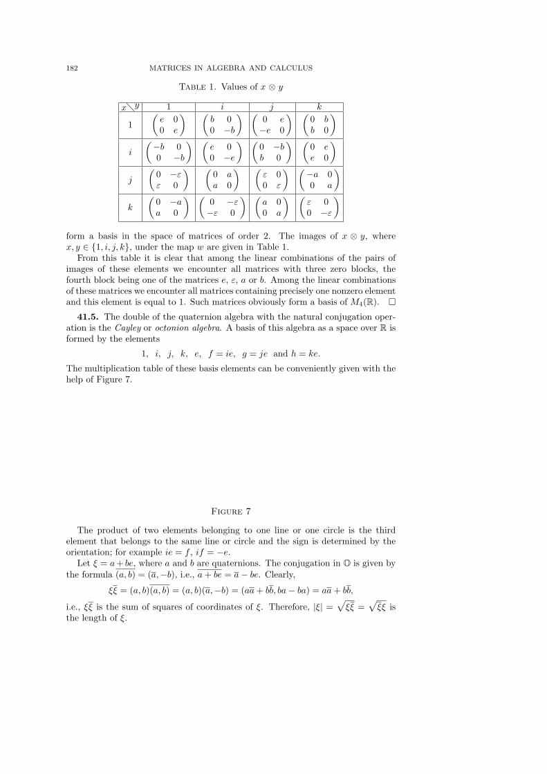
182 MATRICES IN ALGEBRA AND CALCULUS
Table 1. Values of x ⊗ y
xy 1 i j k
1(e 00 e
) (b 00 −b
) (0 e−e 0
) (0 bb 0
)
i
(−b 00 −b
) (e 00 −e
) (0 −bb 0
) (0 ee 0
)
j
(0 −εε 0
) (0 aa 0
) (ε 00 ε
) (−a 00 a
)
k
(0 −aa 0
) (0 −ε−ε 0
) (a 00 a
) (ε 00 −ε
)
form a basis in the space of matrices of order 2. The images of x ⊗ y, wherex, y ∈ 1, i, j, k, under the map w are given in Table 1.
From this table it is clear that among the linear combinations of the pairs ofimages of these elements we encounter all matrices with three zero blocks, thefourth block being one of the matrices e, ε, a or b. Among the linear combinationsof these matrices we encounter all matrices containing precisely one nonzero elementand this element is equal to 1. Such matrices obviously form a basis of M4(R). ¤
41.5. The double of the quaternion algebra with the natural conjugation oper-ation is the Cayley or octonion algebra. A basis of this algebra as a space over R isformed by the elements
1, i, j, k, e, f = ie, g = je and h = ke.
The multiplication table of these basis elements can be conveniently given with thehelp of Figure 7.
Figure 7
The product of two elements belonging to one line or one circle is the thirdelement that belongs to the same line or circle and the sign is determined by theorientation; for example ie = f , if = −e.
Let ξ = a+ be, where a and b are quaternions. The conjugation in O is given bythe formula (a, b) = (a,−b), i.e., a+ be = a− be. Clearly,
ξξ = (a, b)(a, b) = (a, b)(a,−b) = (aa+ bb, ba− ba) = aa+ bb,
i.e., ξξ is the sum of squares of coordinates of ξ. Therefore, |ξ| =√ξξ =
√ξξ is
the length of ξ.
41. QUATERNIONS AND CAYLEY NUMBERS. CLIFFORD ALGEBRAS 183
Theorem. |ξη| = |ξ| · |η|.Proof. For quaternions a similar theorem is proved quite simply, cf. 41.2. In
our case the lack of associativity is a handicap. Let ξ = a + be and η = u + ve,where a, b, u, v are quaternions. Then
|ξη|2 = (au− vb)(u a− bv) + (bu+ va)(ub+ a v).
Let us express a quaternion v in the form v = λ+ v1, where λ is a real number andv1 = −v1. Then
|ξη|2 = (au− λb+ v1b)(u a− λb− bv1)+
+ (bu+ λa+ v1a)(ub+ λa− av1).
Besides,|ξ|2|η|2 = (aa+ bb)(uu+ λ2 − v1v1).
Since uu and bb are real numbers, auu a = aauu and bbv1 = v1bb. Making use ofsimilar equalities we get
|ξη|2 − |ξ|2|η|2 = λ(−bu a− aub+ bu a+ aub)
+ v1(bu a+ aub)− (aub+ bu a)v1 = 0
because bua+ aub is a real number. ¤
41.5.1. Corollary. If ξ 6= 0, then ξ/|ξ|2 is a two-sided inverse for ξ.
41.5.2. Corollary. If ξ 6= 0 and η 6= 0 then ξη 6= 0.
The quaternion algebra is noncommutative and, therefore, O is a nonassociativealgebra. Instead, the elements of O satisfy
x(yy) = (xy)y, x(xy) = (xx)y and (yx)y = y(xy)
(see Problem 41.8). It is possible to show that any subalgebra of O generated bytwo elements is associative.
41.6. By analogy with the vector product in the space of purely imaginaryquaternions, we can define the vector product in the 7-dimensional space of purelyimaginary octanions. Let x and y be purely imaginary octanions. Their vectorproduct is the imaginary part of xy; it is denoted by x× y. Clearly,
x× y =12
(xy − xy) =12
(xy − yx).
It is possible to verify that the inner product (x, y) of octanions x and y is equal to12 (xy + yx) and for purely imaginary octanions we get (x, y) = − 1
2 (xy + yx).
Theorem. The vector product of purely imaginary octanions possesses the fol-lowing properties:
a) x× y ⊥ x, x× y ⊥ y;
184 MATRICES IN ALGEBRA AND CALCULUS
b) |x× y|2 = |x|2|y|2 − |(x, y)|2.
Proof. a) We have to prove that
(1) x(xy − yx) + (xy − yx)x = 0.
Since x(yx) = (xy)x (see Problem 41.8 b)), we see that (1) is equivalent to x(xy) =(yx)x. By Problem 41.8, a) we have x(xy) = (xx)y and (yx)x = y(xx). It remainsto notice that xx = −xx = −(x, x) is a real number.
b) We have to prove that
−(xy − yx)(xy − yx) = 4|x|2|y|2 − (xy + yx)(xy + yx),
i.e.,2|x|2|y|2 = (xy)(yx) + (yx)(xy).
Let a = xy. Then a = yx and
2|x|2|y|2 = 2(a, a) = aa+ aa = (xy)(yx) + (yx)(xy). ¤
41.7. The remaining part of this section will be devoted to the solution of thefollowing
Problem (Hurwitz-Radon). What is the maximal number of orthogonal oper-ators A1, . . . , Am in Rn satisfying the relations A2
i = −I and AiAj + AjAi = 0for i 6= j?
This problem might look quite artificial. There are, however, many importantproblems in one way or another related to quaternions or octonions that reduce tothis problem. (Observe that the operators of multiplication by i, j, . . . , h satisfy therequired relations.)
We will first formulate the answer and then tell which problems reduce to ourproblem.
Theorem (Hurwitz-Radon). Let us express an integer n in the form n = (2a+1)2b, where b = c+4d and 0 ≤ c ≤ 3. Let ρ(n) = 2c+8d; then the maximal numberof required operators in Rn is equal to ρ(n)− 1.
41.7.1. The product of quadratic forms. Let a = x1 + ix2 and b = y1 + iy2.Then the identity |a|2|b|2 = |ab|2 can be rewritten in the form
(x21 + x2
2)(y21 + y2
2) = z21 + z2
2 ,
where z1 = x1y1− x2y2 and z2 = x1y2 + x2y1. Similar identities can be written forquaternions and octonions.
Theorem. Let m and n be fixed natural numbers; let z1(x, y), . . . , zn(x, y) bereal bilinear functions of x = (x1, . . . , xm) and y = (y1, . . . , yn). Then the identity
(x21 + · · ·+ x2
m)(y21 + · · ·+ y2
n) = z21 + · · ·+ z2
n
41. QUATERNIONS AND CAYLEY NUMBERS. CLIFFORD ALGEBRAS 185
holds if and only if m ≤ ρ(n).
Proof. Let zi =∑j bij(x)yj , where bij(x) are linear functions. Then
z2i =
∑
j
b2ij(x)y2j + 2
∑
j<k
bij(x)bik(x)yjyk.
Therefore,∑i b
2ij = x2
1+· · ·+x2m and
∑j<k bij(x)bik(x) = 0. Let B(x) =
∥∥bij(x)∥∥n
1.
Then BT (x)B(x) = (x21 + · · · + x2
m)I. The matrix B(x) can be expressed in theform B(x) = x1B1 + · · ·+ xmBm. Hence,
BT (x)B(x) = x21B
T1 B1 + · · ·+ x2
mBTmBm +
∑
i<j
(BTi Bj +BTj Bi)xixj ;
therefore, BTi Bi = I and BTi Bj +BTj Bi = 0. The operators Bi are orthogonal andB−1i Bj = −B−1
j Bi for i 6= j.Let us consider the orthogonal operators A1, . . . , Am−1, where Ai = B−1
m Bi.Then B−1
m Bi = −B−1i Bm and, therefore, Ai = −A−1
i , i.e., A2i = −I. Besides,
B−1i Bj = −B−1
j Bi for i 6= j; hence,
AiAj = B−1m BiB
−1m Bj = −B−1
i BmB−1m Bj = B−1
j Bi = −AjAi.
It is also easy to verify that if the orthogonal operators A1, . . . , Am−1 are such thatA2i = −I and AiAj + AjAi = 0 then the operators B1 = A1, . . . , Bm−1 = Am−1,
Bm = I possess the required properties. To complete the proof of Theorem 41.7.1it remains to make use of Theorem 41.7. ¤
41.7.2. Normed algebras.
Theorem. Let a real algebra A be endowed with the Euclidean space structureso that |xy| = |x| · |y| for any x, y ∈ A. Then the dimension of A is equal to 1, 2,4 or 8.
Proof. Let e1, . . . , en be an orthonormal basis of A. Then
(x1e1 + · · ·+ xnen)(y1e1 + · · ·+ ynen) = z1e1 + · · ·+ znen,
where z1, . . . , zn are bilinear functions in x and y. The equality |z|2 = |x|2|y|2implies that
(x21 + · · ·+ x2
n)(y21 + · · ·+ y2
n) = z21 + · · ·+ z2
n.
It remains to make use of Theorem 41.7.1 and notice that ρ(n) = n if and only ifn = 1, 2, 4 or 8. ¤
41.7.3. The vector product.
Theorem ([Massey, 1983]). Let a bilinear operation f(v, w) = v × w ∈ Rn bedefined in Rn, where n ≥ 3; let f be such that v × w is perpendicular to v and wand |v × w|2 = |v|2|w|2 − (v, w)2. Then n = 3 or 7.
The product × determined by the above operator f is called the vector productof vectors.
186 MATRICES IN ALGEBRA AND CALCULUS
Proof. Consider the space Rn+1 = R ⊕ Rn and define a product in it by theformula
(a, v)(b, w) = (ab− (v, w), aw + bv + v × w),
where (v, w) is the inner product in Rn. It is easy to verify that in the resultingalgebra of dimension n + 1 the identity |xy|2 = |x|2|y|2 holds. It remains to makeuse of Theorem 41.7.2. ¤
Remark. In spaces of dimension 3 or 7 a bilinear operation with the aboveproperties does exist; cf. 41.6.
41.7.4. Vector fields on spheres. A vector field on a sphere Sn (say, unitsphere Sn = v ∈ Rn+1 | |v| = 1) is a map that to every point v ∈ Sn assigns avector F (v) in the tangent space to Sn at v. The tangent space to Sn at v consistsof vectors perpendicular to v; hence, F (v) ⊥ v. A vector field is said linear ifF (v) = Av for a linear operator A. It is easy to verify that Av ⊥ v for all v if andonly if A is a skew-symmetric operator (see Theorem 21.1.2). Therefore, any linearvector field on S2n vanishes at some point.
To exclude vector fields that vanish at a point we consider orthogonal operatorsonly; in this case |Av| = 1. It is easy to verify that an orthogonal operator A isskew-symmetric if and only if A2 = −I. Recall that an operator whose square isequal to −I is called a complex structure (see 10.4).
Vector fields F1, . . . , Fm are said to be linearly independent if the vectors F1(v),. . . , Fm(v) are linearly independent at every point v. In particular, the vectorfields corresponding to orthogonal operators A1, . . . , Am such that Aiv ⊥ Ajvfor all i 6= j are linearly independent. The equality (Aiv,Ajv) = 0 means that(v,ATi Ajv) = 0. Hence, ATi Aj + (ATi Aj)
T = 0, i.e., AiAj +AjAi = 0.Thus, to construct m linearly independent vector fields on Sn it suffices to in-
dicate orthogonal operators A1, . . . , Am in (n + 1)-dimensional space satisfyingthe relations A2
i = −I and AiAj + AjAi = 0 for i 6= j. Thus, we have proved thefollowing statement.
Theorem. On Sn−1, there exists ρ(n)− 1 linearly independent vector fields.
Remark. It is far more difficult to prove that there do not exist ρ(n) linearlyindependent continuous vector fields on Sn−1; see [Adams, 1962].
41.7.5. Linear subspaces in the space of matrices.
Theorem. In the space of real matrices of order n there is a subspace of dimen-sion m ≤ ρ(n) all nonzero matrices of which are invertible.
Proof. If the matrices A1, . . . , Am−1 are such that A2i = −I and AiAj +
AjAi = 0 for i 6= j then
(∑xiAi + xmI) (−∑
xiAi + xmI) = (x21 + · · ·+ x2
m)I.
Therefore, the matrix∑xiAi + xmI, where not all numbers x1, . . . , xm are zero,
is invertible. In particular, the matrices A1, . . . , Am−1, I are linearly indepen-dent. ¤
41. QUATERNIONS AND CAYLEY NUMBERS. CLIFFORD ALGEBRAS 187
41.8. Now, we turn to the proof of Theorem 41.7. Consider the algebra Cmover R with generators e1, . . . , em and relations e2
i = −1 and eiej + ejei = 0 fori 6= j. To every set of orthogonal matrices A1, . . . , Am satisfying A2
i = −I andAiAj + AjAi = 0 for i 6= j there corresponds a representation (see 42.1) of Cmthat maps the elements e1, . . . , em to orthogonal matrices A1, . . . , Am. In order tostudy the structure of Cm, we introduce an auxiliary algebra C ′m with generatorsε1, . . . , εm and relations ε2
i = 1 and εiεj + εjεi = 0 for i 6= j.The algebras Cm and C ′m are called Clifford algebraslifford algebra.
41.8.1. Lemma. C1∼= C, C2
∼= H, C ′1 ∼= R⊕ R and C ′2 ∼= M2(R).
Proof. The isomorphisms are explicitely given as follows:
C1 −→ C 1 7→ 1, e1 7→ i;C2 −→ H 1 7→ 1, e1 7→ i, e2 7→ j;
C ′1 −→ R⊕ R 1 7→ (1, 1), ε1 7→ (1,−1);
C ′2 −→M2(R) 1 7→(
1 00 1
), ε1 7→
(1 00 −1
), ε2 7→
(0 11 0
). ¤
Corollary. C⊗H ∼= M2(C).
Indeed, the complexifications of C2 and C ′2 are isomorphic. ¤41.8.2. Lemma. Ck+2
∼= C ′k ⊗ C2 and C ′k+2∼= Ck ⊗ C ′2.
Proof. The first isomorphism is given by the formulas
f(ei) = 1⊗ ei for i = 1, 2 and f(ei) = εi−2 ⊗ e1e2 for i ≥ 3.
The second isomorphism is given by the formulas
g(εi) = 1⊗ εi for i = 1, 2 and g(εi) = ei−2 ⊗ ε1ε2 for i ≥ 3. ¤
41.8.3. Lemma. Ck+4∼= Ck ⊗M2(H) and C ′k+4
∼= C ′k ⊗M2(H).
Proof. By Lemma 41.8.2 we have
Ck+4∼= C ′k+2 ⊗ C2
∼= Ck ⊗ C ′2 ⊗ C2.
SinceC ′2 ⊗ C2
∼= H⊗M2(R) ∼= M2(H),
we have Ck+4∼= Ck ⊗M2(H). Similarly, C ′k+4
∼= C ′k ⊗M2(H). ¤41.8.4. Lemma. Ck+8
∼= Ck ⊗M16(R).
Proof. By Lemma 41.8.3
Ck+8∼= Ck+4 ⊗M2(H) ∼= Ck ⊗M2(H)⊗M2(H).
Since H⊗H ∼= M4(R) (see 41.4), it follows that
M2(H)⊗M2(H) ∼= M2(M4(R)) ∼= M16(R). ¤
188 MATRICES IN ALGEBRA AND CALCULUS
Table 2
k 1 2 3 4Ck C H H⊕H M2(H)
C ′k R⊕ R M2(R) M2(C) M2(H)
k 5 6 7 8Ck M4(C) M8(R) M8(R)⊕M8(R) M16(R)
C ′k M2(H)⊕M2(H) M4(H) M8(C) M16(R)
Lemmas 41.8.1–41.8.3 make it possible to calculate Ck for 1 ≤ k ≤ 8. Forexample,
C5∼= C1 ⊗M2(H) ∼= C⊗M2(H) ∼= M2(C⊗H) ∼= M2(M2(C)) ∼= M4(C);
C6∼= C2 ⊗M2(H) ∼= M2(H⊗H) ∼= M8(R),
etc. The results of calculations are given in Table 2.Lemma 41.8.4 makes it possible now to calculate Ck for any k. The algebras C1,
. . . , C8 have natural representations in the spaces C, H, H, H2, C4, R8, R8 and R16
whose dimensions over R are equal to 2, 4, 4, 8, 8, 8, 8 and 16. Besides, under thepassage from Ck to Ck+8 the dimension of the space of the natural representationis multiplied by 16. The simplest case-by-case check indicates that for n = 2k thelargest m for which Cm has the natural representation in Rn is equal to ρ(n)− 1.
Now, let us show that under these natural representations of Cm in Rn theelements e1, . . . , em turn into orthogonal matrices if we chose an appropriate basisin Rn. First, let us consider the algebra H = R4. Let us assign to an element a ∈ Hthe map x 7→ ax of the space H into itself. If we select basis 1, i, j, k in the spaceH = R4, then to elements 1, i, j, k the correspondence indicated assigns orthogonalmatrices. We may proceed similarly in case of the algebra C = R2.
We have shown how to select bases in C = R2 and H = R4 in order for theelements ei and εj of the algebras C1, C2, C
′1 and C ′2 were represented by orthogonal
matrices. Lemmas 41.8.2-4 show that the elements ei and εj of the algebras Cmand C ′m are represented by matrices obtained consequtevely with the help of theKronecker product, and the initial matrices are orthogonal. It is clear that theKronecker product of two orthogonal matrices is an orthogonal matrix (cf. 27.4).
Let f : Cm −→ Mn(R) be a representation of Cm under which the elementse1, . . . , em turn into orthogonal matrices. Then f(1 ·ei) = f(1)f(ei) and the matrixf(ei) is invertible. Hence, f(1) = f(1 · ei)f(ei)−1 = I is the unit matrix. Thealgebra Cm is either of the form Mp(F ) or of the form Mp(F ) ⊕Mp(F ), whereF = R,C or H. Therefore, if f is a representation of Cm such that f(1) = I, thenf is completely reducible and its irreducible components are isomorphic to F p (see42.1); so its dimension is divisible by p. Therefore, for any n the largest m forwhich Cm has a representation in Rn such that f(1) = I is equal to ρ(n)− 1.
Problems
41.1. Prove that the real part of the product of quaternions x1i + y1j + z1kand x2i + y2j + z2k is equal to the inner product of the vectors (x1, y1, z1) and(x2, y2, z2) taken with the minus sign, and that the imaginary part is equal to theirvector product.
42. REPRESENTATIONS OF MATRIX ALGEBRAS 189
41.2. a) Prove that a quaternion q is purely imaginary if and only if q2 ≤ 0.b) Prove that a quaternion q is real if and only if q2 ≥ 0.41.3. Find all solutions of the equation q2 = −1 in quaternions.41.4. Prove that a quaternion that commutes with all purely imaginary quater-
nions is real.41.5. A matrix A with quaternion elements can be represented in the form
A = Z1 + Z2j, where Z1 and Z2 are complex matrices. Assign to a matrix A the
matrix Ac =(
Z1 Z2
−Z2 Z1
). Prove that (AB)c = AcBc.
41.6. Consider the map in the space R4 = H which sends a quaternion x to qx,where q is a fixed quaternion.
a) Prove that this map sends orthogonal vectors to orthogonal vectors.b) Prove that the determinant of this map is equal to |q|4.41.7. Given a tetrahedron ABCD prove with the help of quaternions that
AB · CD +BC ·AD ≥ AC ·BD.
41.8. Let x and y be octonions. Prove that a) x(yy) = (xy)y and x(xy) = (xx)y;b) (yx)y = y(xy).
42. Representations of matrix algebras
42.1. Let A be an associative algebra and Mat(V ) the associative algebra oflinear transformations of a vector space V . A homomorphism f : A −→ Mat(V )of associative algebras is called a representation of A. Given a homomorphism fwe define the action of A in V by the formula av = f(a)v. We have (ab)v = a(bv).Thus, the space V is an A-module.
A subspace W ⊂ V is an invariant subspace of the representation f if AW ⊂W , i.e., if W is a submodule of the A-module V . A representation is said to beirreducible if any nonzero invariant subspace of it coincides with the whole spaceV . A representation f : A −→ Mat(V ) is called completely reducible if the spaceV is the direct sum of invariant subspaces such that the restriction of f to each ofthem is irreducible.
42.1.1. Theorem. Let A = Mat(V n) and f : A −→ Mat(Wm) a representationsuch that f(In) = Im. Then Wm = W1 ⊕ · · · ⊕Wk, where the Wi are invariantsubspaces isomorphic to V n.
Proof. Let e1, . . . , em be a basis of W . Since f(In)ei = ei, it follows thatW ⊂ Span(Ae1, . . . , Aem). It is possible to represent the space of A in the form ofthe direct sum of subspaces Fi consisting of matrices whose columns are all zero,except the ith one. Clearly, AFi = Fi and if a is a nonzero element of Fi thenAa = Fi. The space W is the sum of spaces Fiej . These spaces are invariant, sinceAFi = Fi. If x = aej , where a ∈ Fi and x 6= 0, then Ax = Aaej = Fiej .
Therefore, any two spaces of the form Fiej either do not have common nonzeroelements or coincide. It is possible to represent W in the form of the direct sum ofcertain nonzero subspaces Fiej . For this we have to add at each stage subspacesnot contained in the direct sum of the previously chosen subspaces. It remains todemonstrate that every nonzero space Fiej is isomorphic to V . Consider the maph : Fi −→ Fiej for which h(a) = aej . Clearly, AKerh ⊂ Kerh. Suppose thatKerh 6= 0. In Kerh, select a nonzero element a. Then Aa = Fi. On the other
190 MATRICES IN ALGEBRA AND CALCULUS
hand, Aa ⊂ Kerh. Therefore, Kerh = Fi, i.e., h is the zero map. Hence, either his an isomorphism or the zero map.
This proof remains valid for the algebra of matrices over H, i.e., when V andW are spaces over H. Note that if A = Mat(V n), where V n is a space over H andf : A −→ Mat(Wm) a representation such that f(In) = Im, then Wm necessarilyhas the structure of a vector space over H. Indeed, the multiplication of elementsof Wm by i, j, k is determined by operators f(iIn), f(jIn), f(kIn). ¤
In section §41 we have made use of not only Theorem 42.1.1 but also of thefollowing statement.
42.1.2. Theorem. Let A = Mat(V n) ⊕Mat(V n) and f : A −→ Mat(Wm) arepresentation such that f(In) = Im. Then Wm = W1 ⊕ · · · ⊕Wk, where the Wi
are invariant subspaces isomorphic to V n.
Proof. Let Fi be the set of matrices defines in the proof of Theorem 42.1.1.The space A can be represented as the direct sum of its subspaces F 1
i = Fi⊕ 0 andF 2i = 0⊕Fi. Similarly to the proof of Theorem 42.1.1 we see that the space W can
be represented as the direct sum of certain nonzero subspaces F ki ej each of whichis invariant and isomorphic to V n. ¤
43. The resultant
43.1. Consider polynomials f(x) =∑ni=0 aix
n−i and g(x) =∑mi=0 bix
m−i,where a0 6= 0 and b0 6= 0. Over an algebraically closed field, f and g have acommon divisor if and only if they have a common root. If the field is not alge-braically closed then the common divisor can happen to be a polynomial withoutroots.
The presence of a common divisor for f and g is equivalent to the fact that thereexist polynomials p and q such that fq = gp, where deg p ≤ n−1 and deg q ≤ m−1.Let q = u0x
m−1 + · · ·+ um−1 and p = v0xn−1 + · · ·+ vn−1. The equality fq = gp
can be expressed in the form of a system of equations
a0u0 = b0v0
a1u0 + a0u1 = b1v0 + b0v1
a2u0 + a1u1 + a0u2 = b2v0 + b1v1 + b0v2
. . . . . .
The polynomials f and g have a common root if and only if this system ofequations has a nonzero solution (u0, u1, . . . , v0, v1, . . . ). If, for example, m = 3and n = 2, then the determinant of this system is of the form
∣∣∣∣∣∣∣∣∣
a0 0 0 −b0 0a1 a0 0 −b1 −b0a2 a1 a0 −b2 −b10 a2 a1 −b3 −b20 0 a2 0 −b3
∣∣∣∣∣∣∣∣∣= ±
∣∣∣∣∣∣∣∣∣
a0 a1 a2 0 00 a0 a1 a2 00 0 a0 a1 a2
b0 b1 b2 b3 00 b0 b1 b2 b3
∣∣∣∣∣∣∣∣∣= ±|S(f, g)|.
The matrix S(f, g) is called Sylvester’s matrix of polynomials f and g. The deter-minant of S(f, g) is called the resultant of f and g and is denoted by R(f, g). It
43. THE RESULTANT 191
is clear that R(f, g) is a homogeneous polynomial of degree m with respect to thevariables ai and of degree n with respect to the variables bj . The polynomials fand g have a common divisor if and only if the determinant of the above system iszero, i.e., if R(f, g) = 0.
The resultant has a number of applications. For example, given polynomialrelations P (x, z) = 0 and Q(y, z) = 0 we can use the resultant in order to obtaina polynomial relation R(x, y) = 0. Indeed, consider given polynomials P (x, z) andQ(y, z) as polynomials in z considering x and y as constant parameters. Then theresultant R(x, y) of these polynomials gives the required relation R(x, y) = 0.
The resultant also allows one to reduce the problem of solution of a system ofalgebraic equations to the search of roots of polynomials. In fact, let P (x0, y0) = 0and Q(x0, y0) = 0. Consider P (x, y) and Q(x, y) as polynomials in y. At x = x0
they have a common root y0. Therefore, their resultant R(x) vanishes at x = x0.
43.2. Theorem. Let xi be the roots of a polynomial f and let yj be the rootsof a polynomial g. Then
R(f, g) = am0 bn0
∏(xi − yj) = am0
∏g(xi) = bn0
∏f(yj).
Proof. Since f = a0(x− x1) . . . (x− xn), then ak = ±a0σk(x1, . . . , xn), whereσk is an elementary symmetric function. Similarly, bk = ±b0σk(y1, . . . , ym). Theresultant is a homogeneous polynomial of degree m with respect to variables ai andof degree n with respect to the bj ; hence,
R(f, g) = am0 bn0P (x1, . . . , xn, y1, . . . , ym),
where P is a symmetric polynomial in the totality of variables x1, . . . , xn andy1, . . . , ym which vanishes for xi = yj . The formula
xki = (xi − yj)xk−1i + yjx
k−1i
shows that
P (x1, . . . , ym) = (xi − yj)Q(x1, . . . , ym) +R(x1, . . . , xi, . . . , ym).
Substituting xi = yj in this equation we see that R(x1, . . . , xi, . . . , ym) is identicallyequal to zero, i.e., R is the zero polynomial. Similar arguments demonstrate thatP is divisible by S = am0 b
n0
∏(xi − yj).
Since g(x) = b0∏mj=1(x−yj), it follows that
∏ni=1 g(xi) = bn0
∏i,j(xi−yj); hence,
S = am0
n∏
i=1
g(xi) = am0
n∏
i=1
(b0xmi + b1xm−1i + · · ·+ bm)
is a homogeneous polynomial of degree n with respect to b0, . . . , bm.For the variables a0, . . . , an our considerations are similar. It is also clear that the
symmetric polynomial am0∏
(b0xmi +b1xm−1i +· · ·+bm) is a polynomial in a0, . . . , an,
b0, . . . , bm. Hence, R(a0, . . . , bm) = λS(a0, . . . , bm), where λ is a number. On theother hand, the coefficient of
∏xmi in the polynomials am0 b
n0P (x1, . . . , ym) and
S(x1, . . . , ym) is equal to am0 bn0 ; hence, λ = 1. ¤
192 MATRICES IN ALGEBRA AND CALCULUS
43.3. Bezout’s matrix. The size of Sylvester’s matrix is too large and, there-fore, to compute the resultant with its help is inconvenient. There are many variousways to diminish the order of the matrix used to compute the resultant. For ex-ample, we can replace the polynomial g by the remainder of its division by f (seeProblem 43.1).
There are other ways to diminish the order of the matrix used for the computa-tions.
Suppose that m = n.
Let us express Sylvester’s matrix in the form(A1 A2
B1 B2
), where the Ai, Bi are
square matrices. It is easy to verify that
A1B1 =
c0 c1 . . . cn−1 cn0 c0 . . . cn−2 cn−1
......
. . ....
...0 0 . . . c0 c10 0 . . . 0 c0
= B1A1, where ck =k∑
i=0
aibk−i;
hence, (I 0−B1 A1
)(A1 A2
B1 B2
)=
(A1 A2
0 A1B2 −B1A2
)
and since |A1| = an0 , then R(f, g) = |A1B2 −B1A2|.Let cpq = apbq − aqbp. It is easy to see that A1B2 − B1A2 =
∥∥wij∥∥n
1, where
wij =∑cpq and the summation runs over the pairs (p, q) such that p+q = n+j−i,
p ≤ n−1 and q ≥ j. Since cαβ + cα+1,β−1 + · · ·+ cβα = 0 for α ≤ β, we can confineourselves to the pairs for which p ≤ min(n − 1, j − 1). For example, for n = 4 weget the matrix
c04 c14 c24 c34
c03 c04 + c13 c14 + c23 c24
c02 c03 + c12 c04 + c13 c14
c01 c02 c03 c04
.
Let J = antidiag(1, . . . , 1), i.e., J =∥∥aij
∥∥n1, where aij =
1 for i+ j = n+ 10 otherwise
.
Then the matrix Z = |wij |n1J is symmetric. It is called the Bezoutian or Bezout’smatrix of f and g.
43.4. Barnett’s matrix. Let us describe one more way to diminish the order ofthe matrix to compute the resultant ([Barnett, 1971]). For simplicity, let us assumethat a0 = 1, i.e., f(x) = xn+a1x
n−1+· · ·+an and g(x) = b0xm+b1xm−1+· · ·+bm.
To f and g assign Barnett’s matrix R = g(A), where
A =
0 1 0 . . . 00 0 1 . . . 0...
.... . . . . .
......
......
. . . 0
0 0 0. . . 1
−an −an−2 −an−3 . . . −a1
.
43. THE RESULTANT 193
43.4.1. Theorem. detR = R(f, g).
Proof. Let β1, . . . , βm be the roots of g. Then g(x) = b0(x− β1) . . . (x− βm).Hence, g(A) = b0(A−β1I) . . . (A−βmI). Since det(A−λI) =
∏i(αi−λ) (see 1.5),
then det g(A) = bm0∏
(αi − βi) = R(f, g). ¤43.4.2. Theorem. For m ≤ n it is possible to calculate the matrix R in the
following recurrent way. Let r1, . . . , rn be the rows of R. Then
r1 =
(bm, bm−1, . . . , b1, b0, 0, . . . , 0) for m < n
(dn, . . . , d1) for m = n,
where di = bi − b0ai. Besides, ri = ri−1A for i = 2, . . . , n.
Proof. Let ei = (0, . . . , 1, . . . , 0), where 1 occupies the ith slot. For k < n thefirst row of Ak is equal to ek+1. Therefore, the structure of r1 for m < n is obvious.For m = n we have to make use of the identity An +
∑ni=1 aiA
n−i = 0.Since ei = ei−1A for i = 2, . . . , n, it follows that
ri = eiR = ei−1AR = ei−1RA = ri−1A. ¤
43.4.3. Theorem. The degree of the greatest common divisor of f and g isequal to n− rankR.
Proof. Let β1, . . . , βs be the roots of g with multiplicities k1, . . . , ks, respec-tively. Then g(x) = b0
∏(x − βi)ki and R = g(A) = b0
∏i(A − βiI)ki . Under
the passage to the basis in which the matrix A is of the Jordan normal form J ,the matrix R is replaced by b0
∏(J − βiI)ki . The characteristic polynomial of A
coincides with the minimal polynomial and, therefore, if βi is a root of multiplicityli of f , then the Jordan block Ji of J corresponding to the eigenvalue βi is of orderli. It is also clear that
rank(Ji − βiI)ki = li −min(ki, li).
Now, considering the Jordan blocks of J separately, we easily see that n −rankR =
∑i min(ki, li) and the latter sum is equal to the degree of the great-
est common divisor of f and g. ¤43.5. Discriminant. Let x1, . . . , xn be the roots of f(x) = a0x
n+ · · ·+an andlet a0 6= 0. The number D(f) = a2n−2
0
∏i<j(xi−xj) is called the discriminant of f .
It is also clear that D(f) = 0 if and only if f has multiple roots, i.e., R(f, f ′) = 0.
43.5.1. Theorem. R(f, f ′) = ±a0D(f).
Proof. By Theorem 43.2 R(f, f ′) = an−10
∏i f′(xi).
It is easy to verify that if xi is a root of f , then f ′(xi) = a0
∏j 6=i(xj − xi).
Therefore,
R(f, f ′) = a2n−10
∏
j 6=i(xi − xj) = ±a2n−1
0
∏
i<j
(xi − xj)2. ¤
194 MATRICES IN ALGEBRA AND CALCULUS
Corollary. The discriminant is a polynomial in the coefficients of f .
43.5.2. Theorem. Any matrix is the limit of matrices with simple (i.e., nonmultiple)eigenvalues.
Proof. Let f(x) be the characteristic polynomial of a matrix A. The polyno-mial f has multiple roots if and only if D(f) = 0. Therefore, we get an algebraicequation for elements of A. The restriction of the equation D(f) = 0 to the lineλA + (1 − λ)B, where B is a matrix with simple eigenvalues, has finitely manyroots. Therefore, A is the limit of matrices with simple eigenvalues. ¤
Problems
43.1. Let r(x) be the remainder of the division of g(x) by f(x) and let deg r(x) =k. Prove that R(f, g) = am−k0 R(f, r).
43.2. Let f(x) = a0xn + · · · + an, g(x) = b0x
m + · · · + bm and let rk(x) =ak0x
n−1 + ak1xn−2 + · · · + ak,n−1 be the remainder of the division of xkg(x) by
f(x). Prove that
R(f, g) = am0
∣∣∣∣∣∣∣
an−1,0 . . . an−1,n−1
......
...a00 . . . a0,n−1
∣∣∣∣∣∣∣.
43.3. The characteristic polynomials of matrices A and B of size n×n and m×mare equal to f and g, respectively. Prove that the resultant of the polynomials fand g is equal to the determinant of the operator X 7→ AX −XB in the space ofmatrices of size n×m.
43.4. Let α1, . . . , αn be the roots of a polynomial f(x) =∑ni=0 aix
n−i andsk = αk1 + · · ·+ αkn. Prove that D(f) = a2n−2
0 detS, where
S =
s0 s1 . . . sn−1
s1 s2 . . . sn...
......
...sn−1 sn . . . s2n−2
.
44. The generalized inverse matrix. Matrix equations
44.1. A matrix X is called a generalized inverse for a (not necessarily square)matrix A, if XAX = X, AXA = A and the matrices AX and XA are Hermitianones. It is easy to verify that for an invertible A its generalized inverse matrixcoincides with the inverse matrix.
44.1.1. Theorem. A matrix X is a generalized inverse for A if and only if thematrices P = AX and Q = XA are Hermitian projections onto ImA and ImA∗,respectively.
Proof. First, suppose that P and Q are Hermitian projections to ImA andImA∗, respectively. If v is an arbitrary vector, then Av ∈ ImA and, therefore,PAv = Av, i.e., AXAv = Av. Besides, Xv ∈ ImXA = ImA∗; hence, QXv = Xv,i.e., XAXv = Xv.
Now, suppose that X is a generalized inverse for A. Then P 2 = (AXA)X =AX = P and Q2 = (XAX)A = XA = Q, where P and Q are Hermitian matrices.It remains to show that ImP = ImA and ImQ = ImA∗. Since P = AX and
44. THE GENERALIZED INVERSE MATRIX. MATRIX EQUATIONS 195
Q = Q∗ = A∗X∗, then ImP ⊂ ImA and ImQ ⊂ ImA∗. On the other hand,A = AXA = PA and A∗ = A∗X∗A∗ = Q∗A∗ = QA∗; hence, ImA ⊂ ImP andImA∗ ⊂ ImQ. ¤
44.1.2. Theorem (Moore-Penrose). For any matrix A there exists a uniquegeneralized inverse matrix X.
Proof. If rankA = r then A can be represented in the form of the product ofmatrices C and D of size m × r and r × n, respectively, where ImA = ImC andImA∗ = ImD∗. It is also clear that C∗C and DD∗ are invertible. Set
X = D∗(DD∗)−1(C∗C)−1C∗.
Then AX = C(C∗C)−1C∗ and XA = D∗(DD∗)−1D, i.e., the matrices AX andXA are Hermitian projections onto ImC = ImA and ImD∗ = ImA∗, respectively,(see 25.3) and, therefore, X is a generalized inverse for A.
Now, suppose that X1 and X2 are generalized inverses for A. Then AX1 andAX2 are Hermitian projections onto ImA, implying AX1 = AX2. Similarly, X1A =X2A. Therefore,
X1 = X1(AX1) = (X1A)X2 = X2AX2 = X2. ¤
The generalized inverse of A will be denoted5 by A“−1”.
44.2. The generalized inverse matrix A“−1” is applied to solve systems of linearequations, both inconsistent and consistent. The most interesting are its applica-tions solving inconsistent systems.
44.2.1. Theorem. Consider a system of linear equations Ax = b. The value|Ax− b| is minimal for x such that Ax = AA“−1”b and among all such x the leastvalue of |x| is attained at the vector x0 = A“−1”b.
Proof. The operator P = AA“−1” is a projection and therefore, I − P is alsoa projection and Im(I −P ) = KerP (see Theorem 25.1.2). Since P is an Hermitianoperator, KerP = (ImP )⊥. Hence,
Im(I − P ) = KerP = (ImP )⊥ = (ImA)⊥,
i.e., for any vectors x and y the vectors Ax and (I − AA“−1”)y are perpendicularand
|Ax+ (I −AA“−1”)y|2 = |Ax|2 + |y −AA“−1”y|2.Similarly,
|A“−1”x+ (I −A“−1”A)y|2 = |A“−1”x|2 + |y −A“−1”Ay|2.
SinceAx− b = A(x−A“−1”b)− (I −AA“−1”)b,
5There is no standard notation for the generalized inverse of a matrix A. Many authors tookafter R. Penrose who denoted it by A+ which is confusing: might be mistaken for the Hermitianconjugate. In the original manuscript of this book Penrose’s notation was used. I suggest a moredynamic and noncontroversal notation approved by the author. Translator.
196 MATRICES IN ALGEBRA AND CALCULUS
it follows that
|Ax− b|2 = |Ax−AA“−1”b|2 + |b−AA“−1”b|2 ≥ |b−AA“−1”b|2
and equality is attained if and only if Ax = AA“−1”b. If Ax = AA“−1”b, then
|x|2 = |A“−1”b+ (I −A“−1”A)x|2 = |A“−1”b|2 + |x−A“−1”Ax|2 ≥ |A“−1”b|2
and equality is attained if and only if
x = A“−1”Ax = A“−1”AA“−1”b = A“−1”b. ¤
Remark. The equality Ax = AA“−1”b is equivalent to the equality A∗Ax =A∗x. Indeed, if Ax = AA“−1”b then A∗b = A∗(A“−1”)∗A∗b = A∗AA“−1”b = A∗Axand if A∗Ax = A∗b then
Ax = AA“−1”Ax = (A“−1”)∗A∗Ax = (A“−1”)∗A∗b = AA“−1”b.
With the help of the generalized inverse matrix we can write a criterion forconsistency of a system of linear equations and find all its solutions.
44.2.2. Theorem. The matrix equation
(1) AXB = C
has a solution if and only if AA“−1”CB“−1”B = C. The solutions of (1) are of theform
X = A“−1”CB“−1” + Y −A“−1”AY BB“−1”, where Y is an arbitrary matrix.
Proof. If AXB = C, then
C = AXB = AA“−1”(AXB)B“−1”B = AA“−1”CB“−1”B.
Conversely, if C = AA“−1”CB“−1”B, then X0 = A“−1”CB“−1” is a particularsolution of the equation
AXB = C.
It remains to demonstrate that the general solution of the equation AXB = 0 is ofthe form X = Y −A“−1”AY BB“−1”. Clearly, A(Y −A“−1”AY BB“−1”)B = 0. Onthe other hand, if AXB = 0 then X = Y −A“−1”AY BB“−1”, where Y = X. ¤
Remark. The notion of generalized inverse matrix appeared independently inthe papers of [Moore, 1935] and [Penrose, 1955]. The equivalence of Moore’s andPenrose’s definitions was demonstrated in the paper [Rado, 1956].
44. THE GENERALIZED INVERSE MATRIX. MATRIX EQUATIONS 197
44.3. Theorem ([Roth, 1952]). Let A ∈Mm,m, B ∈Mn,n and C ∈Mm,n.a) The equation AX − XB = C has a solution X ∈ Mm,n if and only if the
matrices(A 00 B
)and
(A C0 B
)are similar.
b) The equation AX − Y B = C has a solution X,Y ∈ Mm,n if and only if
matrices(A 00 B
)and
(A C0 B
)are of the same rank.
Proof (Following [Flanders, Wimmer, 1977]). a) Let K =(P QR S
), where
P ∈ Mm,m and S ∈ Mn,n. First, suppose that the matrices from the theorem aresimilar. For i = 0, 1 consider the maps ϕi : Mm,n −→Mm,n given by the formulas
ϕ0(K) =(A 00 B
)K −K
(A 00 B
)=
(AP − PA AQ−QBBR−RA BS − SB
),
ϕ1(K) =(A C0 B
)K −K
(A 00 B
)=
(AP + CR− PA AQ+ CS −QB
BR−RA BS − SB).
The equations FK = KF and GFG−1K ′ = K ′F have isomorphic spaces of solu-tions; this isomorphism is given by the formula K = G−1K ′. Hence, dim Kerϕ0 =dim Kerϕ1. If K ∈ Kerϕi, then BR = RA and BS = SB. Therefore, we canconsider the space
V = (R,S) ∈Mn,m+n | BR = RA, BS = SB
and determine the projection µi : Kerϕi −→ V , where µi(X) = (R,S). It is easyto verify that
Kerµi = (P Q0 0
)| AP = PA, AQ = QB.
For µ0 this is obvious and for µ1 it follows from the fact that CR = 0 and CS = 0since R = 0 and S = 0.
Let us prove that Imµ0 = Imµ1. If (R,S) ∈ V , then(
0 0R S
)∈ Kerϕ0. Hence,
Imµ0 = V and, therefore, Imµ1 ⊂ Imµ0. On the other hand,
dim Imµ0 + dim Kerµ0 = dim Kerϕ0 = dim Kerϕ1 = dim Imµ1 + dim Kerµ1.
The matrix(I 00 −I
)belongs to Kerϕ0 and, therefore, (0,−I) ∈ Imµ0 = Imµ1.
Hence, there is a matrix of the form(P Q0 −I
)in Kerϕ1. Thus, AQ+CS−QB = 0,
where S = −I. Therefore, X = Q is a solution of the equation AX −XB = C.Conversely, if X is a solution of this equation, then(A 00 B
)(I X0 I
)=
(A AX0 B
)=
(A C +XB0 B
)=
(I X0 I
)(A C0 B
)
and, therefore(I X0 I
)−1 (A 00 B
)(I X0 I
)=
(A C0 B
).
198 MATRICES IN ALGEBRA AND CALCULUS
b) First, suppose that the indicated matrices are of the same rank. For i = 0, 1consider the map ψi : Mm+n,2(m+n) −→Mm+n,m+n given by formulas
ψ0(U,W ) =(A 00 B
)U −W
(A 00 B
)=
(AU11 −W11A AU12 −W12BBU21 −W21A BU22 −W22B
),
ψ1(U,W ) =(A C0 B
)U −W
(A 00 B
)
=(AU11 + CU21 −W11A AU12 + CU22 −W12B
BU21 −W21A BU22 −W22B
),
where
U =(U11 U12
U21 U22
)and W =
(W11 W12
W21 W22
).
The spaces of solutions of equations FU = WF and GFG−1U ′ = W ′F are isomor-phic and this isomorphism is given by the formulas U = G−1U ′ and W = G−1W ′.Hence, dim Kerψ0 = dim Kerψ1.
Consider the space
Z = (U21, U22W21,W22) | BU21 = W21A, BU22 = W22B
and define a map νi : Kerϕi −→ Z, where νi(U,W ) = (U21, U22,W21,W22). ThenIm ν1 ⊂ Im ν0 = Z and Ker ν1 = Ker ν0. Therefore, Im ν1 = Im ν0. The matrix
(U,W ), where U = W =(I 00 −I
), belongs to Kerψ0. Hence, Kerψ1 also contains
an element for which U22 = −I. For this element the equality AU12+CU22 = W12Bis equivalent to the equality AU12 −W12B = C.
Conversely, if a solution X,Y of the given equation exists, then(I −Y0 I
)(A 00 B
)(I X0 I
)=
(A AX − Y B0 B
)=
(A C0 B
). ¤
Problems
44.1. Prove that if C = AX = Y B, then there exists a matrix Z such thatC = AZB.
44.2. Prove that any solution of a system of matrix equations AX = 0, BX = 0is of the form X = (I −A“−1”A)Y (I −BB“−1”), where Y is an arbitrary matrix.
44.3. Prove that the system of equations AX = C, XB = D has a solution if andonly if each of the equations AX = C and XB = D has a solution and AD = CB.
45. Hankel matrices and rational functions
Consider a proper rational function
R(z) =a1z
m−1 + · · ·+ amb0zm + b1zm−1 + · · ·+ bm
,
where b0 6= 0. It is possible to expand this function in a series
R(z) = s0z−1 + s1z
−2 + s2z−3 + . . . ,
45. HANKEL MATRICES AND RATIONAL FUNCTIONS 199
where
(1)
b0s0 = a1,
b0s1 + b1s0 = a2,
b0s2 + b1s1 + b2s0 = a3,
. . . . . . . . . . . . . . . . . .
b0sm−1 + · · ·+ bm−1s0 = am
Besides, b0sq + · · ·+ bmsq−m = 0 for q ≥ m. Thus, for all q ≥ m we have
(2) sq = α1sq−1 + · · ·+ αmsq−m,
where αi = −bi/b0. Consider the infinite matrix
S =
∥∥∥∥∥∥∥∥
s0 s1 s2 . . .s1 s2 s3 . . .s2 s3 s4 . . ....
...... · · ·
∥∥∥∥∥∥∥∥.
A matrix of such a form is called a Hankel matrix. Relation (2) means that the(m + 1)th row of S is a linear combination of the first m rows (with coefficientsα1, . . . , αm). If we delete the first element of each of these rows, we see that the(m+2)th row of S is a linear combination of the m rows preceding it and therefore,the linear combination of the first m rows. Continuing these arguments, we deducethat any row of the matrix S is expressed in terms of its first m rows, i.e., rankS ≤m.
Thus, if the series
(3) R(z) = s0z−1 + s1z
−2 + s2z−3 + . . .
corresponds to a rational function R(z) then the Hankel matrix S constructed froms0, s1, . . . is of finite rank.
Now, suppose that the Hankel matrix S is of finite rank m. Let us construct fromS a series (3). Let us prove that this series corresponds to a rational function. Thefirst m + 1 rows of S are linearly dependent and, therefore, there exists a numberh ≤ m such that the m+ 1-st row can be expressed linearly in terms of the first mrows. As has been demonstrated, in this case all rows of S are expressed in termsof the first h rows. Hence, h = m. Thus, the numbers si are connected by relation(2) for all q ≥ m. The coefficients αi in this relation enable us to determine thenumbers b0 = 1, b1 = α1, . . . , bm = αm. Next, with the help of relation (1) we candetermine the numbers a1, . . . , am. For the numbers ai and bj determined in thisway we have
s0
z+s1
z2+ · · · = a1z
m−1 + · · ·+ amb0zm + · · ·+ bm
,
i.e., R(z) is a rational function.
Remark. Matrices of finite size of the form
s0 s1 . . . sns1 s2 . . . sn+1
......
......
sn sn+1 . . . s2n
.
200 MATRICES IN ALGEBRA AND CALCULUS
are also sometimes referred to as Hankel matrices. Let J = antidiag(1, . . . , 1), i.e.,
J =∥∥aij
∥∥n0, where aij =
1 for i+ j = n,
0 otherwise.If H is a Hankel matrix, then the
matrix JH is called a Toeplitz matrix; it is of the form
a0 a1 a2 . . . ana−1 a0 a1 . . . an−1
a−2 a−1 a0 . . . an−2
......
......
...a−n a−n+1 a−n+2 . . . a0
.
46. Functions of matrices. Differentiation of matrices
46.1. By analogy with the exponent of a number, we can define the expontentof a matrix A to be the sum of the series
∞∑
k=0
Ak
k!.
Let us prove that this series converges. If A and B are square matrices of ordern and |aij | ≤ a, |bij | ≤ b, then the absolute value of each element of AB doesnot exceed nab. Hence, the absolute value of the elements of Ak does not exceednk−1ak = (na)k/n and, since 1
n
∑∞k=0
(na)k
k! = 1ne
na, the series∑∞k=0
Ak
k! convergesto a matrix denoted by eA = expA; this matrix is called the exponent of A.
If A1 = P−1AP , then Ak1 = P−1AkP . Therefore, exp(P−1AP ) = P−1(expA)P .Hence, the computation of the exponent of an arbitrary matrix reduces to thecomputation of the exponent of its Jordan blocks.
Let J = λI +N be a Jordan block of order n. Then
(λI +N)k =k∑
m=0
(k
m
)λk−mNm.
Hence,
exp(tJ) =∞∑
k=0
tkJk
k!=
∞∑
k,m=0
tk(km
)λk−mNm
k!
=∞∑m=0
∞∑
k=m
(λt)k−m
(k −m)!tmNm
m!=∞∑m=0
tm
m!eλtNm =
n−1∑m=0
tm
m!eλtNm,
since Nm = 0 for m ≥ n.By reducing a matrix A to the Jordan normal form we get the following state-
ment.
46.1.1. Theorem. If the minimal polynomial of A is equal to
(x− λ1)n1 . . . (x− λk)nk ,
then the elements of eAt are of the form p1(t)eλ1t + · · · + pk(t)eλkt, where pi(t) isa polynomial of degree not greater than ni − 1.
46. FUNCTIONS OF MATRICES. DIFFERENTIATION OF MATRICES 201
46.1.2. Theorem. det(eA) = etrA.
Proof. We may assume that A is an upper triangular matrix with elementsλ1, . . . , λn on the diagonal. Then Ak is an upper triangular matrix with elementsλk1
1 , . . . , λknn of the diagonal. Hence, eA is an upper triangular matrix with elementsexpλ1, . . . , expλn on the diagonal. ¤
46.2. Consider a family of matrices X(t) =∥∥xij(t)
∥∥n1
whose elements are dif-ferentiable functions of t. Let X(t) = dX(t)
dt be the element-wise derivative of thematrix-valued function X(t).
46.2.1. Theorem. (XY ). = XY +XY .
Proof. If Z = XY , then zij =∑
kxikykj hence zij =∑
kxikykj +∑
kxikykj .therefore, Z = XY +XY . ¤
46.2.2. Theorem. a) (X−1). = −X−1XX−1.b) tr(X−1X) = − tr((X−1).X).
Proof. a) On the one hand, (X−1X). = I = 0. On the other hand, (X−1X). =(X−1).X +X−1X. Therefore, (X−1).X = −X−1X and (X−1). = −X−1XX−1.
b) Since tr(X−1X) = n, it follows that
0 = [tr(X−1X)]. = tr((X−1).X) + tr(X−1X). ¤
46.2.3. Theorem. (eAt). = AeAt.
Proof. Since the series∑∞k=0
(tA)k
k! converges absolutely,
d
dt(eAt) =
∞∑
k=0
d
dt
((tA)k
k!
)=∞∑
k=0
ktk−1Ak
k!= A
∞∑
k=1
(tA)k−1
(k − 1)!= AeAt. ¤
46.3. A system of n first order linear differential equations in n variables can beexpressed in the form X = AX, where X is a column of length n and A is a matrixof order n. If A is a constant matrix, then X(t) = eAtC is the solution of thisequation with the initial condition X(0) = C (see Theorem 46.2.3); the solution ofthis equation with a given initial value is unique.
The general form of the elements of the matrix eAt is given by Theorem 46.1.1;using the same theorem, we get the following statement.
46.3.1. Theorem. Consider the equation X = AX. If the minimal polynomialof A is equal to (λ − λ1)n1 . . . (λ − λk)nk then the solution x1(t), . . . , xn(t) (i.e.,the coordinates of the vector X) is of the form
xi(t) = pi1(t)eλ1t + · · ·+ pik(t)eλkt,
where pij(t) is a polynomial whose degree does not exceed nj − 1.
It is easy to verify by a direct substitution that X(t) = eAtCeBt is a solution ofX = AX +XB with the initial condition X(0) = C.
202 MATRICES IN ALGEBRA AND CALCULUS
46.3.2. Theorem. Let X(t) be a solution of X = A(t)X. Then
detX = exp(∫ t
0
trA(s) ds)
detX(0).
Proof. By Problem 46.6 a) (detX). = (detX)(tr XX−1). In our case XX−1 =A(t). Therefore, the function y(t) = detX(t) satisfies the condition (ln y). = y/y =trA(t). Therefore, y(t) = c exp(
∫ t0
trA(s)ds), where c = y(0) = detX(0). ¤
Problems
46.1. Let A =(
0 −tt 0
). Compute eA.
46.2. a) Prove that if [A,B] = 0, then eA+B = eAeB .b) Prove that if e(A+B)t = eAteBt for all t, then [A,B] = 0.46.3. Prove that for any unitary matrix U there exists an Hermitian matrix H
such that U = eiH .46.4. a) Prove that if a real matrix X is skew-symmetric, then eX is orthogonal.b) Prove that any orthogonal matrix U with determinant 1 can be represented
in the form eX , where X is a real skew-symmetric matrix.46.5. a) Let A be a real matrix. Prove that det eA = 1 if and only if trA = 0.b) Let B be a real matrix and detB = 1. Is there a real matrix A such that
B = eA?46.6. a) Prove that
(detA). = tr(A adjAT ) = (detA) tr(AA−1).
b) Let A be an n×n-matrix. Prove that tr(A(adjAT ).) = (n− 1) tr(A adjAT ).46.7. [Aitken, 1953]. Consider a map F : Mn,n −→ Mn,n. Let ΩF (X) =∥∥ωij(X)
∥∥n1, where ωij(X) = ∂
∂xjitrF (X). Prove that if F (X) = Xm, where m is
an integer, then ΩF (X) = mXm−1.
47. Lax pairs and integrable systems
47.1. Consider a system of differential equations
x(t) = f(x, t), where x = (x1, . . . , xn), f = (f1, . . . , fn).
A nonconstant function F (x1, . . . , xn) is called a first integral of this system if
d
dtF (x1(t), . . . , xn(t)) = 0
for any solution (x1(t), . . . , xn(t)) of the system. The existence of a first integralenables one to reduce the order of the system by 1.
Let A and L be square matrices whose elements depend on x1, . . . , xn. Thedifferential equation
L = AL− LAis called the Lax differential equation and the pair of operators L, A in it a Laxpair.
47. LAX PAIRS AND INTEGRABLE SYSTEMS 203
Theorem. If the functions fk(x1, . . . , xn) = tr(Lk) are nonconstant, then theyare first integrals of the Lax equation.
Proof. Let B(t) be a solution of the equation B = −BA with the initial con-dition B(0) = I. Then
detB(t) = exp(∫ t
0
A(s)ds)6= 0
(see Theorem 46.3.2) and
(BLB−1). = BLB−1 +BLB−1 +BL(B−1).
= −BALB−1 +B(AL− LA)B−1 +BLB−1(BA)B−1 = 0.
Therefore, the Jordan normal form of L does not depend on t; hence, its eigenvaluesare constants. ¤
Representation of systems of differential equations in the Lax form is an im-portant method for finding first integrals of Hamiltonian systems of differentialequations.
For example, the Euler equations M = M × ω, which describe the motion of asolid body with a fixed point, are easy to express in the Lax form. For this weshould take
L =
0 −M3 M2
M3 0 −M1
−M2 M1 0
and A =
0 ω3 −ω2
−ω3 0 ω1
ω2 −ω1 0
.
The first integral of this equation is trL2 = −2(M21 +M2
2 +M23 ) .
47.2. A more instructive example is that of the Toda lattice:
xi = − ∂
∂xiU, where U = exp(x1 − x2) + · · ·+ exp(xn−1 − xn).
This system of equations can be expressed in the Lax form with the following Land A:
L =
b1 a1 0 0a1 b2 a2
0 a2 b3. . . 0
. . . . . . an−1
0 0 an−1 bn
, A =
0 a1 0 0−a1 0 a2
0 −a2 0. . . 0
. . . . . . an−1
0 0 −an−1 0
,
where 2ak = exp 12 (xk − xk+1) and 2bk = −xk. Indeed, the equation L = [A,L] is
equivalent to the system of equations
b1 = 2a21, b2 = 2(a2
2 − a21), . . . , bn = −2a2
n−1,
a1 = a1(b2 − b1), . . . , an−1 = an−1(bn − bn−1).The equation
ak = ak(bk+1 − bk) = akxk − xk+1
2implies that ln ak = 1
2 (xk − xk+1) + ck, i.e., ak = dk exp 12 (xk − xk+1). Therefore,
the equation bk = 2(a2k − a2
k−1) is equivalent to the equation
− xk2
= 2(d2k exp(xk − xk+1)− d2
k−1 exp(xk−1 − xk)).
If d1 = · · · = dn−1 = 12 we get the required equations.
204 MATRICES IN ALGEBRA AND CALCULUS
47.3. The motion of a multidimensional solid body with the inertia matrix J isdescribed by the equation
(1) M = [M,ω],
where ω is a skew-symmetric matrix and M = Jω + ωJ ; here we can assume thatJ is a diagonal matrix. The equation (1) is already in the Lax form; therefore,Ik = trM2k for k = 1, . . . , [n/2] are first integrals of this equation (if p > [n/2],then the functions trM2p can be expressed in terms of the functions Ik indicated; ifp is odd, then trMp = 0). But we can get many more first integrals by expressing(1) in the form
(2) (M + λJ2). = [M + λJ2, ω + λJ ],
where λ is an arbitrary constant, as it was first done in [Manakov, 1976]. To provethat (1) and (2) are equivalent, it suffices to notice that
[M,J ] = −J2ω + ωJ2 = −[J2, ω].
The first integrals of (2) are all nonzero coefficients of the polynomials
Pk(λ) = tr(M + λJ2)k =∑
bsλs.
Since MT = −M and JT = J , it follows that
Pk(λ) = tr(−M + λJ2)k =∑
(−1)k−sbsλs.
Therefore, if k − s is odd, then bs = 0.
47.4. The system of Volterra equations
(1) ai = ai
(p−1∑
k=1
ai+k −p−1∑
k=1
ai−k
),
where p ≥ 2 and ai+n = ai, can also be expressed in the form of a family of Laxequations depending on a parameter λ. Such a representation is given in the book[Bogoyavlenskii, 1991]. Let M =
∥∥mij
∥∥n1
and A =∥∥aij
∥∥n1, where in every matrix
only n elements — mi,i+1 = 1 and ai,i+1−p = ai — are nonzero. Consider theequation
(2) (A+ λM). = [A+ λM,−B − λMp].
If B =∑p−1j=0 M
p−1−jAM j , then [M,B] + [A,Mp] = 0 and, therefore, equation(2) is equivalent to the equation A = −[A,B]. It is easy to verify that bij =ai+p−1,j + · · · + ai,j+p−1. Therefore, bij = 0 for i 6= j and bi = bii =
∑p−1k=0 ai+k.
The equation A = −[A,B] is equivalent to the system of equations
aij = aij(bi − bj), where aij 6= 0 only for j = i+ 1− p.
48. MATRICES WITH PRESCRIBED EIGENVALUES 205
As a result we get a system of equations (here j = i+ 1− p):
ai = ai
(p−1∑
k=0
ai+k −p−1∑
k=0
aj+k
)= ai
(p−1∑
k=1
ai+k −p−1∑
k=1
ai−k
).
Thus, Ik = tr(A+ λM)kp are first integrals of (1).It is also possible to verify that the system of equations
ai = ai
(p−1∏
k=1
ai+k −p−1∏
k=1
ai−k
)
is equivalent to the Lax equation
(A+ λM). = [A+ λM,λ−1Ap],
where ai,i+1 = ai and mi,i+1−p = −1.
48. Matrices with prescribed eigenvalues
48.1.1. Theorem ([Farahat, Lederman, 1958]). For any polynomial f(x) =xn + c1x
n−1 + · · ·+ cn and any numbers a1, . . . , an−1 there exists a matrix of ordern with characteristic polynomial f and elements a1, . . . , an on the diagonal (the lastdiagonal element an is defined by the relation a1 + · · ·+ an = −c1).
Proof. The polynomials
u0 = 1, u1 = x− a1, . . . , un = (x− a1) . . . (x− an)
constitute a basis in the space of polynomials of degree not exceeding n and, there-fore, f = un + λ1un−1 + · · · + λnu0. Equating the coefficients of xn−1 in theleft-hand side and the right-hand side we get c1 = −(a1 + · · · + an) + λ1, i.e.,λ1 = c1 + (a1 + · · ·+ an) = 0. Let
A =
a1 1 0 00 a2 1 0
. . . . . . . . . 0. . . an−1 1
−λn −λn−1 . . . . . . −λ2 an
.
Expanding the determinant of xI −A with respect to the last row we get
|xI −A| = λn + λn−1u1 + · · ·+ λ2un−2 + un = f,
i.e., A is the desired matrix. ¤
206 MATRICES IN ALGEBRA AND CALCULUS
48.1.2. Theorem ([Farahat, Lederman, 1958]). For any polynomial f(x) =xn + c1x
n−1 + · · · + cn and any matrix B of order n − 1 whose characteristic andminimal polynomials coincide there exists a matrix A such that B is a submatrixof A and the characteristic polynomial of A is equal to f .
Proof. Let us seek A in the form A =(B PQT b
), where P and Q are arbitrary
columns of length n− 1 and b is an arbitrary number. Clearly,
det(xIn −A) = (x− b) det(xIn−1 −B)−QT adj(xIn−1 −B)P
(see Theorem 3.1.3). Let us prove that adj(xIn−1 − B) =∑n−2r=0 ur(x)Br, where
the polynomials u0, . . . , un−2 form a basis in the space of polynomials of degree notexceeding n− 2. Let
g(x) = det(xIn−1 −B) = xn−1 + t1xn−2 + . . .
and ϕ(x, λ) = (g(x)− g(λ))/(x− λ). Then
(xIn−1 −B)ϕ(x,B) = g(x)In−1 − g(B) = g(x)In−1,
since g(B) = 0 by the Cayley-Hamilton theorem. Therefore,
ϕ(x,B) = g(x)(xIn−1 −B)−1 = adj(xIn−1 −B).
Besides, since (xk − λk)/(x− λ) =∑k−1s=0 x
k−1−sλs, it follows that
ϕ(x, λ) =n−2∑r=0
tn−r−2
r∑s=0
xr−sλs =n−2∑s=0
λsn−2∑r=s
tn−r−2xr−s
and, therefore, ϕ(x, λ) =∑n−2s=0 λ
sus(x), where
us = xn−s−2 + t1xn−s−3 + · · ·+ tn−s−2.
Thus,
det(xIn −A) = (x− b)(xn−1 + t1xn−2 + . . . )−
n−2∑s=0
usQTBsP
= xn + (t1 − b)xn−1 + h(x)−n−2∑s=0
usQTBsP,
where h is a polynomial of degree less than n− 1 and the polynomials u0, . . . , un−2
form a basis in the space of polynomials of degree less than n − 1. Since thecharacteristic polynomial of B coincides with the minimal polynomial, the columnsQ and P can be selected so that (QTP, . . . , QTBn−2P ) is an arbitrary given set ofnumbers; cf. 13.3. ¤
48. MATRICES WITH PRESCRIBED EIGENVALUES 207
48.2. Theorem ([Friedland, 1972]). Given all offdiagonal elements in a com-plex matrix A, it is possible to select diagonal elements x1, . . . , xn so that the eigen-values of A are given complex numbers; there are finitely many sets x1, . . . , xnsatisfying this condition.
Proof. Clearly,
det(A+ λI) = (x1 + λ) . . . (xn + λ) +∑
k≤n−2
α(xi1 + λ) . . . (xik + λ)
=∑
λn−kσk(x1, . . . , xn) +∑
k≤n−2
λn−kpk(x1, . . . , xn),
where pk is a polynomial of degree ≤ k− 2. The equation det(A+ λI) = 0 has thenumbers λ1, . . . , λn as its roots if and only if
σk(λ1, . . . , λn) = σk(x1, . . . , xn) + pk(x1, . . . , xn).
Thus, our problem reduces to the system of equations
σk(x1, . . . , xn) = qk(x1, . . . , xn), where k = 1, . . . , n and deg qk ≤ k − 1.
Let σk = σk(x1, . . . , xn). Then the equality
xn − σ1xn−1 + σ2x
n−2 + · · ·+ (−1)nσn = 0
holds for x = x1, . . . , xn. Let
fi(x1, . . . , xn) = xni + q1xn−1i − q2x
n−2i + · · ·+ (−1)nqn = xni + ri(x1, . . . , xn),
where deg ri < n. Then
fi = fi − (xni − σ1xn−1i + σ2x
n−2i − · · ·+ (−1)nσn) = xn−1
i g1 + xn−2i g2 + · · ·+ gn,
where gi = (−1)i−1(σi + qi). Therefore, F = V G, where F and G are columns(f1, . . . , fn)T and (g1, . . . , gn)T , V =
∥∥xj−1i
∥∥n1. Therefore, G = V −1F and since
V −1 = W−1V1, where W = detV =∏i>j(xi − xj) and V1 is the matrix whose
elements are polynomials in x1, . . . , xn, then Wg1, . . . ,Wgn ∈ I[f1, . . . , fn], whereI[f1, . . . , fn] is the ideal of the polynomial ring over C generated by f1, . . . , fn.
Suppose that the polynomials g1, . . . , gn have no common roots. Then Hilbert’sNullstellensatz (see Appendix 4) shows that there exist polynomials v1, . . . , vn suchthat 1 =
∑vigi; hence, W =
∑vi(Wgi) ∈ I[f1, . . . , fn].
On the other hand, W =∑ai1...inx
i11 . . . xinn , where ik < n. Therefore, W 6∈
I[f1, . . . , fn] (see Appendix 5). It follows that the polynomials g1, . . . , gn have acommon root.
Let us show that the polynomials g1, . . . , gn have finitely many common roots.Let ξ = (x1, . . . , xn) be a root of polynomials g1, . . . , gn. Then ξ is a root of poly-nomials f1, . . . , fn because fi = xn−1
i g1 + · · ·+ gn. Therefore, xni + ri(x1, . . . , xn) =fi = 0 and deg ri < n. But such a system of equations has only finitely manysolutions (see Appendix 5). Therefore, the number of distinct sets x1, . . . , xn isfinite. ¤
208 MATRICES IN ALGEBRA AND CALCULUS
48.3. Theorem. Let
λ1 ≤ · · · ≤ λn, d1 ≤ · · · ≤ dn, d1 + · · ·+ dk ≥ λ1 + · · ·+ λk
for k = 1, . . . , n−1 and d1+· · ·+dn = λ1+· · ·+λn. Then there exists an orthogonalmatrix P such that the diagonal of the matrix PTΛP , where Λ = diag(λ1, . . . , λn),is occupied by the numbers d1, . . . , dn.
Proof ([Chan, Kim-Hung Li, 1983]). First, let n = 2. Then λ1 ≤ d1 ≤ d2 ≤ λ2
and d2 = λ1 + λ2 − d1. If λ1 = λ2, then we can set P = I. If λ1 < λ2 then thematrix
P = (λ2 − λ1)−1/2
(√λ2 − d1 −√d1 − λ1√d1 − λ1
√λ2 − d1
)
is the desired one.Now, suppose that the statement holds for some n ≥ 2 and consider the sets of
n + 1 numbers. Since λ1 ≤ d1 ≤ dn+1 ≤ λn+1, there exists a number j > 1 suchthat λj−1 ≤ d1 ≤ λj . Let P1 be a permutation matrix such that
PT1 ΛP1 = diag(λ1, λj , λ2, . . . , λj , . . . , λn+1).
It is easy to verify that
λ1 ≤ min(d1, λ1 + λj − d1) ≤ max(d1, λ1 + λj − d1) ≤ λj .
Therefore, there exists an orthogonal 2 × 2 matrix Q such that on the diagonalof the matrix QT diag(λ1, λj)Q there stand the numbers d1 and λ1 + λj − d1.
Consider the matrix P2 =(Q 00 In−1
). Clearly, PT2 (PT1 ΛP1)P2 =
(d1 bT
b Λ1
),
where Λ1 = diag(λ1 + λj − d1, λ2, . . . , λj , . . . , λn+1).The diagonal elements of Λ1 arranged in increasing order and the numbers
d2, . . . , dn+1 satisfy the conditions of the theorem. Indeed,
(1) d2 + · · ·+ dk ≥ (k − 1)d1 ≥ λ2 + · · ·+ λk
for k = 2, . . . , j − 1 and
(2) d2 + · · ·+ dk = d1 + · · ·+ dk − d1 ≥ λ1 + · · ·+ λk − d1
= (λ1 + λj − d1) + λ2 + · · ·+ λj−1 + λj+1 + · · ·+ λk
for k = j, . . . , n+ 1. In both cases (1), (2) the right-hand sides of the inequalities,i.e., λ2 + · · · + λk and (λ1 + λj − d1) + λ2 + · · · + λj−1 + λj+1 + · · · + λk, arenot less than the sum of k − 1 minimal diagonal elements of Λ1. Therefore, thereexists an orthogonal matrix Q1 such that the diagonal of QT1 Λ1Q1 is occupied by
the numbers d2, . . . , dn+1. Let P3 =(
1 00 Q1
); then P = P1P2P3 is the desired
matrix. ¤
SOLUTIONS 209
Solutions
39.1. a) Clearly, AX =∥∥λixij
∥∥n1
and XA =∥∥λjxij
∥∥n1; therefore, λixij = λjxij .
Hence, xij = 0 for i 6= j.b) By heading a) X = diag(x1, . . . , xn). As is easy to verify (NAX)i,i+1 =
λi+1xi+1 and (XNA)i,i+1 = λi+1xi. Hence, xi = xi+1 for i = 1, 2, . . . , n− 1.39.2. It suffices to make use of the result of Problem 39.1.39.3. Let p1, . . . , pn be the sums of the elements of the rows of the matrix X and
q1, . . . , qn the sums of the elements of its columns. Then
EX =
q1 . . . qn... · · · ...q1 . . . qn
and XE =
p1 . . . p1... · · · ...pn . . . pn
.
Therefore, AX = XA if and only if
q1 = · · · = qn = p1 = · · · = pn.
39.4. The equality APσ = PσA can be rewritten in the form A = P−1σ APσ. If
P−1σ APσ =
∥∥bij∥∥n
1, then bij = aσ(i)σ(j). For any numbers p and q there exists a
permutation σ such that p = σ(q). Therefore, aqq = bqq = aσ(q)σ(q) = app, i.e., alldiagonal elements of A are equal. If i 6= j and p 6= q, then there exists a permutationσ such that i = σ(p) and j = σ(q). Hence, apq = bpq = aσ(p)aσ(q) = aij , i.e., alloff-diagonal elements of A are equal. It follows that
A = αI + β(E − I) = (α− β)I + βE.
39.5. We may assume that A = diag(A1, . . . , Ak), where Ai is a Jordan block.Let µ1, . . . , µk be distinct numbers and Bi the Jordan block corresponding to theeigenvalue µi and of the same size as Ai. Then for B we can take the matrixdiag(B1, . . . , Bk).
39.6. a) For commuting matrices A and B we have
(A+B)n =∑(
n
k
)AkBn−k.
Let Am = Bm = 0. If n = 2m − 1 then either k ≥ m or n − k ≥ m; hence,(A+B)n = 0.
b) By Theorem 39.2.2 the operators A and B have a common eigenbasis; thisbasis is the eigenbasis for the operator A+B.
39.7. Involutions are diagonalizable operators whose diagonal form has ±1 onthe diagonal (see 26.1). Therefore, there exists a basis in which all matrices Ai areof the form diag(±1, . . . ,±1). There are 2n such matrices.
39.8. Let us decompose the space V into the direct sum of invariant subspacesVi such that every operator Aj has on every subspace Vi only one eigenvalue λij .Consider the diagonal operator D whose restriction to Vi is of the form µiI and allnumbers µi are distinct. For every j there exists an interpolation polynomial fjsuch that fj(µi) = λij for all i (see Appendix 3). Clearly, fj(D) = Aj .
39.9. It is easy to verify that all matrices of the form(λI A0 λI
), where A is an
arbitrary matrix of order m, commute.
210 MATRICES IN ALGEBRA AND CALCULUS
40.1. It is easy to verify that [N,A] = N . Therefore,
adJ A = [J,A] = [N,A] = N = J − λI.
It is also clear that adJ (J − λI) = 0.For any matrices X and Y we have
adY ((Y − λI)X) = (Y − λI) adY X.
Hence,ad2Y ((Y − λI)X) = (Y − λI) ad2
Y X.
Setting Y = J and X = A we get ad2J(NA) = (NA) ad2
J A = 0.40.2. Since
Cn = Cn−1∑
[Ai, Bi] =∑
Cn−1AiBi −∑
Cn−1BiAi
=∑
Ai(Cn−1Bi)−∑
(Cn−1Bi)Ai =∑
[Ai, Cn−1Bi],
it follows that trCn = 0 for n ≥ 1. It follows that C is nilpotent; cf. Theorem 24.2.1.40.3. For n = 1 the statement is obvious. It is also clear that if the statement
holds for n, then
adn+1A (B) =
n∑
i=0
(−1)n−i(n
i
)Ai+1BAn−i −
n∑
i=0
(−1)n−i(n
i
)AiBAn−i+1
=n+1∑
i=1
(−1)n−i+1
(n
i− 1
)AiBAn−i+1 +
n∑
i=0
(−1)n−i+1
(n
i
)AiBAn−i+1
=n+1∑
i=0
(−1)n+1−i(n+ 1i
)AiBAn+1−i.
40.4. The map D = adA : Mn,n −→ Mn,n is a derivation. We have to provethat if D2B = 0, then Dn(Bn) = n!(DB)n. For n = 1 the statement is obvious.Suppose the statement holds for some n. Then
Dn+1(Bn) = D[Dn(Bn)] = n!D[(DB)n] = n!n−1∑
i=0
(DB)i(D2B)(DB)n−1−i = 0.
Clearly,
Dn+1(Bn+1) = Dn+1(B ·Bn) =n+1∑
i=0
(n+ 1i
)(DiB)(Dn+1−i(Bn)).
Since DiB = 0 for i ≥ 2, it follows that
Dn+1(Bn+1) = B ·Dn+1(Bn) + (n+ 1)(DB)(Dn(Bn))
= (n+ 1)(DB)(Dn(Bn)) = (n+ 1)!(DB)n+1.
SOLUTIONS 211
40.5. First, let us prove the required statement for n = 1. For m = 1 thestatement is clear. It is also obvious that if the statement holds for some m then
[Am+1, B] = A(AmB −BAm) + (AB −BA)Am
= mA[A,B]Am−1 + [A,B]Am = (m+ 1)[A,B]Am.
Now, let m > n > 0. Multiplying the equality [An, B] = n[A,B]An−1 by mAm−n
from the right we get
m[An, B]Am−n = mn[A,B]Am−1 = n[Am, B].
40.6. To the operator adA in the space Hom(V, V ) there corresponds operatorL = I ⊗A−AT ⊗ I in the space V ∗ ⊗ V ; cf. 27.5. If A is diagonal with respect toa basis e1, . . . , en, then L is diagonal with respect to the basis ei ⊗ ej . Therefore,KerLn = KerL.
40.7. a) If trZ = 0 then Z = [X,Y ] (see 40.2); hence,
tr(AZ) = tr(AXY )− tr(AYX) = 0.
Therefore, A = λI; cf. Problem 5.1.b) For any linear function f on the space of matrices there exists a matrix A
such that f(X) = tr(AX). Now, since f(XY ) = f(Y X), it follows that tr(AXY ) =tr(AYX) and, therefore, A = λI.
41.1. The product of the indicated quaternions is equal to
−(x1x2 + y1y2 + z1z2) + (y1z2 − z1y2)i+ (z1x2 − z2x1)j + (x1y2 − x2y1)k.
41.2. Let q = a + v, where a is the real part of the quaternion and v is itsimaginary part. Then
(a+ v)2 = a2 + 2av + v2.
By Theorem 41.2.1, v2 = −vv = −|v|2 ≤ 0. Therefore, the quaternion a2 +2av+v2
is real if and only if av is a real quaternion, i.e., a = 0 or v = 0.41.3. It follows from the solution of Problem 41.2 that q2 = −1 if and only if
q = xi+ yj + zk, where x2 + y2 + z2 = 1.41.4. Let the quaternion q = a+ v, where a is the real part of q, commute with
any purely imaginary quaternion w. Then (a + v)w = w(a + v) and aw = wa;hence, vw = wv. Since vw = w v = wv, we see that vw is a real quaternion. Itremains to notice that if v 6= 0 and w is not proportional to v, then vw 6∈ R.
41.5. Let B = W1 +W2j, where W1 and W2 are complex matrices. Then
AB = Z1W1 + Z2jW1 + Z1W2j + Z2jW2j
and
AcBc =(
Z1W1 − Z2W 2 Z1W2 + Z2W 1
−Z2W1 − Z1W 2 −Z2W2 + Z1W 1
).
Therefore, it suffices to prove that Z2jW1 = Z2W 1j and Z2jW2j = −Z2W 2. Sinceji = −ij, we see that jW1 = W 1j; and since jj = −1 and jij = i, it follows thatjW2j = −W 2.
212 MATRICES IN ALGEBRA AND CALCULUS
41.6. a) Since 2(x, y) = xy+yx, the equality (x, y) = 0 implies that xy+yx = 0.Hence,
2(qx, qx) = qxqy + qyqx = x qqy + y qqx = |q|2(xy + yx) = 0.
b) The map considered preserves orientation and sends the rectangular paral-lelepiped formeded by the vectors 1, i, j, k into the rectangular parallelepipedformed by the vectors q, qi, qj, qk; the ratio of the lengths of the correspondingedges of these parallelepipeds is equal to |q| which implies that the ratio of thevolumes of these parallelepipeds is equal to |q|4.
41.7. A tetrahedron can be placed in the space of quaternions. Let a, b, c and dbe the quaternions corresponding to its vertices. We may assume that c and d arereal quaternions. Then c and d commute with a and b and, therefore,
(a− b)(c− d) + (b− c)(a− d) = (b− d)(a− c).
It follows that|a− b||c− d|+ |b− c||a− d| ≥ |b− d||a− c|.
41.8. Let x = a + be and y = u + ve. By the definition of the double of analgebra,
(a+ be)(u+ ve) = (au− vb) + (bu+ va)e
and, therefore,
(xy)y = [(au− vb)u− v(bu+ va)] + [(bu+ va)u+ v(au− vb)]e,x(yy) = [(a(u2 − vv)− (uv + u v)b] + [b(u2 − vv) + (vu+ vu)a]e.
To prove these equalities it suffices to make use of the associativity of the quaternionalgebra and the facts that vv = vv and that u + u is a real number. The identityx(xy) = (xx)y is similarly proved.
b) Let us consider the trilinear map f(a, x, y) = (ax)y − a(xy). Substitutingb = x + y in (ab)b = a(bb) and taking into account that (ax)x = a(xx) and(ay)y = a(yy) we get
(ax)y − a(yx) = a(xy)− (ay)x,
i.e., f(a, x, y) = −f(a, y, x). Similarly, substituting b = x + y in b(ba) = (bb)a weget f(x, y, a) = −f(y, x, a). Therefore,
f(a, x, y) = −f(a, y, x) = f(y, a, x) = −f(y, x, a),
i.e., (ax)y + (yx)a = a(xy) + y(xa). For a = y we get (yx)y = y(xy).43.1. By Theorem 43.2 R(f, g) = am0
∏g(xi) and R(f, r) = ak0
∏r(xi). Besides,
f(xi) = 0; hence,g(xi) = f(xi)q(xi) + r(xi) = r(xi).
43.2. Let c0, . . . , cn+m−1 be the columns of Sylvester’s matrix S(f, g) and letyk = xn+m−k−1. Then
y0c0 + · · ·+ yn+m−1cn+m−1 = c,
SOLUTIONS 213
where c is the column (xm−1f(x), . . . , f(x), xn−1g(x), . . . , g(x))T . Clearly, if k ≤n−1, then xkg(x) =
∑λix
if(x)+rk(x), where λi are certain numbers and i ≤ m−1.It follows that by adding linear combinations of the first m elements to the last nelements of the column c we can reduce this column to the form
(xm−1f(x), . . . , f(x), rn−1(x), . . . , r0(x))T .
Analogous transformations of the rows of S(f, g) reduce this matrix to the form(A C0 B
), where
A =
a0 ∗
. . .0 a0
, B =
an−1,0 . . . an−1,n−1
... · · · ...a00 . . . a0,n−1
.
43.3. To the operator under consideration there corresponds the operator
Im ⊗A−BT ⊗ In in V m ⊗ V n;
see 27.5. The eigenvalues of this operator are equal to αi − βj , where αi are theroots of f and βj are the roots of g; see 27.4. Therefore, the determinant of thisoperator is equal to
∏i,j(αi − βj) = R(f, g).
43.4. It is easy to verify that S = V TV , where
V =
1 α1 . . . αn−11
...... · · · ...
1 αn . . . αn−1n
.
Hence, detS = (detV )2 =∏i<j(αi − αj)2.
44.1. The equations AX = C and Y B = C are solvable; therefore, AA“−1”C = Cand CB“−1”B = C; see 45.2. It follows that
C = AA“−1”C = AA“−1”CB“−1”B = AZB, where Z = A“−1”CB“−1”.
44.2. If X is a matrix of size m×n and rankX = r, then X = PQ, where P andQ are matrices of size m × r and r × n, respectively; cf. 8.2. The spaces spannedby the columns of matrices X and P coincide and, therefore, the equation AX = 0implies AP = 0, which means that P = (I − A“−1”A)Y1; cf. 44.2. Similarly, theequality XB = 0 implies that Q = Y2(I −BB“−1”). Hence,
X = PQ = (I −A“−1”A)Y (I −BB“−1”), where Y = Y1Y2.
It is also clear that if X = (I−A“−1”A)Y (I−BB“−1”), then AX = 0 and XB = 0.44.3. If AX = C and XB = D, then AD = AXB = CB. Now, suppose
that AD = CB and each of the equations AX = C and XB = C is solvable. Inthis case AA“−1”C = C and DB“−1”B = D. Therefore, A(A“−1”C + DB“−1” −A“−1”ADB“−1”) = C and (A“−1”C + DB“−1” − A“−1”CBB“−1”)B = D, i.e.,X0 = A“−1”C+DB“−1”−A“−1”ADB“−1” is the solution of the system of equationsconsidered.
214 MATRICES IN ALGEBRA AND CALCULUS
46.1. Let J =(
0 −11 0
). Then A2 = −t2I, A3 = −t3J , A4 = t4I, A5 = t5J ,
etc. Therefore,
eA = (1− t2
2!+t4
4!− . . . )I + (t− t3
3!+t5
5!− . . . )J
= (cos t)I + (sin t)J =(
cos t − sin tsin t cos t
).
46.2. a) Newton’s binomial formula holds for the commuting matrices and,therefore,
eA+B =∞∑n=0
(A+B)n
n!=∞∑n=0
n∑
k=0
(nk
)AkBn−k
k!
=∞∑
k=0
∞∑
n=k
Ak
k!· Bn−k
(n− k)!= eAeB .
b) Since
e(A+B)t = I + (A+B)t+ (A2 +AB +BA+B2)t2
2+ . . .
and
eAteBt = I + (A+B)t+ (A2 + 2AB +B2)t2
2+ . . . ,
it follows thatA2 +AB +BA+B2 = A2 + 2BA+B2
and, therefore, AB = BA.46.3. There exists a unitary matrix V such that
U = V DV −1, where D = diag(exp(iα1), . . . , exp(iαn)).
Let Λ = diag(α1, . . . , αn). Then U = eiH , where H = V ΛV −1 = V ΛV ∗ is anHermitian matrix.
46.4. a) Let U = eX and XT = −X. Then UUT = eXeXT
= eXe−X = I sincethe matrices X and −X commute.
b) For such a matrix U there exists an orthogonal matrix V such that
U = V diag(A1, . . . , Ak, I)V −1, where Ai =(
cosϕi − sinϕisinϕi cosϕi
);
cf. Theorem 11.3. It is also clear that the matrix Ai can be represented in the form
eX , where X =(
0 −xx 0
); cf. Problem 46.1.
46.5. a) It suffices to observe that det(eA) = etrA (cf. Theorem 46.1.2), andthat trA is a real number.
b) Let λ1 and λ2 be eigenvalues of a real 2× 2 matrix A and λ1 +λ2 = trA = 0.The numbers λ1 and λ2 are either both real or λ1 = λ2, i.e., λ1 = −λ1. Therefore,
SOLUTIONS 215
the eigenvalues of eA are equal to either eα and e−α or eiα and e−iα, where in either
case α is a real number. It follows that B =(−2 0
0 −1/2
)is not the exponent of
a real matrix.46.6. a) Let Aij be the cofactor of aij . Then tr(A adjAT ) =
∑i,j aijAij .
Since detA = aijAij + . . . , where the ellipsis stands for the terms that do notcontain aij , it follows that
(detA). = aijAij + aijAij + · · · = aijAij + . . . ,
where the ellipsis stands for the terms that do not contain aij . Hence, (detA). =∑i,j aijAij .b) Since A adjAT = (detA)I, then tr(A adjAT ) = n detA and, therefore,
n(detA). = tr(A adjAT ) + tr(A(adjAT ).).
It remains to make use of the result of heading a).46.7. First, suppose that m > 0. Then
(Xm)ij =∑
a,b,...,p,q
xiaxab . . . xpqxqj ,
trXm =∑
a,b,...,p,q,r
xraxab . . . xpqxqr.
Therefore,
∂
∂xji(trXm) =
∑
a,b,...,p,q,r
(∂xra∂xji
xab . . . xpqxqr + · · ·+ xraxab . . . xpq∂xqr∂xji
)
=∑
b,...,p,q
xib . . . xpqxqj + · · ·+∑
a,b,...,p
xiaxab . . . xpj = m(Xm−1)ij .
Now, suppose that m < 0. Let X−1 =∥∥yij
∥∥n1. Then yij = Xji∆−1, where Xji is
the cofactor of xji in X and ∆ = detX. By Jacobi’s Theorem (Theorem 2.5.2) wehave
∣∣∣∣Xi1j1 Xi1j2
Xi2j1 Xi2j2
∣∣∣∣ = (−1)σ
∣∣∣∣∣∣∣
xi3j3 . . . xi3jn... · · · ...
xinj3 . . . xinjn
∣∣∣∣∣∣∣∆
and
Xi1j1 = (−1)σ
∣∣∣∣∣∣∣
xi2j2 . . . xi2jn... · · · ...
xinj2 . . . xinjn
∣∣∣∣∣∣∣, where σ =
(i1 . . . inj1 . . . jn
).
Hence,∣∣∣∣Xi1j1 Xi1j2
Xi2j1 Xi2j2
∣∣∣∣ = ∆ ∂∂xi2j2
(Xi1j1). It follows that
−XjαXβi = ∆∂
∂xji(Xβα)−XβαXji
= ∆∂
∂xji(Xβα)−Xβα
∂
∂xji(∆) = ∆2 ∂
∂xji
(Xβα
∆
),
216 MATRICES IN ALGEBRA AND CALCULUS
i.e., ∂∂xji
yαβ = −yαjyiβ . Since
(Xm)ij =∑
a,b,...,q
yiayab . . . yqj and trXm =∑
a,b,...,q,r
yrayab . . . yqr,
it follows that
∂
∂xji(trXm) = −
∑
a,b,...,q,r
yrjyiayab . . . yqr − . . .
−∑
a,b,...,q,r
yrayab . . . yqjyir = m(Xm−1)ij .
SOLUTIONS 217
APPENDIX
A polynomial f with integer coefficients is called irreducible over Z (resp. overQ) if it cannot be represented as the product of two polynomials of lower degreewith integer (resp. rational) coefficients.
Theorem. A polynomial f with integer coefficients is irreducible over Z if andonly if it is irreducible over Q.
To prove this, consider the greatest common divisor of the coefficients of thepolynomial f and denote it cont(f), the content of f .
Lemma(Gauss). If cont(f) = cont(g) = 1 then cont(fg) = 1
Proof. Suppose that cont(f) = cont(g) = 1 and cont(fg) = d 6= ±1. Let p beone of the prime divisors of d; let ar and bs be the nondivisible by p coefficients ofthe polynomials f =
∑aix
i and g =∑bix
i with the least indices. Let us considerthe coefficient of xr+s in the power series expansion of fg. As well as all coefficientsof fg, this one is also divisible by p. On the other hand, it is equal to the sum ofnumbers aibi, where i+ j = r+ s. But only one of these numbers, namely, arbs, isnot divisible by p, since either i < r or j < s. Contradiction. ¤
Now we are able to prove the theorem.
Proof. We may assume that cont(f) = 1. Given a factorization f = ϕ1ϕ2,where ϕ1 and ϕ2 are polynomials with rational coefficients, we have to construct afactorization f = f1f2, where f1 and f2 are polynomials with integer coefficients.Let us represent ϕi in the form ϕi =
aibifi, where ai, bi ∈ Z, the fi are polyno-
mials with integer coefficients, and cont(fi) = 1. Then b1b2f = a1a2f1f2; hence,cont(b1b2f) = cont(a1a2f1f2). By the Gauss lemma cont(f1f2) = 1. Therefore,a1a2 = ±b1b2, i.e., f = ±f1f2, which is the desired factorization. ¤
A.1. Theorem. Let polynomials f and g with integer coefficients have a com-mon root and let f be an irreducible polynomial with the leading coefficient 1. Theng/f is a polynomial with integer coefficients.
Proof. Let us successively perform the division with a remainder (Euclid’salgorithm):
g = a1f + b1, f = a2b1 + b2, b1 = a3b2 + b3, . . . , bn−2 = an−1bn.
It is easy to verify that bn is the greatest common divisor of f and g. All polynomialsai and bi have rational coefficients. Therefore, the greatest common divisor ofpolynomials f and g over Q coincides with their greatest common divisor overC. But over C the polynomials f and g have a nontrivial common divisor and,therefore, f and g have a nontrivial common divisor, r, over Q as well. Since f isan irreducible polynomial with the leading coefficient 1, it follows that r = ±f . ¤
Typeset by AMS-TEX
218 APPENDIX
A.2. Theorem (Eisenstein’s criterion). Let
f(x) = a0 + a1x+ · · ·+ anxn
be a polynomial with integer coefficients and let p be a prime such that the coefficientan is not divisible by p whereas a0, . . . , an−1 are, and a0 is not divisible by p2.Then the polynomial f is irreducible over Z.
Proof. Suppose that f = gh = (∑bkx
k)(∑clx
l), where g and h are notconstants. The number b0c0 = a0 is divisible by p and, therefore, one of thenumbers b0 or c0 is divisible by p. Let, for definiteness sake, b0 be divisible by p.Then c0 is not divisible by p because a0 = b0c0 is not divisible by p2 If all numbersbi are divisible by p then an is divisible by p. Therefore, bi is not divisible by p fora certain i, where 0 < i ≤ deg g < n.
We may assume that i is the least index for which the number bi is nondivisibleby p. On the one hand, by the hypothesis, the number ai is divisible by p. On theother hand, ai = bic0 + bi−1c1 + · · · + b0ci and all numbers bi−1c1, . . . , b0ci aredivisible by p whereas bic0 is not divisible by p. Contradiction. ¤
Corollary. If p is a prime, then the polynomial f(x) = xp−1 + · · ·+ x+ 1 isirreducible over Z.
Indeed, we can apply Eisenstein’s criterion to the polynomial
f(x+ 1) =(x+ 1)p − 1(x+ 1)− 1
= xp−1 +(p
1
)xp−2 + · · ·+
(p
p− 1
).
A.3. Theorem. Suppose the numbers
y1, y(1)1 , . . . , y
(α1−1)1 , . . . , yn, y(1)
n , . . . , y(αn−1)n
are given at points x1, . . . , xn and m = α1 + · · · + αn − 1. Then there existsa polynomial Hm(x) of degree not greater than m for which Hm(xj) = yj andH
(i)m (xj) = y
(i)j .
Proof. Let k = max(α1, . . . , αn). For k = 1 we can make use of Lagrange’sinterpolation polynomial
Ln(x) =n∑
j=1
(x− x1) . . . (x− xj−1)(x− xj+1) . . . (x− xn)(xj − x1) . . . (xj − xj−1)(xj − xj+1) . . . (xj − xn)
yj .
Let ωn(x) = (x−x1) . . . (x−xn). Take an arbitrary polynomial Hm−n of degree notgreater than m−n and assign to it the polynomial Hm(x) = Ln(x)+ωn(x)Hm−n(x).It is clear that Hm(xj) = yj for any polynomial Hm−n. Besides,
H ′m(x) = L′n(x) + ω′n(x)Hm−n(x) + ωn(x)H ′m−n(x),
i.e., H ′m(xj) = L′n(xj) + ω′n(xj)Hm−n(xj). Since ω′n(xj) 6= 0, then at points wherethe values of H ′m(xj) are given, we may determine the corresponding values ofHm−n(xj). Further,
H ′′m(xj) = L′′n(xj) + ω′′n(xj)Hm−n(xj) + 2ω′n(xj)H ′m−n(xj).
SOLUTIONS 219
Therefore, at points where the values of H ′′m(xj) are given we can determine thecorresponding values of H ′m−n(xj), etc. Thus, our problem reduces to the con-struction of a polynomial Hm−n(x) of degree not greater than m − n for whichH
(i)m−n(xj) = z
(i)j for i = 0, . . . , αj−2 (if αj = 1, then there are no restrictions on the
values of Hm−n and its derivatives at xj). It is also clear that m−n =∑
(αj−1)−1.After k − 1 of similar operations it remains to construct Lagrange’s interpolationpolynomial. ¤
A.4. Hilbert’s Nullstellensatz. We will only need the following particularcase of Hilbert’s Nullstellensatz.
Theorem. Let f1, . . . , fr be polynomials in n indeterminates over C withoutcommon zeros. Then there exist polynomials g1, . . . , gr such that f1g1+· · ·+frgr =1.
Proof. Let I(f1, . . . , fr) be the ideal of the polynomial ring C[x1, . . . , xn] = Kgenerated by f1, . . . , fr. Suppose that there are no polynomials g1, . . . , gr suchthat f1g1 + · · ·+ frgr = 1. Then I(f1, . . . , fr) 6= K. Let I be a nontrivial maximalideal containing I(f1, . . . , fr). As is easy to verify, K/I is a field. Indeed, if f 6∈ Ithen I+Kf is the ideal strictly containing I and, therefore, this ideal coincides withK. It follows that there exist polynomials g ∈ K and h ∈ I such that 1 = h+ fg.Then the class g ∈ K/I is the inverse of f ∈ K/I.
Now, let us prove that the field A = K/I coincides with C.Let αi be the image of xi under the natural projection
p : C[x1, . . . , xn] −→ C[x1, . . . , xn]/I = A.
ThenA =
∑zi1...inα
i11 . . . αinn | zi1...in ∈ C = C[α1, . . . , αn].
Further, let A0 = C and As = C[α1, . . . , αs]. Then As+1 = ∑ aiαis+1|ai ∈ As =
As[αs+1]. Let us prove by induction on s that there exists a ring homomorphismf : As −→ C (which sends 1 to 1). For s = 0 the statement is obvious. Now, let usshow how to construct a homomorphism g : As+1 −→ C from the homomorphismf : As −→ C. For this let us consider two cases.
a) The element x = αs+1 is transcendental over As. Then for any ξ ∈ C there isdetermined a homomorphism g such that g(anxn+ · · ·+a0) = f(an)ξn+ · · ·+f(a0).Setting ξ = 0 we get a homomorphism g such that g(1) = 1.
b) The element x = αs+1 is algebraic overAs, i.e., bmxm+bm−1xm−1+· · ·+b0 = 0
for certain bi ∈ As. Then for all ξ ∈ C such that f(bm)ξm + · · · + f(b0) = 0 thereis determined a homomorphism g(
∑akx
k) =∑f(ak)ξk which sends 1 to 1.
As a result we get a homomorphism h : A −→ C such that h(1) = 1. It is alsoclear that h−1(0) is an ideal and there are no nontrivial ideals in the field A. Hence,h is a monomorphism. Since A0 = C ⊂ A and the restriction of h to A0 is theidentity map then h is an isomorphism.
Thus, we may assume that αi ∈ C. The projection p maps the polynomialfi(x1, . . . , xn) ∈ K to fi(α1, . . . , αn) ∈ C. Since f1, . . . , fr ∈ I, then p(fi) = 0 ∈ C.Therefore, fi(α1, . . . , αn) = 0. Contradiction. ¤
220 APPENDIX
A.5. Theorem. Polynomials fi(x1, . . . , xn) = xmii + Pi(x1, . . . , xn), where i =1, . . . , n, are such that degPi < mi; let I(f1, . . . , fn) be the ideal generated by f1,. . . , fn.
a) Let P (x1, . . . , xn) be a nonzero polynomial of the form∑ai1...inx
i11 . . . xinn ,
where ik < mk for all k = 1, . . . , n. Then P 6∈ I(f1, . . . , fn).b) The system of equations xmii + Pi(x1, . . . , xn) = 0 (i = 1, . . . , n) is always
solvable over C and the number of solutions is finite.
Proof. Substituting the polynomial (fi−Pi)tixqi instead of xmiti+qii , where 0 ≤ti and 0 ≤ qi < mi, we see that any polynomial Q(x1, . . . , xn), can be representedin the form
Q(x1, . . . , xn) = Q∗(x1, . . . , xn, f1, . . . , fn) =∑
ajsxj11 . . . xjnn f
s11 . . . fsnn ,
where j1 < m1, . . . , jn < mn. Let us prove that such a representation Q∗
is uniquely determined. It suffices to verify that by substituting fi = xmii +Pi(x1, . . . , xn) in any nonzero polynomial Q∗(x1, . . . , xn, f1, . . . , fn) we get a non-zero polynomial Q(x1, . . . , xn). Among the terms of the polynomial Q∗, let us selectthe one for which the sum (s1m1 +j1)+ · · ·+(snmn+jn) = m is maximal. Clearly,deg Q ≤ m. Let us compute the coefficient of the monomial xs1m1+j1
1 . . . xsnmn+jnn
in Q. Since the sum(s1m1 + j1) + · · ·+ (snmn + jn)
is maximal, this monomial can only come from the monomial xj11 . . . xjnn fs11 . . . fsnn .
Therefore, the coefficients of these two monomials are equal and deg Q = m.Clearly, Q(x1, . . . , xn) ∈ I(f1, . . . , fn) if and only if Q∗(x1, . . . , xn, f1, . . . , fn) is
the sum of monomials for which s1 + · · · + sn ≥ 1. Besides, if P (x1, . . . , xn) =∑ai1...inx
i11 . . . xinn , where ik < mk, then
P ∗(x1, . . . , xn, f1, . . . , fn) = P (x1, . . . , xn).
Hence, P 6∈ I(f1, . . . , fn).b) If f1, . . . , fn have no common zero, then by Hilbert’s Nullstellensatz the
ideal I(f1, . . . , fn) coincides with the whole polynomial ring and, therefore, P ∈I(f1, . . . , fn); this contradicts heading a). It follows that the given system of equa-tions is solvable. Let ξ = (ξ1, . . . , ξn) be a solution of this system. Then ξmii =−Pi(ξ1, . . . , ξn), where degPi < mi, and, therefore, any polynomial Q(ξ1, . . . ξn)can be represented in the form Q(ξ1, . . . , ξn) =
∑ai1...inξ
i11 . . . ξinn , where ik < mk
and the coefficient ai1...in is the same for all solutions. Let m = m1 . . .mn.The polynomials 1, ξi, . . . , ξmi can be linearly expressed in terms of the ba-sic monomials ξi11 . . . ξinn , where ik < mk. Therefore, they are linearly depen-dent, i.e., b0 + b1ξi + · · · + bmξ
mi = 0, not all numbers b0, . . . , bm are zero and
these numbers are the same for all solutions (do not depend on i). The equationb0 + b1x+ · · ·+ bmx
m = 0 has, clearly, finitely many solutions. ¤BIBLIOGRAPHY
Typeset by AMS-TEX
REFERENCES 221
Recommended literature
Bellman R., Introduction to Matrix Analysis, McGraw-Hill, New York, 1960.
Growe M. J., A History of Vector Analysis, Notre Dame, London, 1967.
Gantmakher F. R., The Theory of Matrices, I, II, Chelsea, New York, 1959.
Gel’fand I. M., Lectures on Linear Algebra, Interscience Tracts in Pure and Applied Math., NewYork, 1961.
Greub W. H., Linear Algebra, Springer-Verlag, Berlin, 1967.
Greub W. H., Multilinear Algebra, Springer-Verlag, Berlin, 1967.
Halmos P. R., Finite-Dimensional Vector Spaces, Van Nostrand, Princeton, 1958.
Horn R. A., Johnson Ch. R., Matrix Analysis, Cambridge University Press, Cambridge, 1986.
Kostrikin A. I., Manin Yu. I., Linear Algebra and Geometry, Gordon & Breach, N.Y., 1989.
Marcus M., Minc H., A Survey of Matrix Theory and Matrix Inequalities, Allyn and Bacon,Boston, 1964.
Muir T., Metzler W. H., A Treatise on the History of Determinants, Dover, New York, 1960.
Postnikov M. M., Lectures on Geometry. 2nd Semester. Linear algebra., Nauka, Moscow, 1986.(Russian)
Postnikov M. M., Lectures on Geometry. 5th Semester. Lie Groups and Lie Algebras., Mir,Moscow, 1986.
Shilov G., Theory of Linear Spaces, Prentice Hall Inc., 1961.
References
Adams J. F., Vector fields on spheres, Ann. Math. 75 (1962), 603–632.
Afriat S. N., On the latent vectors and characteristic values of products of pairs of symmetricidempotents, Quart. J. Math. 7 (1956), 76–78.
Aitken A. C, A note on trace-differentiation and the Ω-operator, Proc. Edinburgh Math. Soc. 10(1953), 1–4.
Albert A. A., On the orthogonal equivalence of sets of real symmetric matrices, J. Math. andMech. 7 (1958), 219–235.
Aupetit B., An improvement of Kaplansky’s lemma on locally algebraic operators, Studia Math.88 (1988), 275–278.
Barnett S., Matrices in control theory, Van Nostrand Reinhold, London., 1971.
Bellman R., Notes on matrix theory – IV, Amer. Math. Monthly 62 (1955), 172–173.
Bellman R., Hoffman A., On a theorem of Ostrowski and Taussky, Arch. Math. 5 (1954), 123–127.
Berger M., Geometrie., vol. 4 (Formes quadratiques, quadriques et coniques), CEDIC/Nathan,Paris, 1977.
Bogoyavlenskii O. I., Solitons that flip over, Nauka, Moscow, 1991. (Russian)
Chan N. N., Kim-Hung Li, Diagonal elements and eigenvalues of a real symmetric matrix, J.Math. Anal. and Appl. 91 (1983), 562–566.
Cullen C.G., A note on convergent matrices, Amer. Math. Monthly 72 (1965), 1006–1007.
Djokovic D.Z., On the Hadamard product of matrices, Math.Z. 86 (1964), 395.
Djokovic D.Z., Product of two involutions, Arch. Math. 18 (1967), 582–584.
Djokovic D.Z., A determinantal inequality for projectors in a unitary space, Proc. Amer. Math.Soc. 27 (1971), 19–23.
Drazin M. A., Dungey J. W., Gruenberg K. W., Some theorems on commutative matrices, J.London Math. Soc. 26 (1951), 221–228.
Drazin M. A., Haynsworth E. V., Criteria for the reality of matrix eigenvalues, Math. Z. 78(1962), 449–452.
Everitt W. N., A note on positive definite matrices, Proc. Glasgow Math. Assoc. 3 (1958), 173–175.
Farahat H. K., Lederman W., Matrices with prescribed characteristic polynomials Proc. Edin-burgh, Math. Soc. 11 (1958), 143–146.
Flanders H., On spaces of linear transformations with bound rank, J. London Math. Soc. 37(1962), 10–16.
Flanders H., Wimmer H. K., On matrix equations AX −XB = C and AX − Y B = C, SIAM J.Appl. Math. 32 (1977), 707–710.
Franck P., Sur la meilleure approximation d’une matrice donnee par une matrice singuliere, C.R.Ac. Sc.(Paris) 253 (1961), 1297–1298.
222 APPENDIX
Frank W. M., A bound on determinants, Proc. Amer. Math. Soc. 16 (1965), 360–363.
Fregus G., A note on matrices with zero trace, Amer. Math. Monthly 73 (1966), 630–631.
Friedland Sh., Matrices with prescribed off-diagonal elements, Israel J. Math. 11 (1972), 184–189.
Gibson P. M., Matrix commutators over an algebraically closed field, Proc. Amer. Math. Soc. 52(1975), 30–32.
Green C., A multiple exchange property for bases, Proc. Amer. Math. Soc. 39 (1973), 45–50.
Greenberg M. J., Note on the Cayley–Hamilton theorem, Amer. Math. Monthly 91 (1984), 193–195.
Grigoriev D. Yu., Algebraic complexity of computation a family of bilinear forms, J. Comp. Math.and Math. Phys. 19 (1979), 93–94. (Russian)
Haynsworth E. V., Applications of an inequality for the Schur complement, Proc. Amer. Math.Soc. 24 (1970), 512–516.
Hsu P.L., On symmetric, orthogonal and skew-symmetric matrices, Proc. Edinburgh Math. Soc.10 (1953), 37–44.
Jacob H. G., Another proof of the rational decomposition theorem, Amer. Math. Monthly 80(1973), 1131–1134.
Kahane J., Grassmann algebras for proving a theorem on Pfaffians, Linear Algebra and Appl. 4(1971), 129–139.
Kleinecke D. C., On operator commutators, Proc. Amer. Math. Soc. 8 (1957), 535–536.
Lanczos C., Linear systems in self-adjoint form, Amer. Math. Monthly 65 (1958), 665–679.
Majindar K. N., On simultaneous Hermitian congruence transformations of matrices, Amer.Math. Monthly 70 (1963), 842–844.
Manakov S. V., A remark on integration of the Euler equation for an N-dimensional solid body.,Funkts. Analiz i ego prilozh. 10 n.4 (1976), 93–94. (Russian)
Marcus M., Minc H., On two theorems of Frobenius, Pac. J. Math. 60 (1975), 149–151.
[a] Marcus M., Moyls B. N., Linear transformations on algebras of matrices, Can. J. Math. 11(1959), 61–66.
[b] Marcus M., Moyls B. N., Transformations on tensor product spaces, Pac. J. Math. 9 (1959),1215–1222.
Marcus M., Purves R., Linear transformations on algebras of matrices: the invariance of theelementary symmetric functions, Can. J. Math. 11 (1959), 383–396.
Massey W. S., Cross products of vectors in higher dimensional Euclidean spaces, Amer. Math.Monthly 90 (1983), 697–701.
Merris R., Equality of decomposable symmetrized tensors, Can. J. Math. 27 (1975), 1022–1024.
Mirsky L., An inequality for positive definite matrices, Amer. Math. Monthly 62 (1955), 428–430.
Mirsky L., On a generalization of Hadamard’s determinantal inequality due to Szasz, Arch. Math.8 (1957), 274–275.
Mirsky L., A trace inequality of John von Neuman, Monatshefte fur Math. 79 (1975), 303–306.
Mohr E., Einfaher Beweis der verallgemeinerten Determinantensatzes von Sylvester nebst einerVerscharfung, Math. Nachrichten 10 (1953), 257–260.
Moore E. H., General Analysis Part I, Mem. Amer. Phil. Soc. 1 (1935), 197.
Newcomb R. W., On the simultaneous diagonalization of two semi-definite matrices, Quart. Appl.Math. 19 (1961), 144–146.
Nisnevich L. B., Bryzgalov V. I., On a problem of n-dimensional geometry, Uspekhi Mat. Nauk8 n. 4 (1953), 169–172. (Russian)
Ostrowski A. M., On Schur’s Complement, J. Comb. Theory (A) 14 (1973), 319–323.
Penrose R. A., A generalized inverse for matrices, Proc. Cambridge Phil. Soc. 51 (1955), 406–413.
Rado R., Note on generalized inverses of matrices, Proc. Cambridge Phil.Soc. 52 (1956), 600–601.
Ramakrishnan A., A matrix decomposition theorem, J. Math. Anal. and Appl. 40 (1972), 36–38.
Reid M., Undergraduate algebraic geometry, Cambridge Univ. Press, Cambridge, 1988.
Reshetnyak Yu. B., A new proof of a theorem of Chebotarev, Uspekhi Mat. Nauk 10 n. 3 (1955),155–157. (Russian)
Roth W. E., The equations AX − Y B = C and AX −XB = C in matrices, Proc. Amer. Math.Soc. 3 (1952), 392–396.
Schwert H., Direct proof of Lanczos’ decomposition theorem, Amer. Math. Monthly 67 (1960),855–860.
Sedlacek I., O incidencnich maticich orientovych grafu, Casop. pest. mat. 84 (1959), 303–316.

REFERENCES 223
Sidak Z., O poctu kladnych prvku v mochinach nezaporne matice, Casop. pest. mat. 89 (1964),28–30.
Smiley M. F., Matrix commutators, Can. J. Math. 13 (1961), 353–355.Strassen V., Gaussian elimination is not optimal, Numerische Math. 13 (1969), 354–356.Valiaho H., An elementary approach to the Jordan form of a matrix, Amer. Math. Monthly 93
(1986), 711–714.Zassenhaus H., A remark on a paper of O. Taussky, J. Math. and Mech. 10 (1961), 179–180.
Index
Leibniz, 13Lieb’s theorem, 133minor, basic, 20minor, principal, 20order lexicographic, 129Schur’s theorem, 158
adjoint representation, 176algebra Cayley, 180algebra Cayley , 183algebra Clifford, 188algebra exterior, 127algebra Lie, 175algebra octonion, 183algebra of quaternions, 180algebra, Grassmann, 127algorithm, Euclid, 218alternation, 126annihilator, 51
b, 175Barnett’s matrix, 193basis, orthogonal, 60basis, orthonormal, 60Bernoulli numbers, 34Bezout matrix, 193Bezoutian, 193Binet-Cauchy’s formula, 21
C, 188canonical form, cyclic, 83canonical form, Frobenius, 83canonical projection, 54Cauchy, 13Cauchy determinant, 15Cayley algebra, 183Cayley transformation, 107Cayley-Hamilton’s theorem, 81characteristic polynomial, 55, 71Chebotarev’s theorem, 26cofactor of a minor, 22cofactor of an element, 22commutator, 175
complex structure, 67complexification of a linear space,
64complexification of an operator, 65conjugation, 180content of a polynomial, 218convex linear combination, 57Courant-Fischer’s theorem, 100Cramer’s rule, 14cyclic block, 83
decomposition, Lanczos, 89decomposition, Schur, 88definite, nonnegative, 101derivatiation, 176determinant, 13determinant Cauchy , 15diagonalization, simultaneous, 102double, 180
eigenvalue, 55, 71eigenvector, 71Eisenstein’s criterion, 219elementary divisors, 92equation Euler, 204equation Lax, 203equation Volterra, 205ergodic theorem, 115Euclid’s algorithm, 218Euler equation, 204expontent of a matrix, 201
factorisation, Gauss, 90factorisation, Gram, 90first integral, 203form bilinear, 98form quadratic, 98form quadratic positive definite, 98form, Hermitian, 98form, positive definite, 98form, sesquilinear, 98Fredholm alternative, 53Frobenius block, 83
1
Frobenius’ inequality, 58Frobenius’ matrix, 15Frobenius-Konig’s theorem , 164
Gauss lemma, 218Gershgorin discs, 153Gram-Schmidt orthogonalization, 61Grassmann algebra, 127
H. Grassmann, 46Hadamard product, 158Hadamard’s inequality, 148Hankel matrix, 200Haynsworth’s theorem, 29Hermitian adjoint, 65Hermitian form, 98Hermitian product, 65Hilbert’s Nullstellensatz, 220Hoffman-Wielandt’s theorem , 165Hurwitz-Radon’s theorem, 185
idempotent, 111image, 52inequality Oppenheim, 158inequality Weyl, 166inequality, Hadamard, 148inequality, Schur, 151inequality, Szasz, 148inequality, Weyl, 152inertia, law of, Sylvester’s, 99inner product, 60invariant factors, 91involution, 115
Jacobi, 13Jacobi identity, 175Jacobi’s theorem, 24Jordan basis, 77Jordan block, 76Jordan decomposition, additive, 79Jordan decomposition, multiplicative,
79Jordan matrix, 77Jordan’s theorem, 77
kernel, 52Kronecker product, 124
Kronecker-Capelli’s theorem, 53
L, 175l’Hospital, 13Lagrange’s interpolation polynomial,
219Lagrange’s theorem, 99Lanczos’s decomposition, 89Laplace’s theorem, 22Lax differential equation, 203Lax pair, 203lemma, Gauss, 218
matrices commuting, 173matrices similar, 76matrices, simultaneously triangular-
izable, 177matrix centrally symmetric, 76matrix doubly stochastic, 163matrix expontent, 201matrix Hankel, 200matrix Hermitian, 98matrix invertible, 13matrix irreducible, 159matrix Jordan, 77matrix nilpotant, 110matrix nonnegative, 159matrix nonsingular, 13matrix orthogonal, 106matrix positive, 159matrix reducible, 159matrix skew-symmetric, 104matrix Sylvester, 191matrix symmetric, 98matrix, (classical) adjoint of, 22matrix, Barnett, 193matrix, circulant, 16matrix, companion, 15matrix, compound, 24matrix, Frobenius, 15matrix, generalized inverse of, 195matrix, normal, 108matrix, orthonormal, 60matrix, permutation, 80matrix, rank of, 20matrix, scalar, 11
2
matrix, Toeplitz, 201matrix, tridiagonal, 16matrix, Vandermonde, 14min-max property, 100minor, pth order , 20Moore-Penrose’s theorem, 196multilinear map, 122
nonnegative definite, 101norm Euclidean of a matrix, 155norm operator of a martix, 154norm spectral of a matrix, 154normal form, Smith, 91null space, 52
octonion algebra, 183operator diagonalizable, 72operator semisimple, 72operator, adjoint, 48operator, contraction, 88operator, Hermitian, 65operator, normal, 66, 108operator, skew-Hermitian, 65operator, unipotent, 79, 80operator, unitary, 65Oppenheim’s inequality, 158orthogonal complement, 51orthogonal projection, 61
partition of the number, 110Pfaffian, 132Plucker relations, 136polar decomposition, 87polynomial irreducible, 218polynomial, annihilating of a vector,
80polynomial, annihilating of an oper-
ator, 80polynomial, minimal of an operator,
80polynomial, the content of, 218product, Hadamard, 158product, vector , 186product, wedge, 127projection, 111projection parallel to, 112
quaternion, imaginary part of, 181quaternion, real part of, 181quaternions, 180quotient space, 54
range, 52rank of a tensor, 137rank of an operator, 52realification of a linear space, 65realification of an operator, 65resultant, 191row (echelon) expansion, 14
scalar matrix, 11Schur complement, 28Schur’s inequality, 151Schur’s theorem, 89Seki Kova, 13singular values, 153skew-symmetrization, 126Smith normal form, 91snake in a matrix, 164space, dual, 48space, Hermitian , 65space, unitary, 65spectral radius, 154Strassen’s algorithm, 138Sylvester’s criterion, 99Sylvester’s identity, 25, 130Sylvester’s inequality, 58Sylvester’s law of inertia, 99Sylvester’s matrix, 191symmetric functions, 30symmetrization, 126Szasz’s inequality, 148
Takakazu, 13tensor decomposable, 134tensor product of operators, 124tensor product of vector spaces, 122tensor rank, 137tensor simple, 134tensor skew-symmetric, 126tensor split, 134tensor symmetric, 126tensor, convolution of, 123
3
tensor, coordinates of, 123tensor, type of, 123tensor, valency of, 123theorem on commuting operators, 174theorem Schur, 158theorem, Cayley-Hamilton, 81theorem, Chebotarev, 26theorem, Courant-Fischer, 100theorem, ergodic, 115theorem, Frobenius-Konig, 164theorem, Haynsworth, 29theorem, Hoffman-Wielandt, 165theorem, Hurwitz-Radon , 185theorem, Jacobi, 24theorem, Lagrange, 99theorem, Laplace, 22theorem, Lieb, 133theorem, Moore-Penrose, 196theorem, Schur, 89Toda lattice, 204Toeplitz matrix, 201trace, 71
unipotent operator, 79unities of a matrix ring, 91
Vandermonde determinant, 14Vandermonde matrix, 14vector extremal, 159vector fields linearly independent, 187vector positive, 159vector product, 186vector product of quaternions, 184vector skew-symmetric, 76vector symmetric, 76vector, contravariant, 48vector, covariant, 48Volterra equation, 205
W. R. Hamilton, 45wedge product, 127Weyl’s inequality, 152, 166Weyl’s theorem, 152
Young tableau, 111
4