Problems of Housing the Elderly in the United States and Japan · 5 Problems of Housing the Elderly in the United States and Japan Daniel L. McFadden The main issues in housing the

This PDF is a selection from an out-of-print volume from the National Bureauof Economic Research

Volume Title: Aging in the United States and Japan: Economic Trends

Volume Author/Editor: Yukio Noguchi and David A. Wise, eds.

Volume Publisher: University of Chicago Press

Volume ISBN: 0-226-59018-6

Volume URL: http://www.nber.org/books/nogu94-1

Conference Date: September 8-9, 1989

Publication Date: January 1994

Chapter Title: Problems of Housing the Elderly in the United States and Japan

Chapter Author: Daniel L. McFadden

Chapter URL: http://www.nber.org/chapters/c8044

Chapter pages in book: (p. 109 - 138)

5 Problems of Housing the Elderly in the United States and Japan Daniel L. McFadden

The main issues in housing the elderly in the United States are affordability and suitability. In the aggregate, there are a sufficient number of housing units for the population, and sufficient capacity in the construction industry, to meet any foreseeable increases in demand. However, sharp increases in housing costs in the past two decades, fueled by rising urban land prices and a reduction in government support for low-income housing, have created distributional problems in housing the poor at prices they can afford. The most graphic evidence of this problem is the well-publicized plight of “homeless” households. Changing population demographics are also creating distributional problems. The “graying” of the United States, with a rising share of the population over 65 years of age and an increasing number of the very old, creates new demand for small housing units, with such amenities as level entries and first-floor bath- rooms that are suitable for frail or disabled individuals. The demand for these units concentrates in Southern and Western areas favored by retirees. In addition, there is a rapidly growing demand for “quasi-institutional” housing that provides health and living assistance, such as “congregate” housing, nursing homes, and “aided living” in private housing units.

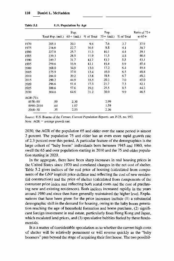
The gross demographics of the U.S. population are responsible for much of the strain on the housing market and are also an important factor in the evolu- tion of housing costs. Table 5.1 gives population statistics through 1985 and “middle-series” projections of the U.S. Bureau of the Census through 2030. The percentage of the population age 65 and older has risen sharply since 1970 and will continue to rise rapidly for the next forty years. While the annual growth rate (AGR) of the total population is less than 1 percent from 1970 to

Daniel L. McFadden is professor of economics at the University of California, Berkeley, and a research associate of the National Bureau of Economic Research.

This research was supported by a grant from the National Institute on Aging to the National Bureau of Economic Research. Chunrong Ai provided research assistance. Miki Seko provided much of the data for comparisons of the United States and Japan.

109

110 Daniel L. McFadden

Table 5.1 U.S. Population by Age ~~ ~

Pop. Pop. Ratio of 75+ Total Pop. (mil.) 65+ (mil.) % of Total 75+ (mil.) % of Total to 65+

1970 1975 1980 1985 1990 1995 2000 2005 2010 2015 2020 2025 2030

AGR (%): 1970-90 1990-20 10 20 10-30

205.1 216.0 227.8 239.3 249.7 259.6 268.0 275.9 284.0 290.2 296.6 300.6 304.6

.99

.64

.35

20.1 22.7 25.7 28.5 31.7 33.9 34.9 37.0 39.2 44.9 51.4 57.6 64.6

2.30 1.07 2.53

9.8 7.6 10.5 8.8 11.3 10.1 11.9 11.5 12.7 13.7 13.1 15.4 13.0 17.2 13.4 18.0 13.8 18.8 15.5 20.2 17.3 21.7 19.2 25 .5 21.2 30.0

2.99 1 .59 2.36

3.7 4.1 4.4 4.8 5.5 5.9 6.4 6.5 6.7 7.0 7.3 8.5 9.9

37.9 38.7 39.1 40.4 43.1 45.4 49.4 48.8 48.2 45.0 42. I 44.2 46.5

~ ~~ ~~ ~

Source: U.S. Bureau of the Census, Current Population Reports, ser. P-25, no. 952. Note: AGR = average growth rate.

2030, the AGR of the population 65 and older over the same period is almost 2 percent. The population 75 and older has an even more rapid growth rate of 2.3 percent over this period. A particular feature of the demographics is the large cohort of “baby boom” individuals born between 1945 and 1960, who swell the 65 and over population starting in 2010 and the 75 and older population starting in 2020.

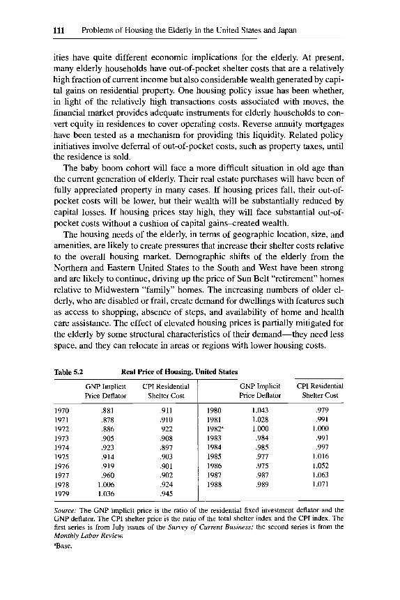
In the aggregate, there have been sharp increases in real housing prices in the United States since 1970 and correlated changes in the net cost of shelter. Table 5.2 gives indices of the real price of housing (calculated from components of the GNP implicit price deflator and reflecting the cost of new residential construction) and the price of shelter (calculated from components of the consumer price index and reflecting both rental costs and the cost of purchas- ing new and existing residences). Both indices increased rapidly in the years around 1980 and since then have generally maintained the higher level. Expla- nations that have been given for the price increases include ( 1 ) a substantial demographic shift in the demand for housing, owing to the baby boom generation reaching the age of household formation and home purchase, (2) significant foreign investment in real estate, particularly from Hong Kong and Japan, which escalated land prices, and (3) speculative bubbles fueled by these funda- mentals.

It is a matter of considerable speculation as to whether the current high costs of shelter will be relatively permanent or will reverse quickly as the “baby boomers” pass beyond the stage of acquiring their first house. The two possibil-

111 Problems of Housing the Elderly in the United States and Japan

ities have quite different economic implications for the elderly. At present, many elderly households have out-of-pocket shelter costs that are a relatively high fraction of current income but also considerable wealth generated by capital gains on residential property. One housing policy issue has been whether, in light of the relatively high transactions costs associated with moves, the financial market provides adequate instruments for elderly households to convert equity in residences to cover operating costs. Reverse annuity mortgages have been tested as a mechanism for providing this liquidity. Related policy initiatives involve deferral of out-of-pocket costs, such as property taxes, until the residence is sold.

The baby boom cohort will face a more difficult situation in old age than the current generation of elderly. Their real estate purchases will have been of fully appreciated property in many cases. If housing prices fall, their out-of- pocket costs will be lower, but their wealth will be substantially reduced by capital losses. If housing prices stay high, they will face substantial out-of- pocket costs without a cushion of capital gainsxreated wealth.

The housing needs of the elderly, in terms of geographic location, size, and amenities, are likely to create pressures that increase their shelter costs relative to the overall housing market. Demographic shifts of the elderly from the Northern and Eastern United States to the South and West have been strong and are likely to continue, driving up the price of Sun Belt “retirement” homes relative to Midwestern “family” homes. The increasing numbers of older elderly, who are disabled or frail, create demand for dwellings with features such as access to shopping, absence of steps, and availability of home and health care assistance. The effect of elevated housing prices is partially mitigated for the elderly by some structural characteristics of their demand-they need less space, and they can relocate in areas or regions with lower housing costs.

Table 5.2 Real Price of Housing, United States

~

1970 1971 1972 1973 1974 1975 1976 1977 1978 1979

GNP Implicit CPI Residential GNP Implicit CPI Residential Price Deflator Shelter Cost Price Deflator Shelter Cost

381 378 286 ,905 ,923 ,914 .919 ,960

1.006 1.036

,911 .910 922 ,908 ,897 ,903 ,901 ,902 ,924 ,945

1980 1.043 1981 1.028 1982” 1.000 1983 ,984 1984 .985 1985 .977 1986 ,975 1987 ,987 1988 ,989

,979 ,991

1.000 .99 1 ,997

1.016 1.052 1.063 I .07 1

Source: The GNP implicit price is the ratio of the residential fixed investment deflator and the GNP deflator. The CPI shelter price is the ratio of the total shelter index and the CPI index. The first series is from July issues of the Survey of Current Business; the second series is from the Monthly Labor Review. “Base.


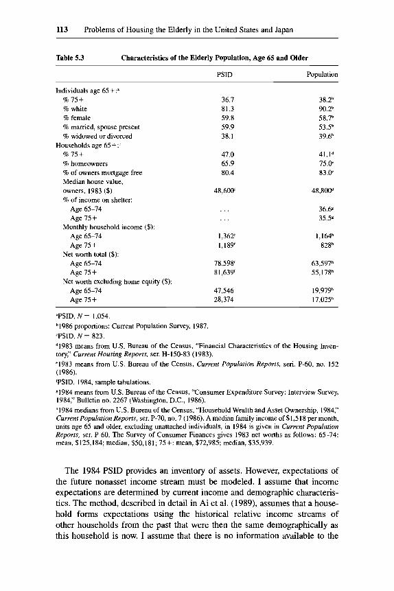
The information in this paper on the housing and economic status of the elderly is drawn primarily from the 1984 wave of the Panel Study on Income Dynamics (PSID). This panel was started in 1968 with approximately 5,000 households and has since interviewed these and split-off households annually. My analysis is based on 2,089 households that had a household member aged 35 or older in 1968. Of these, 960 had a household member aged 50 or older, and 193 had a member aged 65 or older, in 1968. The original panel oversampled the poor and minorities. Table 5.3 describes some of the demographic features of the PSID sample, with U.S. population statistics shown for comparison. The effects of oversampling the poor and minorities are minor, and the panel appears to be fairly representative of U.S. households.

Section 5.1 of this paper outlines the methodology used to measure wealth and shelter costs, taking into account the contribution of transactions costs and the rather complex system of tax entitlements and offsets enjoyed by homeowners in the United States. Section 5.2 summarizes information on aggregate holdings of various assets by the elderly; sections 5.3 and 5.4 discuss the distribution of these holdings. Section 5.5 provides information on user costs and the distribution of shelter burdens that they imply for elderly households. Sec- tion 5.6 gives data on features of the dwellings occupied by the elderly and discusses mobility. Section 5.7 examines the effects on user costs and shelter burdens of several of the tax policies that have been adopted, or are under discussion, in the United States, Section 5.8 compares the housing problems of U.S. and Japanese elderly along several dimensions. Section 5.9 concludes.

5.1 Household Wealth and Shelter Costs: Methodology

An initial picture of the economic and housing status of the elderly can be obtained from statistics on current income and assets, out-of-pocket housing costs, and physical characteristics of dwellings. I summarize some of these statistics, from government sources and from the PSID. Going beyond these statistics, I try to account for the effects on economic well-being of mobility with its associated transactions costs, tax treatment of home ownership, and expectations about mortality, health, income, and housing out-of-pocket costs.

5.1.1 Income and Wealth

First consider the wealth of elderly households. This will include not only the net worth of current real and financial assets but also the expected present value of the future stream of non-asset-generated income (i.e., labor income, Social Security and other transfers, and employer-provided pension income). To account for differences in life expectancy across households and differences in expected present value of nonasset income expectations, I convert assets and the nonasset income stream into life annuities.'

1. For a couple, a double life annuity is calculated that provides a flat income stream as long as one of the two individuals survives.


Table 5.3 Characteristics of the Elderly Population, Age 65 and Older

PSID Population

Individuals age 65 + := % 75+ % white % female % married, spouse present % widowed or divorced

% 75+ % homeowners % of owners mortgage free Median house value, owners, 1983 ($) % of income on shelter:

Age 65-74 Age 75 +

Age 65-74 Age 75 i

Age 65-74 Age 75+

Age 65-74 Age 75 +

Households age 65 + :c

Monthly household income ($):

Net worth total ($):

Net worth excluding home equity ($):

36.7 81.3 59.8 59.9 38.1

47.0 65.9 80.4

48,600‘

1,362‘ 1,189‘

78,598‘ 81.639‘

47,546 28,374

41.1d 75.w 83.P

48,800d

36.69 35.59

1,164h 82gh

’PSID, N = 1,054. h1986 proportions: Current Population Survey, 1987. ‘PSID, N = 823. d1983 means from U.S. Bureau of the Census, “Financial Characteristics of the Housing Inven- tory,’’ Current Housing Reports, ser. H-150-83 (1983). ‘1983 means from US. Bureau of the Census, Currenr Population Reports, seri. P-60, no. 152 (1986). TSID, 1984, sample tabulations. ~ 1 9 8 4 means from U.S. Bureau of the Census, “Consumer Expenditure Survey: Interview Survey, 1984:’ Bulletin no. 2267 (Washington, D.C., 1986). ”984 medians from U.S. Bureau of the Census, “Household Wealth and Asset Ownership, 1984,” Currenr Population Reports, ser. P-70, no. 7 (1986). A median family income of $1,518 per month, units age 65 and older, excluding unattached individuals, in 1984 is given in Currenr Population Reports, ser. P-60. The Survey of Consumer Finances gives 1983 net worths as follows: 65-74: mean, $125,184; median, $50,181; 75+: mean, $72,985; median, $35,939.

The 1984 PSID provides an inventory of assets. However, expectations of the future nonasset income stream must be modeled. I assume that income expectations are determined by current income and demographic characteristics. The method, described in detail in Ai et al. (1989), assumes that a household forms expectations using the historical relative income streams of other households from the past that were then the same demographically as this household is now. I assume that there is no information available to the


household that is not available to the econometrician, that there were no macro shocks through the period of the PSID panel that make the life-cycle income patterns observed therein unrepresentative, and that relative income expectations are stationary once trends are accounted for. Then, the ex post distribution of relative incomes for older households in the PSID coincides with the ex ante expectation of younger households. I estimate this ex post distribution for total income and for income components: labor, transfer, and nonasset.

The income profiles starting from year t with a head of age A, are assumed to have the form

where s = 1, 2, . . . denotes future years, the 0, are coefficients, and the d,(A) form a quadratic spline that permits a flexible description of the life-cycle income profile. This system is log-linear in parameters and is estimated using PSID data stacked by household, and by year within household, conditioned on all income variables appearing in the regression being positive. The cases of zero income almost all correspond to nonsurvival, and for these the regression conditioning corresponds to the conditional forecast needed.

This formulation of the life-cycle income profile and estimation method dif- fers from more common autoregressive forecasting models in that I use a direct s-period-ahead forecast rather than an s-step-ahead iterative forecast. The reason I do this is that I anticipate the existence of persistent individual effects, which can be approximated in an autoregressive model only with a lengthy lag. A second variation on conventional analysis is that I combine labor and pension income and do not condition on retirement. Thus, this model gives unconditional income profiles that incorporate sample information on retirement patterns and their interdependence on earnings and pension profiles. This approach circumvents the necessity of specifying a correct structural model of the retirement process and is robust to the nature of this structure. One draw- back is that I am unable to do policy analysis of housing behavior response to structural changes in retirement programs or to forecast housing demand in a future where structural changes in retirement programs have occurred.

Income forecasts from the model are conditioned only on initial household demographics, not on survival of individual household members. Thus, they incorporate the expected effect on income on nonsurvival of head or spouse. This avoids structural modeling of, say, income conditioned on the event of future widowhood. However, in order to estimate the model using the eleven- year window from 1974 through 1984 in which the PSID has consistent income data and associated demographics, I assume that households treat their initial demographic state as time invariant. For example, a household con- sisting of a couple with head aged 60 is postulated to assume that changes in its income profile between age 80 and age 90 will resemble the changes over a decade of couples that start with head age 80. In fact, there is a substantial


probability that this head will die before age 80, and the household’s income profile in this future decade will more closely resemble that of widows that start at age 80. Hence my assumption is not very satisfactory. A better solution would be to use data on full life cycles in which future income profiles could be constructed conditioned on demographic status at each age.

5.1.2 Net Shelter Costs

The first component in a calculation of the expected present value of user cost of housing is a stream of out-of-pocket costs that will be incurred as long as the current dwelling is occupied. For renters, this is simply rent plus utilities. In a few states, there is some state income-tax offset for rental expenses. For homeowners, the out-of-pocket costs include mortgage payments, real estate taxes, utilities, maintenance, and insurance. The deductibility of homeowner interest and real estate tax expenses in federal income taxes, and some state income taxes, is an important offsetting factor in calculating out-of-pocket expenses.

The second major element in user cost is the transaction cost associated with moves, purchases, or sales. A house purchase involves loan fees, title insurance, and other closing costs. A sale involves real estate broker’s fees. Moving between dwellings involves direct moving expenses, less easily measured time and money costs in setting up the household, and psychic costs of disruption.

A third component in user cost for owners is capital gains on the housing asset. An increase in the present value of net equity resulting from sale of a home at a future date, rather than immediately, is an additional component that offsets the cost of ownership. Calculation of capital gains is complicated by their tax treatment, particularly a one-time exemption for elderly households that was in effect during the period of this study. A second complication arises in the treatment of homes sold as part of the household’s estate after the death of the household. In this analysis, I take the “Ricardian equivalence” view that bequests, including home equity, have utility to the household and are determined jointly with lifetime consumption. With further simplifications, this leads me to treat capital gains from sale of a house symmetrically whether the household is living or not. Alternatively, the household may treat bequests as the unintended residual of a “self-insured annuity” that contributes little to utility. This would increase the perceived cost of options in which the household owns its home until death, at least to the extent that increases in home equity are not offset dollar for dollar by decreases in liquid assets.

In calculating the present value of expected user cost of housing, important factors will be the discount rate that the consumer uses, the length of time the household stays in the current dwelling, and the likely transitions after the household leaves the current dwelling. First, the Fisherian consumer in an im- perfect capital market will use a discount rate that depends endogenously on lending or borrowing status, credit limits, and instruments available in each period. The length of time the household stays in the dwelling will be influ-


enced by largely exogenous factors such as the death of one or more household members, job changes or retirements, and changes in health status (i.e., ability to live unaided in a dwelling with specific characteristics). It will also be influ- enced by endogenous response to factors such as realized cost of current dwelling and alternatives and life-cycle issues involving current income, portfolio of assets including equity in owner-occupied housing, and bequest motives.

The approach taken in this paper is to calculate an annualized expected present value of user cost taking all the factors above into account, in a fashion that mimics the calculations of a representative household. However, the endogenous interactions between life-cycle income and consumption patters that enter the discount rate, and the endogenous decisions of length of stay that would enter the actual calculation of a consumer that solves a life-cycle dynamic sto- chastic program, are replaced by exogenous rates and probabilities based on statistical averages from a population of similarly situated individuals.

The formula that I use for calculating user cost of housing is simply the value of a life annuity that has the same expected present value as the actual stream of housing costs, including capital gains and losses on transactions during the household’s lifetime, and including capital gains and losses from liqui- dation of the housing component of bequests on the death of the household. In this formula, future costs are discounted at a rate reflecting the market interest rate and the household’s survival probability. I consider discrete choice among three dwelling sizes, as well as tenure, so that in each year the household has the alternative of not moving or of moving to one of the six possible sizekenure combinations. I incorporate a relatively complete model of the offsets resulting from federal and state treatment of property taxes, mortgage interest, and capital gains. I incorporate concrete models of expectations about future incomes, price levels, interest rates, and mobility. These models assume that households are Bayesian “imitators” who use the experiences of similarly situated households in the past to forecast the distribution of their own responses in the future. I note that these are not necessarily “rational expectations,” nor in the implementation are they based solely on information available prior to the de- cision year.

5.2 Income and Wealth

Households in the United States enter the “postretirement” phase of their life cycle facing future income streams that are sharply lower than their life- cycle peak. Social Security income, private pensions, and public assistance programs are, however, sufficient to assure that most elderly households are not in poverty. For many households, owner-occupied housing is the only major asset. Asset holdings decline with age, but not as rapidly as life-cycle theo- ries without strong bequest motives would suggest.

The money income of households, classified by age, is shown in table 5.4. Income levels for those over age 65 are less than 60 percent of income levels


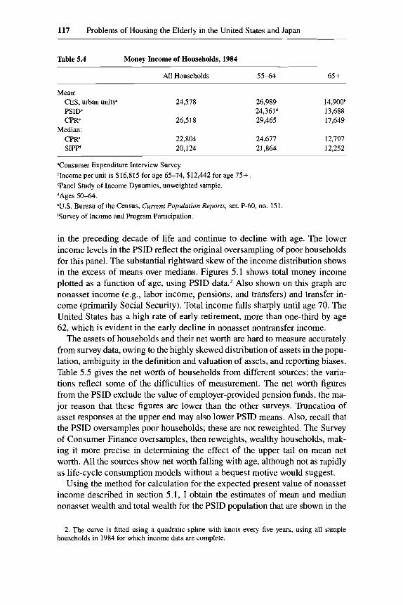
Table 5.4 Money Income of Households, 1984

All Households 55-64 65 +

Mean: CES, urban unitsa 24,578 PSIDc CPR’ 26,5 18

Median: CPR’ 22,804 SIPP‘ 20,124

26,989 14,900b 24,361d 13,688 29,465 17,649

24,677 12,797 21,864 12,252

“Consumer Expenditure Interview Survey. bIncome per unit is $16.815 for age 65-74, $12,442 for age 75+. ‘Panel Study of Income Dynamics, unweighted sample. dAges 50-64. W.S. Bureau of the Census, Current Population Reports, ser. P-60, no. 151. ‘Survey of Income and Program Participation.

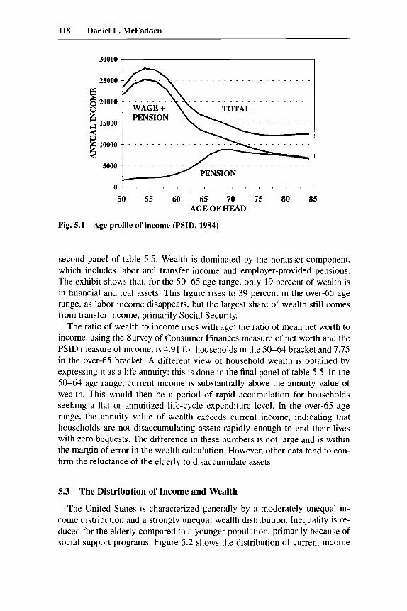
in the preceding decade of life and continue to decline with age. The lower income levels in the PSID reflect the original oversampling of poor households for this panel. The substantial rightward skew of the income distribution shows in the excess of means over medians. Figures 5.1 shows total money income plotted as a function of age, using PSID data.2 Also shown on this graph are nonasset income (e.g., labor income, pensions, and transfers) and transfer income (primarily Social Security). Total income falls sharply until age 70. The United States has a high rate of early retirement, more than one-third by age 62, which is evident in the early decline in nonasset nontransfer income.

The assets of households and their net worth are hard to measure accurately from survey data, owing to the highly skewed distribution of assets in the population, ambiguity in the definition and valuation of assets, and reporting biases. Table 5.5 gives the net worth of households from different sources; the varia- tions reflect some of the difficulties of measurement. The net worth figures from the PSID exclude the value of employer-provided pension funds, the major reason that these figures are lower than the other surveys. Truncation of asset responses at the upper end may also lower PSID means. Also, recall that the PSID oversamples poor households; these are not reweighted. The Survey of Consumer Finance oversamples, then reweights, wealthy households, making it more precise in determining the effect of the upper tail on mean net worth. All the sources show net worth falling with age, although not as rapidly as life-cycle consumption models without a bequest motive would suggest.

Using the method for calculation for the expected present value of nonasset income described in section 5.1, I obtain the estimates of mean and median nonasset wealth and total wealth for the PSID population that are shown in the

2. The curve is fitted using a quadratic spline with knots every five years, using all sample households in 1984 for which income data are complete.


30000 I

25000

8 20000

z 15000

d 9 10000

4 5000

WAGE + TOTAL PENSION

/ PENSION

50 55 60 65 70 75 80 85 AGE OF HEAD

Fig. 5.1 Age profile of income (PSID, 1984)

second panel of table 5.5. Wealth is dominated by the nonasset component, which includes labor and transfer income and employer-provided pensions. The exhibit shows that, for the 50-65 age range, only 19 percent of wealth is in financial and real assets. This figure rises to 39 percent in the over-65 age range, as labor income disappears, but the largest share of wealth still comes from transfer income, primarily Social Security.

The ratio of wealth to income rises with age: the ratio of mean net worth to income, using the Survey of Consumer Finances measure of net worth and the PSID measure of income, is 4.91 for households in the 50-64 bracket and 7.75 in the over-65 bracket. A different view of household wealth is obtained by expressing it as a life annuity; this is done in the final panel of table 5.5. In the 50-64 age range, current income is substantially above the annuity value of wealth. This would then be a period of rapid accumulation for households seeking a flat or annuitized life-cycle expenditure level. In the over-65 age range, the annuity value of wealth exceeds current income, indicating that households are not disaccumulating assets rapidly enough to end their lives with zero bequests. The difference in these numbers is not large and is within the margin of error in the wealth calculation. However, other data tend to con- firm the reluctance of the elderly to disaccumulate assets.

5.3 The Distribution of Income and Wealth

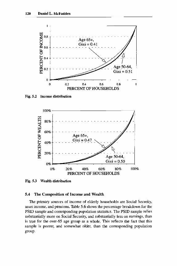
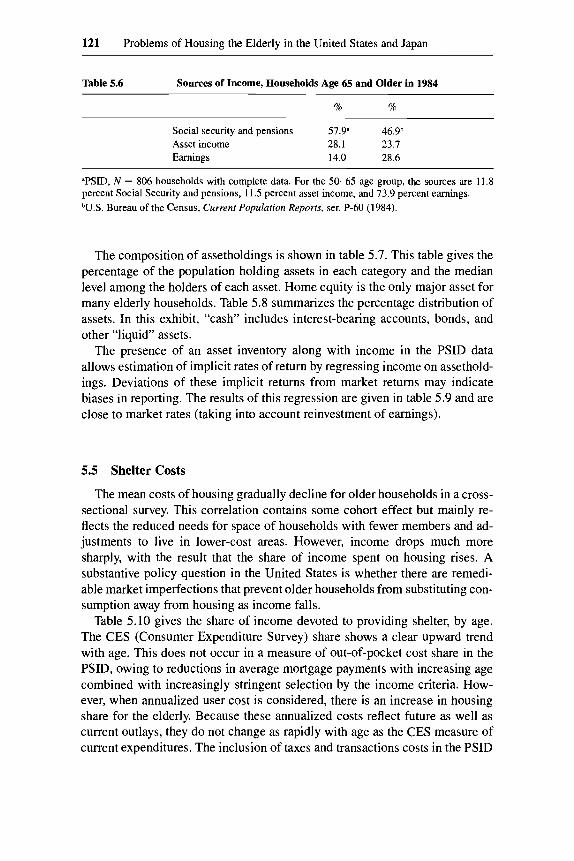
The United States is characterized generally by a moderately unequal income distribution and a strongly unequal wealth distribution. Inequality is reduced for the elderly compared to a younger population, primarily because of social support programs. Figure 5.2 shows the distribution of current income


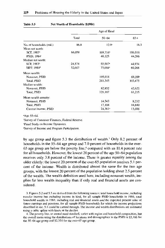
Table 5.5 Net Worth of Households ($1984)

Age of Head ~~~

Total 50-64 65 +

No. of households (mil.) Mean net worth:

SCF, 1983b PSID, 1984'

Median net worth: SCF, 1983b SIPP, 1984"

Mean wealth: Nonasset, PSID Total, PSID

Median wealth: Nonasset, PSID Total, PSID

Mean wealth annuity: Nonasset, PSID Total, PSID Current income, PSID

86.8 12.9"

66.050 119,714" 46,325

24,574 55,587" 32,667 73,664

195,018 241,343

82,852 121.167

14,543 17,104 24,361"

18.3

106,O 16 44,266

44,934 60,266

69,209 113,475

42,622 61.215

8,232 14,840 13,688

"Age 55-64. bSurvey of Consumer Finances, Federal Reserve 'Panel Study on Income Dynamics. "Survey of Income and Program Participation.

by age group and figure 5.3 the distribution of ~ e a l t h . ~ Only 8.2 percent of households in the 55-64 age group and 7.0 percent of households in the over- 65 age group are below the poverty line: compared with an 11.4 percent rate for all households. However, the lowest 20 percent of the age 50-64 population receives only 3.8 percent of the income. There is greater equality among the older elderly: the lowest 20 percent of the over-65 population receives 5.1 percent of the income. Wealth is distributed almost the same for the two age groups, with the lowest 20 percent of the population holding about 2.5 percent of the wealth. The wealth definition used here, including nonasset wealth, im- plies far less wealth inequality than if only real and financial assets are considered.

3. Figures 5.2 and 5.3 are derived from the following sources: total household income, including transfer income but excluding income in kind, for all sample PSLD households in 1984; total household wealth in 1984, including real and financial assets and the expected present value of future earnings and pensions, for all sample PSID households for which the income projections described in sec. 5.1 could be carried through. The income and wealth distributions are estimated using a cubic spline with knots at the deciles.

4. The poverty line, or annual need standard, varies with region and household composition, but the overall mean using the distributions of locations and demographics in the PSID is $3,166 for the 50-64 age group and $2,354 for the over-65 age group.


w 2 0.8

8 0.6 8 8

0.4 w U 2 0.2

0

Age 65+, Gini = 0.41

_ _ . . . . . . .

0 0.2 0.4 0.6 0.8

PERCENT OF HOUSEHOLDS

Fig. 5.2 Income distribution

100% ,

1

80%

$ 60%

8

8 40%

z 20%

0% Gini = 0.50

0% 20% 40% 60% 80% 100% PERCENT OF HOUSEHOLDS

Fig. 5.3 Wealth distribution

5.4 The Composition of Income and Wealth

The primary sources of income of elderly households are Social Security, asset income, and pensions. Table 5.6 shows the percentage breakdown for the PSID sample and corresponding population statistics. The PSID sample relies substantially more on Social Security, and substantially less on earnings, than is true for the over-65 age group as a whole. This reflects the fact that this sample is poorer, and somewhat older, than the corresponding population group.


Table 5.6 Sources of Income, Households Age 65 and Older in 1984

% %

Social security and pensions 5 7 9 46.9b Asset income 28.1 23.7 Earnings 14.0 28.6

“PSID, N = 806 households with complete data. For the 50-65 age group, the sources are 11.8 percent Social Security and pensions, 11.5 percent asset income, and 73.9 percent earnings. bU.S. Bureau of the Census, Current Popularion Reports, ser. P-60 (1984).

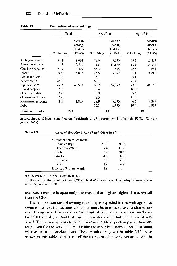
The composition of assetholdings is shown in table 5.7. This table gives the percentage of the population holding assets in each category and the median level among the holders of each asset. Home equity is the only major asset for many elderly households. Table 5.8 summarizes the percentage distribution of assets. In this exhibit, “cash” includes interest-bearing accounts, bonds, and other “liquid” assets.

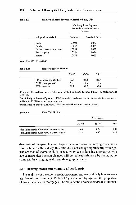
The presence of an asset inventory along with income in the PSID data allows estimation of implicit rates of return by regressing income on assetholdings. Deviations of these implicit returns from market returns may indicate biases in reporting. The results of this regression are given in table 5.9 and are close to market rates (taking into account reinvestment of earnings).

5.5 Shelter Costs

The mean costs of housing gradually decline for older households in a cross- sectional survey. This correlation contains some cohort effect but mainly reflects the reduced needs for space of households with fewer members and adjustments to live in lower-cost areas. However, income drops much more sharply, with the result that the share of income spent on housing rises. A substantive policy question in the United States is whether there are remedi- able market imperfections that prevent older households from substituting consumption away from housing as income falls.

Table 5.10 gives the share of income devoted to providing shelter, by age. The CES (Consumer Expenditure Survey) share shows a clear upward trend with age. This does not occur in a measure of out-of-pocket cost share in the PSID, owing to reductions in average mortgage payments with increasing age combined with increasingly stringent selection by the income criteria. How- ever, when annualized user cost is considered, there is an increase in housing share for the elderly. Because these annualized costs reflect future as well as current outlays, they do not change as rapidly with age as the CES measure of current expenditures. The inclusion of taxes and transactions costs in the PSID


Table 5.7 Composition of Assetholdings

Total Age 55-64 Age 65+

Median Median Median among among among

Holders Holders Holders % Holding (1984$) % Holding (1984$) % Holding (1984$)

Savings accounts Bonds, insurance Checking accounts Stocks Business assets Automobiles Equity in home Rental property Other real estate Government bonds Retirement accounts Debt

71.8 3,066 8.5 9.47 1

53.9 449 20.0 3,892 12.8 85.8 64.3 40,597 9.5

10.0 15.0 19.5 4,805

Households (mil.) 86.8

76.0 7,340 11.5 13,559 55.4 568 25.5 5,662 15.1 89.1 80.2 54,059 15.4 15.9 18.3 38.9 6,390 37.3 2,350

12.9

77.5 13,255 11.6 18,144 48.5 65 1 21.1 6,882 5.1

71.4 73.0 46,192 10.8 8.4

11.3 6.5 6,369

19.0 1,987

18.2

Source: Survey of Income and Program Participation, 1984, except debt data from the PSID, 1984 (age group 50-65).

Table 5.8 Assets of Household Age 65 and Older in 1984

% distribution of net worth: Home equity 50.3” 38.6h Other real estate 7.4 11.2 Cash 33.2 30.3 Stocks 4.1 8.6 Business 3.1 4.5 Other 1.9 6.8

Debt as a % of net worth 1.9 . . .

“PSID, 1984, N = 693 with complete data. b1984 data, U.S. Bureau of the Census, “Household Wealth and Asset Ownership,” Current Popu- lation Reports, ser. P-70.

user cost measure is apparently the reason that it gives higher shares overall than the CES.

The relative user cost of owning to renting is expected to rise with age since owning involves transactions costs that must be amortized over a shorter period. Comparing these costs for dwellings of comparable size, averaged over the PSID sample, we find that this increase does occur but that it is relatively small. The reason appears to be that remaining life expectancy is sufficiently long, even for the very elderly, to make the amortized transactions cost small relative to out-of-pocket costs. These results are given in table 5.1 1 . Also shown in this table is the ratio of the user cost of moving versus staying in


Table 5.9 Relation of Asset Income to Assetholdings, 1984

Ordinary Least Squares Dependent Variable: Asset

Income

Independent Variable Estimate Standard Error

Cash .0504 .0029 Bonds .0257 ,0005 Business nonlabor income .0259 .0037 Real property ,025 1 ,0021 Stocks .0458 ,0025

Note: N = 823. R2 = 0.840.

Table 5.10 Shelter Share of Income

50-65 65-74 75 +

CES, shelter and utilities" 19.8 24.0 26.7 PSID out of pocketb 20.8 17.6 18.6 PSID user costC 27.1 33.7 33.4

~

Consumer Expenditure Survey, 1984, share of shelter plus utility expenditures. The first age group is 55-64. bPanel Study on Income Dynamics, 1982, annual expenditures for shelter and utilities, for households with $5,000 or more per year income. 'Panel Study on Income Dynamics, 1984, annualized user cost, median share.

Table 5.11 User Cost Ratios

Age Group

50-65 65-74 75 i

PSID, mean ratio of owner to renter user cost 1 1.45 1.54 1.58 PSID, mean ratio of mover to stayer user cost 1.17 1.17 1.14

dwellings of comparable size. Despite the amortization of moving costs over a shorter time for the elderly, this ratio does not change significantly with age. The absence of dramatic shifts in relative prices of housing alternatives with age suggests that housing changes will be induced primarily by changing income and by changing health and demographic status.

5.6 Housing Status and Mobility of the Elderly

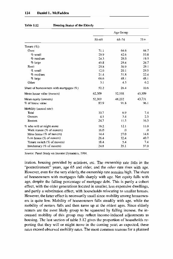
The majority of the elderly are homeowners, and many elderly homeowners are free of mortgage debt. Table 5.12 gives tenure by age and the proportion of homeowners with mortgages. The classification other includes institutional-


Table 5.12 Housing Status of the Elderly

Age Group

50-65 65-74 75 t

Tenure (%): Own:

8 small % medium % large

% small % medium % large

Rent:

Other

Share of homeowners with mortgages (%)

Mean house value (owners)

Mean equity (owners) % of house value

Mobility (annual rate): Total Owners Renters

% who will or might move Work reason (% of movers) More house (% of movers) Less house (% of movers) Tenure switch (% of movers) Involuntary (% of movers)

71.1 29.9 24.3 45.8 25.8 12.0 21.4 66.6

3.1

52.2

62,309

52,303 83.9

10.7 4.5

24.7

18.2 16.0 14.4 26.4 18.4 24.8

64.6 42.6 28.0 29.4 30.9 20.1 31.8 48.1

4.5

26.4

52,558

48,232 91.8

6.9 3.4

11.5

12.1 .o

27.0 32.4

5.4 35.1

64.7 53.8 19.5 26.7 29.1 29.5 22.4 48.1

6.2

10.6

45,509

43,73 1 96.1

7.4 2.3

16.3

11.0 .o

14.8 40.7

7.4 37.0

Source: Panel Study on Income Dynamics, 1984

ization, housing provided by relatives, etc. The ownership rate falls in the “postretirement” years, age 65 and older, and the other rate rises with age. However, even for the very elderly, the ownership rate remains high. The share of homeowners with mortgages falls sharply with age. Net equity falls with age, despite the falling percentage of mortgage debt. This is partly a cohort effect, with the older generations located in smaller, less expensive dwellings, and partly a substitution effect, with households relocating to smaller houses. However, the latter effect is necessarily small since mobility among homeowners is quite low. Mobility of homeowners falls steadily with age, while the mobility of renters falls and then turns up at the oldest ages. Since elderly renters are the most likely group to be squeezed by falling income, the increased mobility of this group may reflect income-induced adjustments to housing. The last section of table 5.12 gives the proportion of households reporting that they will or might move in the coming year; as expected, these rates exceed observed mobility rates. The most common reasons for a planned


move are to reduce dwelling size or cost (“less house”) or because of availability (“involuntary”). The last category includes units that become unavailable owing to demolition, condominium conversion, eviction, and so forth but, more important, also includes moves induced by health, divorce, or death of a household member. There are significant fractions of planned moves to increase dwelling size, even for the very old.

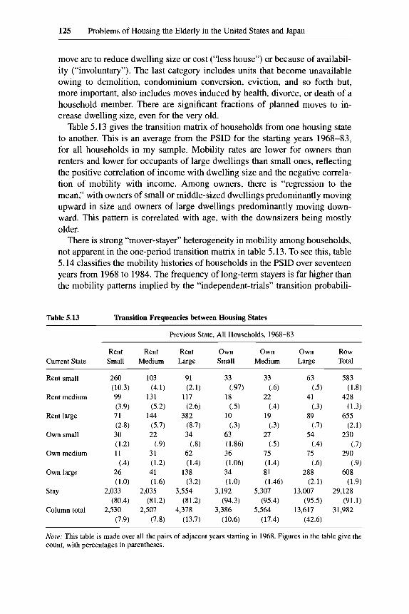
Table 5.13 gives the transition matrix of households from one housing state to another. This is an average from the PSID for the starting years 1968-83, for all households in my sample. Mobility rates are lower for owners than renters and lower for occupants of large dwellings than small ones, reflecting the positive correlation of income with dwelling size and the negative correlation of mobility with income. Among owners, there is “regression to the mean,” with owners of small or middle-sized dwellings predominantly moving upward in size and owners of large dwellings predominantly moving down- ward. This pattern is correlated with age, with the downsizers being mostly older.

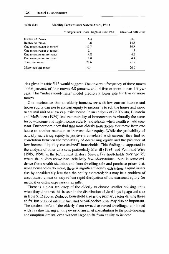
There is strong “mover-stayer” heterogeneity in mobility among households, not apparent in the one-period transition matrix in table 5.13. To see this, table 5.14 classifies the mobility histories of households in the PSID over seventeen years from 1968 to 1984. The frequency of long-term stayers is far higher than the mobility patterns implied by the “independent-trials” transition probabili-

Table 5.13 Transition Frequencies between Housing States

Previous State, All Households, 1968-83

Rent Rent Rent Own Own Own Row Current State Small Medium Large Small Medium Large Total

Rent small

Rent medium

Rent large

Own small

Own medium

Own large

Stay

Column total

260 (10.3) 99 (3.9) 71 (2.8) 30 ( 1 .2) 11

(.4) 26 ( 1 .O)

2,033 (80.4)

2,530 (7.9)

103

131 (5.2)

144

(5.7) 22

(.9) 31 ( 1 .2) 41 ( 1.6)

2,035 (81.2)

2,507

(4.1)

(7.8)

91 (2.1)

117 (2.6)

382 (8.7) 34 (4

62

138

3,554

4,378

(1.4)

(3.2)

(81.2)

(13.7)

33

18

10

63 (1 36) 36 ( 1.06) 34 ( 1 .O)

3,192 (94.3)

3,386 (10.6)

(.97)

(3)

(.3)

33

22

19

27

75

81 ( 1.46)

5,307

5,564

( 6

(.4)

(.3)

(.5)

( 1.4)

(95.4)

(17.4)

63

41

89

54

75

288

13,007

13,617

(.5)

(.3)

(.7)

(.4)

(.6)

(2.1)

(95.5)

(42.6)

583

428

655

230

290

608

29,128

3 1,982

(1.8)

(1.3)

(2.1 )

(.7)

(.9)

(1.9)

(91.1)

Note: This table is made over all the pairs of adjacent years starting in 1968. Figures in the table give the count, with percentages in parentheses.


Table 5.14 Mobility Patterns over Sixteen Years, PSID

“Independent Trials” Implied Rates (%) Observed Rates (%)

Owner, no moves Renter, no moves One move, owner to owner One move, owner to renter One move, renter to owner One move, renter to renter Total, one move

More than one move

4.3 .6

13.7 1.1 3.8 3.0

21.6

73.4

38.0 14.3 10.8

I .8 4.7 4.4

21.7

26.0

ties given in table 5.13 would suggest. The observed frequency of three moves is 6.6 percent, of four moves 4.0 percent, and of tive or more moves 4.9 percent. The “independent-trials’’ model predicts a lower rate for five or more moves.

One mechanism that an elderly homeowner with low current income and house equity can use to convert equity to income is to sell the house and move to a rental unit or a less expensive house. In an analysis of PSID data, Feinstein and McFadden (1989) find that mobility of homeowners is virtually the same for low-income and high-income elderly households when wealth is held constant. Furthermore, they find that most elderly households that move from one house to another maintain or increase their equity. While the probability of actually increasing equity is positively correlated with income, they find no correlation between the probability of decreasing equity and the presence of low-income “liquidity-constrained” households. This tinding is supported in the analysis of other data sets, particularly Merrill (1984) and Venti and Wise (1989, 1990) in the Retirement History Survey. For households over age 75, where the studies above have relatively few observations, there is some evidence from wealth statistics and from dwelling sale and purchase prices that, when households do move, there is significant equity extraction. Liquid assets rise by considerably less than the equity extracted; this may be a problem of asset measurement or may reflect rapid dissipation of the extracted equity for medical or estate expenses or as gifts.

There is a clear tendency of the elderly to choose smaller housing units when they do move; this is seen in the distribution of dwellings by age and size in table 5.12 above. Reduced household size is the primary factor driving these shifts, but reduced maintenance and out-of-pocket costs may also be important. The modest shifts of the elderly from owned to rented dwellings, combined with this downsizing among owners, are a net contribution to the post-housing consumption stream, even without large shifts from equity to income.


5.7 Tax Policy Effects

Analysis of the behavior of elderly households suggests that, despite a rising share of expenditures on housing with age, there does not appear to be exten- sive “bottled-up’’ demand for mechanisms that permit housing costs to be post- poned and charged against the household’s bequests. In addition to the evidence that mobility rates and equity adjustments are insensitive to liquidity squeezes, there is direct evidence from reverse annuity mortgage (RAM) ex- periments in the United States that, in most cases, elderly homeowners are not seeking transactions that increase current income or reduce current expenditures via wealth adjustment^.^ This behavior may simply be driven by bequest motives or by precautionary demand for assets to cover contingencies such as health catastrophes. A demographic factor is that the poorest households, most in need of mechanisms to augment current income, are mostly those without any home equity or other assets available for conversion. In addition, a psycho- logical mechanism may be at work. For most households, net worth from financial and real assets is small relative to the present value of transfer income and pensions and, when annuitized, would yield only a small increase in current income. Most market mechanisms for annuitization of assets also have a significant loading penalty. Thus, the annuity appears to be a poor harvest of hard-earned savings.

To assess the potential gain or loss to elderly households from some of the tax policies that have been considered in the United States, I examined housing costs under alternative conditions. The two policies that 1 consider are directed toward increasing U.S. government tax receipts; the question is the magnitude of their negative effect on the elderly. The first of these is the elimination of the deductibility of mortgage interest in the calculation of taxable income. The second is the elimination of the one-time capital gains exclusion for sales of residential property by elderly households; the existing tax law on capital gains is summarized in table 5.15.

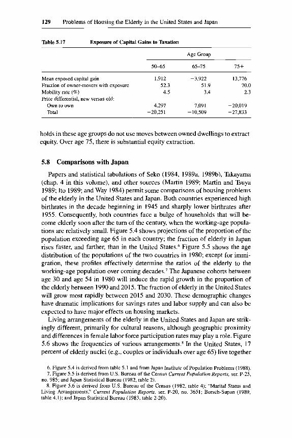
Table 5.16 shows the percentage change in the user costs of owners and renters when they choose to stay in their current dwelling in the coming year and when they consider moving to another rented or owned unit. The largest effect is on owner-stayers in the 50-65 age range, 3.4 percent, with a falling effect for older households who faced lower 1984 tax rates and had smaller mortgage balances. The effect on renter-stayers is not zero because the user cost calculation takes into account the probability of a future move to an owned dwelling.

The effects of eliminating the capital gains exclusion have been examined in detail by Newman and Reschovsky (1987), and I make only a summary calculation. The capital gains exclusion is relevant only for homeowners who

5 . In a RAM, the homeowner receives monthly income in exchange for a claim by the financial institution on the homeowner’s equity when the household dies and the estate is settled.


Table 5.15 Tax on Capital Gains from Resale of Residential Real Estate

Tax: 1974-80 198 1-84

Deduction: 1974-76

1977-78

1979-8 1 1982-84

0.5 X (capital gain) should be included in taxable income 0.4 X (capital gain) should be included in taxabale income

Person aged 65 or older can deduct any gains if adjusted selling price is not more than $20,000. Otherwise, he/she can deduct ($20,00O/selling price) X capital gain

Person aged 65 or older can deduct any gains if adjusted selling price is not more than $35,000. Otherwise, he/she can deduct ($35,00O/selling price) X capital gain

Person aged 55 or older can exclude $100,000 from capital gain Person aged 55 or older can exclude $125.000 from capital gain

Table 5.16 Effect on User Costs of Nondeductible Mortgage Interest

Age Group

50-65 65-75 75 +

Owners (%): Move to rental unit .o .o .o Move to owned unit I .6 1.2 .2 Stay 3.4 2.3 .5

Renters (%): Move to rental unit .O .o .o Move to owned unit .5 .2 .5 Stay .2 . I .o

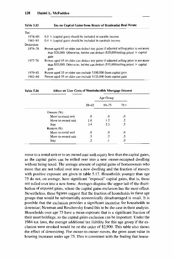
move to a rental unit or to an owned unit with equity less than the capital gains, as the capital gains can be rolled over into a new owner-occupied dwelling without being taxed. The average amount of capital gains of homeowners who move that are not rolled over into a new dwelling and the fraction of movers with positive exposure are given in table 5.17. Households younger than age 75 do not, on average, have significant “exposed” capital gains, that is, those not rolled over into a new home. Averages disguise the upper tail of the distribution of exposed gains, where the capital gains exclusion has the most effect. Nevertheless, these figures suggest that the fraction of households in these age groups that would be substantially economically disadvantaged is small. It is possible that the exclusion provides a significant incentive for households to downsize; Newman and Reschovsky found this to be the case in their analysis. Households over age 75 have a mean exposure that is a significant fraction of their asset holdings, so the capital gains exclusion can be important. Under the 1984 tax laws, the average additional tax liability for this age group if the exclusion were revoked would be on the order of $2,900. This table also shows the effect of downsizing. For owner-to-owner moves, the gross asset value in housing increases under age 75. This is consistent with the finding that house-


Table 5.17 Exposure of Capital Gains to Taxation

Age Group

50-65 65-75 75 +

Mean exposed capital gain 1,912 -3,922 13,776 Fraction of owner-movers with exposure 52.3 51.9 70.0 Mobility rate (96) 4.5 3.4 2.3 Price differential, new versus old:

Own to own 4,297 7,091 -20,019 Total -20,251 - 10,509 -27,833

holds in these age groups do not use moves between owned dwellings to extract equity. Over age 75, there is substantial equity extraction.

5.8 Comparisons with Japan

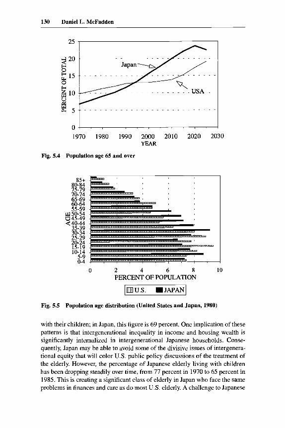
Papers and statistical tabulations of Seko (1984, 1989a, 1989b), Takayama (chap. 4 in this volume), and other sources (Martin 1989; Martin and Tsuya 1989; Ito 1989; and Way 1984) permit some comparisons of housing problems of the elderly in the United States and Japan. Both countries experienced high birthrates in the decade beginning in 1945 and sharply lower birthrates after 1955. Consequently, both countries face a bulge of households that will become elderly soon after the turn of the century, when the working-age populations are relatively small. Figure 5.4 shows projections of the proportion of the population exceeding age 65 in each country; the fraction of elderly in Japan rises faster, and farther, than in the United States.6 Figure 5.5 shows the age distribution of the populations of the two countries in 1980; except for immi- gration, these profiles effectively determine the ratios of the elderly to the working-age population over coming decades.’ The Japanese cohorts between age 30 and age 54 in 1980 will induce the rapid growth in the proportion of the elderly between 1990 and 201 5. The fraction of elderly in the United States will grow most rapidly between 2015 and 2030. These demographic changes have dramatic implications for savings rates and labor supply and can also be expected to have major effects on housing markets.

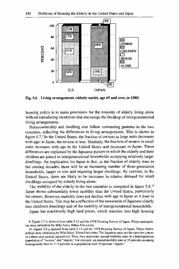
Living arrangements of the elderly in the United States and Japan are strik- ingly different, primarily for cultural reasons, although geographic proximity and differences in female labor force participation rates may play a role. Figure 5.6 shows the frequencies of various arrangements.8 In the United States, 17 percent of elderly nuclei (e.g., couples or individuals over age 65) live together

6. Figure 5.4 is derived from table 5.1 and from Japan Institute of Population Problems (1988). 7. Figure 5.5 is derived from U S . Bureau of the Census Current Population Reports, ser. P-25,

no. 985; and Japan Statistical Bureau (1982, table 2). 8. Figure 5.6 is derived from U.S. Bureau of the Census (1982, table 4); “Marital Status and

Living Arrangements,” Current Population Reports, ser. P-20, no. 365 1 ; Borsch-Supan (1989, table 4.1); and Japan Statistical Bureau (1983, table 2-20).


Fig. 5.5 Population age distribution (United States and Japan, 1980)

with their children; in Japan, this figure is 69 percent. One implication of these patterns is that intergenerational inequality in income and housing wealth is significantly internalized in intergenerational Japanese households. Conse- quently, Japan may be able to avoid some of the divisive issues of intergenerational equity that will color U.S. public policy discussions of the treatment of the elderly. However, the percentage of Japanese elderly living with children has been dropping steadily over time, from 77 percent in 1970 to 65 percent in 1985. This is creating a significant class of elderly in Japan who face the same problems in finances and care as do most U.S. elderly. A challenge to Japanese


100

80

60

40

20

0

U.S. JAPAN

Fig. 5.6 Living arrangements (elderly nuclei, age 65 and over, in 1980)

housing policy is to make provisions for the minority of elderly living alone without introducing incentives that encourage the breakup of intergenerational living arrangements.

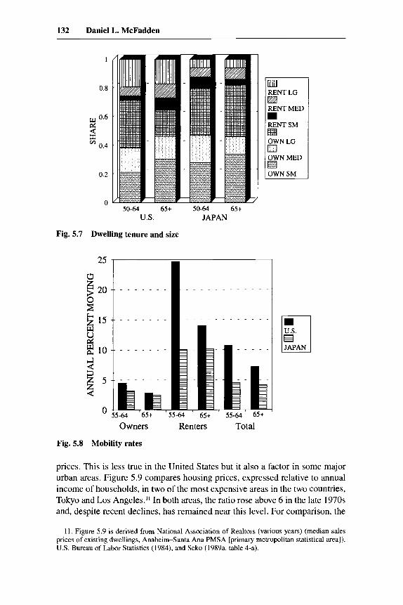
Homeownership and dwelling size follow contrasting patterns in the two countries, reflecting the differences in living arrangements. This is shown in figure 5.7.9 In the United States, the fraction of owners in large units decreases with age; in Japan, the reverse is true. Similarly, the fraction of renters in small units increases with age in the United States and decreases in Japan. These differences are explained by the Japanese pattern in which the elderly and their children are joined in intergenerational households occupying relatively larger dwellings. An implication for Japan is that, as the fraction of elderly rises in the coming decades, there will be an increasing number of three-generation households, larger in size and requiring larger dwellings. By contrast, in the United States, there are likely to be increases in relative demand for small dwellings occupied by elderly living alone.

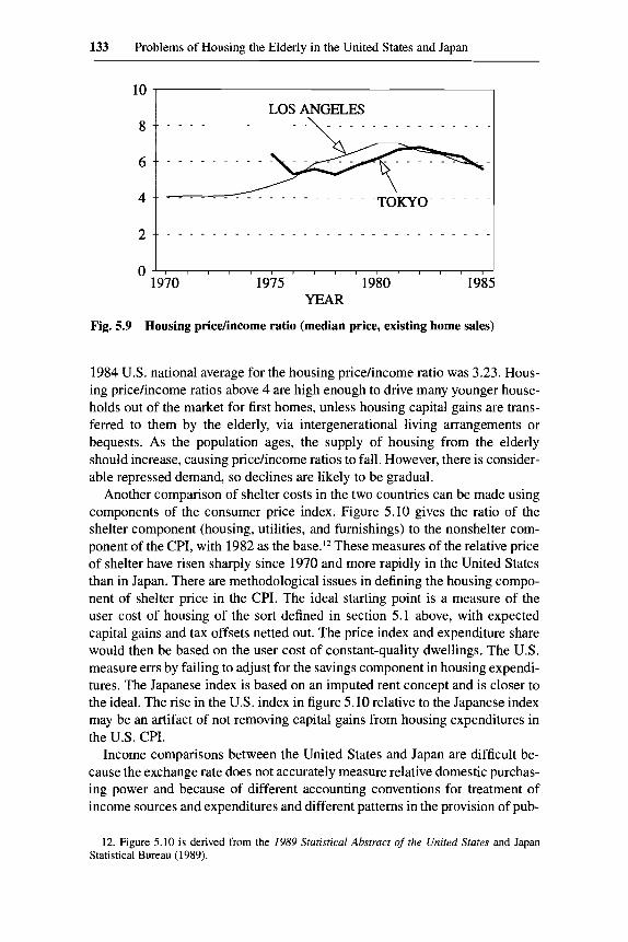
The mobility of the elderly in the two countries is compared in figure 5.8.1° Japan shows substantially lower mobility than the United States, particularly for renters. However, mobility does not decline with age in Japan as it does in the United States. This may be a reflection of the movement of Japanese elderly into children’s dwellings and of the mobility of intergenerational households.

Japan has notoriously high land prices, which translate into high housing

9. Figure 5.7 is derived from table 5.12 and the 1978 Housing Survey of Japan, Tokyo metropolitan area, tabulation by Miki Seko, Nihon University.

10. Figure 5.8 is derived from table 5.12 and the 1978 Housing Survey of Japan, Tokyo metropolitan area, tabulation by Miki Seko, Nihon University. The Japanese rates are the rates for a move in a three-year period, annualized. Thus, they understate annual mobility rates in a heterogeneous population of “movers” and “stayers.” For example, an annual mobility rate of 10 percent assuming homogeneity rises to 11.9 percent in a population with 50 percent “stayers.”


1

0.8

0.6

2 ' 0.4

0.2

0 50-64 65+ 50-64 65+

U.S. JAPAN

Fig. 5.7 Dwelling tenure and size

25

U

E !2 15 W u g 10

0 ' 65+ ' 55-64 ' 65+

E

Owners Renters Total

Fig. 5.8 Mobility rates

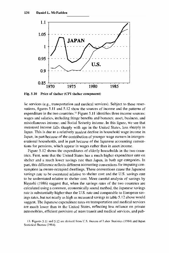
prices. This is less true in the United States but it also a factor in some major urban areas. Figure 5.9 compares housing prices, expressed relative to annual income of households, in two of the most expensive areas in the two countries, Tokyo and Los Angeles." In both areas, the ratio rose above 6 in the late 1970s and, despite recent declines, has remained near this level. For comparison, the

11. Figure 5.9 is derived from National Association of Realtors (various years) (median sales prices of existing dwellings, Anaheim-Santa Ana PMSA [primary metropolitan statistical area]), U.S. Bureau of Labor Statistics (1984), and Seko (1989a. table 4-a).


1984 U.S. national average for the housing pricehncome ratio was 3.23. Hous- ing pricehcome ratios above 4 are high enough to drive many younger households out of the market for first homes, unless housing capital gains are trans- ferred to them by the elderly, via intergenerational living arrangements or bequests. As the population ages, the supply of housing from the elderly should increase, causing pricehcome ratios to fall. However, there is considerable repressed demand, so declines are likely to be gradual.

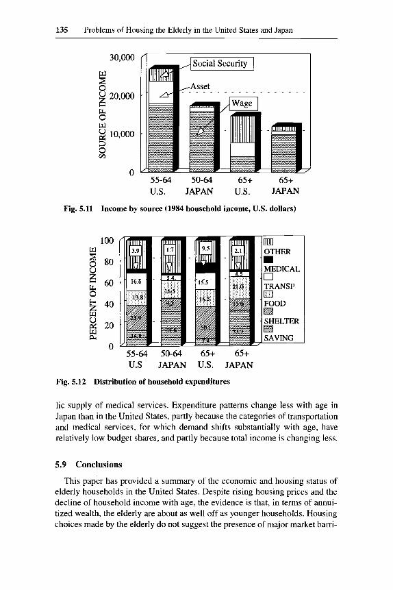
Another comparison of shelter costs in the two countries can be made using components of the consumer price index. Figure 5.10 gives the ratio of the shelter component (housing, utilities, and furnishings) to the nonshelter component of the CPI, with 1982 as the base.I2 These measures of the relative price of shelter have risen sharply since 1970 and more rapidly in the United States than in Japan. There are methodological issues in defining the housing component of shelter price in the CPI. The ideal starting point is a measure of the user cost of housing of the sort defined in section 5.1 above, with expected capital gains and tax offsets netted out. The price index and expenditure share would then be based on the user cost of constant-quality dwellings. The U.S. measure errs by failing to adjust for the savings component in housing expenditures. The Japanese index is based on an imputed rent concept and is closer to the ideal. The rise in the U.S. index in figure 5.10 relative to the Japanese index may be an artifact of not removing capital gains from housing expenditures in the U.S. CPI.

Income comparisons between the United States and Japan are difficult because the exchange rate does not accurately measure relative domestic purchas- ing power and because of different accounting conventions for treatment of income sources and expenditures and different patterns in the provision of pub-

12. Figure 5.10 is derived from the 1989 Statistical Abstract of the United States and Japan Statistical Bureau (1989).


1.1

1.05

1

0.95

0.9

1970 1975 1980 1985

Fig. 5.10 Price of shelter (CPI shelter component)

lic services (e.g., transportation and medical services). Subject to these reser- vations, figures 5.11 and 5.12 show the sources of income and the patterns of expenditure in the two ~0untries.I~ Figure 5.1 1 identities three income sources: wages and salaries, including fringe benetits and bonuses; asset, business, and miscellaneous income; and Social Security income. In this figure, we see that measured income falls sharply with age in the United States, less sharply in Japan. This is due to a relatively modest decline in household wage income in Japan, in part because of the contribution of younger wage earners in intergenerational households, and in part because of the Japanese accounting conventions for pensions, which appear in wages rather than in asset income.

Figure 5.12 shows the expenditures of elderly households in the two countries. First, note that the United States has a much higher expenditure rate on shelter and a much lower savings rate than Japan, in both age categories. In part, this difference reflects different accounting conventions for imputing consumption in owner-occupied dwellings. These conventions cause the Japanese savings rate to be overstated relative to shelter cost and the U.S. savings rate to be understated relative to shelter cost. More careful analysis of savings by Hayashi (1986) suggest that, when the savings rates of the two countries are calculated using a common, economically sound method, the Japanese savings rate is substantially higher than the U S . rate and comparable to European savings rates, but not nearly as high as measured savings in table 5.12 above would suggest. The Japanese expenditure rates on transportation and medical services are much lower than in the United States, reflecting less reliance on private automobiles, efficient provision of mass transit and medical services, and pub-

13. Figures 5.11 and 5.12 are derived from U S . Bureau of Labor Statistics (1984) and Japan Statistical Bureau (1984).


55-64 50-64 65+ 65+ U.S. JAPAN U.S. JAPAN

Fig. 5.11 Income by source (1984 household income, U.S. dollars)

100 w 8 80 U ’ 60

40 8

3 20 E W

0 55-64 50-64 65+ 65+ U.S JAPAN U.S. JAPAN

Fig. 5.12 Distribution of household expenditures

lic supply of medical services. Expenditure patterns change less with age in Japan than in the United States, partly because the categories of transportation and medical services, for which demand shifts substantially with age, have relatively low budget shares, and partly because total income is changing less.

5.9 Conclusions

This paper has provided a summary of the economic and housing status of elderly households in the United States. Despite rising housing prices and the decline of household income with age, the evidence is that, in terms of annuitized wealth, the elderly are about as well off as younger households. Housing choices made by the elderly do not suggest the presence of major market barri-


ers that prevent their making desired transactions between nonliquid and liquid assets. The demographics of the elderly population in the United States and the age distribution of capital gains from housing price increases suggest that the baby boom generation will face more difficult economic circumstances at the end of its life cycle than the previous generation. Japan faces a similar problem of an aging population, which may, however, have markedly different implications for the housing market, owing to the high incidence of intergenerational households that internalize some of the problems of economic equity between the young and the old.

References

Ai, C., J. Feinstein, D. McFadden, and H. Pollakowski. 1990. The dynamics of housing demand by the elderly: User cost effects. In Issues in the economics of aging, ed. D. Wise. Chicago: University of Chicago Press.

Borsch-Supan, A. 1989. Household dissolution and the choice of alternative living arrangements among elderly Americans. In The economics ofaging, ed. D. Wise. Chi- cago: Univesrity of Chicago Press.

Feinstein, J., and D. McFadden. 1989. The dynamics of housing demand by the elderly: 1. Wealth, cash-flow, and demographic effects. In The economics of aging, ed. D. Wise. Chicago: University of Chicago Press.

Hayashi, F. 1986. Why is Japan’s saving rate so apparently high? NBER Macroeconom- ics Annual, 000-000.

Ito, T. 1989. Housing bequests and saving in Japan. Working paper. Hitotsubashi Uni- versity.

Japan Institute of Population Problems. 1988. Latest demographic statistics, 1987. Tokyo: Ministry of Health and Welfare.

Japan Statistical Bureau. 1982. 1980population census of Japan. Vol. 2, Results of the first basic complete tabulation. Pt. 1, Whole Japan. Tokyo.

. 1983. Japan statistical yearbook. Tokyo.

. 1984. Annual report on the family income and expenditure survey, 1982.

. 1988. Annual report on the consumerprice index, 1988. Tokyo. Tokyo.

Martin, L. 1989. The graying of Japan. Population Bulletin 44: 1-40. Martin, L., and N. Tsuya. 1989. Interactions of middle-aged Japanese with their parents.

Merrill, S. 1984. Home equity and the elderly. In Retirement and economic behaviol;

National Association of Realtors. Various years. Existing home sales. Chicago. Newman, S., and J. Reschovsky. 1987. An evaluation of the one-time capital gains

Seko, M. 1984. Japanese homeownership: Relative tenure prices versus demographic

. 1989a. The effect of inflation on Japanese homeownership rates: Test of capital

. 1989b. Effects of subsidized home loans on housing decisions in Japan. Work-

Working paper. Honolulu: East-West Population Institute.

ed. H. Aaron and G. Burtless. Washington, D.C.: Brookings.

exclusion for older homeowners. AREUEA Journal 15:704-24.

factors. Nihon Daigaku Keizaikagakukenkyusho Kiyou 8:273-89.

market imperfections by time-series data. Working paper. Nihon University.

ing Paper. Nihon University.


US. Bureau of the Census. 1982. 1980 census of the population: Living arrangements ofthe children (PC80-2-4B). Washington, D.C.

U.S. Bureau of Labor Statistics. 1984. Consumer Expenditure Survey results, 1984. Bulletin no. 2267. Washington, D.C.

Venti, S., and D. Wise. 1989. Aging, moving, and housing wealth. In The economics of aging, ed. D. Wise. Chicago: University of Chicago Press.

. 1990. But they don’t want to reduce housing equity. In Issues in the economics of aging, ed. D. Wise. Chicago: University of Chicago Press.

Way, P. 1984. Issues and implications of the aging Japanese population. Staff Paper no. 6. Washington, D.C.: Center for International Research, U.S. Bureau of the Census.

This Page Intentionally Left Blank

Documents

Problems of Housing the Elderly in the United States and Japan · 5 Problems of Housing the Elderly in the United States and Japan Daniel L. McFadden The main issues in housing the