laurnal o/Mathematical Sciences, VoL 81, No. 2, 1996

P R O B L E M S OF T H E T H E O R Y OF B I T O P O L O G I C A L S P A C E S . 2

A. A. Ivanov UDC 515.122.4

This paper is the second part of a survey of recent results and new problems in the theory of bitopological spaces.

This paper and the next paper "Bibliography on bitopological spaces. 2" of the collection continue the papers [361] and [362] under the same titles. In total, these four papers should give rather a comprehensive idea of the development of the theory of bitopological spaces during the period untill 1990 including part of 1991, and of solved and up to now unsolved problems of this interesting, actively developing field of mathematics.

After publication of [361] and [362] in 1988, the author has received many reprints, preprints, and other information, which made his work easier. Valuable contribution to this was made by B. P. Dvalishvili, G. C, L. Bri~mmer, M. Cs V. Cs M. Mr~evi6, and I. L. Reilly. The author expresses to all of them his deepest gratitude.

Intending to continue publications on the problems of the theory of bitopological spaces and on the relevant literature, the author hopes that the circle of specialists cooperating with him in this field will broaden. Contact between the authors of the bitopological papers is quite necessary if only to coordinate the terms introduced and to straighten out, at last, the system of bitopological notions.

w 1. INTKODUCTION

The first part [358J of this work covers the period untill 1986 inclusive and part of 1987. The second part, which we present here, mainly concerns the papers published in 1987-1990. It also replenishes the gaps concerning earlier papers, and touches some papers published in 1991.

With few exceptions, we do not repeat here the contents of the first part. Thus, it is necessary to get acquainted with the basic notions and results of the theory of bitopological spaces by using other sources, preferably the first part itself.

All references are given according to "Bibliography ...," Nos. 1-245 of the first part and Nos. 246-478 of the second part.

The structure of this second part of the work "Problems of the theory of bitopological spaces" is, in general, parallel to the first one: it consists of the same five sections, and each of them can be considered as the continuation of the corresponding section of the first part. Thus, in w we consider further generalizations of the theory of topological spaces and related structures on the bitopological spaces in the sense of Kelly. In w we continue the presentation of the general theory of bitopological spaces. Sections 4 and 5 are devoted to the applications of the theory.

As before, the greater part of the bitopological literature is devoted to bitopological spaces (X, ~-1, r2) in the sense of Kelly, but general bitopological spaces (X, 8) begin to gradually at t ract the attention of a broader section of specialists. One can suppose that this tendency will persist and general bitopological spaces will become customary objects of study.

Nevertheless, w which is devoted to bitopotogical spaces in the sense of Kelly, is still a basic one. In general, its structure is similar to that of w of the first part: ten subsections continuing the corresponding subsections of w of the first part, and the new w devoted to fuzzy bitopological spaces,

In w we continue the construction of proper bitopological theory: new notions are introduced and their interconnections are studied.

The next two sections deal with the applications. In w we study bitopological representations of various classes of continuous mappings of topological spaces. In particular, we prove that some classes have no

Translated from Zapiski Nauchnykh Seminarov POMI, Vol. 208, 1993, pp. 5-67. Original article submitted June 18, 1993.

t072-3374/96/8102-2465515.00 o1996 Plenum Publishing Corporation 2465

bitopological representation, In w we continue the study o f bitopological manifolds and bitopological groups.

w 2. BITOPOLOGICAL SPACES IN TIIE SENSE OF KELLY

Starting the descriptive presentation of the classical theory of bitopological spaces, i.e., the theory of bitopological spaces in the sense of Kelly, first of all, we list the basic directions of study:

- separation axioms (subsections 1 and 3), - categorical methods (subsection 3), - connectedness (subsection 2), - compactness (subsection 4), - other special properties (subsection 5), - mappings (subsection 6), - extensions (subsection 7), - dimension (subsection 8), - connection with other structures (subsection 10), - fuzzy bitopological spaces (subsection 11). As in the first part of our survey, we try not only to give a more or less exact idea of the theory, but also

to critically discuss certain topics and to pose new problems.

2.1. S e p a r a t i o n ax ioms . The flow of papers devoted to transition of separation axioms from topological spaces to bitopological spaces in the sense of Kelly is gradually decreasing. In essence, there is nothing to generalize, since the old separation axioms already found a rather full reflection in bitopological literature and significantlly new separation axioms became a rarity. We shall discuss this situation somewhat later, but now we turn ourselves to the results of recent years.

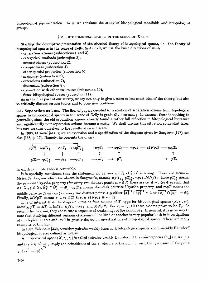
In 1986, Mr.%vi6 [414] gives an extension and a specification of the diagram given by Saegrove [197]; see also [358, p, 17]. Namely, he presents the diagram

wpT4 wpT3{ , wpT3 . , w ~ , wpT2 , wpT1 , rnpT1 , MNpT1 , mpTo

r T T r t T T pT4 ,.pT 3 �89 ~.pTz ,pT 2�89 , pT2 , pT1 , pTo

in which no implication is reversible. It is specially mentioned that the statement wp T4 , wp T3 of [197] is wrong. There are terms in

Mr~evi6's diagram which are absent in Saegrove's, namely wp T2�89 ,pT2t , rapT1, MNpT1 . Here pT2{ means the palrwise Urysohn property (for every two distinct points x, y E X there are G1 E rl , G2 E r2 such that x E GI,V E G2, O~ ~ f] 0'~ ~ = f~), wpT2{ means the weak pairwise Urysohn property, and rapT means the

middle pairwise Tl-axiom (for every two distinct points x, y either {z }~f] { - ~ = ~ or {x} r*f] { - ~ = ~). Finally, MNpT1 means T1 U 7"2 E T1 that is M N p T t -- sup 7"1.

It is of interest that the diagram contains four axioms of Tl-type for bitopological spaces (X, r l , v2), namely, pTl = biT1 =- infT1, wpTl, rapT1, and M N p T r . For ~-1 = ~-2, all these axioms prove to be 7'1. As seen in the diagram, they constitute a sequence of weakenings of the axiom pT1. In general, it is necessary to note that studying different versions of axioms of one kind or another is very popular both in investigations of topological spaces and, still in greater degree, in investigations of bitopological spaces. There are many examples of this kind.

In 1987, Fukutake [330] considers pairwise weakly H~usdorff bitopologicat spaces and bi-weakty Hausdorff bitopological spaces defined as follows.

A bitopologicM space (X, r~, r2) is called pairwise weakly Hausdorff if the convergencies (x~ [A E A) --~ x 7"1

and (xx[A E A) --* y imply the coincidence of the rl-closure of the point x with the r2-closure of the point "/'2

2466

A bitopological space (X, n , r2) is called bi,weakly Hausdorlt if the convergencies (zx[)~ E A) ~ z and 1" 1

(xxlA E A) --4 y imply the coincidence of the r2-closure of x with the rl-closure of y, ~ } ' ~ = {--~t. These T2

definitions are formally different since one and the same condition (xx[), E A) ~ x, (zx[~ E A) ~ y implies

different conclusions, namely ~ ' ~ t = ~ r 2 in the first case and {z }~ = ~}'~t in the second case. In reality, these two notions are easily seen to coincide. To check this consider the convergencies (xx [A E A) --* x and

ar 1

(xx[A E A) ~ x with xx = x[A E A. The first version of the definition gives us ~-~-rt = ~ - r 2 , and the r 2

second one, {x} ~ = ~}-~'~. Therefore, the conclusions of both definitions are identical.

Now, note that if y E { - ~ , then (xx[A E A ) - * y for xx = x [ A E A, and since (xx[~ E A) ~ x, we r l ~'2

have {y}'~' = ~-~-n = ~-~]-n = ~-}-~,. It follows that the sets {x} ~ and {y}~' either coincide or are disjoint, i = 1, 2, and so we can introduce on X an equivalence relation by x ... y ~ {x} i, = {y}i, r O. Consider the corresponding factor space (X/..~, 7"~/..~, v2/.~). This space will be pT~ since each of its one-point subsets will be 7"1/"- and ~'2/~-closed. Moreover, (X/~-, v/,~, r2/,-,) is a pT2-space. Therefore, every pairwise weakly Hausdorff bitopological space is an inverse image of a pairwise Hausdorff bitopological space. The converse statement is obviously also true.

In 1987, Arya and Bhamini [256] considered two generalizations of the notion of pairwise Urysohn space. These generalizations differ from pT 2 �89 by the fact that the separating sets may be semiopen (in the corresponding topologies), but their closures are either usual ones, i.e., those corresponding to ~'1 (to r2), or those corresponding to s~h (to s~'2), where s~-~ (s7-2)is the system of all semi-~h-open (semi-7-2-open) sets.

In 1989, Pukutake [332] considers the semiopen sets not separately with respect to rx and r2, but with respect to the pair (~q, v2) or to the pair (re, T1 ). Here a set A is called (v~, v2)-semiopen if it is contained in the r2-closure of its ~-l-interior. The notion of a (~'i, vi)-semi~ set allows us to introduce the corresponding separation axioms.

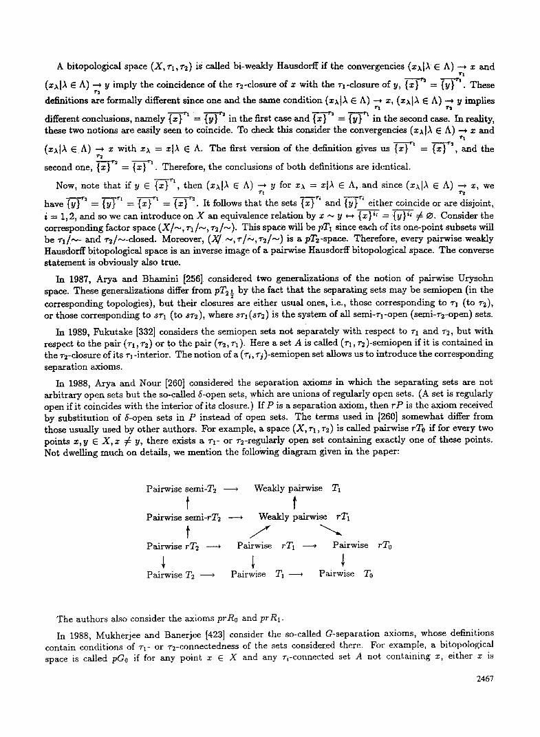
In 1988, Arya and Nour [260] considered the separation axioms in which the separating sets are not arbitrary open sets but the so-called 6-open sets, which are unions of regularly open sets. (A set is regularly open if it coincides with the interior of its closure.) If P is a separation axiom, then rP is the axiom received by substitution of 6-open sets in P instead of open sets. The terms used in [260] somewhat differ from those usually used by other authors. For example, a space (X, ~'1 ,v2) is called pairwise rTo if for every two points x, y E X, x ~ y, there exists a vl- or r2-regularly open set containing exactly one of these points. Not dwelling much on details, we mention the following diagram given in the paper:

Pairwise semi-T2 , Weakly pairwise T1

t t Pairwise semi-rT2 ~ Weakly pairwise rTl

Pairwise rT2 ~ Pairwise rT1 , Pairwise

PairwiseT2 ~ Pairwise T1 ~ Pairwise To

rY0

The authors also consider the axioms prRo and prRl.

In 1988, Mukherjee and Banerjee [423] consider the so-called G-separation axioms, whose definitions contain conditions of rl- or r2-connectedness of the sets considered there. For example, a bitopological space is called pGo if for any point x E X and any Ti-connected set A not containing x, either x is

2467

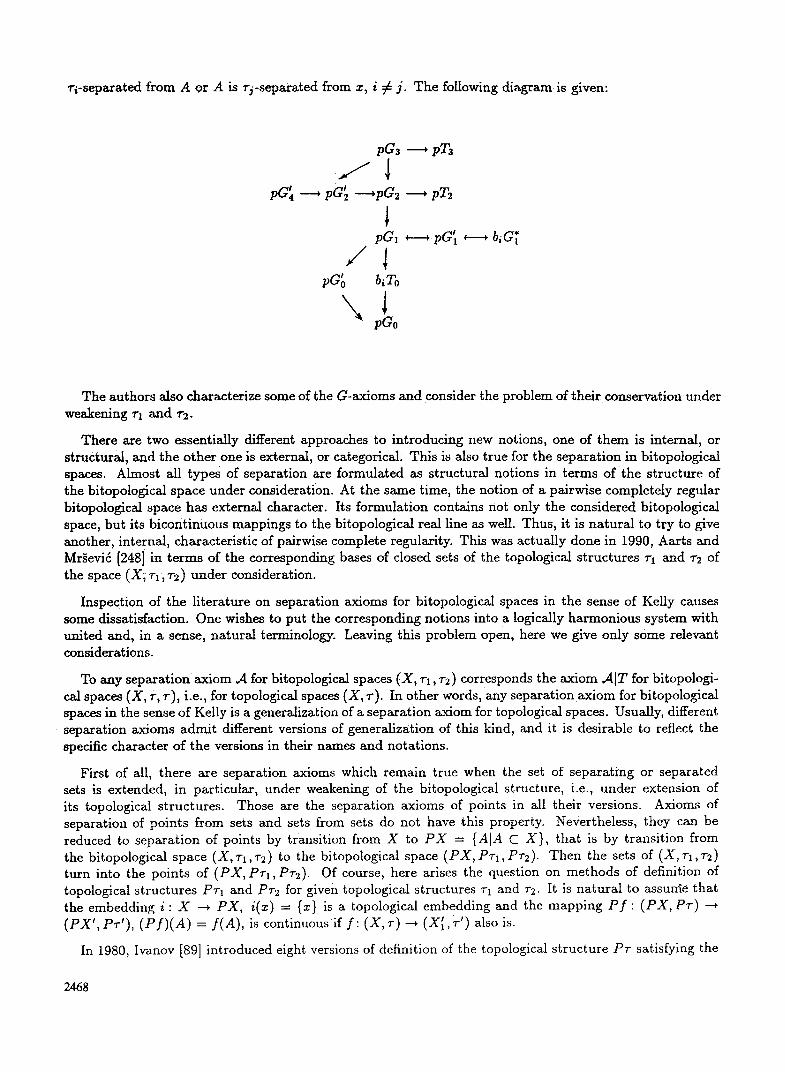
rl-separated f rom A or A is rj-separated from z, i # j . The following diagram is given:

pG3 ' pTa

J " l , pG' ,pG , pT2

pG1 ( ~ pG~ ,

/ 1 pG'o bi To

pGo

b~G~

The authors also characterize some of the G-axioms and consider the problem of their conservation under weakening rl and r2.

There are two essentially different approaches to introducing new notions, one of them is internal, or structural, and the other one is external, or categorical. This is also true for the separation in bitopological spaces. Almost all types of separation are formulated as structural notions in terms of the structure of the bitopological space under consideration. At the same time' the notion of a pairwise completely regular bitopological space has external character. Its formulation contains not only the considered bitopological space, but its bicontinuous mappings to the bitopological real line as well. Thus, it is natural to try to give another, internal, characteristic of pairwise complete regularity. This was actually done in 1990, Aarts and Mr~evid [248] in terms of the corresponding bases of closed sets of the topological structures rl and r2 of the space (X; r l , r2) under consideration.

Inspection of the literature on separation axioms for bitopological spaces in the sense of Kelly causes some dissatisfaction. One wishes to put the corresponding notions into a logically harmonious system with united and, in a sense, natural terminology. Leaving tiffs problem open, here we give only some relevant considerations.

To any separation axiom A for bitopological spaces (X, r~, r2) corresponds the axiom A[T for bitopologi- cal spaces (X, r, r ) , i.e., for topological spaces (X, r) . In other words, any separation axiom for bitopological spaces in the sense of Kelly is a generalization of a separation axiom for topological spaces. Usually, different separation axioms admit different versions of generalization of this kind, and it is desirable to reflect the specific character of the versions in their names and notations.

First of all, there are separation axioms which remain true when the set of separating or separated sets is extended, in particular, under weakening of the bitopological structure, i.e., under extension of its topological structures. Those are the separation axioms of points in all their versions. Axioms of separation of points from sets and sets from sets do not have this property. Nevertheless, they can be reduced to separation of points by transition from X to P X = {A]A C X}, that is by transition from the bitopological space (X, r i , r2) to the bitopological space (PX, Prl, Pr2). Then the sets of (X, r~,r2) turn into the points of (PX, Prl, Pr2). Of course, here arises the question on methods of definition of topological structures Prl and Pr2 for given topological structures rl and r2. It is natural to assurrie that the embedding i : X --* PX, i(x) = {z} is a topological embedding and the mapping P f : (PX, Pr) - , (PX' , Pr'), (P f ) (A) = f(A), is continuous if f : (X, r ) --, (X~, r ' ) also is.

In 1980, Ivanov [89] introduced eight versions of definition of the topological structure Pr satisfying the

2468

above conditions. These structures are defined by their bases, namely:

1. {PGIG 6 r},

2. {O, GIG e r}, 3. {PG, QGIG 6 r}

4. {PG, PG U P(X \ G)IG 6 r},

5. {QG, QG M Q(X \ G)IG 6 r},

6. {PG, QG, QG N Q(X \ G)IG 6 v},

7. {PG, QG, PG r P(X \ G)IG 6 r},

8. {PG, QG, PG N P(X \ G); QG M Q(X \ G)[G 6 r},

where PA = {BIB C A}, QA = {BIB C X, B N A # r Apparently, only one of these versions, (4), has been studied systematically, while the others are still

awaiting havestigation.

2,2. C o n n e c t e d n e s s . For the last few years, the theory of connectedness of bitopological spaces was developed mainly by generalizing its already well-known notions and results and by turning to new structural forms of connectedness (their categorical aspect will be considered in the next subsection). The main role in these generalizations is played by semiopen (semiclosed) sets. Here one considers semiopen sets with respect to the topological structures rl and ~-2 separately, as well as, so to say, mixed ( i , j )-semiopen sets, i ~ j . A set A is said to be (i , j)-semiopen in the bitopological space (X, ~'1, ~-2) if there exists U 6 r / s u c h t h a t U c A c U r J .

In 1987, Arya and Nour [258] consider a notion of local semiconnectedness of a bitopological space. It naturally generalizes the notion of local semiconnecteduess of Birsan [14], 1968, who calls a bitopological space (X, r l , ~'2) ~-i-locally semiconnected with respect to ~'i if for every point x 6 X and every n-open set U containing x there exists a pairwise semicormected set U' 6 r / s u c h that x 6 U' C U.

A bitopological space (X,~-1,7-2) is called locally semiconnected if it is ~-l-locally semiconnected with respect to vz and, at the same time, ~'2-1ocally semiconnected with respect to 7-1.

Unfortunately, these definitions seem to be insufficiently thought out, which is not untypical for other authors, as well. Here the phrases "with respect to vi," "with respect to ~'1," and "with respect to r2" are superfluous. In fact, we are dealing with a property of the topological structure Vl and, independently, with a property of the topological structure ~'2 in the bitopological space (X, ~'1, ~'2)- This property can be stated as follows:

We consider pairwise semiconnected sets of the bitopological space (X, vl, ~'2) and require that Vl and, independently, ~'z have bases consisting of such sets.

In [258], one finds rather simple statements and examples concerning the pairwise connectedness, pairwise semiconnectedness, pairwise local connectedness, and pairwise local semiconnectedness. Thus, it is proved that every pairwise semiconnected component is the maximal pairwise semiconnected set, that different components have empty intersection, that the component of a point is the intersection of the ~-l-semiclosure of its component with its v2-semiclosure and so on. The authors introduce notions Of the pairwise complete semidisconnectedness and the pairwise total semidisconnectedness of a bitopological space and a notion of its weak pairwise total semidisconnectedness. They also study the simplest properties of these notions. One can find some of these notions and results in 1986, Mukherjee [418].

In 1987, Arya and Nour [259] consider the notion of s-connectedness. A bitopological space (X, ~'1,7-2) is called (i, j )-connected between its nonempty subsets A and B if there exists no ~-/-semiclosed and ~-j- semiopen set F containing A and having empty intersection with B, A C F C X \ B. (X, 7-1,7-2) is called pairwise s-connected between A and B if it is (1.2)-s-connected and (2.1)-s-connected between A and B.

2469

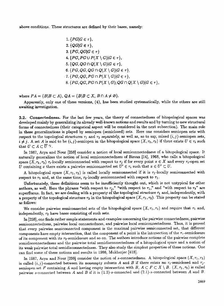
The authors prove some relevant s tatements . In particular, they give the following diagram:

pairwise connectedness

pairwise semiconnectedness pairwise cormectedness

pairwise s - connectedness"

between A and B

In 1990, Arya and Nour [261] s tudy quasisemicomponents and the relationships between them and semicomponents. In particular, pairwise semiconnected bitopologicM spaces are considered.

In 1988, Di Maio and Noiri [300] consider two weak forms of connectedness, which are defined by the corresponding operations of closure (0-closure and 6-closure). It is a pity that the reviews give no idea of the true contents of the paper, because we have had no possibility to see the paper itself.

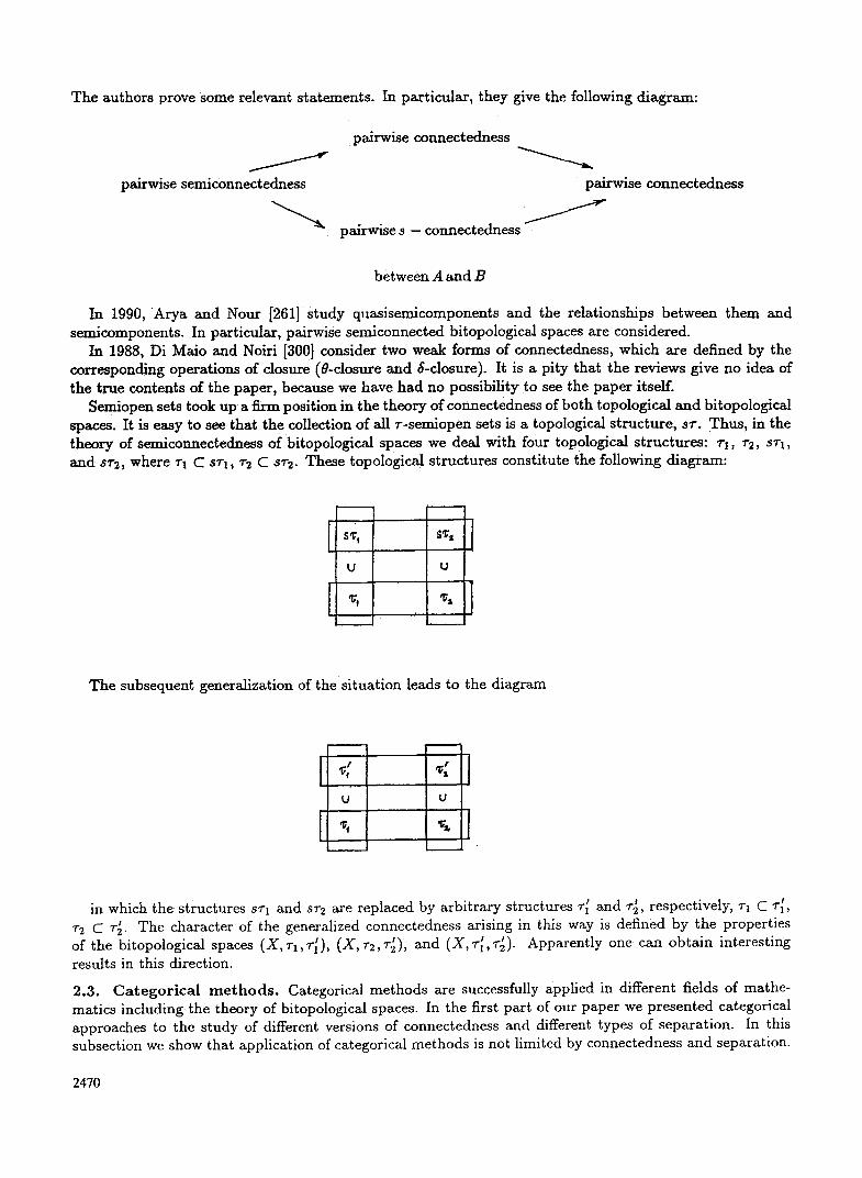
Semiopen sets took up a titan position in the theory of connectedness of both topological and bitopological spaces. It is easy to see that the collection of all r -semiopen sets is a topological s tructure, s~'. Thus, in the theory of semiconnectedness of bitopological spaces we deal with four topological structures: rl , r2, st1, and st2, where vl C st1, r2 C st2. These topological s tructures constitute the following diagram:

U U

The subsequent generalization of the si tuation leads to the diagram

[W u tJ

-I

in which the structures s~'l and s~-2 are replaced by arbitrary structures ~r~ and ~-~, respectively, ~-1 C ~'~, T2 C ~-~. The character of the generalized connectedness arising in this way is defined by the properties of the bitopological spaces (X, 7"1,r~), (X, 7-2, r~), and (X, ~-~, ~'~). Apparently one can obtain interesting results in this direction.

2.3. C a t e g o r i c a l m e t h o d s . Categorical methods are successfully applied in different fields of mathe- matics including the theory of bitopological spaces. In the first part of our paper we presented categorical approaches to the study of different versions of connectedness and different types of separation. In this subsection we show that application of categorical methods is not limited by connectedness and separation.

2470

Nevertheless, we begin with 1990, Rabrenovid [439], where new types of discontinuity in bitopological spaces are introduced and then used to give certain characteristics of the main separation axioms. Unfortunately, the author uses nonstandard notation. As is usual, he starts by fixing a class P of bitopological spaces, which is considered as the parameter of the theory. A bitopological space is called P-totally disconnected if all its components of P-connectedness are one-point sets. The class of all such bitopological spaces is denoted by P - T D . The conditions are given when P - D T = wpTo, pTo-TD = pTo, and pTo-TD = aT1, where a E { M N p , wp, p, rap}.

A bitopological space is called P-totally separated if all its P-quasicomponents are one-point sets. The class of all such bitopological spaces is denoted by P-TS . It is proved that this class is closed with respect to products and weak subobjects, P C P - T S C P-TD. The author gives the conditions for P - T S = wpTo, pTo-TS = pTo, and P - T S = O~Tl, where c~ e {wp ,pMNp, mp}, and for o~TI-TS = o~Ti, where c~ e {wp, p}, i = {2,2�89 P - T S = wp C T2. Here wp C T2 is the class of all bitopologicai spaces with the following property: for every two distinct points x and y of the bitopological space there exists its bicontinuous mapping f into RL,R such that f ( x ) = 0 and f (y ) = 1, or f ( x ) = 1 and f (y ) = O.

A bitopological space (X, vl, 7-z) is called P-zero dimensional if it is not P-connected between the vl-closed sets F and the points z E X \ F and it also is not P-connected between the r2-closed sets F and the points x E X \ F . The class of all such bitopological spaces is denoted by P-ZD. The case when P has the so-called property of finite intersections is studied separately. This property is formulated as follows. Consider the inverse images of the ~'i-open sets for all bicontinuous mappings of arbitrary bitopological spaces into the bitopological spaces of the class P. Such sets are called i-P-open. It is required that any finite intersection of i-P-open sets also be i-P-open, i = 1, 2. One proves a series of statements about bitopological spaces of the class P - Z D , including certain characteristics of separation, e.g., (wpT3-ZD) O wpT1 = wpT3.

A bitopological space (X, ~-I, r2) is called P-strongly zero dimensional if it is not P-connected between every ri-closed set A and ri-closed set B, i r j , i , j , = 1,2. The class of all such bitopological spaces is denoted by P - S Z D . Two rather special statements concerning this class are proved. The first one concerns a peculiar heredity in the class P - S Z D , and in the second, the cases P = {DL,~t}, P = {/L,R}, P = {RL,R} are considered. Here the bitopological spaces DL,R, IL,R, and RL,R are the sets {0, 1}, [0, 1], and the set R of all real numbers, L and R are left and right topologies defined by the natural order on these sets.

Paper [369] (Jelid Milena, 1987) is devoted to a categorical concept of connectedness. In this paper the Preuss theory is applied to the category of bitopological spaces. Paper [368] (Jeli6 Milena, 1987) is devoted to the categorical inductive dimensions p-indcBX and P-Inden X of bitopological spaces. Here eB is just the chosen class P (again a new notation!). It is known that to introduce the inductive dimension we need an inductive transition from the dimension of the whole space to the dimension of partitions between points and closed sets (for indX) and between closed sets (for IndX). For bitopological spaces there is no notion of a closed set. Therefore, when constructing the bitopologicaI inductive dimension we must find a suitable substitute. This was done in 1974, Dvalishvili [57] and translated into categorical language in [368].

2.4. C o m p a c t n e s s . The notion of compactness of a bitopological space turned out to be so delicate that up to now it has no definition which would be suitable in every respect. This is so in spite of and, possibly, due to the fact that there is a considerable number of definitions of this notion in the literature. In recent years the problem of the "true" definition of compactness continued to attract attention.

It is known that if a topological space (X, v) is compact and ~- is a Hausdorff topological structure, then ~- is minimal in the class of all Hausdorff topological structures. It is natural to suppose that a similar state- ment should be true in the class of all pairwise Hausdorff bitopological spaces. According to this principle, the minimality of a bitopological structure (Vl, v2) will be a necessary condition for compactness of the bitopological space (X, r l , r2). Almost all known definitions of compactness of bitop01ogical spaces satisfy this condition. For example, let (X, vl, v2) be an arbitrary KN-compact pairwise Hausdorff bitopological space. Every proper 7-i-closed set of this space is r/-compact, i r j, i, j = 1, 2. Further, let (X, ~'[, v~) be another pairwise Hausdorff space such that r~ C rl, ~-~ C v~. Let F be a proper ri-closed subset of X and let z~F . Then for any point y E F there exist sets Uy and Vy such that y E Uy E ~'j, x E Vy E ~'~, and Uy M Vy = ~. The sets U~ly E F constitute a ri-open cover of F, and because of the KN-compactness of

2471

(X, rl ,r2) there exist Uy~, . . . , Uy~ covering F. This implies tqF = ~ and hence the point z does

not belong to the 7"~-closure of F. I t follows that the set F is r~-closed. Thus, we have proved that r/~ = ri, i = 1, 2, and therefore (X, 1"1, r2) is a minimal pairwise Hausdorff bitopologieal space.

Now let us consider the following instructive example. We borrowed it from [375], where it is given on another oceaaion.

Let X be an arbitrary set, let r~ be the maximal Tl-topology on X, i.e., the discrete topological structure, and let rm be the minimal Tl-topology which consists of the empty set and the complements to all finite subsets of X. Then (X, ra, r , , ) is a pairwise Hausdorff bitopological space since if x ~ y are points of X, t h e n z E U = {x} E rd, y E V = X \ ( x } E r,~, a n d U f q V = O. Now, (X, rd, r , , ) is a K N - c o m p a c t bitopological space. In fact, any r,~-open cover of F C X obviously contains a finite cover, and therefore any such set is r,~-compact. On the other hand, any r,,,-closed proper subset of X is finite and hence compact. Therefore , both (X, rg, rm) and (X, rr,, rd) are KN:compact pairwise Hausdorff bitopological spaces. Consider their product (X • X, rd X r~a,rm • 7"d).

In X • X, any vertical set {x} • X is 7"d • tin-closed, and any horizontal set X • {y} is ~',, x rd- open. Thus, for any vertical set we can consider the rm • 1"d-open cover by all horizontal sets. This cover contains no finite subcovering and so every vertical set will be rd • ~-ra-closed but not v,~ x r~-compact. It follows that (X • X, ~'d • ~',~, 7",~ • vd) is not a KN-compact pairwise Hausdorff bitopological space (the property of KN-compactness is not multiplicative). One can also prove that (X • X, vd x r,~,r,~ x vd) is not a minimal pairwise Hansdorff bitopological space (the property of minimality of pairwise Hansdorff bitopological spaces is not multiplicative). This fact is proved in [375].

As already mentioned, there is no sufficiently satisfactory definition of compactness of bitopological spaces. It is known that the notions of KN-compactness, K-compactness, and FHP-compactness differ by wordings only. In reality, this is one and the same notion, which is often called the pairwise compactness. Is it possible to take it as a base, i.e., to give an apt definition of compactness of a bitopological space (X,~'l,r2) by adding a certain additional condition to the pairwise compactness? At the minimum, one should require that such a definition must be multiplicative and symmetric with respect to ~'1 and r2.

Let a bitopological space (X,v~,v2) be compact in this sense. Then (X,~'2,~'1) is also compact and, therefore, (X • X, ~'1 x v2, ~'2 x 7"~) is compact, too. If ~'1 is the trivial topological structure, i.e., rl = {X, O}, then (X, T1) is a compact topological space. Assume that vl is nontrivial, i.e., there exists an F E C~-, F r O, F r X. Then F x X is a nonempty proper rl • v2-closed set, which is compact because of the pairwise compactness of (X • X, rl • ~-~, ~'2 • ~'1). Consider any ~q-open cover s of X. Then X • s = {X x GIG E s} is a 7-2 • r l -open cover of F x X. Since the latter is v2 • ~'l-compact, the cover X • s contains a finite subc0vering X x G1, X • G2, . . . , X • G, . Now, the sets G1, G2, . . . , Gn constitute a finite cover of X, and so the topological space (X, Vl ) is compact. The compactness of (X, v2) is proved similarly.

Thus, for any definition of compactness of a bitopological space which includes the condition of pairwise compactness and guarantees the multiplicativity of compactness as well as its symmetry with respect to both topological structures r l , r2, the compactness of (X, r l , r2) implies that of (X, r~ ) and (X, v2).

On the other hand, if (X, rx, r2) is pairwise Hausdorff and (X, ~'~ ) and (X, r2 ) are compact, then r~ = ~'2. Thus, for any definition of compactness which includes the condition of pairwise compactness and guaran-

tees the multiplicativity of compactness as well as its symmetry with respect to both topological structures rl , ~'2, we shall have r~ = r2 for every compact pairwise Hausdorff bitopological space.

All these complications arising in connection with the choice of definitions of the fundamental bitopo- logical notions train us little by little to the following principle.

We shall say that a bitopological space (X, ~-~, r2) possesses the bitopological version of a topological property P (has the property bitop P) if the topological space (X • X,T~ • ~-2) has the property P.

According to this principle, a bitopological space (X,r~,r~) is bicompact (resp., bi-Hausdorff, etc.) if (X x X, 7q • is compact (resp., Hausdorff, etc.). This approach to bitopological analogues of topological notions creates no troubles. Moreover, such a system of notions is automatically transferred to arbitrary bitopological spaces (and not only those in the sense of Kelly).

Along with the different versions of compactness, the corresponding versions of almost compactness are considered in the literature. Almost compactness differs from compactness by the condition that the space

2472

is covered not with the chosen sets, but with their closures. For example, in 1977 Vasudevan and Goel [474] introduce the notion of C-compactness. A bitopologieal space (X, r~, r2) is called G-compact if for any proper ri-closed set A and any rj-open cover of A there exists a finite system of elements of this cover whose rFciosures cover A . It is natural to caLl this notion the KN-almost compactness (almost KN-compactness) , the more so as the term "C-compactness" is sometimes used in a quite different sense.

In 1988, KariofiLlis [375] considered another notion of almost compactness . A bitopological space (X,r~, rz) is called almost compact if for any point z E X, any rj-open cover (UxlA E A) of X \ {z}, and any ~'j-open set V containing z there exists a finite system of sets Ux,, ,~i E A, such that their ri- closures together with the ri-closure of V constitute a cover of X. In [375] it also is proved tha t if (X, r l , rz) is an almost compact pairwise Hansdortf bitopological space, then (1"1, rz) is minimal among the pairwise Hausdorff bitopological structures on X. Moreover, it is proved that this notion of almost compactness coincides with the notion of minimality in the class of the so-called semiregular bitopological spaces, which are defined by the author as the pairwise Hausdorff bitopological spaces (X, r l , r2) such that the (i,j)- regularly open sets constitute a base of the topological structure ri, i , j = 1,2, i # j ' . Here a set is called (i , j)-regtdarly open if it coincides with the r/Anterior of its rj-closure.

Note that the term "almost compactness" is sometimes used in another sense, see, e.g., 1982, Mukherjce [147] and even 1988, Kariofillis [376].

All versions of the notion of almost compactness are generalized by the notion of a-compactness. The generalization is that instead of the closure one uses another operation a defined on the elements of the topological structure. UsuaLly, one requires that G C aG. Such a generalization was studied, for example, in 1985, Abd. EbMonsef, Ramadan, and Machhewr [250]. The same term "a-compactness" was used in 1989, Abd. E1-Monsef and Ramadan [249], but in quite different sense.

One should also mention the investigations on pairwise semiciosedness of bitopotogical spaces, see, e.g., 1986, Milena Jelid [366]. Instead of open covers, the author considers semiopen covers (covers by semiopen sets), usual closures of their ciements constitute a cover of X. In our terminology, this is investigations on almost semicompactness.

The lack of generally estabhshed terminology is particularly striking in the theory of compactness of bitopological spaces. Different authors use different names for the same notions, while quite different notions are given the same names.

2.5. O t h e r spec ia l p r o p e r t i e s . A new method for singling out special classes of bitopologieal spaces is found in 1989, Arkhangel'skii and Bokalo [254]. Though by no means devoted to bitopological spaces, this paper is of certain interest for us. It starts with the following definitions.

We say that two topological structures coincide at a point if their filters of neighborhoods of this point coincide.

Let 8 and/z be two properties of subsets of topological spaces. The authors let gu(X, ~'), or simply g t, if it causes no confusion, denote the set of all nonempty subsets with the property # in the topological space (X, r ) . For each Y E E~, let Eq(Y) be the set of all nonempty subsets with the property 8 in (Y, f lY). Let Eo,~ denote the system consisting of all such sets.

A topological structure rx is said to be a (8,/t)-face of a topological structure r2 if for every Y E Et,(X, r2) there is a set Z E ga(Y) such that r l lY and r2lY coincide at every point of Z.

The above definitions allow the authors to consider the class T0,, consisting of all (X, ~q, ~'2) such that r, is a (0,#)-face of r2. For every set X put To,~,(X) = {(X, ri,~'2)l~-i is a (O,/~)-face of ~'2}.

In particular, the class Tan = Tt,t, where t is the trivial property "to be a subset," is considered in [254]. This class is easily seen to consist of all bitopological spaces X such that every nonempty subset Y C X has a point whose ~-I IY- and ~-2 IY-filter of neighborhoods coincide.

It is also easy to see that for every X and r, the bitopological space (X, ~-, ~-) belongs to the class To,~, for any topologicaI properties O and/~.

From this point of view, the fact that a bitopological space (X, ~-I, ~-2) belongs to this or that class T0,, reflects the character and the extent of coincidence (lack of coincidence) of topological structures ~-1 and r2 defined on the same set.

In general, the extent of such coincidence can be estimated by different methods. For example, we can directly compare rl and r2 by considering their intersection r = rl Nr2, which is also a topological structure.

2473

It seems to be intuitively clear that the less is rl n r2, the greater is the difference between T1 and r2. If 7;I f'lrz = {~ ,X} , then rl and 7"2 seem to have nothing in common.

Another method of estimating the degree of coincidence of rl and rz is based on the above-described idea of [254], Consider the set J (X , r l , r z ) of all subsets of X on which r~ and r2 coincide. Once more, it s e e m s to be intuitively dear that the greater is d(X, rl,r2), the nearer are rl and r2 to each other.

However, consider the following example. Let X = [1, 2], X ' = (1,2), let r ' be the usual topological structure on (1, 2), and let

r~ = (6~'u {I}IG' E r'} U {~,X},

r~. = {c'u {2}IG' E r'} u (~,x}.

Every rl-open set different from ~ and X contains the point 1 and does not contain the point 2, whereas every *'z-open set different from ~ cad X does not contain 1 and contains 2. It follows that t i n t 2 = {~ ,X}. Estimating the coincidence by ~'l I"1 rz we come to the conclusion that ~-1 and 7-2 are remote from each other. On the other hand, rx and 7"2 coincide on the set X' , which differs from X by two points only, and so estimating the coincidence by 3(X, r1,rz) we convince ourselves that T1 and r2 almost coincide. Thus, different approaches to the estimate of coincidence can give us exactly opposite results.

This example shows that estimating the extent of coincidence of two topological structures is a highly delicate thing.

From the bitopological point of view the extent of coincidence of two topological structures rl and rx defined on the same set corresponds to the degree of proximity of the bitopological space (X, ~'1, r2) to the bitopological spaces of type (X, r, r ) , i.e., the degree of proximity of the bitopological space (X, r~, rz) to topological spaces. It seems natural to look for the topological space (X, r ) nearest to (X, rx, r2) among the topological spaces (X, r ) such that r lies between inf{rl , r2} mad sup{r1, r2}. Apparently, it is reasonable to consider the topological space (X, r ) with r = {G'U {1, 2}[G' E r '} U {~} as the nearest to the bitopological space (X, r l , r2) considered in the above example.

2.6. M a p p i n g s . The study of different classes of mappings of bitopological spaces, not necessarily bicon- tinuous, was continued in recent years.

The corresponding subsection of the first part of our paper shows that investigations of this kind were performed very intensively more than five years ago and that the types of mappings of bitopological spaces that can be found in the literature are highly diversified. Here we limit ourselves to two papers.

The first is 1987, Banerjee [267], where five types of mappings f : (X, r l , ~'2) ~ (X' , r~, r~) are considered. (I) ( i , j )-strongly 8-continuous mappings: for every point z E X and every r1-neighborhood V of f ( z )

there exists a ri-neighborhood U of z such that f(U "ri ) C V. (II) (i, #)-almost strongly 8-continuous mappings: for every z E X and every , / -neighborhood V of f(~)

there exists a n-neighborhood U of z such that f(O"~ ) C (fr,-;),.,. (III) (i,j)-~-continuous mappings: for every z E X and every rl-neighborhood V of f(z) there exists a

rl-neighborhood U of z such that f(O"J )~, C (fry;)~,.

(IV) (i,j)-almost continuous mappings: for every z E X and every r~-neighborhood V of f(z) there exists

a n-neighborhood U of z such that f(U) C (V";)'i" (V) (i , j)-a-continuous mappings: for every z E X and every r[-neighborhood V of f (z) there exists a

ri-neighborhood U of z such that f ( 0 "~j ) C V~;. The author gives a diagram of implications relating these notions, which looks rather complex. In reality, it is simply a sequence of implications t --* II ~ IIt --* IV --* V and their compositions. The second paper is 1987, Maheshwari and Tiwari [405]. In a sense, it completes a cycle of papers of

the authors. Along with the well-known pairwise continuous, i.e., bicontinuous mappings of bitopological spaces (type I0) the following types of mappings are considered.

(I) almost pairwise continuous mappings: for every point z E X and every r[-neighborhood V cff f(z) there exists a r~-neighborhood U of z such that f(U) C (f"";),.,.

i

(II) 0-pairwise continuous mappings: for every z E X and every r~'-neighborhood V of f(z) there exists a

ri-neighborhood U of z such that f((j~i ) C V";.

2474

(III) weakly pairwise continuous mappings: for every x E X and every r~-neighborhood V of f ( z ) there exists a r i -neighborhood U of x such that f(U) C ~r~.

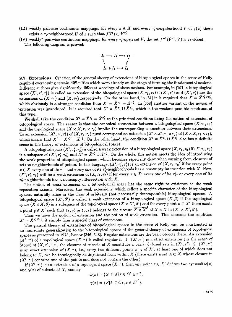
(IV) weakly* pairwise continuous mappings: for every r~-open set V, the set f - 1 (~r~ ; V) is 7"i-closed. The following diagram is proved:

/o , /1 , / 2 \ / h+14 , h

2.'/. E x t e n s i o n s . Creation of the general theory of extensions of bitopological spaces in the sense of Kelly required overcoming certain difficulties which were already on the stage of forming the fundamental notions. Different authors give significantly different wordings of these notions. For example, in [197] a bitopological space (Z ' , r ' , • ) is called an extension of the bitopological space (X, ~'1, T2) if (X' , v~) and (X' , r~) are the extensions of (X, ~'1 ) and (X, v2) respectively. On the other hand, in [61] it is required that X = )~TIvr;, which obviously is a stronger condition than X ~ = .~rl = .~r;. In [358] another variant of the nobion of

:extension was introduced. It is required that X ' = , ~ U X~;, which is the weakest possible condition of this type.

We shall take the condition X t = ~r~ = .~T; as the principal condition fixing the notion of extension of bitopological space. The reason is that the canonical connection between a bitopological space (X, 7-1, v2) and the topological space (X x X, vl • v~) implies the corresponding connection between their extensions. To an extension ( Z ' , r~, r~) of (X, ~'1, r2) must correspond an extension (X' x X ' , r~ x r~) of ( Z x X, rx x ~-2), which means tha t X ' = - ~ = -~r~. On the other hand, the condition X ' = X~[ U X ~ also has a definite sense in the theory of extensions of bitopological spaces.

A bitopological space (X' , ~'[, ~'~) is called a weak extension of a bitopological space (X, ~-~, r2) if (X, r~, v2) is a subspace of (X' , r~, v~) and X ' = ~7 r[ U .~r;. On the whole, this notion meets the idea of introducing the weak properties of bitopological spaces, which becomes especially clear when turning from closures of sets to neighborhoods of points. In this language, (X' , v~, r~) is an extension of (X, r l , ~'2) if for every point x E X every one of its ~'~- and every one of its v~-neighborhoods has a nonempty intersection with X. Now, (X' , r~, r~) will be a weak extension of (X, 7-i, ~'~) if for every x 6 X ' every one of its r~- or every one of its r~-neighborhoods has a nonempty intersection with X.

The notion of weak extension of a bitopological space has the same right to existence as the weak separation axioms. Moreover, the weak extensions, which reflect a specific character of the bitopological spaces, naturally arise in the class of arbitrary (not necessarily decomposable) bitopological spaces. A bitopological space (X' , fl') is called a weak extension of a bitopological space (X, fl) if the topological space (X x X, fl) is a subspace of the topological space (X x X' , fl') and for every point x 6 X ' there exists

a point y E X ' such that (x, y) or (y, x) belongs to the closure X x "X# of X x X in (X' x X',/3!). Thus we have the notion of extension and the notion of weak extension. This concerns the condition

X ' = _~r[w~; it simply fixes a special class of extensions. The general theory of extensions of bitopological spaces in the sense of Kelly can be constructed as

an immediate generalization to the bitopological spaces of the general theory of extensions of topologicM spaces as presented in 1973, Ivanov [346,348]. Regular extensions are the basic objects there. An extension (X ' ,v ' ) of a topological space (X,~') is called regular if: 1. ( X ' , r ' ) is a strict extension (in the sense of Stone) of (X, v), i.e., the closures of subsets of X consti tute a basis of closed se ts in (X' , ~-'). 2 . (X' , v') is an exact extension of (X,T), i.e., every two different points x, y of X' , at least one of which does not belong to X, can be topologically distinguished from within X (there exists a set A C X whose closure in (X' , r ' ) contains one of the points and does not contain the other).

If (X ' ,~ ' ) is an extension of a topological space (X, v), then any point x E X' defines two system~'w(x) and 7(x) of subsets of X, namely

: {a' n e c ' �9

7(z) : {FIFE Cv, x E P~" }.

2475

The system w(x) consists of nonempty sets closed in (X, r) , to(x) C r , and the system 7(x) consists of nonempty sets closed in (X, r) , 7(x) C (Tr = { F I X \ F E r}. The system w(x) has the following properties:

1. G1 E 0J(x), G2 E w(x) --~ G1 N G2 G to(x); 2. G1 E w(x), G2 E r, G1 C G~ --, G, E w(x). Any nonempty system w of nonempty open sets having these properties is called an open filter. The system 7(x) has the following properties: 1. F, 13 F2 e 7(x), F, E C7", F2 e C7- --~ F t e 7(x) or F2 e 7(x); 2. F1 e 7(x), F2 E G,, F1 C F2 --* F2 E 7(z). Any nonempty system 7 of nonempty closed sets having these properties is called a closed cofilter. There is one-to-one correspondence (a dual relation) between open filters w and closed cofilters 3' in a

topological space (X, r) , namely:

7 @ ) = {FIFECr, X\F w}, = {GIGE r, X\G 7}, = t o .

In particular, for every point z of an extension (X', r ' ) of a topological space (X, r ) we have 7(w(x)) = 7(x) a n d =

The following construction always gives us a regular extension of an arbitrary given topological space

Let f~ be a set of open filters in (X, r ) containing no filters of type w(x), x E X. We add this set to X and introduce on the obtained set X ' = X O f~ a topological structure r ' . A basis of this topological structure is given by the sets of the form G LI {wiG E w G f~}.

In [346] it is proved that the topological space (X', r ' ) is a regular extension of (X, r ) . It is called the extension obtained by adding to X the set ~2 of open filters in (X, r) ,

The dual construction gives us a regular extension (X' , r ' ) of (X, r ) obtained by adding to X the set F of closed cofilters in (X, r) . Here F should contain no closed cofilters 7(x) in (X, r ) , x E X.

If (X' , r ' ) is a regular extension of a topological space (X, ~-), then it is canonically isomorphic to an extension obtained by adding to X the set ~2(X') = {w(x)lx E X ' \ X } or the set I ' (X ' ) = {7(x)[x E X ' \ X } .

Now, passing to extensions Of bitopological spaces, we presently consider only the class of the bitopological spaces in the sense of Kelly, i.e., of decomposable bitopological spaces onto which we shall t ry to extend the notion of regular extensions. For simplicity of the presentation we limit ourselves by the extensions of bitopological spaces only. The weak extensions cause, in principle, no additional difficulties.

As in the case of the topological spaces, the notion of a regular extension of a bitopological space includes the notions of strict extension and of exact extension.

(X,r~,r~) is a strict extension if (X',r~) and (X',r~) are strict extensions of topological spaces (X, rl) and (X, ra) respectively.

There are different versions of the notion of exact extension. (X', r~, 4 ) is an exact extension if (X' , r~) and (X' , r~) are exact extensions of topological spaces (X, rl )

and (X, r=) respectively. (X', r~, r~) is a weakly exact extension if every two points x, y, at least one of which does not belong to

X, can be topologically distinguished from within X, i.e., there exists a set A C X such that its closure in (X', r~) or its closure in (X", r~) contains one of the points and does not contain the other.

A strict and (weakly) exact extension of a bitopological space will be called a (weakly) regular extension. If (X', r~, r~) is a regular extension of (X, rl , r2), then any point x G X' defines open filters to1 (x) and

to2(x) in the topological spaces (X, r~ ) and (X, r2), respectively (as well as closed cofilters 7, (x) and 72(x)). For i = 1,2, the set f'ti(X') = {toi(x)[x E X ' \ X} defines an extension ( X ' , r ' ) of (X,~q) uniquely up to isomorphism of extensions. But f~l (X' ) and f~2(X') do not define, even up to isomorphism of extensions, an extension (X',r~,r6) of the bitopological space (X,r~,r~). For this it is necessary to know a one- to-one correspondence between the elements of f~l(X') and those of f~2(X') that is defined by all the correspondences to1 (:r) ,--, z ~ to2(x) for x E X' \ X. This is the principal difference between the theory of extensions of bitopological spaces and the theory of extensions of topological spaces.

2476

The following construction always gives us a regular extension of an arbitrarily given bitopological space (X, rl ,r2). For i = 1,2, let ~i be a set of open filters of the topological space (X, ri) which contains no filters of the form wi(x), x E X . (We can consider the corresponding sets Pl and F2 of closed cofilters, a s well.) Fix a one-to-one correspondence q0 : ~1 -'* 122 between the points of t h e s e s e t s . A d d t h e graph F~ of this correspondence to the set X. We obtain t h e s e t X ~ = X U F~, and define on it two topological structures r~ and r~. For i = 1, 2, the topological s tructure r[ on X ' is defined as the minimal topological structure containing all sets Gi U {(wl ,w2)lw2 = qo(wl), Gi E wi E f~i}, Gi E rl.

Here it is of interest to note that if (X, v~, r~) is a regular extension of (X, r~, r2), then the condition rl = r2 does not imply r~ = r~. This is true if q0 : f~1 ~ f~2 is the identical mapping.

Note also that the weak extensions of bitopological spaces are defined by arbitrarily chosen sets f~1 and f~2 of open filters with the above-mentioned restrictions and arbitrarily fixed partial (defined, possibly, not on the whole set f~l) many-valued mappings qo: f~l ~ f~2- Here we also have X ' = X U F~, but the graph F~ of q0 is defined as follows:

- if the mapping q0 is defined for w~ e f~ and w2 = qo(wl), then (wl,w2) E F~o; - if the mapping q0 is not defined for w i E f~, then wl E F~; - if w2 E ~2 is not an image of an element of f/l , then w2 E F~. The literature on extensions of bitopological spaces is mainly devoted to compactifications and comple-

tions. It is quite interesting, although not very extensive. It concerns not only different extensions, but also relationships between the properties of bitopological spaces and the corresponding properties of extensions. To be mentioned are, in particular, existence theorems for extensions satisfying requirements of one kind or another. See, for example, the cycle Doitchinov [301-305] devoted to the completions of quasitmiform and quasimetric spaces.

A system 9 / o f entourages of the diagonal A C X x X is called a quasiuniformity (a quasiuniform structure) if

1". U E g/, U c V c X x X -+ V E 91; 2". U~ eg / , U29/--+ U~ AU2 Eg/; 3*. For every entourage U E P2 there exists an entourage V E 9/such that V 2 C U, where

V 2 = { (x , z ) lx E X , z E X, there exists y e X such that (x,y) e V and (y ,z) e V} .

Let wl and w2 be two filters defined on the set X. Then, by Doitchinov's definition, (601, w2) --0 0 if for each entourage U E 9 / there are A E 031 and B E w2 such that A x B C U. The filter w2 is called a Cauchy filter in (X,9/) if there exists a filter wl such that (wl,w2) ~ 0. A quasiuniform space (X,9/) is called complete in the sense of Doitchinov if every Cauchy filter converges in (X,9/) to a point x E X, i.e., for any U E 9 / there is A e w such that A C U(z) = {yl(x, y) E V}.

The completion of a quasiuniform space (X, 9/) is constructed in [301] as follows. First of all, an equivalence relation for the Cauchy filters is introduced: namely, two Cauchy filters w

and w' are equivalent if for every filter wl the conditions (wl,w) -+ 0 and (wl,w') --+ 0 are equivalent. This relation divides the set of all Cauchy filters of (X, 9/) into disjoint equivalence classes. All such classes

consisting of filters not converging in (X, 9/) are added to the set X as the growth points of extension. On the set X* thus obtained, a quasiuniformity 9/* is introduced, so that (X*,9/*) proves to be a complete quasiuniform space.

This rather complex two-stage construction of completion, which uses arbitrary (not necessarily open) filters, can be replaced by a simpler procedure using open filters. This construction is defined in a situation more general than Doitchinov's, where axiom 3* is not used. Here, however, some complications appear, due to the fact that the operations of closure (operations of interior) defined by the systems of neighborhoods {V -1 (y)Iy e X} and {V(y)Iy e X } are not necessarily idempotent, and, thus, the topological structures rl and r2 on X are not defined a priori. After all, one can assume that vl and r2 aredefined even if axiom 3* is not fulfilled, i.e., one can pass to some weakening of axiom 3*. If this is undesirable, we can consider filters consisting of the interiors of the sets, which are always defined by systems of neighborhoods of points. We shall suppose that 9.1 defines a bitopological space (X, rl , v2) in the sense of Kelly. Then P2 defines on X a biuniformity (p~, p2) as well. Here p~ and p2 are systems of open covers of (X, rl ) and (X, r2) corresponding

2477

to ~. An open cover of (X,7-~) belongs to p~ if and only if for some g e ~ the cover {U-~(y.)ly e X} is a refinement of the given cover. Similarly, an open cover of (X, 7-2) belongs to p~ if and only if for some U the cover {U(y)ly e X} is a refinement of the given cover.

Thus, any quasitmiformity ~ on X defines a bitmiform space (X, pl, p2). Note that the construction of both general uniform structures pl and p2 is in no way connected with

axiom 3* of quasitmiformities. The fact is that any nonempty system p of open covers S of a topological space (X, 7-) is considered as a general uniform structure on (X, r ) if the following system of conditions is satisfied:

P1. If $1 is a refinement of $2, $1 E p, and Sz is an open cover of (X, 7-), then $2 E p. P2. If $1 E p a n d S z E p , t h e n S ~ Y S 2 E p . On the other hand, verification of the axioms P1 :and P2 for the systems Pl and p2 constructed from 92

does not use axiom 3", only axioms 1" and 2* are used. It is known [346] that any general uniform structure p on a topological space (X, 7") defines a completion

pX of (X, r) , which is constructed in the following way. An open filter w in (X, 7-) is called a p-Cauchy filter if each open cover s E p contains an element G of w.

A closed cofilter 7 in (X, 7-) is called a p-Cauchy cofilter if C7~ p. The minimal p-Cauchy filters in (X, 7-) bijectively correspond to the maximal p-Cauchy cofilters via the usual correspondence between open filters and closed cofilters.

An extension obtained by adding to X all minimal p-Cauchy filters (all maximal p-Cauchy cofilters) with the usual reservation (they should not coincide with w(x) (resp., 7(z)), z E X) gives us the completion pX. A quasiuniform structure P.I on X along with the general uniform structures pl and Pz defines their completions piX and p2X. One can construct different weak extensions of the bitopological space (X, 7-1,7"2) by considering them as a kind of completion of the given quasiuniform space (X, 92).

Doitchinov is interested only in extensions with some specially mentioned properties. Practically, he considers a pairing of minimal px-Cauchy filters with minimal p2-Cauchy filters, which gives pairs (Wl ,w2) such that for any entourage U �9 P.l there exists a set G1 x G2 C U with G1 �9 wl, G~ �9 w2. The set of all such pairs is denoted by ~2p~p2.

It is easy to prove that 12plp~ is the graph of a one-to-one correspondence between the set ~2p~ of coupled minimal pl-Cauchy filters and the set ~2p2 of coupled minimal p2-Cauchy cofilters. In other words, every element of each pair (wl,w2)from ~2p~p2 uniquely defines its partner and is uniquely defined by it. In fact, let (w~,w2) and (w~',w2) belong to ~2p~p2, let wl = w~ V w~ ~ = {G1 U G2[G1 �9 wa,G2 �9 w2}, and let s �9 pl.

Since s �9 p~, there exists an entourage U of the diagonal such that the cover {U-~(y)ly �9 X} is a refinement of s. On the other hand, since (w~,w2) and (w~',w2) belong to 12p,,p,, there exist G~ �9 w~, G~ �9 w2, G]' �9 w~', and G~ �9 w2 such that G~ x G~ C U and G~' x G~ C U, Then (G~ UG] ' )x (G~ x G~) C U and, therefore, G~ U G~ C U-l(yo) for some y0 �9 G~ x G~. But the cover {g-l(y)[y �9 X}, by condition, is a refinement of S, and so there is G~ E s which contains U-X(y0). Since G~ U G~' �9 w~ and G~ U G~' C U-l(yo) C G1, we have G1 �9 wl. This means that wl is a p-Cauchy filter. But, by construction of wl, we have inclusions w~ C w~, Wx C w~', and so, in view of the minimality of w~ and w~', we have w~ = w~ = w~'. We have proved that the second partner uniquely defines the first one. The converse is proved similarly.

Instead of p~X and pzX we can consider the truncated extensions tb~X and fi2X, in which only the coupled growth points are preserved. Adding to X the graph of the one-to-one correspondence defined by the pairing we obtain an 92-completion, which coincides with Doitchinov's completion when the latter

exists. It is also necessary to mention an early construction of a completion in 1978, Lindgren and Fletcher

[397]. The basic objects here are the bases of filters. If systems ~" and ~ (in the authors' notation) are bases of filters on a set X, then (~-,6) is called a pair base of filters. In a quasiuniform space (X,~)~ a point p �9 X is called a limit point of a pair filter (~-, 6) if p is a limit point of ~- in (X, 7"~ ) and a limit point of 6 in (X, 7"2). The authors denote by L(x) the filter generated by the system {U- ' (x ) IU ~ P2}, by R(x) that generated by {U(x)IU �9 92}, and by N(x) that generated by L(x) V R(x). For every x �9 X, (L(x), R(x)) is a pair base of filters. The pair base of filters (gv~, G~) is coarser than the pair base (~', 6) if the filters generated by the bases ~'~ and ~ are contained in those generated by ~" and G respectively. Two pair bases of filters (~"~, ~ ) and (.T'2, ~2) are equivalent if each of them is coarser than the other. A

2478

pair filter (jr, ~) converges to a point p if (L(p), R.(p)) is coarser than (.T', ~). A pair base of filters (Jr, ~) is a ~l-Cauchy base if for every U E ~ there exist F E ~" and G E

such that F x G C U. A quasiuniform space ( X , ~ ) is called pair complete if each ~-Cauchy pair base converges. Lindgren and Fletcher's completion can be constructed by using essentially the same procedure as was used for constructing Doitchinov's completion, but with different pairing. In [397], ~* denotes the minimal uniformity containing the quasiuniformity ~. It is proved that the quasiuniform space (X, ~1) is pair complete if, and only if, the uniform space (X, ~*) is pair complete. This shows t h a t Doitchinov's pairing is finer, and it better reflects the specific character of deviation of the quasiuniformity from uniformity. The pair completion does not detect deviations which are too strong. It is interesting to note that the corresponding example can be found exactly in [397], but it is given there on a quite different occasion. The authors compare their notion of pair completeness of a quasiuniform space with that given in 1975, Sieber and Perwin [461], where a filter .T in X is called a 9/-Cauchy filter if for every entourage U E 92 there is a point x E P/such that U(x) E 5 r . Here, a quasiuniform space (X, 91) is complete if every P/-Cauchy filter converges. In [397] an example of a pair complete quasiuniform space is considered for which neither (X, 91) nor (X, ~ - I ) is complete in the sense of [461]. The example is the following.

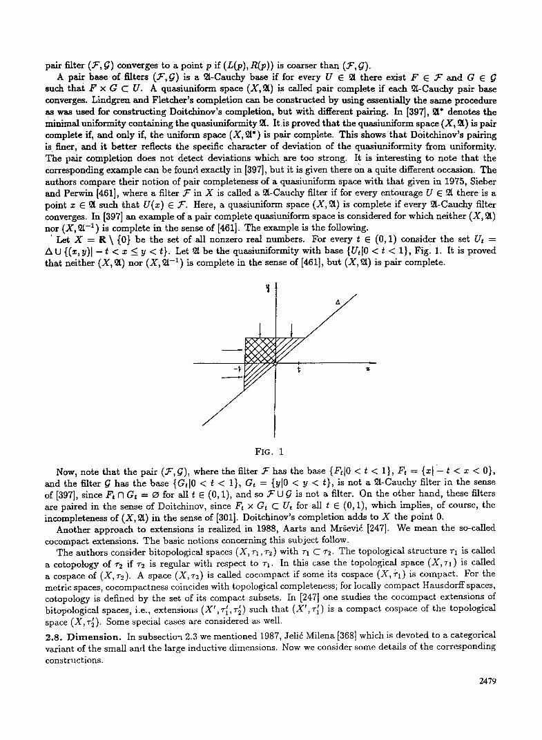
' Let X = R \ {0} be the set of all nonzero real numbers. For every ~ E (0, 1) consider the set Ut = A U {(x, Y)I - t < x _< y < t}. Let ~t be the quasiuniformity with base {Utl0 < t < 1}, Fig. 1. It is proved that neither (X, ~) nor (X, ~ - 1 ) is complete in the sense of [461], but (Z, ~) is pair complete.

, / t

FIG. 1

Now, note that the pair (~', ~), where the filter ~" has the base {F, IO < t < 1}, F, = {x I - t < x < 0), and the filter ~ has the base {Gtl0 < t < 1}, Gt = {yl0 < y < t}, is not a ~l-Cauchy filter in the sense of [397], since Ft (7 G, = ~ for all t E (0, 1), and so 3 r U ~ is not a filter. On the other hand, these filters are paired in the sense of Doitchinov, since F t x Gt C U t for all t E (0, 1), which implies, of course, the incompleteness of (X, ~/) in the sense of [301]. Doitchinov's completion adds to X the point 0.

Another approach to extensions is realized in 1988, Aarts and Mr~evid [247]. We mean the so-called cocompact extensions. The basic notions concerning this subject follow.

The authors consider bitopological spaces (X, T1, ~-2) with rl C r2. The topological structure ~-1 is called a cotopology of r2 if r2 is regular with respect to rl. In this case the topological space (X, T1 ) is called a cospace of (X, v2). A space (X,~-2) is called cocompact if some its cospace (X, 7-1) is compact. For the metric spaces, cocompactness coincides with topological completeness; for locally compact Hausdorff spaces, cotopology is defined by the set of its compact subsets. In [247] one studies the cocompact extensions of bitopological spaces, i.e., extensions (X', r~, ~-~) such that (X' , r~) is a compact cospace of the topological space (X, v~). Some special cases are considered as well.

2.8. D i m e n s i o n . In subsectioq 2.3 we mentioned 1987, Jelifi Milena [368] which is devoted to a categorical variant of the small and the large inductive dimensions. Now we consider some details of the corresponding constructions.

2479

Let E be a fixed class of bitopological spaces considered as a parameter of the theory. It is denoted in [368] by EB to emphasize that we are dealing with bitopological spaces (the category of bitopological spares and their bicontinuous mappings is usually denoted by B), A bitopological space X = (X, r l , r2) is called ~-disconnected between its subsets A and B if there exist X ~ = ( X t, ~ ri, r2) E e and a bicontinuous mapping f : X --* X ' such that the r;-closure o f / ( A ) has the empty intersection with the r '-closure of /(B),i,j=l,2, i~ j . Apair(z,F) iscalledregularifz~X, FeCriNCr2, andz~F.

A pair (F, H) is called normal if F E Crl N Cr2, H E Cri N Cr2, and F N H = ~. A subset A of a bitopological space (X, r l , r2) is called p-closed if A = F~ N F2, F I E Cry, and F2 E Cr2. A set A is called an E-separation of a regular pair (z, F) (a normal pair (F, H)) if it is p-closed in

( X , r , , v2) and X \ A is E-disconnected between x and F (between F and H). p - i ndEX = --1 (p-IndEX = - 1 ) i f X = o. p-ind E X <_ n ( k i n d EX <_ n) if for every regular pair (z, F) :(for every normal pair (F, H)) there exists

an E-separation A such that p-ind EA _< n - 1 ( k i n d EA <_ n -- 1). p-ind EX = n ( k i n d EX = n) if p-ind EX _< n ( k i n d E X <_ n) and the condition p-ind E X _< n -- 1 is

wrong (the condition p-ind EX _< n -- 1 is wrong). On the whole, this construction is parallel to the construction of small and large dimensions given in

1974, Dvalishvili [57] and in 1977, Dvalishvili [60]. The category E is used in [368] only to fix separations of regular and normal pairs. Certain initial results are given. In particular, it is noted that the both inductive dimensions p-ind E X and p-Ind EX are monotone with respect to E.

2.9 . M a n y - v a l u e d m a p p i n g s . The many-valued mappings of bitopological spaces are a natural object of study in the theory of bitopological hyperspaces (spaces of subsets) since any many-valued mapping f : X -~ Y is none other than a mapping of X into P Y = {A1A C Y}. For example, one considers lower semicontinuous many-valued mappings and upper semicontinuous many-valued mappings.

A many-valued mapping f : (X, r ) -* (X', r ' ) is called lower semicontinuous (upper semicontinuous) if for any point x0 E X and any rt-open set V having nonempty intersection with f ( xo) (containing f (zo)) there exists a r-neighborhood U of x0 such that f ( x ) N V r 0 ( f (z ) C V) for each point x e U.

Sometimes we consider mappings which are both lower and upper semicontinuous. We can consider such a mapping f : X --~ X ~ as a bicontinuous mapping of X into P X ~ with respect to a suitable choice of bitopological structures on X and P X . It is obvious that we can fix the bitopological structure (r, ~') on X. On the other hand, (Qr t, P r *) would be a suitable bitopological structure on P X f in such a situation. Here Qr ~ and P~'~ axe the topological structures on P X ~ defined at the end of subsection 2.1: their bases of open sets consist of all sets of the form QG = {AN G ~ O} and P G = {A[A C G}, respectively; G e r ' .

It is also possible to consider the many-valued mappings of bitopological spaces (including semicontinuous mappings) by passing to the corresponding bitopological structure on the set of subsets of the target bitopological space.

In 1987, Mukherjee and Ganguli [427] consider the upper (lower) almost continuous many-valued map- pings.

The corresponding definition can be given as follows. A many-valued mapping f : (X,~'l, r2) --~ (X', v~, r~) is called upper (lower) i j -almost continuous if for

any point x 0 E X and any r~-open set V having a nonempty intersection with f (xo) (containing f (xo)) there exists a ri-neighborhood U of x0 such that f ( x ) N (V"])~.~ ~ ~ (resp:, ( f ( x ) C (~V";),.~) for every point"

x E U , i , j = l , 2 , i C j . In this situation we also can pass to the mapping f : X ~ P X ~ with a suitable bitopological structure

on P X t. We see that to study many-valued mappings it is necessary to bitopologize the sets of subsets in a suitable

way.

2.10. C o n n e c t i o n wi th o t h e r s t r u c t u r e s . There are various connections between bitopological struc- tures in the sense of Kelly and other structures studied in different fields of mathematics. This includes merely using some structures for the definition of the others as well as adoption of ideas and the mutual use of results, and, what is especially important, interaction in the process of development of the corresponding theories, which results in the origin of a new direction of research.

2480

Consider the interaction of this kind of bitopological theory with the theory of quasiuniform spaces. As a matter of fact, the origin itself of the notion of a bitopological space is due to the quasimetric

spaces. As early as 1931, Wilson [239] observed that any quasiuniform structure defines two topological structures. In 1963, Kelly [98] also emphasizes that the connection between the bitopological structures and quasimetrics is a kind of basis for the new notion and the new direction of study. In reality, one can find the origins of the theory of bitopological spaces in different fields of mathematics, but, nevertheless, the theory of quasiuniform (quasimetric) spaces is its recognized primary source. For example, the bitopological and the quasiuniform approach are interwoven in the theory of extensions of bitopological spaces and in the theory of completions of quasiuniform spaces.

Among the extensions of an arbitrary bitopological space (X, r l , I-2) are those defined by the minimal open Cauchy filters of general uniform structures pl, p2 on the topological spaces (X, rl) , (X, ~'2) and a one-to-one correspondence between the pl- and the p2-Cauchy filters. In some cases, the uniform structures Pl and p2 are defined by a suitable quasiuniform structure P2 on X and the one-to-one correspondence is defined by the pairing with respect to 9/. In this way we simultaneously obtain special extensions of bitopological spaces and completions of quasiuniform spaces.

In connection with using the quasiuniform structures for construction of extensions of bitopological spaces, some problems arise, which have a definite interest both for the theory of bitopological spaces and for the theory of quasiuniform spaces.

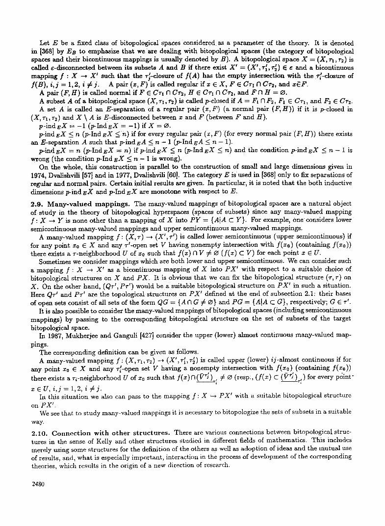
The character of these problems is well illustrated by the following example. Let X = (0, 1), and let r~ : r2 = r be the usual topology on X and d the usual metric, (x, y) = Ix - Yl.

Obviously, the completion of the metric space (X, d) is the segment [0, 1], also with the usual topology. In this case, the quasiuniform structure P2 is even a uniform structure. A base of the latter can be given graphically, see Fig. 2, where the character of decrease of the base elements is shown by the arrows.

// FIG. 2

A uniform structure ~ defines on (X, r l ) = (X, r ) and (X, r2) = ( X , r ) the same uniform structure pl = p2 = p with the base consisting of finite covers by intervals. Here we have two pl-Cauchy filters wl and w~ and two p2-Cauchy filters, the same wl and w2, not converging to the points of X. The 9/-pairing of these filters is the identical correspondence.

Now, note that the bitopological space (X, r , ~') under consideration has another extension (X ' , rI, r~). It is defined by the same filters wl,w2, but with different pairing, wl -~ w2, w2 --~ wl. One can represent this extension as the segment [0, 1] on which r I is the usual topology, but for r~ we have convergencies

(x.l e N) 1 if (x-I e N) 0, and �9 N) 7 0 if �9 N) 1.

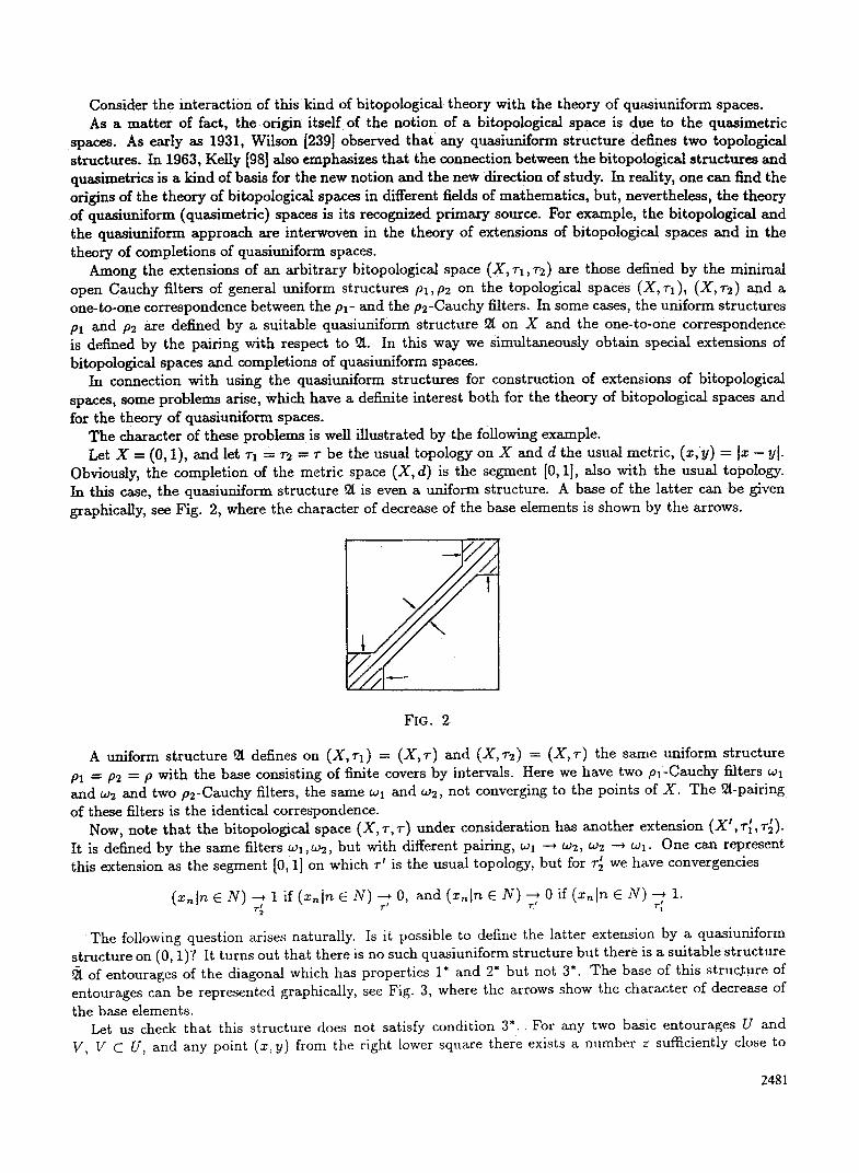
The following question arises naturally. Is it possible to define the latter extension by a quasiuniform structure on (0, 1)? It turns out that there is no such quasiuniform structure but there is a suitable structure ~ /of entourages of the diagonal which has properties 1" and 2* but not 3*. The base of this structure of entourages can be represented graphically, see Fig. 3, where the arrows show the character of decrease of

the base elements. Let us check that this structure does not satisfy condition 3*. For any two basic entourages U and

V, V C U, and any point (x, y) from the right lower square there exists a number z sufficiently close to

2481

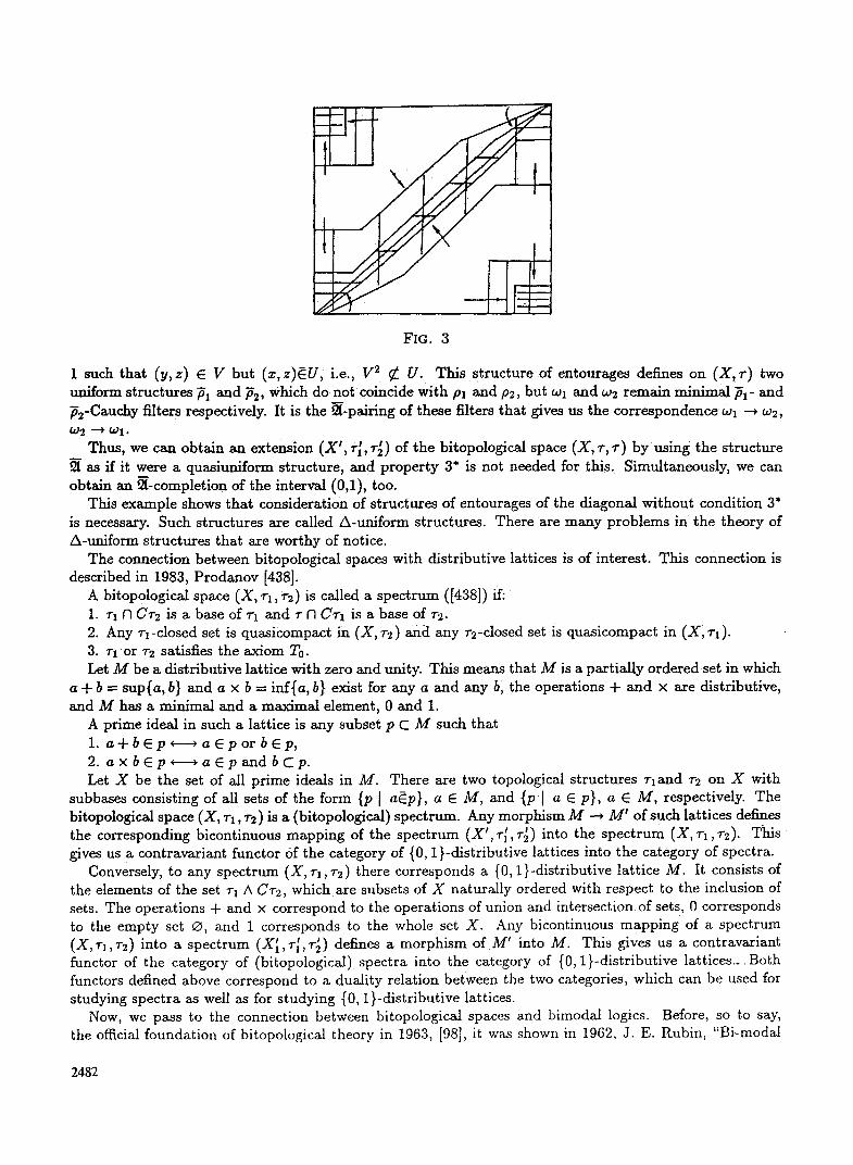
FIG. 3

1 such that (y ,z) E V but (x,z)~U, i.e., V 2 • U. This structure of entourages defines on (X,~') two uniform structures Pa and P2, which do not coincide with pl and p2, but wa and w~ remain minimal Pl- and ff2-Cauchy filters respectively. It is the ~-pairing of these filters that gaves us the correspondence wl ~ w2, t o 2 ~ t.o 1 .

Thus, we can obtain an extension (X ~, i , r i , r2) of the bitopological space (X, r, ~') by using the structure as if it were a quasiuniform structure, and property 3* is not needed for this. Simultaneously, we can

obtain an PA-completion of the interval (0,1), too. This example shows that consideration of structures of entourages of the diagonal without condition 3*

is necessary. Such structures are called A-uniform structures. There are many problems in the theory of A-uniform structures that are worthy of notice.

The connection between bitopological spaces with distributive lattices is of interest. This connection is described in 1983, Prodanov [438].

A bitopological space (X, r l , r2) is called a spectrum ([438]) if: 1. 7"1 f3 Cr2 is a base of 7"1 and r fl Ca'l is a base of vs. 2. Any rl-closed set is quasicompact in (X, 7"2) and any T2-closed set is quasicompact in (X, ~'1). 3. rl or T2 satisfies the axiom To. Let M be a distributive lattice with zero and unity. This means that M is a partially ordered set in which

a + b = sup{a, b} and a x b = inf{a, b} exist for any a and any b, the operations + and • are distributive, and M has a minimal and a maximal element, 0 and 1.

A prime ideal in such a lattice is any subset p C M such that 1. a + b E p ~ * a E p o r b E p , 2. a • * a E p a n d b C p . Let X be the set of all prime ideals in M. There are two topological structures viand r2 on X with

subbases consisting of all sets of the form {p J a~p}, a E M, and {Pl a E p}, a E M, respectively. The bitopological space (X, r l , ~'2) is a (bitopological) spectrum. Any morphism M ---* M ' of such lattices defines

I'F't Tt the corresponding bieontinuous mapping of the spectrum vL , a, ~'~) into the spectrum (X, ~-a, r2). T h i s gives us a contravariant functor of the category of {0, 1}-distributive lattices into the category of spectra.

Conversely, to any spectrum (X,~'~, r2) there corresponds a (0, 1}-distributive lattice M. It consists of the elements of the set ~'x A C~-2, which axe subsets of X naturally ordered with respect to the inclusion of sets. The operations + and • correspond to the operations of union and intersection of sets, 0 corresponds to the empty set ~, and 1 corresponds to the whole set X. Any bicontinuous mapping of a spectrum (X,T, ,r2) into a spectrum (XI,~'[,r~) defines a morphism of M' into M. This gives us a contravariant functor of the category of (bitopologicM) spectra into the category of (0, 1}-distributive lattices... Both functors defined above correspond to a duality relation between the two categories, which can be used for studying spectra as well as for studying {0, 1}-distributive lattices.

Now, we pass to the connection between bitopological spaces and bimodai logics. Before, so to say, the official foundation of bitopological theory in 1963, [98], it was shown in 1962, J. E. Rubin, "Bi-modal

2482

logic, double-closure algebras artd Hilbert space," Zeitchr. f/ir Math., 8, 305-322, that to any bimodal logic we can assign a bitopological space just in the same way as we assign a topological space to any modal logic. The system $24 has two modal connectives 01 and 02, the strict and the weak possibilities. For any propositional variable p we have the relation 01 p -'* 02 p between them. The strong and the weak necessities l-ll and l'12 are defined as -,, 01 "" q and ,-~ 02 "~ q, respectively, where ,-, is the connective of negation and tr is an arbitrary tame formula. When constructing a bitopological model of a bimodal logic we assign a subset of some fixed set X to each propositional variable, the complement to the negation, the intersection to the conjunction, the union to the disjunction, the closures to the connectives 01 and (>2, and the interiors to the connectives O1 and 02. The axioms of the bimodal logic 5'24 are such that the two closure operations define two topological structures vx and rz, r2 C ri. In general, there exist different bimodal logics, and we assign to them different types of bitopological spaces. The axiomatics of a logic defines the axiomatics of the corresponding bitopological space, and vice versa. This interrelation makes possible a simultaneous s tudy of the bimodal logics and the bitopological spaces.

It is known that the connectives 01 and 0 can be interpreted as possibilities in the past and in the future, but it seems more natural to interpret them as two different individuals' viewpoints on the possibility. Such an approach allows us to pass to n-modal logics (n > 2) and naturally raises the problem of adjusting the modal logics of different individuals and creating their common modal logic, and so on.

There are different generalizations of the notion of topological space. One of them is the notion of r-space (J. Zuzgak, "Generalized topological spaces," Math. Slovaka, 33, 249 (1983)). A pair (X, 79) is an r-space if :D C P X and the following conditions are 511filled:

1. ~ E 7 9 , X E 7 9 . 2. For any A C X and B E :D, B C A, there exists a maximal element C E D such that B C C C A. The sets belonging to 79 are called open in (X, 79). A maximal set C C A open in (X, 79) is called the

interior of A. Since �9 E 79, any A has an interior which is not uniquely defined in the general case. It is clear that any topological space is an r-space. In 1988, Fukutake [331] noted that (X, vx U 7"2) is an r-space for any bitopological space (X, vl, r2). In the same paper, the connections between separations in r-spaces and separations in bitopological spaces are considered.

2.11. Fuzzy b l t o p o l o g i c a l spaces . The theory of fuzzy sets and systems is very advanced and has a vast literature. Its specialists kre united in an international association with its own periodical edition "Fuzzy Sets and Systems." The theory of fuzzy topological spaces and the theory of (usual) bitopological spaces arose nearly simaltaneously, but only in recent years the fuzzy bitopological spaces at t racted some attention.

The notion of a fuzzy set is, of course, the initial notion of the theory of fuzzy sets and systems. By a fuzzy subset of a set X one usually calls any mapping #: X ~ [0, 1]. The set of all fuzzy sets in X is denoted by I x . In particular, the usual (accurate) sets correspond to the mappings #A: X --~ {0, 1} with pA(Z) = 1 if z e A, and t.tA(X) = 0 if x~A. The empty set is denoted by 0, 0(z) = 0 for all x e X, and the set X itself is denoted by 1, l (x) = 1 for all x E X.

The relation of inclusion is defined for the fuzzy sets, namely

#i < P 2 if / z l ( x ) < p 2 ( x ) for all x e X .

The operations of union, intersection, and complement are also defined:

( U / z ~ ) ( z ) = s u p # ~ ( x ) , ( N # ~ ) ( x ) = i n f ~ t ~ ( z ) , ( C # ) ( z ) = l - ~ t ( z ) . o t o t

o~ o t

All these definitions agree with the definitions of inclusion, union, intersection, and complement for usual

sets. Similar to the usual topological structure, a fuzzy topological structure 7- on X can be defined as a subset

v C f x satisfying the usual axioms. On the other hand, we can increase the degree of fuzziness by defining a topological structure on X as a mapping r : I x ~ I such that the corresponding conditions are fulfilled. For example, one can require that

.r(U,al ) >_ sup~-(tzc,), V(#l f3#2) >_ min{7-(/zl),7-(kt2)}, v(0) = 7-(1)---- 1. t i t

6Y

2483

The notion of a fuzzy bitopological space like that of a fuzzy topological space appears to have a proba- bilistic character. Let us say that the mapping/~: X --* I corresponds to fuzzy set A~,. Then the number g(z) can be considered as the probability of the event z E A. Thus, the events x E A and their probabilities /~(z) are defined. However, we have neither a whole space of events nor, more importantly, an unambigu- ously defined probabilistic measure on it, i.e., we have no random set. A fuzzy set is a badly truncated random set.

In this connection let us consider the following example. Let D = {0, 1}, ~: D ~ I , ~b(0) = ~b(1) = �89 One can consider the mapping ~b as a fuzzy set Ar The event 0 E Ar is the complex event (Ar = {0}) V(Ar = {0, 1}, and, similarly, the event 1 E Ar is the complex event (A,~ = {1})V(Ar = {0, 1}). The numbers ~(0) and ~b(1) can be considered as the probabilities of these complex events. In our example they are equal to �89 But this leaves unknown the probabilities of the elementary events (Ar = ~), (A~, = {0}), (Ar = {1}), and (A~ = {0, }). These events constitute a complete system of pairwise incompatible elementary events, which generate the corresponding space of events. The probabilistic measure on this space is defined by fixing the probabilities pl , p2, p3, and p, of realization of these four elementary events in the indicated order. By fixing the mapping ~ we fix two relations, namely

p~ + p, = r p, + p, = ~(1) .

Under our assumption ~b(0) = ~b(1) = �89 these relations together with pz + p2 + p3 + p4 = 1 imply the equations

1 1 Pl ----/)4, P2 -~ ~ --/)4, P3 ~- ~ -- P4,

where P4 < �89 and p4 is arbitrary in all other respects. Thus, there is a continuum of random subsets of the set D that correspond to one and the same fuzzy set.

Let us continue the study of our example. It seems quite natural to define the operations of union, intersection, and complement for fuzzy sets so

that they would agree with ~the corresponding operations for random sets. The following example shows that in reality it is not so.

Consider two random sets in D,

1 1 A : pl = 0, p~ = p~ = 7 ' p* = 0; A ' : p~ = p~ = p~ = p~ = ~.

These random sets define one and the same fuzzy set A~ = A,~, because

1 ~ b ( 0 ) = p 2 + p 4 = l , 9(1) =p3 + p , = l , ~ ' ( 0 ) = p ~ + p ~ = l , ~ b ' ( 1 ) = p ~ + p ~ = 2 .

By definition of the union of two fuzzy sets we have AO UAr A6, where ~(0) = max{~b(0), ~'(0)} - I

1 Now consider the union A U A' = / i of random sets, where pl, p2, p3, and ~(1) = m ~ { r r = ~. and P4 denote the probabilities of the elementary events defining/i . A simple calculation shows that in the general case

Pl = P l P~, t t

P2 = PlP2 q- PiP2 -4- P2P2,

P3 =plp~TP~P3-}-P3P~, I l l I l l !

P4 = PlP~ 4- PiP4 q- P2P3 + PzP3 + P2P4 q- P3P4 4- P3P4 q- P4P4,

and in our special case we obtain

1 1 1 A : ~ , = O , ~ = ~ , ~ 3 = ~ , ~ = ~ -

2484

This implies ~(0) = s = 3 X # ~, and so

We see that the operation of union of fuzzy sets does not agree with the operation of union of random sets. This means that the notion of fuzzy set has no clear semantics. Nevertheless, the theory of fuzzy spaces (topological or bitopological) contains many results. Strictly speaking, the whole (hi)topological theory can be made fuzzy automatically, although there will be certain deviations, to be sure. For example, for a usual subset A of X we have the relation A U C x A = X , while for a random set A this is not true, as a rule. As a consequence, the usual proof of the compactness of a closed subset in a compact space does not work for fuzzy spaces.

Here we consider only one paper, in which the peculiarities of the fuzzy theory become more apparent than in the others. This is 1989, Abd E1-Monsef and Ramadan [249]. By a fuzzy topological space they call a subset r C I X satisfying the usual axioms, and by a fuzzy bitopological space, a set with two fuzzy topological structures.

A system w of fuzzy subsets of a set X is called an o~-cover if for any point x E X there exists an A~, E w such that ~(x) > o~. This notion allows us to formulate different versions of o~-compactness of fuzzy bitopological spaces, which are parallel to the corresponding versions of compactness of usual bitopological spaces. For example, it is known that the notion of FHP-compactness, K-compactness, and KN-compactness are equivalent. At the same time, it is proved in [249] that after passing to the corresponding s-variants only the first and the second version remain equivalent. In this connection we can suggest the following improvement of the idea of s-compactness, where the number ~ is not fixed.

A system w of fuzzy subsets of a set X is called its F-cover if there exists an e > 0 such that for every point x E X there is A~, E w with #(x) > e. Using this notion, one can state different versions of the notion of F-compactness.

In [249], one also considers different versions of compactness, which have the usual fuzzy-theoretical nature, as well as the connections between them.

w 3. GENERAL THEORY OF BITOPOLOGICAL SPACES

3.1. In recent years, the development of the system of essentially bitopologicai notions was continued. Some of them arose outside bitopological theory but proved to be interesting for this theory, too. First of all, consider the notions connected with the diagonal.

Klaas Pieter Hart, "Spaces for which the diagonal has a closed neighborhood," Colloq. Math., 8, 49- 56 (1987) considers the notion of A-normality of a topological space. He calls a topological space (X, r) A-normal if the diagonal A has a closed base of neighborhoods in (X • X, r • r). This notion admits a natural generalization to the notion of A-normality of a bitopological space.

A bitopological space (X, fl) is called A-normal if the diagonal A has a closed base of neighborhoods in ( x x x , f l ) .

Every local bitopological space is A-normal because each neighborhood of the diagonal is closed in ( x x

A. Css General Topology, Adem Hilder Ltd., Bristol (1978) considers the notion of a divisible topological space. A topological space (X, r) is divisible if every neighborhood U of the diagonal A in (X x X, r x r) contains a subneighborhood V such that V 2 C U. This notion has the following generalization.

A bitopological space (X, fl) is called A-divisible if every neighborhood U of the diagonal A in (X x X, fl) contains a subneighborhood V such that V 2 C U, in other words, if the set of all neighborhoods of the diagonal generates a quasiuniform structure.

In 1972, Fletcher and Lindgren [321] consider the notion of transitive quasiuniformity. A quasiuniformity on X is called transitive if each entourage U contains an entourage V such that V 2 -- U. This notion is

associated with localization of the familiar notion of transitivity of a bitopological space, see [91]. - * (x, y) We remind the reader that a bitopological space (X, fl) is transitive if the convergences (xx, yx) /~

--+ (x, z). The following is the localization of this and (yx,zx) --~ (y, z) imply the convergence (za, zx)

notion.

2485

A bitopological space (X, 8) is called locally transitive if the convergences (xx, yx) ~ (x ,x) and (yx, zx) 7

(z,x) imply the convergence (zx, zx) 7 (x,z) .

It is easy to see that the A-transitivity implies the local transitivity but the converse is not true. The condition of local transitivity is much weaker than that of A-transitivity.

One way or the other, each of these notions is related with neighborhoods of the diagonal. Therefore, it is natural to consider the structure 92 consisting of all the neighborhoods of the diagonal in- (X x X, 8). This is obviously a A-uniform structure on X. We denote it by A fl and say that the A-uniform space (X, Aft) and the bitopological space (X , /3 ) are mutually compatible (the A-uniform structure A 8 and the bitopological structure 8 are compatible).

To every bicontinuous mapping 9 : (X, fl) ~ (X',8') there corresponds a uniform mapping A ~ : (X, A/5) ~ (X', A8') . Thus, we obtain a covariant functor

A : Bitop -* A Uaif

of the category of bitopological spaces and bicontinuous mappings to the category of A-uniform spaces and uniform mappings.

By se t t ing(X, B') < (X, 8) (or fl' < 8) if the identical mapping i: (X, 8) ~ (X, 8 ') is bicontinuous (i.e., fl' C/~) we introduce an order relation on the set of all bitopological spaces (bitopological structures) compatible with a fixed A-uniform space X. This set is nonempty and, in general, has neither maximal nor minimal element.

In fact, let 92 be a A-uniform structure on X. Then 80 = 92 U {0} is a topological structure on X x X, i.e., r0 is a bitopological structure on X compatible with 92, Ari0 = 92. Now, note that

8.={GIGnac{x},GcXxX}

also is a bitopological structure on X compatible with 92 for an arbitrarily fixed x E X. Let /5 be a bitopological structure on X such that r= C f l for all z E X. Then for any G C X • we have G = U G ~ I x E X w h e r e

G = (G \ u (G n E c #,

and, therefore, G E #. But this means that fl = P(X x X) is the discrete bitopologicM structure and Ari consists of all subsets of X x X tha t contain A.

Now, consider a bitopological structure 8 which is contained in r0 = 92 U {~} and compatible with 92. The structure/~ must consist of the empty set and (not necessary all) elements of 92. These sets constitute a base of 92 in the sense that every entourage of A contains an entourage which is open in (X x X, 8).

Assume that 8 contains two certain sets G1 and G2, X x X # G2 C G1 # ft. Consider the bitopological s t ruc tu re# ' ----(SAG1)U{X x X } C ft. G2Eri' since G2 # X x X and G2EflAG1. Thus, 8 strictly contains/~' . Therefore, the minimal bitopological structure compatible with 92 must consist of three sets only, namely ~ , G, and X x X. Hence, G must be the minimal element of the A-uniform structure ~ , possibly coinciding with X x X.

Note that if the minimal element of A-uniform structure 92 is the diagonal, then 92 consists of all subsets of X x X containing A, and the minimal bitopological structure compatible with 92 consists of the sets O, A, X x X. This is the only case when there is both a minimal and a maximal element among all the bitopologicai structures compatible with 92.

The functor A: Bitop ---* A Unif is a natural basis for the simultaneous study of bitopological and A- uniform structures. On the other hand, one can also consider the tautological functor/3o : A Unif ~ Bitop such that ri0(X, 92) = (X, ri0(92)) and (fl0 qo)(x) = 79 (x) for qa: (x, 92) -~ (X', 92').

Since Aft0 : A Unif ---* A Unif is the identical functor, the category Bitop is an enrichment of the category A Unif [347, 349], r0 is an embedding of A Unif into Bitop, and ~x is a covering of A Unif by Bitop.

2486

3.2. The bitopological structure/30 = ~ U {~} is defined for any A-uniform structure ~. Considered as a topological s t ructure on X x X, this structure induces a trivial topological structure on the diagonal. The bitopological structures fl that are trivial on A are characterized by the following property: if G E/~ and G N A # ~, then 2~ C G.

Among the bitopological structures that are trivial on A and compatible with an arbitrarily fixed A- uniform structure ~ there is no minimal structure in general, but there always is a maximal one. This is the bitopological structure/~1 = ~t (92) defined as follows: G E fll if and only if G N A = O or G E ~ (see [358], p. 45). The structure fl~ is always a local bitopological structure.

It is known that for any bitopological structure/~, of interest is the system {~(z, ) , f l( , y) I x �9 X, y E X} of traces of fl on all vertical and horizontal sets {x} x X and X x {y} in X x X. A trace is the topological structure Z(x, ) (fl(, y)) induced by fl on the corresponding vertical (horizontal) set. It is easy to give an example when different bitopological structures define the same system of traces. In this connection the locally decomposable bitopological structures should be noted, which exist only for the so-called continuous system of traces and not for an arbitrary one (see [358], pp. 47-48), but on the other hand such a structure is uniquely defined by the corresponding system.

For any A-uniform structure 92, we can consider the bitopological s t ruc ture /~ = fl~ (92) defined by it and the corresponding system of traces {fl~(x, ), i l l( , y)}. If the latter is continuous, consider the corresponding locally decomposable bitopological structure fit(P.t). Thus, to every A-,mlform structure 92 with a continuous system of traces there corresponds a uniquely defined local, locally decomposable bitopological structure fit. It easy to see that different A-uniform structures can define the same locally decomposable bitopotogical structure.

We say that a system of traces

), Z( ,v) Ix �9 x , y �9 x }

is vertically totally continuous if the convergences

- _ - _ +

#(,y)

imply the convergence ((z~, y~) l/z E M) - -* (z, y).

a(,v)

Here M is the directed ordered set of pairs (~, h) where ~ E E, h: .--. --* A, A = UA, I ~ E .~., h(~) E Ar We set h < h' if there exists ~0 E -~- such that h(~) = h'(~) for ~ < ~0 and h(~0) < h'(~0), (~, h) < (~', h') if

< ~' or ~ = ~' but h < h', x~ = zh(~),/z = (~, h). Note that the definition of vertical total continuity differs from that of vertical continuity only by the

fact that the convergence ((x, I e z) (x, v)

is not required. Thus, the condition of vertical total continuity is stronger than that of vertical continuity. The notion

of horizontal total continuity of a system of traces is defined similarly. A system of traces is called totally continuous if it is vertically and, at the same time, horizontally totally

continuous. Consider an arbitrary A-uniform structure ~ with totally continuous system of traces. Then we can

define a decomposable bitopological structure f la = r l x 7"2 on X by setting (xx } .k E A) --* z iff ((xx, x)) I

�9 A) and �9 A) x iff I �9

The total continuity condition guarantees that the topological structures rl and r2 are well defined. Thus, to any A-uniform structure 92 with a totally continuous system of traces we can assign a uniquely

defined decomposable bitopological structure fla.

2487

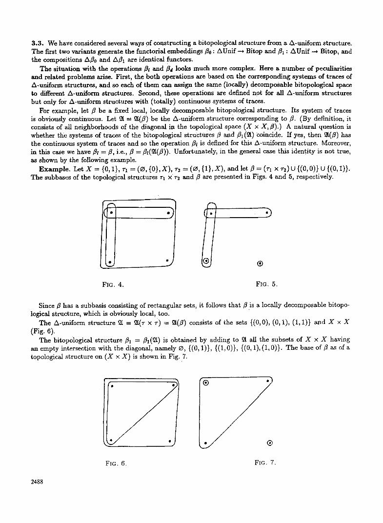
3.3. We have considered several ways of constructing a bitopological structure from a A-uniform structure. The first two variants generate the functorial embeddings fl0 : AUnif --* Bitop and/~1 : AUnif --* Bitop, and the compositions Aft0 and A/~I are identical functors.

The situation with the operations/31 and ~,r looks much more complex. Here a number of peculiarities and related problems arise. First, the both operations are based on the corresponding systems of traces of A-uniform structures, and so each of them can assign the same (locally) decomposable bitopological space to different A-uniform structures. Second, these operations are defined not for all A-uni form structures but only for A-uniform structures with (totally) continuous systems of traces.

For example, let /3 be a fixed local, locally decomposable bitopological structure. Its system of traces is obviously continuous. Let 92 = 92(fl) be the A-uniform structure corresponding to /~. (By definition, it consists of all neighborhoods of the diagonal in the topological space (X x X,/~).) A natura l question is whether the systems of traces of the bitopological s t ructures/3 and fl~ (92) coincide. If yes, then 92(fl) has the continuous system of traces and so the operation fit is defined for this A-uniform structure. Moreover, in this case we have/3t = ~, i.e.,/~ =/~!(92(/~))- Unfortunately, in the general case this identi ty is not true, as shown by the following example.

E x a m p l e . Let X = {0, 1}, rl = (~, {0}, X), r2 = (0 , {1}, Z ) , and let fl = (rl x r2) U {(0, 0)} U {(0, 1)}. The subbases of the topological structures rl x r~ and fl are presented in Figs. 4 and 5, respectively.

�9 2 : J

.)

|

FIG. 4. FIG. 5.

Since/~ has a subbasis consisting of rectangular sets, it follows tha t /3 is a locally decomposable bitopo- logical structure, which is obviously local, too.

The A-uniform structure 92 = 92(r x r ) = 92(/~) consists of the sets {(0, 0), (0, 1), (1,1)} and Z x Z (Fig. 6).

The bitopological structure/~1 = fl1(92) is obtained by adding to 92 all the subsets of X • X having an empty intersection with the diagonal, namely ~, {(0, I)}, {(1, 0)}, {(0, 1), (1, 0)}. The base of fl as of a topological s t ructure on (X x X) is shown in Fig. 7.

(e e- r|

j

FIG. 6. FIG. 7.

2488

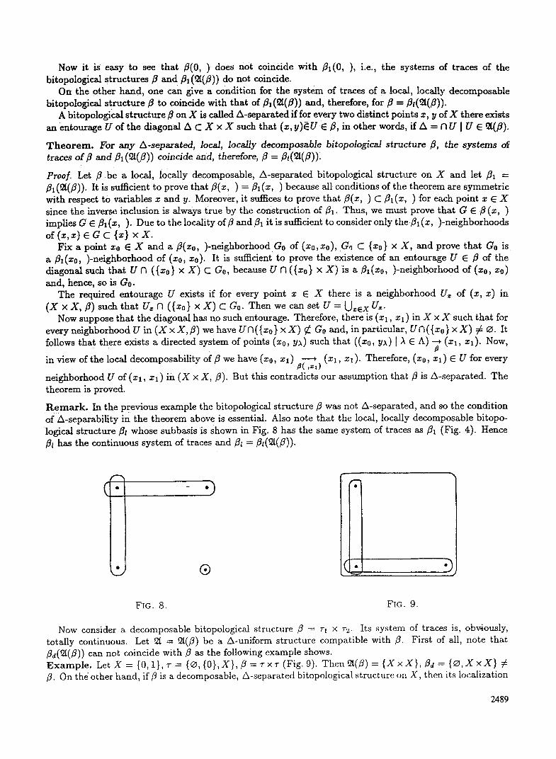
Now it is easy to see that #(0, ) does not coincide with ill(0, ), i.e., the systems of traces of the bitopological structures fl and fll (~i(~)) do not coincide.

On the other hand, one can give a condition for the system of traces of a local, locally decomposable bitopological s t ructure fl to coincide with that of fll(~i(fl)) and, therefore, for ~ = flt(~t(fl)).

A bitopological structure/~ on X is called A-separated if for every two distinct points z, y of X there exists an entourage U of the diagonal A C X x X such that (x, y)~U E fl, in other words, if A = f3 U ] U E ~(fl).

T h e o r e m . For any A-separated, local, locally decomposable bitopologicM structure ~, the systems of traces o f # and fl1(~(fl)) coincide and, therefore, # = #,(~(fl)):

Proof. Let fl be a local, locally decomposable, A-separated bitopological s tructure on X and let fll = fll (~(fl)). It is sufficient to prove that fl(x, ) = fll ( x , ) because all conditions of the t h e o r e m are s y m m e t r i c with respect to variables x and y. Moreover, it suffices to prove that fl(z, ) C fl~ ( x , ) for each point z E X since the inverse inclusion is always true by the construction of ill. Thus, we must prove that G E fl(x, ) implies G E ill(x, ). Due to the locality offl and fl~ it is sufficient to consider only thefl~ (x, )-neighborhoods of e a c x x .

Fix a point x0 E X and a fl(Zo, )-neighborhood Go of (xo,xo), Go C {x0} x X, and prove tha t Go is a ~l(x0, )-neighborhood of (x0, x0). It is sufficient to prove the existence of an entourage U E fl of the diagonal such tha t U f3 ({x0} x X) C Go, because U n ({x0} x X) is a fll(Xo, )-neighborhood of (x0, x0) and, hence, so is Go:

The required entourage U exists if for every point x E X there is a neighborhood U~ of (x, x) in (X x X, #) such that U~ N ({x0} x X) C Go. Then we can set U = [J~Ex U~.

Now suppose that the diagonal has no such entourage. Therefore, there is (xt, xl ) in X x X such that for every neighborhood V in ( Z x X, fl) we have UN({x0} x X) ~ Go and, in particular, UN({x0 } x X) ~t ~. It follows that there exists a directed system of points (x0, y~) such that ((x0, y~) [ A E A) --+ (xl, zl) . Now, # in view of the local decomposabili ty of fl we have (x0, Xl) #(,--~) (xl , xl ). Therefore, (x0, x,) E U for every

neighborhood U of (x~, Xl) in (X x X, fl). But this contradicts our assumption that fl is A-separated. The theorem is proved.

R e m a r k . In the previous example the bitopological s tructure fl was not A-separated, and so the condition of A-separability in the theorem above is essential. Also note that the local, locally decomposable bitopo- logical structure fit whose subbasis is shown in Fig. 8 has the same system of traces as fll (Fig. 4). Hence fl~ has the continuous system of traces and flz = flt(~(fl)).

I

�9 | ( - .)

FIG. 8. FIG. 9.

Now consider a decomposable bitopological structure /3 = 7"i • ~-2- Its system of traces is, obviously, totally continuous. Let 9/ = 9/(fl) be a A-uniform structure compatible with ft. First of all, note that #a(9/(#)) can not coincide wi th # as the following example shows. E x a m p l e . Let X = {0, 1}, r = {~D, {0},X}, fl = Tx~- (Fig. 9). Then 9.1(fl) = { X x X } , fla = { ~ , X x X } # ft. On the other hand, if fl is a decomposable, A-separated bitopological structure on X, then its localization

2489

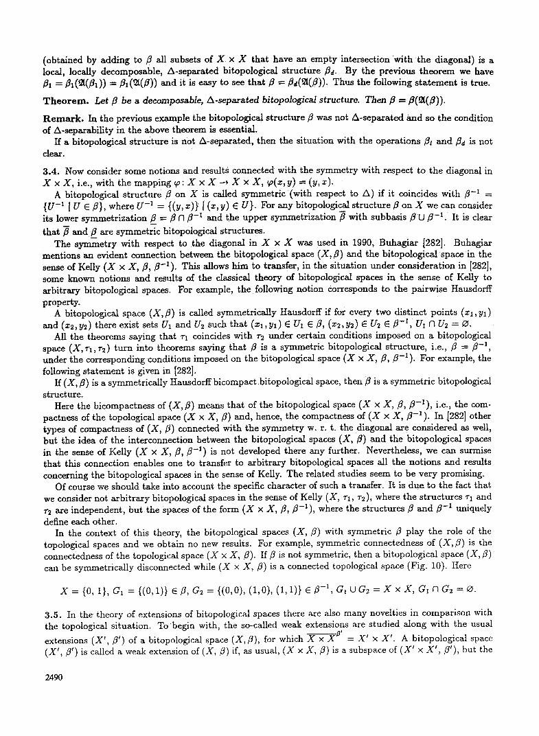
(obtained by adding to fl all subsets of X x X that have an empty intersection with the diagonal) is a local, locally decomposable, A-separated bitopological s t ructure rid. By the previous theorem we have fll = f l l (~(f l l )) = f lI(~(fl)) and it is easy to see that fl -" fld(P2(fl)). Thus the following s ta tement is true.

T h e o r e m . Let fl be a decomposable, A-separated bitopological structure. Then fl = f l(~(f l)) .

R e m a r k . In the previous example the bitopological s t ructure fl was not A-separated and so the condition of A-separability in the above theorem is essential.

If a bitopological s t ructure is not A-separated, then the si tuation with the operations fll and fld is not clear.

3.4. Now consider some notions and results connected with the symmetry with respect to the diagonal in X x X, i.e., with the mapping to : X x X ~ X • X, to(x, y) = (y, x).

A bitopological s tructure fl on X is called symmetric (with respect to A) if it coincides with fl-1 = {U -1 [ U E fl}, where U -1 = {(y, x)) I (x, y) E U}. For any bitopological s tructure fl on X we can consider its lower symmetrizat ion fl_ = fl N fl-1 and the upper symmetrizat ion B with subbasis/~ U fl-1. It is clear that fl and fl_ are symmetric bitopological structures.

The symmetry with respect to the diagonal in X x X was used in 1990, Buhagiar [282]. Buhagiar mentions an evident connection between the bitopological space (X,~) and the bitopological space in the sense of Kelly (X x X, fl, ~-1). This allows h im to transfer, in the situation under consideration in [282], some known notions and results of the classical theory of bitopological spaces in the sense of Kelly to arbitrary bitopological spaces. For example, the following notion corresponds to the pairwise Hausdorff property.

A bitopological space (X, fl) is called symmetrically Ifausdorff if for every two distinct points (x~, yl) and (x2,y2) there exist sets Ua and U2 such that (xa,ya) e U1 e fl, (x~,y2) e U2 E f l -x , UI n U2 = 0.

All the theorems saying that ~'1 coincides with r2 under certain conditions imposed on a bitopological space (X, rl,l"2) turn into theorems saying that ~ is a symmetric bitopological structure, i.e., ~ = / 3 -1, under the corresponding conditions imposed on the bitopological space (X x X, /~, /~-1) . For example, the following s ta tement is given in [282].

If (X, fl) is a symmetrically Hausdorff bicompact bitopological space, then/3 is a symmetr ic bitopological structure.

Here the bicompactness of (X, fl) means that of the bitopological space (X x X, /~, fl-~), i.e., the com- pactness of the topological space (X x X, fl) and, hence, the compactness of (X • X, #-~ ). In [282] other types of compactness of ( X , fl) connected with the symmetry w. r. t. the diagonal are considered as well, but the idea of the interconnection between the bitopological spaces (X, ~) and the bitopological spaces in the sense of Kelly (X x X, fl, #-1) is not developed there any further. Nevertheless, we can surmise that this connection enables one to transfer to arbitrary bitopological spaces all the notions and results concerning the bitopological spaces in the sense of Kelly. The related studies seem to be very promising.

Of course we should take into account the specific character of such a transfer. It is d u e to the fact that we consider not arbitrary bitopological spaces in the sense of Kelly (X, ~'1, r2), where the structures rl and 7"2 are independent, but the spaces of the form (X x X, fl, fl-1), where the structures fl and fl-1 uniquely define each other.

In the context of this theory, the bitopological spaces (X, ~) with symmetric ~ play the role of the topological spaces and we obtain no new results. For example, symmetric connectedness of (X, ~) is the connectedness of the topological space (X x X, fl). If ~ is not symmetric, then a bitopological space (X,/3) can be symmetrically disconnected while (X x X,/~) is a connected topological space (Fig. 10). Here

x = {o, 1}, a , = {(o, e Z, = {(o,o), (1,o), (1,1)} e Z - ' , c , = x • a , =

3.5. In the theory of extensions of bitopological spaces there are also many novelties in comparison with the topological situation. To begin with, the so-called weak extensions are s tud ied along with the usual

extensions (X ' , ~') of a bitopological space (X, fl), for which X x XZ' = X' x X' . A bitopological space (X' , /3 ' ) is called a weak extension of (X,/3) if, as usual, (X x X, fl) is a subspace of (X' x X ' , fl'), but the

2490

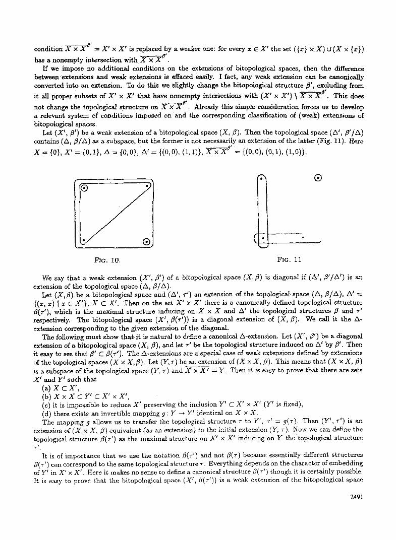
condition X x Xg ' = X ' x X ' is replaced by a weaker one: for every z E X ' the set ({z} • X ) U ( X x {z})

has a nonempty intersection with X x ~a', If we impose no additional conditions on the extensions of bitopological spaces, then the difference

between extensions and weak extensions is effaced easily. I fact, any weak extension can be canonically converted into an extension. To do this we slightly change the bitopological structure fl~, excluding from

it all proper subsets of X ' x X ' that have nonempty intersections with (X ' x X') \ -X---ff--X/J'. This does

not change the topological s tructure on X • Already this simple consideration forces us to develop a relevant system of conditions imposed on and the corresponding classification of (weak) extensions of bitopological spaces.

Let (X ' , #') be a weak extension of a bitopological space (X,/~). Then the topological space (A' , # ' / A ) contains (A, # / ~ ) as a subspace, but the former is not necessarily an extension of the latter (Fig. 11). Here

X = {0}, X ' = {0, 1}, A = {0,0}, A ' = {(0,0), ( I , I ) ) , X x X #' = {(0,0), (0,1), (1,0)}.

?

FIG. 10. FIG. 11

We say that a weak extension (X', d') of a bitopo2ogical pace (X, #) is diagon 1 if (a' , # ' / a ' ) is an extension of the topological space (A, f l /A).

Let (X, #) be a bitopological space and (A', f ' ) an extension of the topological space (A, # / A ) , &' = {(z, z) I z E X'} , X C X' . Then on the set X ' • X ' there is a canonically defined topological structure /~(r'), which is the maximal structure inducing on X • X and A' the topological structures fl and r ' respectively. The bitopological space (X', fl(r ')) is a diagonal extension of (X, #). We call it the A- extension corresponding to the given extension of the diagonal.

The following must show that it is natural to define a canonical A-extension. Let (X ' , fl') be a diagonal extension of a bitopological space (X, fl), and let r ' be the topological structure induced on A' by fl'. Then it easy to see ~hat fl' C fl(r ') . The/h-extensions are a special case of weak extensions defined by extensions of the topological spaces (X x X, #). Let (II, r ) be an extension of (X x X, fl). This means that (X • X, #) is a subspace of the topological space (Y, ~') and X x X ~ = Y. Then it is easy to prove that there are sets X ' and Y' such that

(a) x c x ' , (b) X x X C Y' C X ' x X' , (c) it is impossible to reduce X ' preserving the inclusion Y' C X' x X' (Y' is fixed), (d) there exists an invertible mapping g: Y --~ Y' identical on X x X. The mapping g allows us to transfer the topological structure ~- to Y', ~-' = 9(~'). Then (Yf, ~-') is an

extension of (X x X~ ~) equivalent (as an extension) to ~he ini~iM extens}on (I/, r). Now we can define the topological structure fl(r ') as the maximal structure on X ~ x X ~ inducing on Y the �9 structure T f"

It is of importance that we use the notation B(r') and not /~(r) because essentially different structures B(r ~) can correspond to the same topological structure r. Everything depends on the character of embedding of Y~ in X' x X'. Here it makes no sense to define a canonical structure fl(r ') though it is certainly possible. It is easy to prove that the bitopological space (X', ~t(r')) is a weak extension of the bitopological space

2491

(X,/~). Significantly different weak extensions (X ' , /~ ( r ' ) ) of (X, fl) can correspond to the same extension (Y, r ) of the topological space (X x X, ~/). The study of such extensions appears to b e an interesting problem.

w 4. BITOPOLOGICAL REPRESENTATIONS OF CLASSES OF MAPPINGS

4.1. We say that a class B of bitopological structures gives a bitopological representation of a class ~" of continuous mapping of topological spaces if ~" coincides with the class of all bicontinuous mappings f: (X,/3) ~ (X',/3'), where fl, fit are all the possible dements of B.

Since any bitopological structure is in fact a topological structure, a bitopological representation of the given class ~" gives us its topological description. Sometimes, however, one has to consider not arbitrary continuous mappings but those from a well-described class .,4. Then we obtain a bitopological description of ~" in the class ,4. Let us give an example of such a description.

T h e o r e m . Let (X, r) be a connected topological space and let qo: (X, r) --~ (X, 7-) be a continuous mapping without fixed points. Then the set of the continuous mappings of the space (X, r) into itself that are permutable with cp has a bitopologicad representation in the class of one-to-one mappings.

Proof. L e t / ~ be a topological structure on X x X such that (a) if U l r~, = ~, then U 6/~n C fl~, (b)/9 I r~ = ~- x ~ I r~. Let f : (X, fl~) -~ (X,/~,) be a bicontinuous mapping. Then f x f : (X x X, fl~) --~ (X x X,/~,) is a

continuous mapping. Since F~, is the only connected component in (X x X, fl~), either (f x f)F~ C F~ or (f x f)(F~) is a single-point set. But the second case drops out since f is one-to-one. Let x be a point of X , (x,~o(x)) 6 F~. Then ( f x f ) (x , qo(x)) = ( f (x) , l ip (x ) ) 6 r~ and so f ~ ( x ) = qvf(x) , i.e., the mapping f is permutable with ~v. Then ( f x f ) ( z , ~(z)) = ( f ( z ) , f ~ ( z ) ) = ( f (z ) , ~ f ( z ) ) E F~.

Now consider a continuous mapping f : (X, v) -* (X, v) permutable with ~o. Since all one-point subsets of X x X not belonging to F~, are open in (X x X,/~w), the continuity of f x f follows from that of ( f x f ) I I'~. But the latter is obvious because/~ I~= v x v I F~ and ( f x f ) (F~) C F~.

4.2. Now, let r be a set of continuous mappings of a topological space (X, r ) into itself. Consider the system (F~ I ~ 6 O) of subsets of X x X, where F~ is the graph of the mapping qo: (X, v) -+ (X, 7-). On every set F~ C X x X we fix the topological structure fl~, = v x r I F~,. We introduce on X x X a topological structure j8r by letting U 6/~r if and only if U n F~, 6 ~8~ for every mapping ~ 6 O.

A continuous mapping r (X, r ) --* (X, v) is called a 0-mapping if the mapping I x r (X, r ) --* ( X x X , 1~r ) is continuous.

L e m m a . Each mapping 7~ 6 �9 is a O-mapping.

Proof. We have (1 x ~)(X) C F~, since (1 x ~)(x) = (x, W(x)) E F~ for every x 6 X. Then the mapping I x ~: (X,7-) --~ (X x X, fie) is continuous s ince /~ = ~" x r [ F~, and so ~ is a @mapping.

A set �9 of continuous mappings of (X, 7-) into itself is called bitopologically complete if every O-mapping belongs to O.

T h e o r e m . / f �9 is a bitopo10gically complete system of continuous mappings ~: (X, 7-) --* ( X 7-), then the homeomorhism r : (X, 7-) ~ (X, 7-) is a bicontinuous mapping of (X, ~r onto itself if and only if ~bqvr -1 E �9 for aI1qa E O.

Proof. Let ~b be a homeomorphism (X, 7-) onto itself and let r ~v ~b -~ E �9 for all q~ E O. Let (x, y) 6 F~, i.e., let y = ~o(x). Then (r x r = (~b(x),ip'r where ~0' = r 1 6 2 6 O. Thus (r x r C C~,. Since/3~ = 7- x 7- I F~ and/3~, = 7- x 7- I Fv,', it follows that (~ x ~b) I F~ is a continuous mapping for all ~oEO.

Now consider V E/3, , U = (r x r Then U 6/3r since U F1 F V, = ((r x r -1 (V FI F~,) E/3~ for every ~o E ~. This proves the continuity of the mapping r x ~b or, what is the same, the bicontinuity of the mapping r (X, f l , ) ~ (X, /3r

2492

Now let ~b be a homeomorphism of (X, r ) onto itself which is a bicontinuous mapping (X, fl~) onto itself. The mapping ~b -1 is a continuous mapping of (X, r ) onto itself. Let ~a E (~. Then the mapping

x ~a: (X, r ) ~ (X x X, ]~ ) is continuous by the previous lemma. But then the composition (~b x ~)(1 x ~o)~ - l = 1 x ~b ~a ~b -~ also is a continuous mapping of (X, r ) into (X • X, fl~), i.e., ~b ~a ~b -~ is a 4~-mapping. Hence, in view of the bitopological completeness of ~, we have ~b ~a ~b -1 E ~.

R e m a r k . We can interpret the condition ~b ~a ~b - l E ~ as the permutability of ~b and ~ (~b �9 = ~ ~b). Then the above theorem can be stated as a theorem on bitopological representation, namely:

If ~ is a bitopologically complete system of continuous mappings of a topological space (X, r ) into itself, then the set of all homeomorhismsof (X, v) onto itself permutable with �9 has a bitopological representation.

4.3. The problem of a bitopological representation o f the set of all differentiable (piecewise-differentiable) mappings R m --* R n as well as of different classes of such mappings has long at tracted the attention of the specialists, although without considerable progress. Here we also restrict ourselves only by mappings of R -* R of the real line and try to make it clear how and what results can be obtained in this direction.

We consider the following type of topological structures /3 on R • R. These are local bitopological structures defined by the convergences

((s (= + - to) 7 (s(=),

with the usual topological structure on the diagonal of R x R. Here x is an arbitrary real number, f an arbitrary function in a fixed class of differentiable functions which is closed with respect to the composition. It is clear that for every such f the mapping f : (X, fl) --* (X,/3) is bicontinuous.

If a bitopological structure/3 on R is constructed based on the set of all differentiable functions, then we can choose a function which has no derivative at x = 0, but nevertheless maps (R, ~) to (R,/3) bicontinuously. Thus,/3 is not a bitopological representation of the set of all differentiable functions on R.

If we limit ourselves by the set of differentiable functions with nonvanishing derivatives, then the cor- responding bitopological structure gives its bitopological representation. The same can be said about the set of all diffeomorphisms of R with the only difference that we obtain a bitopological representation in the class of mappings of R onto itself. On this way one can obtain some other results as weU.

One can suggest another way of bitopologizing the real line, which has a direct relation to the problem of a bitopological representation for differentiable functions. Here the bitopological structure is also local but not compatible with the usual bitopological structure on R: there are no convergent sequences in (R x R,/3) at all except the diagonal ones (on the diagonal we have the usual topology). In this case the existence of derivative of function f at point x depends on the fact of whether (x, x) is a limit point of the set ( f x f)(A), where A is a suitable set having x as a limit point in the usual topology.

w 5. BITOPOLOGICAL MANIFOLDS AND BITOPOLOGICAL GROUPS

5.1. It is known [358] that the study of a sequential bitopological structure on fl,( can be reduced to the study of germs of converging sequences. Here we suggest another method of s tudy of (rid, fl) which makes use of nonstandard calculus.

Nonstandard calculus starts with the introduction of a nonstandard real line *R containing the real line R. The field *R is, of course, a non-Archimedean extension of the ordered field R, and it is always possible to construct a non-Archimedean calculus on *R. But not every non-Archimedean extension of a real line is suitable for constructing nonstandard calculus. It is necessary that the so-called transfer principle be applicable to *R. The essence of this principle can be stated as follows.

Consider a theory 92 on calculus: for example, the Contents of a certain textbook. This theory contains notions, definitions, statements, and arguments concerning the real line R. Then the transfer principle says that this theory can be interpreted as a theory *92 consisting of the corresponding notions, definitions, statements, and arguments, this time concerning *R. The true statements of the theory *92 correspond to the true statements of the theory 92, and vice versa.

2493

Consider some examples of using the transfer principle. Let 2t contain the notion of natural numbers and that of the set N C R of all natural numbers. Then *~i also contains the notion of natural numbers and the notion of the set *N C* R of all natural numbers. Further, if ~ makes use of the induction principle "if A C N, 1 E A, n E A imply n + 1 E A, then A = N," then in *~l we can use the corresponding induction principle "if A C TV', 1 E A, n E A imply n + 1 E A, then A = ~rV'."

The theory *~t will be a duplicate, an exact copy, of the theory 2t having, however, another base: *N instead of R. The passage from ~t to *~ by itself gives nothing new, but later on it yields an essentially nonstandard extension of the theory *~, which is impossible to obtain on the s tandard level by extending the theory 92 itself.

For example, the notion of infinitesimal is essentially nonstandard. A number a E *R is cMled infinitesi- mal if [o~[ < a for every positive number a E R. This notion is not contained in the theory *P/for any theory 9 /on R. It can not be obtained by using the transfer principle in spite of the fact that in usual calculus there is a notion of infinitesimal sequence.

Recall that a sequence (xk [ k E N) in R is called infinitesimal if for each e > 0 there is k0 E N such that [xt,[ < e for k >_ k0. The use of the transfer principle gives us the sequence (xk [ k E *N) in *R and not an infinitesimal number in *R.

Nevertheless, by a suitable choice of the nonstandard real line *R we can pass from infinitesimal sequences in R to infinitesimals in *R, although this procedure has no relation to the transfer principle. In turn, this allows us to pass from a convergence (x/, I k E N) ~ x in R to a number x + a E *R, where a is the infinitesimal in *R corresponding to the infinitesimal sequence (xt, - x I k E N). The next step is the transition from convergences (xk I k E N) --+ x in R n to points (vectors) x + a C *R n, where a = ( a l , a 2 , . . �9 an) is a vector with infinitesimal components. If two convergences (xk I k e N) ~ x and (x~ I k E N) ---* x belong to the same germ, then a = a ' , i.e., every germ of a convergence defines a unique point in *R. For a fixed x E R" this point x q- a E* R n is uniquely defined by a E *R~, where * ~ is the set of all infinitesimal vectors (i.e., vectors with infinitesimal components).

Now consider a fiber space R" • *R~' with base R n and fiber *R~. Every point x q- a E *R'* defines a point (x, a) of this space, and translation of germs convergent in R'* determines translation (x, a) ~ (y, fl) of points. Thus the bitopological structure fl on R n is defined by the fiber space R n • *R~ with a translation relation fixed on it.

5.2. Now turn to the problem of bitopologization of groups. In [358] different approaches to the notion of a bitopological group were described, cf. 1987, Cfiznpian and Cs [286]. A bitopological group is defined as a group G endowed with a bitopological structure fl such that the mappings

m: ( a x G, --. ( a x a , m ( . , y) = y- ' . ) ,

;: ( a x a , #) --, ( a x a , = y- ' ) ,

are continuous. Of all the definitions of bitopological group suggested at different times, none has an obvious advantage

and each one has essential deficiencies. Compare these variants. In [18] a group G with two topological structures rl and r2 is called a bitopological group if the cor-

respondence ( x , y ) ~ x y is a bicontinuous mapping of (G x G, rl x rl , 7-2 x r2) into (G, T1, 7.2) and the correspondence x --* x -1 is a homeomorphism of (G, r l) onto (G, ~'2).

However, it is easily seen that, in fact, a bitopological group (G, ~q, r2) in the sense of [18] is determined by fixing on G only one topological structure rl such that the mapping

p: (G x G, 7"1 X 7"1) -'-4 ( a , T1), p ( Z , y ) = xy

is continuous. Really, the topological structure v2 is obviously defined by the topological structure rl, namely

r2 = ra -~ = { G -~ I G E T1 }, G -1 : { x -1 I z E a } -

On the other hand, if xoyo = z0 E W -1 E 7.2, then yo 1Xo I = Zo 1 E W E rl, and by the continuity of the mapping p: (G • G,v~ x 71) ~ (G, 7.~) there are U E 7.1 and V E 7"1 such that Xo ~ E U, yo ~ E V, and

2494

f l ( V x U ) C W. But t h e n z 0 E U -1 E r z , y0 E V -1 E r2, a n d p ( U -1 x V -1) C W -1 i.e., the mapping p( • • G, r2 x r2) --* (a , r2) is continuous.

Thus, the not ion of a bitopological group in the sense of [18] is obta ined from the not ion of a topological group by simply rejecting the condi t ion tha t the correspondence x --, x - I be continuous. It is not a bitopological not ion at all.

In [358] a bitopologieal group is a group G with a bitopological s t ructure fl such tha t the mappings

p: (a x a, (•, I G), p(x,y) = w

q: (a, I a) (a, BIG), = . - '

are continuous (recall tha t fl [ G is the topological s t ructure on G induced by the topological s t ructure fl on G x G under embedding j : G ---* G x G j (x ) = (x, x)).

Consider the special case fl = r l x rz of a decomposable bitopological s tructure. In this case r = fl [ O = max{r1, r~. }.

The topological s t ruc ture fl induces on G the topological s t ructures rl and ra under the embeddings j l : G ~ G • G, j l ( z ) = (x, l a ) , and jz: G ~ G • G, j2(x) = ( l a , x). Hence, the mappings

j l : (G, r l ) --+ (G x G, fl) and j2: (G, r2) -+ (G x G, fl)

are continuous. Therefore, the mappings

P j l : (G, rl)--+ (G,r ) and pj2: (G, r2)--+ (G,r )

are continuous. It follows tha t

r = m a x { r ~ , r 2 } c r ~ a n d r = m a x I q , r ~ } C r 2 ,

and so r = rl = r l . This shows tha t the not ion of a bitopological group given in [358] has an essential defect, namely, there

is no bitopological group in the sense of [358] such tha t fl = r~ x r2 and rl ~ r2. The notion of a bitopological group given in [286] has the same defect, as the authors themselves note. In [358] one more version of the not ion of a bitopological group is considered. A bitopological group is

defined as a triple (X, fl, r ) , where O is a group, fl is a bitopological s t ructure on G, and r is a topological s t ructure on G such tha t the mappings

p: (G x G, fl) --+ (G,r) , p ( x , y ) = zy and q: (G,r) --+ ( a , r ) , q(x) = x -1

axe continuous. This is a na tura l generalization of the not ion of topological group. It is obta ined by passage from r x r to an arbi t rary bitopological s t ructure ft.

Actually, in 1965, Husain Takdir [86] implicit ly uses this concept of bitopological group. He defined the so-called semitopological groups for which the condit ion of continuity of p: (G x G, r x r ) ~ ( G , r ) was replaced by tha t of continuity of p on every horizontal set G x {y} and every vertical set {x} x G ( t h e continuity of q is not required, either, but this is inessential for us now).

The condition tha t p be separately continuous in each variable x and ! /can be replaced by an equivalent condition of continuity of the mapping p: (G x G,/3) --+ (G, r) under a suitable choice of the bitopological s t ructure fl on G. One can take as fl the topological s t ructure on G x G for which a set F is closed if and only if its intersections with horizontal and vertical sets are closed in the topology induced by r x r on these sets. The mapping p: (G x G, fl) --* ( G , r ) is continuous with respect to such ft. In fact, let H be a closed set in ( G , r ) and let F = p- I (H) . Then for any horizontal or vertical set A in G x G, the set p - I ( H ) VIA = (p I A ) -1 (H) is closed in ( A , r x r I A), because of the continui ty o f p I A. But then, by the definition of fl, the set F is closed in (G x G, fl), which precisely means the cont inui ty of p: (G x G, fl) -+ (G,r) .

2495

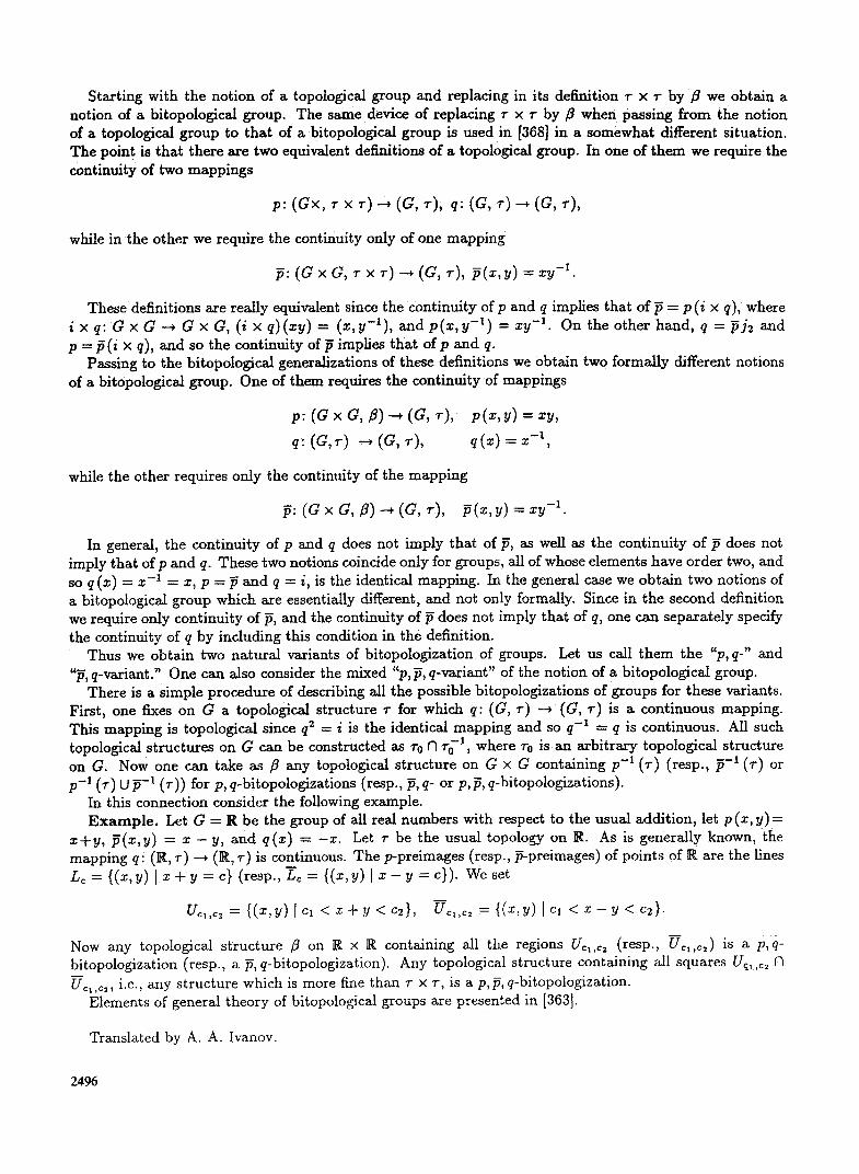
Starting with the notion of a topological group and replacing in its definition r x r by fl we obtain a notion of a bitopological group. The same device of replacing r x r by/~ when passing from the notion Of a topological group to that of a bitopological group is used in [368] in a somewhat different situation, The point is that there are two equivalent definitions of a topological group. In one of them we require the continuity of two mappings

p: (Gx, 7 x 7") -~ ((7, ~'), q: (G, I") --* (G, "r),

while in the other we require the continuity only of one mapping

These definitions are really equivalent since the continuity of p and q implies that of p = p (i • q), where i x q : G x G - - * G x G , ( i x q ) ( x y ) = ( x , y - X ) , a n d p ( x , y - 1 ) = z y -1. On the other hand, q = ~ j 2 and p = p ( i x q), and so the continuity o f ~ implies that o f p and q.

Passing to the bitopological generalizations of these definitions we obtain two formally different notions of a bitopological group. One of them requires the continuity of mappings

p : ( a x a , Z ) - - , ( a , , - ) ,

q: (G, q(z) = x -1,

while the other requires only the continuity of the mapping

~ : ( a x a , 8 ) - ~ ( a , r ) , ~ ( x , y ) = z y - ~ .

In general, the continuity of p and q does not imply that of p, as well as the continuity of ~ does not imply that of p and q. These two notions coincide only for groups, all of whose elements have order two, and so q (x) = x -1 = x, p = ~ and q -- i, is the identical mapping. In the general case we obtain two notions of a bitopological group which are essentially different, and not only formally. Since in the second definition we require only continuity of p, and the continuity of ~ does not imply that of q, one can separately specify the continuity of q by including this condition in the definition.

Thus we obtain two natural variants of bitopologization of groups. Let us call them the "p, q-" and "~, q-variant." One can also consider the mixed "p,~,q-variant" of the notion of a bitopological group.

There is a simple procedure of describing all the possible bitopologizations of groups for these variants. First, one fixes on G a topological structure r for which q: (G, r ) --* (G, v) is a continuous mapping. This mapping is topological since q2 = i is the identical mapping and so q-X = q is continuous. All such topological structures on G can be constructed as "r0 Cl r0 "-1, where 7"0 is an arbitrary topological structure on G. Now one can take as fl any topological structure on G x G containing p-1 ('r) (resp., p-1 (v) or p-1 (r) 13 ~-1 (r)) for p, q-bitopologizations (resp., ~, q- or p, p, q-bitopologizations).

In this connection consider the following example. E x a m p l e . Let G = R be the group of all real numbers with respect to the usual addition, let p (z, y) =

z- t -y , ~ ( x , y ) = x - y, and q ( x ) = - x . Let r be the usual topology on R. As is generally known, the mapping q: (R, T) ---* (R, r ) is continuous. The p-preimages (resp., ~-preimages) of points of R are the lines Lc = {(x,y) [ x q- y = c} (resp., Le = {(x,y) [ x - y = c}). We set

m

={(x,y)[cl <z+y<c2} , ={(x,y) lcl

Now any topological structure /3 on R x R containing all the regions Uc~,c2 (resp., Ur is a p,q- bitopologization (resp., a fi, q-bitopologization). Any topological structure Containing all squares U~I,~ ~ VI Ur ,~2, i.e., any structure which is more fine than 7- x v, is a p, ~, q-bitopologization.

Elements of general theory of bitopological groups are presented in [363].

Translated by A. A. Ivanov.

2496