Voltage feed welding transformer at no-load BOGOMIR ZIDARIČ PETER KOKELJ

TECES, Gosposvetska cesta 84, SI2000,Maribor

SLOVENIA

MIRKO KELEČ Indramat elektromotorji d. o. o., Kidričeva 81,

SI4220 Škofja Loka, SLOVENIA

TOMAŽ SOBOČAN Univerza v Ljubljani, Fakulteta za

elektrotehniko Tržaška 25, SI1000 Ljubljana

SLOVENIA

Univerza v Ljubljani, Fakulteta za elektrotehniko

Tržaška 25, SI1000 Ljubljana SLOVENIA

http://www.fe.uni-lj.si/staff

DAMIJAN MILJAVEC Univerza v Ljubljani, Fakulteta za

elektrotehniko Tržaška 25, SI1000 Ljubljana

SLOVENIAhttp://www.fe.uni-lj.si/staff

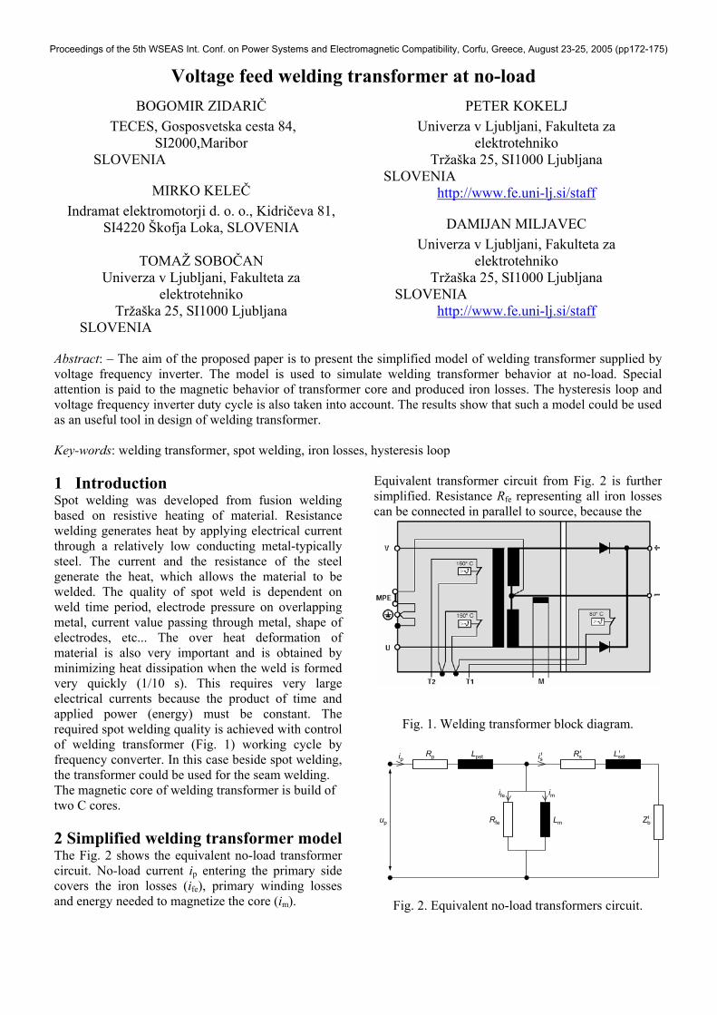
Abstract: – The aim of the proposed paper is to present the simplified model of welding transformer supplied by voltage frequency inverter. The model is used to simulate welding transformer behavior at no-load. Special attention is paid to the magnetic behavior of transformer core and produced iron losses. The hysteresis loop and voltage frequency inverter duty cycle is also taken into account. The results show that such a model could be used as an useful tool in design of welding transformer. Key-words: welding transformer, spot welding, iron losses, hysteresis loop 1 Introduction Spot welding was developed from fusion welding based on resistive heating of material. Resistance welding generates heat by applying electrical current through a relatively low conducting metal-typically steel. The current and the resistance of the steel generate the heat, which allows the material to be welded. The quality of spot weld is dependent on weld time period, electrode pressure on overlapping metal, current value passing through metal, shape of electrodes, etc... The over heat deformation of material is also very important and is obtained by minimizing heat dissipation when the weld is formed very quickly (1/10 s). This requires very large electrical currents because the product of time and applied power (energy) must be constant. The required spot welding quality is achieved with control of welding transformer (Fig. 1) working cycle by frequency converter. In this case beside spot welding, the transformer could be used for the seam welding. The magnetic core of welding transformer is build of two C cores. 2 Simplified welding transformer model The Fig. 2 shows the equivalent no-load transformer circuit. No-load current ip entering the primary side covers the iron losses (ife), primary winding losses and energy needed to magnetize the core (im).

Equivalent transformer circuit from Fig. 2 is further simplified. Resistance Rfe representing all iron losses can be connected in parallel to source, because the

Fig. 1. Welding transformer block diagram.

ip is

ife im

Rp Lpst LsstRs

Rfe Lm Zbup

Fig. 2. Equivalent no-load transformers circuit.

Proceedings of the 5th WSEAS Int. Conf. on Power Systems and Electromagnetic Compatibility, Corfu, Greece, August 23-25, 2005 (pp172-175)

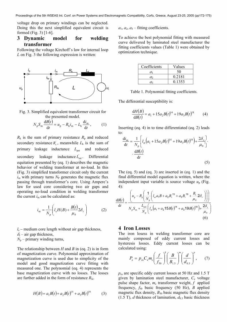
voltage drop on primary windings can be neglected. Doing this the next simplified equivalent circuit is formed (Fig. 3) [1-6]. 3 Dynamic model for welding

transformer Following the voltage Kirchoff`s law for internal loop L on Fig. 3 the following expression is written:

ip im

ife

LkRk

Rfeup uiL

Fig. 3. Simplified equivalent transformer circuit for the presented model.

( )t

iLiRuttBSN

dd

dd m

kmkpmp −−= , (1)

Rk is the sum of primary resistance Rp and reduced secondary resistance '

sR , meanwhile Lk is the sum of primary leakage inductance pstL and reduced

secondary leakage inductance 'sstL . Differential

equitation presented by (eq. 1) describes the magnetic behavior of welding transformer at no-load. In this (Fig. 3) simplified transformer circuit only the current im with primary turns NP generates the magnetic flux passing through transformer’s core. Using Ampere’s law for used core considering two air gaps and operating no-load condition in welding transformer the current im can be calculated as:

( )

+= r

0s

pm 2)(1 δ

µtBBHl

Ni (2)

ls – medium core length without air gap thickness, δr – air gap thickness, Np – primary winding turns, The relationship between H and B in (eq. 2) is in form of magnetization curve. Polynomial approximation of magnetization curve is used due to simplicity of the model and good magnetization curve fitting with measured one. The polynomial (eq. 4) represents the base magnetization curve with no losses. The losses are further added in the form of resistance Rfe. ( ) ( ) ( ) ( )19

315

21 tBatBatBaBH ++= (3)

a1, a2, a3 – fitting coefficients. To achieve the best polynomial fitting with measured curve delivered by laminated steel manufacturer the fitting coefficients values (Table 1) were obtained by optimization technique.

Coefficients Values a1 50 a2 0.2181 a3 0.1353

Table 1. Polynomial fitting coefficients.

The differential susceptibility is:

( )( ) ( ) ( )18

314

21 1915d

d tBatBaatBBH

++= (4)

Inserting (eq. 4) in to time differentiated (eq. 2) leads to:

( ) ( )( )( )ttB

tBatBaalNt

i

dd

219151d

d

0

r183

1421sr

p

m

⋅

⋅

+++=µδ

(5) The (eq. 5) and (eq. 3) are inserted in (eq. 1) and the final differential model equation is written, where the independent input variable is source voltage up (Fig. 4):

( )

( ) ( )( )

++++

+++−

=

0

rsr

p

pstmp

0

ttsr

ppp

dd

µδ

δµ

21915

21

183

1421

193

1521

tBatBaalNL

SN

BBaBaBal

NRu

ttB

rt

(6) 4 Iron Losses The iron losess in welding transformer core are mainly composed of eddy current losses and hysteresis losses. Eddy current losses can be calculated using:

,3.05.150

ceese

pmk

dd

BB

ffmCpP

= (7)

pes are specific eddy current losses at 50 Hz and 1.5 T given by lamination steel manufacturer, Ce voltage pulse shape factor, mc transformer weight, f applied frequency, f50 basic frequency (50 Hz), B applied magnetic flux density, B50 basic magnetic flux density (1.5 T), d thickness of lamination, d0.3 basic thickness

Proceedings of the 5th WSEAS Int. Conf. on Power Systems and Electromagnetic Compatibility, Corfu, Greece, August 23-25, 2005 (pp172-175)

(0.3 mm) and k, m, p are material dependant exponents. For hysteresis losses calculation stands:

,5.150

chhsh

n

BB

ffmCpP

= (8)

phs are specific hysteresis losses at 50 Hz and 1.5 T given by lamination steel manufacturer, Ch voltage pulse shape factor and n is material dependant exponent. The total iron losses can be found using: hefe PPP += . (9) In table 2 there are presented all used parameter values for iron losses calculation and the results of computation.

pes [W/kg]

Ce mc [kg]

f [Hz]

B [T]

0.4 1.4 3.2 1000 1 d

[mm] k m p phs

[W/kg] 0.1 2 1.8 1.6 0.8 Ch n Pe

[W] Ph

[W] Pfe [W]

1.4 1.8 62 35 97

Table 2 Values of used parameters and iron losses results.

The value of resistance Rfe, representing hysteresis and eddy current losses, depends on used laminated steel (quality, thickness…) and inverter duty cycle kd. To calculate Rfe (eq. 11) for different inverter duty cycle kd the reference value Rfe-ref (eq. 11) is calculated for 30% reference duty cycle kd-ref. These data are provided from manufacturer for losses on unit volume of used steel (Table 2).

( )Ω=

⋅⋅== 1336

973,056022 2

fe

d_refapfe_ref P

kuR (10)

2

d

d_reffe_reffe

=

kk

RR (11)

5 Results The dynamic model equitation (eq. 6) is numerically solved using Runge-Kutta method. To get the hysteresis loop the calculation of magnetic field is done using:

( )

( )

,2

sr

0pp

t l

tBNitH

δµ

−= (12)

ip is total no-load current:

mp iRu

ife

p += . (13)

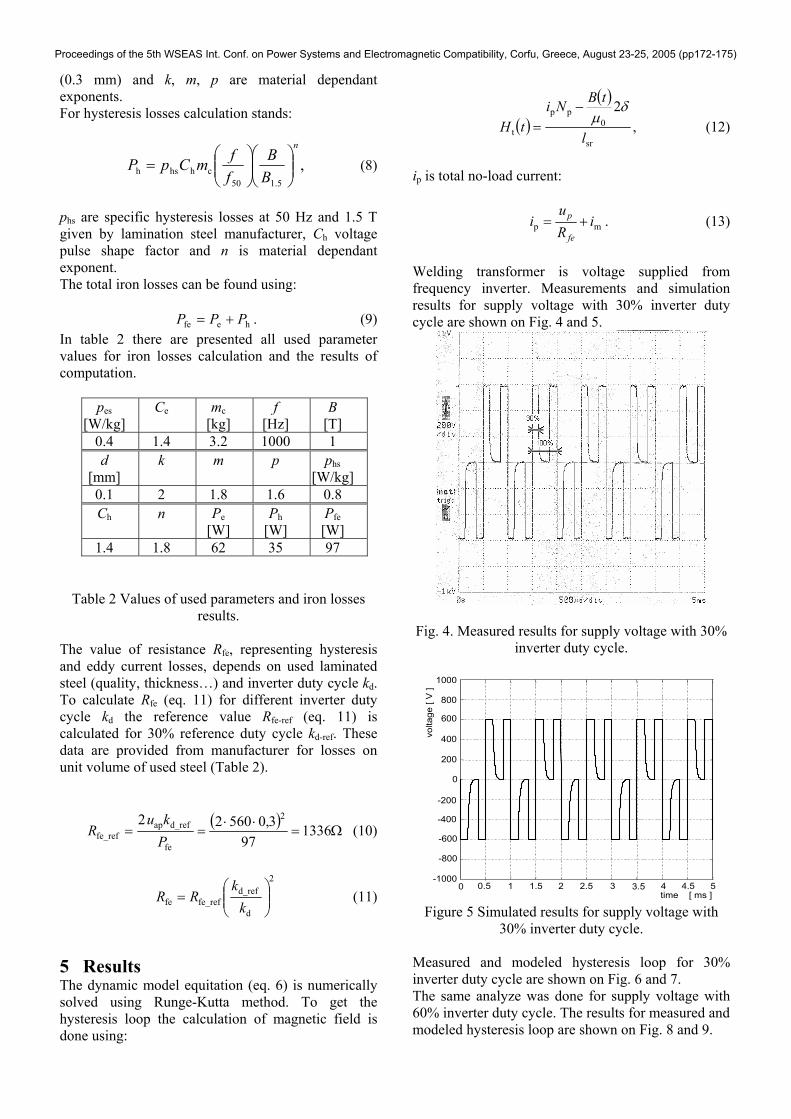
Welding transformer is voltage supplied from frequency inverter. Measurements and simulation results for supply voltage with 30% inverter duty cycle are shown on Fig. 4 and 5.

Fig. 4. Measured results for supply voltage with 30%

inverter duty cycle.

time [ ms ]

volta

ge [

V ]

0 0.5 1 1.5 2 2.5 3 3.5 4 4.5 5

1000

800

600

400

200

0

-200

-400

-600

-800

-1000

Figure 5 Simulated results for supply voltage with

30% inverter duty cycle. Measured and modeled hysteresis loop for 30% inverter duty cycle are shown on Fig. 6 and 7. The same analyze was done for supply voltage with 60% inverter duty cycle. The results for measured and modeled hysteresis loop are shown on Fig. 8 and 9.

Proceedings of the 5th WSEAS Int. Conf. on Power Systems and Electromagnetic Compatibility, Corfu, Greece, August 23-25, 2005 (pp172-175)

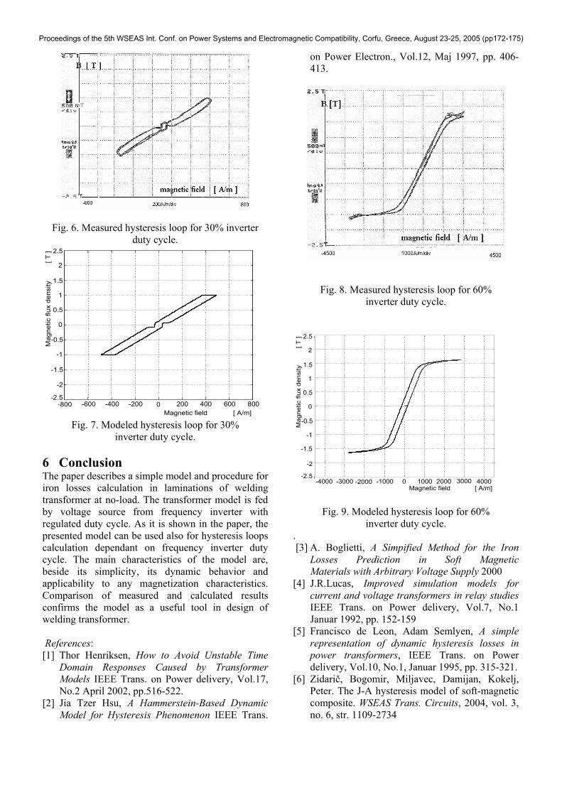
Fig. 6. Measured hysteresis loop for 30% inverter duty cycle.

-800 -600 -400 -200 0 200 400 600 800

2.5

2

1.5

1

0.5

0

-0.5

-1

-1.5

-2

-2.5

Magnetic field [ A/m]

Mag

netic

flux

den

sity

[ T

]

Fig. 7. Modeled hysteresis loop for 30%

inverter duty cycle. 6 Conclusion The paper describes a simple model and procedure for iron losses calculation in laminations of welding transformer at no-load. The transformer model is fed by voltage source from frequency inverter with regulated duty cycle. As it is shown in the paper, the presented model can be used also for hysteresis loops calculation dependant on frequency inverter duty cycle. The main characteristics of the model are, beside its simplicity, its dynamic behavior and applicability to any magnetization characteristics. Comparison of measured and calculated results confirms the model as a useful tool in design of welding transformer. References: [1] Thor Henriksen, How to Avoid Unstable Time

Domain Responses Caused by Transformer Models IEEE Trans. on Power delivery, Vol.17, No.2 April 2002, pp.516-522.

[2] Jia Tzer Hsu, A Hammerstein-Based Dynamic Model for Hysteresis Phenomenon IEEE Trans.

on Power Electron., Vol.12, Maj 1997, pp. 406-413.

Fig. 8. Measured hysteresis loop for 60% inverter duty cycle.

-4000 -3000 -2000 -1000 0 1000 2000 3000 4000

2.5

2

1.5

1

0.5

0

-0.5

-1

-2

-2.5

Mag

netic

flux

den

sity

[ T

]

-1.5

Magnetic field [ A/m]

Fig. 9. Modeled hysteresis loop for 60% inverter duty cycle.

. [3] A. Boglietti, A Simpified Method for the Iron

Losses Prediction in Soft Magnetic Materials with Arbitrary Voltage Supply 2000

[4] J.R.Lucas, Improved simulation models for current and voltage transformers in relay studies IEEE Trans. on Power delivery, Vol.7, No.1 Januar 1992, pp. 152-159

[5] Francisco de Leon, Adam Semlyen, A simple representation of dynamic hysteresis losses in power transformers, IEEE Trans. on Power delivery, Vol.10, No.1, Januar 1995, pp. 315-321.

[6] Zidarič, Bogomir, Miljavec, Damijan, Kokelj, Peter. The J-A hysteresis model of soft-magnetic composite. WSEAS Trans. Circuits, 2004, vol. 3, no. 6, str. 1109-2734

Proceedings of the 5th WSEAS Int. Conf. on Power Systems and Electromagnetic Compatibility, Corfu, Greece, August 23-25, 2005 (pp172-175)