i

Proceedings of the Mexican Optics and Photonics Meeting (MOPM2015)

2015 Academia Mexicana de Óptica www.amo-ac.mx Editors Amalia Martínez García Eric Rosas Oracio Barbosa

ii

Preface This volume contains the refereed contributions that were presented at the 2015 special edition of the Mexican Optics and Photonics Meeting, which was co-organized with the Centro de Investigaciones en Óptica on the occasion of its XXXV anniversary; and took place in the city of León, Mexico, on September 9 to 11, 2015. The Mexican Optics and Photonics Meeting is a consolidated three-days-long conference organized every two years by the Academia Mexicana de Óptica, also the Mexico Territorial Committee for Optics of the International Commission for Optics, in partnership with the Mexican public research centers together with the public and private higher education institutions; designed to provide the Mexican optics and photonics community´s recent outstanding research results with international visibility. This year the Mexican Optics and Photonics Meeting 2015 served as the central activity in the celebration of the “International Year of Light and Light-based Technologies, 2015” by the Mexican optics and photonics community, and which included the IX Symposium “Optics in Industry”, collocated with the V International Symposium of Experimental Mechanics, co-organized with the Society of Experimental Mechanics and the Centro de Investigaciones en Óptica; the 2015 Active Learning in Optics and Photonics workshop, co-organized with the Instituto Investigación en Comunicación Óptica of the Universidad Autónoma de San Luis Potosí; the international school “Light in Science, Light in Life, 2015”, co-organized with the Instituto de Física of the Universidad Nacional Autónoma de México; among many other all around the country. The 2015 special edition of the Mexican Optics and Photonics Meeting received several internationally recognized speakers such as professors William E. Moerner, 2014 Nobel laureate in chemistry; Yasuhiko Arakawa, 2014-2017 President of the International Commission for Optics, Pedro Andrés, 2013-2016 President of the Red Iberoamericana de Óptica; Eric Mazur, 2015 Vice President of The Optical Society; Toyohiko Yatagai, 2015 President of The International Society for Optics and Photonics; Zeev Zalevsky, 2008 ICO Prize laureate; and Chandra Shakher, 2014 ICO Galileo Galilei Prize laureate. As organizers we wish to thank the authors, presenters, and session chairs for their contributions, participation and support to all the above mentioned symposia, particularly to the Mexican Optics and Photonics Meeting 2015.

Amalia Martínez Eric Rosas

Oracio Barbosa

iii

MOPM 2015 COMMITTEES

Steering Committee Amalia Martínez-García Alfonso Lastras-Martínez Baldemar Ibarra-Escamilla Diana Tentori Santa Cruz Eduardo Tepichín-Rodríguez Eric Rosas Martha Rossette Tonatiuh Saucedo-Anaya

Director Oracio Barbosa-García

Local Organizing Committee Elder de la Rosa-Cruz Enrique Landgrave-Manjarrez Ismael Torres-Gómez Jorge-Mauricio Flores José-Luis Maldonado Norberto Arzate-Plata

Technical Committee Annette Torres-Toledo, Technical Secretary Javier Omedes Luis Fernando González Saldivar Lucero Alvarado Ramírez Guadalupe López Hernández Elisa Villa Martínez, Universidad de Guanjuato Eleonor León Torres Claudia Medina Sánchez Carolina Arriola-Necchi José I. Diego-Manrique Guillermo Ramírez Barajas

iv

CONTENTS

Polarization properties of light scattered by a metallic cylinder Guadalupe López-Morales, Izcoatl Saucedo-Orozco, Rafael Espinosa-Luna, Qiwen Zhan

1

Automatic calibration of 3D vision system via genetic algorithms and laser line projection Francisco Carlos Mejía Alanís, J. Apolinar Muñoz Rodríguez

6

Temperature measurement using a monochromatic Schlieren system to analyze combustion processes José Antonio Cisneros Martínez, Cornelio Alvarez Herrera, Armando Gómez Vieyra

12

A digital image pattern recognition invariant to rotation, scale and translation for color images Carolina Barajas-García, Selene Solorza-Calderón, Josué Álvarez-Borrego

19

Optical Analysis of the Gecko Eye with an Elliptical to Circular Pupil Transformation Francisco Javier Renero Carrillo, Gonzalo Urcid, Luis David Lara Rodríguez, Elizabeth López Meléndez

27

Electromechanical ruling translator system for a Double-Aperture Common-Path Interferometer implementation A. Barcelata-Pinzon, C. Meneses-Fabian, R. Juárez-Salazar C. Robledo-Sánchez, J. L. Muñoz-Mata, R. I. Álvarez-Tamayo M. Durán-Sánchez

35

Constant of absorbance of latex in an aqueous solution L. Torres Quiñonez, A. Acevedo Carrera, F. Moreno López, S. Estrada Dorado

41

A study of the effects of phase and intensity noise on the measurements obtained from the structured light projection technique with temporal phase unwrapping G. Frausto-Rea, A. Dávila

45

Tomographic reconstruction of asymmetrical phase objects L. R. Berriel Valdos, E. de la Rosa Miranda, C. A. Olvera Olvera, J. G. Arceo Olague, T. Saucedo Anaya, J. I. de la Rosa Vargas

54

Experimental determining the coherent-mode structure of vector electromagnetic field through its decomposition in reference basis Esteban Vélez Juárez, Andrey S. Ostrovsky

61

A tunable wavelength erbium doped fiber ring laser based on mechanically induced long-period fiber gratings M. Pérez Maciel, Y. López Dieguez, J. A. Montenegro Orenday, J. M. Estudillo Ayala

67

Line Emission Identification of LIBS Generated Plasmas of Unknown Samples I. Rosas-Roman, M. A. Meneses-Nava, O. Barbosa-García, J. L. Maldonado, G. Ramos-Ortiz

73

Design and construction of optical waveguides through femtosecond laser micromachining H. E. Lazcano, R. A. Torres, G. V. Vázquez

77

Numerical study on a photonic crystal waveguide that include a dispersive metamaterial Héctor Pérez-Aguilar, Alberto Mendoza-Suárez

82

Integrated Vibration Detection System Based on an Optical Fiber Sensor J. A. Herrera-Estévez, L. E. Alanís-Carranza, J.A. Álvarez-Chávez, G E Sandoval- Romero, A. Gómez-Vieyra, G.G. Pérez-Sánchez

90

v

Tunable upconversion emission and warm white in novel Yb3+/Er3+ codoped glass ceramic J. A. Molina, L. R. Palacios, A. Perez-Tiscareño, H. Desirena, E. de la Rosa

94

Development of a numerical model to describe z-scan curves for medium thickness Roman Torres Romero, Marcela Maribel Méndez Otero, Maximino Luis Arroyo Carrasco, Marcelo David Iturbe Castillo

99

Dependence of the photoluminescence properties of LiNbO3 single crystals on the Zn doping concentration J. G. Murillo, A. Vega-Rios, L. Carrasco-Valenzuela, G. Herrera, C. Alvarez-Herrera, J. Castillo-Torres

104

Influence of the Nonlocality of a Thin Media on Their Nonlinear Response M. L. Arroyo Carrasco1, B. A. Martínez Irivas1, M. M. Méndez Otero1, M. D. Iturbe Castillo

110

Linear and Nonlinear Optical Properties of a Cobalt(III)-Salen Complex M. G. Quintero Téllez, R. Mcdonald, M. L. Arroyo Carrasco, M. M. Méndez Otero, M. D. Iturbe Castillo, J. L. Alcántara Flores, Y. Reyes Ortega

114

Coils and helical windings as polarization controllers Diana Tentori, Alfonso García Weidner, Miguel Farfán Sánchez

118

Nonlocal Nonlinear Refraction of A (Acceptor)-π-D(Donor) Structures M. L. Arroyo Carrasco, I. Rincón Campeche, B.A. Martínez Irivas, M.M. Méndez Otero, M. D. Iturbe Castillo, J. Percino, V. Chapela, M. Cerón, G. Soriano, M.E. Castro

123

Optical logic AND gate using a nonlinear discrete system Gregorio Mendoza-González, Erwin A. Martí-Panameño

128

Characterization of the fluorescence of colloidal ZnO nanoparticles obtained at different ablation times Yanet Luna Palacios, Marco Antonio Camacho López, Miguel Ángel Camacho López, Guillermo Aguilar

132

Optically obtained Bi2O3 thin films and its dependence on the per pulse laser fluence A. Reyes-Contreras, M. Camacho-López, A. Esparza-García, Y. Esqueda-Barrón, S. Camacho- López

137

Acousto-optic Interaction in Biconical Tapered Fibers: Broadening of the Stopbands G. Ramírez-Meléndez, M. Bello-Jiménez, A. Rodríguez-Cobos, G. Ramírez-Flores, R. Balderas- Navarro, A. Diez, J. L. Cruz, M. V. Andrés

140

Numerical Analysis of Photonic Microstructures Erick Ramón Baca Montero, Pedro Pablo Rocha García, Oleksiy V. Shulika, José A. Andrade Lucio, Igor A. Sukhoivanov

144

Multiple photorefractive waveguides formed by diffraction effect J. A. Andrade-Lucio, O. V. Shulika, D. F. Ortega-Tamayo, I. V. Guryev, O. G. Ibarra-Manzano, E. Alvarado-Méndez, I. A. Sukhoivanov

152

Author Index

155

Polarization properties of light scattered by a metallic cylinder

Guadalupe López-Morales (1, 2), Izcoatl Saucedo-Orozco (1, 2), Rafael Espinosa-Luna (1, 2), Qiwen Zhan (2)

1. GIPYS, Centro de Investigaciones en Óptica, A. C. , León, Guanajuato, México.

2. Electro-Optics Program, University of Dayton, Dayton, Ohio, USA. Corresponding author email: lopezmg@cio.mx

ABSTRACT: In this work, the experimental determination of the Mueller matrix associated to the light scattered by a metallic cylinder was obtained. As a way to show the simplicity of the system, a commercial available electric guitar nickel string was employed as the metallic cylinder. Results validate that Mueller matrix of the cylinder has the same form as the associated to a 1D surface. This is not an obvious result because a one-dimensional rough surface with any arbitrary profile is not a single cylinder. Also, they show the light is scattered uniformly in a plane perpendicular to the axis of the cylinder, keeping the polarization unchanged for the linear horizontal and the perpendicular polarization states, respectively. Furthermore, from the MM parameters determined experimentally, some scalar polarization metrics are calculated and applied to prove the system studied here indeed does not depolarize the incident light scattered angularly, for any incident polarization state, at 632.8 nm. We suggest a possible application to the fiber optics area, among many other potential applications the reader could find. To our knowledge, this is the cheapest and easiest controllable way to generate linear horizontal and vertical polarizations scattered angularly and uniformly.

Key words: Polarization, Scattering measurements.

REFERENCES AND LINKS [1] D. H. Goldstein, Polarized Light , CRC Press, New York, (2011). [2] S. N. Savenkov, “Mueller Matrix Polarimetry in Material Science, Biomedical and Environmental

Applications”, 1175-1253, Ch. 29, in Handbook of Coherent-Domain Optical Methods, V. V. Tuchin, ed. Springer, NY, (2013).

[3] H. C. Van der Hulst, Light Scattering by Small Particles, Dover, Amsterdam, (1957). [4] K. A. O´Donnell and M. E. Knotts, “Polarization dependence of scattering from one-dimensional rough

surfaces”, J. Opt. Soc. Am. A 8 (7), 1126-1131 (1991). [5] N. C. Bruce, A. J. Sant, and J. C. Dainty, “Mueller matrix elements for rough surface scattering using the

Kirchhoff approximation”, Opt. Commun. 88, 471-184 (1992). [6] G. Atondo-Rubio, R. Espinosa-Luna, and A. Mendoza-Suárez, “Mueller matrix determination for one-

dimensional rough surfaces with a reduced number of measurements”, Opt. Commun. 244, 7-13 (2005). [7] J. J. Gil, E. Bernabeu, “Depolarization and polarization indexes of an optical system”, Opt. Acta 33, 185–189

(1986). [8] J. J. Gil, E. Bernabeu, “A depolarization criterion in Mueller matrices”, Opt. Acta 32, 259–261 (1985). [9] S. Y. Lu, R. A. Chipman, “Mueller matrices and the degree of polarization”, Opt. Commun. 146, 11 (1998).

1

[10] R. Espinosa-Luna, G. Atondo-Rubio, E. Bernabeu, and S. Hinojosa-Ruíz, “Dealing depolarization of light in

Mueller matrices with scalar metrics”, Optik 121 (12) 1058-1068 (2010). [11] K. M. Salas-Alcántara, R. Espinosa-Luna, I. Torres-Gómez, Y. O. Barmenkov, “Determination of the Mueller

matrix of UV-incribed long-period fiber grating,” Appl. Opt. 53(2), 269-277 (2014). 1. Introduction A one-dimensional (1D) rough surface is a highly symmetric system, defined with respect to a Cartesian coordinate system as a surface whose profile (z-axis) varies only along the x-axis and is constant along the y-axis; for example, a diffraction grating. In this work, an experimental validation of this consideration will be proved through the determination of the polarimetric behavior for the scattering of light by a metallic cylinder, when the illumination is perpendicular to the cylinder axis. Here is reported the experimental determination of the 360º angularly scattered light by a metallic cylinder, where the results show the Mueller matrix obtained has the same form as the associated to a 1D surface. Furthermore, from the MM parameters determined experimentally, scalar polarization metrics are calculated and applied in this work to prove the system studied here indeed does not depolarize the incident light at 632.8 nm.

2. Theory

The linear response to light can be determined through the Jones, the coherence matrix or the Mueller matrix formalisms, depending on both the polarization of the incident light and the depolarization properties of the system under study [1, 2]. The Mueller matrix (MM) is a 4x4 matrix whose elements are all real and represents the linear response to the incident intensity associated to the illuminating beam, whose polarization state is represented by a Stokes vector S (a 1x4 column matrix, with real elements).

(1) The form of the MM depends strongly on the morphological characteristics of the sample under study [3], but the Mueller parameter values depend on the nature of the sample. The MM parameters have also been determined, independently of the dielectric properties of the 1D surface and its depolarization properties, at the physical optics approximation limit [3-6]. A one-dimensional surface is associated to a Mueller matrix with the form given by Eq. (2) [6]

(2) Note that m00 = m11, m01 = m10, m22 = m33, m23 = -m32 and the elements m02, m03, m12, m13, m20, m21, m30, m31 are zero. If the 1D surface does not depolarize the incident light, then only three parameters are independent, because m00

2=m012+m22

2+m232 . In this work, Eq. (2) will be considered the polarimetric model that best describes the light

scattered by the metallic cylinder illuminated perpendicularly to the cylinder axis. The polarimetric parameters are relationships among the Mueller matrix elements used to describe some specific linear responses of the illuminated medium to the incident polarized intensity. The depolarization index, DI(M), is defined as [7]. (3) It is interpreted as the depolarization average generated by the medium to the incident polarization. The depolarization index seems to depend only of the medium properties and not of the characteristics of the incident

2

light. This is not really true, because the MM represents just the response to the incident polarization. Its physical limits are interpreted as follows: 0 means the system depolarizes totally the incident light, while 1 means the system does not depolarize at all. The intermediate values are interpreted as a partial depolarization generated on the scattered light. The theorem of Gil-Bernabeu or the trace condition, usually is employed to test if the system can be described by a Jones matrix, which is the case if the equation (4) is fulfilled and then the Mueller matrix is termed Mueller-Jones matrix [8]: (4) where Tr denotes the trace and T the matrix transpose operation. If the values of Eq. (4) are within 0 ≤ Tr(MTM) ⁄ 4m00

2 < 1, it means the system depolarizes and, as a consequence, it can not be described by a Jones matrix under illumination with a pure or totally polarized state. Other useful auxiliary polarimetric parameters are the diattenuation, D(M), and the polarizance parameters, P(M), which are defined as [9]

(5a) (5b) D(M) describes the diattenuation associated to a given system and indicates the intensity variation when an incident polarized state is transmitted or reflected. The upper limit, 1, is associated to a totally diattenuating system, while the lower value, 0, means the system does not attenuate at all. P(M) is interpreted as the capability of a given system to polarize un-polarized incident light; a high value is associated to a highly efficient polarizer, but a lower value is associated to a low or null polarizer behavior. For example, an ideal linear polarizer is associated to a 1.0 value for both diattenuation and polarizance parameters, independently of the relative azimuthal orientation of its transmission axis with respect to the incident beam of light [10]. A system with intermediate values within the interval (0,1) is interpreted as a partial diattenuator or polarizer, respectively.

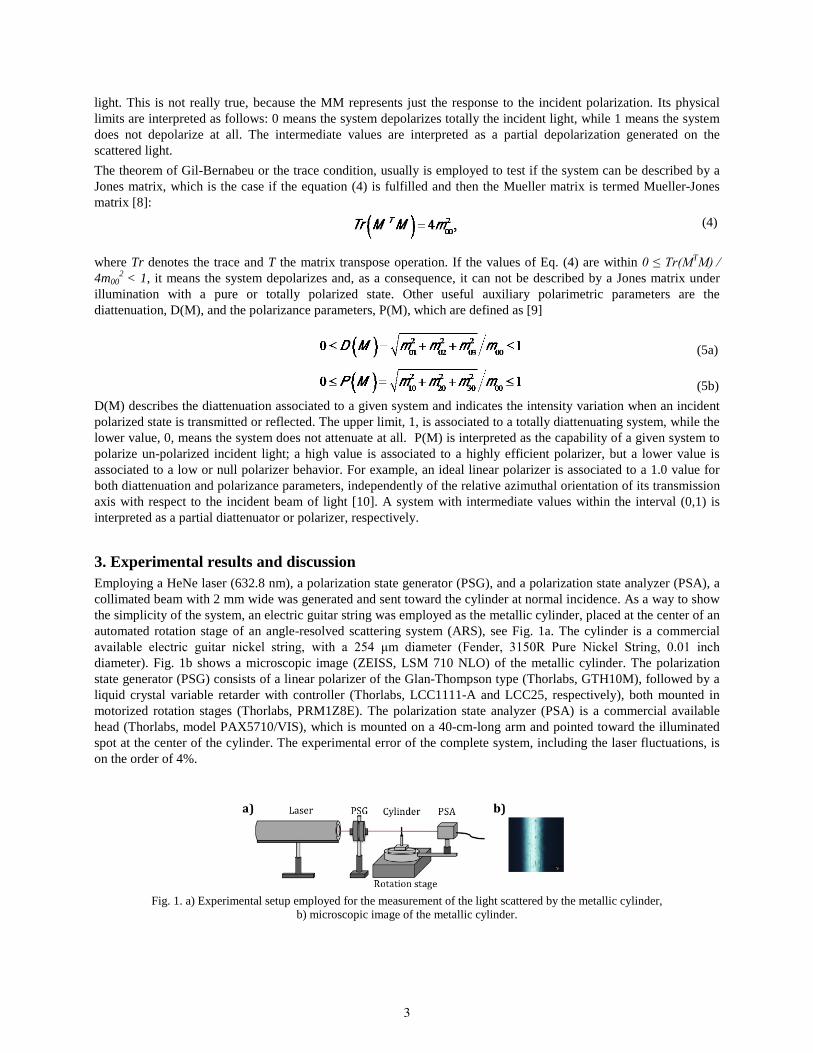
3. Experimental results and discussion Employing a HeNe laser (632.8 nm), a polarization state generator (PSG), and a polarization state analyzer (PSA), a collimated beam with 2 mm wide was generated and sent toward the cylinder at normal incidence. As a way to show the simplicity of the system, an electric guitar string was employed as the metallic cylinder, placed at the center of an automated rotation stage of an angle-resolved scattering system (ARS), see Fig. 1a. The cylinder is a commercial available electric guitar nickel string, with a 254 μm diameter (Fender, 3150R Pure Nickel String, 0.01 inch diameter). Fig. 1b shows a microscopic image (ZEISS, LSM 710 NLO) of the metallic cylinder. The polarization state generator (PSG) consists of a linear polarizer of the Glan-Thompson type (Thorlabs, GTH10M), followed by a liquid crystal variable retarder with controller (Thorlabs, LCC1111-A and LCC25, respectively), both mounted in motorized rotation stages (Thorlabs, PRM1Z8E). The polarization state analyzer (PSA) is a commercial available head (Thorlabs, model PAX5710/VIS), which is mounted on a 40-cm-long arm and pointed toward the illuminated spot at the center of the cylinder. The experimental error of the complete system, including the laser fluctuations, is on the order of 4%.

Fig. 1. a) Experimental setup employed for the measurement of the light scattered by the metallic cylinder, b) microscopic image of the metallic cylinder.

3

The scattered light is distributed on a plane surface, perpendicular to the cylinder axis. To obtain the Mueller matrix, a set of six polarization states was employed (linear horizontal p, perpendicular s, to +45°, -45°, and right- and left-handed circular polarization states, respectively). In the absence of any polarization-sensitive effect in the optical medium placed between the PSG and the PSA, the experimental setup was verified in order that each state of polarization detected corresponds to the same state of polarization generated.

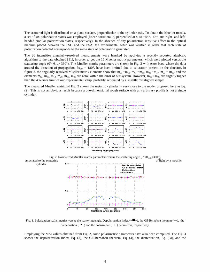
The 36 intensities angularly-resolved measurements were handled by applying a recently reported algebraic algorithm to the data obtained [11], in order to get the 16 Mueller matrix parameters, which were plotted versus the scattering angle (0°<θscatt<360°). The Mueller matrix parameters are shown in Fig. 2 with error bars, where the data around the direction of propagation, θscatt = 180°, have been omitted due to saturation present on the detector. In figure 2, the angularly-resolved Mueller matrix elements show that m00 ≅ m11, m01 ≅ m10, m22 ≅ m33, m23 ≅ -m32, and the elements m02, m03, m13, m20, m30, m31 are zero, within the error of our system. However, m12 ≅ m21 are slightly higher than the 4% error limit of our experimental setup, probably generated by a slightly misaligned sample.

The measured Mueller matrix of Fig. 2 shows the metallic cylinder is very close to the model proposed here as Eq. (2). This is not an obvious result because a one-dimensional rough surface with any arbitrary profile is not a single cylinder.

Fig. 2. Normalized Mueller matrix parameters versus the scattering angle (0°<θscatt<360°),

associated to the scattering of light by a metallic cylinder.

Fig. 3. Polarization scalar metrics versus the scattering angle. Depolarization index (−−), the Gil-Bernabeu theorem (−−), the diattenuation (−−) and the polarizance (−+−) parameters, respectively.

Employing the MM values obtained from Fig. 2, some polarimetric parameters have also been computed. The Fig. 3 shows the depolarization index, Eq. (3), the Gil-Bernabeu theorem, Eq. (4), the diattenuation, Eq. (5a), and the

4

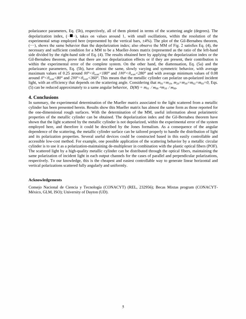
polarizance parameters, Eq. (5b), respectively, all of them plotted in terms of the scattering angle (degrees). The depolarization index, (−−), takes on values around 1, with small oscillations, within the resolution of the experimental setup employed here (represented by the vertical bars, ±4%). The plot of the Gil-Bernabeu theorem, (−−), shows the same behavior than the depolarization index; also observe the MM of Fig. 2 satisfies Eq. (4), the necessary and sufficient condition for a MM to be a Mueller-Jones matrix (represented as the ratio of the left-hand side divided by the right-hand side of Eq. (4). The results obtained here by applying the depolarization index or the Gil-Bernabeu theorem, prove that there are not depolarization effects or if they are present, their contribution is within the experimental error of the complete system. On the other hand, the diattenuation, Eq. (5a) and the polarizance parameters, Eq. (5b), have almost the same, slowly varying and symmetric behavior, with average maximum values of 0.25 around 80°<θscatt<180° and 180°<θscatt<280° and with average minimum values of 0.08 around 0°<θscatt<80° and 280°<θscatt<360°. This means that the metallic cylinder can polarize un-polarized incident light, with an efficiency that depends on the scattering angle. Considering that m01=m10, m20=m30=m02=m03=0, Eqs. (5) can be reduced approximately to a same angular behavior, D(M) = m01 ⁄ m00 ≅ m10 ⁄ m00. 4. Conclusions In summary, the experimental determination of the Mueller matrix associated to the light scattered from a metallic cylinder has been presented herein. Results show this Mueller matrix has almost the same form as those reported for the one-dimensional rough surfaces. With the determination of the MM, useful information about polarimetric properties of the metallic cylinder can be obtained. The depolarization index and the Gil-Bernabeu theorem have shown that the light scattered by the metallic cylinder is not depolarized, within the experimental error of the system employed here, and therefore it could be described by the Jones formalism. As a consequence of the angular dependence of the scattering, the metallic cylinder surface can be tailored properly to handle the distribution of light and its polarization properties. Several useful devices could be constructed based in this easily controllable and accessible low-cost method. For example, one possible application of the scattering behavior by a metallic circular cylinder is to use it as a polarization-maintaining de-multiplexer in combination with the plastic optical fibers (POF). The scattered light by a high-quality metallic cylinder can be distributed through the optical fibers, maintaining the same polarization of incident light in each output channels for the cases of parallel and perpendicular polarizations, respectively. To our knowledge, this is the cheapest and easiest controllable way to generate linear horizontal and vertical polarizations scattered fully angularly and uniformly.

Acknowledgements

Consejo Nacional de Ciencia y Tecnología (CONACYT) (REL, 232956); Becas Mixtas program (CONACYT-México, GLM, ISO); University of Dayton (UD).

5

Automatic calibration of 3D vision system via genetic algorithms and laser

line projection

Francisco Carlos Mejía Alanís and J. Apolinar Muñoz Rodríguez

Centro de Investigaciones en Optica A.C. f_mejia@cio.mx

munoza@foton.cio.mx ABSTRACT:

We present an automatic calibration via genetic algorithms and laser line imaging. This technique determines the vision parameters through genetic algorithms (GA) based on simulated binary crossover. To carry it out, an objective function is created from the laser line projection. Thus, the GA minimizes the objective function to determine the vision parameters. The proposed self-calibration improves the accuracy and performance of the three-dimensional vision system. It is because the errors in the physical measurements are not passed to the vision system. The advancement of our method is elucidated based on the accuracy of the self-calibration via GA. The results of self-calibration methods via least squared and gradient descent corroborate the contribution of the proposed self-calibration via the GA with SBX. Key words: Line projection, calibration, topography REFERENCES AND LINKS [1] N. Khaled, E. E. Hemayed, and M. B. Fayek, “A GA-based approach for epipolar geometry estimation”, International Journal of Pattern Recognition and Artificial Intelligence, Vol. 27, No. 8, p. 1355014-1-1355014-19, (2013). [2] A. Whitehead and G. Roth, “Estimating intrinsic camera parameters from the fundamental matrix using an evolutionary ppproach”, Journal on Applied Signal Processing, Vol.8, p. 1113–1124, (2004). [3] Z. Janko, D. Chetverikov and A. Ekart, “Using genetic algorithms in computer Vision: Registering images to 3D surface model”, Acta Cybernetica, Vol. 18, p.193–212, (2007). [4] Z. Talai, Y. M. Ben Ali, “Bio-Inspired solution for the homography problem”, Mathematical method in pattern recognition”, Vol.24, Vo.4, p.478-488, (2013). [5] C. H. Kao and R. C. Lo, “Camera self-calibration with planar pattern using genetic algorithms”, Applied Mechanics and Materials, Vol. 130, p.1833-1838, (2012). [6] N. Baran Hui and D. Kumar Pratihar, “Camera calibration using a genetic algorithm”, Engineering Optimization, Vol. 40, No. 12, p.151–1169, (2008). [7] B. Sareni, J. Regnier and X. Roboam, “Recombination and self-adaptation in multi-objective genetic algorithms”, Lecture notes in computer science, springer, vol. 2936, pp.115-126, (2004). [8] J. A. Muñoz Rodríguez and R. Rodríguez-Vera, “Evaluation of the light line displacement location for object shape detection”, Journal of Modern Optics, Vol. 50 No. 1 p. 137-154 (2003). [9] H. Frederick and G. J. Lieberman, Introduction to operations research, McGraw- Hill, USA, 1982. [10] K. Deep, M. Arya, M. Thakur and B. Raman, “Stereo camera calibration using particle swarm optimization”, Applied Artificial Intelligence, Vol. 27, p.618–634, (2013). [11] X. Wen-jiang, Z. Zhi-xiong, G. Dong-yuan, Z.Qing-ying and Y. Qing-he, “Camera Calibration by Hybrid Hopfield Network and Self-Adaptive Genetic Algorithm” Measurement science review, Vol. 12, No. 6, p. 302-308, (2012). [12] Q. Ji and Y. Zhang, “Camera Calibration with Genetic Algorithms”, IEEE Transactions on Systems, Man, and Cybernetics—Part A: Systems and Humans, VOL. 31, NO. 2, p. 120-130, (2001).

6

[13] P. Cerveri, A. Pedotti and N. A. Borghese, “Combined Evolution Strategies for Dynamic Calibration of Video-Based Measurement Systems”, IEEE Transactions on Evolutionary Computation, Vol. 5, NO. 3, p. 271-282, (2001). [14] G. G. Savii, “Camera calibration using compound genetic simplex algorithm”, Journal of Optoelectronics and Advanced Materials, Vol. 6, No. 4, p. 1255 – 1261, (2004). [15] S. Hati and S. Sengunpta, “Robust camera parameter estimation using genetic algorithms”, Pattern recognition letters, Vol.21, 289-298, (2001). [16] K. Zhang, B. Xu, L. Tang, H. Shi, “Modeling of binocular vision system for 3D reconstruction with improved genetic algorithms”, Int. J. Adv. Manuf. Technol., Vol. 29, p.722–728, (2006). 1. Introduction

Genetic algorithms (GAs) have improved the accuracy of the traditional calibration methods based on the gradient methods [1-2]. It is because GAs can find the global optimum in a high space avoiding be trapped in a local minima. Typically, the GA determines the vision parameters using an objective function, which is deduced from perspective projection, known references and image processing [3-4]. For instance, a GA achieves the calibration by means of an objective function, which is obtained by matching known points in a reference plane [5]. Another GA calibrates the vision parameters trough the objective function, which is defined by matching known points on the optical setup [6]. The aforementioned algorithms require external references to calibrate the vision parameters to perform 3-D vision. However, in several applications, the references are not supplied when the vision system is modified during the vision task. To solve this problem, it is necessary to implement a technique through GA without external references. The proposed calibration constructs an objective function from the setup geometry and image processing of the laser line position. Then, the simulated binary crossover (SBX) minimizes the objective function to obtain the vision parameters. Thus, the GA achieves the calibration and recalibration without external references. Also, the three-dimensional vision is carried out based on the laser line position. This proposed technique improves the accuracy and performance of the auto calibration via a GA and gradient methods. It is elucidated by an evaluation via traditional calibration methods based on GA with references. 2. Description self-calibration via genetic algorithm

The setup geometry for self-calibration is shown in Fig. 1(a), which includes an electromechanical device, a laser diode, a CCD camera, and a computer. The laser diode and the CCD are fixed perpendicularly to the surface. Also, the distance between the camera and the laser diode can be modified in x-axis. The x-axis and y-axis are located on the reference plane, which is perpendicular to z-axis. The focal length is indicated by f and the image center is indicated by (xc, yc). The distance between the optical axis and the laser line is indicated by L. The surface depth is indicated by hi,j and the distance from the lens to the reference plane is defined by D. The coordinates (xi,j, yi,j) indicate the laser line position on the image plane. Therefore, the projection of the laser line on the image plane is deduced from the setup geometry shown in Fig.1(a) and (b) by means of the next equations

)( ,

,ji

cji hD

LfX

x , (1)

)( ,

,ji

cji hD

BfY

y , (2)

)(

)(

,,

micmi hD

BCfY

y . (3)

In this case, Xi,m is computed via Eq.(1), where the i-index is replaced by the m-index. Thus, the objective function is defined via laser line position by means of the next equation

7

2,,2

,,2

,,2

,, mimijijimimijiji YYXXF yyxx , (4)

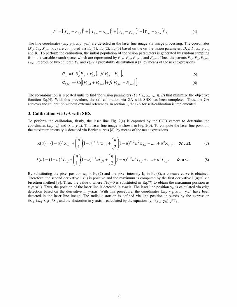
The line coordinates (xi,j, yi,j, xi,m, yi,m) are detected in the laser line image via image processing. The coordinates (Xi,j, Yi,j, Xi,m, Yi,m) are computed via Eq.(1), Eq.(2), Eq.(3) based on the on the vision parameters D, f, L, xc, yc, and B. To perform the calibration, the initial population of the vision parameters is generated by random sampling from the variable search space, which are represented by P1,i, P2,i, P1,i+1 , and P2,i+1. Thus, the parents P1,i, P2,i P1,i+1, P2,i+1, reproduce two children C1,i and C2,i via probability distribution β [7] by means of the next expressions

                                    iiiii PPPP ,1,2,2,1,1 5.0 C ,           (5)

                                    1,11,21,21,11,2 5.0 iiiii PPPP C , (6)

The recombination is repeated until to find the vision parameters (D, f, L, xc, yc, , B) that minimize the objective function Eq.(4). With this procedure, the self-calibration via GA with SBX has been completed. Thus, the GA achieves the calibration without external references. In section 3, the GA for self-calibration is implemented. 3. Calibration via GA with SBX

To perform the calibration, firstly, the laser line Fig. 2(a) is captured by the CCD camera to determine the coordinates (xi,j, yi,j) and (xi,m, yi,m). This laser line image is shown in Fig. 2(b). To compute the laser line position, the maximum intensity is detected via Bezier curves [8], by means of the next expressions

          jn

nj

nj

nj

n uuun

uun

uu ,,222

,11

,0 .....)1(2

)1(1

)1()( xxxxx

,      0≤ u ≤1.               (7)

jnn

jn

jn

jn IuIuu

nuIu

nIuuI ,,2

221,

1,0 .....)1(

2)1(

1)1()(

.         0≤ u ≤1.                 (8)

By substituting the pixel position xi,j in Eq.(7) and the pixel intensity Ii,j in Eq.(8), a concave curve is obtained. Therefore, the second derivative I”(u) is positive and the maximum is computed by the first derivative I’(u)=0 via bisection method [9]. Then, the value u where I´(u)=0 is substituted in Eq.(7) to obtain the maximum position as xi,j= x(u). Thus, the position of the laser line is detected in x-axis. The laser line position yi,j is calculated via edge detection based on the derivative in y-axis. With this procedure, the coordinates (xi,j, yi,j, xi,m, yi,m) have been detected in the laser line image. The radial distortion is defined via line position in x-axis by the expression xi,j=(x0,j–xi,j)-i*S1,j and the distortion in y-axis is calculated by the equation yj =(yi,0–yi,j)- j*Ti,1.

8

y-axis

Lens

L

f

h

hi,m

i,0

y y yi m,i,j c

D

x-axis

Optical axis

Lens

Laser line

L

f

h

hi,j

0,j

x xx0,ji,j c

D

Object

Object

Optical axis Laser line

hi,j

B

C

x yi j,i m,yi j,

(a) (b)

Fig. 1. (a) Geometry of the frontal view of the laser line projection in x-axis. (b) Geometry of lateral view laser line projection in

y-axis is described.

xi j, ,yi j,

xi,m,yi m, (a) (b)

Fig. 2 (a) Optical setup to perform self-calibration of vision parameters via GA. (b) Laser line image to detect reference coordinates.

Now, the GA is implemented based on the laser line position. To carry it out, the initial population is generated from the minimum and maximum value of each chromosome. Thus, the first parents P1,i,= P1,1, P2,i =P2,1, P1,i+1=P1,1+1 and P2,i+1,=P2,1+1 are stored in an array memory. Then, the parents create the first children C1,i =C1,1 and C2,i=C2,1 via SBX operator Eq. (5) and Eq. (6). Then, the fitness of each parent is computed via Eq. (4) for each parent. With this procedure, the population of the first generation has been completed. The second generation is constructed by means of the children and the best parents of the first generation. This procedure is carried out based on the best fitness. Thus, the parents of the second generation are defined by P1,2=P1,1,

9

P2,2= C1,1, P1,2+1= C2,1 and P2,2+1= P2,1+1. Then, the children of the second generation are created by substituting the parents P1,2, P2,2, P1,2+1 and P2,2+1 in Eq. (5) and Eq. (6). Thus, the children C1,2 and C2,2 are generated. Again, the objective function of each parent is computed via Eq. (4) to select the parents for the next generation. The procedure that creates the second generation is repeated until to find the parents that minimize the objective function Eq. (4). The chromosomes of these parents represent the vision parameters of the optical setup. Thus, the GA achieves the initial calibration to perform three-dimensional vision. The calibration accuracy and three-dimensional vision are described in section 4. 4. Experimental results of 3D scanner via auto-calibration

The object surface is scanned by laser line in x-axis and a set of images of laser line are captured by the CCD camera. From each image, the laser line position xi,j is calculated in each row by means of Eq.(7) and Eq.(8). Then, the object surface is computed by substituting the line position and the vision parameters in the expresion

,

,( )i jc i j

f Lh D

x x (9)

Thus, the whole object surface is reconstructed from the line position xi,j of all images. The test of the self-calibration via GA is performed for the reconstruction of a foot sole plaster shown in Fig. 3(a). The object coordinate xi,j corresponds to the position where the laser line is projected in x-axis. This coordinate is provided by the electromechanical slider. The object coordinate in y-axis is determined by substituting the line coordinate yi,j in the next expression

, , ,( ) ( )i j i j c i j cy D h y y y (10)

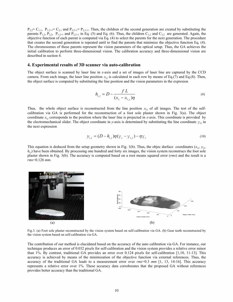
This equation is deduced from the setup geometry shown in Fig. 1(b). Thus, the objec durface coordinates (xi,j, yi,j, hi,j) have been obtained. By processing one hundred and forty six images, the vision system reconstrucs the foot sole plaster shown in Fig. 3(b). The accuracy is computed based on a root means squared error (rms) and the result is a rms=0.126 mm.

(a) (b) Fig.3. (a) Foot sole plaster reconstructed by the vision system based on self-calibration via GA. (b) Gear teeth reconstructed by the vision system based on self-calibration via GA.

The contribution of our method is elucidated based on the accuracy of the auto calibration via GA. For instance, our technique produces an error of 0.032 pixels for self-calibration and the vision system provides a relative error minor than 1%. By contrast, traditional GA provides an error over 0.124 pixels for self-calibration [1,10, 11-13]. This accuracy is achieved by means of the minimization of the objective function via external references. Thus, the accuracy of the traditional GA leads to a measurement error over rms=0.3 mm [1, 13, 14-16]. This accuracy represents a relative error over 1%. These accuracy data corroborates that the proposed GA without references provides better accuracy than the traditional GA.

10

Additionally, our GA is evaluated with respect to the self-calibration based on gradient and least squares method. For instance, it is reported that gradient methods produces a self-calibration error over 0.135 pixels and the error rms produced by the vision system is over 0.563 mm. Moreover, the least-squares method produces a self-calibration error over 0.1426 pixels and the error rms produced by the vision system is over 0.563 mm. The results of self-calibration methods via least squared and gradient descent corroborate the contribution of the proposed self-calibration via the GA with SBX. 5. Conclusions In the proposed vision system is allowed to reconfigure the setup during the vision task via GA re-calibration. Thus, flexible range measurements are achieved and occlusions are avoided. This technique improves the accuracy of traditional GA because it avoids measurements of external references. Also, our method improves the accuracy of the calibration via gradient methods. Therefore, this technique is performed in good manner.

11

Temperature measurement using a monochromatic schlieren system to analyze

combustion processes

José Antonio Cisneros Martínez (1), Cornelio Alvarez Herrera (2), Armando Gómez Vieyra (1)

1. División de Ciencias Básicas e Ingeniería, Universidad Autónoma Metropolitana, Unidad Azcapozalco. Av. San Pablo 180, C.P. 02200, México, D. F., México

2. Facultad de Ingeniería, Universidad Autónoma de Chihuahua. Circuito 1, Campus Universitario 2, C.P. 31125, Chihuahua, Chih., México.

Corresponding author email: crwxss1@gmail.com

ABSTRACT:

This work is based on the use of the Schlieren optical system using light source in different wavelengths. The wavelengths used were obtained from LEDs in colors such as yellow, blue, white, purple, orange, red, pink and green, which were characterized for their spectral bands. As test object, a butane flame was used. From the hot gases caused by the flame, intensity gradients in 2D were obtained in gray scale, for each wavelength. Temperature fields 2D were obtained qualitatively from intensity gradients, showed in normalized form due to the Schlieren system is not calibrated at this point of the research. Our interest was to explore the process of chemical absorption using light sources with spectral bands limited such as LEDs to get a better understanding of the combustion in the flame. Schlieren technique applied with different wavelengths reveals more details about the combustion in flames as predicted the Gladstone-Dale relation.

Key words: Schlieren, temperature, flames, LEDs

REFERENCES AND LINKS [1] R. M. Fristrom, “Flame Sampling for mass spectrometry”, Int, J. Mass Spectrom. Ion Phys. 16, 15-32 (1975). [2] Knuth, Engine Emissions: Pollutant Formation and Measurement, Springer and Patterson, (1973). [3] A. C. Eckbreth, “Recent advances in laser diagnostics for temperature and species concentrations in combustion”, Symp. Combust. 18, 1471-1488 (1981). [4] R. K. Miller, B. and Hansen, “Homogeneus: LDV Using Iodine Seeding”, Appl. Phys. Lett. 43, (1983). [5] V. CM., Holographic Interferometry Wiley, (1979). [6] F. NA. Speckle Photography for Fluid Mechanics Measurements, Springer, (1998). [7] G. S. Settless, Schlieren and Shadowgraph Techniques, first ed. Springer, Berlin, (2001). [8] W. Merzkirch, Flow Visualization, Second ed. Academic Press, Orlando (1987). [9] C. Alvarez-Herrera, D. Moreno-Hernández, and B, Barrientos-García, “Temperature measurement of an axisymmetric flame by using a schlieren system” J. Opt. A Pure Appl. 10, 104014 (2008). [10] A. G. Gaydon and H. G. Wolfhard, Radiation Processes in Flames, Their structure, Radiation and Temperature, Third Edit, Chapman and Hall, pp. 211-215 (1987). [11] A. G. Gaydon and H. G. Wolfhard, “Spectroscopic studies of low-Presure flames”, Symp. Combust. Flame, Explos. Phenom. 3, 504-518 (1948).

12

1. Introduction It is known that any heat source in contact with a fluid, will transfers heat to the fluid, appearing a temperature gradient and a density gradient too. In consequence a refractive gradient index will appear if the fluid heated by the heat source is a transparent medium. The differences between the refractive index in the transparent medium deviates a light ray that pass through of it, acting it as an optical lens. Using our eyes as sensors we cannot observe these differences between the refractive index so a wide variety of optical instruments to visualize these differences are used.

A variety of techniques to study the combustion process are used. To specification of the combustion requires measurement of variables such as temperature gas speed and profiles of composition as a distance function through the front flame. The experimental methods have been realized to study these subjects [1],[2],[3], between the most important are physical tests and optical tests. Physical tests perturb the flame and optical tests not, by these reasons optical tests in this work are used.

Optical tests of full field are those that allow to determine temperature in a transparent medium or in this case transparent fluid, in a zone delimited by the vision field of the optical instruments used in the test. Optical methods represent nonintrusive tools to visualize the fluid in movement and the temperature distribution on real time at full field. The different optical tests available allow us to measure all the properties of interest in combustion. A complete analysis requires several complemented techniques to accommodate the long rate of concentrations and kind of species found in combustion. Some optical methods are LDV (Laser Doppler Velocimetry) [4], Holographic Interferometry [5], Laser Speckle [6] and Schlieren [7].

Schlieren technique is common used to visualize and measure temperature and other gas properties. The interest in this technique to measure temperature is due to their easy implementation, low cost, uses conventional light sources and is sensible to the refractive changes of the transparent medium.

2. Theoretical Background 2.a. Light Propagation in Inhomogeneous Media

Light propagates uniformly through a homogeneous medium. Light travels lent when interacts with mater. The refractive index n = c0/c, where c=3x108 m/s, is the light speed in vacuum and c0 is the light speed in the medium. To air and other gases there is a simple linear relation between refractive index and gas density ρ.

Kn 1 , (1)

K is the Gladstone-Dale constant and depends of the wavelength used as a light source and of the substance used as a transparent media, for the air K=0.23 cm3/g at normal conditions. For other gases the constant vary between 0.1 to 1,5 cm3 /g. In Eq. (1) n depends of ρ. For most of the cases temperature, density and pressure are related by state equation of ideal gas

RTP . (2)

Where R is the specific gas constant. The gases with variable density are called compressible fluids; that can be caused by the temperature or high speed gas variation. All these possibilities conduct to gas perturbations that refract the light and can be visualized thanks to this phenomenon.

The refractivity (n-1) has some characteristics that are used [8]. For example, when K slightly diminishes the wave length λ grows. Thus the refractivity grows for small λ, the most weak disturbs are more detectable with ultraviolet light than visible light.

Our interest is the deviation of light ray when pass through an inhomogeneous medium. Using the Cartesian system at right side of Fig. 1, the z-axis will be the direction of light ray propagation.

13

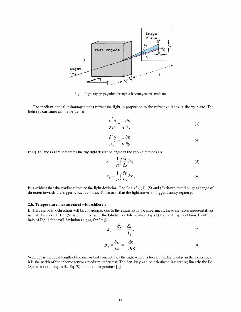
Fig. 1. Light ray propagation through a inhomogeneous medium.

The medium optical in-homogeneities refract the light in proportion to the refractive index in the xy plane. The light ray curvature can be written as

x

n

nz

x

12

2

, (3)

y

n

nz

y

12

2

, (4)

If Eq. (3) and (4) are integrates the ray light deviation angle in the (x,y) directions are

zx

n

nx

1 , (5)

zy

n

ny

1 , (6)

It is evident that the gradients induce the light deviation. The Eqs. (3), (4), (5) and (6) shows that the light change of direction towards the bigger refractive index. This means that the light moves to bigger density region ρ.

2.b. Temperature measurement with schlieren

In this case only x-direction will be considering due to the gradients in the experiment, these are more representatives in that direction. If Eq. (5) is combined with the Gladstone-Dale relation Eq. (1) the next Eq. is obtained with the help of Fig. 1 for small deviation angles, for l = f2.

2f

x

l

xx

, (7)

hKf

x

xx2

(8)

Where f2 is the focal length of the mirror that concentrates the light where is located the knife edge in the experiment, h is the width of the inhomogeneous medium under test. The density ρ can be calculated integrating linearly the Eq. (8) and substituting in the Eq. (9) to obtain temperature [9].

14

00

00

1

1T

n

nTT

(9)

Where n0 and ρ0 are the refractive index and density at reference temperature T0 and T is the temperature measured.

2.c. Spectroscopy in the combustion processes

The continuum spectrums are emitted by the hot solid bodies but in some cases, the continued emission regions can be due to process such as the ion combinations or association of atoms or radicals. For molecules in gaseous state, the energy of each molecule is restrained to a limited number of possible values, in other word is quantified and the radiation wave lengths that the molecules can emit or absorb are limited to a number relatively small of spectral lines. The spectrum in visible and in ultraviolet regions are generally due to the changes of electronic energy, in other words, a transition of electron configurations over the molecule to other configuration. This change determines the position of the band systems as a whole. The changes that accompany vibration energy of the molecular atoms, determine the position of the individual bands inside the band systems. The changes that accompany the rotation energy of the molecule determine the fine structure of the individual bands, furthermore, the structure of the fine band line. The band spectrums in near infrared are due to changes of vibrational and rotational energy of the molecules, while the spectrums in the far infrared are due to the rotation energy changes only. In Bunsen flames, much unstable radicals can be formed such as CH, C2, HCO, NH, NH2, etc., these give an appreciable emission in the visible and the near ultraviolet.

The H2O has strong vibration bands in 1.8, 2.7 and 6.3µ and a rotation band that covers the region of 10-100µ. The CO2 emits in 2.8, 4.3 and 15µ. Other vibrational bands of interest are the CO in 2.3 and 4.5 µ, el NO in 2.6 and 5.2 µ and the vibrational bands of OH cover the near infrared area around 4 µ. This follows the Wien displacement law (λmT=0.289[cm K]), this means that maximum flame temperatures tend to be in the near infrared between 2 and 1 µ approximately according to the flame temperature as shown in Fig. 2. To clear flames the radiation in the visible and ultraviolet are less than 0.4% of the produced heat by the combustion. This visible radiation cams from internal cone mainly, while the infrared radiation cams from the main body of the gases, of both parts internal cone and burned products. To luminous flames, the radiation of heated carbon particles, increase the radiation in the visible. For more heated flames with the oxygen, we expect an increase of radiation. Further information can be seen in [10],[11].

Fig.2. Black body radiation at different temperatures as function of wave length [10].

3. Experiment In this section the experiment used for this research will be described briefly. To obtain the temperature gradients produced by a butane air flame the characterization of the light source was made. Then each LED was characterized

15

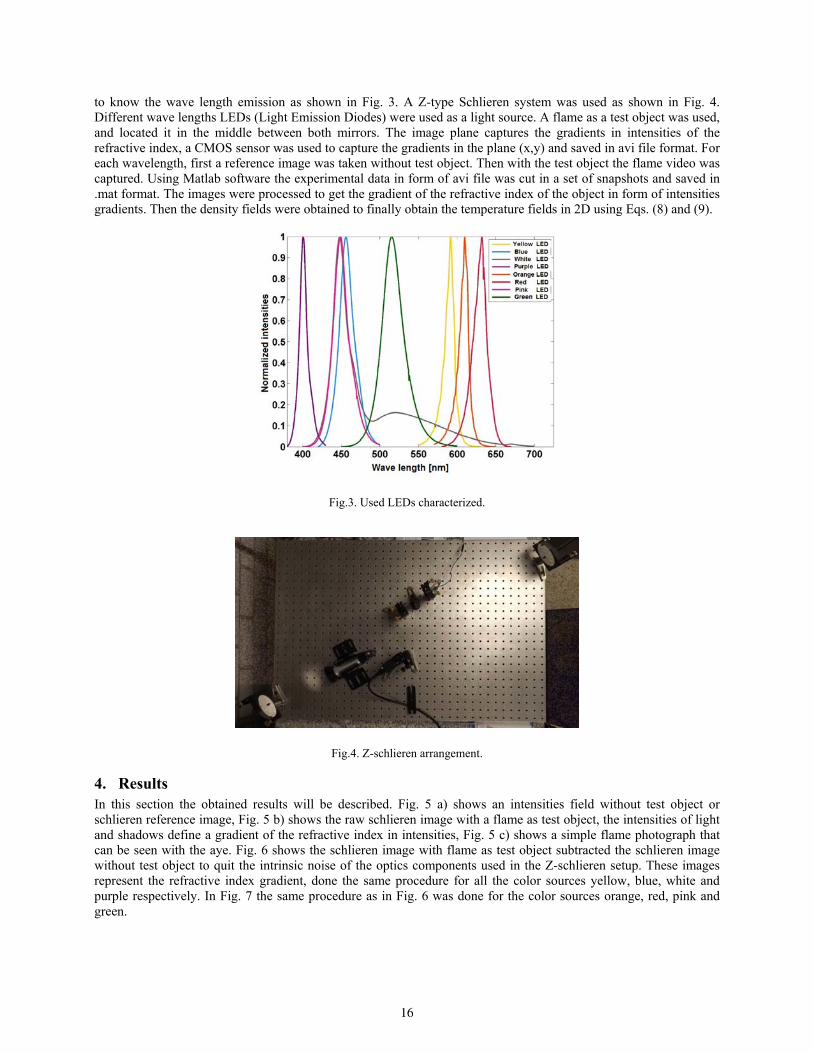
to know the wave length emission as shown in Fig. 3. A Z-type Schlieren system was used as shown in Fig. 4. Different wave lengths LEDs (Light Emission Diodes) were used as a light source. A flame as a test object was used, and located it in the middle between both mirrors. The image plane captures the gradients in intensities of the refractive index, a CMOS sensor was used to capture the gradients in the plane (x,y) and saved in avi file format. For each wavelength, first a reference image was taken without test object. Then with the test object the flame video was captured. Using Matlab software the experimental data in form of avi file was cut in a set of snapshots and saved in .mat format. The images were processed to get the gradient of the refractive index of the object in form of intensities gradients. Then the density fields were obtained to finally obtain the temperature fields in 2D using Eqs. (8) and (9).

Fig.3. Used LEDs characterized.

Fig.4. Z-schlieren arrangement.

4. Results In this section the obtained results will be described. Fig. 5 a) shows an intensities field without test object or schlieren reference image, Fig. 5 b) shows the raw schlieren image with a flame as test object, the intensities of light and shadows define a gradient of the refractive index in intensities, Fig. 5 c) shows a simple flame photograph that can be seen with the aye. Fig. 6 shows the schlieren image with flame as test object subtracted the schlieren image without test object to quit the intrinsic noise of the optics components used in the Z-schlieren setup. These images represent the refractive index gradient, done the same procedure for all the color sources yellow, blue, white and purple respectively. In Fig. 7 the same procedure as in Fig. 6 was done for the color sources orange, red, pink and green.

16

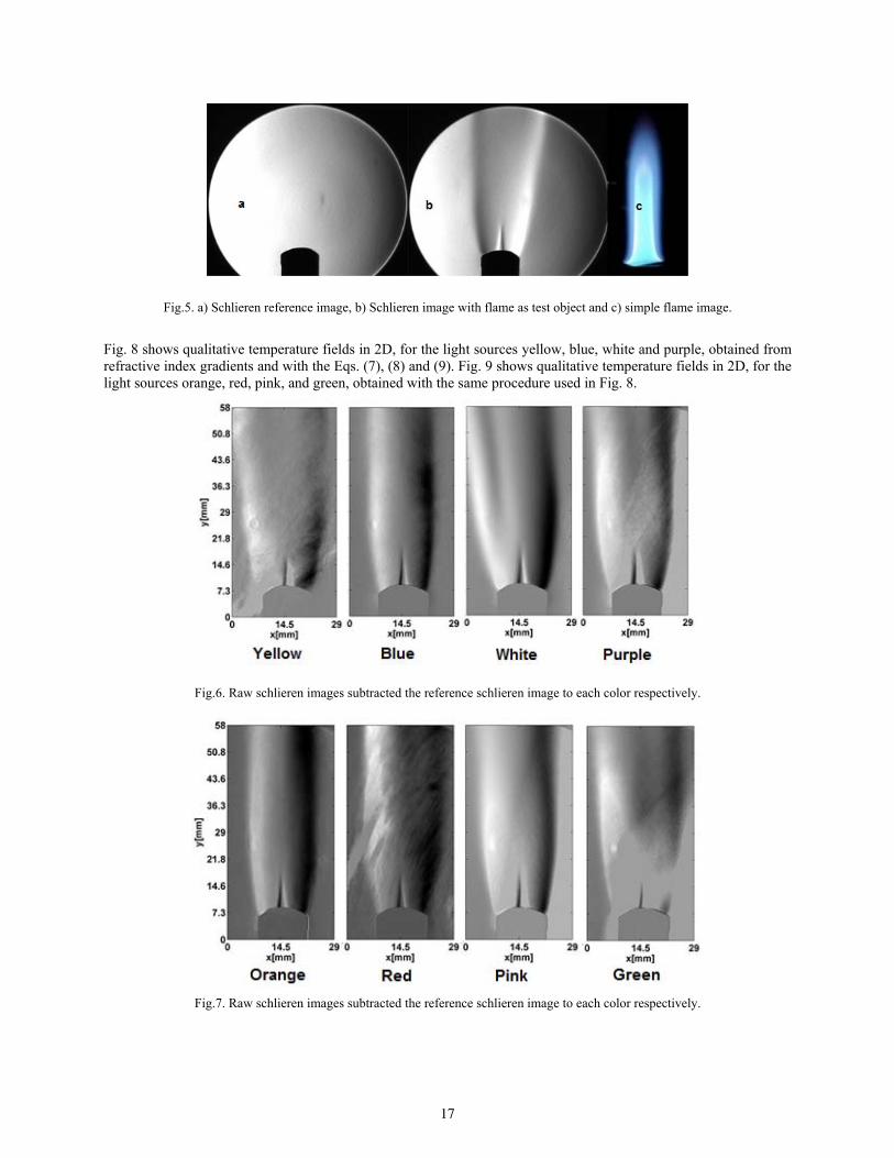
Fig.5. a) Schlieren reference image, b) Schlieren image with flame as test object and c) simple flame image.

Fig. 8 shows qualitative temperature fields in 2D, for the light sources yellow, blue, white and purple, obtained from refractive index gradients and with the Eqs. (7), (8) and (9). Fig. 9 shows qualitative temperature fields in 2D, for the light sources orange, red, pink, and green, obtained with the same procedure used in Fig. 8.

Fig.6. Raw schlieren images subtracted the reference schlieren image to each color respectively.

Fig.7. Raw schlieren images subtracted the reference schlieren image to each color respectively.

17

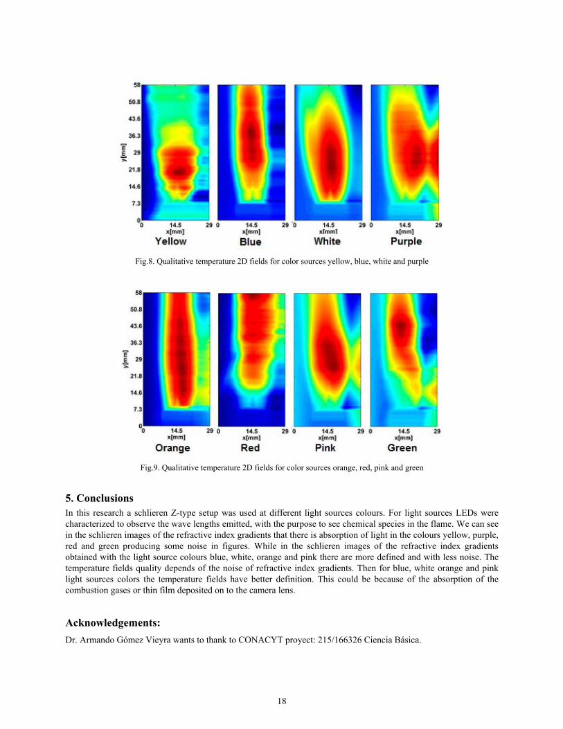
Fig.8. Qualitative temperature 2D fields for color sources yellow, blue, white and purple

Fig.9. Qualitative temperature 2D fields for color sources orange, red, pink and green

5. Conclusions In this research a schlieren Z-type setup was used at different light sources colours. For light sources LEDs were characterized to observe the wave lengths emitted, with the purpose to see chemical species in the flame. We can see in the schlieren images of the refractive index gradients that there is absorption of light in the colours yellow, purple, red and green producing some noise in figures. While in the schlieren images of the refractive index gradients obtained with the light source colours blue, white, orange and pink there are more defined and with less noise. The temperature fields quality depends of the noise of refractive index gradients. Then for blue, white orange and pink light sources colors the temperature fields have better definition. This could be because of the absorption of the combustion gases or thin film deposited on to the camera lens.

Acknowledgements:

Dr. Armando Gómez Vieyra wants to thank to CONACYT proyect: 215/166326 Ciencia Básica.

18

A digital image pattern recognition system invariant to rotation, scale and translation for color images

Carolina Barajas-García (1), Selene Solorza-Calderón (1), Josué Álvarez-Borrego (2)

1. Facultad de Ciencias, Universidad Autónoma de Baja California, México.

2. Div. de Física Aplicada, Centro de Investigación Científica y de Educación Superior de Ensenada, México. Corresponding author email: selene.solorza@gmail.com

ABSTRACT:

This work presents a new pattern recognition system for color images invariant to rotation, scale and translation (RST). The digital system is based on the Fourier transform, the normalized analytic Fourier-Mellin transform and Bessel binary rings masks to generate 1D RST invariant signatures for each channel in the RGB color space. Using the instantaneous amplitudes of those 1D signatures a classifier cuboids space with confidence level of 95.4% is constructed.

Key words: Pattern recognition, feature extraction, color image, 1D signature, Bessel masks.

REFERENCES AND LINKS

[1] B.L. Boese, P.J. Clinton, D. Dennis, R.C. Golden y B. Kim, “Digital image analysis of Zostera marina leaf injury”, Aquat. Bot. 88, 87-90 (2008).

[2] D.G. Lowe, “Distinctive image features from scale-invariant key points”, IJCV 60, 91-110 (2004).

[3] H. Bay, A. Essa, T. Tuytelaars y L. Van Gool, “Speeded-Up Robust Features (SURF)”, CVIU 110, 346-359 (2008).

[4] Y. Ke y R. Sukthankar, “PCA-SIFT: A more distinctive representation for local image descriptors”, CVPR, 506-513 (2004).

[5] E.N. Mortensen, H. Deng y L. Shapiro, “A SIFT descriptor with global context”, CVPR 1, 184-190 (2005).

[6] D. Su, J. Wu, Z. Cui, V.S. Sheng y S. Gong, “CGCI-SIFT: A more efficient and compact representation of local descriptor” Meas. Sci. Rev. 13, 132-141 (2013).

[7] A.E. Abdel-Hakin y A.A. Farag, “CSIFT: A SIFT descriptor with color invariant characteristics”, CVPR, 1978-1983 (2006).

[8] R. Javanmard-Alitappeh, K. Jeddi-Saravi y F. Mahmoudi, “A new illumination invariant feature based on SIFT descriptor in color space”, Procedia Eng. 41, 305-311 (2012).

[9] C. Ancuti y P. Bekaert, “SIFT-CCH: Increasing the SIFT distinctness by color co-occurrence histograms”, ISPA, 130-135 (2007).

[10] S. Solorza y J. Álvarez-Borrego, “Translation and rotation invariant pattern recognition by binary rings masks”, J. Mod. Opt. 62, 851-864 (2015).

[11] S. Derrode y F. Ghorbel, “Robust and efficient Fourier-Mellin transform approximations for Gray-level image reconstruction and complete invariant description”, CVIU 83, 57-78 (2001).

19

1. Introduction

Reproduce the pattern recognition human functions are a great challenge and a very difficult task. The research community has been employed a lot effort to create robots and automation systems to this purpose. Color is a very important feature to human pattern recognition process, if this information is neglected very important characteristic could be lost. For example, the color is used to study the Zostera marina leaf injury [1], but the processing of the images is done by hand-operated through multiple imaging programs (Adobe PhotoShop, Canon Photostitch and ERMapper) although local feature descriptors are used in a variety of pattern recognition real-world applications due to the identification efficiency [2-5]. The color-SIFT descriptors are developed to take into account the color feature, but the complexity and the calculation increase considerably for the training and the testing phases [6-9].

This work presents a rotation, scale and translation (RST) invariant color image descriptor based on Bessel binary rings masks methodology developed in [10]. This RT invariant methodology is robust and efficient in the pattern recognition for gray-level images regardless the position and rotation the object presents. To introduce the scale invariance, here is proposed the use of the amplitude spectrum of the normalized analytic Fourier-Mellin transform (AFMT). This spectrum is filtered by a Bessel binary rings mask in order to obtain a RST invariant 1D signature for each channel in the RGB color space. The instantaneous amplitudes of the signatures for the training color images are used to construct cuboids with 95.4% confidence level (based on the statistical boxplot technique); those cuboids are used to build the classifier space; in this manner, the classification step reduces considerably the computational time investment. The rest of the work is organized as follows: Section 2 describes the procedure to develop the RST invariant color image pattern recognition system based on Bessel masks. Section 3 exposes the methodology to construct the classifier cuboids space. Finally, conclusions are given in section 4.

2. The RST Invariant Pattern Recognition System for Color Images

2.a. The Bessel binary rings masks

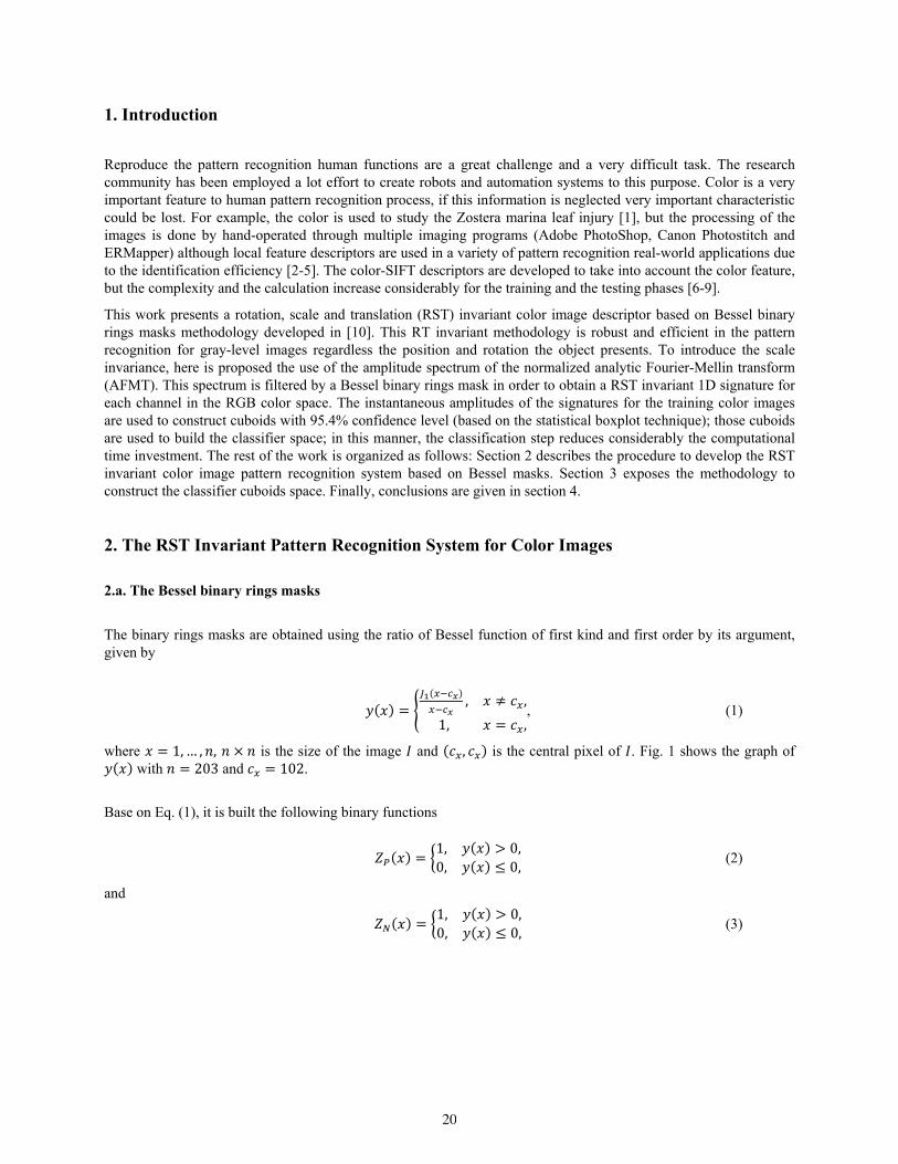
The binary rings masks are obtained using the ratio of Bessel function of first kind and first order by its argument, given by

, ,

1, ,, (1)

where 1,… , , is the size of the image and , is the central pixel of . Fig. 1 shows the graph of with 203 and 102.

Base on Eq. (1), it is built the following binary functions

1, 0,0, 0,

(2)

and

1, 0,0, 0,

(3)

20

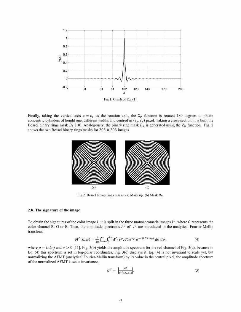
Fig.1. Graph of Eq. (1).

Finally, taking the vertical axis as the rotation axis, the function is rotated 180 degrees to obtain concentric cylinders of height one, different widths and centred in , pixel. Taking a cross-section, it is built the Bessel binary rings mask [10]. Analogously, the binary ring mask is generated using the function. Fig. 2 shows the two Bessel binary rings masks for 203 203 images.

Fig.2. Bessel binary rings masks. (a) Mask . (b) Mask .

2.b. The signature of the image

To obtain the signatures of the color image , it is split in the three monochromatic images , where represents the color channel R, G or B. Then, the amplitude spectrums of are introduced in the analytical Fourier-Mellin transform

, , , (4)

where and 0 [11]. Fig. 3(b) yields the amplitude spectrum for the red channel of Fig. 3(a), because in Eq. (4) this spectrum is set in log-polar coordinates, Fig. 3(c) displays it. Eq. (4) is not invariant to scale yet, but normalizing the AFMT (analytical Fourier-Mellin transform) by its value in the central pixel, the amplitude spectrum of the normalized AFMT is scale invariance,

,

. (5)

21

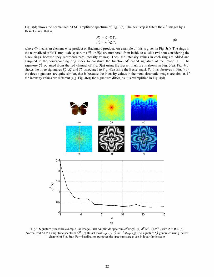
Fig. 3(d) shows the normalized AFMT amplitude spectrum of Fig. 3(c). The next step is filters the images by a Bessel mask, that is

⨂ ,⨂ ,

(6)

where ⊗ means an element-wise product or Hadamard product. An example of this is given in Fig. 3(f). The rings in the normalized AFMT amplitude spectrum ( or ) are numbered from inside to outside (without considering the black rings, because they represents zero-intensity values). Then, the intensity values in each ring are added and assigned to the corresponding ring index to construct the function called signature of the image [10]. The signature obtained from the red channel of Fig. 3(a) using the Bessel mask is shown in Fig. 3(g). Fig. 4(b) shows the three signatures , and associated to Fig. 4(a) using the Bessel mask . It is observes in Fig. 4(b), the three signatures are quite similar, that is because the intensity values in the monochromatic images are similar. If the intensity values are different (e.g. Fig. 4(c)) the signatures differ, as it is exemplified in Fig. 4(d).

Fig.3. Signature procedure example. (a) Image . (b) Amplitude spectrum , . (c) , , with 0.5. (d) Normalized AFMT amplitude spectrum . (e) Bessel mask . (f) ⨂ . (g) The signature generated using the red

channel of Fig. 3(a). For visualization purposes the spectrums are given in logarithmic scale.

22

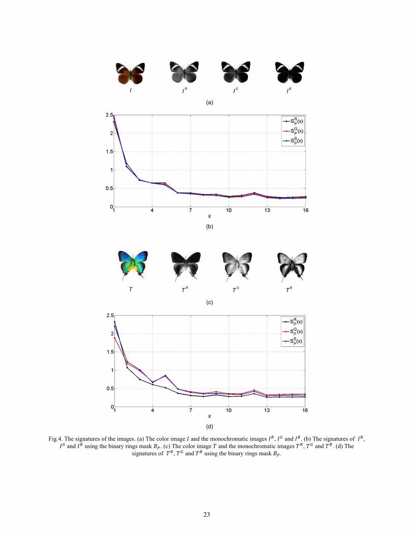
Fig.4. The signatures of the images. (a) The color image and the monochromatic images , and . (b) The signatures of , and using the binary rings mask . (c) The color image and the monochromatic images , and . (d) The

signatures of , and using the binary rings mask .

23

The features selected to characterize the image are the instantaneous amplitude of the signatures, given by

∑ , (7)

where or .

3. The classifier cuboids space

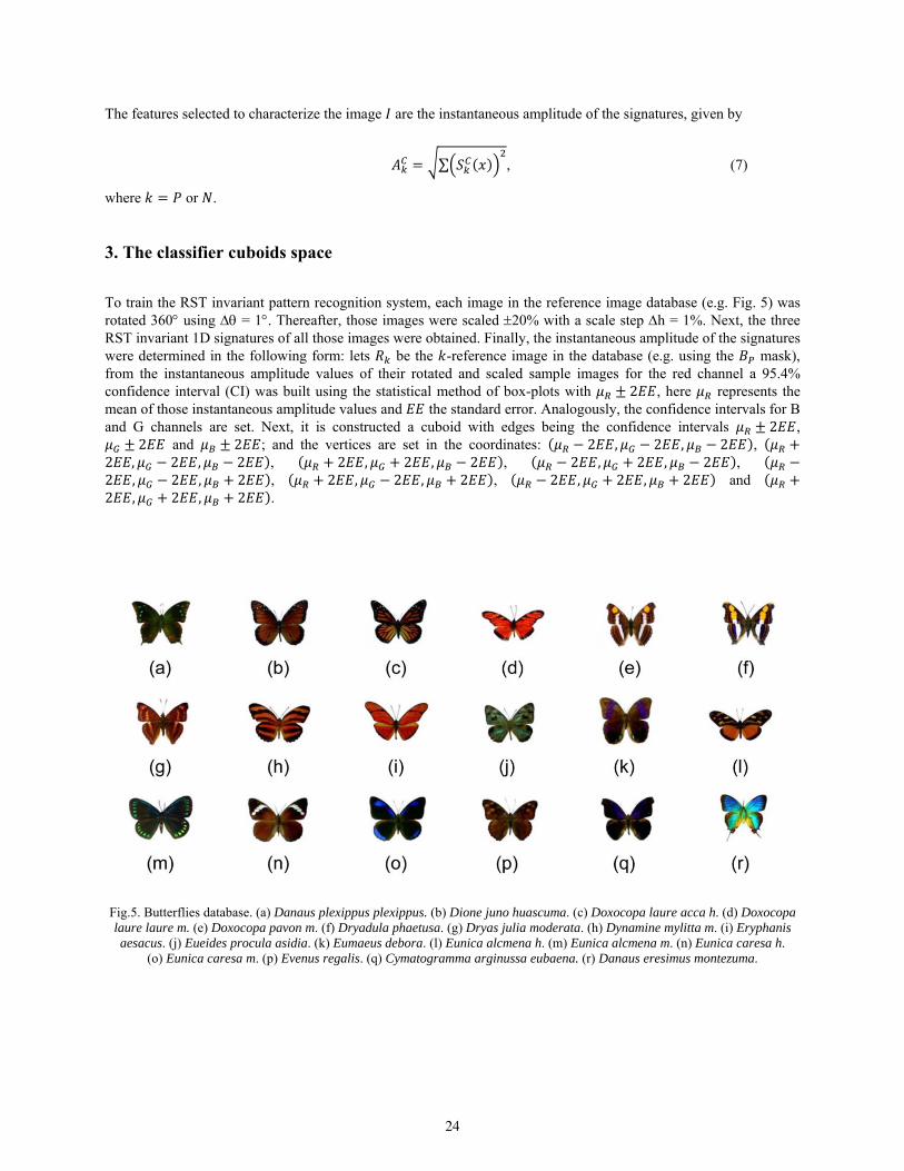
To train the RST invariant pattern recognition system, each image in the reference image database (e.g. Fig. 5) was rotated 360 using = 1. Thereafter, those images were scaled 20% with a scale step h = 1%. Next, the three RST invariant 1D signatures of all those images were obtained. Finally, the instantaneous amplitude of the signatures were determined in the following form: lets be the -reference image in the database (e.g. using the mask), from the instantaneous amplitude values of their rotated and scaled sample images for the red channel a 95.4% confidence interval (CI) was built using the statistical method of box-plots with 2 , here represents the mean of those instantaneous amplitude values and the standard error. Analogously, the confidence intervals for B and G channels are set. Next, it is constructed a cuboid with edges being the confidence intervals 2 ,

2 and 2 ; and the vertices are set in the coordinates: 2 , 2 , 2 , 2 , 2 , 2 , 2 , 2 , 2 , 2 , 2 , 2 , 2 , 2 , 2 , 2 , 2 , 2 , 2 , 2 , 2 and 2 , 2 , 2 .

Fig.5. Butterflies database. (a) Danaus plexippus plexippus. (b) Dione juno huascuma. (c) Doxocopa laure acca h. (d) Doxocopa laure laure m. (e) Doxocopa pavon m. (f) Dryadula phaetusa. (g) Dryas julia moderata. (h) Dynamine mylitta m. (i) Eryphanis aesacus. (j) Eueides procula asidia. (k) Eumaeus debora. (l) Eunica alcmena h. (m) Eunica alcmena m. (n) Eunica caresa h.

(o) Eunica caresa m. (p) Evenus regalis. (q) Cymatogramma arginussa eubaena. (r) Danaus eresimus montezuma.

24

Fig. 6 and Fig. 8 show the classifier cuboids space for the database in Fig. 5 using and masks, respectively. Hence, a volume space could be assigned to each image without overlapping (Fig. 7 shows an amplification zone of the output space to observe the cuboids assigned to some butterflies); in both cases, the RST invariant pattern recognition color image presents a confidence level at least of 95.4%. Contrary at correlator pattern recognition systems in [10] (where multiple correlation output planes are generated: one for each image in the database) here is established one classifier space, achieving in this form reduces the computational time investment.

Fig.6. Classifier cuboids space using the Bessel mask .

Fig.7. Amplification zone of the classifier cuboids space using the Bessel mask .

25

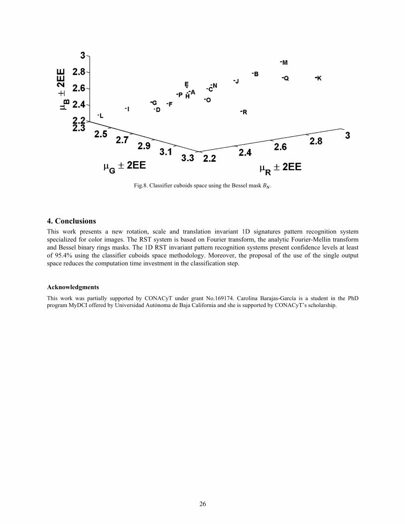
Fig.8. Classifier cuboids space using the Bessel mask .

4. Conclusions This work presents a new rotation, scale and translation invariant 1D signatures pattern recognition system specialized for color images. The RST system is based on Fourier transform, the analytic Fourier-Mellin transform and Bessel binary rings masks. The 1D RST invariant pattern recognition systems present confidence levels at least of 95.4% using the classifier cuboids space methodology. Moreover, the proposal of the use of the single output space reduces the computation time investment in the classification step.

Acknowledgments

This work was partially supported by CONACyT under grant No.169174. Carolina Barajas-García is a student in the PhD program MyDCI offered by Universidad Autónoma de Baja California and she is supported by CONACyT’s scholarship.

26

Optical Analysis of the Gecko Eye with an Elliptical to Circular Pupil Transformation

Francisco Javier Renero Carrillo, Gonzalo Urcid Serrano, Luis David Lara Rodríguez, and

Elizabeth López Meléndez

Optics Department, INAOE, Tonanzintla, Puebla, México. Corresponding author email: elom@inaoep.mx

ABSTRACT: Biologists have found that most animals with elliptical and rectangular pupils can distinguish more colors than those with circular pupils. As an example of this natural color achievement by the animal’s eye, here, we describe briefly the Gecko’s eye, as well as a simplified geometrical model to understand its basic night colored vision mechanism. The Gecko is a small terrestrial reptile that belongs to the Gekkonidae family. The specific characteristics of the Gecko’s eye are the following: the eyeball has an approximate diameter of 3.9 mm, compounded of three optical surfaces with different curvature radii and refraction indexes between them; its nocturnal vision ranges from ultraviolet to the visible spectrum. Additionally, the Gecko’s eye pupil changes form dynamically from a very elongated ellipse to practically a circle depending of the luminance received from a natural light source. Thereafter, we discuss mathematically the pupil transformation from an elliptical to a circular shape that is used in our optical analysis. First, we compute, for selected wavelength values belonging to the Gecko’s specific night vision spectral ranges, the spot diagrams and the corresponding modulation transfer functions in order to determine the Gecko’s spatial resolution. Then we compute the near and far field diffraction patterns in order to discuss the Gecko’s pupil diffraction dynamics. All the previous computations are given for a finite set of eccentricity values and at specific wavelengths and some of these results are presented graphically. Finally, we simulate the Gecko’s eye image formation for simple input objects under assumed low-level light conditions including pertinent comments about this particular multi-focal optical system.

Keywords: Gecko, Diffraction patterns, Circular pupil, Elliptical pupil, Wavelength

REFERENCES AND LINKS [1] Nocturnal helmeted Gecko image available from, www.moroccoherps.com

[2] Smith, W. J., Modern Optical Engineering: Design of optical systems, 4nd edition, McGraw Hill Education, New York, NY, 2007.

[3] Renero C., F.J., “Automatic Design of Lens Arrays for Optical Computing and Interconnects”, Applied physics, Osaka University, Japan, (1995).

[4] Goodman, J. W., Introduction to Fourier Optics, 3rd edition, Roberts & Co. Englewood, Colorado, 2005.

[5] Roth, L.S.V., Lundström, L., Kelber, A., Kröger, R.H.H., and Unsbo, P., “The pupils and optical systems of gecko eyes,” Journal of Vision, 9(3):27, 1 –11, 2009.

[6] Renero-C, F. J., Exploring fabrication tolerances of optical systems by solving inequalities. Optik-International Journal for Light and Electron Optics, 121 (24), 2280-2283, (2010).

[7] The Mathworks Inc., The Language of Scientific Computing, www.mathworks.com/product/matlab

[8] Roth, L.S.V., Kelber, A., “Nocturnal color vision in geckos,” The Royal Society Biological Letters, 271, S485-S487, 2004.

27

1. Introduction The nocturnal helmeted Gecko1 is a small terrestrial reptile that belongs to the Gekkonidae family, see Fig. 1. It lives at South of Morocco, Mauritania and west Sahara to Senegal. Their body size is about 6 to 9 cm and its nocturnal vision ranges from long wave ultraviolet to the visible spectrum. The Gecko’s eye ball has an approximate diameter of 3.9 mm and its pupil changes shape depending on light conditions; if more illumination gets into the pupil it will become almost a line, if less illumination the pupil of the Gecko will become a circle.

Fig. 1. Nocturnal helmeted Gecko.

2. Refraction Index and Diffraction Patterns Computation When aberrations exceed several times the Rayleigh resolution limit, diffraction effects are negligible and the result of ray tracing can predict the image of a point with a good degree of accuracy. This is done by dividing the entrance pupil of the optical system in a large number of equal areas for a ray trace of an object point through the center of each small area. The intersection of each ray on the image plane is plotted as each beam represents a similar contribution of the total energy in the image, then the density of the points is plotted as power density (irradiance, luminance) image. Light intercepted in such graphs is called spot diagram2; all the rays in this work have circular symmetry. A lens type commonly used to test the performance of a lens system consists of a series of brilliant and opaque bars of equal width. Various sets of patterns with different spacing are usually obtained from the system under test. If these line patterns can be distinguish, we can obtain the resolving power of the system, expressed by a number of line pair per millimeter (a line pair is considered a brilliant bar followed by an opaque bar). A parameter highly used to evaluate the system performance, is the contrast or modulation against spatial frequency, known as the modulation transfer function3 (MTF). MTFs are calculated numerically from spot diagram as described next.

The line spread function, A(x), is determined by integrating the spot diagram in one direction, in practice, one assumes increments Δx or Δy to account for all points between the edge of the line and its increment. The number of points within A(x) is denoted by N. Note that the point spread function (PSF) can be derived normalizing the MTF if more accuracy is desired. The modulation transfer function equations are given by Eq. 1 to 3.

(1)

(2)

(3)

We use Cauchy’s equation4 to determine the refractive index as a function of wavelengths. The media considered here are: cornea, crystalline (low and high index), vitreous and aqueous humour, each one with its corresponding Ai coefficients.

28

(4)

The diffraction patterns are calculated from the near diffraction field using Fresnel integral5; specifically, we use the fast Fourier transform to compute the following integral shown as Eq. 5.

(5)

To represent the geometry of the pupil of the Gecko’s eye, we use the ellipse equation with the purpose of showing, the different changes of its pupil form, going from a circle (zero eccentricity) to almost a line (eccentricity ≈ 1) since the pupil shape depends on light conditions. In Eq. 6, a denotes the semi-major axis, b represents the semi-minor axis, and in Eq. 7, e stands for the eccentricity

(6)

(7)

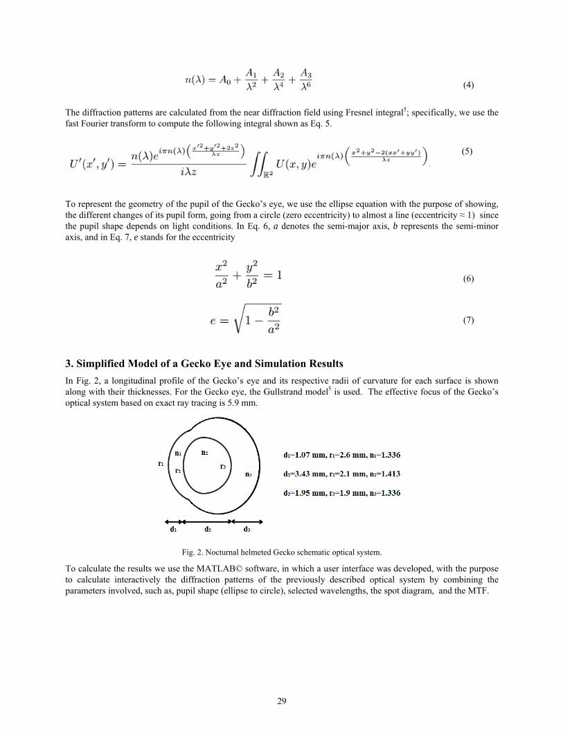
3. Simplified Model of a Gecko Eye and Simulation Results

In Fig. 2, a longitudinal profile of the Gecko’s eye and its respective radii of curvature for each surface is shown along with their thicknesses. For the Gecko eye, the Gullstrand model5 is used. The effective focus of the Gecko’s optical system based on exact ray tracing is 5.9 mm.

Fig. 2. Nocturnal helmeted Gecko schematic optical system.

To calculate the results we use the MATLAB© software, in which a user interface was developed, with the purpose to calculate interactively the diffraction patterns of the previously described optical system by combining the parameters involved, such as, pupil shape (ellipse to circle), selected wavelengths, the spot diagram, and the MTF.

29

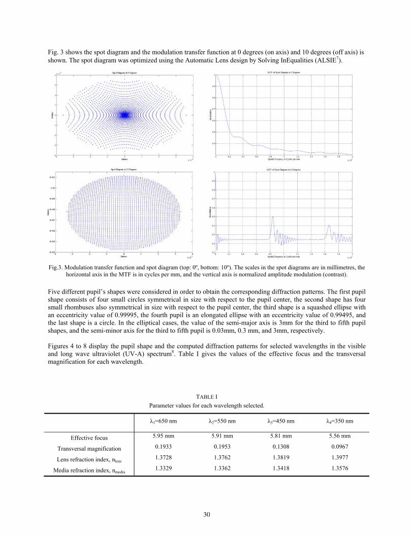
Fig. 3 shows the spot diagram and the modulation transfer function at 0 degrees (on axis) and 10 degrees (off axis) is shown. The spot diagram was optimized using the Automatic Lens design by Solving InEqualities (ALSIE7).

Fig.3. Modulation transfer function and spot diagram (top: 0º, bottom: 10º). The scales in the spot diagrams are in millimetres, the horizontal axis in the MTF is in cycles per mm, and the vertical axis is normalized amplitude modulation (contrast).

Five different pupil’s shapes were considered in order to obtain the corresponding diffraction patterns. The first pupil shape consists of four small circles symmetrical in size with respect to the pupil center, the second shape has four small rhombuses also symmetrical in size with respect to the pupil center, the third shape is a squashed ellipse with an eccentricity value of 0.99995, the fourth pupil is an elongated ellipse with an eccentricity value of 0.99495, and the last shape is a circle. In the elliptical cases, the value of the semi-major axis is 3mm for the third to fifth pupil shapes, and the semi-minor axis for the third to fifth pupil is 0.03mm, 0.3 mm, and 3mm, respectively. Figures 4 to 8 display the pupil shape and the computed diffraction patterns for selected wavelengths in the visible and long wave ultraviolet (UV-A) spectrum8. Table I gives the values of the effective focus and the transversal magnification for each wavelength.

TABLE I

Parameter values for each wavelength selected.

λ1=650 nm λ2=550 nm λ3=450 nm λ4=350 nm

Effective focus 5.95 mm 5.91 mm 5.81 mm 5.56 mm

Transversal magnification 0.1933 0.1953 0.1308 0.0967

Lens refraction index, nlens 1.3728 1.3762 1.3819 1.3977

Media refraction index, nmedia 1.3329 1.3362 1.3418 1.3576

30

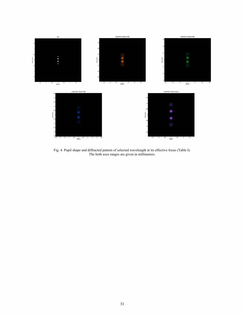
Fig. 4. Pupil shape and diffracted pattern of selected wavelength at its effective focus (Table I).

The both axes ranges are given in millimeters.

31

Fig. 5. Pupil shape and diffracted pattern of selected wavelength at its effective focus (Table I); Both axes are given in mm.

Fig. 6. Pupil shape and diffracted pattern of selected wavelength at its effective focus (Table I); Both axes are given in mm.

32

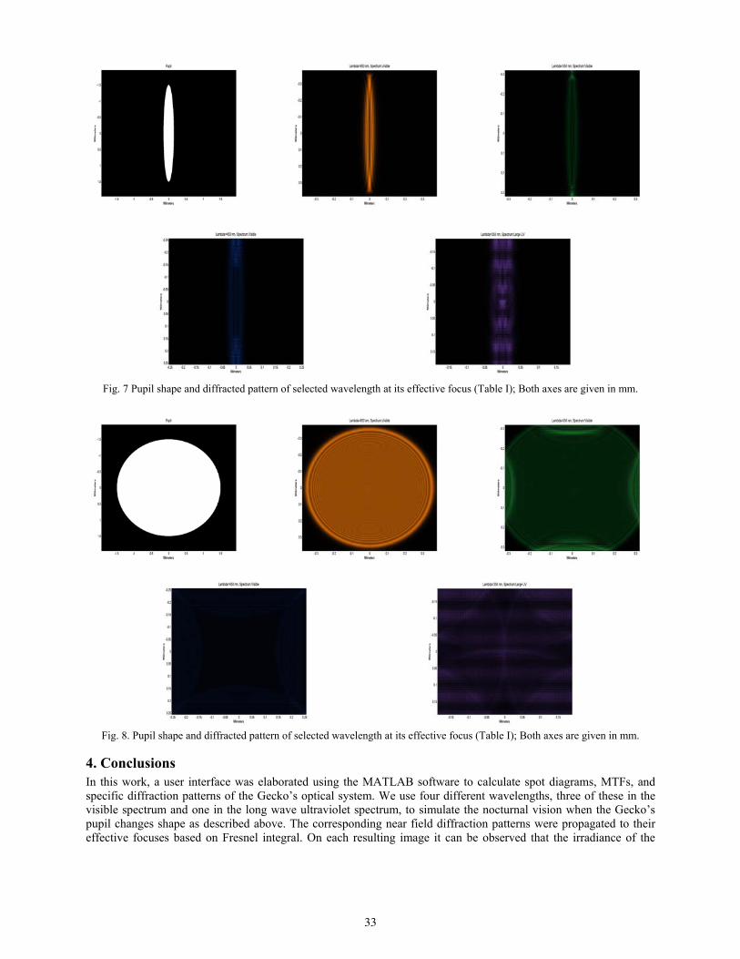
Fig. 7 Pupil shape and diffracted pattern of selected wavelength at its effective focus (Table I); Both axes are given in mm.

Fig. 8. Pupil shape and diffracted pattern of selected wavelength at its effective focus (Table I); Both axes are given in mm.

4. Conclusions In this work, a user interface was elaborated using the MATLAB software to calculate spot diagrams, MTFs, and specific diffraction patterns of the Gecko’s optical system. We use four different wavelengths, three of these in the visible spectrum and one in the long wave ultraviolet spectrum, to simulate the nocturnal vision when the Gecko’s pupil changes shape as described above. The corresponding near field diffraction patterns were propagated to their effective focuses based on Fresnel integral. On each resulting image it can be observed that the irradiance of the

33

diffraction patterns are more constant in the paraxial zone for greater wavelengths. Hence, the Gecko’s nocturnal vision system maintains pupil shape uniformity for greater wavelengths, since at lower wavelengths the irradiance is more dispersed. Also, we remark that the MTF shows poor spatial resolution. However, aforementioned limitation is compensated by its capacity to see in color under dim light.

Acknowledgements

Francisco J. Renero C. and Gonzalo Urcid S. (No. 22036) are grateful with the National Research System (SNI-CONACYT) for partial financial support. Luis David Lara Rodríguez and Elizabeth López Meléndez thank the National Council of Science and Technology (CONACYT) for doctoral scholarship with CVU No 332238 and CVU No.332355, respectively.

34

Electromechanical ruling translator system for a Dual-Aperture Common-Path Interferometer implementation

A. Barcelata-Pinzon (1), C. Meneses-Fabian (2), R. Juárez-Salazar (3) C. Robledo-Sánchez (2), J.L.

Muñoz-Mata (1), R.I. Álvarez-Tamayo (4), M. Durán-Sánchez (4), E. Barojas-Gutiérrez (2) N. Gallegos-Alegría (1)

1. Universidad Tecnológica de Puebla, México.

2. Benemérita Universidad Autónoma de Puebla, México. 3. Instituto Tecnológico de Teziutlán, México.

4. Instituto Nacional de Astrofísica Óptica y Electrónica, México. Corresponding author email: lafrecuenci@hotmail.com

ABSTRACT:

An electromechanical grid translator system for a Dual- Aperture Common-Path Interferometer (DACPI) implementation is presented. Electromechanical actuators in the field of optics are widely used because provide more accurate measuring especially in the phase-shifting process. DACPI is a robust and stable interferometric system which typically performs phase-shifts by ruling transverse displacements to the optical axis. In this work, a low precision stepper motor controlled by computer is adapted to a micrometer screw in order to achieve transverse displacements around 2 linear microns and get equally spaced phase shifts. Analytic explanation and experimental results are presented. Key words: electromechanical, actuator,interferometry,phase-shifting.

REFERENCES AND LINKS [1]C. Meneses-Fabian, G. Rodriguez-Zurita, J. F. Vazquez-Castillo, C. Robledo-Sanchez, V. Arrizón, “Common-path phase-shifting interferometer with binary grating” Opt. Comm. 264, 13-17 (2006) [2] Barcelata-Pinzon, A., Meneses-Fabian, C., Moreno-Alvarez, L., and Pastrana-Sanchez, R., “Common-path speckle interferometer for phase objects studies," Optics Communications 304(0), 153-157 (2013). [3] D. D. Verhoeven, P. V. Farrell, "Speckle interferometry in transparent media," App. Opt. 25, 903-906 (1986) [4] A. Dyrseth, R. Spooren, “Measuring mixing dyamics of transparent fluids with electronic speckle pattern interferometry” App. Opt. 36, 6171-6177 (1997) [5] P. Carré, Installation et utilisation du comparateur photoélectrique et interférentiel du Bureau International des Poids et Mesures” Metrologia 2 13 (1966) [6] C. Meneses-Fabian, G. Rodriguez-Zurita, “Optical tomography of transparent objects with phase-shifting interferometry and stepwise-shifted Ronchi ruling” J. Opt. Soc. Am. 23, 298-305 (2006) [7] Cruz Meneses-Fabian, Gustavo Rodriguez-Zurita, Ramon Rodriguez-Vera, Jose F Vazquez-Castillo, “Optical tomography with parallel projection differences and Electronic Speckle Pattern Interferometry” Optics Communications, 228, 201-210 (2003) [8] V. Arrizón, D. Sánchez-de-la-Llave, “Common-path interferometry with one-dimensional periodic filters” Opt Lett. 29, 141-143. (2004) [9] K. Creath, “Phase-shifting speckle interferometry”, App. Opt, 24 3053-3058, (1985). [10] Rigoberto Juarez-Salazar, Carlos Robledo-Sanchez, Cruz Meneses-Fabian, Gustavo Rodriguez-Zurita, Fermin Guerrero Sanchez, and Antonio Barcelata-Pinzon, “Automatic real-time generalized phase-shifting interferometry to process interferograms with spatio-temporal visibility” Proc. of SPIE Vol. 8785 878542-1 (2013)

35

1. Introduction Dual-Aperture Common-Path Interferometer (DACPI) is a very well suited interferometric system. The interferometer consists of a telecentric, 4f-Fourier imaging system with two windows in the object plane and a binary ruling as a spatial filter [1]. This kind of interferometer is very robust and has high mechanical stability because the two arms travel by the same path and therefore by the same optical components, thus the aberrations and temporal variations are compensated. Due to its high stability, this type of interferometer has recently been implemented for analysis of transparent objects using the Electronic Speckle Pattern Interferometry (ESPI) [2] technique and it has been possible to determine physical magnitudes like flow, refraction index, and temperature, among others [2-4]. For DACPI, phase stepping is usually achieved out by Ronchi ruling translation placed at Fourier plane which is operated manually or in some cases by an electromechanical actuator through a micrometer screw with typical resolutions around 10 m [2] and for some systems it is then necessary that the shifts are equally spaced [5] and that displacements are short as possible to better control of the phase amount to be introduced. When the ruling translation process is done manually, the system becomes more sensitive to parallax errors and it becomes practically impossible to get equally spaced phase-shifts between them. Electromechanical actuators provide accuracy, linearity and equally spaced phase-shifting due its electronic control and mechanical [1,6] but, in most cases, the implementation of such systems is expensive and requires certain conditions to be carried out. This paper presents an alternative process for phase-shifting adapting a low resolution stepper motor to a ruling translation system in a DACPI in order to obtain equally spaced steps with a ruling linear translation resolution around 20 nm and generate short phase steps between consecutive interference patterns. The goal of this work is propose and implement an inexpensive and easily implemented system to generate the steps. Experimental results and analytic explanation are shown below. 2. Theoretical Model: Dual-aperture common-path interferometer DACPI [1] is built on a 4 f imaging system consisting of two apertures in the object plane and a Ronchi ruling in the

Fourier plane (Fig. 1). In one aperture a phase object is placed, serving as a probe arm, while a second object is left free of obstacles, serving as a reference arm. If a collimated laser beam, lineally polarized, monochromatic with wavelength , illuminates this system, the field leaving from the windows is described by

0 0 0 0 0

1 1 1 1 1, , , , , exp ,

2 2 2 2 2A R Ot x y w x x y A x x y w x x y A x x y i x x y , (1)

where ( , ) rect( )rect( )w ww x y x a y b represents a rectangular window of sides wa and wb , with rect(...) denoting the

rectangle function; 0x is the distance of separation between the windows A and B; RA and OA are the amplitudes of

the beams leaving from the windows; the phase function is due to the phase object; and 1i is the maginary

unit. At the frequency plane, a Ronchi ruling of period pu with a fill factor of 1/2 and displaced by a distance du is

described by

, rect

2p d

n p

nR , (2)

where , ,u f v f , p pu f , d du f are spatial frequencies and f is the focal distance of the

lenses. The system’s impulse response given by the inverse Fourier-transform is written as

1 1

, sinc exp 2 ,2 2

d

n p p

fur x y n i n x n y

u u. (3)

36

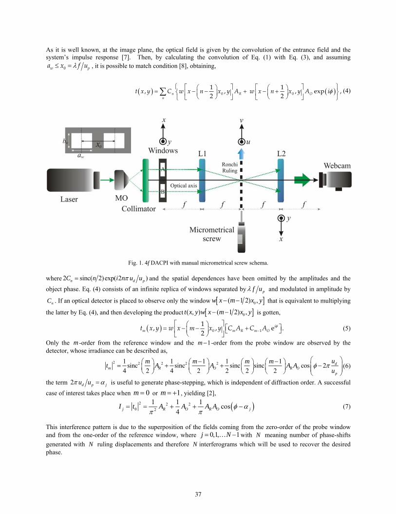
As it is well known, at the image plane, the optical field is given by the convolution of the entrance field and the system’s impulse response [7]. Then, by calculating the convolution of Eq. (1) with Eq. (3), and assuming

0w pa x f u , it is possible to match condition [8], obtaining,

0 0

1 1, , , exp ,

2 2n R On

t x y C w x n x y A w x n x y A i (4)

Fig. 1. 4f DACPI with manual micrometrical screw schema. where 2 sinc( 2)exp( 2 )n d pC n i n u u and the spatial dependences have been omitted by the amplitudes and the

object phase. Eq. (4) consists of an infinite replica of windows separated by pf u and modulated in amplitude by

nC . If an optical detector is placed to observe only the window 0( 1 2) ,w x m x y that is equivalent to multiplying

the latter by Eq. (4), and then developing the product 0( , ) ( 1 2) ,t x y w x m x y is gotten,

0 1

1, , e .

2i

m m R m Ot x y w x m x y C A C A (5)

Only the m -order from the reference window and the 1m -order from the probe window are observed by the detector, whose irradiance can be described as,

2 2 2 2 21 1 1 1 1sinc sinc sinc sinc cos 2

4 2 4 2 2 2 2d

m R O R Op

um m m mt A A A A

u

(6)

the term 2 d p ju u is useful to generate phase-stepping, which is independent of diffraction order. A successful

case of interest takes place when 0m or 1m , yielding [2],

2 2 20 2

1 1 1cos

4j R O R O jI t A A A A

(7)

This interference pattern is due to the superposition of the fields coming from the zero-order of the probe window and from the one-order of the reference window, where 0,1, 1j N with N meaning number of phase-shifts

generated with N ruling displacements and therefore N interferograms which will be used to recover the desired phase.

37

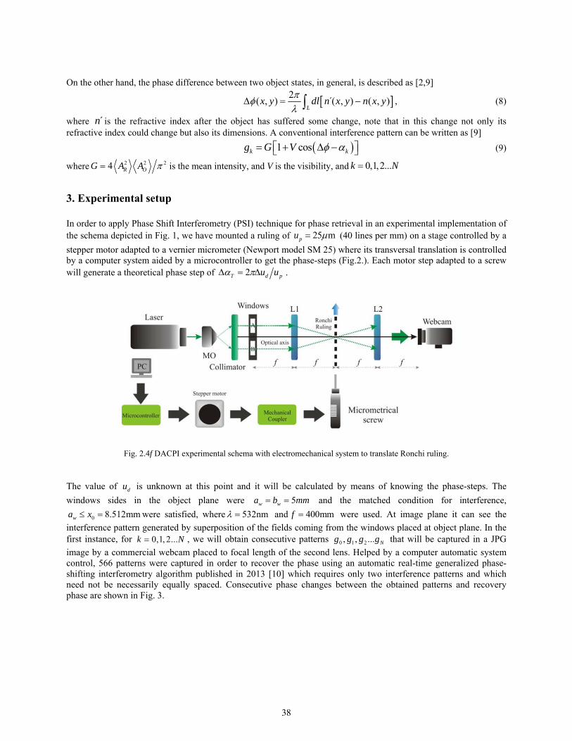
On the other hand, the phase difference between two object states, in general, is described as [2,9]

2( , ) ´( , ) ( , )

Lx y dl n x y n x y

, (8)

where ´n is the refractive index after the object has suffered some change, note that in this change not only its refractive index could change but also its dimensions. A conventional interference pattern can be written as [9]

1 cosk kg G V (9)

where 2 2 24 R OG A A is the mean intensity, and V is the visibility, and 0,1,2...k N

3. Experimental setup In order to apply Phase Shift Interferometry (PSI) technique for phase retrieval in an experimental implementation of the schema depicted in Fig. 1, we have mounted a ruling of 25 mpu (40 lines per mm) on a stage controlled by a

stepper motor adapted to a vernier micrometer (Newport model SM 25) where its transversal translation is controlled by a computer system aided by a microcontroller to get the phase-steps (Fig.2.). Each motor step adapted to a screw will generate a theoretical phase step of 2T d pu u .

Fig. 2.4f DACPI experimental schema with electromechanical system to translate Ronchi ruling. The value of du is unknown at this point and it will be calculated by means of knowing the phase-steps. The

windows sides in the object plane were 5w wa b mm and the matched condition for interference,

0 8.512mmwa x were satisfied, where 532nm and 400mmf were used. At image plane it can see the

interference pattern generated by superposition of the fields coming from the windows placed at object plane. In the first instance, for 0,1, 2...k N , we will obtain consecutive patterns 0 1 2, , ... Ng g g g that will be captured in a JPG

image by a commercial webcam placed to focal length of the second lens. Helped by a computer automatic system control, 566 patterns were captured in order to recover the phase using an automatic real-time generalized phase-shifting interferometry algorithm published in 2013 [10] which requires only two interference patterns and which need not be necessarily equally spaced. Consecutive phase changes between the obtained patterns and recovery phase are shown in Fig. 3.

38

Fig. 3. a) Reference interference pattern, b) Consecutive interference pattern, c)Recovery phase, d) Graph to show the phase values versus N steps.

The average phase recovered obtained between consecutive displacements is 0.31 rad such that the actuator

linear average displacement is (0.31 )(25 ) 2 1.23du rad m m . Compared with 4.947 rad obtained for

the same experimental setup using a 10 microns standard micrometer device of resolution manually, the electromechanical actuator gets phase-shifts 10 times smaller than manually operation [2]. The average standard deviation of the global results is 0.155 wich indicates acceptable data dispersion compared with reported values for the same screw and DACPI system [2] and for this preliminary implementation. Steps fluctuations are due to the coupling device between the motor and the micrometer screw presents pitching in its performance by its construction because the fastening system is achieved in manually form (see Fig.4. ) but it is designable and will be improved in future work.

Fig.4. a) Mechanical coupler frontal view, b) Mechanical coupler side view.

4. Conclusions We have presented an electromechanical grid translator system for a Dual-Aperture Common-Path Interferometer in order to obtain electromechanical ruling displacements at the Fourier plane to generate equally spaced and small

39

phase-shiftings. At image plane, 566 interference patterns were captured with a commercial webcam, same that were processed later by means of an automatic real-time generalized phase-shifting interferometry algorithm obtaining

0.31 rad between consecutive steps, achieving 10 times smaller phase-shifts than manually operation and on average, equally spaced shifts that was initially persecuted. This system results in an inexpensive and easily implementation device to perform and add to a DACPI to apply in several optical analysis. As a side note, it is worth mentioning that the device was developed in the research department of Mechatronics at the Universidad Tecnológica de Puebla and implemented for testing in the Applied Optics Lab at the Physical-Mathematics Department at the Benemérita Universidad Autónoma de Puebla. Acknowledgements

A. Barcelata-Pinzon thanks support PROMEP key UTPUE-CA-13 for the realization of this work and to Mechatronics department at Universidad Tecnológica de Puebla as well as Applied Optics Lab at the Physical-Mathematics Department at the Benemérita Universidad Autónoma de Puebla.

40

Constant of absorbance of latex in an aqueous solution

L. Torres Quiñonez, A. Acevedo Carrera, F. Moreno López, S. Estrada Dorado (1)

1. México, Universidad de Sonora Corresponding author email:

lutock352@gmail.com, albetoman@hotmail.com, xerk.kun@gmail.com, sandinuco.ruco@gmail.com

ABSTRACT:

We dissolve five microliters of a latex microsphere suspension, in ten milliliters of water. This is called the master solution. Then we make sixteen samples dissolving part of the master solution in ten milliliters of water, obtaining different concentrations. With a Pasco sensor we measure the intensity of the laser through clean water and the samples obtaining pairs of data, intensity and concentration. The data show us the behavior of graphic intensity-concentration. Knowing that the absorbance nature is logarithmic we can make a straight fit and a logarithmic fit, the first one in accordance to the Beer’s Law and let us calculate the constant of absorbance, the second one to compare the realistic absorbance nature with the results.

REFERENCES AND LINKS [1] Bmglabtech.com, (2015). Absorbancia - Modos de Detección - Tecnológico - BMG LABTECH. [online]

Available at: http://www.bmglabtech.com/es/tecnologico/modos-de-deteccion/absorbancia/ [Accessed 30 Jul. 2015].

[2] DiLisi G. A., DiLisi L. A., Winters C. M., Peckinpaugh K. M. Got milk? A Beer's Law Experiment, John Carroll University, University Hts., OH, Parker Hannifin Corp. - Nichols Airborne Division, Elyria, OH, Beaumont School for Girls, Cleveland Hts., OH

1. Introduction

Taking into account the properties of the materials to reflect and absorb light we suspended latex particles in a solution of water. Measure the absorbance of the solution in the process and find a material constant. For this we will rely on the definition of absorbance and Beer's law. The importance of the constant is that knowing it, we would be able to calculate the concentration of a material from its absorbance.

2. Theorical framework

Absorbance is defined in everyday terms as the amount of light that is absorbed by a medium, when a laser impinged it. In this case we will focus on an aqueous sample of colloid particles. Although it is also possible with other substances. In a more academic form it is known as a logarithmic relationship between the intensity incident on the sample and the intensity of that light coming out of the sample. This is because when light of a certain wavelength on

41

a sample, a part of the incident light is absorbed. The light not absorbed moves on and passes through the sample. Importantly, the amount of light that is absorbed differs with different wavelengths and can lead to miscalculations if the same wavelength is not used to conduct an experiment. Also the amount of light absorbed by the sample depends on its concentration. At low concentrations the relationship between absorbance and concentration is known as Beer's law. This law takes into account three factors, concentration, step width that will cross the beam and an intrinsic constant of the material that has been diluted in the sample. With these three factors we will find the relationship of Beer. Considering a light beam of uniform area and intensity I0 incident, which headed a clear liquid that contains suspended particles. This suspension is characterized by two parameters, concentration C, and the distance the laser L shows. Considering differential as dx beam path, the number of particles that will be in contact with the laser is: ACdx (1)

If each particle has a cross-sectional area α, we can see that the total area of absorbance by the beam is:

dA= αCAdx (2)

Therefore, the change of intensity of the beam as it progresses through the solution is:

(3)

Replacing the value given in equation we get:

(4)

Integrating along the entire length it is obtained:

(5)

As mentioned this equation is valid only at low concentrations. Because the particles at high concentrations are so close together that the light is scattered by other particles and redispersed, so it is expected to have deviations from the model.

42

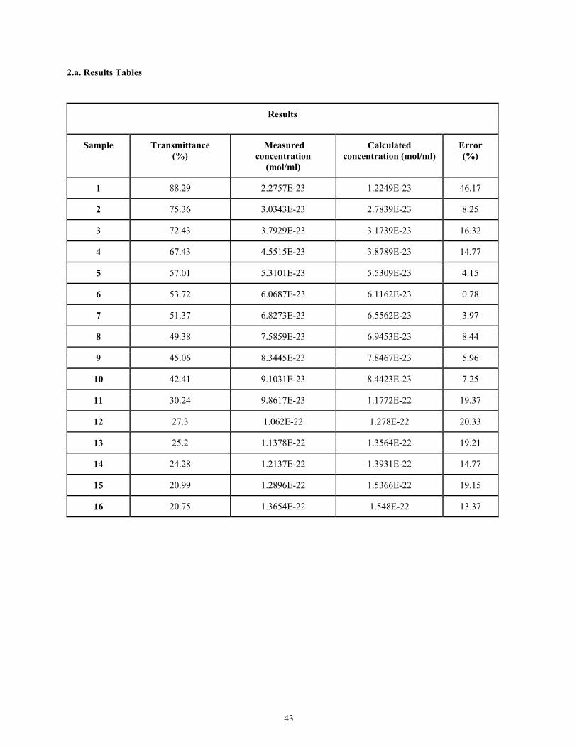
2.a. Results Tables

Results

Sample Transmittance (%)

Measured concentration

(mol/ml)

Calculated concentration (mol/ml)

Error(%)

1 88.29 2.2757E-23 1.2249E-23 46.17

2 75.36 3.0343E-23 2.7839E-23 8.25

3 72.43 3.7929E-23 3.1739E-23 16.32

4 67.43 4.5515E-23 3.8789E-23 14.77

5 57.01 5.3101E-23 5.5309E-23 4.15

6 53.72 6.0687E-23 6.1162E-23 0.78

7 51.37 6.8273E-23 6.5562E-23 3.97

8 49.38 7.5859E-23 6.9453E-23 8.44

9 45.06 8.3445E-23 7.8467E-23 5.96

10 42.41 9.1031E-23 8.4423E-23 7.25

11 30.24 9.8617E-23 1.1772E-22 19.37

12 27.3 1.062E-22 1.278E-22 20.33

13 25.2 1.1378E-22 1.3564E-22 19.21

14 24.28 1.2137E-22 1.3931E-22 14.77

15 20.99 1.2896E-22 1.5366E-22 19.15

16 20.75 1.3654E-22 1.548E-22 13.37

43

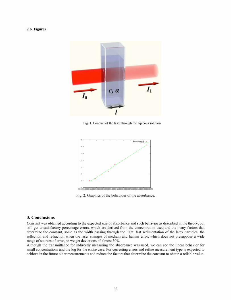
2.b. Figures

Fig. 1. Conduct of the laser through the aqueous solution.

Fig. 2. Graphics of the behaviour of the absorbance.

3. Conclusions Constant was obtained according to the expected size of absorbance and such behavior as described in the theory, but still get unsatisfactory percentage errors, which are derived from the concentration used and the many factors that determine the constant, some as the width passing through the light, fast sedimentation of the latex particles, the reflection and refraction when the laser changes of medium and human error, which does not presuppose a wide range of sources of error, so we get deviations of almost 50%. Although the transmittance for indirectly measuring the absorbance was used, we can see the linear behavior for small concentrations and the log for the entire case. For correcting errors and refine measurement type is expected to achieve in the future older measurements and reduce the factors that determine the constant to obtain a reliable value.

44

A study of the effects of phase and intensity noise on the measurements obtained from the structured light projection technique with temporal phase

unwrapping

G. Frausto-Rea and A. Dávila

Centro de Investigaciones en Óptica, México gloriafrausto@cio.mx

ABSTRACT:

Most of the structured light projection techniques can measure phase that is related to the 3D shape of the object under analysis. However, the spatial phase unwrapping usually fails when there are shades, obstructions, glares and intensity noise. To solve these problems, a proven technique that is immune to spatial phase errors is the temporal phase unwrapping technique (TPU). This technique allows phase unwrapping, even when spatial under-sampling of phase occurs, and when isolated objects are inspected simultaneously. However, its performance when noise is introduced either in intensity or phase is still unknown for particular applications such as the structured light projection techniques. In this work, a study of the TPU performance under phase and intensity errors is presented. It is shown that the TPU technique is able to provide correct measurements even when phase and intensity errors of a given magnitude are introduced. 3D shape measurement of mechanical objects is presented to show the magnitude of shape errors obtained in a typical structured light projection system.

Key words: structured light projection, temporal phase unwrapping.

REFERENCES AND LINKS [1] Huntley, J.M., y Sandler, H. (1993). Temporal phase-unwrapping algorithm for automated interferogram analysis. Appl. Opt., 32 (17), 3047-3052. [2] Zhao, H., Chen, y W., Tan, Y. (1994). Phase-unwrapping algorithm for the measurement of three-dimensional object shapes. Appl. Opt., 33 (20), 4497-4500. [3] Huntley, J.M., y Saldner, H.O., (1997). Shape measurement by temporal phase unwrapping: comparison of unwrapping algorithms. Meas. Sci. Tecnol., 8, 986-992. [4] Huntley, J.M., y Saldner, H.O. (1997). Shape measurement by temporal phase unwrapping and spatial light modulator-based fringe projector. Proceedings SPIE, 3100, 185-192. [5] Huntley, J.M., y Saldner, H.O., (1997). Error-reduction methods for shape measurement by temporal phase unwrapping. J. Opt. Soc. Am., 14 (12), 3188-3196. [6] Saldner, H.O., y Huntley, J.M. (1997). Temporal phase unwrapping: application to surface profiling of discontinuous objects. Appl. Opt., 36 (13), 2770-2775. [7] Van den Doel, L. R. y Van Vliet, L. J. (2001). Temporal phase-unwrapping algorithm for dynamic interference pattern analysis in interference-contrast microscopy. Appl. Opt., 40 (23), 4487-4500. [8] Peng, X., Yang, Z., y Niu, H. (2003). Multi-resolution reconstruction of 3-D image with modified temporal unwrapping algorithm. Opt. Commun., 224, 35-44. [9] Salfity, M.F., Huntley, J.M., Graves, M.J., Marklund, O., Cusack, R., y Beauregard, D. A. (2004). 3-D and 4-D phase unwrapping methods applied to phase contrast magnetic resonance velocity imaging. ICEM12-12th International Conference on Experimental Mechanics.

45

[10] Zhang, S., Li, X., y Yau, S.T. (2007). Multilevel quality-guided phase unwrapping algorithm for real-time three-dimensional shape reconstruction. Appl. Opt., 46 (1), 50-57. [11] Tian, J., Peng, X., y Zhao, X. (2008). A generalized temporal phase unwrapping algorithm for three-dimensional profilometry. Optics and lasers engineering, 46, 336-342. [12] Pribanić, T., Mrvoš, S., y Salvi, J. (2010). Efficient multiple phase shift pattern for dense 3D acquisition in structured light scanning. Image and Vision Computing, 28, 1255-1266. [13] Yong, L., Huang, D., Yong, J. (2012). Flexible error-reduction method for shape measurement by temporal phase unwrapping: phase averaging method. Appl. Opt., 51 (21), 4945-4953. [14] Fu, Y., y Luo, Q. (2011). Fringe projection profilometry based on a novel phase shift method. Optics Express,

19 (22), 21739-21747.

[15] Huntley, J.M., y Saldner, H.O., (1997). Error-reduction methods for shape measurement by temporal phase unwrapping. J. Opt. Soc. Am., 14 (12), 3188-3196.

1. Introduction The first attempts to obtain the shape of an object using the temporal phase unwrapping technique date from 1993, where Huntley [1] proposed a new algorithm for phase unwrapping using interference fringes projected over an object. The novel idea was stated such as each pixel phase was measured as a function of time. Unwrapping is then carried out along the time axis for each pixel independently of the others. So the boundaries and regions with poor signal to noise ratio, does not contribute or influence the neighbors with strong signals. In 1994 Zhao [2] presented a phase unwrapping algorithm in which two phase maps were needed, and the fringe orders were assigned using the phase map with lower phase modulation and the phase unwrapping of each point was achieved independently even in the presence of discontinuities. Later, Huntley and Saldner [3] (1997) proposed two TPU algorithms: the first operates using a time-sequence of phase maps produced by a linear change in the spatial frequency of fringe patterns, the second uses exponentially changes of the spatial frequency of the fringe patterns. One of the main advantages of the TPU, is that the absolute profile is obtained even in the presence of discontinuous surfaces. In 1997 Huntley and Saldner [4] investigated several modifications to the basic TPU such as the exponential decrement in the number of fringes. In the same year, Huntley and Saldner [5] showed several methods to reduce the error in measurement of shapes using the temporal phase unwrapping. Their first method used an exponentially growing sequence of values of phase, another method was proposed when the phase sequence has noise, and a least squares fit was used for noise reduction, additionally other methods used the main peak position obtained after a Fourier transform of the fringe patterns sequence to provide range data directly; this last approach has shown low measurements error and high reliability. Combining fringe projection methods with phase shifting methods and the temporal phase unwrapping produced a more effective method of surface profile measurement [6] (1997). In 2001, Van den Doel and van Vliet [7] developed a temporal phase unwrapping algorithm to analyze dynamic interference patterns from interference-contrast microscopy using vials micromachines of picoliters. They made a study of the dynamic behavior of evaporating liquid in sub-nanoliter regimes that required a fluid volume properly sampled in time, as well as in space. In 2003 Peng, Yang and Niu [8] in order to increase TPU efficiency, proposed initial conditions for the TPU algorithm. As the phase contrast in magnetic resonance imaging produces a linear relationship between blood velocity and the phase shifting of the magnetic resonance signal, in 2004 a method of 3D TPU was applied to magnetic resonance imaging by Salfity et al. [9]. In 2007, Zhang, Li and Yau [10] generated a quality map based in the gradient of the phase map, and with multilevel thresholding they unwrapped the phase level by level. Similarly, Zhang et al. [11] proposed phase unwrapping algorithms which handle the errors of these techniques, with Tian, Peng and Zhao [103] (2008) proposing a general algorithm, which eliminates some limitations imposed on the sequence of fringes for the classic algorithm. In 2010, the work of Pribanić, Mrvoš and Salvi [12] introduced a method of multiple phase shifts to unwrap a phase, for neutral and colored objects using only two phase maps from eight shifted fringe patterns, with two additional patterns used as a reference to facilitate the detection of shadows and occluded regions. In 2012 Yong et al. [13] proposed a method of averaging phase to reduce errors caused by camera noise or nonlinearity. Their method used an additional fringe sequence next to the highest density fringe used for improved data processing he shows that nonlinear errors are eliminated, and the phase measurement is more accurate than other methods.

46

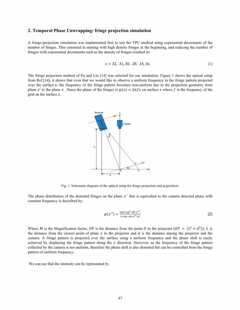
2. Temporal Phase Unwrapping: fringe projection simulation

A fringe-projection simulation was implemented first to test the TPU method using exponential decrements of the number of fringes. This consisted in starting with high density fringes at the beginning, and reducing the number of fringes with exponential decrements such as the density of fringes resulted in:

32, 31, 30, 28, 24, 16. (1)

The fringe projection method of Fu and Liu [14] was selected for our simulation. Figure 1 shows the optical setup from Ref.[14], it shows that even that we would like to observe a uniform frequency in the fringe pattern projected over the surface , the frequency of the fringe pattern becomes non-uniform due to the projection geometry from plane ′ to the plane . Since the phase of the fringes is 2 on surface where is the frequency of the grid on the surface .

Fig. 1. Schematic diagram of the optical setup for fringe projection and acquisition.

The phase distribution of the distorted fringes on the plane ´´ that is equivalent to the camera detected phase with constant frequency is described by:

′∗ ∗ ∗ .

∗ ∗ ∗ (2)

Where is the Magnification factor, is the distance from the point to the projector ( , L is the distance from the closest point of plane to the projector and is the distance among the projector and the camera. A fringe pattern is projected over the surface using a uniform frequency and the phase shift is easily achieved by displacing the fringe pattern along the direction. However, as the frequency of the fringe pattern collected by the camera is not uniform, therefore the phase shift is also distorted but can be controlled from the fringe pattern of uniform frequency.

We can see that the intensity can be represented by

47

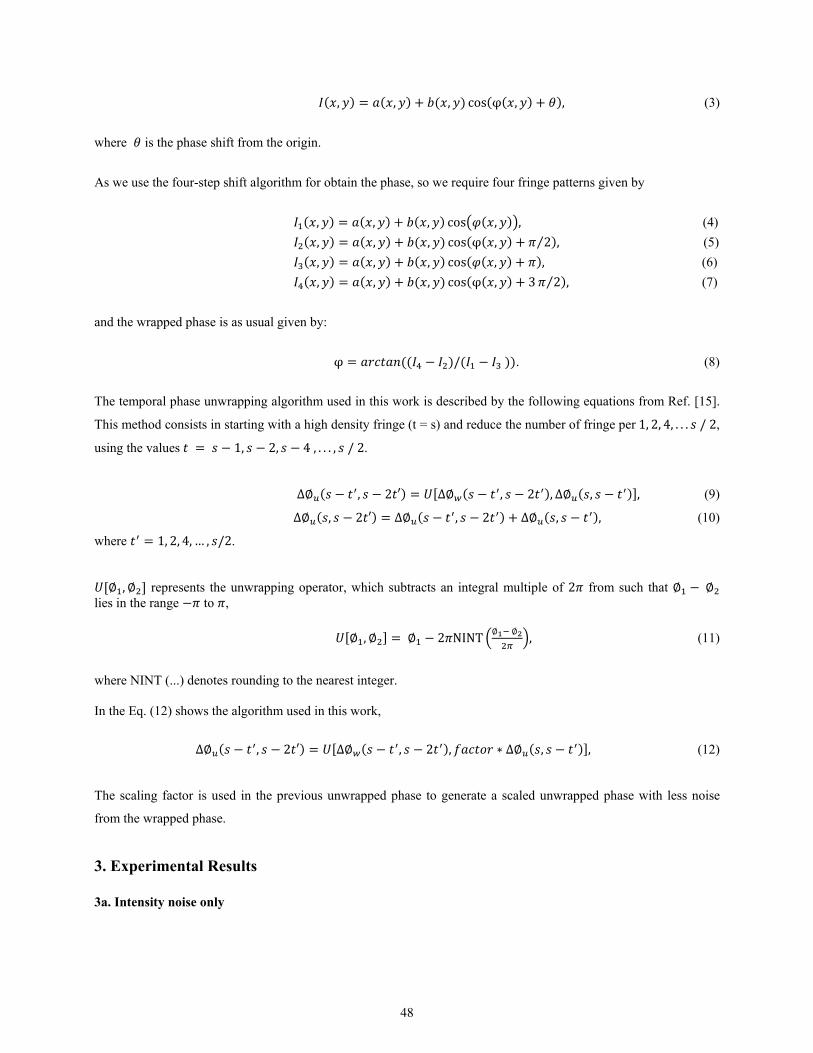
, , , cos φ , , (3)

where is the phase shift from the origin.

As we use the four-step shift algorithm for obtain the phase, so we require four fringe patterns given by

, , , cos , ,(4)

, , , cos φ , 2⁄ , (5)

, , , cos , , (6)

, , , cos φ , 3 2⁄ , (7)

and the wrapped phase is as usual given by:

φ / . (8)

The temporal phase unwrapping algorithm used in this work is described by the following equations from Ref. [15].

This method consists in starting with a high density fringe (t = s) and reduce the number of fringe per1, 2, 4, . . . /2,

using the values 1, 2, 4, . . . , /2.

∆∅ , 2 ′ ∆∅ , 2 , ∆∅ , , (9)

∆∅ , 2 ′ ∆∅ , 2 ∆∅ , , (10)

where 1, 2, 4, … , /2.

∅ , ∅ represents the unwrapping operator, which subtracts an integral multiple of 2 from such that ∅ ∅ lies in the range to ,

∅ , ∅ ∅ 2 NINT∅ ∅

, (11)

where NINT (...) denotes rounding to the nearest integer. In the Eq. (12) shows the algorithm used in this work,

∆∅ , 2 ′ ∆∅ , 2 , ∗ ∆∅ , , (12)

The scaling factor is used in the previous unwrapped phase to generate a scaled unwrapped phase with less noise

from the wrapped phase.

3. Experimental Results 3a. Intensity noise only

48

A Gaussian phase function was simulated as an object to test our algorithm in the presence of noise, the fringe projection phase of Eq. (2) was added to the Gaussian phase to complete our simulation. In Figure 2 we can see the result of the reconstruction using temporal phase unwrapping, the reconstruction with added intensity noise up to 6.5 a.u. with 127 and 127 from Eq. 3 resulted in the same plot.

Fig. 2. Reconstruction of a Gaussian function using temporal phase unwrapping up to with intensity noise less than 6.5 a.u.

Table I shows how the intensity noise produced RMS phase error. It shows that the error is non-linear due to the random noise.

TABLE I

RMS Error in radians for intensity noise in a.u.

Intensity Noise RMS Error

0.0 0.0000

0.1 0.0020

0.2 0.0038

0.3 0.0035

0.4 0.0023

0.5 0.0080

0.6 0.0029

0.7 0.0100

0.8 0.0086

0.9 0.0025

1.0 0.0123

1.5 0.0500

2.0 0.0622

2.5 0.0326

3.0 0.0106

3.5 0.0178

4.0 0.0844

4.5 0.1332

5.0 0.0619

5.5 0.0960

6.0 0.0926

6.5 0.1339

7.0 0.1501

7.5 0.1188

8.0 0.0232

8.5 0.2213

9.0 0.0694

9.5 0.0874

10.0 0.1747

15.0 0.2715

20.0 0.3676

25.0 0.3666

30.0 0.4068

35.0 0.6399

To test the performance under large amounts of noise, in this part of the simulation, we can see that when we apply noise 6.5 a.u. the reconstruction of the Gaussian was already affected: noise peaks with values less than zero, due to re-wrapping started to appear. Figs. 3 and 4 show the erroneous peaks on the surface and below the same.

49

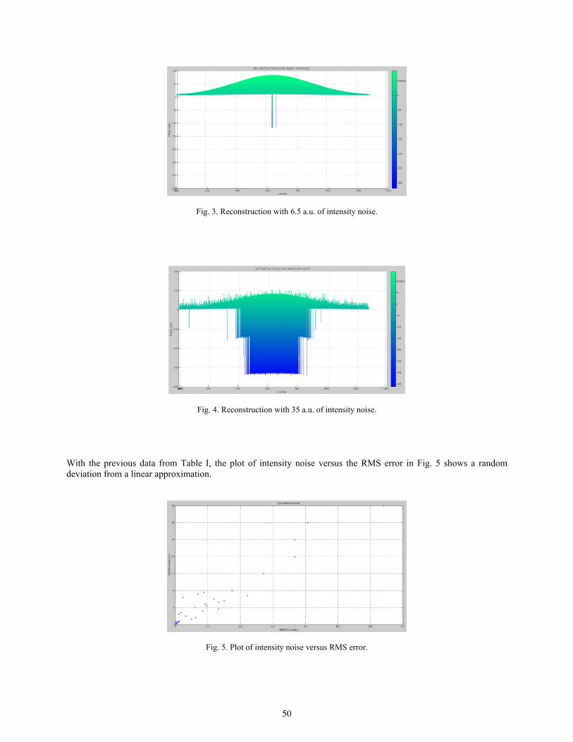
Fig. 3. Reconstruction with 6.5 a.u. of intensity noise.

Fig. 4. Reconstruction with 35 a.u. of intensity noise.

With the previous data from Table I, the plot of intensity noise versus the RMS error in Fig. 5 shows a random deviation from a linear approximation.

Fig. 5. Plot of intensity noise versus RMS error.

50

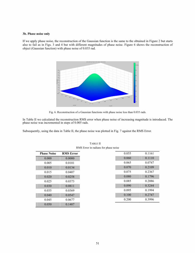
3b. Phase noise only If we apply phase noise, the reconstruction of the Gaussian function is the same to the obtained in Figure 2 but starts also to fail as in Figs. 3 and 4 but with different magnitudes of phase noise. Figure 6 shows the reconstruction of object (Gaussian function) with phase noise of 0.035 rad.

Fig. 6. Reconstruction of a Gaussian functions with phase noise less than 0.035 rads. In Table II we calculated the reconstruction RMS error when phase noise of increasing magnitude is introduced. The phase noise was incremented in steps of 0.005 rads. Subsequently, using the data in Table II, the phase noise was plotted in Fig. 7 against the RMS Error. TABLE II

RMS Error in radians for phase noise

Phase Noise RMS Error

0.000 0.0000

0.005 0.0101

0.010 0.0134

0.015 0.0407

0.020 0.0258

0.025 0.0373

0.030 0.0811

0.035 0.0369

0.040 0.0547

0.045 0.0677

0.050 0.1407

0.055 0.1161

0.060 0.1110

0.065 0.0747

0.070 0.2109

0.075 0.2367

0.080 0.1796

0.085 0.2086

0.090 0.3244

0.095 0.1994

0.100 0.2747

0.200 0.3996

51

Fig. 7. Plot of phase noise versus RMS error.

Similarly, it was observed that with some noise value will begin to see noise peaks. In this case the noise value was 0.035 (Figure (8)); and when we have a phase noise of 0.2 (Figure (9)), the peaks are on the surface and beneath the surface of the Gaussian. Finally, Fig. 10 shows a real object reconstructed using the experimental setup of Fig. 1 and the TPU technique.

Fig. 8. Gaussian reconstruction with 0.035 rad phase noise.

Fig. 9. Gaussian reconstruction with 0.2 rad phase noise.

52

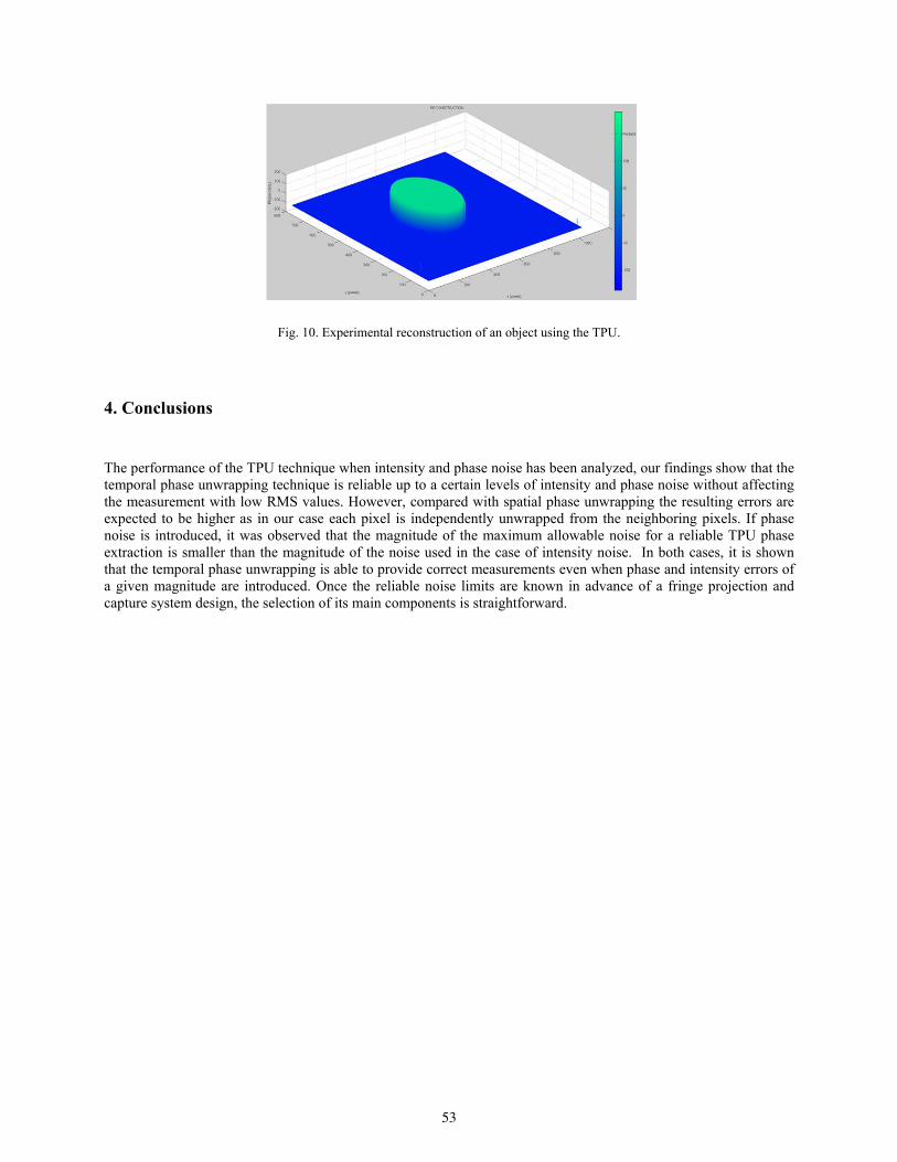
Fig. 10. Experimental reconstruction of an object using the TPU.

4. Conclusions

The performance of the TPU technique when intensity and phase noise has been analyzed, our findings show that the temporal phase unwrapping technique is reliable up to a certain levels of intensity and phase noise without affecting the measurement with low RMS values. However, compared with spatial phase unwrapping the resulting errors are expected to be higher as in our case each pixel is independently unwrapped from the neighboring pixels. If phase noise is introduced, it was observed that the magnitude of the maximum allowable noise for a reliable TPU phase extraction is smaller than the magnitude of the noise used in the case of intensity noise. In both cases, it is shown that the temporal phase unwrapping is able to provide correct measurements even when phase and intensity errors of a given magnitude are introduced. Once the reliable noise limits are known in advance of a fringe projection and capture system design, the selection of its main components is straightforward.

53

Tomographic reconstruction of asymmetrical phase objects L. R. Berriel Valdos (1) , E. de la Rosa Miranda (2), C. A. Olvera Olvera (2), J. G. Arceo Olague (2),

T. Saucedo Anaya (3), J. I. de la Rosa Vargas (2)

1. Departamento de Óptica, Instituto Nacional de Astrofísica, Óptica y Electrónica, Enrique Erro No. 1, Santa María Tonantzintla, San Andrés Cholula, C.P. 72840, Puebla, México

2. Unidad Académica de Ingeniería Eléctrica, Universidad Autónoma de Zacatecas, Antiguo Camino a la Bufa No. 1, Col. Centro. C. P. 98000, Zacatecas, Zac. México

3. Unidad Académica de Física, Universidad Autónoma de Zacatecas, Antiguo Camino a la Bufa No. 1, Col. Centro. C. P. 98000, Zacatecas, Zac. México

Corresponding author email: berval@inaoep.mx

ABSTRACT:

The number of projections needed for tomographic reconstruction of asymmetrical phase objects in the non-refractive limit is high when standard methods are used, which complicates the interferometric implementation. However, if the objects are smooth, they can be reconstructed using basis functions, minimizing the number of subject constrains projections. In this work it is shown the tomographic reconstruction of a candle flame.

Key words: Optical tomography, interferogram analysis, phase object

REFERENCES AND LINKS [1] Nadir Yilmaz, Walt Gill, A. Burl Donaldson, and Ralph E. Lucero. “Problems encountered in fluctuating flame

temperature measurements by thermocouple”. Sensors, 8(12):7882–7893, (2008).

[2] Xudong Xiao, Ishwar K. Puri, and Ajay K. Agrawal. “Temperature measurements in steady axisymmetric partially premixed flames by use of rainbow schlieren deflectometry”. Appl. Opt., 41(10):1922–1928, Apr (2002).

[3] P.M. Brisley, Gang Lu, Yong Yan, and S. Cornwell. “Three-dimensional temperature measurement of combustion flames using a single monochromatic ccd camera”. Instrumentation and Measurement, IEEE Transactions on, 54(4):1417–1421, Aug (2005).

[4] Hiroki Uchiyama, Masato Nakajima, and Shinichi Yuta. “Measurement of flame temperature distribution by ir emission computed tomography”. Appl. Opt., 24(23):4111–4116, Dec (1985).

[5] Juan C. Aguilar, Luis Raul Berriel-Valdos, and Jose Felix Aguilar. “Measuring of temperatures of a candle flame using four multidirectional point-di�raction interferometers”. Optical Engineering, 52(10):104103– 104103, (2013).

[6] C. Alvarez-Herrera, D. Moreno-Hernández, and B. Barrientos-García. “Temperature measurement of an axisymmetric flame by using a schlieren system”. Journal of Optics A: Pure and Applied Optics, 10(10):104014, oct (2008).

[7] Charles M. Vest. Holographic Interferometry. John Wiley & Sons, New York, (1979). [8] K. J. Gasvik. Optical Metrology. Wiley, New York, (1987). [9] Mitsuo Takeda, Hideki Ina, and Seiji Kobayashi. “Fourier-Transform Method of Fringe-Pattern Analysis for

Computer-Based Topography and Interferometry”. Journal of Optical Society of America A, 72,156–159, (1981).

[10] D. Malacara, M. Servín, and Z. Malacara. Interferogram Analysis for Optical Testing. Marcel-Dekker, Inc.,

54

New York, (1998). [11] Jesús Villa, Ismael de la Rosa Gerardo Miramontes, and Juan Antonio Quiroga. “Phase recovery from a single

fringe pattern using an orientational vector field regularized estimator”. Journal of Optical Society of America A, 22, 2766–2773, (2005).

[12] L. Guerriero, G. Nico, G. Pasquariello, and S. Stramaglia. “New regularization scheme for phase unwrapping”. Applied Optics, 37(14):3053–3058, (1998).

[13] M. Rivera and J. L. Marroquin. “Half-quadratic cost functions for phase unwrapping”. Optics Letters, 29(5):504–506, (2004).

[14] B. Ströbel. “Processing of interferometric phase maps as complex-valued phasor images”. Applied Optics, 35:2192–2198, (1996).

[15] D.C. Ghiglia and M.D. Pritt. Two-dimensional phase unwrapping: theory, algorithms, and software. Wiley-Interscience publication. Wiley, (1998).

[16] B. R. Hunt. “Matrix formulation of the reconstruction of phase values from phase di�erences”. J. Opt. Soc. Am., 69(3):393–399, Mar (1979).

[17] Dennis C. Ghiglia and Louis A. Romero. “Robust Two-Dimensional Weighted and Unweighted, Phase Unwrapping for Uses Fast Transform and Iterative Methods”. Journal of Optical Society of America A, 11:107–117, (1994).

[18] S. R. Deans. The Radon Transform and Some of its Applications. Wiley, New York, first edition, 1983. [19 R.M. Lewitt. “Reconstruction algorithms: Transform methods”. Proceedings of the IEEE, 71(3):390–408, March

(1983). [20] H.J. Scudder. “Introduction to computer aided tomography”. Proceedings of the IEEE, 66(6):628–637, June

(1978). [21] A. K. Jain. Fundamental of Digital Image Processing. Information and System Science. Prentice Hall, (1989).

1. Introduction The temperature of an object is a measure of the thermal energy. It represents the total internal energy of the object. In general, temperature is determined by measuring an optical, mechanical or electrical property of a material that varies with temperature.

To make an effective measurement by means of mechanical or electrical methods, three conditions must be fulfilled:

1. The object must not exchange heat with external or internal sources.

2. The object temperature must be homogeneous.

3. The object and sensor must be in thermal equilibrium.

If at least one of these three conditions is not fulfilled, inaccurate measurements are produced. For non-solid objects l ike flames, these techniques present several problems, Yilmaz et al.1 A great number of measurements are required to obtain the total volumetric temperature of the flame and its temperature distribution is modified by the sensors. On the other hands, optical methods do not perturb the flame temperature and also they allow to have a bigger set of measurements. Optical methods to measure the flame temperature are based on color [2, 3], infrared, [4] interferometric, [2], [5], [6] etc.

Interferometric methods are widely used to measure deformation, tension, temperature, etc [7], [8] in a non-invasive and non-destructive way. Such magnitudes produce a frequency modulated fringe pattern called interferogram. Demodulation and phase inversion processes are needed to estimate the desired physical magnitude. The phase recovering methods based on the Fourier Transform, [9] phase stepping [10] or regularization, [11]–[13] produces a wrapped phase in the interval (-, ]. To unwrap this phase, path dependent algorithms can be applied [14]. Ghiglia et al shows a simple test for path dependence [15]. A robust alternative for many cases is the least-squares solution, which is described in matrix form by Hunt [16] Another robust algorithm to find a solution in the presence of path-integral phase inconsistencies using the cosine transform is that proposed by Ghiglia y Romero [17].

Optical tomography is a method used to obtain the spatial distribution of the refraction index of a phase object (PO) on its non refractive index (refractionless limit) from one or more projections. Each projection is formed by a set of

55

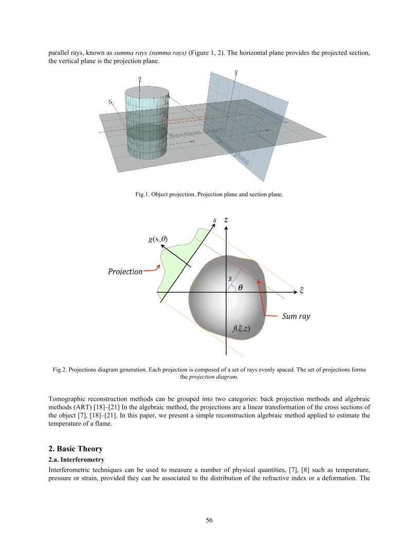
parallel rays, known as summa rays (summa rays) (Figure 1, 2). The horizontal plane provides the projected section, the vertical plane is the projection plane.

Fig.1. Object projection. Projection plane and section plane.

Fig.2. Projections diagram generation. Each projection is composed of a set of rays evenly spaced. The set of projections forms the projection diagram.

Tomographic reconstruction methods can be grouped into two categories: back projection methods and algebraic methods (ART) [18]–[21] In the algebraic method, the projections are a linear transformation of the cross sections of the object [7], [18]–[21]. In this paper, we present a simple reconstruction algebraic method applied to estimate the temperature of a flame.

2. Basic Theory 2.a. Interferometry

Interferometric techniques can be used to measure a number of physical quantities, [7], [8] such as temperature, pressure or strain, provided they can be associated to the distribution of the refractive index or a deformation. The

56

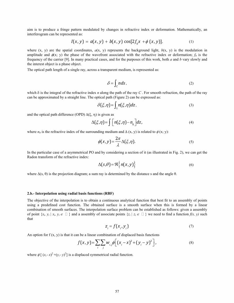
aim is to produce a fringe pattern modulated by changes in refractive index or deformation. Mathematically, an interferogram can be represented as:

I(x , y) a(x , y) b(x , y)cos[2 f0x (x , y)], (1)

where (x, y) are the spatial coordinates, a(x, y) represents the background light, b(x, y) is the modulation in amplitude and (x; y) the phase of the wavefront associated with the refractive index or deformation; f0 is the frequency of the carrier [9]. In many practical cases, and for the purposes of this work, both a and b vary slowly and the interest object is a phase object.

The optical path length of a single ray, across a transparent medium, is represented as:

ndsC , (2)

which is the integral of the refractive index n along the path of the ray C . For smooth refraction, the path of the ray can be approximated by a straight line. The optical path (Figure 2) can be expressed as:

( ,) n( ,)dzL , (3)

and the optical path difference (OPD) (, ) is given as

( ,) n( ,)n0

dz , (4)

where n0 is the refractive index of the surrounding medium and (x, y) is related to (x; y):

(x , y) 2( ,). (5)

In the particular case of a asymmetrical PO and by considering a section of it (as illustrated in Fig. 2), we can get the Radon transform of the refractive index:

(s , ) n(x , y) (6)

where Δ(s, θ) is the projection diagram; a sum ray is determined by the distance s and the angle θ.

2.b.- Interpolation using radial basis functions (RBF)

The objective of the interpolation is to obtain a continuous analytical function that best fit to an assembly of points using a predefined cost function. The obtained surface is a smooth surface when this is formed by a linear combination of smooth surfaces. The interpolation surface problem can be established as follows: given a assembly of point {xi, yi | xi, yi } and a assembly of associate points {zi | zi } we need to find a function f(x, y) such that

zi f (x

i, y

i) (7)

An option for f (x, y) is that it can be a linear combination of displaced basis functions

f (x , y) wi , j (x

i x)2 ( y

i y)2

j

i , (8)

where [ (xi - x)2 +(yi - y)2] is a displaced symmetrical radial function.

57

3. Tomographic Reconstruction In general, tomographic reconstruction process consists in obtaining an estimate of the spatial distribution of a physical quantity from its projections. The time and quality of the reconstruction depends on the reconstruction method used, the distribution of the cross section and the function associated to the reconstruction method. As shown in Fig. 2, a projection field may be expressed by

g(s , ) f (x , y) f (x , y)(xcos

ysin s)dxdy (9)

where {·} is the Radon Transform operator, f(x, y) is the distribution function and g (s, θ) represents its projections. A ray sum is given by a distance s and a slope θ.

Tomographic reconstruction problems consist of obtaining a function f̂ (x, y) from its projections g(s, θ). The estimated f̂ (x, y) may be approximated by a linear combination of basis functions. This is:

f̂ (x , y) wi , ji , j

j

i (x , y) (10)

where i,j (x, y) are general basis functions. Then, f̂ (x, y) may be expressed as:

f̂ (x , y) wi , j

i , jj

i (x , y) (11)

where Φi,j (x, y) is the radon transform of i,j (x, y).

3.a.- Proposed Method

Let f i,j a sample of , D is the interferogram wide, and θn [0, 2), then the projections diagram gm,n (sm, θn) will be given by

gm ,n(s

m,

n)

Df (x , y) f

i , j(icos

j

n jsin

n s

m)

i (12)

where D

{·} is the Discrete Radon Transform. We suppose that the sample fi,j is approximated by

fi , j w

k ,ll

k

k ,l(i , j) (13)

then the function gm,n (sm, θn) may be expressed as

gm ,n(s

m,

n) w

k ,ll

k

k ,l(s

m,

n), (14)

where wk,l are the weights, Φk,l (sm, θn) is the discrete radon transform of k,l (i, j). The vectorial form is expressed as

g =w (15)

where Φ is known as the projections matrix. Vector w minimizing

minw

g =w2s.t .(w)

i , j0 (16)

is the optimalweight vector, w*.

Let Let T : m×n → mn a transform operator, then the vectors hi,j can be defined as

58

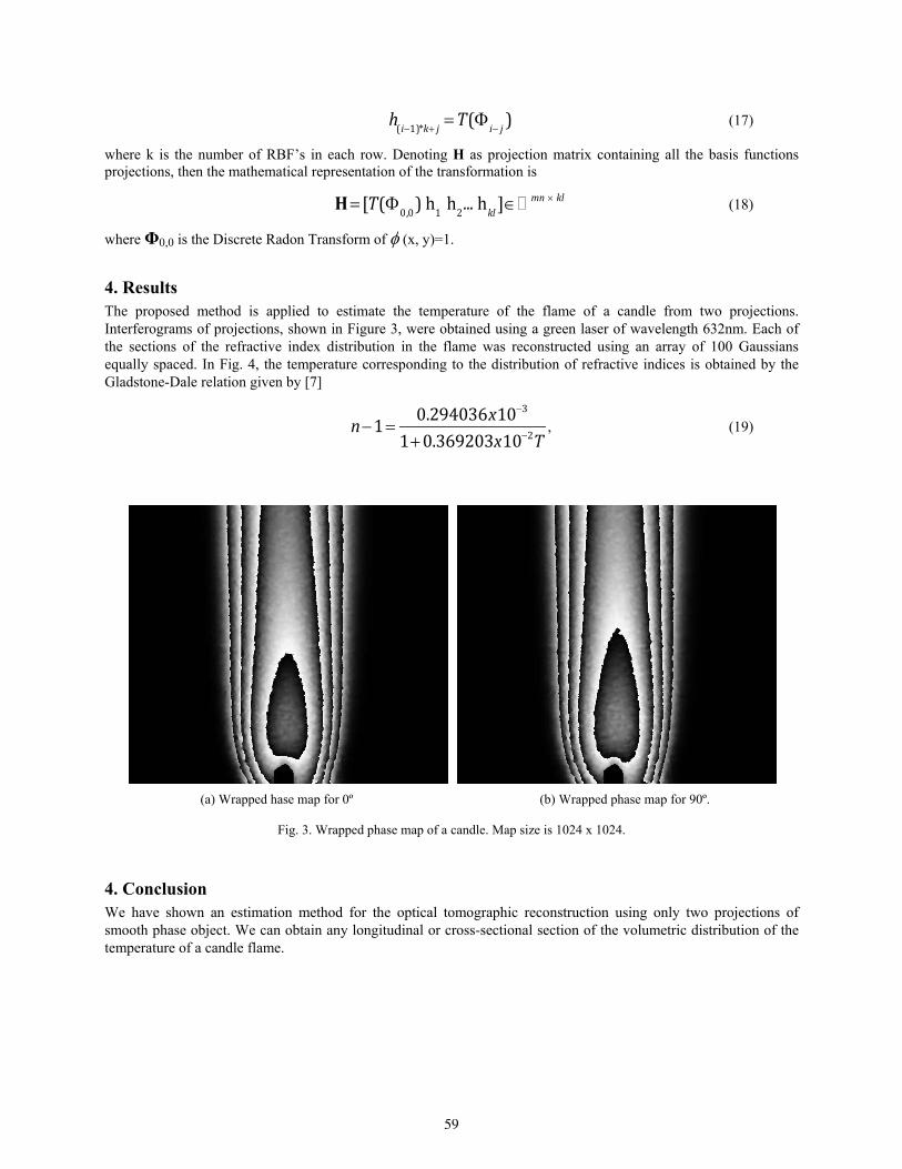
h(i1)*k j

T(i j) (17)

where k is the number of RBF’s in each row. Denoting H as projection matrix containing all the basis functions projections, then the mathematical representation of the transformation is

H [T(0,0)h

1h

2...h

kl] mn kl (18)

where Φ0,0 is the Discrete Radon Transform of (x, y)=1.

4. Results The proposed method is applied to estimate the temperature of the flame of a candle from two projections. Interferograms of projections, shown in Figure 3, were obtained using a green laser of wavelength 632nm. Each of the sections of the refractive index distribution in the flame was reconstructed using an array of 100 Gaussians equally spaced. In Fig. 4, the temperature corresponding to the distribution of refractive indices is obtained by the Gladstone-Dale relation given by [7]

n10.294036x103

10.369203x102T, (19)

(a) Wrapped hase map for 0º (b) Wrapped phase map for 90º.

Fig. 3. Wrapped phase map of a candle. Map size is 1024 x 1024.

4. Conclusion We have shown an estimation method for the optical tomographic reconstruction using only two projections of smooth phase object. We can obtain any longitudinal or cross-sectional section of the volumetric distribution of the temperature of a candle flame.

59

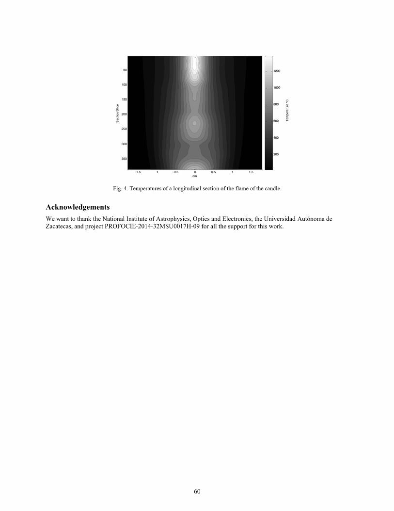
Fig. 4. Temperatures of a longitudinal section of the flame of the candle.

Acknowledgements

We want to thank the National Institute of Astrophysics, Optics and Electronics, the Universidad Autónoma de Zacatecas, and project PROFOCIE-2014-32MSU0017H-09 for all the support for this work.

60

Experimental determining the coherent-mode structure of vector electromagnetic field through its decomposition in reference basis

Esteban Vélez-Juárez, and Andrey S. Ostrovsky

Facultad de Ciencias Físico Matemáticas, Benemérita Universidad Autónoma de Puebla, Puebla 72000, México

Corresponding author email: tebanvj@hotmail.com

ABSTRACT:

A technique for experimental determining the coherent-mode structure of electromagnetic field is proposed. This technique is based on the coherence measurements of the field in some reference basis and represents a nontrivial vector generalization of the dual-mode field correlation method recently reported by F. Ferreira and M. Belsley [1]. The justifiability and efficiency of the proposed technique is illustrated by an example of determining the coherent-mode structure of some specially generated and experimentally characterized secondary electromagnetic source..

Key words: Coherence; Modes; Diffractive optics; Spatial light modulators.

REFERENCES AND LINKS [1] F. Ferreira and M. Belsley, “Holographic spatial coherence analysis of laser,” Opt. Lett. 38, 4350-4353 (2013).

[2] H. Gamo, Matrix treatment of partial coherence, in Progress in optics III, E. Wolf, ed. (North-Holland, Amsterdam, 1964) Chap. 3.

[3] E. Wolf, “New theory of partial coherence in the space-frequency domain. Part 1: Spectra and cross spectra of steady-state source,” J. Opt. Soc. Am. A, 72, 343-351 (1982).

[4] L. Mandel and E. Wolf, Optical Coherence and Quantum Optics, (Cambridge University Press, Cambridge University Press, Cambridge, UK (1995).

[5] E. Wolf, Introduction to the Coherence and Polarization of Light, (Cambridge University Press, Cambridge, UK, 2007).

[6] A. S. Ostrovsky, Coherent-Mode Representations in Optics, (SPIE Press, Bellingham, WA, 2006).

[7] F. Gori, M. Santarsiero, R. Simon, G. Piquero, R. Borghi, and G. Guattari, “Coherent-mode decomposition of partially polarized, partially coherent sources,” J. Opt. Soc. Am. A 20, 78-84 (2003).

[8] J. Tervo, T. Setälä, and A. T. Friberg, “Theory of partially coherent electromagnetic fields in the space-frequency domain,” J. Opt. Soc. Am. A 21, 2205-2215 (2004).

[9] K. Kim and E. Wolf, “A scalar-mode representation of stochastic, planar, electromagnetic sources,” Opt. Commun. 261, 19-22 (2005).

[10] F. Gori, “Matrix treatment for partially polarized partially coherent beams,” Opt. Lett. 23, 241-243 (1998).

[11] J. Tervo, T. Setälä, and A. T. Friberg, “Degree of coherence for electromagnetic fields,” Opt Express 11, 1137-1143 (2003).

[12] A. Starikov, “Effective number of degrees of freedom of partially coherent source,” J. Opt. Soc. Am. A 72, 1538-1544 (1982).

[13] A. S. Ostrovsky, G. Rodríguez-Zurita, C. Meneses-Fabián, M. Á. Olvera-Santamaría, and C. Rickenstorff-Parrao, “Experimental generating the partially coherent and partially polarized electromagnetic source,” Opt. Express 18, 12864-12871 (2010).

61

[14] C. Rickenstorff, A. S. Ostrovsky, “Measurement of the amplitude and phase modulation of a liquid crystal

spatial light modulator,” Superficies y Vacio 23(S), 36-39 (2009).

1. Introduction The coherent-mode representation of an optical field broached the first time by Gamo [2] and later on developed by Wolf [3-5] is an essential tool in describing the processes and systems in optics [6]. Not so long ago the theory of coherent-mode representation, originally developed for scalar optical fields, has been generalized to the case of vector electromagnetic fields [7-9]. This representation is defined through the solution of the Fredholm integral equation with a kernel taken as the cross-spectral density matrix of the field. However, in practice the cross-spectral density matrix of the field as a rule is unknown a priori. In theory the cross-spectral density matrix of the field can be measured with four special Young’s interference experiment [10,11], but in practice such a measurement is unfeasible in view of enormous volume of data to be processed.

Recently a new promising approach to the problem of experimental determining the coherent-mode structure of a scalar optical field has been proposed by F. Ferreira and M. Belsley [1]. This approach is based on the decomposition of a scalar field in some subsidiary orthogonal basis, which allows considerable simplification of the coherence measurements process. Here we propose the generalization of this approach to the case of a vector electromagnetic field. The justifiability and efficiency of the proposed technique is illustrated by an example of determining the coherent-mode structure of some specially generated and experimentally characterized secondary electromagnetic source.

1. Coherent-mode structure of electromagnetic field We start recalling the basic concepts of the theory of partially coherent electromagnetic fields in the space-frequency domain [8]. According to this theory the second-order statistical properties of a stochastic stationary electromagnetic field occupying some finite domain D in some plane normal to the direction of propagation and at some frequency may be completely characterized by the so-called cross-spectral density matrix (for brevity we omit the explicit dependence of the considered quantities on )

),(),(

),(),(),(

2121

212121 xxxx

xxxxxxW

yyyx

xyxx

WW

WW, (1)

where

)()(),( 2121 xxxx jiij EEW , ),,( yxji (2)

with iE and jE being the orthogonal components of the electric field vector E at two points 1x and 2x , asterisk denoting the complex conjugate, and the angle brackets denoting the average over the statistical ensemble. Furthermore, the correlation properties of a partially coherent and partially polarized electromagnetic field may be characterized quantitatively using the degree of coherence and degree of polarization defined by the formulas, respectively,

2/1

2211

2121†

21 ),(Tr),(Tr

)],(),(Tr[),(

xxWxxW

xxWxxWxx , (3)

2/1

2),(Tr

),(Det41)(

xxW

xxWxP , (4)

where Tr stands for the trace, Det denotes the determinant of matrix, and the dagger denotes the Hermitian conjunction. As has been shown in Ref. 8, under very general conditions the cross-spectral density matrix W may be represented in the form of series, i.e.,

),(),( 2121 xxWxxW nn

n ,...)2,1,0( n , (5)

where ),( 21 xxWn is the 22 matrix with elements

62

)()(),( 2;1;21; xxxx njninijW . (6)

In Eq. (5) n and )()( xin are the eigenvalues and the eigenfunctions of two coupled integral equations

)(d)(),( 2;11;21; xxxxx ninj

DnjnijW . (7)

The eigenvalues are real and nonnegative, and the eigenfunctions satisfy the orthonormality condition

nmD

mini xxx d)()( ;; , (8)

where nm is the Kronecker symbol. Each matrix ),( 21 xxWn in Eq. (5) can be associated with an elementary mode of the field which is completely coherent ( 1n ) and completely polarized ( 1nP ).Therefore the set of n and )(; xni is referred to as the coherent-mode structure of the field. It must be noted that in practice one needs truncating the coherent-mode structure by finite number N of terms, which depends on the degree of coherence of the field [12]. 2. Decomposition of the coherent-mode structure in reference basis Now, adopting the main idea of Ref. 1 originally formulated for a scalar field, we will show that the coherent-mode structure of a vector electromagnetic field may be defined in a more practical way. To do this, we assume that the realizations of each orthogonal component iE of the electric field vector can be expanded in some orthogonal basis )}({ xk , which we will refer to the reference basis, as follows:

k

kkii aE )()( ; xx , (9)

klD

lk xxx d)()( , (10)

xxx d)()(; D

kiki Ea . (11)

Substituting for iE from Eq. (9) into Eq. (2), we obtain

k l

lkklijij cW )()(),( 21;21 xxxx , (12)

where

ljkiklij aac ;;; . (13)

Substituting from Eq. (12) into Eq. (7), we find

)()( ;;;; xx ninj

lk l

knjklij bc , (14)

where

D

knjknjb xxx d)()(;;; , (15)

Finally, multiplying both sides of Eq. (14) by )(xs and integrating the result over x with due regard for the orthogonality

relation (10), we obtain the system of algebraic equations

lninj k

knjklij bbc ;;;;; . (16)

This system can be written in matrix form as follows:

ny

nxn

ny

nx

yyxy

xyxx

;

;

;

;†

B

B

B

B

CC

CC , (17)

63

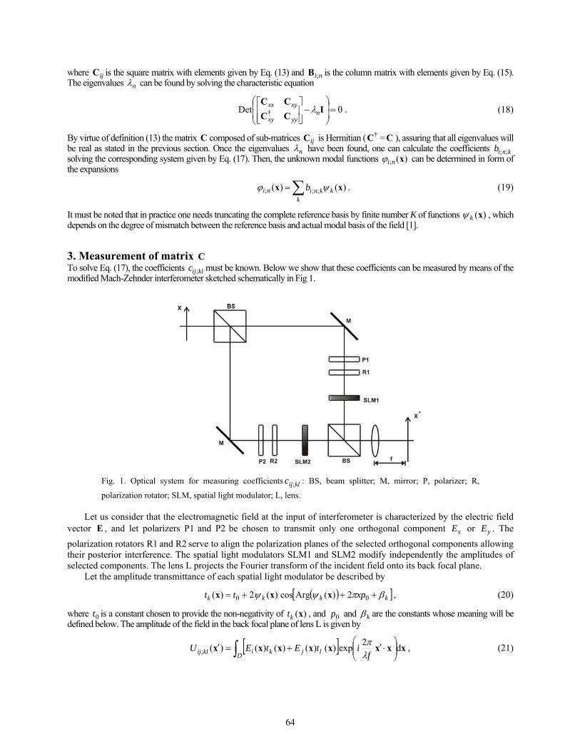
where ijC is the square matrix with elements given by Eq. (13) and ni;B is the column matrix with elements given by Eq. (15). The eigenvalues n can be found by solving the characteristic equation

0Det †

I

CC

CCn

yyxy

xyxx . (18)

By virtue of definition (13) the matrix C composed of sub-matrices ijC is Hermitian ( †C =C ), assuring that all eigenvalues will be real as stated in the previous section. Once the eigenvalues n have been found, one can calculate the coefficients knib ;; solving the corresponding system given by Eq. (17). Then, the unknown modal functions )(; xni can be determined in form of the expansions

k

kknini b )()( ;;; xx . (19)

It must be noted that in practice one needs truncating the complete reference basis by finite number K of functions )(xk , which depends on the degree of mismatch between the reference basis and actual modal basis of the field [1].

3. Measurement of matrix C To solve Eq. (17), the coefficients klijc ; must be known. Below we show that these coefficients can be measured by means of the modified Mach-Zehnder interferometer sketched schematically in Fig 1.

Fig. 1. Optical system for measuring coefficients klijc ; : BS, beam splitter; M, mirror; P, polarizer; R,

polarization rotator; SLM, spatial light modulator; L, lens. Let us consider that the electromagnetic field at the input of interferometer is characterized by the electric field

vector E , and let polarizers P1 and P2 be chosen to transmit only one orthogonal component xE or yE . The

polarization rotators R1 and R2 serve to align the polarization planes of the selected orthogonal components allowing their posterior interference. The spatial light modulators SLM1 and SLM2 modify independently the amplitudes of selected components. The lens L projects the Fourier transform of the incident field onto its back focal plane.

Let the amplitude transmittance of each spatial light modulator be described by

kkkk xptt 00 2)(Argcos)(2)( xxx , (20)

where 0t is a constant chosen to provide the non-negativity of )(xkt , and 0p and k are the constants whose meaning will be defined below. The amplitude of the field in the back focal plane of lens L is given by

Dljkiklij f

itEtEU xxxxxxxx d2

exp)()()()()(;

, (21)

64

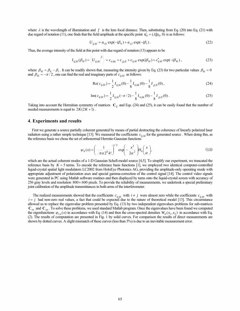
where is the wavelength of illumination and f is the lens focal distance. Then, substituting from Eq. (20) into Eq. (21) with due regard of notation (11), one finds that the field amplitude at the specific point )0 ,( 00 fpx is as follows:

)exp()exp( ;;; lljkkiklij iaiaU . (22)

Thus, the average intensity of the field at this point with due regard of notation (13) appears to be

2

;; )( klijklklij UI )exp()exp( ;;;; klklijklklijlljjkkii iciccc , (23)

where lkkl . It can be readily shown that, measuring the intensity given by Eq. (23) for two particular values 0kl and 2/ kl , one can find the real and imaginary parts of klijc ; as follows:

)0(8

1)0(

8

1)0(

2

1) Re( ;;;; lljjkkiiklijklij IIIc , (24)

)0(8

1)0(

8

1)2/(

2

1) Im( ;;;; lljjkkiiklijklij IIIc . (25)

Taking into account the Hermitian symmetry of matrices ijC and Eqs. (24) and (25), it can be easily found that the number of needed measurements is equal to )12(2 KK .

4. Experiments and results First we generate a source partially coherent generated by means of partial destructing the coherence of linearly polarized laser radiation using a rather simple technique [13]. We measured the coefficients klijc ; for the generated source . When doing this, as the reference basis we chose the set of orthonormal Hermite-Gaussian functions

x

Hx

kx kkk 2

22/1

2exp

!2

1)( , (15)

which are the actual coherent modes of a 1-D Gaussian Schell-model source [4,5]. To simplify our experiment, we truncated the reference basis by 5K terms. To encode the reference basis functions [1], we employed two identical computer-controlled liquid-crystal spatial light modulators LC2002 from HoloEye Photonics AG, providing the amplitude-only operating mode with appropriate adjustment of polarization axes and special gamma-correction of the control signal [14]. The control video signals were generated in PC using Matlab software routines and then displayed by turns onto the liquid-crystal screen with accuracy of 256 gray levels and resolution 600800 pixels. To provide the reliability of measurements, we undertook a special preliminary joint calibration of the amplitude transmittances in both arms of the interferometer. The realized measurements showed that the coefficients klijc ; with ji were almost zero while the coefficients klijc ; with

ji had non-zero real values, a fact that could be expected due to the nature of theoretical model [13]. This circumstance allowed us to replace the eigenvalue problem presented by Eq. (13) by two independent eigenvalues problems for sub-matrices

xxC and yyC . To solve these problems, we used standard Matlab program. Once the eigenvalues have been found we computed the eigenfunctions )(; xni in accordance with Eq. (14) and then the cross-spectral densities ),( 21 xxWii in accordance with Eq. (2). The results of computation are presented in Fig. 1 by solid curves. For comparison the results of direct measurements are shown by dotted curves. A slight mismatch of these curves (less than 5%) is due to an inevitable measurement error.

65

Fig. 1. Normalized cross-spectral densities of generated secondary source measured in experiment (dotted curves) and determined in accordance with the proposed technique (solid curves) for ground glass plates with diffusion angles of 10◦ (a) and 30◦ (b).

5. Conclusions We have proposed a technique of experimental determining the coherent-mode structure of electromagnetic field. This technique is based on the coherence measurements of the field in some reference basis and represents a nontrivial vector generalization of the dual-mode field correlation method recently reported by F. Ferreira and M. Belsley for a scalar case [1]. The justifiability and efficiency of the proposed technique has been demonstrated with an example of determining the coherent-mode structure of some specially generated and experimentally characterized secondary electromagnetic source.

Acknowledgements

This work was supported by the Benemérita Universidad Autónoma de Puebla (project VIEP OSA-EXC-14) and by the National Council for Science and Technology of Mexico (project CB-165142).

66

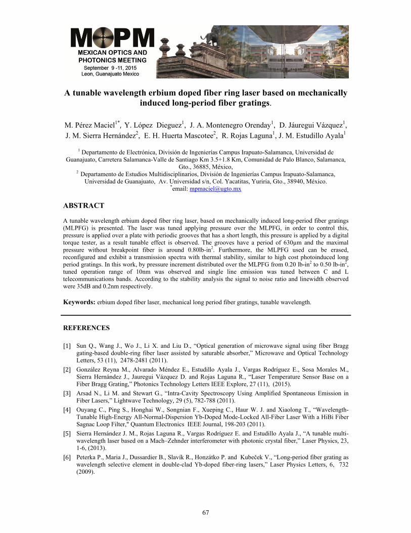
A tunable wavelength erbium doped fiber ring laser based on mechanically

induced long-period fiber gratings.

M. Pérez Maciel1*, Y. López Dieguez1, J. A. Montenegro Orenday1, D. Jáuregui Vázquez1, J. M. Sierra Hernández2, E. H. Huerta Mascotee2, R. Rojas Laguna1, J. M. Estudillo Ayala1

1 Departamento de Electrónica, División de Ingenierías Campus Irapuato-Salamanca, Universidad de

Guanajuato, Carretera Salamanca-Valle de Santiago Km 3.5+1.8 Km, Comunidad de Palo Blanco, Salamanca, Gto., 36885, México,

2 Departamento de Estudios Multidisciplinarios, División de Ingenierías Campus Irapuato-Salamanca, Universidad de Guanajuato, Av. Universidad s/n, Col. Yacatitas, Yuriria, Gto., 38940, México.

*email: mpmaciel@ugto.mx ABSTRACT A tunable wavelength erbium doped fiber ring laser, based on mechanically induced long-period fiber gratings (MLPFG) is presented. The laser was tuned applying pressure over the MLPFG, in order to control this, pressure is applied over a plate with periodic grooves that has a short length, this pressure is applied by a digital torque tester, as a result tunable effect is observed. The grooves have a period of 630µm and the maximal pressure without breakpoint fiber is around 0.80lb-in2. Furthermore, the MLPFG used can be erased, reconfigured and exhibit a transmission spectra with thermal stability, similar to high cost photoinduced long period gratings. In this work, by pressure increment distributed over the MLPFG from 0.20 lb-in2 to 0.50 lb-in2, tuned operation range of 10nm was observed and single line emission was tuned between C and L telecommunications bands. According to the stability analysis the signal to noise ratio and linewidth observed were 35dB and 0.2nm respectively. Keywords: erbium doped fiber laser, mechanical long period fiber gratings, tunable wavelength. REFERENCES [1] Sun Q., Wang J., Wo J., Li X. and Liu D., “Optical generation of microwave signal using fiber Bragg

gating-based double-ring fiber laser assisted by saturable absorber,” Microwave and Optical Technology Letters, 53 (11), 2478-2481 (2011).

[2] González Reyna M., Alvarado Méndez E., Estudillo Ayala J., Vargas Rodríguez E., Sosa Morales M., Sierra Hernández J., Jauregui Vázquez D. and Rojas Laguna R., “Laser Temperature Sensor Base on a Fiber Bragg Grating,” Photonics Technology Letters IEEE Explore, 27 (11), (2015).

[3] Arsad N., Li M. and Stewart G., “Intra-Cavity Spectroscopy Using Amplified Spontaneous Emission in Fiber Lasers,” Lightwave Technology, 29 (5), 782-788 (2011).

[4] Ouyang C., Ping S., Honghai W., Songnian F., Xueping C., Haur W. J. and Xiaolong T., “Wavelength-Tunable High-Energy All-Normal-Dispersion Yb-Doped Mode-Locked All-Fiber Laser With a HiBi Fiber Sagnac Loop Filter," Quantum Electronics IEEE Journal, 198-203 (2011).

[5] Sierra Hernández J. M., Rojas Laguna R., Vargas Rodríguez E. and Estudillo Ayala J., “A tunable multi-wavelength laser based on a Mach–Zehnder interferometer with photonic crystal fiber,” Laser Physics, 23,1-6, (2013).

[6] Peterka P., Maria J., Dussardier B., Slavík R., Honzátko P. and Kubeček V., “Long-period fiber grating as wavelength selective element in double-clad Yb-doped fiber-ring lasers,” Laser Physics Letters, 6, 732 (2009).

67

[7] Fallnich C. and Walbaum T., “Wavelength tuning of multimode interference bandpass filters by mechanical bending: experiment and theory in comparison,” Appl. Phys., 108, 117-124 (2012).

[8] González García A., Pottiez O. and Grajales Coutiño R., “Estudio experimental de un láser sintonizable en longitud de onda usando un filtro de Sagnac con selectividad espectral mediante cambios en la temperatura,” Revista Mexicana de Fisica, 56( 4), 275-280 (2010).

[9] Xiufeng Y., Xinyong D., Shumin Z., Lu F., Xiaoqun Z. and Chao L., “Multiwavelength erbium-doped fiber laser with 0.8-nm spacing using sampled Bragg grating and photonic crystal fiber,” Photonics Technology Letters IEEE, 17, 2538-2540 (2005).

[10]Causado Buelvas J. D., Gómez Cardona N. D., Torres P. and Gómez J. A., “Láser Sintonizable en Anillo de Fibra Dopada con Erbio,” Revista Colombiana de Fisica, 7 (1), 1-7 (2009).

[11]Budynas R. G., Shigley J. E. and Nisbett J. K., [Mechanical Engineering Design], McGraw-Hill, (2007).

[12]Huerta-Mascotte E., Estudillo-Ayala J. M., Mata-Chávez R. I., Guzmán-Chávez A. D., Jauregui-VázquezD., Sierra-Hernández J. M., Hernández-Garcia J. C., Vargas-Rodríguez E. and Rojas-Laguna R., “Characterization of long-period fiber grating as load sensing,” Proc. SPIE 92001D-2, (2014).

[13]Sakata H., Yoshimi H. and Otake Y., “Wavelength tunability of L-band fiber ring lasers using mechanically induced long-period fiber gratings,” Optics Communications, 282, 1179–1182 (2009).

1. INTRODUCTION

Several Erbium Doped Fiber Lasers (EDFL) haven been studied due to their multiples applications such as: optical communications systems [1], fiber optic sensing devices [2], optical signal analysis and spectroscopy [3]. These lasers offer flexibility, compactness and good gain power output. Most of the lasers exposed deals with the mode competition [4], this effect generated wavelengths emissions, instable lasing and limited switch combinations. As a result many tunable technique have been demonstrated: Mach-Zehnder interferometer [5], fiber Bragg grating [6], multimode fiber structures [7], Sagnac interferometer [8], special photonic crystal fibers [9] and Fabry-Perot filters [10]. One of the most attractive techniques to tune a fiber laser is based on mechanical long period fiber gratings (MLPFG) due to its low cost, works as a temporary filter, and several sensitivity parameters (pressure, tension, twist angle and period) that generated change losses into the filter spectrum, these losses variations generated a wavelength dependence at specific lasing modes into a fiber laser cavity. In this work we present a tunable single line ring fiber laser, here the single lasing wavelength is centered at 1570.42nm and it was tuned by losses modification generated when the pressure applied over the MLPFG is changed. The operation range observed in the laser-tuned spectrum was from 1560nm to 1570nm, moreover the minimal mode spacing that can be obtained by pressuring the MLPFG is around 0.1nm.

2. EXPERIMENTAL SETUP

The schematic configuration of the single ring fiber laser is showed at Fig.1. The main components of the laser are: the pumped diode (QFBGLD-980-200) with a maximal power of 208 mW, the gain medium in this case an Erbium Doped Fiber (EDF) with a length of 3.5m (Erbium Doped Fiber-LIEKKI™ Er 16-8/125) and the fiber filter (MLPFG). Here, the pumped light was coupled to the ring cavity by a 980/1550nm optical fiber wavelength division multiplexer (WDM) and directed to the EDF. Once the light pass through the EDF, the signal is propagated to the optical fiber coupler 90%/10%, here the 90% of the signal will remains re-circulating into the cavity to ensure the amplification spontaneous emission (ASE) which will conserve the high gain medium, by using 10% port coupler the output fiber laser is monitoring by an Optical Spectrum Analyzer (OSA) Yokogawa, AQ6370. Moreover, by a polarization controller (PC), the polarization stage is set into the ring cavity with the purpose to stabilize the power output fiber laser. Besides, an optical fiber isolator was used to provide unidirectional light propagation into the ring cavity.

68

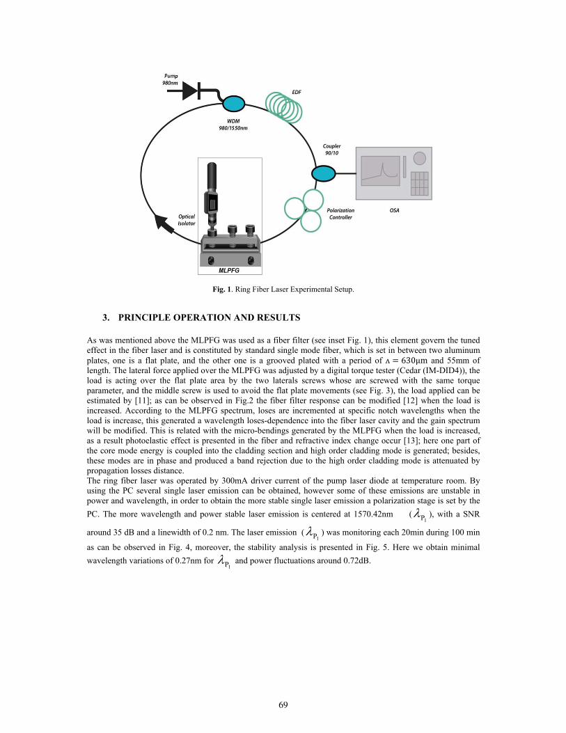
Fig. 1. Ring Fiber Laser Experimental Setup.

3. PRINCIPLE OPERATION AND RESULTS

As was mentioned above the MLPFG was used as a fiber filter (see inset Fig. 1), this element govern the tuned effect in the fiber laser and is constituted by standard single mode fiber, which is set in between two aluminum plates, one is a flat plate, and the other one is a grooved plated with a period of ʌ 630μm and 55mm of length. The lateral force applied over the MLPFG was adjusted by a digital torque tester (Cedar (IM-DID4)), the load is acting over the flat plate area by the two laterals screws whose are screwed with the same torque parameter, and the middle screw is used to avoid the flat plate movements (see Fig. 3), the load applied can be estimated by [11]; as can be observed in Fig.2 the fiber filter response can be modified [12] when the load is increased. According to the MLPFG spectrum, loses are incremented at specific notch wavelengths when the load is increase, this generated a wavelength loses-dependence into the fiber laser cavity and the gain spectrum will be modified. This is related with the micro-bendings generated by the MLPFG when the load is increased, as a result photoelastic effect is presented in the fiber and refractive index change occur [13]; here one part of the core mode energy is coupled into the cladding section and high order cladding mode is generated; besides, these modes are in phase and produced a band rejection due to the high order cladding mode is attenuated by propagation losses distance. The ring fiber laser was operated by 300mA driver current of the pump laser diode at temperature room. By using the PC several single laser emission can be obtained, however some of these emissions are unstable in power and wavelength, in order to obtain the more stable single laser emission a polarization stage is set by the

PC. The more wavelength and power stable laser emission is centered at 1570.42nm ( ), with a SNR

around 35 dB and a linewidth of 0.2 nm. The laser emission ( ) was monitoring each 20min during 100 min

as can be observed in Fig. 4, moreover, the stability analysis is presented in Fig. 5. Here we obtain minimal

wavelength variations of 0.27nm for and power fluctuations around 0.72dB.

P1

P1

P1

69

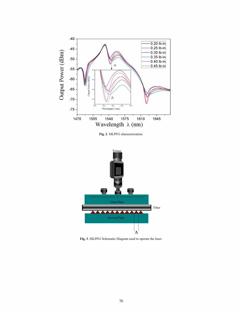
Fig. 2. MLPFG characterization.

Fig. 3. MLPFG Schematic Diagram used to operate the laser.

70

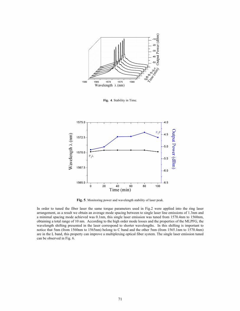
Fig. 4. Stability in Time.

Fig. 5. Monitoring power and wavelength stability of laser peak. In order to tuned the fiber laser the same torque parameters used in Fig.2 were applied into the ring laser arrangement, as a result we obtain an average mode spacing between to single laser line emissions of 1.3nm and a minimal spacing mode achieved was 0.1nm, this single laser emission was tuned from 1570.4nm to 1560nm, obtaining a total range of 10 nm. According to the high order mode losses and the properties of the MLPFG, the wavelength shifting presented in the laser correspond to shorter wavelengths. In this shifting is important to notice that 5nm (from 1560nm to 1565nm) belong to C band and the other 5nm (from 1565.1nm to 1570.4nm) are in the L band, this property can improve a multiplexing optical fiber system. The single laser emission tuned can be observed in Fig. 6.

71

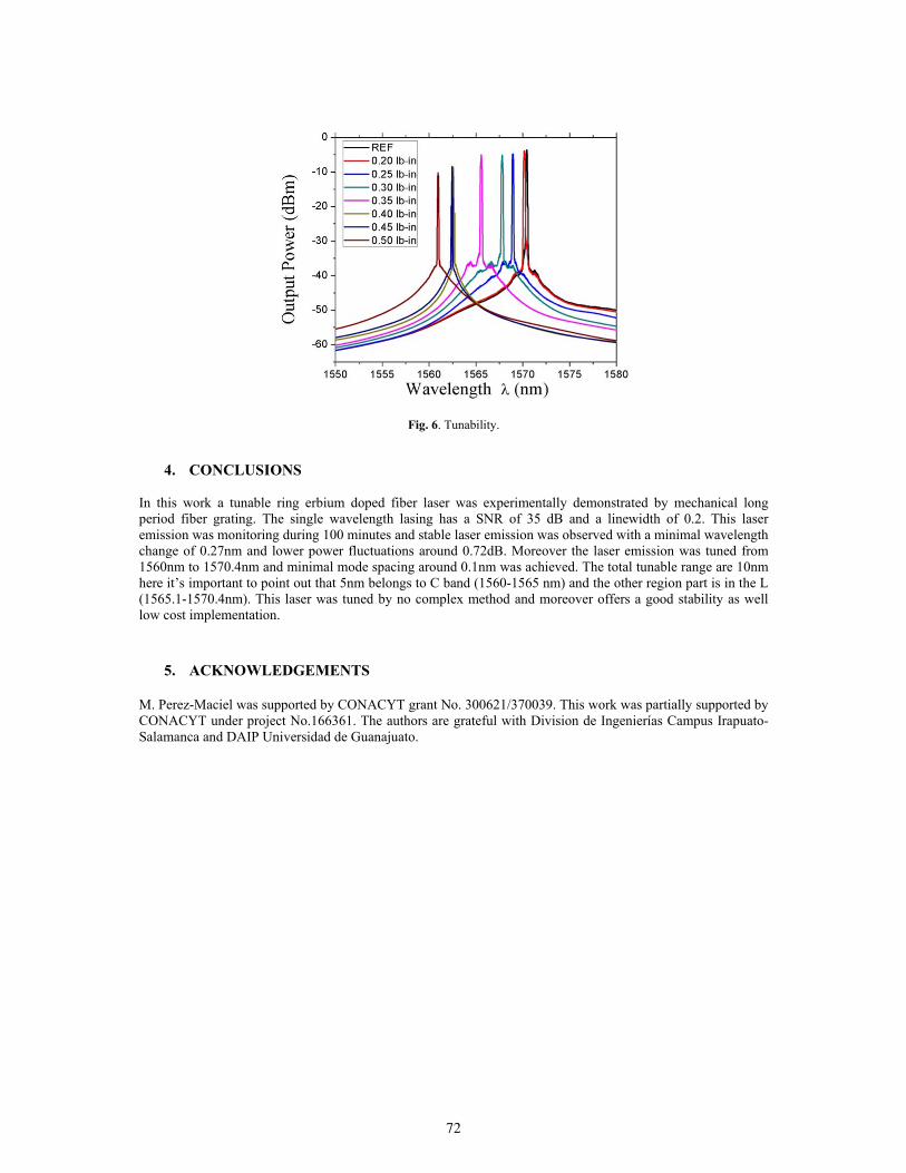
Fig. 6. Tunability.

4. CONCLUSIONS

In this work a tunable ring erbium doped fiber laser was experimentally demonstrated by mechanical long period fiber grating. The single wavelength lasing has a SNR of 35 dB and a linewidth of 0.2. This laser emission was monitoring during 100 minutes and stable laser emission was observed with a minimal wavelength change of 0.27nm and lower power fluctuations around 0.72dB. Moreover the laser emission was tuned from 1560nm to 1570.4nm and minimal mode spacing around 0.1nm was achieved. The total tunable range are 10nm here it’s important to point out that 5nm belongs to C band (1560-1565 nm) and the other region part is in the L (1565.1-1570.4nm). This laser was tuned by no complex method and moreover offers a good stability as well low cost implementation.

5. ACKNOWLEDGEMENTS

M. Perez-Maciel was supported by CONACYT grant No. 300621/370039. This work was partially supported by CONACYT under project No.166361. The authors are grateful with Division de Ingenierías Campus Irapuato-Salamanca and DAIP Universidad de Guanajuato.

72

Line Emission Identification of LIBS Generated Plasmas of Unknown Samples

I. Rosas-Román, M.A. Meneses-Nava(1),O. Barbosa-García, J.L. Maldonado, G. Ramos-Ortiz

Centro de Investigaciones en Óptica, León, Gto., México

(1)Corresponding author email: tono@cio.mx

ABSTRACT:

Laser–Induced Breakdown Spectroscopy (LIBS) is a technique that allows to identify elemental composition of samples. LIBS has many advantages like, speed in spectral acquisition, works on solids, liquids and gases, samples do not need previous preparation, among others. Basically, it consists in focusing a pulsed laser beam on a sample surface, producing plasma, whose light is analyzed in a dispersive instrument. The resulting spectra are composed of narrow bands that are characteristic for each atomic species in the sample. Line identification in LIBS spectra it is not a trivial task, because it is usually composed of tens of lines in spectral ranges as narrow as 20–30 nm, and the intensity of the emission is affected by the matrix effect. Moreover the emission of some different atomic species share lines separated by a few hundredths of a nanometer. This work proposes a method that can be used as an auxiliary tool for elemental identification in LIBS produced plasmas. Basically, generates a coefficient that indicates the matching strength of an element in the spectrum. The elements with higher coefficients are then used to produce a synthetic spectrum which in turns is compared with the experimental data in order to get a match decision.

Key words: Elemental Identification, Band Searching, LIBS

REFERENCES AND LINKS

[1] A. Ciucci, M. Corsi, V. Palleschi, S. Rastelli, A. Salvetti, and E. Tognoni, New Procedure for Quantitative Elemental Analysis by Laser-Induced Plasma Spectroscopy, Applied Spectroscopy, (53) 960-964, 1999

[2] P. Griffiths and L. Shao, Self-Weighted Correlation Coefficients and Their Application to Measure Spectral Similarity, Applied Spectroscopy, (63) 916-919, 2009

[3] Kramida, A., Ralchenko, Yu., Reader, J. and NIST ASD Team (2014). NIST Atomic Spectra Database (version 5.2), [Online]. Available: http://physics.nist.gov/asd. National Institute of Standards and Technology, Gaithersburg, MD.

1. Introduction Laser Induced Breakdown Spectroscopy (LIBS) is a technique that analyses plasma light emission produced by focusing a pulsed laser on a sample surface. Emission bands in a spectrum are unique fingerprints for every atomic element in the sample and can be employed to determinate the elemental composition.

Automatic line identification has remained as an open problem because there is not a satisfactory correlation method that can be compared with the human ability to discriminate similar shapes. Besides a huge number of reference lines, the emission of some different atomic species share lines separated by a few hundredths of nanometer, increasing the complexity of the searching methods.

73

This work proposes a semi-automated approach for elemental identification in LIBS produced plasmas, based by two stage strategy. The first step reduces the possible matching species by wavelength band position, while the second step makes a weighted correlation with synthetically generated spectra.

2. Theoretical Model As stated earlier, a synthetic spectrum is needed for amplitude comparison, which is based on a procedure proposed in 1999 [1] aimed to get quantitative composition from LIBS spectra. It’s based on the following plasma properties assumptions: a) Is stoichiometric, b) Is in Local Thermal Equilibrium (LTE), c) The radiation source is optically thin. Under this hypothesis, the line integral intensity corresponding to the transition from energetic states Ei to Ek is:

/

( )

k BE Tkki ki k

ss

A g eI FC

U T

(1)

where Aki is the transition probability for the given line, gk is the level degeneracy, Us(T) is the partition function for the emitting species in the plasma, kB is the Boltzmann constant, T is the plasma temperature, Cs represents the concentration of the emitting species and F is an experimental parameter that takes into account the plasma density and volume as well as the optical efficiency of the collection system.

Assuming self-absorption as negligible, a synthetic spectrum can be calculated—proposing a plasma temperature and a scale factor—as a superposition of Lorentzian shape bands. The central position can be obtained at NIST database, amplitude is calculated from equation 1, and FWHM can be estimated by the minimum line width resolution of the spectrometer used.

The scaling factor F Cs relationship was calculated in the same way as Griffiths [2] who proposes equation 2 to eliminate signal strength differences in a weighted correlation procedure.

t

t

r sk

r r

(2)

2. Procedure Experimental bands are compared against Atomic Spectra Database at NIST [3] available at the web. Since atomic species information is embedded on a web page, a PYTHON program was written to extract it as an ASCII file, which in turns is processed by C++ program in order to get a MATLAB file format. This process was applied in a range from 200 to 900 nm for every atomic species.

LIB plasma was generated from a copper ore sample with a picosecond pulsed Nd:Yag laser at 532 nm and 30 J of energy. Plasma emission was detected with a 500 mm focal length Czerny-Turner spectrometer and an intensified CCD camera. Several windows had to be taken in order to cover a 250-900 nm spectral range.

The first step on identification is to compare the central wavelength of each spectral band against the NIST species database. Central wavelength in the measured spectra can be estimated by the first derivative criterion. Should be pointed out that experimental data must be wavelength calibrated, baseline corrected and normalized before peak detection. A significant time saving strategy is to compare only elements with higher emission in every window.

This work proposes a binary numerical match factor w, calculated according to the following relationship:

( )

1

2n

z i

i

w

(3)

where z is a binary vector sorted in descending order according to its intensities as reported at NIST. A minimum acceptance threshold is set to w, thus reducing the possible matching species.

74

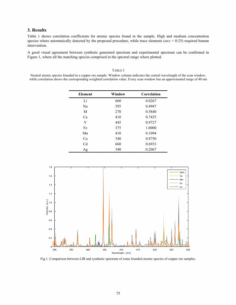
3. Results Table 1 shows correlation coefficients for atomic species found in the sample. High and medium concentration species where automatically detected by the proposed procedure, while trace elements (wcc < 0:25) required human intervention.

A good visual agreement between synthetic generated spectrum and experimental spectrum can be confirmed in Figure 1, where all the matching species comprised in the spectral range where plotted.

TABLE I

Neutral atomic species founded in a copper ore sample. Window column indicates the central wavelength of the scan window, while correlation shows the corresponding weighted correlation value. Every scan window has an approximated range of 40 nm

Element Window Correlation

Li 660 0.0267

Na 595 0.4947

M 270 0.5840

Ca 410 0.7425

V 445 0.9727

Fe 375 1.0000

Mn 410 0.1094

Cu 340 0.8750

Cd 660 0.6933

Ag 340 0.2067

Fig.1. Comparison between LIB and synthetic spectrum of some founded atomic species of copper ore samples.

75

4. Conclusions The proposed procedure is suitable for the automatic identification of high concentration species of ores samples. Medium concentration elements were also found and their presence was suggested by the composition of other ores employed elsewhere.

Trace element identification is still a challenge and requires human intervention, but this limitation is shared among other common analytic techniques which are time consuming and requires laborious sample preparation.

76

Design and construction of optical waveguides through femtosecond laser micromachining

H. E. Lazcano, R. A. Torres, G. V. Vázquez.

Centro de Investigaciones en Óptica, Loma del Bosque 115, Lomas del Campestre, C.P. 37150, León, Gto.

México. hugoelh@cio.mx

ABSTRACT:

In this work, surface waveguides were fabricated using an ultrafast Libra Coherent laser with a central wavelength at 800 nm, a repetition rate of 1 kHz and pulse duration of about 50 fs, as well as a Laser Microfabrication Workstation (mFAB Newport). The waveguides were written along the width of glass slides (Corning 2947B), with writing speeds ranging from 50 to 1000 μm/s. The waveguides have widths ranging from 8 to 20 μm, depending on the translation speed, focus and acceleration settings. The profile of the grooves has a triangular shape. In order to guarantee no interaction between waveguides, we spaced them by more than 15 μm from each other. To accomplish the analysis, the input and output surfaces of the waveguides were polished. The near field was observed using a CCD camera beam profiler (Thorlabs BC106-VIS). Preliminarily, the average transmission loss of the fabricated straight waveguides is about 6.5 dB/cm at 633nm. Outcomes of this study are promising for use in the manufacturing of sensing devices.

Keywords: optical waveguides, laser micromachining.

REFERENCES AND LINKS

[1] K. M. Davis, K. Miura, N. Sugimoto, and K. Hirao, “Writing waveguides in glass with a femtosecond laser”, Optics Letters, Vol. 21, No. 21, 1729-1731 (1996).

[2] R. R. Gattass, L. R. Cerami and E. Mazur, “Micromachining of bulk glass with bursts of femtosecond laser pulses at variable repetition rates”, Optics Express, Vol. 14, No. 12, 5279- 5284 (2006).

[3] Ch. B. Schaffer, A. Brodeur, J. F. García, and E. Mazur, “Micromachining bulk glass by use of femtosecond laser pulses with nanojoule energy”, Optics Letters, Vol. 26, No. 2 93-95, (2001).

[4] L. Tong, R. R. Gattass, I. Maxwell, J. B. Ashcom and E. Mazur “Optical loss measurements in femtosecond laser written waveguides in glass”, Optics Communications 259, 626–630 (2006)

[5] R. R. Gattass, Femtosecond-laser interactions with transparent materials: applications in micromachining and supercontinuum generation, Harvard University Cambridge, Massachusetts (2006).

[6] M. R. Tijerina. Caracterización de guías de onda ópticas generadas con láser de femtosegundos en Niobato de Litio. Universidad Nacional de La Plata, La Plata, Argentina (2014)

[7] H. Lazcano,J. L. Flores, A. Blanco, A. Hernández, R. Nieto, J. L. Martínez, R. A. Torres, G. V. Vázquez, J. L. Hurtado, “High quality polishing procedure of glass substrates: application in integrated optics”. ISEM SOI 2015, Conference Proceedings of the Society for Experimental Mechanics Series, Springer International Publishing AG.

[8] J. F. Bourhis, “Fibre to waveguide connection”, in “Glass Integrated Optics and Optical Fiber Devices”, Critical Reviews of Optical Science and Technology, SPIE Optical Engineering Press, Vol.CR53, 335-366, (1994).

77

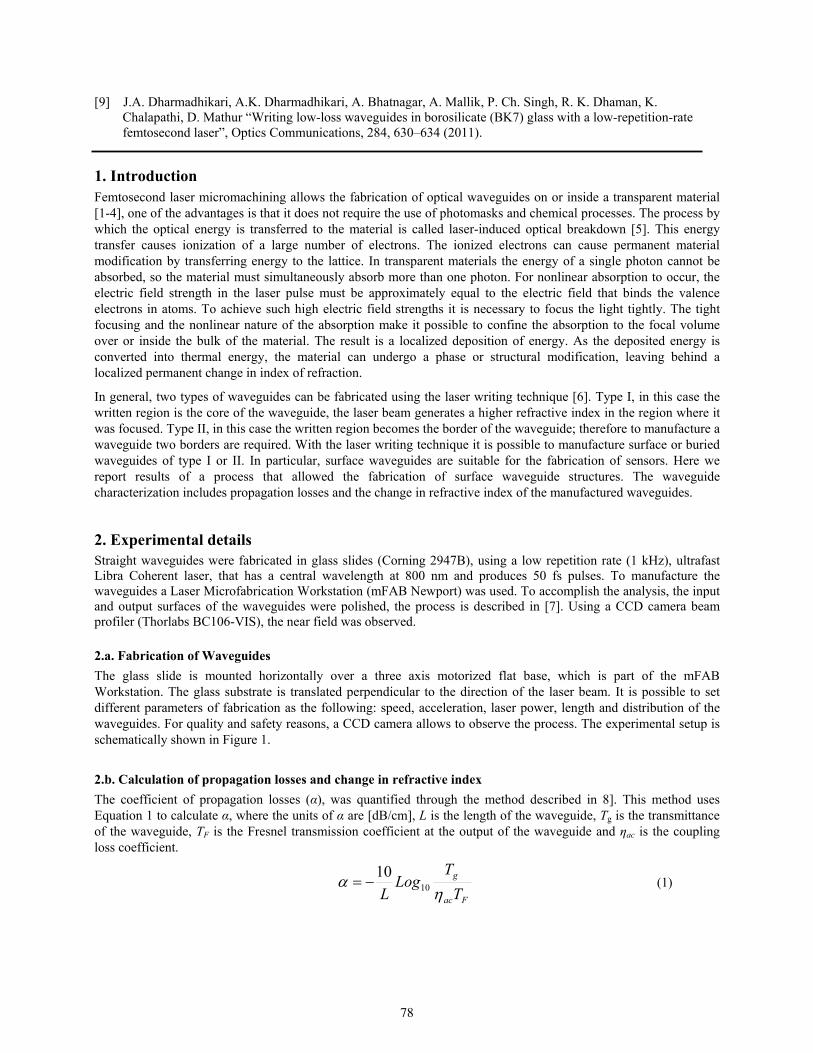
[9] J.A. Dharmadhikari, A.K. Dharmadhikari, A. Bhatnagar, A. Mallik, P. Ch. Singh, R. K. Dhaman, K.

Chalapathi, D. Mathur “Writing low-loss waveguides in borosilicate (BK7) glass with a low-repetition-rate femtosecond laser”, Optics Communications, 284, 630–634 (2011).

1. Introduction Femtosecond laser micromachining allows the fabrication of optical waveguides on or inside a transparent material [1-4], one of the advantages is that it does not require the use of photomasks and chemical processes. The process by which the optical energy is transferred to the material is called laser-induced optical breakdown [5]. This energy transfer causes ionization of a large number of electrons. The ionized electrons can cause permanent material modification by transferring energy to the lattice. In transparent materials the energy of a single photon cannot be absorbed, so the material must simultaneously absorb more than one photon. For nonlinear absorption to occur, the electric field strength in the laser pulse must be approximately equal to the electric field that binds the valence electrons in atoms. To achieve such high electric field strengths it is necessary to focus the light tightly. The tight focusing and the nonlinear nature of the absorption make it possible to confine the absorption to the focal volume over or inside the bulk of the material. The result is a localized deposition of energy. As the deposited energy is converted into thermal energy, the material can undergo a phase or structural modification, leaving behind a localized permanent change in index of refraction.

In general, two types of waveguides can be fabricated using the laser writing technique [6]. Type I, in this case the written region is the core of the waveguide, the laser beam generates a higher refractive index in the region where it was focused. Type II, in this case the written region becomes the border of the waveguide; therefore to manufacture a waveguide two borders are required. With the laser writing technique it is possible to manufacture surface or buried waveguides of type I or II. In particular, surface waveguides are suitable for the fabrication of sensors. Here we report results of a process that allowed the fabrication of surface waveguide structures. The waveguide characterization includes propagation losses and the change in refractive index of the manufactured waveguides.

2. Experimental details Straight waveguides were fabricated in glass slides (Corning 2947B), using a low repetition rate (1 kHz), ultrafast Libra Coherent laser, that has a central wavelength at 800 nm and produces 50 fs pulses. To manufacture the waveguides a Laser Microfabrication Workstation (mFAB Newport) was used. To accomplish the analysis, the input and output surfaces of the waveguides were polished, the process is described in [7]. Using a CCD camera beam profiler (Thorlabs BC106-VIS), the near field was observed. 2.a. Fabrication of Waveguides

The glass slide is mounted horizontally over a three axis motorized flat base, which is part of the mFAB Workstation. The glass substrate is translated perpendicular to the direction of the laser beam. It is possible to set different parameters of fabrication as the following: speed, acceleration, laser power, length and distribution of the waveguides. For quality and safety reasons, a CCD camera allows to observe the process. The experimental setup is schematically shown in Figure 1.

2.b. Calculation of propagation losses and change in refractive index

The coefficient of propagation losses (α), was quantified through the method described in 8]. This method uses Equation 1 to calculate α, where the units of α are [dB/cm], L is the length of the waveguide, Tg is the transmittance of the waveguide, TF is the Fresnel transmission coefficient at the output of the waveguide and ηac is the coupling loss coefficient.

Fac

g

T

TLog

L 10

10 (1)

78

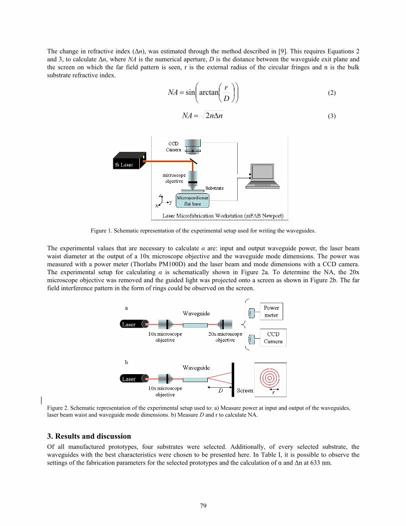
The change in refractive index (Δn), was estimated through the method described in [9]. This requires Equations 2 and 3, to calculate Δn, where NA is the numerical aperture, D is the distance between the waveguide exit plane and the screen on which the far field pattern is seen, r is the external radius of the circular fringes and n is the bulk substrate refractive index.

D

rNA arctansin (2)

nnNA 2 (3)

Figure 1. Schematic representation of the experimental setup used for writing the waveguides.

The experimental values that are necessary to calculate α are: input and output waveguide power, the laser beam waist diameter at the output of a 10x microscope objective and the waveguide mode dimensions. The power was measured with a power meter (Thorlabs PM100D) and the laser beam and mode dimensions with a CCD camera. The experimental setup for calculating α is schematically shown in Figure 2a. To determine the NA, the 20x microscope objective was removed and the guided light was projected onto a screen as shown in Figure 2b. The far field interference pattern in the form of rings could be observed on the screen.

Figure 2. Schematic representation of the experimental setup used to: a) Measure power at input and output of the waveguides, laser beam waist and waveguide mode dimensions. b) Measure D and r to calculate NA.

3. Results and discussion Of all manufactured prototypes, four substrates were selected. Additionally, of every selected substrate, the waveguides with the best characteristics were chosen to be presented here. In Table I, it is possible to observe the settings of the fabrication parameters for the selected prototypes and the calculation of α and Δn at 633 nm.

79

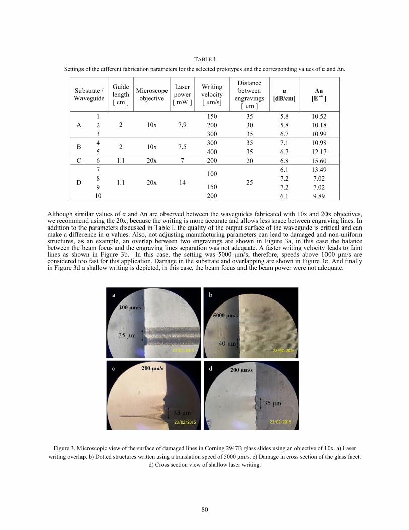
TABLE I

Settings of the different fabrication parameters for the selected prototypes and the corresponding values of α and Δn.

Substrate / Waveguide

Guide length [ cm ]

Microscope objective

Laser power [ mW ]

Writing velocity [ μm/s]

Distance between

engravings [ μm ]

α [dB/cm]

Δn [E -4 ]

A 1

2 10x 7.9 150 35 5.8 10.52

2 200 30 5.8 10.18 3 300 35 6.7 10.99

B 4

2 10x 7.5 300 35 7.1 10.98

5 400 35 6.7 12.17 C 6 1.1 20x 7 200 20 6.8 15.60

D

7

1.1 20x 14 100

25

6.1 13.49 8 7.2 7.02 9 150 7.2 7.02

10 200 6.1 9.89

Although similar values of α and Δn are observed between the waveguides fabricated with 10x and 20x objectives, we recommend using the 20x, because the writing is more accurate and allows less space between engraving lines. In addition to the parameters discussed in Table I, the quality of the output surface of the waveguide is critical and can make a difference in α values. Also, not adjusting manufacturing parameters can lead to damaged and non-uniform structures, as an example, an overlap between two engravings are shown in Figure 3a, in this case the balance between the beam focus and the engraving lines separation was not adequate. A faster writing velocity leads to faint lines as shown in Figure 3b. In this case, the setting was 5000 μm/s, therefore, speeds above 1000 μm/s are considered too fast for this application. Damage in the substrate and overlapping are shown in Figure 3c. And finally in Figure 3d a shallow writing is depicted, in this case, the beam focus and the beam power were not adequate.

Figure 3. Microscopic view of the surface of damaged lines in Corning 2947B glass slides using an objective of 10x. a) Laser writing overlap. b) Dotted structures written using a translation speed of 5000 μm/s. c) Damage in cross section of the glass facet.

d) Cross section view of shallow laser writing.

80

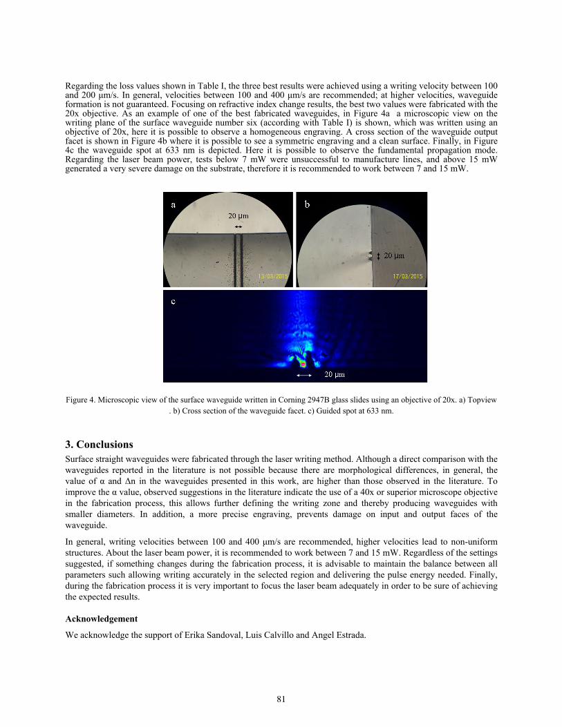
Regarding the loss values shown in Table I, the three best results were achieved using a writing velocity between 100 and 200 μm/s. In general, velocities between 100 and 400 μm/s are recommended; at higher velocities, waveguide formation is not guaranteed. Focusing on refractive index change results, the best two values were fabricated with the 20x objective. As an example of one of the best fabricated waveguides, in Figure 4a a microscopic view on the writing plane of the surface waveguide number six (according with Table I) is shown, which was written using an objective of 20x, here it is possible to observe a homogeneous engraving. A cross section of the waveguide output facet is shown in Figure 4b where it is possible to see a symmetric engraving and a clean surface. Finally, in Figure 4c the waveguide spot at 633 nm is depicted. Here it is possible to observe the fundamental propagation mode. Regarding the laser beam power, tests below 7 mW were unsuccessful to manufacture lines, and above 15 mW generated a very severe damage on the substrate, therefore it is recommended to work between 7 and 15 mW.

Figure 4. Microscopic view of the surface waveguide written in Corning 2947B glass slides using an objective of 20x. a) Topview . b) Cross section of the waveguide facet. c) Guided spot at 633 nm.

3. Conclusions Surface straight waveguides were fabricated through the laser writing method. Although a direct comparison with the waveguides reported in the literature is not possible because there are morphological differences, in general, the value of α and Δn in the waveguides presented in this work, are higher than those observed in the literature. To improve the α value, observed suggestions in the literature indicate the use of a 40x or superior microscope objective in the fabrication process, this allows further defining the writing zone and thereby producing waveguides with smaller diameters. In addition, a more precise engraving, prevents damage on input and output faces of the waveguide.

In general, writing velocities between 100 and 400 μm/s are recommended, higher velocities lead to non-uniform structures. About the laser beam power, it is recommended to work between 7 and 15 mW. Regardless of the settings suggested, if something changes during the fabrication process, it is advisable to maintain the balance between all parameters such allowing writing accurately in the selected region and delivering the pulse energy needed. Finally, during the fabrication process it is very important to focus the laser beam adequately in order to be sure of achieving the expected results. Acknowledgement

We acknowledge the support of Erika Sandoval, Luis Calvillo and Angel Estrada.

81

Numerical study on a photonic crystal waveguide that include a dispersive metamaterial

Héctor Pérez-Aguilar, Alberto Mendoza-Suárez

1. Avenida Francisco J. Múgica S/N Ciudad Universitaria, C.P. 58030,

Morelia, Michoacán, México. Corresponding author email: hiperezag@yahoo.com

ABSTRACT:

In this work we consider an electromagnetic system composed of two flat conductor surfaces and a periodic array of circular inclusions forming a photonic crystal waveguide. An integral numerical method was applied to determine the band structure of the system and the intensity field of its electromagnetic modes. We found that the variation of the filling fraction allow to control at a certain degree the photonic band structure of the system. We found interesting band structures that contain regions of nearly zero-dispersion and bandgaps. Although initially we considered that the medium inside the waveguide is vacuum, we also discuss the case of a dispersive metamaterial medium. Some numerical results show the presence of a plasmonic surface mode in the system proposed for TE polarization.

Key words: Photonic crystal waveguide, plasmonic surface mode, photonic band, integral equation method.

REFERENCES AND LINKS [1] Y. A. Vlasov, M. O'Boyle, H. F. Hamann and S. J. McNab, “Active control of slow light on a chip with photonic

crystal waveguides,” Nature 438, 65-69 (2005).

[2] A. Mendoza-Suárez, F. Villa-Villa and J. A. Gaspar-Armenta, “Plasmonic modes in a dispersive left handed material optical fiber,” Rev. Mex. Fis. 54, 82-86 (2008).

[3] A. Mendoza-Suárez, F. Villa-Villa, and J. A. Gaspar-Armenta, “Numerical method based on the solution of integral equations for the calculation of the band structure and reflectance of one- and two-dimensional photonic crystals,” J. Opt. Soc. Am. B 23, 2249-2256 (2006).

[4] A. Mendoza-Suárez, F. Villa-Villa, and J. A. Gaspar-Armenta, “Band structure of two-dimensional photonic crystals that include dispersive left-handed materials and dielectrics in the unit cell,” J. Opt. Soc. Am. B 24, 3091-3098 (2007).

[5] H. I. Pérez, E. R. Méndez, C. I. Valencia, and J. A. Sánchez-Gil, “On the transmission of diffuse light through thick slits,” J. Opt. Soc. Am. A 26, 909-918 (2009).

[6] J. B. Pendry, A. J. Holden, D. J. Robbins, and W. J. Stewart, “Low frequency plasmons in thin-wire structures,” Journal of Physics: Condensed Matter 10, 4785-4809 (1998).

[7] R. Ruppin, “Surface polaritons and extinction properties of a left-handed material cylinder,” J. Phys.: Condens. Matter 16, 5991-5998 (2004).

1. Introduction Recent development in photonic crystal waveguides has created interest among scientists from different fields [1]. The photonic crystals that constitute periodic arrays of different materials with a unit cell of dimension on the order

82

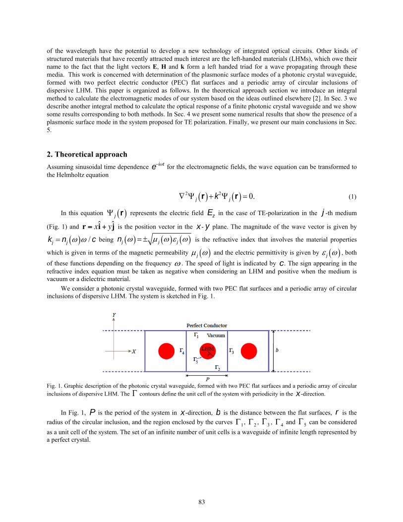
of the wavelength have the potential to develop a new technology of integrated optical circuits. Other kinds of structured materials that have recently attracted much interest are the left-handed materials (LHMs), which owe their name to the fact that the light vectors E, H and k form a left handed triad for a wave propagating through these media. This work is concerned with determination of the plasmonic surface modes of a photonic crystal waveguide, formed with two perfect electric conductor (PEC) flat surfaces and a periodic array of circular inclusions of dispersive LHM. This paper is organized as follows. In the theoretical approach section we introduce an integral method to calculate the electromagnetic modes of our system based on the ideas outlined elsewhere [2]. In Sec. 3 we describe another integral method to calculate the optical response of a finite photonic crystal waveguide and we show some results corresponding to both methods. In Sec. 4 we present some numerical results that show the presence of a plasmonic surface mode in the system proposed for TE polarization. Finally, we present our main conclusions in Sec. 5.

2. Theoretical approach

Assuming sinusoidal time dependence eit for the electromagnetic fields, the wave equation can be transformed to the Helmholtz equation

2 j r k2 j r 0. (1)

In this equation j r represents the electric field Ez in the case of TE-polarization in the j -th medium

(Fig. 1) and is the position vector in the x - y plane. The magnitude of the wave vector is given by

kj nj / c being nj j j is the refractive index that involves the material properties

which is given in terms of the magnetic permeability j and the electric permittivity is given by j , both

of these functions depending on the frequency . The speed of light is indicated by c. The sign appearing in the refractive index equation must be taken as negative when considering an LHM and positive when the medium is vacuum or a dielectric material.

We consider a photonic crystal waveguide, formed with two PEC flat surfaces and a periodic array of circular inclusions of dispersive LHM. The system is sketched in Fig. 1.

Fig. 1. Graphic description of the photonic crystal waveguide, formed with two PEC flat surfaces and a periodic array of circular inclusions of dispersive LHM. The contours define the unit cell of the system with periodicity in the x -direction.

In Fig. 1, P is the period of the system in x -direction, b is the distance between the flat surfaces, r is the

radius of the circular inclusion, and the region enclosed by the curves 1, 2 , 3 , 4 and 5 can be considered

as a unit cell of the system. The set of an infinite number of unit cells is a waveguide of infinite length represented by a perfect crystal.

83

The periodicity in the x -direction is a symmetry condition that is specially considered. Due to this property and the form of the differential equation Eq. (1) the Bloch theorem can be applied for the x -direction. In this way the following expression can be derived

xP, y exp ikP x, y , (2)

where k is the one-dimensional Bloch vector.

To determine the modes we have to find the dispersion relation k . With this in mind, let us consider a

Green's function for a two-dimensional geometry that can be used to solve the Helmholtz equation. The Green's

function considered is G(r,r ) iH01 r r / c , where H0

1 z is the Hankel function of the first kind and

zero order. Considering the geometry of the unit cell shown in Fig. 1 and applying the two-dimensional second Green's theorem for the functions and G we obtain the expression

(3)

being r 1 if r is inside the unit cell and r 0 otherwise. d s is the differential arc's length, n is the

outward normal vector to C , and the observation point r is infinitesimally separated of contour C outer to the unit cell.

To solve numerically Eq. (3), we divide the curve C in five segments 1, 2 , 3 , 4 and 5 (see Fig. 1)

and take a sampling Xn X sn , Yn Y sn along the each curve. Besides these considerations, we take into

account the boundary condition at the PEC surfaces (with curves 1 and 2 ) and applying Ec. (2) we obtain the

equations n4 exp ikP n

3 , and n4 exp ikP n

3 . In this way, Eq. (3) can be represented

numerically in terms of a homogeneous system of N algebraic equations as follows:

n1

N1

Lmn 1 1 n 1

n1

N2

Lmn 2 1 n 2

n1

N3

Lmn 3 1 exp ikP Lmn 4

1 n 3

n1

N3

Nmn 3 1 exp ikP Nmn 4

1 n 3 n1

N5

Lmn 5 1 n 5

n1

N5

Nmn 5 1 n 5 0,

(4)

n1

N5

Lmn 5 2 2

0

n 5 n1

N5

Nmn 5 2 n 5 0, (5)

for m1, 2,..., N N5 in Eq. (4) and m N N5 1,..., N in Eq. (5). In the Eqs. (4) and (5) the source

functions n j and n j represent numerically the field and its normal derivative, besides, the subscripts

n j , j 1, 2,3, 4, 5 denote the n-th point along the j contour. The matrix element Lmn j 1, 2

and Nmn j 1, 2

are

given in Refs. [2-4].

84

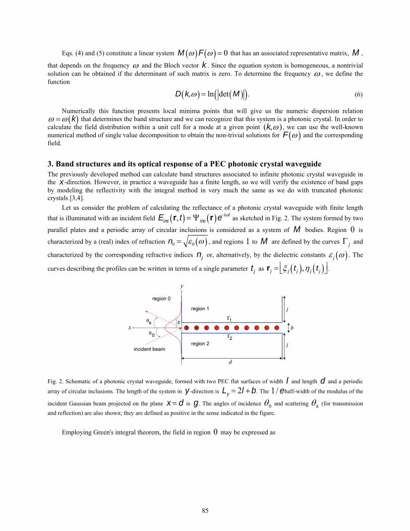
Eqs. (4) and (5) constitute a linear system M F 0 that has an associated representative matrix, M ,

that depends on the frequency and the Bloch vector k . Since the equation system is homogeneous, a nontrivial solution can be obtained if the determinant of such matrix is zero. To determine the frequency , we define the function

D k, ln det M . (6)

Numerically this function presents local minima points that will give us the numeric dispersion relation k that determines the band structure and we can recognize that this system is a photonic crystal. In order to calculate the field distribution within a unit cell for a mode at a given point (k,), we can use the well-known numerical method of single value decomposition to obtain the non-trivial solutions for F and the corresponding field.

3. Band structures and its optical response of a PEC photonic crystal waveguide The previously developed method can calculate band structures associated to infinite photonic crystal waveguide in the x -direction. However, in practice a waveguide has a finite length, so we will verify the existence of band gaps by modeling the reflectivity with the integral method in very much the same as we do with truncated photonic crystals [3,4].

Let us consider the problem of calculating the reflectance of a photonic crystal waveguide with finite length

that is illuminated with an incident field Einc r, t inc r eit as sketched in Fig. 2. The system formed by two

parallel plates and a periodic array of circular inclusions is considered as a system of M bodies. Region 0 is

characterized by a (real) index of refraction n0 0 , and regions 1 to M are defined by the curves j and

characterized by the corresponding refractive indices nj or, alternatively, by the dielectric constants j . The

curves describing the profiles can be written in terms of a single parameter t j as r j j t j , j t j .

Fig. 2. Schematic of a photonic crystal waveguide, formed with two PEC flat surfaces of width l and length d and a periodic

array of circular inclusions. The length of the system in y -direction is Ly 2l b. The 1 / ehalf-width of the modulus of the

incident Gaussian beam projected on the plane x d is g . The angles of incidence 0 and scattering s (for transmission

and reflection) are also shown; they are defined as positive in the sense indicated in the figure.

Employing Green's integral theorem, the field in region 0 may be expressed as

85

0 (r ) inc0 (r ) 1

4 j1

M

j

G0 (r, t j )

nj

0 (t j )G0 r, t j 0 (t j )

nj

dt j , (7)

where /nj j t j /y j

t j /x is the (nonnormalized) normal derivative operator and G0 (r, t j ) is

a suitable Green function for region 0 [5]. In this expression, inc0 (r ) represents the incident field, and the sum of

the integrals represents the scattered field. The source functions 0 (t j ) and 0 (t j ) /nj , which represent the

values of the field and its normal derivative evaluated on the surface.

Following the same steps for region j , the field ( j ) (r ) may be expressed as

j (r ) ( j )(r ) 1

4 j

Gj (r,t j )

nj

( j ) (t j )Gj (r,t j ) j (t j )

nj

dt j , (8)

where j (r ) is unity for points inside medium j and zero otherwise, and Gj (r, t j ) is the Green function for

medium j .

Eqs. (7) and (8) constitute a set of 2M coupled integral equations that can be solved numerically to obtain the boundary values for the field and its normal derivative on the surface of the scattering bodies. Details of the discretization of these equations and their conversion into matrix equations can be found in Ref. [5].

In order to treat the problem with the numerical method given above, some considerations must be made. Since the size of the system is finite, to avoid edge effects we illuminate it with a tapered Gaussian beam whose intercept with the plane of the waveguide has a half-width g . This parameter must be smaller than the total length of the

system Ly 2l b, but much larger than the width of the aperture b (see Fig. 2).

With these considerations, the incident field can be expressed in terms of its angular spectrum A(q,ky),

inc(x, y) 1

2 n0 /c

n0 /c

A(q,ky)exp{i qx0 (q)y }dq, (9)

where 0 (q) [( / c)2 q2 ]1/2 with e0 (q) 0 and m0 (q) 0 . In our case we choose

A(q | ky) 0 gexp g2 (q ky)2 / 4 i0 (q)d , (10)

being 0 a constant with appropriate units. The parameter ky n0 ( / c)sin0 , where 0 represents the angle of

incidence (see Fig. 2).

With this incident field we can find that the total power crossing the area LyLz , where Lz is a length in the z

direction, is given by

86

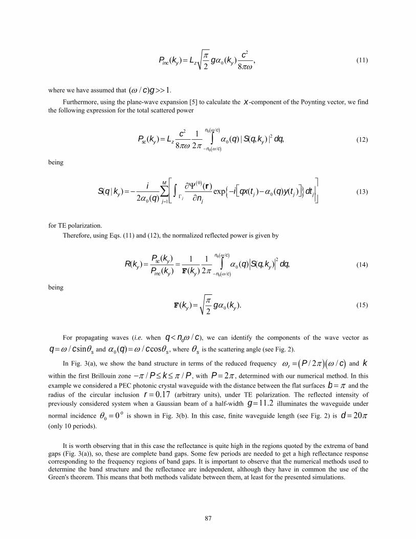
Pinc(ky) Lz

2

g0 (ky)c2

8, (11)

where we have assumed that ( / c)g1.

Furthermore, using the plane-wave expansion [5] to calculate the x -component of the Poynting vector, we find the following expression for the total scattered power

Psc(ky) Lz

c2

81

2 n0 /c

n0 /c

0 (q) | S(q,ky) |2 dq, (12)

being

S(q | ky) i

20 (q) j1

M

j 0 (r )

nj

exp i qx(t j )0 (q)y(t j ) dt j

(13)

for TE polarization.

Therefore, using Eqs. (11) and (12), the normalized reflected power is given by

R(ky) Psc(ky)

Pinc(ky) 1

F(ky)

1

2 n0 /c

n0 /c

0 (q) S(q, ky)2dq, (14)

being

F(ky) 2

g0 (ky). (15)

For propagating waves (i.e. when q no / c), we can identify the components of the wave vector as

q / csins and 0 (q) / ccoss , where s is the scattering angle (see Fig. 2).

In Fig. 3(a), we show the band structure in terms of the reduced frequency r P / 2 / c and k

within the first Brillouin zone / P k / P , with P 2 , determined with our numerical method. In this

example we considered a PEC photonic crystal waveguide with the distance between the flat surfaces b and the radius of the circular inclusion r 0.17 (arbitrary units), under TE polarization. The reflected intensity of previously considered system when a Gaussian beam of a half-width g11.2 illuminates the waveguide under

normal incidence 0 0 o is shown in Fig. 3(b). In this case, finite waveguide length (see Fig. 2) is d 20

(only 10 periods).

It is worth observing that in this case the reflectance is quite high in the regions quoted by the extrema of band gaps (Fig. 3(a)), so, these are complete band gaps. Some few periods are needed to get a high reflectance response corresponding to the frequency regions of band gaps. It is important to observe that the numerical methods used to determine the band structure and the reflectance are independent, although they have in common the use of the Green's theorem. This means that both methods validate between them, at least for the presented simulations.

87

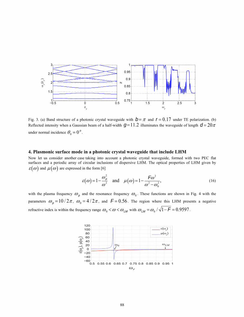
Fig. 3. (a) Band structure of a photonic crystal waveguide with b and r 0.17 under TE polarization. (b)

Reflected intensity when a Gaussian beam of a half-width g11.2 illuminates the waveguide of length d 20under normal incidence 0 0 o .

4. Plasmonic surface mode in a photonic crystal waveguide that include LHM Now let us consider another case taking into account a photonic crystal waveguide, formed with two PEC flat surfaces and a periodic array of circular inclusions of dispersive LHM. The optical properties of LHM given by

and are expressed in the form [6]

1p

2

2and 1 F 2

2 02, (16)

with the plasma frequency p and the resonance frequency 0 . These functions are shown in Fig. 4 with the

parameters p 10 / 2 , 0 4 / 2 , and F 0.56 . The region where this LHM presents a negative

refractive index is within the frequency range 0 LM with LM 0 / 1F 0.9597 .

88

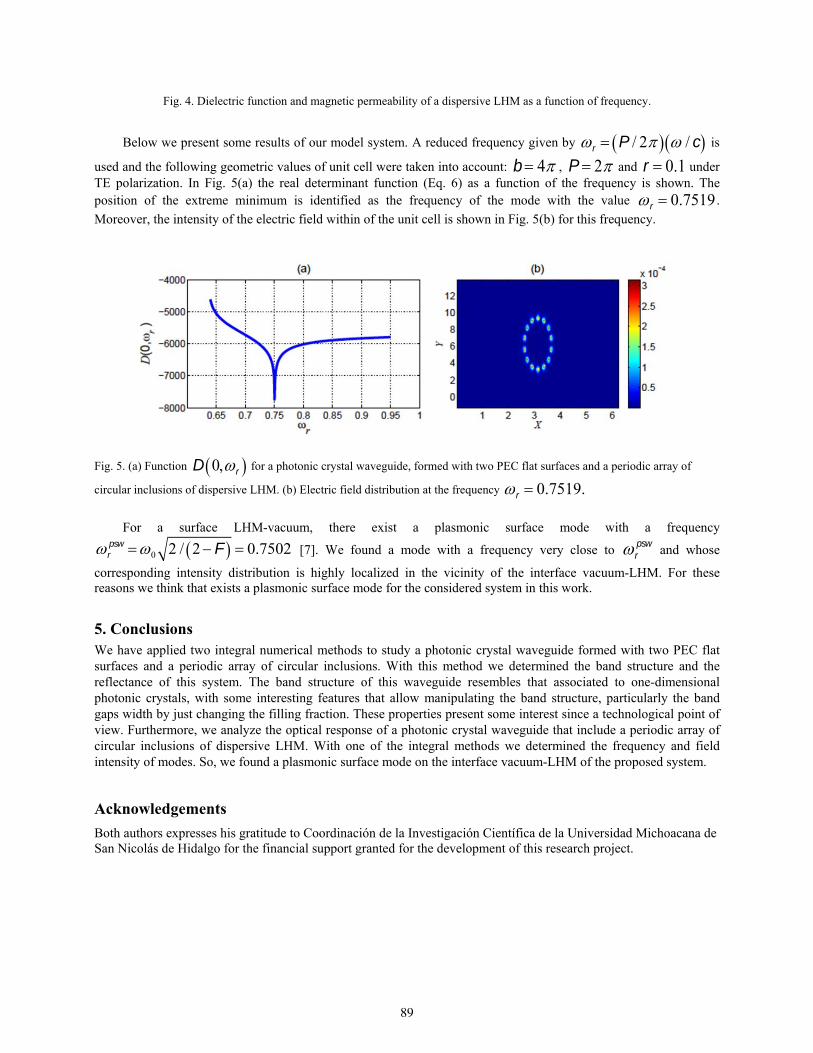
Fig. 4. Dielectric function and magnetic permeability of a dispersive LHM as a function of frequency.

Below we present some results of our model system. A reduced frequency given by r P / 2 / c is

used and the following geometric values of unit cell were taken into account: b 4 , P 2 and r 0.1 under TE polarization. In Fig. 5(a) the real determinant function (Eq. 6) as a function of the frequency is shown. The position of the extreme minimum is identified as the frequency of the mode with the value r 0.7519.

Moreover, the intensity of the electric field within of the unit cell is shown in Fig. 5(b) for this frequency.

Fig. 5. (a) Function D 0,r for a photonic crystal waveguide, formed with two PEC flat surfaces and a periodic array of

circular inclusions of dispersive LHM. (b) Electric field distribution at the frequency r 0.7519.

For a surface LHM-vacuum, there exist a plasmonic surface mode with a frequency

rpsw 0 2 / 2F 0.7502 [7]. We found a mode with a frequency very close to r

psw and whose

corresponding intensity distribution is highly localized in the vicinity of the interface vacuum-LHM. For these reasons we think that exists a plasmonic surface mode for the considered system in this work.

5. Conclusions We have applied two integral numerical methods to study a photonic crystal waveguide formed with two PEC flat surfaces and a periodic array of circular inclusions. With this method we determined the band structure and the reflectance of this system. The band structure of this waveguide resembles that associated to one-dimensional photonic crystals, with some interesting features that allow manipulating the band structure, particularly the band gaps width by just changing the filling fraction. These properties present some interest since a technological point of view. Furthermore, we analyze the optical response of a photonic crystal waveguide that include a periodic array of circular inclusions of dispersive LHM. With one of the integral methods we determined the frequency and field intensity of modes. So, we found a plasmonic surface mode on the interface vacuum-LHM of the proposed system.

Acknowledgements

Both authors expresses his gratitude to Coordinación de la Investigación Científica de la Universidad Michoacana de San Nicolás de Hidalgo for the financial support granted for the development of this research project.

89

Integrated Vibration Detection System Based on an Optical Fiber Sensor

J. A. Herrera-Estévez (1), L. E. Alanís-Carranza(1), J.A. Álvarez-Chávez(2), G E Sandoval-Romero(3) , A. Gómez-Vieyra(4), G.G. Pérez-Sánchez*(4)

1. Tecnológico de Estudios Superiores de Coacalco,Av. 16 de Septiembre #54, Col. Cabecera Municipal,

Coacalco de Berriozábal, Edo. México. 2. Centro de Investigación e Innovación Tecnológica -IPN, Cerrada de CECATI S/N,Col. Santa Catarina, c.p.

02250 D.F. Mexico 3. Centro de Ciencias Aplicadas y Desarrollo Tecnológico, Universidad Nacional Autónoma de

Mexico, Apartado Postal 70-186, México D. F., 04510, Mexico. 4. Departamento de Ciencias Básicas, Universidad Autónoma Metropolitana, Unidad Azcapotzalco, Av. San

Pablo 180, Azcapotzalco, Col. Reynosa Tamaulipas, Azcapotzalco México D. F. 02200 Corresponding author email: *ggps@correo.azc.uam.mx

ABSTRACT:

This work presents an early development stage of a vibration detection system based on optical fiber sensor. The sensor array consists on a pump laser diode at 980 nm, an erbium doped fiber section spliced to a SMF28 fiber and a long period fiber grating onto de fiber. The detection array is an opto-electronic system with a photodetection stage and proprietary software to observe the signal responses in both, frequency and time domains. In the time domain with vibration, the signal increases an average voltage up to 95% into the 1300 nm to 1650 nm spectrum.

Key words: Vibration, fiber sensor

REFERENCES AND LINKS [1] Hong-Nan Lia, Dong-Sheng Lia, Gang-Bing Song, “Recent applications of fiber optic sensors to health monitoring in civil engineering”

[2] Lopez-Higuera, J.M., Rodriguez Cobo, L., Quintela Incera, A. , Cobo, A.,“Fiber Optic Sensors in Structural Health Monitoring”, Journal of Lightwave Technology, (Volume:29 , Issue: 4 )

[3] Ivan Lujo, Pavo Klokoc, Tin Komljenovic, Marko Bosiljevac, Zvonimir Sipus,“Fiber-Optic Vibration Sensor Based On Multimode Fiber”, Radioengineering, Vol. 17, No. 2, June 2008 93 [4] Bravo H., Ponce L., Suárez G. y Zúniga R., "Potencial Sísmico de México", DDF, 1-66, 1988. Fundación ICA, "Catálogo de temblores que han afectado al valle de México. Siglo XIV al XX". Ed. Limusa, 1992.

1. Introduction The detection of internal and external vibrational changes in structures is currently an important area of theoretical and experimental studies in fields of structural health, building damage prevention and mechanical stress reduction. The main goals of these investigations are the detection, prediction and in some cases the correction of mechanical and structural failures on furniture, buildings and historical monuments as this could save human lives [1-3]. It is well known that Mexico City is located in a seismic region and it has been affected by strong earthquakes for many years. The seismic sources which affect Mexico City are: the local tremors originated near or inside the basin, the so-called Acambay tremors originated in the North American plate and medium-deep tremors caused by the oceanic Cocos plate in the Pacific, besides the subduction earthquakes originated under sea [4].

90

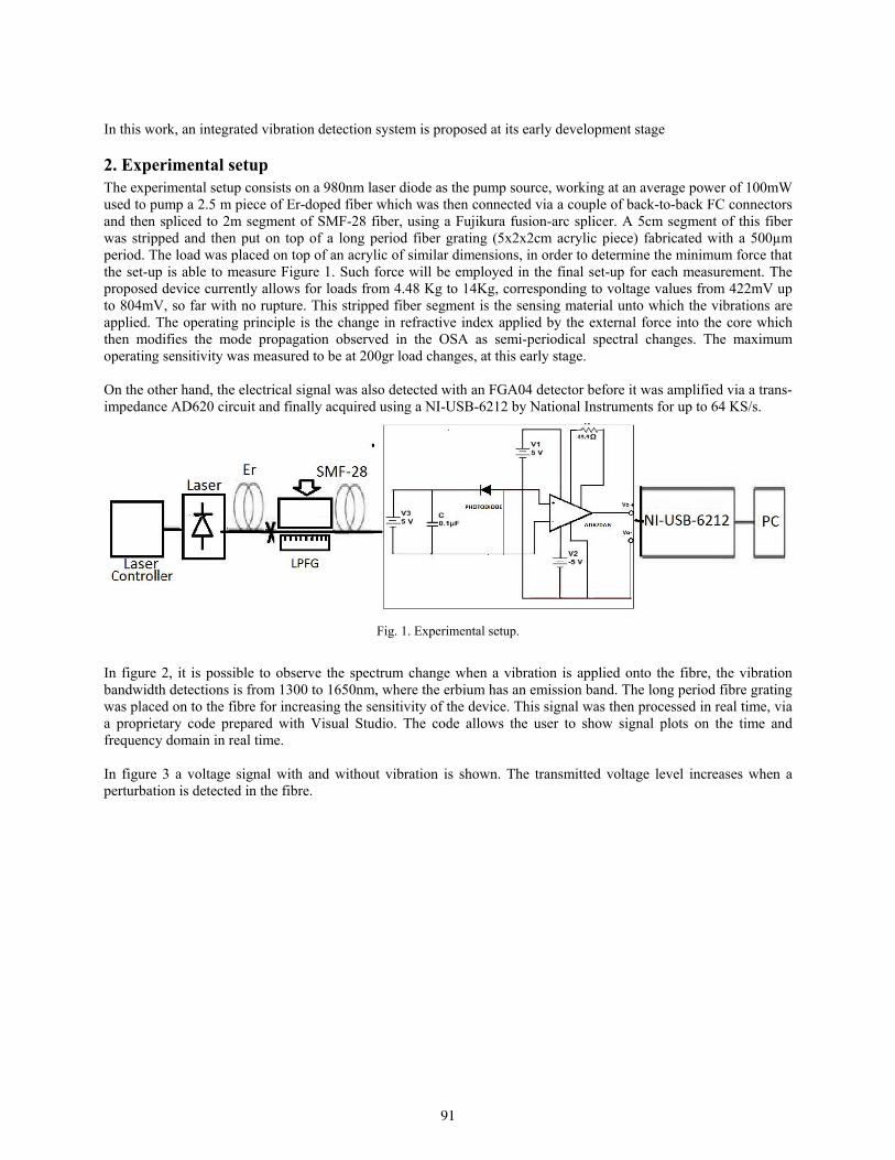
In this work, an integrated vibration detection system is proposed at its early development stage 2. Experimental setup The experimental setup consists on a 980nm laser diode as the pump source, working at an average power of 100mW used to pump a 2.5 m piece of Er-doped fiber which was then connected via a couple of back-to-back FC connectors and then spliced to 2m segment of SMF-28 fiber, using a Fujikura fusion-arc splicer. A 5cm segment of this fiber was stripped and then put on top of a long period fiber grating (5x2x2cm acrylic piece) fabricated with a 500µm period. The load was placed on top of an acrylic of similar dimensions, in order to determine the minimum force that the set-up is able to measure Figure 1. Such force will be employed in the final set-up for each measurement. The proposed device currently allows for loads from 4.48 Kg to 14Kg, corresponding to voltage values from 422mV up to 804mV, so far with no rupture. This stripped fiber segment is the sensing material unto which the vibrations are applied. The operating principle is the change in refractive index applied by the external force into the core which then modifies the mode propagation observed in the OSA as semi-periodical spectral changes. The maximum operating sensitivity was measured to be at 200gr load changes, at this early stage. On the other hand, the electrical signal was also detected with an FGA04 detector before it was amplified via a trans-impedance AD620 circuit and finally acquired using a NI-USB-6212 by National Instruments for up to 64 KS/s.

Fig. 1. Experimental setup.

In figure 2, it is possible to observe the spectrum change when a vibration is applied onto the fibre, the vibration bandwidth detections is from 1300 to 1650nm, where the erbium has an emission band. The long period fibre grating was placed on to the fibre for increasing the sensitivity of the device. This signal was then processed in real time, via a proprietary code prepared with Visual Studio. The code allows the user to show signal plots on the time and frequency domain in real time. In figure 3 a voltage signal with and without vibration is shown. The transmitted voltage level increases when a perturbation is detected in the fibre.

91

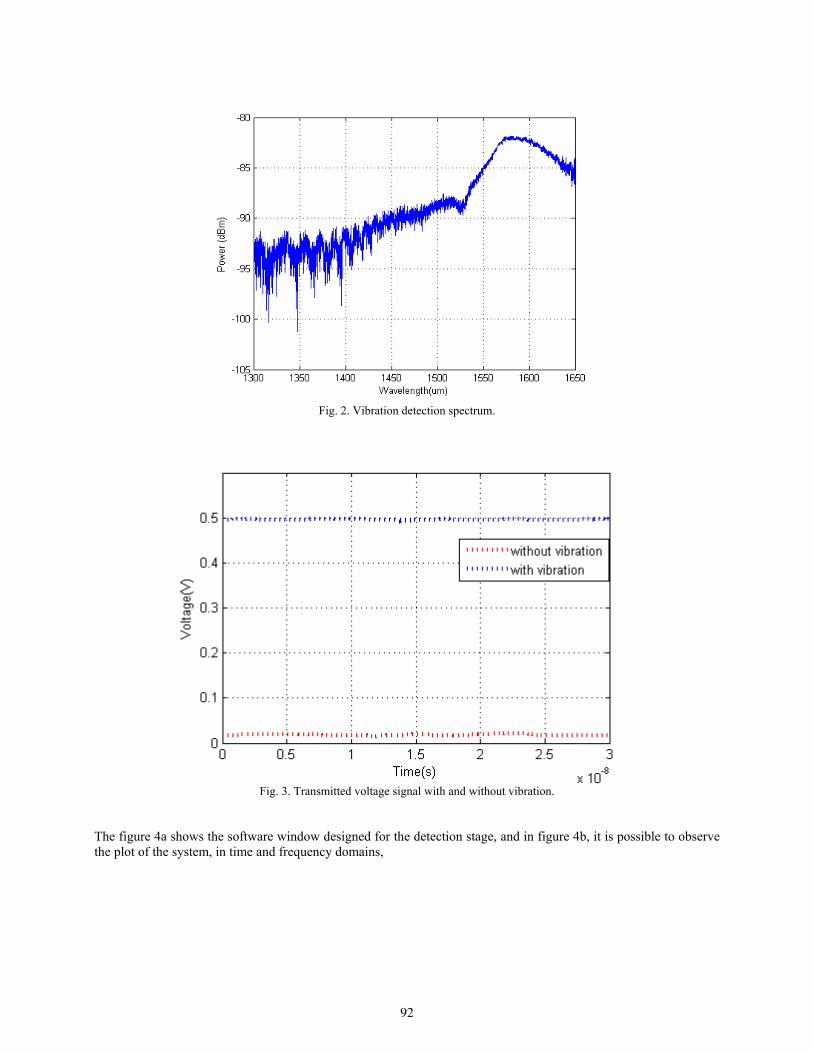
Fig. 2. Vibration detection spectrum.

Fig. 3. Transmitted voltage signal with and without vibration.

The figure 4a shows the software window designed for the detection stage, and in figure 4b, it is possible to observe the plot of the system, in time and frequency domains,

92

Fig. 4a. Detection SW.

Fig. 4b. Detection SW.

3. Conclusions This work presents an early development stage of a vibration detection system based on optical fiber sensor. The vibration detection spectrum was observed from 1300 nm to 1650 nm and the time signal response with vibration increases from 0.05 V to 0.5 V with the proposed array. A proprietary code was designed and implemented to plot the time domain and frequency spectrum at real time responses. The accuracy of the proposed device is still being studied as we still need to validate our measurements for different frequency ranges and loads. Acknowledgements

To UAM-Azc, CIITEC-IPN, TESCo and CCADET, for the facilities to develop this project.

93

Tunable upconversion emission and warm white in novel Yb3+/Er3+ codoped glass ceramic

J. A. Molina 1,2, A. Perez-Tiscareño 1,2, L. R. Palacios 1,2, H. Desirena 2, E. de la Rosa 2

1. División de Ciencias e Ingenierías, Universidad de Guanajuato, A.P. E-143, León Gto. C.P 37150 México

2. Centro de Investigaciones en Óptica, A.P. 1-948, León Gto. 37150 México Corresponding author email: hagdes@cio.mx

ABSTRACT:

Yb3+/Er3+ codoped fluoride glass ceramic doped with low rare earth concentration were prepared and the spectroscopic properties were analyzed. The glass ceramic were milled in a ball mill with a particle size from 60 nm to 1 µm. The samples were compared with NaYF4:20Yb3+/3Er3+ microcrystals (1-5 µm) under the same measurements conditions and the results show similar upconversion emission properties. The results show that color emission can be tuned from green to warm white when pump power excitation increase. The emission intensity is enough strong that is easily observed with the naked eye.

Key words: Upconversion, rare earth, microparticles, tunable upvonversion.

REFERENCES AND LINKS [1] G. Tian and et al, Mn2+ Dopant-Controlled Synthesis of NaYF4:Yb/Er Upconversion Nanoparticles for in vivo

Imaging and Drug Delivery, Adv. Mat. 24, 1226-1231 (2012)

[2] J. M. Meruga, W. M. Cross, P. S. May, Q. Luu, G. A. Crawford and J. J. Kellar, Security printing of covert quick response codes using upconverting nanoparticle inks, Nanotechnology 23, 395201 (2012).

[3] X. Huang, S. Han, W. Huang, X. Liu, Enhancing solar cell efficiency: the search for luminescent materials as spectral converters, Chem. Soc. Rev. 42,173 (2013)

[4] F. Vetrone, V. Mahalinggam and J. Capobianco, Near-Infrared-Blue Upconversion in Colloidal BaYF5:Tm3+,Yb3+ Nanocrystals, Chem. Mat. 21, 1847-1851 (2009).

[5] R. Liu and et al, Controlled synthesis and optical spectroscopy of lanthanide-doped KLaF4 nanocrystals, Nanoscale 4, 4485 (2012)

[6] Y. Ding and et al, Orthorhombic KSc2F7:Yb/Er nanorods: controlled synthesis and strong red upconversion emission, Nanoscale 5, 11928 (2013)

[7] J. C. Boyer and C. J. M. Van Veggel, Absolute quantum yield measurement of colloidal NaYF4:Er3+, Yb3+ upconverting nanoparticles, Nanoscale 2, 1417-1419 (2010).

[8] H. Desirena, E. De la Rosa, A. Schulzgen, and N. Peyghambarian, Er3+ and Yb3+ concentration effect in the spectroscopic properties and energy transfer in Yb3+/Er3+ codoped tellurite glasses, J. Phys. D: Appl. Phys. 41, 095102 (2008).

1. Introduction Visible upconversion emission from rare earth is of great interest due to the potential applications in biomedical application, security, solar cell and so on [1-3]. Intense blue-red and green-red upconversion, it has been demonstrated in several host matrixes [4-6]. However, to obtain the desired color the intensity ratios of red, green

94

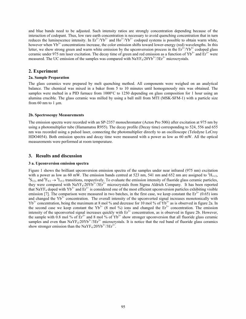
and blue bands need to be adjusted. Such intensity ratios are strongly concentration depending because of the interaction of codopant. Thus, low rare earth concentration is necessary to avoid quenching concentration that in turn reduces the luminescence intensity. In Er3+/Yb3+ and Ho3+/Yb3+ codoped systems is possible to obtain warm white, however when Yb3+ concentrations increase, the color emission shifts toward lower-energy (red) wavelengths. In this letter, we show strong green and warm white emission by the upconverssion process in the Er3+/Yb3+ codoped glass ceramic under 975 nm laser excitation. The decay time of green and red emission as a function of Yb3+ and Er3+ were measured. The UC emission of the samples was compared with NaYF4:20Yb3+/3Er3+ microcrystals.

2. Experiment 2a. Sample Preparation

The glass ceramics were prepared by melt quenching method. All components were weighed on an analytical balance. The chemical was mixed in a baker from 5 to 10 minutes until homogenously mix was obtained. The samples were melted in a PID furnace from 1000C to 1250 depending on glass composition for 1 hour using an alumina crucible. The glass ceramic was milled by using a ball mill from MTI (MSK-SFM-1) with a particle size from 60 nm to 1 µm.

2b. Spectroscopy Measurements

The emission spectra were recorded with an SP-2357 monochromator (Acton Pro 500i) after excitation at 975 nm by using a photomultiplier tube (Hamamatsu R955). The decay profile (Decay time) corresponding to 524, 556 and 655 nm was recorded using a pulsed laser, connecting the photomultiplier directly to an oscilloscope (Teledyne LeCroy HDO4054). Both emission spectra and decay time were measured with a power as low as 60 mW. All the optical measurements were performed at room temperature.

3. Results and discussion

3 a. Upconversion emission spectra

Figure 1 shows the brilliant upconversion emission spectra of the samples under near infrared (975 nm) excitation with a power as low as 60 mW. The emission bands centred at 523 nm, 541 nm and 652 nm are assigned to 2H11/2, 4S3/2, and 4F9/2 4I15/2 transitions, respectively. To evaluate the emission intensity of fluoride glass ceramic particles, they were compared with NaYF4:20Yb3+/3Er3+ microcrystals from Sigma Aldrich Company. It has been reported that NaYF4 doped with Yb3+ and Er3+ is considered one of the most efficient upconversion particles exhibiting visible emission [7]. The comparison were measured in two batches, in the first case, we keep constant the Er3+ (0.65) ions and changed the Yb3+ concentration. The overall intensity of the upconverted signal increases monotonically with Yb3+ concentration, being the maximum at 8 mol % and decrease for 10 mol % of Yb3+ as is observed in figure 2a. In the second case we keep constant the Yb3+ (8 mol %) ions and changed the Er3+ concentration. The emission intensity of the upconverted signal increases quickly with Er3+ concentration, as is observed in figure 2b. However, the sample with 0.8 mol % of Er3+ and 8 mol % of Yb3+ show stronger upconversion that all fluoride glass ceramic samples and even than NaYF4:20Yb3+/3Er3+ microcrystals. It is notice that the red band of fluoride glass ceramics show stronger emission than the NaYF4:20Yb3+/3Er3+.

95

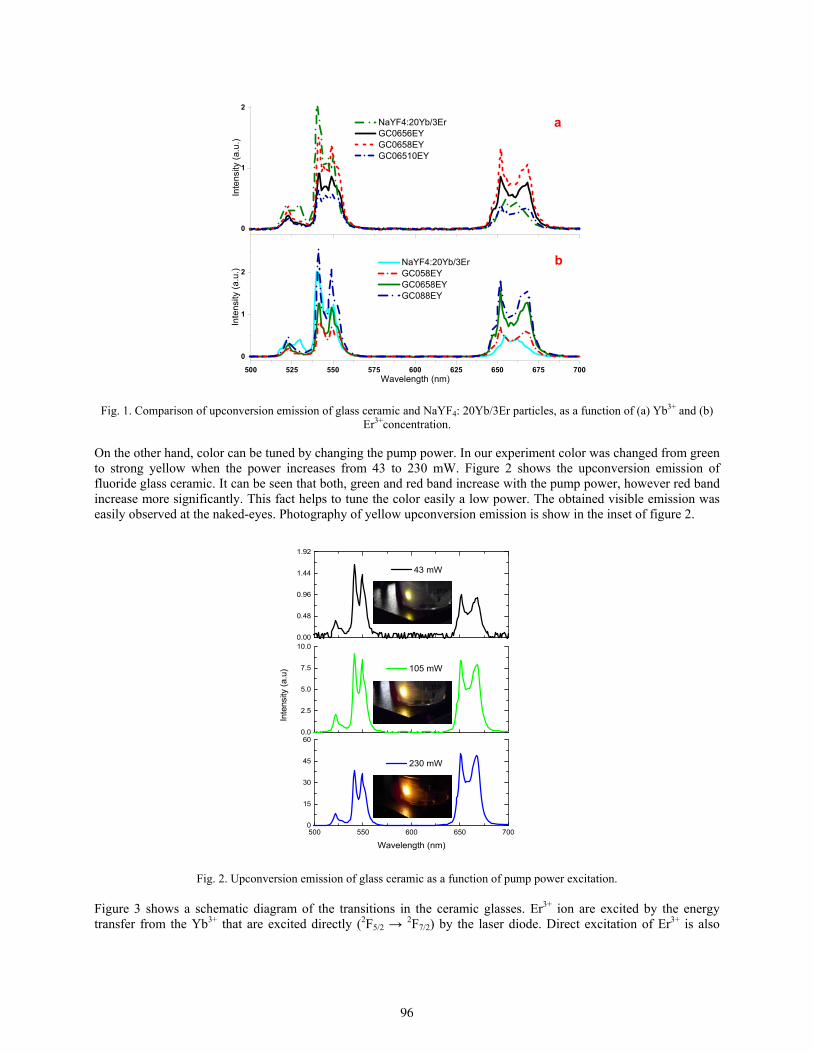
500 525 550 575 600 625 650 675 700

0

1

2 NaYF4:20Yb/3Er GC058EY GC0658EY GC088EY

Inte

nsity

(a.

u.)

Wavelength (nm)

0

1

2

b

NaYF4:20Yb/3Er GC0656EY GC0658EY GC06510EY

Inte

nsi

ty (

a.u

.)

a

Fig. 1. Comparison of upconversion emission of glass ceramic and NaYF4: 20Yb/3Er particles, as a function of (a) Yb3+ and (b) Er3+concentration.

On the other hand, color can be tuned by changing the pump power. In our experiment color was changed from green to strong yellow when the power increases from 43 to 230 mW. Figure 2 shows the upconversion emission of fluoride glass ceramic. It can be seen that both, green and red band increase with the pump power, however red band increase more significantly. This fact helps to tune the color easily a low power. The obtained visible emission was easily observed at the naked-eyes. Photography of yellow upconversion emission is show in the inset of figure 2.

Fig. 2. Upconversion emission of glass ceramic as a function of pump power excitation.

Figure 3 shows a schematic diagram of the transitions in the ceramic glasses. Er3+ ion are excited by the energy transfer from the Yb3+ that are excited directly (2F5/2 → 2F7/2) by the laser diode. Direct excitation of Er3+ is also

500 550 600 650 7000

15

30

45

600.0

2.5

5.0

7.5

10.00.00

0.48

0.96

1.44

1.92

230 mW

Wavelength (nm)

105 mW

Inte

nsity

(a.

u)

43 mW

96

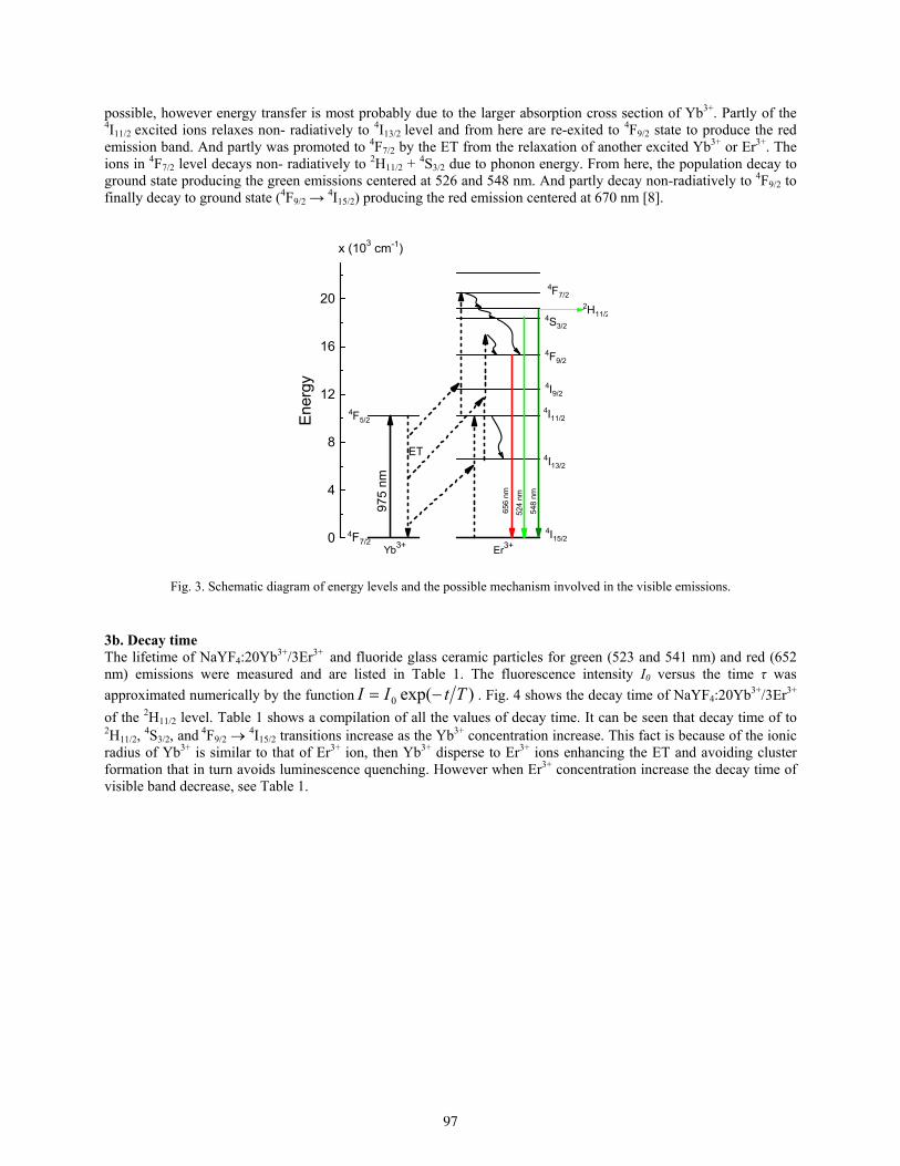
possible, however energy transfer is most probably due to the larger absorption cross section of Yb3+. Partly of the 4I11/2 excited ions relaxes non- radiatively to 4I13/2 level and from here are re-exited to 4F9/2 state to produce the red emission band. And partly was promoted to 4F7/2 by the ET from the relaxation of another excited Yb3+ or Er3+. The ions in 4F7/2 level decays non- radiatively to 2H11/2 + 4S3/2 due to phonon energy. From here, the population decay to ground state producing the green emissions centered at 526 and 548 nm. And partly decay non-radiatively to 4F9/2 to finally decay to ground state (4F9/2 → 4I15/2) producing the red emission centered at 670 nm [8].

0

4

8

12

16

20

524

nm

4F7/2

ET

Yb3+

975

nm

4I13/2

4I15/2

4I11/2

4I9/2

4F9/2

4S3/2

2H11/2E

nerg

y

Er3+

x (103 cm-1)

4F5/2

4F7/254

8 nm

656

nm

Fig. 3. Schematic diagram of energy levels and the possible mechanism involved in the visible emissions.

3b. Decay time The lifetime of NaYF4:20Yb3+/3Er3+

and fluoride glass ceramic particles for green (523 and 541 nm) and red (652 nm) emissions were measured and are listed in Table 1. The fluorescence intensity I0 versus the time τ was

approximated numerically by the function )exp(0 TtII . Fig. 4 shows the decay time of NaYF4:20Yb3+/3Er3+

of the 2H11/2 level. Table 1 shows a compilation of all the values of decay time. It can be seen that decay time of to 2H11/2,

4S3/2, and 4F9/2 4I15/2 transitions increase as the Yb3+ concentration increase. This fact is because of the ionic radius of Yb3+ is similar to that of Er3+ ion, then Yb3+ disperse to Er3+ ions enhancing the ET and avoiding cluster formation that in turn avoids luminescence quenching. However when Er3+ concentration increase the decay time of visible band decrease, see Table 1.

97

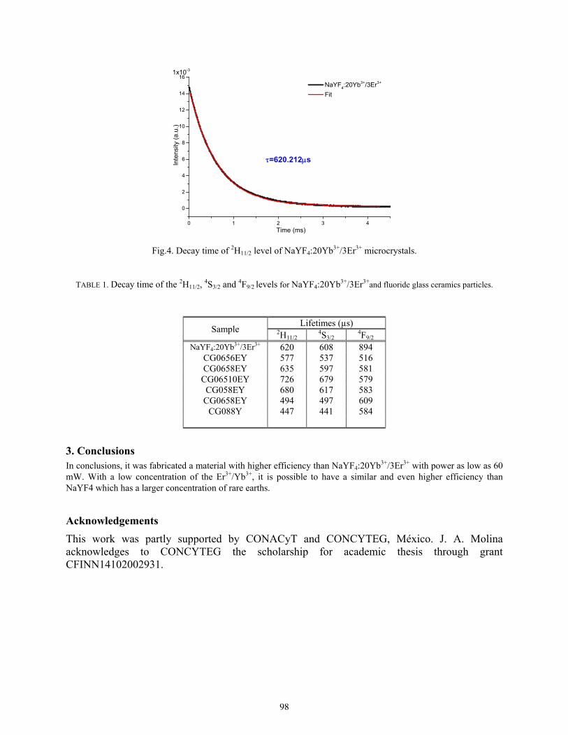
0 1 2 3 4

0

2

4

6

8

10

12

14

16

NaYF4:20Yb3+/3Er3+

Fit

Inte

nsity

(a.

u.)

Time (ms)

=620.212s

1x10-3

Fig.4. Decay time of 2H11/2 level of NaYF4:20Yb3+/3Er3+ microcrystals.

TABLE 1. Decay time of the 2H11/2, 4S3/2 and 4F9/2 levels for NaYF4:20Yb3+/3Er3+and fluoride glass ceramics particles.

Sample Lifetimes (µs)

2H11/2 4S3/2

4F9/2 NaYF4:20Yb3+/3Er3+ 620 608 894

CG0656EY 577 537 516 CG0658EY 635 597 581 CG06510EY 726 679 579 CG058EY 680 617 583

CG0658EY 494 497 609 CG088Y 447 441 584

3. Conclusions In conclusions, it was fabricated a material with higher efficiency than NaYF4:20Yb3+/3Er3+ with power as low as 60 mW. With a low concentration of the Er3+/Yb3+, it is possible to have a similar and even higher efficiency than NaYF4 which has a larger concentration of rare earths.

Acknowledgements

This work was partly supported by CONACyT and CONCYTEG, México. J. A. Molina acknowledges to CONCYTEG the scholarship for academic thesis through grant CFINN14102002931.

98

Development of numerical model to describe z-scan curves for medium thickness

Roman Torres Romero(1), Marcela Maribel Méndez Otero(1), Maximino Luis Arroyo Carrasco(1),

Marcelo David Iturbe Castillo (2)

1. Facultad de Ciencias Físico Matemáticas, BUAP 2. Instituto Nacional de Astrofisica Óptica y Electrónica, INAOE

roman_t_r@hotmail.com

ABSTRACT:

This word is based on the development of a numerical model which describe z-scan curves considering that the length material is much greater than 0z (Rayleigh distance). This material is studied as a set of photo-induced lens with variable F [1].

This model describe z-scan curves of numerical way with different lineal absorption coefficients and different sample lengths. The numerical results they were compared to experimental results getting a better approximation, these ones were made with isopropyl alcohol and organic dye; of results it was observed that transmittance peak increases as function of sample length. However for some value of the lineal absorption coefficient and the medium thickness, the maximum transmittance decreases, is observed also that the peaks are shifted to the left while the valleys remain almost in the same position.

Key words: Numerical model to describe z-scan curves

REFERENCES AND LINKS

[1] “Numerical study of the medium thickness in the z-scan technique”. I. Severiano Carrillo, M. Méndez Otero, M. L. Carrasco and M. D. Iturbe Castillo Journal of modern Optics, 2013, 60,248-254.

[2] Robert W. Boyd. Nonlinear Optics. Academic Press, INC. Tercera Edición.

[3] S. R. Friberg y P. W. Smith. Nonlinear optical glasses for ultrafast optical switches. IEEE J. Quantumm Electron., QE-23 (1987) 2089. [4] A. Owyoung. “Ellipse rotation studies in laser host materials.” IEEE J. Quantumm Electron., QE-9 (1973) 1064. [5] R. Adair L.L. Chase y S. A. Payne. Nonlinear refractive-index measurements of glasses using three-wave frequency mixing. J. Opt. Soc. Am., B4 (1987) 875. [6] W. E. Williams, M. J. Soileau y E. W. Van Stryland. Optical switching and n2 measurements in CS2. Opt. Comm., 50 (1984) 256. [7] M. Sheik-Bahae, A. A. Said y E. W. Van Stryland. High-sensitivity, single beam n2 measurements. Opt. Lett., 14 (1989) 955-957.

1. Introduction The nonlinear optic in recent years has been an important area of research because of its many potential applications in the area of photonics and optoelectronics. No doubt, these areas of research have and will continue to play an important role in technology. The nonlinear optic (ONL) studies the different phenomena that occur as a result of the

99

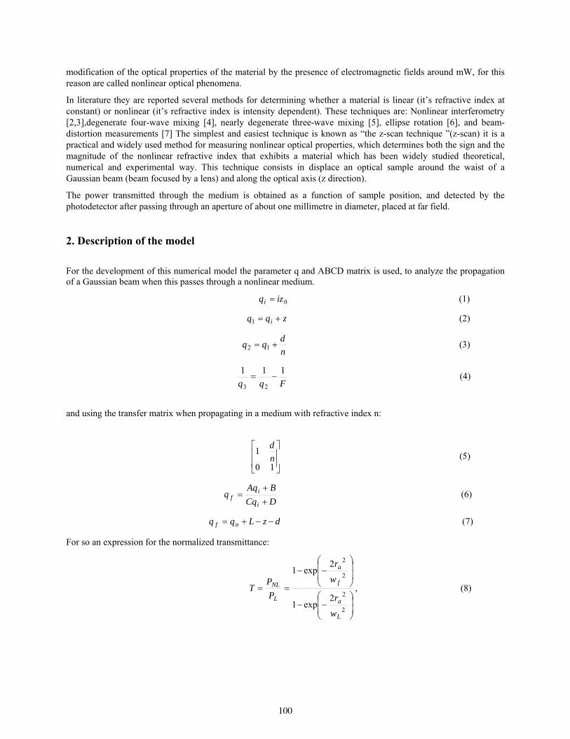
modification of the optical properties of the material by the presence of electromagnetic fields around mW, for this reason are called nonlinear optical phenomena.

In literature they are reported several methods for determining whether a material is linear (it’s refractive index at constant) or nonlinear (it’s refractive index is intensity dependent). These techniques are: Nonlinear interferometry [2,3],degenerate four-wave mixing [4], nearly degenerate three-wave mixing [5], ellipse rotation [6], and beam- distortion measurements [7] The simplest and easiest technique is known as “the z-scan technique ”(z-scan) it is a practical and widely used method for measuring nonlinear optical properties, which determines both the sign and the magnitude of the nonlinear refractive index that exhibits a material which has been widely studied theoretical, numerical and experimental way. This technique consists in displace an optical sample around the waist of a Gaussian beam (beam focused by a lens) and along the optical axis (z direction).

The power transmitted through the medium is obtained as a function of sample position, and detected by the photodetector after passing through an aperture of about one millimetre in diameter, placed at far field.

2. Description of the model

For the development of this numerical model the parameter q and ABCD matrix is used, to analyze the propagation of a Gaussian beam when this passes through a nonlinear medium.

0izqi (1)

zqq i 1 (2)

n

dqq 12 (3)

Fqq

111

23

(4)

and using the transfer matrix when propagating in a medium with refractive index n:

10

1n

d (5)

DCq

BAqq

i

if

(6)

dzLqq nf (7)

For so an expression for the normalized transmittance:

2

2

2

2

2exp1

2exp1

L

a

f

a

L

NL

w

r

w

r

P

PT , (8)

100

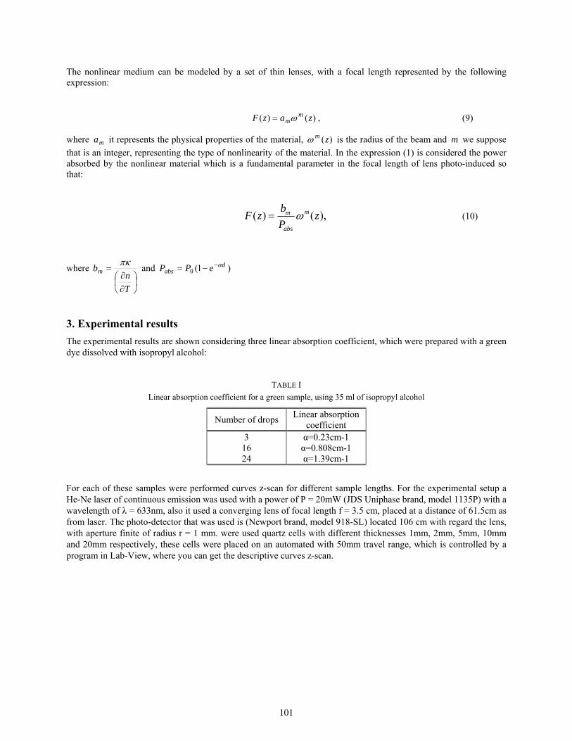
The nonlinear medium can be modeled by a set of thin lenses, with a focal length represented by the following expression:

)()( zazF mm , (9)

where ma it represents the physical properties of the material, )(zm is the radius of the beam and m we suppose

that is an integer, representing the type of nonlinearity of the material. In the expression (1) is considered the power absorbed by the nonlinear material which is a fundamental parameter in the focal length of lens photo-induced so that:

),()( zP

bzF m

abs

m (10)

where

T

nbm

and )1(0

dabs ePP

3. Experimental results

The experimental results are shown considering three linear absorption coefficient, which were prepared with a green dye dissolved with isopropyl alcohol:

TABLE I

Linear absorption coefficient for a green sample, using 35 ml of isopropyl alcohol

Number of drops Linear absorption

coefficient 3 α=0.23cm-1

16 α=0.808cm-1 24 α=1.39cm-1

For each of these samples were performed curves z-scan for different sample lengths. For the experimental setup a He-Ne laser of continuous emission was used with a power of P = 20mW (JDS Uniphase brand, model 1135P) with a wavelength of λ = 633nm, also it used a converging lens of focal length f = 3.5 cm, placed at a distance of 61.5cm as from laser. The photo-detector that was used is (Newport brand, model 918-SL) located 106 cm with regard the lens, with aperture finite of radius r = 1 mm. were used quartz cells with different thicknesses 1mm, 2mm, 5mm, 10mm and 20mm respectively, these cells were placed on an automated with 50mm travel range, which is controlled by a program in Lab-View, where you can get the descriptive curves z-scan.

101

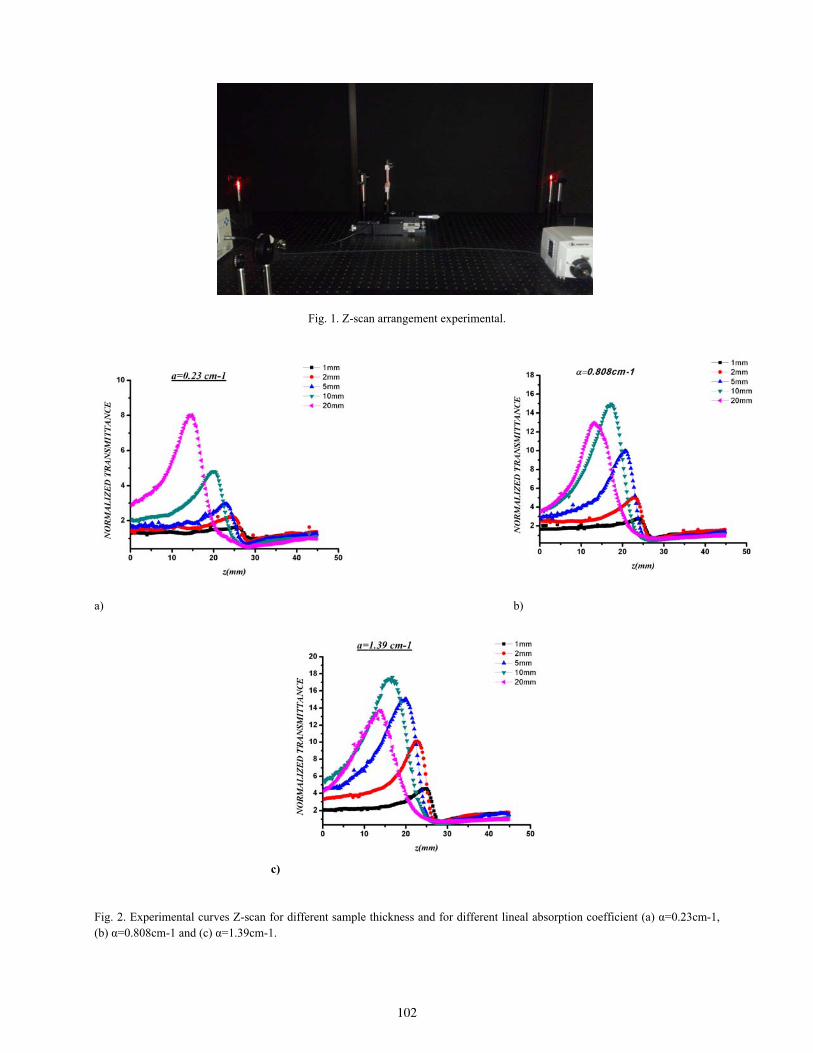
Fig. 1. Z-scan arrangement experimental.

a) b)

c)

Fig. 2. Experimental curves Z-scan for different sample thickness and for different lineal absorption coefficient (a) α=0.23cm-1, (b) α=0.808cm-1 and (c) α=1.39cm-1.

102

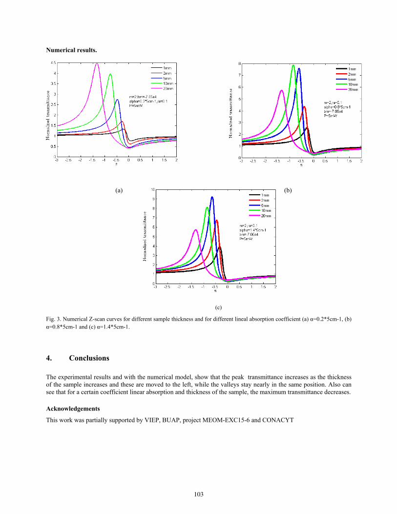
Numerical results.

(a) (b)

(c)

Fig. 3. Numerical Z-scan curves for different sample thickness and for different lineal absorption coefficient (a) α=0.2*5cm-1, (b) α=0.8*5cm-1 and (c) α=1.4*5cm-1.

4. Conclusions

The experimental results and with the numerical model, show that the peak transmittance increases as the thickness of the sample increases and these are moved to the left, while the valleys stay nearly in the same position. Also can see that for a certain coefficient linear absorption and thickness of the sample, the maximum transmittance decreases. Acknowledgements

This work was partially supported by VIEP, BUAP, project MEOM-EXC15-6 and CONACYT

103

Dependence of the photoluminescence properties of LiNbO3 single crystals on

the Zn doping concentration

J. G. Murillo1, A. Vega-Rios1, L. Carrasco-Valenzuela1, G. Herrera2, C. Alvarez-Herrera3, J. Castillo-Torres4

1. Centro de Investigación en Materiales Avanzados S. C., Miguel de Cervantes 120, Chihuahua 31136, Chihuahua México. 2. Cátedra CONACYT assigned to Department of Physics of Materials, Centro de Investigación en Materiales Avanzados S. C., Miguel de Cervantes 120, Chihuahua 31136, Chihuahua México. 3. Facultad de Ingeniería, Universidad Autónoma de Chihuahua, Circuito Universitario S/N, 31125 Chihuahua, Chihuahua, México. 4. Instituto de Física y Matemáticas, Universidad Tecnológica de la Mixteca, Huajuapan de León, Oaxaca, México.

Corresponding author email: jose.murillo@cimav.edu.mx

ABSTRACT:

This work reports the dependence of photoluminescence properties of LiNbO3 (LN) single crystals, on the Zn doping concentration. The samples were grown by Czochralski technique and were doped with zinc at concentration from 5 to 9 mol %. Structural and photoluminescence (PL) properties were studied by Raman, UV reflectance and fluorospectrometry, respectively. An extraordinary violet luminescence at 425 nm with excitation in UV region (380 nm) was observed. The emission peaks in PL spectra varied in amplitude and in wavelength position according to the level of concentration of Zn in the LN single crystals. It was found an optimal level concentration of Zn in the LN crystals studied in order to obtain a strong PL signal. The PL properties found in the LN crystals studied were related to the ratio of Li/Nb concentration.

Key words: Lithium niobate: Zinc, structural and photoluminescence properties.

REFERENCES AND LINKS [1] K. Buse, A. Adibi, D. Psaltis. Nature, 1998, 393, 665–668. [2] H. Qiao, J. Xu, G. Zhang, X. Zhang, Q. Sun, G. Zhang. Phys. Rev. B: Condens. Matter Mater. Phys., 2004, 70, 94101–94111. [3] J. Castillo-Torres. Phys. Status Solidi B 2013, 250, 1546–1550 [4] H. Zhen, L. C. Zhao, Y. H. Xu. Appl. Phys. B: Lasers Opt., 2003, 76, 655–659. [5] S. K. Kushwaha. K. K. Maurya, N. Vijayan, B. Kumar, R. Bhatt, S. Ganesamoorthy, G. Bhagavannarayana, Cryst. Eng. Comm, 2012, 14, 3297-3305. [6] H. Xu, D. Lee, S. B. Sinnott, V. Gopalan, V. Dierolf, S. R. Phillpot. Phys. Rev. B: Condens. Matter Mater. Phys., 2009, 80, 144104–144112. [7] J. G. Scott, S. Mailis, C. L. Sones, R. W. Eason. Appl. Phys. A: Mater. Sci. Process., 2004, 79, 691–696. [8] N. V. Sidorov, M. N. Palatnikov, V. T. Gabrielyan, P. G. Chufyrev. V. T. Kalinnikov. Inorg. Mater., 2007, 43, 60–67. [9] U. Schlarb, S. Klauer, M. Wesselmann, K. Betzler, M. Wohlccke, Appl. Phys. A: Solids Surf., 1993, 56, 311–315 [10] X. H. Zhen, W. S. Xu, C. Z. Zhao, L. C. Zhao, Y. H. Xu, Cryst. Res. Technol., 2002, 37, 976–982. [11] P. Günter, J.P. Huignard. Photorefractive Materials and their Applications, vols. 1 and 2 Springer, New York (2007) [12] P.D. Townsend, and K.A. Green, “Luminescence of LiNbO3” pp. 185-187, Ed. K.K. Wong, INSPEC,IEEE London UK, 2002.

104

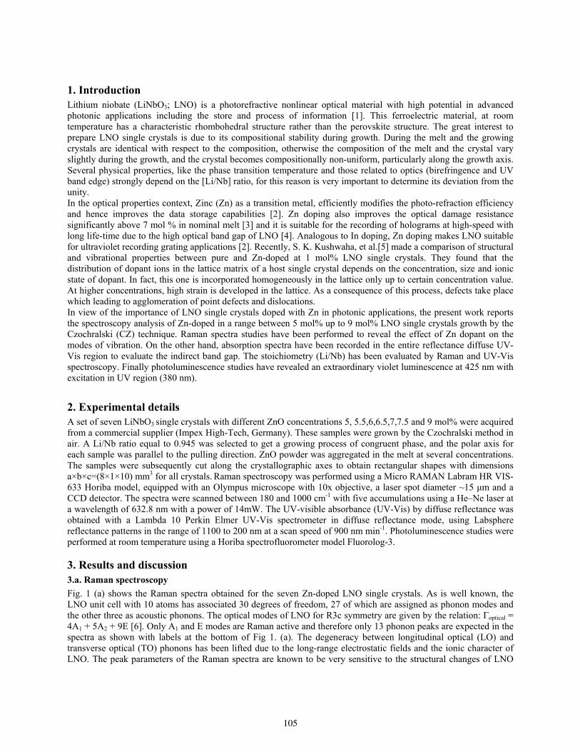
1. Introduction Lithium niobate (LiNbO3; LNO) is a photorefractive nonlinear optical material with high potential in advanced photonic applications including the store and process of information [1]. This ferroelectric material, at room temperature has a characteristic rhombohedral structure rather than the perovskite structure. The great interest to prepare LNO single crystals is due to its compositional stability during growth. During the melt and the growing crystals are identical with respect to the composition, otherwise the composition of the melt and the crystal vary slightly during the growth, and the crystal becomes compositionally non-uniform, particularly along the growth axis. Several physical properties, like the phase transition temperature and those related to optics (birefringence and UV band edge) strongly depend on the [Li/Nb] ratio, for this reason is very important to determine its deviation from the unity. In the optical properties context, Zinc (Zn) as a transition metal, efficiently modifies the photo-refraction efficiency and hence improves the data storage capabilities [2]. Zn doping also improves the optical damage resistance significantly above 7 mol % in nominal melt [3] and it is suitable for the recording of holograms at high-speed with long life-time due to the high optical band gap of LNO [4]. Analogous to In doping, Zn doping makes LNO suitable for ultraviolet recording grating applications [2]. Recently, S. K. Kushwaha, et al.[5] made a comparison of structural and vibrational properties between pure and Zn-doped at 1 mol% LNO single crystals. They found that the distribution of dopant ions in the lattice matrix of a host single crystal depends on the concentration, size and ionic state of dopant. In fact, this one is incorporated homogeneously in the lattice only up to certain concentration value. At higher concentrations, high strain is developed in the lattice. As a consequence of this process, defects take place which leading to agglomeration of point defects and dislocations. In view of the importance of LNO single crystals doped with Zn in photonic applications, the present work reports the spectroscopy analysis of Zn-doped in a range between 5 mol% up to 9 mol% LNO single crystals growth by the Czochralski (CZ) technique. Raman spectra studies have been performed to reveal the effect of Zn dopant on the modes of vibration. On the other hand, absorption spectra have been recorded in the entire reflectance diffuse UV-Vis region to evaluate the indirect band gap. The stoichiometry (Li/Nb) has been evaluated by Raman and UV-Vis spectroscopy. Finally photoluminescence studies have revealed an extraordinary violet luminescence at 425 nm with excitation in UV region (380 nm).

2. Experimental details A set of seven LiNbO3 single crystals with different ZnO concentrations 5, 5.5,6,6.5,7,7.5 and 9 mol% were acquired from a commercial supplier (Impex High-Tech, Germany). These samples were grown by the Czochralski method in air. A Li/Nb ratio equal to 0.945 was selected to get a growing process of congruent phase, and the polar axis for each sample was parallel to the pulling direction. ZnO powder was aggregated in the melt at several concentrations. The samples were subsequently cut along the crystallographic axes to obtain rectangular shapes with dimensions a×b×c=(8×1×10) mm3 for all crystals. Raman spectroscopy was performed using a Micro RAMAN Labram HR VIS-633 Horiba model, equipped with an Olympus microscope with 10x objective, a laser spot diameter ~15 μm and a CCD detector. The spectra were scanned between 180 and 1000 cm-1 with five accumulations using a He–Ne laser at a wavelength of 632.8 nm with a power of 14mW. The UV-visible absorbance (UV-Vis) by diffuse reflectance was obtained with a Lambda 10 Perkin Elmer UV-Vis spectrometer in diffuse reflectance mode, using Labsphere reflectance patterns in the range of 1100 to 200 nm at a scan speed of 900 nm min-1. Photoluminescence studies were performed at room temperature using a Horiba spectrofluorometer model Fluorolog-3. 3. Results and discussion 3.a. Raman spectroscopy

Fig. 1 (a) shows the Raman spectra obtained for the seven Zn-doped LNO single crystals. As is well known, the LNO unit cell with 10 atoms has associated 30 degrees of freedom, 27 of which are assigned as phonon modes and the other three as acoustic phonons. The optical modes of LNO for R3c symmetry are given by the relation: Γoptical = 4A1 + 5A2 + 9E [6]. Only A1 and E modes are Raman active and therefore only 13 phonon peaks are expected in the spectra as shown with labels at the bottom of Fig 1. (a). The degeneracy between longitudinal optical (LO) and transverse optical (TO) phonons has been lifted due to the long-range electrostatic fields and the ionic character of LNO. The peak parameters of the Raman spectra are known to be very sensitive to the structural changes of LNO

105

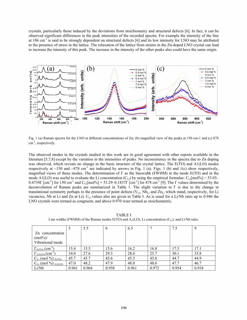
crystals, particularly those induced by the deviations from stoichiometry and structural defects [6]. In fact, it can be observed significant differences in the peak intensities of the recorded spectra. For example the intensity of the line at 186 cm-1 is said to be strongly dependent on structural defects [6] and its low intensity for LNO may be attributed to the presence of stress in the lattice. The relaxation of the lattice from strains in the Zn-doped LNO crystal can lead to increase the intensity of this peak. The increase in the intensity of the other peaks also could have the same origin.

Fig. 1 (a) Raman spectra for the LNO at different concentrations of Zn; (b) magnified view of the peaks at 150 cm-1 and (c) 878 cm-1, respectively.

The observed modes in the crystals studied in this work are in good agreement with other reports available in the literature [5,7,8] except by the variation in the intensities of peaks. No inconsistency in the spectra due to Zn doping was observed, which reveals no change in the basic structure of the crystal lattice. The E(TO) and A1(LO) modes respectively at ~150 and ~878 cm-1 are indicated by arrows in Fig. 1 (a). Figs. 1 (b) and 1(c) show respectively, magnified views of these modes. The determination of Γ as the linewidth (FWHM) in the mode E(TO) and in the mode A1(LO) was useful to evaluate the Li concentration (CLi) by using the empirical formulae: CLi[mol%] = 53.03–0.4739Γ [cm-1] for 150 cm-1 and CLi[mol%] = 53.29–0.1837Γ [cm-1] for 878 cm-1 [9]. The Γ values determined by the deconvolution of Raman peaks are summarized in Table 1. The slight variation in Γ is due to the change in translational symmetry perhaps to the presence of point defects (VLi, NbLi and ZnLi which stand, respectively, for Li vacancies, Nb at Li and Zn at Li). CLi values also are given in Table I. As is usual for a Li/Nb ratio up to 0.946 the LNO crystals were termed as congruent, and above 0.970 were termed as stoichiometric.

TABLE I Line widths (FWHM) of the Raman modes E(TO) and A1(LO), Li concentration (CLi), and Li/Nb ratio.

Zn concentration (mol%)/ Vibrational mode

5 5.5 6 6.5 7 7.5 9

ΓE(TO) (cm-1) 15.4 15.5 15.6 16.2 16.8 17.5 17.1 ΓA1(LO) (cm-1) 34.0 27.6 29.3 28.6 25.7 30.1 35.8 CLi (mol %) E(TO) 45.7 45.7 45.6 45.3 45.0 44.7 44.9 CLi (mol %) A1(LO) 47.0 48.2 47.9 48.0 48.6 47.7 46.7 Li/Nb 0.941 0.964 0.958 0.961 0.972 0.954 0.934

106

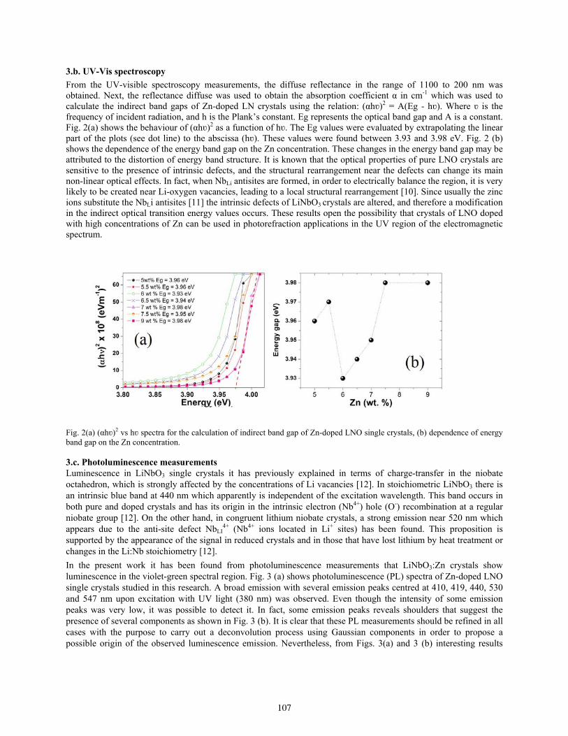
3.b. UV-Vis spectroscopy

From the UV-visible spectroscopy measurements, the diffuse reflectance in the range of 1100 to 200 nm was obtained. Next, the reflectance diffuse was used to obtain the absorption coefficient α in cm-1 which was used to calculate the indirect band gaps of Zn-doped LN crystals using the relation: (αhʋ)2 = A(Eg - hʋ). Where ʋ is the frequency of incident radiation, and h is the Plank’s constant. Eg represents the optical band gap and A is a constant. Fig. 2(a) shows the behaviour of (αhʋ)2 as a function of hʋ. The Eg values were evaluated by extrapolating the linear part of the plots (see dot line) to the abscissa (hʋ). These values were found between 3.93 and 3.98 eV. Fig. 2 (b) shows the dependence of the energy band gap on the Zn concentration. These changes in the energy band gap may be attributed to the distortion of energy band structure. It is known that the optical properties of pure LNO crystals are sensitive to the presence of intrinsic defects, and the structural rearrangement near the defects can change its main non-linear optical effects. In fact, when NbLi antisites are formed, in order to electrically balance the region, it is very likely to be created near Li-oxygen vacancies, leading to a local structural rearrangement [10]. Since usually the zinc ions substitute the NbLi antisites [11] the intrinsic defects of LiNbO3 crystals are altered, and therefore a modification in the indirect optical transition energy values occurs. These results open the possibility that crystals of LNO doped with high concentrations of Zn can be used in photorefraction applications in the UV region of the electromagnetic spectrum.

Fig. 2(a) (αhʋ)2 vs hʋ spectra for the calculation of indirect band gap of Zn-doped LNO single crystals, (b) dependence of energy band gap on the Zn concentration. 3.c. Photoluminescence measurements Luminescence in LiNbO3 single crystals it has previously explained in terms of charge-transfer in the niobate octahedron, which is strongly affected by the concentrations of Li vacancies [12]. In stoichiometric LiNbO3 there is an intrinsic blue band at 440 nm which apparently is independent of the excitation wavelength. This band occurs in both pure and doped crystals and has its origin in the intrinsic electron (Nb4+) hole (O-) recombination at a regular niobate group [12]. On the other hand, in congruent lithium niobate crystals, a strong emission near 520 nm which appears due to the anti-site defect NbLI

4+ (Nb4+ ions located in Li+ sites) has been found. This proposition is supported by the appearance of the signal in reduced crystals and in those that have lost lithium by heat treatment or changes in the Li:Nb stoichiometry [12].

In the present work it has been found from photoluminescence measurements that LiNbO3:Zn crystals show luminescence in the violet-green spectral region. Fig. 3 (a) shows photoluminescence (PL) spectra of Zn-doped LNO single crystals studied in this research. A broad emission with several emission peaks centred at 410, 419, 440, 530 and 547 nm upon excitation with UV light (380 nm) was observed. Even though the intensity of some emission peaks was very low, it was possible to detect it. In fact, some emission peaks reveals shoulders that suggest the presence of several components as shown in Fig. 3 (b). It is clear that these PL measurements should be refined in all cases with the purpose to carry out a deconvolution process using Gaussian components in order to propose a possible origin of the observed luminescence emission. Nevertheless, from Figs. 3(a) and 3 (b) interesting results

107

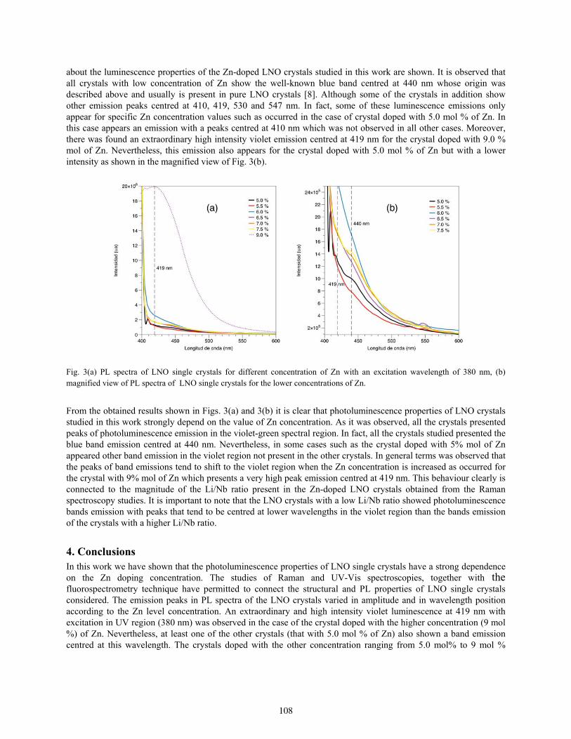
about the luminescence properties of the Zn-doped LNO crystals studied in this work are shown. It is observed that all crystals with low concentration of Zn show the well-known blue band centred at 440 nm whose origin was described above and usually is present in pure LNO crystals [8]. Although some of the crystals in addition show other emission peaks centred at 410, 419, 530 and 547 nm. In fact, some of these luminescence emissions only appear for specific Zn concentration values such as occurred in the case of crystal doped with 5.0 mol % of Zn. In this case appears an emission with a peaks centred at 410 nm which was not observed in all other cases. Moreover, there was found an extraordinary high intensity violet emission centred at 419 nm for the crystal doped with 9.0 % mol of Zn. Nevertheless, this emission also appears for the crystal doped with 5.0 mol % of Zn but with a lower intensity as shown in the magnified view of Fig. 3(b).

Fig. 3(a) PL spectra of LNO single crystals for different concentration of Zn with an excitation wavelength of 380 nm, (b) magnified view of PL spectra of LNO single crystals for the lower concentrations of Zn.

From the obtained results shown in Figs. 3(a) and 3(b) it is clear that photoluminescence properties of LNO crystals studied in this work strongly depend on the value of Zn concentration. As it was observed, all the crystals presented peaks of photoluminescence emission in the violet-green spectral region. In fact, all the crystals studied presented the blue band emission centred at 440 nm. Nevertheless, in some cases such as the crystal doped with 5% mol of Zn appeared other band emission in the violet region not present in the other crystals. In general terms was observed that the peaks of band emissions tend to shift to the violet region when the Zn concentration is increased as occurred for the crystal with 9% mol of Zn which presents a very high peak emission centred at 419 nm. This behaviour clearly is connected to the magnitude of the Li/Nb ratio present in the Zn-doped LNO crystals obtained from the Raman spectroscopy studies. It is important to note that the LNO crystals with a low Li/Nb ratio showed photoluminescence bands emission with peaks that tend to be centred at lower wavelengths in the violet region than the bands emission of the crystals with a higher Li/Nb ratio.

4. Conclusions In this work we have shown that the photoluminescence properties of LNO single crystals have a strong dependence on the Zn doping concentration. The studies of Raman and UV-Vis spectroscopies, together with the fluorospectrometry technique have permitted to connect the structural and PL properties of LNO single crystals considered. The emission peaks in PL spectra of the LNO crystals varied in amplitude and in wavelength position according to the Zn level concentration. An extraordinary and high intensity violet luminescence at 419 nm with excitation in UV region (380 nm) was observed in the case of the crystal doped with the higher concentration (9 mol %) of Zn. Nevertheless, at least one of the other crystals (that with 5.0 mol % of Zn) also shown a band emission centred at this wavelength. The crystals doped with the other concentration ranging from 5.0 mol% to 9 mol %

108

presented bands emission in the blue-green spectral region with peaks centred at 440, 530, and 547 nm. A blue-shift in the PL spectra of LNO crystals with an increasing on the Zn concentration was observed. This blue-shift in the PL spectra was related to the existence of a low Li/Nb ratio in the LNO crystals such as was obtained from the Raman studies performed to the samples. These results open the possibility that crystals of LNO doped with high concentrations of Zn can be used in photonic applications in the UV region of the electromagnetic spectrum.

Acknowledgements

The authors would like to express their thanks to M.Sc. L. de la Torre-Saenz and M.Sc. P. Pizá- Ruiz, from the Laboratorio Nacional de Nanotecnología (NaNoTeCh). G. Herrera-Pérez would like to thank for complementary support SNI I-CONACyT and Cátedra Grant No. 2563 of CONACyT México.

109

Influence of the Nonlocality of a Thin Media on Their Nonlinear Response

M. L. Arroyo Carrasco (1), B. A. Martínez Irivas (1), M. M Méndez Otero(1) and M. D Iturbe Castillo(2)

1. Facultad de Ciencias Físico-Matemáticas, Benemérita Universidad Autónoma de Puebla, Av. San Claudio y 18

Sur. Col San Manuel, C.P. 72570, Puebla, Puebla, México. 2. Instituto Nacional de Astrofísica, Óptica y Electrónica, Luis Enrique Erro # 1, C.P. 72840 Tonantzintla, Puebla,

México Corresponding author email: marroyo@fcfm.buap.mx

ABSTRACT:

In this work we present a model for a Gaussian beam transmitted through a thin nonlinear sample that takes into account the local or nonlocal character of the nonlinear interaction. We consider that the sample exhibits simultaneously nonlinear refraction and absorption. This model is adequate to describe z-scan curves and spatial self-phase modulation effect. The nonlocality of the interaction is described with an m parameter that measure if the width of the photo-induced nonlinear phase change at the output of the sample is smaller or bigger than the width of the input intensity profile. Key words: Nonlocal nonlinear interaction, z-scan, spatial self-phase modulation.

REFERENCES AND LINKS [1] J.P. Gordon, R.C.C. Leite, R.S. Moore, S.P.S. Porto and J.R. Whinnery, “Long- transient effects in lasers with

inserted liquid samples,” J. Appl. Phys., 36(1), 3-8(1965).

[2] M. Sheik-Bahae, A.A. Said and E.W. Van Stryland, “High-sensitivity, single-beam n2 measurements,” Opt. Lett., 14(17), 955-957 (1989).

[3] M. Sheik-Bahae, A.A. Said, T.H. Wei, D.J. Hagan and E.W. Van Stryland, “Sensitive measurement of optical nonlinearities using a single beam,” IEEE J. Quant. Electron., 26(4), 760-769 (1990).

[4] D. Weaire, B.S. Wherrett, D.A.B. Miller and S.D. Smith, “Effect of low-power nonlinear refraction on laser-beam propagation in InSb,” Opt. Lett., 4(10), 331–333 (1979).

[5] S. Hughes, B. S. Wherrett, “Fast Fourier Transform techniques for efficient simulation of z-scan measurements,” J. Opt. Soc. Am. B, 12, 1888-1893 (1979).

[6] E. V. Garcia Ramirez, M. L. Arroyo Carrasco, M. M. Mendez Otero, E. Reynoso Lara, S. Chavez-Cerda and M. D. Iturbe Castillo, “Z-scan and spatial self-phase modulation of a Gaussian beam in a thin nonlocal nonlinear media,” J. Opt., 13, 085203(10pp) (2011).

[7] A. Balbuena Ortega, M.L. Arroyo Carrasco, M.M. Méndez Otero, E. Reynoso Lara, E.V. García Ramírez and M.D. Iturbe Castillo, “Analytical expressions for z-scan with arbitrary phase change in thin nonlocal nonlinear media”, Opt. Express, 22(23), 27932-27941 (2014).

1. Introduction The far field diffraction pattern due to spatial self-phase modulation when a Gaussian beam is transmitted through a thin nonlinear sample was one of the nonlinear effects studied in the earlier times of nonlinear optics [1]. The z-scan technique, proposed by Sheik-Bahae et al. [2, 3], is a widely used method to evaluate the nonlinear refraction, in the closed aperture configuration, and the nonlinear absorption, in the open aperture configuration. In this technique the

110

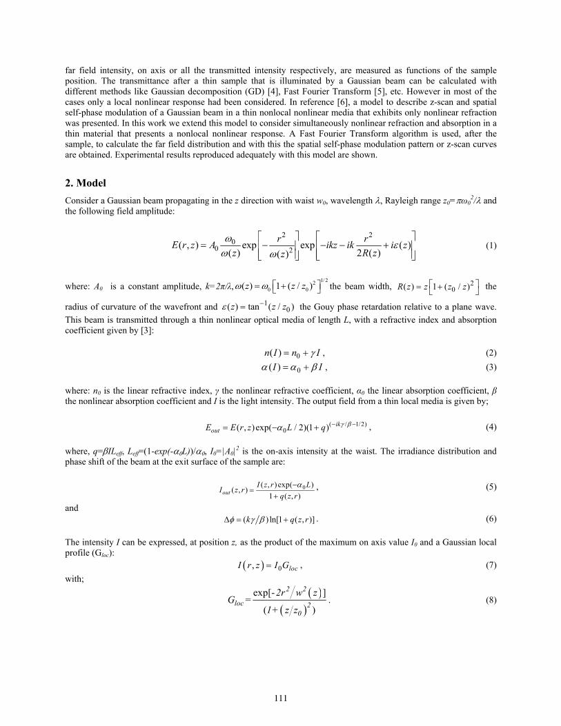
far field intensity, on axis or all the transmitted intensity respectively, are measured as functions of the sample position. The transmittance after a thin sample that is illuminated by a Gaussian beam can be calculated with different methods like Gaussian decomposition (GD) [4], Fast Fourier Transform [5], etc. However in most of the cases only a local nonlinear response had been considered. In reference [6], a model to describe z-scan and spatial self-phase modulation of a Gaussian beam in a thin nonlocal nonlinear media that exhibits only nonlinear refraction was presented. In this work we extend this model to consider simultaneously nonlinear refraction and absorption in a thin material that presents a nonlocal nonlinear response. A Fast Fourier Transform algorithm is used, after the sample, to calculate the far field distribution and with this the spatial self-phase modulation pattern or z-scan curves are obtained. Experimental results reproduced adequately with this model are shown.

2. Model

Consider a Gaussian beam propagating in the z direction with waist w0, wavelength , Rayleigh range z0=ω02/ and

the following field amplitude:

2 2

00 2

( , ) exp exp ( )( ) 2 ( )( )

r rE r z A ikz ik i z

z R zz

(1)

where: A0 is a constant amplitude, k=2π/λ,1/22

0 0( ) 1 ( / )z z z the beam width, 20( ) 1 ( / )R z z z z the

radius of curvature of the wavefront and 10( ) tan ( / )z z z the Gouy phase retardation relative to a plane wave.

This beam is transmitted through a thin nonlinear optical media of length L, with a refractive index and absorption coefficient given by [3]:

0( )n I n I , (2)

0( )I I , (3)

where: n0 is the linear refractive index, γ the nonlinear refractive coefficient, α0 the linear absorption coefficient, β the nonlinear absorption coefficient and I is the light intensity. The output field from a thin local media is given by;

( / 1/2)0( , )exp( / 2)(1 ) ik

outE E r z L q , (4)

where, q=ILeff, Leff=(1-exp(-L))/, I0=|A0|

2 is the on-axis intensity at the waist. The irradiance distribution and phase shift of the beam at the exit surface of the sample are:

0( , ) exp( )( , )

1 ( , )outI z r L

I z rq z r

, (5)

and ( ) ln[1 ( , )]k q z r . (6)

The intensity I can be expressed, at position z, as the product of the maximum on axis value I0 and a Gaussian local profile (Gloc):

0, locI r z I G , (7)

with;

exp[- ]=

( )

2 2

loc 20

2r w zG

1+ z z. (8)

111

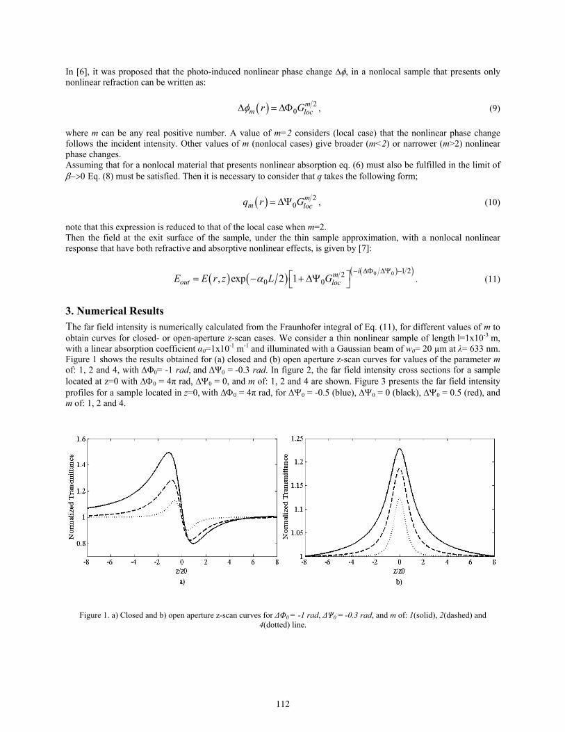
In [6], it was proposed that the photo-induced nonlinear phase change , in a nonlocal sample that presents only nonlinear refraction can be written as:

20

mm locr G , (9)

where m can be any real positive number. A value of m=2 considers (local case) that the nonlinear phase change follows the incident intensity. Other values of m (nonlocal cases) give broader (m<2) or narrower (m>2) nonlinear phase changes. Assuming that for a nonlocal material that presents nonlinear absorption eq. (6) must also be fulfilled in the limit of Eq. (8) must be satisfied. Then it is necessary to consider that q takes the following form;

20

mm locq r G , (10)

note that this expression is reduced to that of the local case when m=2. Then the field at the exit surface of the sample, under the thin sample approximation, with a nonlocal nonlinear response that have both refractive and absorptive nonlinear effects, is given by [7]:

0 0 1 22

0 0, exp 2 1im

out locE E r z L G

. (11)

3. Numerical Results

The far field intensity is numerically calculated from the Fraunhofer integral of Eq. (11), for different values of m to obtain curves for closed- or open-aperture z-scan cases. We consider a thin nonlinear sample of length l=1x10-3 m, with a linear absorption coefficient α0=1x10-1 m-1 and illuminated with a Gaussian beam of w0= 20 µm at λ= 633 nm. Figure 1 shows the results obtained for (a) closed and (b) open aperture z-scan curves for values of the parameter m of: 1, 2 and 4, with ΔΦ0= -1 rad, and ΔΨ0 = -0.3 rad. In figure 2, the far field intensity cross sections for a sample located at z=0 with 0 = 4π rad, 0 = 0, and m of: 1, 2 and 4 are shown. Figure 3 presents the far field intensity profiles for a sample located in z=0, with 0 = 4π rad, for 0 = -0.5 (blue), 0 = 0 (black), 0 = 0.5 (red), and m of: 1, 2 and 4.

Figure 1. a) Closed and b) open aperture z-scan curves for ΔΦ0 = -1 rad, ΔΨ0 = -0.3 rad, and m of: 1(solid), 2(dashed) and 4(dotted) line.

112

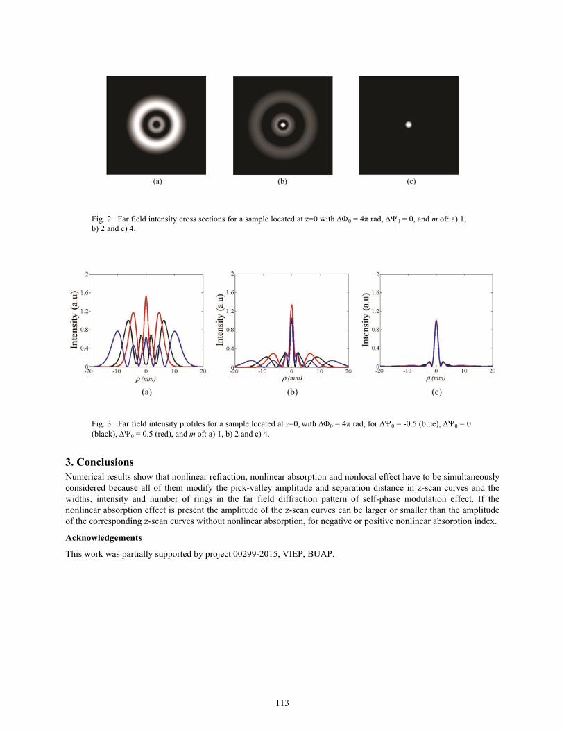
Fig. 2. Far field intensity cross sections for a sample located at z=0 with 0 = 4π rad, 0 = 0, and m of: a) 1, b) 2 and c) 4.

Fig. 3. Far field intensity profiles for a sample located at z=0, with 0 = 4π rad, for 0 = -0.5 (blue), 0 = 0 (black), 0 = 0.5 (red), and m of: a) 1, b) 2 and c) 4.

3. Conclusions Numerical results show that nonlinear refraction, nonlinear absorption and nonlocal effect have to be simultaneously considered because all of them modify the pick-valley amplitude and separation distance in z-scan curves and the widths, intensity and number of rings in the far field diffraction pattern of self-phase modulation effect. If the nonlinear absorption effect is present the amplitude of the z-scan curves can be larger or smaller than the amplitude of the corresponding z-scan curves without nonlinear absorption, for negative or positive nonlinear absorption index.

Acknowledgements

This work was partially supported by project 00299-2015, VIEP, BUAP.

113

Linear and Nonlinear Optical Properties of a Cobalt(III)-Salen Complex

M. G. Quintero Téllez (1), R. Mcdonald (2), M. L. Arroyo Carrasco (3), M. M. Méndez Otero (3), M. D. Iturbe Castillo (4), J. L. Alcántara Flores (5) and Y. Reyes Ortega (5)

1. Facultad de Ciencias Químicas, Benemérita Universidad Autónoma de Puebla, Av. San Claudio y 18 Sur, Col.

San Manuel, C.P. 72570, Puebla, Pue., México. 2. Department of Chemical and Materials Engineering, University of Alberta, Edmonton, Alberta, Canada T6G

2G6.3 3. Facultad de Ciencias Físico Matemáticas, Benemérita Universidad Autónoma de Puebla, Av. San Claudio y 18

Sur, Col. San Manuel, C.P. 72570, Puebla, Pue., México. 4. Instituto Nacional de Astrofísica, Óptica y Electrónica, Luis Enrique Erro # 1, C.P. 72840, Tonantzintla, Puebla,

México. 5. Centro de Química, Instituto de Ciencias, Benemérita Universidad Autónoma de Puebla, Av. San Claudio y 18

Sur, Col. San Manuel, C.P. 72570, Puebla, Pue., México.

guadalupe.quintero@correo.buap.mx

ABSTRACT:

In this work we present some linear and nonlinear optical properties characterization of the complex [Co2(III)(2,2’-{azanidediylbis(ethane-2,1-diylnitrilomethylylidene)}diphenolate)2] dimethyl sulfoxide disolvate. The closed aperture z-scan curves of DMSO solution of the complex indicates that it has a negative nonlinear refractive index and the open aperture z-scan trace do not show nonlinear absorption. The nonlinear optical response is closed related to the chemical structure compound and can be explained on the base of electron accepting/donating ability of the molecules group.

Key words: Cobalt(III)-salen complex; Nonlinear optical response; Z-scan technique

REFERENCES AND LINKS [1] O. A. Turanova, G. I. Ivanova, L. G. Gafiyatullin, T. A. Ivanova, L. V. Mingalieva, A. N. Turanov, and I. V.

Ovchinnikov, Russian Journal of General Chemistry, “Preparation and Liquid_Crystalline Properties of Mono- and Binuclear Complexes of Fe(III) with Pentadentate Schiff´s Base”, 84, 2174-2179, (2014).

[2] P. Ghosh, A. R. Chowdhury, S. Kr. Saha, M. Ghosh, M, Pal, N. Chandra Murmu, P. Benerjee, “Synthesis and characterization of redox non-innocent cobalt(III) complexes of a O,N,O donor ligand: Radical generation, semi-conductivity, antibacterial and anticancer activities”, Inorg. Chim. Acta, 429, 99-108 (2015).

[3] G. Zhang S. Wang, J. S. Ma, G. Yang, J. S. Yang, “Syntheses, characterization and third-order nonlinear optical properties of a class of thiazolylazo-based metal complexes”, Inorg. Chim. Acta, 384, 97-104, (2012).

[4] G. Quintero-Tellez, C. M. González Álvarez, S. Bernès, J. L. Alcántara-Flores and Y. Reyes-Ortega, “Bis{-2,2’-[3-azapentane-1,5-diyl) bis(nitrilomethylidyne)]diphenolato}dicopper(II) dimethyl sulfoxide disolvate”, Acta Cryst. E64, m631-m632, (2008).

[5] R.A. D. Wentworth and T.S. Piper, “A cristal field fodel for the spectral relationships in monoacidopentammine and diacidotetraammine complexes of cobalt(III)”, Inorg. Chem., 1965, 4, 709-714.

114

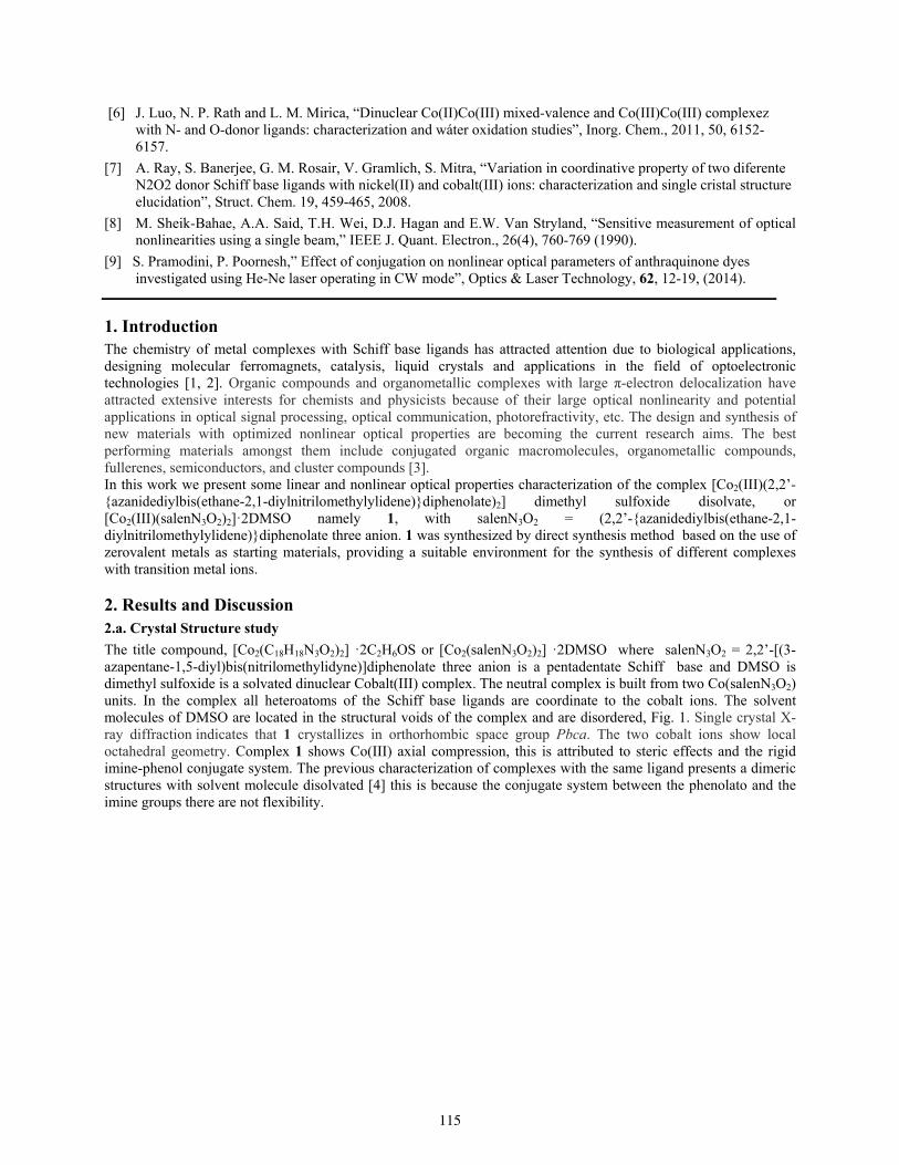
[6] J. Luo, N. P. Rath and L. M. Mirica, “Dinuclear Co(II)Co(III) mixed-valence and Co(III)Co(III) complexez with N- and O-donor ligands: characterization and wáter oxidation studies”, Inorg. Chem., 2011, 50, 6152-6157.

[7] A. Ray, S. Banerjee, G. M. Rosair, V. Gramlich, S. Mitra, “Variation in coordinative property of two diferente N2O2 donor Schiff base ligands with nickel(II) and cobalt(III) ions: characterization and single cristal structure elucidation”, Struct. Chem. 19, 459-465, 2008.

[8] M. Sheik-Bahae, A.A. Said, T.H. Wei, D.J. Hagan and E.W. Van Stryland, “Sensitive measurement of optical nonlinearities using a single beam,” IEEE J. Quant. Electron., 26(4), 760-769 (1990).

[9] S. Pramodini, P. Poornesh,” Effect of conjugation on nonlinear optical parameters of anthraquinone dyes investigated using He-Ne laser operating in CW mode”, Optics & Laser Technology, 62, 12-19, (2014).

1. Introduction The chemistry of metal complexes with Schiff base ligands has attracted attention due to biological applications, designing molecular ferromagnets, catalysis, liquid crystals and applications in the field of optoelectronic technologies [1, 2]. Organic compounds and organometallic complexes with large π-electron delocalization have attracted extensive interests for chemists and physicists because of their large optical nonlinearity and potential applications in optical signal processing, optical communication, photorefractivity, etc. The design and synthesis of new materials with optimized nonlinear optical properties are becoming the current research aims. The best performing materials amongst them include conjugated organic macromolecules, organometallic compounds, fullerenes, semiconductors, and cluster compounds [3]. In this work we present some linear and nonlinear optical properties characterization of the complex [Co2(III)(2,2’-{azanidediylbis(ethane-2,1-diylnitrilomethylylidene)}diphenolate)2] dimethyl sulfoxide disolvate, or [Co2(III)(salenN3O2)2]·2DMSO namely 1, with salenN3O2 = (2,2’-{azanidediylbis(ethane-2,1-diylnitrilomethylylidene)}diphenolate three anion. 1 was synthesized by direct synthesis method based on the use of zerovalent metals as starting materials, providing a suitable environment for the synthesis of different complexes with transition metal ions. 2. Results and Discussion 2.a. Crystal Structure study

The title compound, [Co2(C18H18N3O2)2] ·2C2H6OS or [Co2(salenN3O2)2] ·2DMSO where salenN3O2 = 2,2’-[(3-azapentane-1,5-diyl)bis(nitrilomethylidyne)]diphenolate three anion is a pentadentate Schiff base and DMSO is dimethyl sulfoxide is a solvated dinuclear Cobalt(III) complex. The neutral complex is built from two Co(salenN3O2) units. In the complex all heteroatoms of the Schiff base ligands are coordinate to the cobalt ions. The solvent molecules of DMSO are located in the structural voids of the complex and are disordered, Fig. 1. Single crystal X-ray diffraction indicates that 1 crystallizes in orthorhombic space group Pbca. The two cobalt ions show local octahedral geometry. Complex 1 shows Co(III) axial compression, this is attributed to steric effects and the rigid imine-phenol conjugate system. The previous characterization of complexes with the same ligand presents a dimeric structures with solvent molecule disolvated [4] this is because the conjugate system between the phenolato and the imine groups there are not flexibility.

115

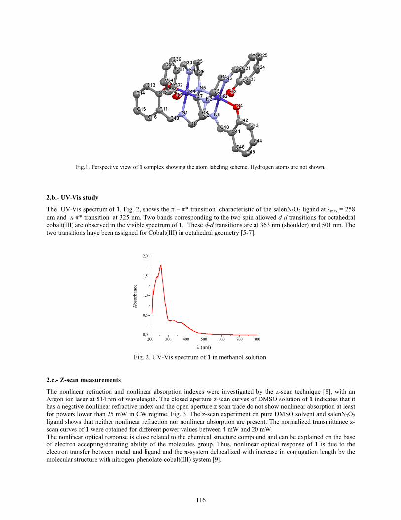
Fig.1. Perspective view of 1 complex showing the atom labeling scheme. Hydrogen atoms are not shown. 2.b.- UV-Vis study

The UV-Vis spectrum of 1, Fig. 2, shows the – * transition characteristic of the salenN3O2 ligand at λmax = 258 nm and n-* transition at 325 nm. Two bands corresponding to the two spin-allowed d-d transitions for octahedral cobalt(III) are observed in the visible spectrum of 1. These d-d transitions are at 363 nm (shoulder) and 501 nm. The two transitions have been assigned for Cobalt(III) in octahedral geometry [5-7].

200 300 400 500 600 700 8000,0

0,5

1,0

1,5

2,0

Abs

orba

nce

(nm) Fig. 2. UV-Vis spectrum of 1 in methanol solution.

2.c.- Z-scan measurements

The nonlinear refraction and nonlinear absorption indexes were investigated by the z-scan technique [8], with an Argon ion laser at 514 nm of wavelength. The closed aperture z-scan curves of DMSO solution of 1 indicates that it has a negative nonlinear refractive index and the open aperture z-scan trace do not show nonlinear absorption at least for powers lower than 25 mW in CW regime, Fig. 3. The z-scan experiment on pure DMSO solvent and salenN3O2 ligand shows that neither nonlinear refraction nor nonlinear absorption are present. The normalized transmittance z-scan curves of 1 were obtained for different power values between 4 mW and 20 mW. The nonlinear optical response is close related to the chemical structure compound and can be explained on the base of electron accepting/donating ability of the molecules group. Thus, nonlinear optical response of 1 is due to the electron transfer between metal and ligand and the π-system delocalized with increase in conjugation length by the molecular structure with nitrogen-phenolate-cobalt(III) system [9].

116

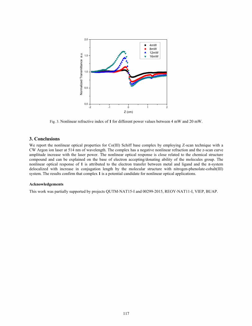
-2 -1 0 1 20,0

0,5

1,0

1,5

2,0

4mW 8mW 12mW 16mW

Nor

mal

ized

Tra

nsm

ittan

ce a

.u.

Z (cm)

Fig. 3. Nonlinear refractive index of 1 for different power values between 4 mW and 20 mW.

3. Conclusions We report the nonlinear optical properties for Co(III) Schiff base complex by employing Z-scan technique with a CW Argon ion laser at 514 nm of wavelength. The complex has a negative nonlinear refraction and the z-scan curve amplitude increase with the laser power. The nonlinear optical response is close related to the chemical structure compound and can be explained on the base of electron accepting/donating ability of the molecules group. The nonlinear optical response of 1 is attributed to the electron transfer between metal and ligand and the π-system delocalized with increase in conjugation length by the molecular structure with nitrogen-phenolate-cobalt(III) system. The results confirm that complex 1 is a potential candidate for nonlinear optical applications. Acknowledgements

This work was partially supported by projects QUTM-NAT15-I and 00299-2015, REOY-NAT11-I, VIEP, BUAP.

117

Coils and helical windings as polarization controllers

Diana Tentori, Alfonso García Weidner, and Miguel Farfán Sánchez

CICESE, División de Física Aplicada, Departamento de Óptica, México Corresponding author email: diana@cicese.mx

ABSTRACT:

Fiber coils have a wide application in fiber optics, since the necessity of compact fiber devices has been solved winding the fibers. However, coiled fibers show regularly a stress induced birefringence which needs to be taken into account. In general, it is only when two or three coils are combined that their polarization effects are not only considered relevant, but are used to control the state of polarization of light. These devices, known as polarization controllers, rely on the birefringence properties of the fiber coils and their relative orientation. The polarization performance of a three-ring polarization controller has been described assuming that the coil of each ring behaves as a quarter- or half-wave retarder [1]. This is a clear and useful approximation when the signal is monochromatic, but the verification of this assumption is not easy to accomplish.

In this work we verify the similar performance of polarization controllers built with two helical coils and with three non-regular windings, applying them to the cancellation of the effect of birefringence on the output state of polarization of a signal. We verify that states of polarization entering and leaving the controller can be equal using either option.

Key words: optical fiber; birefringence; polarization

REFERENCES AND LINKS [1] LeFevre, H. C. U.S. Patent No. 4,389,090. Washington, DC: U.S. Patent and Trademark Office. (1983).

[2] Tentori, D., Garcia Weidner, A., and Ledezma Sillas, E., "Birefringence description of a helical fiber coil" (submitted for publication).

[3] Tentori, D., García-Weidner, A., & Ayala-Díaz, C. "Birefringence matrix for a twisted single-mode fiber: Photoelastic and geometrical contributions." Optical Fiber Technology, 18, 14-20 (2012).

[4] Tentori, D., Ayala-Díaz, C., Treviño-Martínez, F., Mendieta-Jiménez, F. J., & Soto-Ortiz, H. "Birefringence evaluation of helically wound optical fibres." Journal of Modern Optics 48, 1767-1780 (2001).

[5] Tentori, D., Garcia Weidner, A., and Rodriguez Garcia, J. A., "Use of fiber helical coils to obtain polarization insensitive fiber devices" (submitted for publication).

[6] Rodriguez Garcia, J. A. (2013) "Cancelación del efecto de la birrefringencia residual en un multiplexor de bombeo 980/1550 nm de fibra óptica." Tesis de Maestría en Ciencias, CICESE. K. Lu y B. E. A. Saleh, “Theory and design of the liquid crystal TV as an optical spatial phase modulator”, Opt. Eng. 29, 240-246 (1990).

1. Introduction The necessity of compact fiber devices has been solved in practice using fiber coils. Nevertheless it is important to realize that when a fiber is coiled, its residual birefringence is modified. In general, it is only when two or three coils are combined that their polarization effects are considered relevant by the user. These devices, known as polarization

118

controllers (Fig. 1), rely on the birefringence properties of the fiber coils and their relative orientation. It should be noticed that even when only one fiber winding is used, strain-induced birefringence modifies the residual birefringence of the fiber and consequently the polarization performance of the fiber device. Comparing the polarization models reported in the literature for a helical fiber coil, we found there is no agreement on the descriptions presented by different authors. Since we consider it is important to understand these changes in order to build better fiber systems and devices, making use of the geometrical properties of a helix, we developed a birefringence model for a fiber helical coil. This matrix model includes the strain-induced birefringence of the helical coil (bend- and twist-induced) and the geometrical contribution due to its out-of-plane trajectory. Using the birefringence matrix model of one helical coil, we investigated the description of a polarization controller formed by two helical coils, taking into account the modification of the relative orientation of the separate fiber windings. We present an experimental comparison of polarization controllers formed by two helical coils and common polarization controllers using three non-regular coils, applying them to the cancellation of the effect of birefringence on the output state of polarization of a signal.

Fig.1.Polarizationcontrollerswiththreeandtwofiberrings.

2. Helical Fiber Structures 2.a.- Birefringence modification induced by helical windings

Making use of the geometrical properties of a helix, it has been recently shown [2] that a helical fiber coil, due to the residual elliptical birefringence of the uncoiled fiber (straight fiber), has linear and circular birefringence components. In addition, due to the helical winding, an additional linear birefringence (induced by bending) and a modification in the linear and circular components of the residual birefringence (produced by torsion) are observed [3]. Furthermore, since a helix is an out-of-plane curve, there is also a geometric rotation [4]. These results are important and explain why the comparison of the polarization models reported in the literature for a helical fiber show no agreement regarding their descriptions (references 4-22 in [2]).

Despite of all the phenomena involved, the resultant model is simple. It is equal to the product of a gyration matrix by an elliptical retarder matrix M with a twist dependence [2]

b R M , (1)

i.e., due to torsion, the retardation angle 0 between the polarization eigenmodes of the straight fiber is modified by a term that varies linearly with torsion ( = 0 + c, c is a constant), and the term b reflects the geometrical rotation of the fast birefringence axis (b is a constant) [3]; the gyration angle is equal to n2(1 - cos), being n the number of helix loops [4].

2.b.- Polarization controller formed by two helical coils

Two consecutive helical coils formed with fibers with equal length, radius and pitch length, but opposite handedness, allow the cancelation of the effect of birefringence on the state of polarization of the output signal (the

119

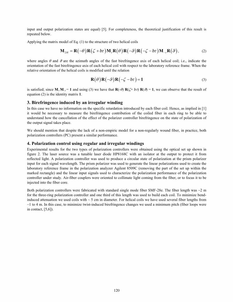
input and output polarization states are equal) [5]. For completeness, the theoretical justification of this result is repeated below.

Applying the matrix model of Eq. (1) to the structure of two helical coils

2H b b M R R M R R R M R , (2)

where angles and ϑ are the azimuth angles of the fast birefringence axis of each helical coil; i.e., indicate the orientation of the fast birefringence axis of each helical coil with respect to the laboratory reference frame. When the relative orientation of the helical coils is modified until the relation

b R R R 1 (3)

is satisfied; since M M- = 1 and using (3) we have that R(-) R(+ b) R(ϑ) = 1, we can observe that the result of equation (2) is the identity matrix 1.

3. Birefringence induced by an irregular winding In this case we have no information on the specific retardation introduced by each fiber coil. Hence, as implied in [1] it would be necessary to measure the birefringence contribution of the coiled fiber in each ring to be able to understand how the cancellation of the effect of the polarizer controller birefringence on the state of polarization of the output signal takes place.

We should mention that despite the lack of a non-empiric model for a non-regularly wound fiber, in practice, both polarization controllers (PC) present a similar performance.

4. Polarization control using regular and irregular windings Experimental results for the two types of polarization controllers were obtained using the optical set up shown in figure 2. The laser source was a tunable laser diode HP8168C with an isolator at the output to protect it from reflected light. A polarization controller was used to produce a circular state of polarization at the prism polarizer input for each signal wavelength. The prism polarizer was used to generate the linear polarizations used to create the laboratory reference frame in the polarization analyzer Agilent 8509C (removing the part of the set up within the marked rectangle) and the linear input signals used to characterize the polarization performance of the polarization controller under study. Air-fiber couplers were oriented to collimate light coming from the fiber, or to focus it to be injected into the fiber core.

Both polarization controllers were fabricated with standard single mode fiber SMF-28e. The fiber length was ~2 m for the three-ring polarization controller and one third of this length was used to build each coil. To minimize bend-induced attenuation we used coils with ~ 5 cm in diameter. For helical coils we have used several fiber lengths from ~1 to 4 m. In this case, to minimize twist-induced birefringence changes we used a minimum pitch (fiber loops were in contact, [5,6]).

120

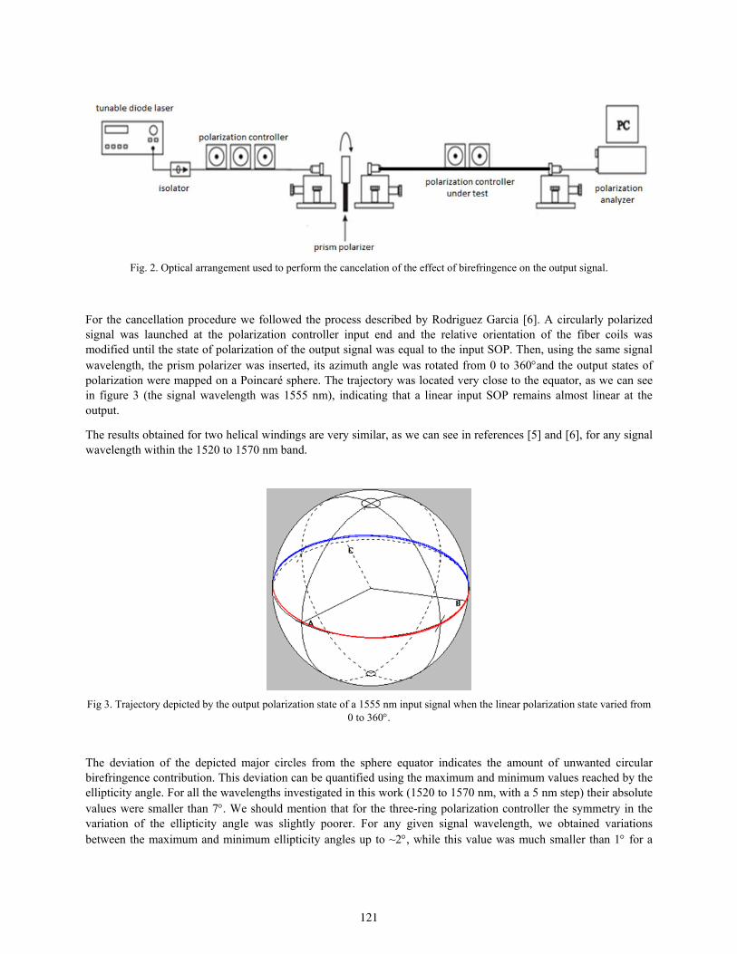
Fig. 2. Optical arrangement used to perform the cancelation of the effect of birefringence on the output signal.

For the cancellation procedure we followed the process described by Rodriguez Garcia [6]. A circularly polarized signal was launched at the polarization controller input end and the relative orientation of the fiber coils was modified until the state of polarization of the output signal was equal to the input SOP. Then, using the same signal wavelength, the prism polarizer was inserted, its azimuth angle was rotated from 0 to 360and the output states of polarization were mapped on a Poincaré sphere. The trajectory was located very close to the equator, as we can see in figure 3 (the signal wavelength was 1555 nm), indicating that a linear input SOP remains almost linear at the output.

The results obtained for two helical windings are very similar, as we can see in references [5] and [6], for any signal wavelength within the 1520 to 1570 nm band.

Fig 3. Trajectory depicted by the output polarization state of a 1555 nm input signal when the linear polarization state varied from 0 to 360.

The deviation of the depicted major circles from the sphere equator indicates the amount of unwanted circular birefringence contribution. This deviation can be quantified using the maximum and minimum values reached by the ellipticity angle. For all the wavelengths investigated in this work (1520 to 1570 nm, with a 5 nm step) their absolute values were smaller than 7. We should mention that for the three-ring polarization controller the symmetry in the variation of the ellipticity angle was slightly poorer. For any given signal wavelength, we obtained variations between the maximum and minimum ellipticity angles up to ~2, while this value was much smaller than 1 for a

121

system formed by two helical coils. These results showed only small variations of the maximum or minimum ellipticity angles (smaller than 2) within the 10 h time interval we monitored the stability of the output polarization states.

5. Conclusions The polarization control achieved by a polarization controller built with two helical coils of standard fiber is very similar to that achieved by a three-ring polarization controller built with non-regularly wound fiber coils for fiber lengths of ~ 2 to 3 m.

Acknowledgements

This work was sponsored by project SEP-CONACYT, SEP-CONACYT-CB-2010-155121.

122

Nonlocal Nonlinear Refraction of A(Acceptor)-π-D(Donor) Structures M.L. Arroyo Carrasco(1), I. Rincón Campeche(1), B.A. Martínez Irivas(1), M.M. Méndez Otero(1), M.D. Iturbe Castillo(2), J. Percino (3), V. Chapela (3), M. Cerón (3), G. Soriano (3), M.E. Castro (3)

1. Facultad de Ciencias Físico Matemáticas, BUAP, Av. San Claudio y 18 Sur, Col. San Manuel, C.P. 72570,

Puebla, Puebla, México. 2. Instituto Nacional de Astrofísica Óptica y Electrónica, Luis Enrique Erro #1, C.P. 72840, Tonantzintla,

Puebla, México. 3. Laboratorio de Polímeros, Centro de Química, ICUAP, BUAP, A.P. 1152, 72000. Puebla, Puebla, México.

Corresponding author email: marroyo@fcfm.buap.mx

ABSTRACT:

In this work the nonlinear refractive index of four α,β-unsatured acrylonitrile(π) with pyridine- (A) and dimethylaminophenyl-(D) moieties in methanol solution is measured with the z-scan technique. Z-scan is a widely used method because of their simplicity, accuracy and simple analysis. In order to explain experimental results many approaches to z-scan model have been developed, however, most of them based on a local spatial interaction between light and media. In reference [1], a z-scan model that takes into account the nonlocal character of the nonlinear interaction between a Gaussian beam and a thin medium has been proposed. The nonlocality of the interaction is labeled with an m parameter which describes the spatial extension of the photo-induced nonlinear phase shift at the output of the nonlinear medium; for m lower or higher than 2 the phase shift profile is bigger or smaller, respectively, than the input intensity profile, an m equal to 2 corresponds to the local case. In the base of this model we show that the presence of (CH3)2N-, -CN groups and the position of nitrogen atom in the pyridyl ring modify the z-scan amplitude curves and the nonlinear interaction nonlocality given different z-scan curve profiles reproduced with values of; 0.4, 2.0 and 4.0 for the m parameter. Key words: Nonlocal nonlinear interaction, z-scan, nonlinear refraction.

REFERENCES AND LINKS [1] E. V. Garcia Ramirez, M. L. Arroyo Carrasco, M. M. Mendez Otero, E. Reynoso Lara, S. Chavez-Cerda and M.

D. Iturbe Castillo, “Z-scan and spatial self-phase modulation of a Gaussian beam in a thin nonlocal nonlinear media,” J. Opt., 13, 085203(10pp) (2011).

[2] M. Sheik-Bahae, A.A. Said and E.W. Van Stryland, “High-sensitivity, single-beam n2 measurements,” Opt. Lett., 14(17), 955-957 (1989).

[3] M. Sheik-Bahae, A.A. Said, T.H. Wei, D.J. Hagan and E.W. Van Stryland, “Sensitive measurement of optical nonlinearities using a single beam,” IEEE J. Quant. Electron., 26(4), 760-769 (1990).

[4] D. Weaire, B.S. Wherrett, D.A.B. Miller and S.D. Smith, “Effect of low-power nonlinear refraction on laser-beam propagation in InSb,” Opt. Lett., 4(10), 331–333 (1979).

[5] S. Hughes, B. S. Wherrett, “Fast Fourier Transform techniques for efficient simulation of z-scan measurements,” J. Opt. Soc. Am. B, 12, 1888-1893 (1979).

[6] M.J. Percino, V.M. Chapela, M. Cerón, G. Soriano-Moro, M.E. Castro, F.J. Melendez, “Fluorescence improvement of pyridilacrylonitrile by dimethylaminophenyl-substitutions: the effect of packing modes of conjugated compounds,” J. Mol. Struc., 1034, 238-248 (2013)

123

1. Introduction The z-scan technique, proposed by Sheik-Bahae et al. [2, 3], is a widely used method to evaluate the nonlinear refraction, in the closed aperture configuration, and the nonlinear absorption, in the open aperture configuration. In this technique the on axis far field intensity is measured as function of the sample position. The transmittance after a thin sample that is illuminated by a Gaussian beam can be calculated with different methods like Gaussian decomposition (GD) [4], Fast Fourier Transform [5], etc. However in most of the cases only a local nonlinear response had been considered. In reference [1], a model to describe z-scan and spatial self-phase modulation of a Gaussian beam in a thin nonlocal nonlinear media that exhibits nonlinear refraction was presented. This model considers that the spatial extension of the photo-induced nonlinear phase shift at the output face of the sample can be bigger or smaller than the incident intensity profile on the input face of the sample. A Fast Fourier Transform algorithm is used, after the sample, to calculate the far field distribution and with this the on axis transmittance to obtain the z-scan curves. In this work using pyridilacrylonitrile molecules [6], we show that the presence of (CH3)2N-, -CN groups and the position of nitrogen atom in the pyridyl ring modify the nonlocality of the nonlinear interaction, giving as result different z-scan amplitude curves and profiles reproduced with three values of the m parameter. 2. Model

We consider a Gaussian beam propagating in the z direction with waist w0, wavelength , Rayleigh range z0=ω02/

and the following field amplitude:

2 2

00 2

( , ) exp exp ( )( ) 2 ( )( )

r rE r z A ikz ik i z

z R zz

(1)

where: A0 is a constant amplitude, k=2π/λ,1/22

0 0( ) 1 ( / )z z z the beam width, 20( ) 1 ( / )R z z z z the

radius of curvature of the wavefront and 10( ) tan ( / )z z z the Gouy phase retardation relative to a plane wave.

This beam is transmitted through a thin nonlinear optical media of length L<z0, with a refractive index coefficient given by [3]:

0( )n I n I , (2)

where: n0 is the linear refractive index, γ the nonlinear refractive coefficient and I the light intensity. The output field from a thin local media is given by;

riexpz,rEEout (3)

here it is considered that the sample absorption is negligible, z,rE is the incident field amplitude on the sample, r

the radial coordinate and the nonlinear phase change given by:

zmrexpm,zr 2

2

0 , (4)

where;

22

0

00

1m

zzm,z

, (5)

124

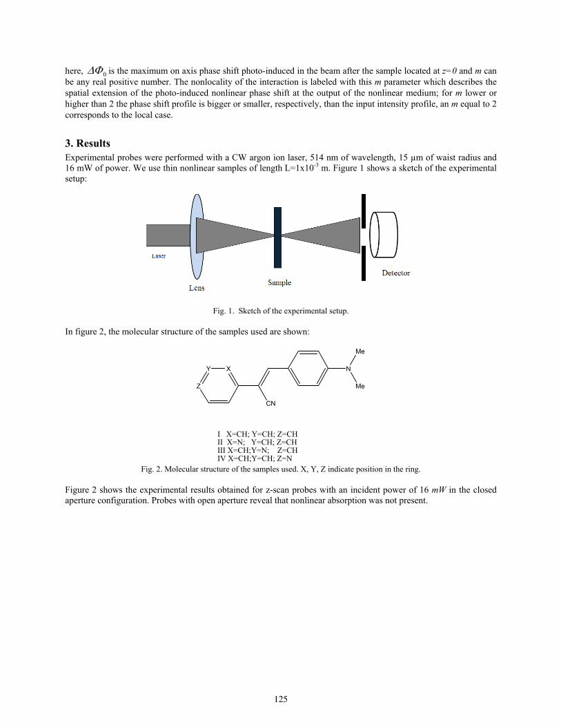
here, 0 is the maximum on axis phase shift photo-induced in the beam after the sample located at z=0 and m can be any real positive number. The nonlocality of the interaction is labeled with this m parameter which describes the spatial extension of the photo-induced nonlinear phase shift at the output of the nonlinear medium; for m lower or higher than 2 the phase shift profile is bigger or smaller, respectively, than the input intensity profile, an m equal to 2 corresponds to the local case.

3. Results Experimental probes were performed with a CW argon ion laser, 514 nm of wavelength, 15 µm of waist radius and 16 mW of power. We use thin nonlinear samples of length L=1x10-3 m. Figure 1 shows a sketch of the experimental setup:

Fig. 1. Sketch of the experimental setup. In figure 2, the molecular structure of the samples used are shown:

XY

Z

CN

N

Me

Me

I X=CH; Y=CH; Z=CHII X=N; Y=CH; Z=CHIII X=CH;Y=N; Z=CHIV X=CH;Y=CH; Z=N

Fig. 2. Molecular structure of the samples used. X, Y, Z indicate position in the ring. Figure 2 shows the experimental results obtained for z-scan probes with an incident power of 16 mW in the closed aperture configuration. Probes with open aperture reveal that nonlinear absorption was not present.

125

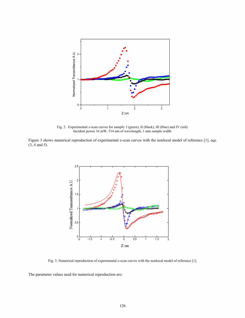
0 1 2 30

1

2

Nor

mal

ize

d T

rans

mitt

anc

e A

.U.

Z cm

Fig. 2. Experimental z-scan curves for sample: I (green), II (black), III (blue) and IV (red). Incident power 16 mW, 514 nm of wavelength, 1 mm sample width.

Figure 3 shows numerical reproduction of experimental z-scan curves with the nonlocal model of reference [1], eqs. (3, 4 and 5).

Fig. 3. Numerical reproduction of experimental z-scan curves with the nonlocal model of reference [1]. The parameter values used for numerical reproduction are:

126

TABLE I

Parameter values from numerical reproduction

Sample 0 rad m I -- -- II 0.84 2.0 III 3.36 4.0 IV 4.16 0.4

Theoretical calculations of static ( = 0.0) and dynamic ( = 3.67 x 1015 Hz), dipole polarizabilities and third-order hyper-polarizabilities were carried out using M06L/cc-pVDZ//6-311+G(d,p) theory level in Gaussian09 program in order to correlate with the compounds behavior, these are:

TABLE II

Theoretical dipole moment values

Dipolar Moment

(I) (II) (III) (IV)

x 4.7326 3.9636 -5.9870 8.3276 y -3.9833 -2.9612 -1.9768 -3.2335 z 0.3540 0.0341 -1.0679 0.1259 total 6.1959 4.9477 6.3947 8.9342

4. Conclusions In the base of this model we have shown that the presence of (CH3)2N-, -CN groups and the position of nitrogen atom in the pyridyl ring modify the z-scan amplitude curves and the nonlocality of the nonlinear interaction given different z-scan curve profiles reproduced with values of; 0.4, 2.0 and 4.0 for the m parameter. Theoretical calculations of dipole moments are in agreement with the z-scan amplitude curves.

Acknowledgements

This work was partially supported by project 00299-2015, VIEP, BUAP.

127

Optical Logic -AND- Gate Using a Nonlinear Discrete System

G. Mendoza-González(1) and Erwin A. Martí-Panameño(1,2)

1. Facultad de Ciencias Físico-Matemáticas, Benemérita Universidad Autónoma de Puebla. Av. San Claudio y 18

Sur, Col. San Manuel, Puebla 72570, México. 2. Laboratorio Nacional de Supercómputo del Sureste de México, Benemérita Universidad Autónoma de Puebla.

Blvd. Valsequillo y Av. Las Torres, Puebla 72570, México. http://www.lns.buap.mx Corresponding author email: gmendoza.glz@gmail.com

ABSTRACT:

In this work we present numerical results regarding the possibility to control the output position of the light in one-dimensional discrete system, composed by parallel dielectric subwavelength waveguides of circular cross section. Applying the finite difference time domain method, we numerically solve the Maxwell's equations with real values for the constitutive relations. The behavior of an optical logic AND gate is the result of the dynamics of nonlinear propagation and interaction of two optical fields, directly controlled by the amplitude of the input beams and the nonlinear Kerr coefficient of the waveguides.

Key words: Discrete system, subwavelength waveguides (SWG), FDTD method, optical logic AND gate.

REFERENCES AND LINKS [1] D. N. Christodoulides and R. I. Joseph, “Discrete self-focusing in nonlinear arrays of coupled waveguides”, Opt. Lett. 13, 794-796 (1988).

[2] H. S. Eisenberg et al., “Diffraction management”, Phys. Rev. Lett. 85, 1863-1866 (2000).

[3] R. Morandotti et al., “Self-focusing and defocusing in waveguide arrays”, Phys. Rev. Lett. 86, 3296–3299 (2001).

[4] Y. Liu et al., “Subwavelength discrete solitons in nonlinear metamaterials”, Phys. Rev. Lett. 99, 153901 (2007).

[5] C. Zhigang et al, “Optical spatial solitons: historical overview and recent advances”, Rep. Prog. Phys. 75(086401), 21 (2012).

[6] M. Foster et al, “Optimal waveguide dimensions for nonlinear interactions”, Opt. Express 12, 2880–2887 (2004).

[7] M. A. Foster et al., “Nonlinear optics in photonic nanowires”, Opt. Express 16, 1300–1320 (2008).

[8] K. Yee, “Numerical solution of initial boundary value problems involving maxwell’s equations in isotropic media”, Antennas and Propagation, IEEE Transactions on, 14, 302–307 (1966).

[9] C. M. Reinke et al., “Nonlinear finite-difference time-domain method for the simulation of anisotropic, χ(2), and χ(3) optical effects”, J. Lightwave Technol. 24, 624 (2006).

[10] G. Mendoza-González, E. A. Martí-Panameño, “Light interaction and self-trapping in subwavelength dielectric waveguide arrays”. J. Nanophoton. 9(1), 093071 (2015).

[11] S. Kasap and P. Capper, Springer Handbook of Electronic and Photonic Materials: Part D-45, Springer Science+ Business Media, New York (2006).

128

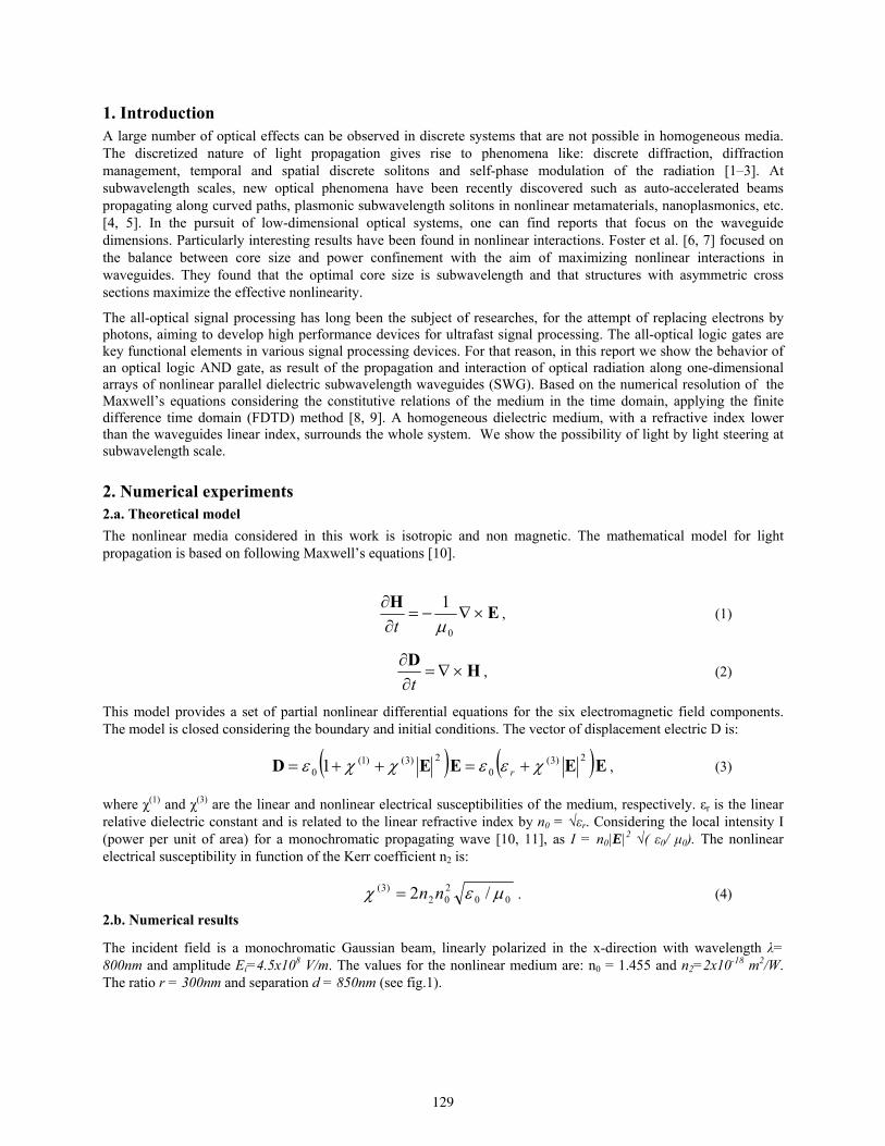
1. Introduction A large number of optical effects can be observed in discrete systems that are not possible in homogeneous media. The discretized nature of light propagation gives rise to phenomena like: discrete diffraction, diffraction management, temporal and spatial discrete solitons and self-phase modulation of the radiation [1–3]. At subwavelength scales, new optical phenomena have been recently discovered such as auto-accelerated beams propagating along curved paths, plasmonic subwavelength solitons in nonlinear metamaterials, nanoplasmonics, etc. [4, 5]. In the pursuit of low-dimensional optical systems, one can find reports that focus on the waveguide dimensions. Particularly interesting results have been found in nonlinear interactions. Foster et al. [6, 7] focused on the balance between core size and power confinement with the aim of maximizing nonlinear interactions in waveguides. They found that the optimal core size is subwavelength and that structures with asymmetric cross sections maximize the effective nonlinearity.

The all-optical signal processing has long been the subject of researches, for the attempt of replacing electrons by photons, aiming to develop high performance devices for ultrafast signal processing. The all-optical logic gates are key functional elements in various signal processing devices. For that reason, in this report we show the behavior of an optical logic AND gate, as result of the propagation and interaction of optical radiation along one-dimensional arrays of nonlinear parallel dielectric subwavelength waveguides (SWG). Based on the numerical resolution of the Maxwell’s equations considering the constitutive relations of the medium in the time domain, applying the finite difference time domain (FDTD) method [8, 9]. A homogeneous dielectric medium, with a refractive index lower than the waveguides linear index, surrounds the whole system. We show the possibility of light by light steering at subwavelength scale.

2. Numerical experiments 2.a. Theoretical model

The nonlinear media considered in this work is isotropic and non magnetic. The mathematical model for light propagation is based on following Maxwell’s equations [10].

EH

0

1

t, (1)

HD

t, (2)

This model provides a set of partial nonlinear differential equations for the six electromagnetic field components. The model is closed considering the boundary and initial conditions. The vector of displacement electric D is:

E EE ED2)3(

0

2)3()1(0 1 r , (3)

where χ(1) and χ(3) are the linear and nonlinear electrical susceptibilities of the medium, respectively. εr is the linear relative dielectric constant and is related to the linear refractive index by n0 = √εr. Considering the local intensity I (power per unit of area) for a monochromatic propagating wave [10, 11], as I = n0|E|2 √( ε0/ μ0). The nonlinear electrical susceptibility in function of the Kerr coefficient n2 is:

00202

)3( /2 nn . (4)

2.b. Numerical results

The incident field is a monochromatic Gaussian beam, linearly polarized in the x-direction with wavelength λ= 800nm and amplitude Ei=4.5x108 V/m. The values for the nonlinear medium are: n0 = 1.455 and n2=2x10-18 m2/W. The ratio r = 300nm and separation d = 850nm (see fig.1).

129

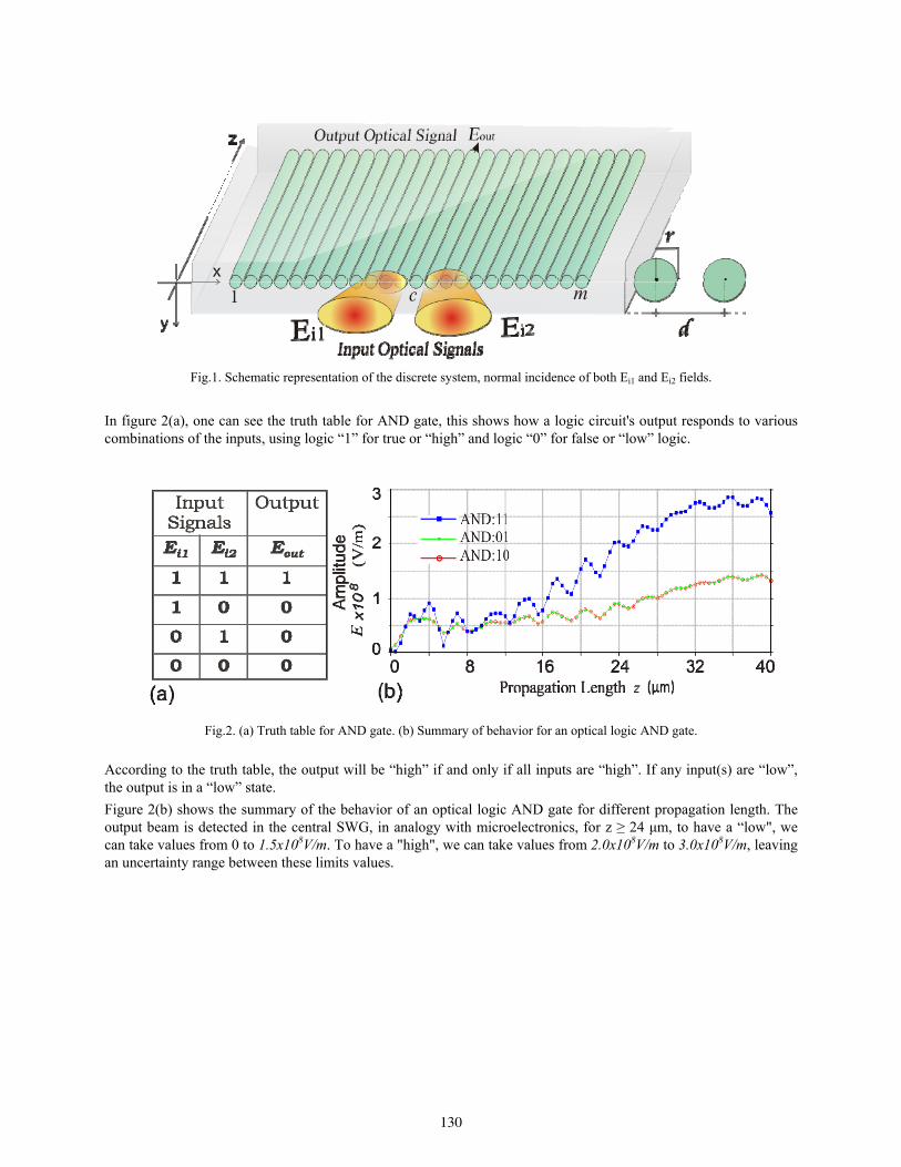
Fig.1. Schematic representation of the discrete system, normal incidence of both Ei1 and Ei2 fields.

In figure 2(a), one can see the truth table for AND gate, this shows how a logic circuit's output responds to various combinations of the inputs, using logic “1” for true or “high” and logic “0” for false or “low” logic.

Fig.2. (a) Truth table for AND gate. (b) Summary of behavior for an optical logic AND gate.

According to the truth table, the output will be “high” if and only if all inputs are “high”. If any input(s) are “low”, the output is in a “low” state.

Figure 2(b) shows the summary of the behavior of an optical logic AND gate for different propagation length. The output beam is detected in the central SWG, in analogy with microelectronics, for z ≥ 24 μm, to have a “low", we can take values from 0 to 1.5x108V/m. To have a "high", we can take values from 2.0x108V/m to 3.0x108V/m, leaving an uncertainty range between these limits values.

130

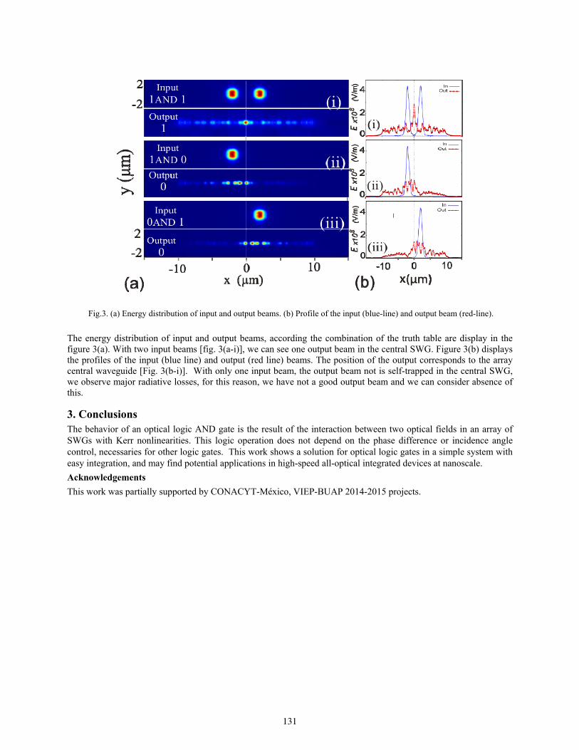
Fig.3. (a) Energy distribution of input and output beams. (b) Profile of the input (blue-line) and output beam (red-line).

The energy distribution of input and output beams, according the combination of the truth table are display in the figure 3(a). With two input beams [fig. 3(a-i)], we can see one output beam in the central SWG. Figure 3(b) displays the profiles of the input (blue line) and output (red line) beams. The position of the output corresponds to the array central waveguide [Fig. 3(b-i)]. With only one input beam, the output beam not is self-trapped in the central SWG, we observe major radiative losses, for this reason, we have not a good output beam and we can consider absence of this. 3. Conclusions The behavior of an optical logic AND gate is the result of the interaction between two optical fields in an array of SWGs with Kerr nonlinearities. This logic operation does not depend on the phase difference or incidence angle control, necessaries for other logic gates. This work shows a solution for optical logic gates in a simple system with easy integration, and may find potential applications in high-speed all-optical integrated devices at nanoscale.

Acknowledgements

This work was partially supported by CONACYT-México, VIEP-BUAP 2014-2015 projects.

131

Characterization of the fluorescence of colloidal ZnO nanoparticles obtained

at different ablation times

Luna Palacios Yryx Yanet (1,2,3,4), Camacho Lopez Marco Antonio (2), Camacho Lopez Miguel Angel (3), Aguilar Guillermo (4)

1.- Posgrado en Ciencia de Materiales, Facultad de Química, Universidad Autónoma del Estado

de México Paseo Colón y Tollocan, Toluca México, 50120, México 2. Laboratorio de Investigación y Desarrollo de Materiales Avanzados, Facultad de Química

Universidad Autónoma del Estado de México, Campus Rosedal, Km 14.5 Carretera TolucaAtlacomulco, San Cayetano de Morelos, C.P. 50925.

3. Laboratorio de Fotomedicina, Biofotónica y Espectroscopia Láser de Pulsos Ultracortos, Facultad de Medicina, Universidad Autónoma del Estado de México, Jesús Carranza y Paseo

Tollocan s/n. Toluca, México, C.P. 50120. 4. Department of Mechanical Engineering, University of California Riverside, 900 University

Ave., Bourns Hall A-341, Riverside, CA, USA. 92521.

Corresponding author email: yryxluna@gmail.com

ABSTRACT:

In the last decade, there has been interest on the synthesis and characterization of fluorescent colloidal Zinc Oxide Nanoparticles (ZnO NPs) due to its potential applications in biophotonics. Depending on the particle size and conditions of synthesis, ZnO NPs produce fluorescence at different wavelengths, going from blue through red in the visible spectrum. The Laser Ablation of Solids in Liquids (LASL) is a green technique that has been utilized to prepare metal, semiconductor and ceramic nanostructures. This method is experimentally simple and has been used to obtain metal oxides based colloidal solutions like ZnO. In this work we present results on the characterization of the fluorescence of colloidal ZnO NPs obtained by the LASL technique at different ablation times (10 - 60 min). The second harmonic of a nanosecond pulsed Nd-YAG laser (532 nm), a metallic Zinc disk and acetone were used to prepare the colloidal ZnO NPs. Samples were characterized by UV-Vis, fluorescence spectroscopy and TEM. Results show that the size and the optical properties of ZnO NPs are influenced by the ablation time, a blue emission (400-430 nm) is observed for samples obtained within an ablation time range of 10 - 30 min of ablation. A green emission (548 nm) is observed for samples obtained at 60 min of ablation

Key words: Zinc Oxide, Nanoparticles, fluorescence, Laser Ablation of Solids in Liquids and ablation time.

REFERENCES AND LINKS [1] P. Sharma, S. Brown, G. Walter, S. Santra, and B. Moudgil, “Nanoparticles for bioimaging”, Advances in Colloid and Interface Science, 123-126, 471–85 (2006). [2] B. E. Urban, P. Neogi, K. Senthilkumar, S. K. Rajpurohit, P. Jagadeeshwaran, Y. Fujita, and a. Neogi, “Bioimaging Using the Optimized Nonlinear Optical Properties of ZnO Nanoparticles,” IEEE J. Sel. Top. Quantum Electron. 18, 4, 1451–1456 (2012). [3] B. E. Urban, P. Neogi, Y. Fujita, and A. Neogi, “Colloidal ZnO nanoparticles for nonlinear optical probes and selective cell destruction,” Colloidal Nanocrystals for Biomedical Aplications. 8, 85950M (2013).

132

[4] L. Bonacina, “Nonlinear nanomedecine: harmonic nanoparticles toward targeted diagnosis and therapy”, Molecular Pharmaceutics, 10(3), 783–92 (2013). [5] Z. L. Wang , “ZnO Nanoparticles : Growth , Properties , and Applications”, Condens Matter. 16, R829-R858 (2004). [6] L. Irimpan, V.P.N Nampoori, P. Radhakrishnam, A. Deepthy and B. Krishnam “Size dependent fluorecence spectroscopy of nanocolloids of ZnO”, Applied Physics. 102, 063524 (2007). [7] D. Drranian and A. F. Eskandari “Effect of Laser Fluence on the Characteristics of ZnO Nanoparticles Produced by Laser Ablation in Acetone”, Mol. Cryst. Liq. Cryst. 607, 1-12 (2015). [8] J.M. Cho, J. K. Song and S. M. Park, “Characterization of ZnO Nanoparticles Grown by Laser Ablation of a Zn Target in Neat Water”, Bull. Korea Chem. Soc. 30 (7), 1616-1618 (2009). [9] S.C. Singh and R. Gopal, “Synthesis of coloidal zinc oxide nanoparticles by pulsed laser ablation in aqueous media”, Physica E. 40, 724-730 (2008). [10] K.K. Kim, D. Kim, S. K. Kim, S. M. Park and J. K. Song, “Formation of znO nanoparticles by laser ablation in neat water”, Chemical Physics Letters. 511, 116-120 (2011). [11] O. Khalid, “Investigation on Dielectric Constant of Zinc Oxide”, Modern Applied Science. 3(2), 110-116 (2009). [12] Y. T. Prabhu, K. V Rao, V. S. Sai Kumar and B. S. “Kumari, Synthesis of ZnO Nsnoparticles by Novel Surfactant Assisted Amine Combustion Method”, Advances in Nanoparticles. 2, 45-50 (2013).

1. Introduction Nanoparticles of zinc oxide (ZnO NPs) have become important because of their potential applications either in cosmetics, electrical devices, solar cells, in drug delivery [1], among others. On the other hand, the development and application of fluorescent biomarkers [2, 3], is very important because the optical bioimaging have helped us to understand various biological phenomena such as the identification of cells, realizing how it works; and sometimes in the delivery in vivo of drugs [1]. Currently, the markers used for obtaining these bioimages are the fluorochromes. However these markers have a shelf life of minutes, are expensive and emit a broadband spectrum [4]. Therefore new fluorescent materials such as quantum dots are an attractive option for generating those images [1]. Cadmium selenide (CdSe) and cadmium sulfide (CdS) quantum dots are two of the most important, however cadmium toxicity to the human body has been a concern.

On the other hand, ZnO NPs show low cytotoxicity than nanoparticles of CdSe or CdS. The ZnO has a bandgap of 3.37 eV and high bond energy (60 MeV) [5] making ZnO NPs very stable. Hence, it is unlikely to get different fluorescence emissions of ZnO NPs allowing us to have a wide range of dyes [6, 7], making it possible to detect different cell lines simultaneously. These emission wavelengths depend on the size of the nanoparticle and structural defects such as oxygen vacancies and interstitial zinc [6, 7, 8]. These defects and sizes of ZnO NPs can be regulated by the synthesis conditions [5, 6, 7, 8].

ZnO NPs are mostly synthesized by chemical synthesis [5]. However this method leads to obtain contaminated nanoparticles, generating problems when nanoparticles are intended to be functionalized [9].

Therefore, the use of novel methods to produce contaminant free nanoparticles in colloidal form, are essential for applications in biomedicine. One of such techniques is the Laser Ablation of Solids in Liquids (LASL), which consists of laser pulses impinge on a bulk material (target) immersed in a liquid medium. This method is experimentally simple and has been used to obtain metal oxides based colloidal solutions like ZnO.

We use the LASL for produce ZnO NPs at different ablation times (10 - 60 min) to observe the dependency of morphology and chemical structure according the ablation time increases.

2. Experiment and Results 2.a.- Experiment

ZnO NPs were produced by laser ablation of a Zn target (99.99%) placed at the bottom of a glass vessel filled with 10 ml of acetone. The Zn target was irradiated vertically at different ablation times (10 - 60 min) by the second harmonic (532 nm) of a nanosecond pulsed Nd-YAG laser operating at 15 Hz and with an energy of 25 mJ /pulse.

133

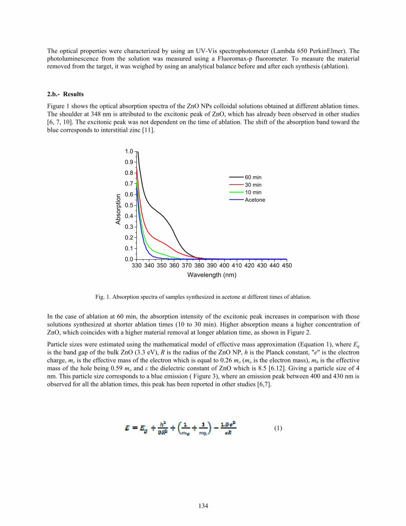
The optical properties were characterized by using an UV-Vis spectrophotometer (Lambda 650 PerkinElmer). The photoluminescence from the solution was measured using a Fluoromax-p fluorometer. To measure the material removed from the target, it was weighed by using an analytical balance before and after each synthesis (ablation).

2.b.- Results

Figure 1 shows the optical absorption spectra of the ZnO NPs colloidal solutions obtained at different ablation times. The shoulder at 348 nm is attributed to the excitonic peak of ZnO, which has already been observed in other studies [6, 7, 10]. The excitonic peak was not dependent on the time of ablation. The shift of the absorption band toward the blue corresponds to interstitial zinc [11].

330 340 350 360 370 380 390 400 410 420 430 440 4500.0

0.1

0.2

0.3

0.4

0.5

0.6

0.7

0.8

0.9

1.0

60 min 30 min 10 min Acetone

Abs

orp

tion

Wavelength (nm)

Fig. 1. Absorption spectra of samples synthesized in acetone at different times of ablation.

In the case of ablation at 60 min, the absorption intensity of the excitonic peak increases in comparison with those solutions synthesized at shorter ablation times (10 to 30 min). Higher absorption means a higher concentration of ZnO, which coincides with a higher material removal at longer ablation time, as shown in Figure 2.

Particle sizes were estimated using the mathematical model of effective mass approximation (Equation 1), where Eg is the band gap of the bulk ZnO (3.3 eV), R is the radius of the ZnO NP, h is the Planck constant, "e" is the electron charge, me is the effective mass of the electron which is equal to 0.26 mo (mo is the electron mass), mh is the effective mass of the hole being 0.59 mo and ε the dielectric constant of ZnO which is 8.5 [6.12]. Giving a particle size of 4 nm. This particle size corresponds to a blue emission ( Figure 3), where an emission peak between 400 and 430 nm is observed for all the ablation times, this peak has been reported in other studies [6,7].

(1)

134

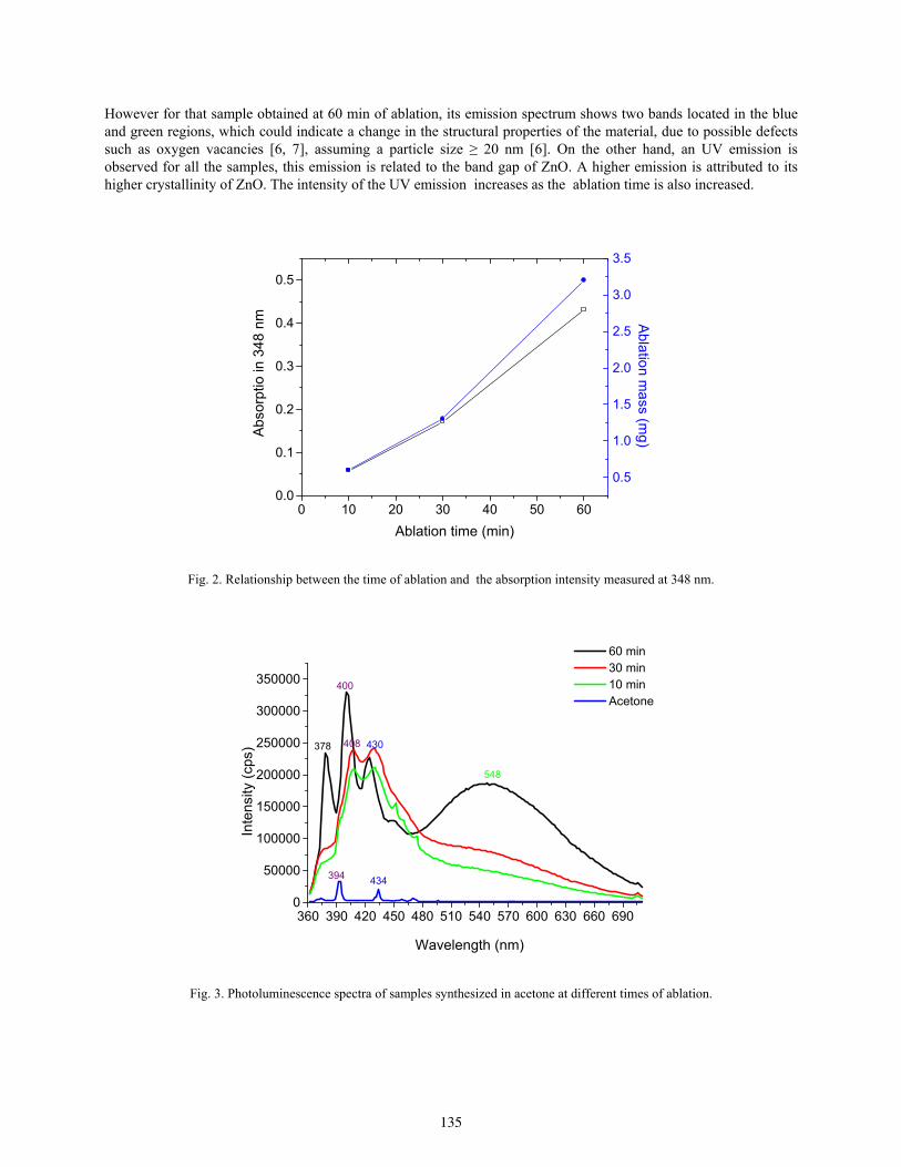
However for that sample obtained at 60 min of ablation, its emission spectrum shows two bands located in the blue and green regions, which could indicate a change in the structural properties of the material, due to possible defects such as oxygen vacancies [6, 7], assuming a particle size ≥ 20 nm [6]. On the other hand, an UV emission is observed for all the samples, this emission is related to the band gap of ZnO. A higher emission is attributed to its higher crystallinity of ZnO. The intensity of the UV emission increases as the ablation time is also increased.

0 10 20 30 40 50 600.0

0.1

0.2

0.3

0.4

0.5

Ablation time (min)

Abs

orpt

io in

348

nm

0.5

1.0

1.5

2.0

2.5

3.0

3.5A

blation m

ass (m

g)

Fig. 2. Relationship between the time of ablation and the absorption intensity measured at 348 nm.

360 390 420 450 480 510 540 570 600 630 660 6900

50000

100000

150000

200000

250000

300000

350000

434394

548

430408

400

378

60 min 30 min 10 min Acetone

Inte

nsi

ty (

cps)

Wavelength (nm)

Fig. 3. Photoluminescence spectra of samples synthesized in acetone at different times of ablation.

135

3. Conclusions It has been observed that varying the time of ablation it is possible to modify those parameters such as the particle size and its structural defects. This can be observed in the change of emission spectrum of each solution. Samples obtaining at 60 min of ablation time, show two emissions bands (blue and green). Therefore, the ablation time is seemed to be the critical parameter that allows to modify and control the optical properties of ZnO NPs.

Acknowledgements

Yryx Luna Palacios acknowledges to the CONACYT for financial support to developed her PhD studies. This work was partially supported by SIEA-UAEM under the contract 3798/2014/CID.

136

Optically obtained Bi2O3 thin films and its dependence on the per pulse laser fluence

A. Reyes-Contreras (1),(2), M. Camacho-López (2), A. Esparza-García(3), Y.

Esqueda-Barrón(4), S. Camacho-López(4)

1. Posgrado en Ciencia de Materiales, Facultad de Química, Universidad Autónoma del Estado de México Paseo Colón y Tollocan, Toluca México, 50120, México

2. Laboratorio de Investigación y Desarrollo de Materiales Avanzados, Universidad Autónoma del Estado de México, Km 14.5 Carretera Toluca-Atlacomulco, 50925, México

3. Fotofísica y Películas Delgadas, Departamento de Tecnociencias, CCADET-UNAM, Circuito exterior s/n C.P. 04510 Cd. Universitaria, D.F. México

4. Departamento de Óptica, Centro de Investigación Científica y de Educación Superior de Ensenada, Carretera Ensenada-Tijuana 3918, Zona Playitas, Ensenada, Baja California, 22860, México

Corresponding author email: adellerc@gmail.com

ABSTRACT:

In this work, we present results about of bismuth oxide formation on 500 nm thick bismuth film, using a Nd-YAG pulsed laser. A 532 nm laser wavelength with 9 ns pulse duration was incident on the sample to generate surface modifications on the bismuth films. Irradiated zones were characterized by scanning electron microscopy and micro-Raman spectroscopy. Results reveal that both the morphology and the oxidation degree inside the irradiation regions depend on the per pulse laser fluence. SEM shows the formation of unidimensional microstructures and micro-Raman shows that synthesis of the β-Bi2O3 phase was achieved.

Key words: bismuth oxide, thin films, laser pulses.

REFERENCES AND LINKS [1] A. J. Salazar-Pérez, M. A. Camacho-López, R. A. Morales-Luckie, V. Sánchez-Mendieta, “Structural evolution

of Bi2O3 prepared by thermal oxidation of bismuth nano-particles” Sup. y Vac. 18(3), 4-8 (2005).

[2] L. Kumari, J.-H. Lin and Y.-R. Ma, “Synthesis of bismuth oxide nanostructures by an oxidative metal vapour phase deposition technique” Nanotechnology 18 295605 (2007)

[3] L. Kumari, J.-H. Lin and Y.-R. Ma, “Laser oxidation and wide-band photoluminescence of thermal evaporated bismuth thin films”. J. Phys. D: Appl. Phys. 41 025405 (2008).

[4] K. S. Wu, M. Y. Chern, “Temperature-dependent growth of pulsed-laser-deposited bismuth thin films on glass substrates” Thin Solid Films 516 3808–3812 (2008).

[5] M. A. Zepeda, M. Picquart, and E. Haro-Poniatowski, “Laser Induced Oxidation Effects in Bismuth Thin Films” Mater. Res. Soc. Symp. Proc. 1477 (2012)

[6] A. Reyes. “Formación de estructuras periódicas inducidas por láser en películas delgadas de bismuto” Tesis licenciatura. Universidad Autónoma del Estado de México. (2015)

137

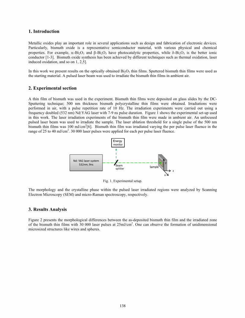
1. Introduction

Metallic oxides play an important role in several applications such as design and fabrication of electronic devices. Particularly, bismuth oxide is a representative semiconductor material, with various physical and chemical properties. For example, -Bi2O3 and -Bi2O3 have photocatalytic properties, while -Bi2O3 is the better ionic conductor [1-3]. Bismuth oxide synthesis has been achieved by different techniques such as thermal oxidation, laser induced oxidation, and so on 1, 2,5]. In this work we present results on the optically obtained Bi2O3 thin films. Sputtered bismuth thin films were used as the starting material. A pulsed laser beam was used to irradiate the bismuth thin films in ambient air.

2. Experimental section A thin film of bismuth was used in the experiment. Bismuth thin films were deposited on glass slides by the DC-Sputtering technique; 500 nm thickness bismuth polycrystalline thin films were obtained. Irradiations were performed in air, with a pulse repetition rate of 10 Hz. The irradiation experiments were carried out using a frequency doubled (532 nm) Nd:YAG laser with 7-9 ns pulse duration. Figure 1 shows the experimental set-up used in this work. The laser irradiation experiments of the bismuth thin film were made in ambient air. An unfocused pulsed laser beam was used to irradiate the sample. The laser ablation threshold for a single pulse of the 500 nm bismuth thin films was 100 mJ/cm2[6]. Bismuth thin film was irradiated varying the per pulse laser fluence in the range of 25 to 40 mJ/cm2. 30 000 laser pulses were applied for each per pulse laser fluence.

Fig. 1. Experimental setup.

The morphology and the crystalline phase within the pulsed laser irradiated regions were analyzed by Scanning Electron Microscopy (SEM) and micro-Raman spectroscopy, respectively.

3. Results Analysis Figure 2 presents the morphological differences between the as-deposited bismuth thin film and the irradiated zone of the bismuth thin films with 30 000 laser pulses at 25mJ/cm2. One can observe the formation of unidimensional microsized structures like wires and spheres.

138

Fig.2. SEM images (a) for the as-deposited bismuth thin film and (b) laser irradiated zone with 30000 pulses at 25 mJ/cm2 of a bismuth thin film

A Raman spectrum corresponding to the center of the laser irradiated region can be seen in Figure 3. The Raman bands are located at 314 and 464 cm-1 indicate the presence β-Bi2O3 [1-3, 5].

Fig. 3. Raman spectrum of Bi thin film taken at the center of the pulsed laser irradiated region.

4. Conclusions

We demonstrate that it is possible to induce oxidation on bismuth thin films at low per pulse laser fluence. Morphological changes were observed after the irradiation by nanosecond laser pulses on bismuth thin films. SEM images reveal that the laser irradiated material is constituted by microsized wires and spheres. Raman result showed that the irradiated material crystallized in the β-Bi2O3 phase. Acknowledgements

The authors acknowledge to Dr. Oscar Olea Mejía (Centro Conjunto en Química Sustentable-UAEMex) the Scanning Electron Microscopy Images.

139

Acousto-optic Interaction in Biconical Tapered Fibers: Broadening of the Stopbands

G. Ramírez-Meléndez (1)*, M. Bello-Jiménez (1), Balderas-Navarro R.(1), A. Rodríguez-Cobos(1),

G. Ramírez-Flores(1) R.),A. Diez(2), J.L. Cruz(2),M.V. Andrés(2)

1. Instituto de Investigación en Comunicación Óptica (IICO), Universidad Autónoma de San Luis Potosí, SLP 78210 México

2. Departamento de Física Aplicada y Electromagnetismo ICMUV, Universidad de Valencia. C/Dr.Moliner 50, Burjassot, Spain

*Corresponding author email: gustavo_r_melendez@hotmail.com

ABSTRACT:

We present an experimental and theoretical study of the acousto-optic interaction in biconical tapered fibers. For an acousto-optic filter, we show that it is possible to broaden the attenuation bandwidth as a consequence of the gradual reduction of the fiber diameter. The results of the experiments in tapered fibers with waist diameters of 90, 80, and 70 μm are compared with the developed theoretical model. For the fiber with waist diameter of 70 μm , it is demonstrated that the best spectral response is result not only of the contribution of the waist but also of the contribution of to the taper transitions. Optical bandwidth up to 45 nm is reported in a tapered fiber with a gradual reduction of the fiber down to 70μm diameter. Key words: acousto-optic interaction, biconical tapered fiber, acousto-optic filter

REFERENCES AND LINKS [1] R. Feced, C. Alegria, M.N. Zervas, and R.L. Laming, “Acousto-optic attenuation filters based on tapered

optical fibers”, IEEE J. Sel. Topics Quantum Electron. 5, 1278-1288 (1999) [2] T. A. Birks, P. St. Russel, and D. O. Culverhouse, “The acousto-optic effect in single mode fiber tapers and

couplers”, J. Ligthw. Technol. 14, 2519-2529 (1996)

[3] Q. Li, X. Liu, J. Peng, B. Zhou, E.R. Lyons, and H.P. Lee, “Highly efficient acousto-optic tunable filter based on cladding etched single mode fiber”, IEEE Photonic Technol . Letters, 14, 337-339 (2002)

[4] Okamoto K., Fundamentals of Optical Waveguides, London, England, Ed. Elsevier 2006

[5] C. Cuadrado Laborde, A. Díez, M.V. Andrés, J.L. Cruz, M. Bello Jimenez, I.L. Villegas, A. Martínez Gamez, and Y.O. Barkmenov. “Applications of in-fiber acousto-optic devices”, in the book “Acoustic waves- from Microdevices to Helioseismology”, InTech (2011)

1. Introduction It has been reported that the use of tapered fibers produces an enhancement in the response of acousto-optic attenuation filters [1]. This device is based on the phenomena of intermodal coupling that is produced by an flexural acoustic wave travelling along an uncoated region of the fiber. By reducing the diameter of the fiber the acoustic wave is focused in a smaller area and the overlap between modes is bigger [2]. Thus, the use of thin fibers produces a more efficient intermodal coupling that enables shorter and faster devices, as well as a reduction of the required acoustic power.

140

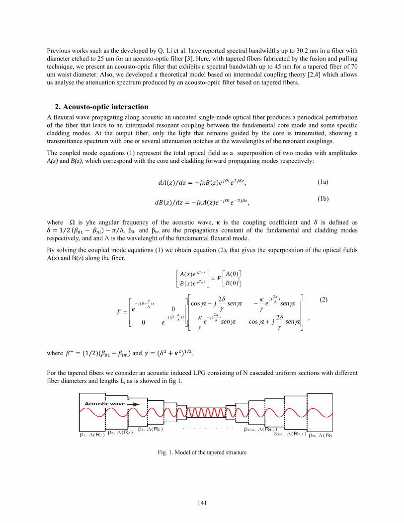
Previous works such as the developed by Q. Li et al. have reported spectral bandwidths up to 30.2 nm in a fiber with diameter etched to 25 um for an acousto-optic filter [3]. Here, with tapered fibers fabricated by the fusion and pulling technique, we present an acousto-optic filter that exhibits a spectral bandwidth up to 45 nm for a tapered fiber of 70 um waist diameter. Also, we developed a theoretical model based on intermodal coupling theory [2,4] which allows us analyse the attenuation spectrum produced by an acousto-optic filter based on tapered fibers.

2. Acousto-optic interaction A flexural wave propagating along acoustic an uncoated single-mode optical fiber produces a periodical perturbation of the fiber that leads to an intermodal resonant coupling between the fundamental core mode and some specific cladding modes. At the output fiber, only the light that remains guided by the core is transmitted, showing a transmittance spectrum with one or several attenuation notches at the wavelengths of the resonant couplings.

The coupled mode equations (1) represent the total optical field as a superposition of two modes with amplitudes A(z) and B(z), which correspond with the core and cladding forward propagating modes respectively:

⁄ ,

⁄ ,

where Ω is yhe angular frequency of the acoustic wave, κ is the coupling coefficient and is defined as 1 2⁄ Λ⁄ . β01 and βlm are the propagations constant of the fundamental and cladding modes

respectively, and and Λ is the wavelenght of the fundamental flexural mode.

By solving the coupled mode equations (1) we obtain equation (2), that gives the superposition of the optical fields A(z) and B(z) along the fiber.

,

where 1/2 and / .

For the tapered fibers we consider an acoustic induced LPG consisting of N cascaded uniform sections with different fiber diameters and lengths Li as is showed in fig 1.

Fig. 1. Model of the tapered structure

)0(

)0(

)(

)( 01

B

AF

ezB

ezAzj

zj

nl

zsenjzzsene

zsenezsenjz

e

eFj

j

zj

zj

2cos

2cos

0

0)

2(

)2

(

)(

)(

_

_

(1a)

(2)

(1b)

141

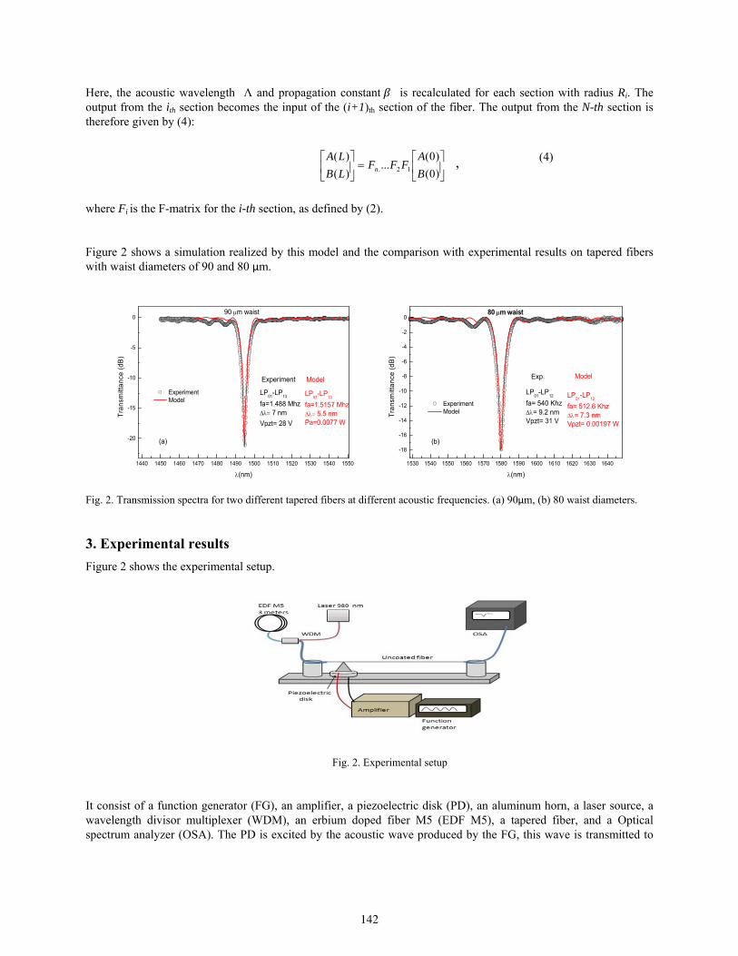
Here, the acoustic wavelength Λ and propagation constant is recalculated for each section with radius Ri. The output from the ith section becomes the input of the (i+1)th section of the fiber. The output from the N-th section is therefore given by (4):

where Fi is the F-matrix for the i-th section, as defined by (2).

Figure 2 shows a simulation realized by this model and the comparison with experimental results on tapered fibers with waist diameters of 90 and 80 μm.

Fig. 2. Transmission spectra for two different tapered fibers at different acoustic frequencies. (a) 90μm, (b) 80 waist diameters.

3. Experimental results

Figure 2 shows the experimental setup.

Fig. 2. Experimental setup

It consist of a function generator (FG), an amplifier, a piezoelectric disk (PD), an aluminum horn, a laser source, a wavelength divisor multiplexer (WDM), an erbium doped fiber M5 (EDF M5), a tapered fiber, and a Optical spectrum analyzer (OSA). The PD is excited by the acoustic wave produced by the FG, this wave is transmitted to

)0(

)0(...

)(

)(12. B

AFFF

LB

LAn

1440 1450 1460 1470 1480 1490 1500 1510 1520 1530 1540 1550

-20

-15

-10

-5

0

Model

LP01

-LP13

fa=1.5157 Mhz 5.5 nm Pa=0.0077 W

Experiment Model

Tra

nsm

itta

nce

(dB

)

(nm)

LP01

-LP13

fa=1.488 Mhz 7 nm

Vpzt= 28 V

Experiment

(a)

90 m waist

1530 1540 1550 1560 1570 1580 1590 1600 1610 1620 1630 1640

-18

-16

-14

-12

-10

-8

-6

-4

-2

0

Model

LP01

-LP12

fa= 512.6 Khz= 7.3 nmVpzt= 0.00197 W

Experiment ModelT

rans

mitt

anc

e (

dB)

(nm)

80 m waist

LP01

-LP12

fa= 540 Khz= 9.2 nmVpzt= 31 V

Exp.

(b)

(4) ,

142

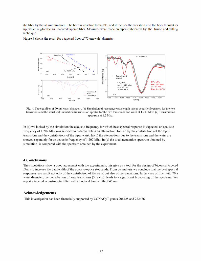
the fiber by the aluminium horn. The horn is attached to the PD, and it focuses the vibration into the fiber thought its tip, which is glued to an uncoated tapered fiber. Measures were made on tapers fabricated by the fusion and pulling technique

Figure 4 shows the result for a tapered fiber of 70 um waist diameter.

Fig. 4. Tapered fiber of 70 μm waist diameter . (a) Simulation of resonance wavelength versus acoustic frequency for the two transitions and the waist. (b) Simulation transmission spectra for the two transitions and waist at 1.207 Mhz. (c) Transmission

spectrum at 1.2 Mhz. In (a) we looked by the simulation the acoustic frequency for which best spectral response is expected, an acoustic frequency of 1.207 Mhz was selected in order to obtain an attenuation formed by the contributions of the taper transitions and the contributions of the taper waist. In (b) the attenuations due to the transitions and the waist are showed separately for an acoustic frequency of 1.207 Mhz. In (c) the total atenuattion spectrum obtained by simulation is compared with the spectrum obtained by the experiment.

4.Conclusions The simulations show a good agreement with the experiments, this give us a tool for the design of biconical tapered fibers to increase the bandwidth of the acousto-optics stopbands. From de analysis we conclude that the best spectral responses are result not only of the contribution of the waist but also of the transitions. In the case of fiber with 70 a waist diameter, the contribution of long transitions (5. 8 cm) leads to a significant broadening of the spectrum. We report a tapered acousto-optic filter with an optical bandwidth of 45 nm.

Acknowledgements

This investigation has been financially supported by CONACyT grants 206425 and 222476.

1480 1500 1520 1540 1560 1580 16001.18

1.20

1.22

1.24

1.26

transition 1 transition 2

Aco

ustic

fre

quen

cy (M

hz)

fa=1.207 Mhz

waist

(a)

1460 1480 1500 1520 1540 1560 1580 1600 1620

-6

-4

-2

0

LP01

-LP13

fa=1.1943 Mhz 45 nmVpzt= 44 V

LP01

-LP13

fa=1.207 Mhz51 nm

Pa= 9 x 10-3 W

Experiment Model

Tra

nsm

ittan

ce (dB

)

(nm)

70 m waist

(c)

1400 1450 1500 1550 1600 1650 1700-3

-2

-1

0

(nm)

Transition 1 Waist Transition 2

Tra

nsm

ittan

ce (dB

)

R(nm)

(b)

143

Numerical Analysis of Photonics Microstructures

Erick Ramón Baca Montero*, Pedro Pablo Rocha García, Oleksiy V. Shulika, José A. Andrade Lucio, Igor A. Sukhoivanov

Electronics Engineering Dept., DICIS, University of Guanajuato

*Email: er.bacamontero@ugto.mx ABSTRACT: Many applications require employment of a variety of ultrashort pulse waveforms. One of the key points in this analysis is the dispersion computation. The goal of this work is to analyse the dispersion properties of materials and use these properties to investigate the conditions for propagation and evolution of ultrashort optical pulses in structures for photonics applications (Mirrors, Gratings, Resonant Optical Structures). Characterization of materials by white light interferometry and the FDTD (Finite-Difference Time Domain) method is used. Subsequently it was implemented a one-dimensional FDTD simulation to model the propagation of ultrashort optical pulses in different photonics structures. Numerical simulations have been made and the characteristics (Reflectance, Phase, Group Delay, Group Delay Dispersion) obtained for these structures are analyzed, and to prove the accuracy and efficiency of our method above other alternatives we discuss the results in comparison to the characteristics obtained analytically by theories shown in the literature. Issues of resolution and convergence are discussed. Key words: Ultrashort Pulses, White-Light interferometry, FDTD, Bragg Mirror, Chirped Mirror, Dispersion

REFERENCES AND LINKS [1] N. Matuschek, F. X. Kärtner, U. Keller, “Theory of Double-Chirped Mirrors”, IEEE Journal of selected topics

in Quantum Electronics. Vol. 4, No. 2 (1998).

[2] S. O. Yakushev, I. A. Sukhoivanov, O. V. Shulika, V. V. Lysak, S. I. Petrov, “Modeling and Simulation of interaction of the ultrashort laser pulse with chirped mirror for structure design improvement”, Journal of Optoelectronics and Advanced Materials. Vol. 9, No. 8, 2384-2390 (2007).

[3] P. Hlubina, D. Ciprian, L. Knyblová, “Direct measurement of dispersion of the group refractive indices of quartz of crystal by white light spectral interferometry”, Optics Communications. 269, 8-13 (2007).

[4] D. B. Davidson, Computational Electromagnetics for RF and Microwave Engineering, Second Edition, Cambridge University Press (2010).

[5] A. Taflove & S. Hagness, Computational Electrodynamics: Finite Difference Time Domain Method, Third Edition, Norwood MA: Artech House (2005).

[6] N. Matuschek, F. X. Kärtner, U. Keller, “Exact coupled-mode theories for multilayer interference coatings with strong index modulations”, IEEE Journal of Quantum Electronics. Vol. 33, No. 3 (1997).

[7] R. C. Rumpf, “Improved Formulation of Scattering matrices for semi-analytical methods that is consistent with convention”, Progress in Electromagnetics Research B. Vol. 35, 241-261 (2011).

[8] W. H. Knox, N. M. Pearson, K. D. Li, C. A. Hirliman: Opt. Lett. 13, 574 (1988).

[9] C. Sáinz, P. Jourdain, R. Escalona, J. Calatroni, Optics Communications. 110 (1994).

[10] H. Delbarre, C. Przygodzki, M. Tassou, D. Boucher, Appl. Phys. B 70 45 (2000).

144

[11] J. Represa, C. Pereira, M. Panizo, F. Tadeo, “A simple demonstration of numerical dispersion under FDTD”, IEEE Transactions on Education. Vol. 40, 1, 98-102 (1997).

[12] D. E. Merewether, R. Fisher, F. W. Smith, “On implementing a numeric Huygen’s source scheme in a finite difference program to illuminate scattering bodies”, IEEE Trans. Nuclear Science. Vol. 27, 1829-1833 (1980).

1. Introduction Today ultrashort optical pulses have a huge range of applications due to their concentration of a large amount of energy within a short time interval and a broadband coherent pulse spectrum. Ultrashort optical pulses require high quality pulses, so dispersion becomes very important on this time scale [1, 2].

In this paper, it is proposed a White-light interferometry method based on the use of a white-light source in combination with a standard Michelson interferometer, as a tool to measure the refractive index dispersion for different optical materials. White-light interferometric methods enable high-accuracy measurements of group dispersion as well as higher-order dispersion of various optical elements over a broad spectral range [3]. Using Computational Electromagnetics, the process of modeling and simulating the interaction between electromagnetic fields and devices or structures is developed. In Computational Electromagnetics, many methods have been developed to model these interactions. Each method has its strength and weaknesses, as result the choice of a method is an important factor in solution of the problem [4].

A one-dimensional Finite Difference Time Domain (FDTD) based algorithm is implemented to be used widely in the modeling of propagation of ultrashort optical pulses in different photonics structures. Issues of resolution and convergence for implementation are discussed.

FDTD method is a Computational Electromagnetics technique to solve numerically the Maxwell equations by discretizing them in space and time, using centered finite differences [5]. Currently it is applied to the modeling of materials, waveguides, antenna design, wireless communications devices, multilayer circuit boards and bioelectromagnetic systems.

Subsequently, designs for Quarter-Wave Bragg Mirror [6] and Chirped Mirror [1] are analyzed numerically and the results discussed in comparison with others methods shown in literature as Exact coupled-mode theory [6] and Scattering Matrices [7]. Finally, it is presented the propagation of ultrashort pulses in a dispersive Debye medium.

2. Theory 2.a. White Light Interferometry for measurement of refractive index dispersion

White-light interferometry usually uses either of two methods, a temporal method or a spectral method, depending on whether interference is observed in the time domain or in the spectral domain, respectively [3].

A method for measuring the Group Delay (GD) introduced by an optical material consists in placing the sample in one arm of the interferometer and evaluating the temporal shift of the peak of the cross-correlation interferogram. As the central wavelength is varied, the relative GD of the frequency components is observed directly [8].

Alternatively, the spectral phase over the full bandwidth of the white light source can be obtained in a single measurement by a Fourier transform of the cross-correlation interferogram. The dispersion characteristics of the sample can be obtained by simply differentiating the measured spectral phase, as follows

GD( ) d()

d, (1)

The spectral method is based on the observation of spectrally resolved interference fringes (channeled spectrum) [9] and involves measurement of the period of the spectral fringes in the vicinity of a stationary-phase point [9] that

145

appears in the recorded spectral interferogram when the group optical path difference (OPD) between two beams in the interferometer is close to zero. The aim limitation of the method is reached for thick of strongly dispersive materials because under such condition the spectral interference fringes that are far from the stationary-phase point become difficult to solve. Fortunately, the measurement of the group refractive index dispersion of a given material is still possible in the vicinity of the stationary-phase point if one moves it in successive steps to different wavelengths [10] and repeats the measurement. The wavelengths are also referred to as the equalization wavelengths [10].

These effects can be well approximated to an analytical expression to describe the spectral dependence of the refractive index of a particular medium. Analytical dispersion models can be introduced in the FDTD method using Recursive-Convolution method or ADE-FDTD (Auxiliary Differential Equation) method [5].

2.b. FDTD method for photonics microstructures

FDTD method is based on discretizing the Maxwell’s curl equations

E

t

1

xH

e

E , (2)

H

t

1

xE

m

H , (3)

Where is the electric permittivity, e is the electric conductivity, is the magnetic permeability and m has no real meaning but allows to attenuate the magnetic field (a kind of artificial magnetic losses).

In [5], the rigorous finite difference derivation from equations (1) and (2) for one dimension in TE mode can be found

, (4)

, (5)

Herex is the grid space increment, called cell size, and t is the uniform time increment used during the observation interval. This is called shifted grid where the electric magnetic fields are calculated in terms of past fields until the observation interval is finished.

x resolution must be sufficient to resolve the shortest wavelength and the smallest mechanical feature of the structure to analyze.

In the FDTD grid, waves propagate slower than physical waves this arises as a consequence of the different phase and group velocities [11].t produces isotropic dispersion and, x grid resolution produces anisotropic dispersion. The principal effect is to push the spectral response to longer wavelengths. Increasing the grid resolution and decreasing the time increment can arbitrarily decrease numerical dispersion.

146

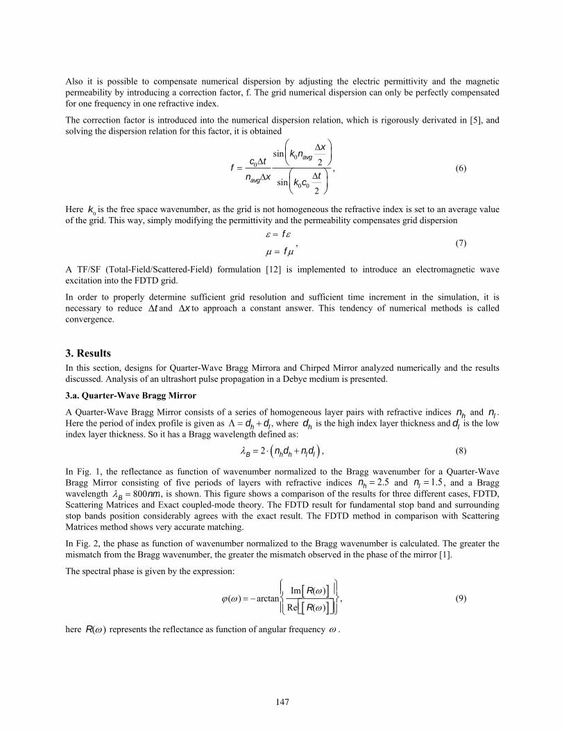
Also it is possible to compensate numerical dispersion by adjusting the electric permittivity and the magnetic permeability by introducing a correction factor, f. The grid numerical dispersion can only be perfectly compensated for one frequency in one refractive index.

The correction factor is introduced into the numerical dispersion relation, which is rigorously derivated in [5], and solving the dispersion relation for this factor, it is obtained

f c0t

navgx

sin k0navg

x

2

sin k0c0

t

2

, (6)

Here k0

is the free space wavenumber, as the grid is not homogeneous the refractive index is set to an average value of the grid. This way, simply modifying the permittivity and the permeability compensates grid dispersion

f

f, (7)

A TF/SF (Total-Field/Scattered-Field) formulation [12] is implemented to introduce an electromagnetic wave excitation into the FDTD grid.

In order to properly determine sufficient grid resolution and sufficient time increment in the simulation, it is necessary to reduce t and x to approach a constant answer. This tendency of numerical methods is called convergence.

3. Results In this section, designs for Quarter-Wave Bragg Mirrora and Chirped Mirror analyzed numerically and the results discussed. Analysis of an ultrashort pulse propagation in a Debye medium is presented.

3.a. Quarter-Wave Bragg Mirror

A Quarter-Wave Bragg Mirror consists of a series of homogeneous layer pairs with refractive indices nh and nl . Here the period of index profile is given as dh dl , where dh is the high index layer thickness and dl is the low index layer thickness. So it has a Bragg wavelength defined as:

B 2 nhdh nl dl , (8)

In Fig. 1, the reflectance as function of wavenumber normalized to the Bragg wavenumber for a Quarter-Wave Bragg Mirror consisting of five periods of layers with refractive indices and , and a Bragg wavelength , is shown. This figure shows a comparison of the results for three different cases, FDTD, Scattering Matrices and Exact coupled-mode theory. The FDTD result for fundamental stop band and surrounding stop bands position considerably agrees with the exact result. The FDTD method in comparison with Scattering Matrices method shows very accurate matching.

In Fig. 2, the phase as function of wavenumber normalized to the Bragg wavenumber is calculated. The greater the mismatch from the Bragg wavenumber, the greater the mismatch observed in the phase of the mirror [1].

The spectral phase is given by the expression:

( ) arctanIm R( )

Re R( )

, (9)

here R( ) represents the reflectance as function of angular frequency .

nh 2.5 nl 1.5B 800nm

147

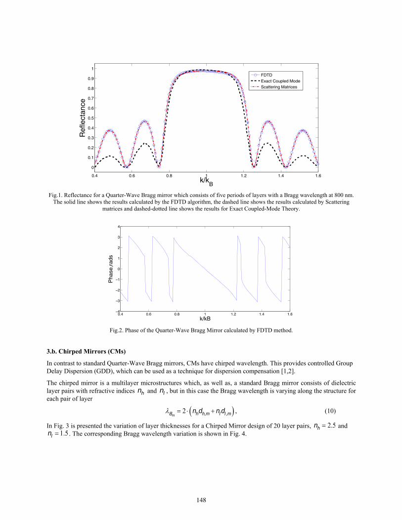
Fig.1. Reflectance for a Quarter-Wave Bragg mirror which consists of five periods of layers with a Bragg wavelength at 800 nm. The solid line shows the results calculated by the FDTD algorithm, the dashed line shows the results calculated by Scattering

matrices and dashed-dotted line shows the results for Exact Coupled-Mode Theory.

Fig.2. Phase of the Quarter-Wave Bragg Mirror calculated by FDTD method.

3.b. Chirped Mirrors (CMs)

In contrast to standard Quarter-Wave Bragg mirrors, CMs have chirped wavelength. This provides controlled Group Delay Dispersion (GDD), which can be used as a technique for dispersion compensation [1,2].

The chirped mirror is a multilayer microstructures which, as well as, a standard Bragg mirror consists of dielectric layer pairs with refractive indices and , but in this case the Bragg wavelength is varying along the structure for each pair of layer

Bm 2 nhdh,m nl dl ,m , (10)

In Fig. 3 is presented the variation of layer thicknesses for a Chirped Mirror design of 20 layer pairs, and . The corresponding Bragg wavelength variation is shown in Fig. 4.

0.4 0.6 0.8 1 1.2 1.4 1.6

0

0.1

0.2

0.3

0.4

0.5

0.6

0.7

0.8

0.9

1

k/kB

Ref

lect

ance

FDTDExact Coupled ModeScattering Matrices

nh nl

nh 2.5nl 1.5

148

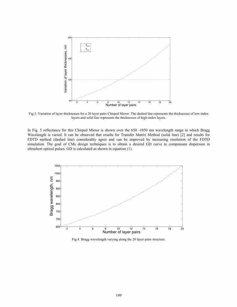
Fig.3. Variation of layer thicknesses for a 20 layer pairs Chirped Mirror. The dashed line represents the thicknesses of low-index layers and solid line represents the thicknesses of high-index layers.

In Fig. 5 reflectance for this Chirped Mirror is shown over the 650 -1050 nm wavelength range in which Bragg Wavelength is varied. It can be observed that results for Transfer Matrix Method (solid line) [2] and results for FDTD method (dashed line) considerably agree and can be improved by increasing resolution of the FDTD simulation. The goal of CMs design techniques is to obtain a desired GD curve to compensate dispersion in ultrashort optical pulses. GD is calculated as shown in equation (1).

Fig.4. Bragg wavelength varying along the 20 layer pairs structure.

2 4 6 8 10 12 14 16 18 2050

100

150

200

Number of layer pairs

Var

iatio

n of

laye

r th

ickn

esse

s, n

m

dh,m

dl,m

2 4 6 8 10 12 14 16 18 20650

700

750

800

850

900

950

1000

1050

Number of layer pairs

Bra

gg w

avel

engt

h, n

m

149

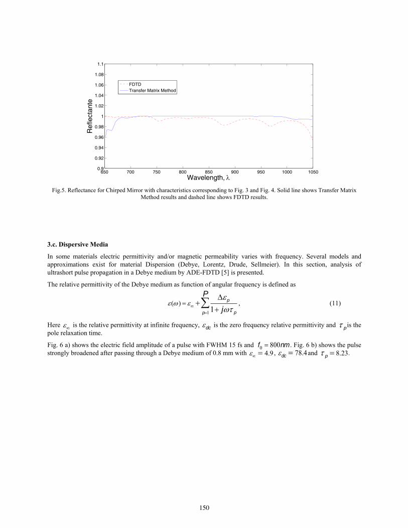
Fig.5. Reflectance for Chirped Mirror with characteristics corresponding to Fig. 3 and Fig. 4. Solid line shows Transfer Matrix Method results and dashed line shows FDTD results.

3.c. Dispersive Media

In some materials electric permittivity and/or magnetic permeability varies with frequency. Several models and approximations exist for material Dispersion (Debye, Lorentz, Drude, Sellmeier). In this section, analysis of ultrashort pulse propagation in a Debye medium by ADE-FDTD [5] is presented.

The relative permittivity of the Debye medium as function of angular frequency is defined as

( ) p

1 j pp1

P , (11)

Here is the relative permittivity at infinite frequency, dc is the zero frequency relative permittivity and pis the pole relaxation time.

Fig. 6 a) shows the electric field amplitude of a pulse with FWHM 15 fs and f0 800nm. Fig. 6 b) shows the pulse strongly broadened after passing through a Debye medium of 0.8 mm with 4.9, dc 78.4and p 8.23.

650 700 750 800 850 900 950 1000 10500.9

0.92

0.94

0.96

0.98

1

1.02

1.04

1.06

1.08

1.1

Wavelength,

Ref

lect

ante

FDTDTransfer Matrix Method

150

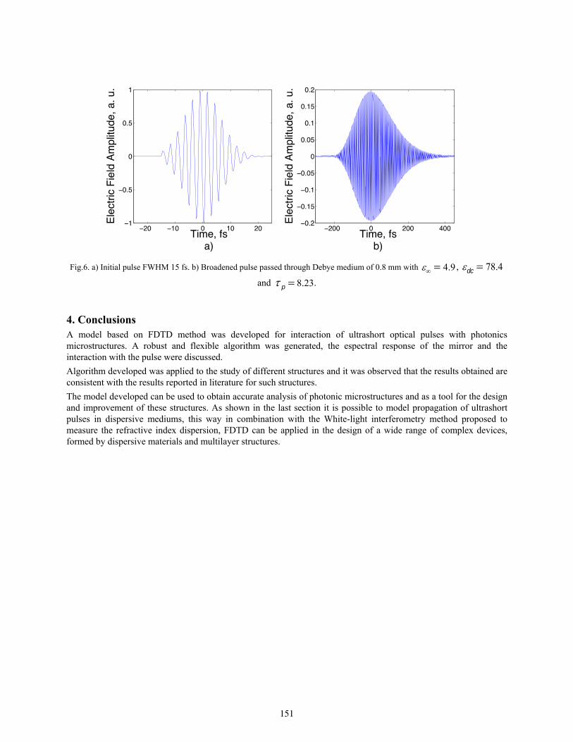
Fig.6. a) Initial pulse FWHM 15 fs. b) Broadened pulse passed through Debye medium of 0.8 mm with 4.9, dc 78.4

and p 8.23.

4. Conclusions A model based on FDTD method was developed for interaction of ultrashort optical pulses with photonics microstructures. A robust and flexible algorithm was generated, the espectral response of the mirror and the interaction with the pulse were discussed.

Algorithm developed was applied to the study of different structures and it was observed that the results obtained are consistent with the results reported in literature for such structures.

The model developed can be used to obtain accurate analysis of photonic microstructures and as a tool for the design and improvement of these structures. As shown in the last section it is possible to model propagation of ultrashort pulses in dispersive mediums, this way in combination with the White-light interferometry method proposed to measure the refractive index dispersion, FDTD can be applied in the design of a wide range of complex devices, formed by dispersive materials and multilayer structures.

151

Multiple photorefractive waveguides formed by diffraction effect Múltiples guías de onda fotorrefractivas formadas por efecto de difracción

J. A. Andrade-Lucio1, O. V. Shulika1*, D. F. Ortega –Tamayo1, I. V. Guryev2,

E. Alvarado-Méndez1, I. A. Sukhoivanov1

1. Departamento de Electrónica, DICIS, Universidad de Guanajuato, Salamanca, Gto., México 2. Departamento de estudios multidisciplinarios, DICIS, Universidad de Guanajuato, Yuriria, Gto., México

(*) E-mail: oshulika@ugto.mx

ABSTRACT: The richness of the nonlinear effects in photorefractive media has given rise to many theoretical and experimental studies in these materials. For example, soliton effects play a very important and exiting role in the formation of nonlinear wave fields in photorefractive crystals. In this work we study experimentally an interaction of a diffracted optical field with a photorefractive crystal. Self-formation of one-dimensional multiple waveguides is observed in a SBN photorefractive crystal under drift nonlinearity. Laser beam of only a few miliwatts diffracted on a straight edge is incident to SBN crystal and forms multiple steady-state patterns of the waveguides in a properly biased photorefractive crystal. Key words: Photorefractive materials, solitons, SBN crystal

REFERENCES AND LINKS [1] V. A. Vysloukh, V. Kutuzov, V. M. Petnikova, and V. V. Shuvalov, “Formation of spatial solitons and

spatial shock waves in photorefractive crystals.” JETP 84 (2), 338-394 (1997). [2] M. Segev, B. Crosignani, A. Yariv, and B. Fisher, “Spatial solitons in photorefractive media.” Phys. Rev.

Lett. 68, 923-926 (1992). [3] M. D. Iturbe-Castillo, P. A. Márquez-Aguilar, J. J. Sánchez-Mondragón, and S. Stepanov, “Spatial solitons

in photorefractive Bi12TiO20 with drift mechanism of nonlinearity” Appl. Phys. Lett. 64 (4), 408-410 (1994).

[4] G. Duree, J. Shultz, G. Salamo, et. al., “Observation of self-trapping of an optical beam due to the photorefractive effect” Phys. Rev. Lett., 71 (4), 533-536 (1993).

[5] P. Yeh, Introduction to photorefractive nonlinear optics. Wiley, New York (1993). [6] J. A. Andrade-Lucio, et. al., “Optical switching by coherent collision of spatial solitons” Electron. Lett. 36

(16), 14031405 (2000).

1. Introduction The photorefractive effect is a phenomenon in which the local index of refraction of a medium is changed by the illumination of a beam of light with spatial variation of the intensity [5]. The photorefractive beam dynamics are the result of the combined effect of optical wave propagation and the electro-optic response to the electric field generated by the displacement of photoexcited charge in the photorefractive crystal (PRC). In this sense, the photorefractive crystals offer unique characteristics: The optical response of the photorefractive effect is normally independent of the intensity and we can observe delayed effects, which make it possible to regulate the time for the formation of the nonlinear response from seconds to a milliseconds or less. The other one is the nonlocal nature of the photorefractive index grating, which is the origin of optical beam coupling in the PRC, this is the reason to use this effect in many applications related to photonics, including optical image processing, pattern recognition, parallel optical logic, and optical switching.

152

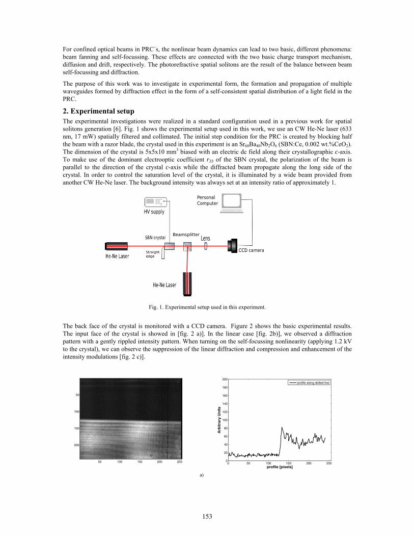
For confined optical beams in PRC´s, the nonlinear beam dynamics can lead to two basic, different phenomena: beam fanning and self-focussing. These effects are connected with the two basic charge transport mechanism, diffusion and drift, respectively. The photorefractive spatial solitons are the result of the balance between beam self-focussing and diffraction.

The purpose of this work was to investigate in experimental form, the formation and propagation of multiple waveguides formed by diffraction effect in the form of a self-consistent spatial distribution of a light field in the PRC.

2. Experimental setup The experimental investigations were realized in a standard configuration used in a previous work for spatial solitons generation [6]. Fig. 1 shows the experimental setup used in this work, we use an CW He-Ne laser (633 nm, 17 mW) spatially filtered and collimated. The initial step condition for the PRC is created by blocking half the beam with a razor blade, the crystal used in this experiment is an Sr60Ba40Nb2O6 (SBN:Ce, 0.002 wt.%CeO2). The dimension of the crystal is 5x5x10 mm3 biased with an electric dc field along their crystallographic c-axis. To make use of the dominant electrooptic coefficient r33 of the SBN crystal, the polarization of the beam is parallel to the direction of the crystal c-axis while the diffracted beam propagate along the long side of the crystal. In order to control the saturation level of the crystal, it is illuminated by a wide beam provided from another CW He-Ne laser. The background intensity was always set at an intensity ratio of approximately 1.

Fig. 1. Experimental setup used in this experiment.

The back face of the crystal is monitored with a CCD camera. Figure 2 shows the basic experimental results. The input face of the crystal is showed in [fig. 2 a)]. In the linear case [fig. 2b)], we observed a diffraction pattern with a gently rippled intensity pattern. When turning on the self-focussing nonlinearity (applying 1.2 kV to the crystal), we can observe the suppression of the linear diffraction and compression and enhancement of the intensity modulations [fig. 2 c)].

a)

50 100 150 200 250

50

100

150

200

0 50 100 150 200 2500

20

40

60

80

100

120

140

160

180

200

profile [pixels]

Arb

itra

ry U

nit

s

profile along dotted line

153

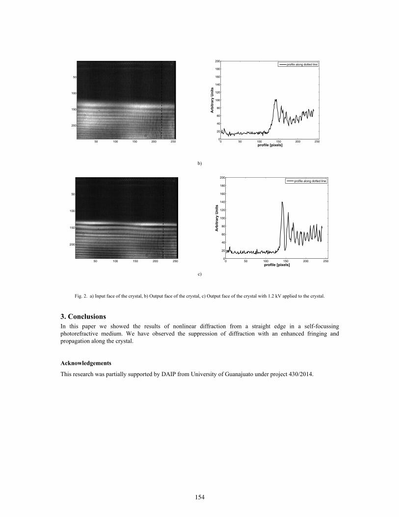
b)

c)

Fig. 2. a) Input face of the crystal, b) Output face of the crystal, c) Output face of the crystal with 1.2 kV applied to the crystal.

3. Conclusions In this paper we showed the results of nonlinear diffraction from a straight edge in a self-focussing photorefractive medium. We have observed the suppression of diffraction with an enhanced fringing and propagation along the crystal.

Acknowledgements

This research was partially supported by DAIP from University of Guanajuato under project 430/2014.

50 100 150 200 250

50

100

150

200

0 50 100 150 200 2500

20

40

60

80

100

120

140

160

180

200

profile [pixels]

Arb

itra

ry U

nit

s

profile along dotted line

50 100 150 200 250

50

100

150

200

0 50 100 150 200 2500

20

40

60

80

100

120

140

160

180

200

profile [pixels]

Arb

itra

ry U

nit

s

profile along dotted line

154

AUTHOR INDEX

A Acevedo Carrera: 41

Aguilar Guillermo: 132 Alanís Carranza L.E.: 90 Alcántara Flores J. L.: 114 Alvarado-Méndez E.: 152 Alvarez Herrera Cornelio: 12, 104 Álvarez-Borrego Josué: 19 Álvarez-Chávez J.A.: 90 Álvarez-Tamayo R.I.: 35 Andrade Lucio José A.: 144,152 Andrés M.V.: 140 Arceo Olague J.: 54 Arroyo Carrasco Maximino Luis: 99, 110, 114, 123

 

B Baca Montero Erick Ramón: 144 Balderas-Navarro R.E.: 140 Barajas-García Carolina: 19 Barbosa-García O.: 73 Barcelata-Pinzon A.: 35 Barojas Gutiérrez E.:35 Bello-Jiménez M.: 140 Berriel Valdos L.R.: 54

 

C Camacho López Marco Antonio 132 Camacho López Miguel Ángel: 132, 137 Camacho-López S.: 137 Carrasco-Valenzuela L.: 104

Castillo-Torres J.: 104 Castro M.E.: 123 Cerón M.: 123 Cisneros Martínez José Antonio: 12 Chapela V.: 123 Cruz J. L.: 140

 

D Dávila A.: 45 De la Rosa Miranda E.: 54 De la Rosa Vargas J. I.: 54 Desirena H.: 94 Diez A.: 140 Durán-Sánchez M.: 35

 

E Esparza-García A.: 137 Espinosa Luna Rafael:1 Esqueda-Barrón Y.: 137 Estrada Dorado S.: 41 Estudillo Ayala J. M.: 67

 

F Farfán Sánchez Miguel: 118 Frausto-Rea G.: 45

 

G Gallegos Alegría N.: 35 García Weidner Alfonso: 118 Gómez Vieyra Armando: 12, 90 Guryev I. V.: 152

HHernández Candia Carmen Noemí: 47 Herrera-Estévez J. A.: 90 Herrera G.: 104 Huerta Mascotee E. H.: 67

I Ibarra-Manzano O. G.: 152 Iturbe Castillo Marcelo David: 99, 110, 114, 123

J Jáuregui Vázquez D.:67 Juárez-Salazar R.: 35

L Lara Rodríguez Luis David: 27 Lazcano H. E.: 77 López Dieguez Y.: 67 López Meléndez Elizabeth: 27 López Morales Guadalupe: 1 Luna Palacios Yanet: 132

M Maldonado J. L.: 73 Martínez Irivas B.A.: 110, 123 Martí-Panameño Erwin A.: 128 Mcdonald R.: 114 Mejía Alanís Francisco Carlos: 6 Méndez Otero Marcela Maribel: 99, 110, 114, 123

155

Mendoza B. S.: 68 Mendoza-González Gregorio: 128 Mendoza-Suárez Alberto: 82 Meneses Marco Antonio: 73 Meneses-Fabian Cruz: 35 Molina J. A.: 94 Montenegro Orenday J. A.: 67 Moreno López F.: 41 Muñoz Rodríguez J. Apolinar: 6 Muñoz-Mata J. L.: 35 Murillo J. G.: 104

 

O Olvera Olvera C. A.: 54 Ortega-Tamayo D. F.: 152 Ortiz-Sosa R.: 51 Oskam Gerko: 15 Ostrovsky Andrey S.: 61

 

P Palacios L. R: 94 Percino J.: 123 Pérez Maciel M.: 67 Pérez-Aguilar Héctor: 82 Pérez-Sánchez G.G.: 90 Perez-Tiscareño A.: 94

 

Q Quintero Téllez M. G.: 114

 

R Ramírez-Flores G.: 140

Ramírez-Meléndez G.: 140 Ramos-Ortíz G.: 73 Renero Carrillo Francisco Javier: 27 Reyes Ortega Y.: 114 Reyes-Contreras A.: 137 Rincón Campeche I.: 123 Robledo-Sánchez C.: 35 Rocha García Pedro Pablo: 144 Rojas Laguna R.: 67 Rodríguez-Cobos A.: 140

Rosas-Roman I.: 73

 

S Sandoval- Romero G. E.: 90 Saucedo Anayac T.: 54 Saucedo Orozco Izcoatl:1 Shulika Oleksiy V.: 144, 152Sierra Hernández J. M.: 67 Solorza-Calderón Selene: 19 Soriano G.: 123 Sukhoivanov Igor A.: 144, 152

 

T Tentori Diana: 118 Torres Quiñonez L.: 41 Torres R. A.: 77 Torres Romero Roman: 99

 

U Urcid Gonzalo: 27

 

V

Vázquez G. V.: 77 Vega-Rios A.: 104 Vélez Juárez Esteban: 61

Z Zhan Qiwen:1

155

Z

Zalevsky Zeev: 6, 17 Zamarreño C. R.: 69 Zhan Qiwen: 29, 31 Zurita-Sánchez Jorge R.: 46