Process Capability for Large-Volume Production

8/11/2019 Process Capability for Large-Volume Production

http://slidepdf.com/reader/full/process-capability-for-large-volume-production 1/5

Process capability for large-volume production

The following procedures are recommended when time and resources

are not gating items. It is ideally suited for large-volume manufactur-

ing, where the parts cost is low and the ease of collecting data is high.

These procedures will increase the accuracy of the process capabilityand reduce its apparent variation with time.

1. Initial determination of process capability. Historical guidelines

for variable and attribute data are given in Table 5.4. Each sub-

group of data should be taken at a different point in time, prefer-

ably on different days. In this manner, day-to-day variations of the

process could be integrated into the process capability calculations.

There should be no allowance for process average shift in the Cpk

calculations. For low volume applications, the moving rangemethod should be used because of the low volume required. A dis-

cussion of the moving range method is given in the next section.

2. Regular updates of the process capability. The process capability

should be regularly checked to determine if the process has

changed. If the change is deemed significant using statistical tests,

then a process quality correction project should be initiated to de-

termine the cause of the process deviation. The amount of data re-

quired for checking the process could be less than the original data

needed for initial determination. Determination of can beachieved either directly from the data or through the R estimator

for variable data. For large-volume production, a sample size of 30

is sufficient to perform this check of process capability for variable

146 Six Sigma for Electronics Design and Manufacturing

Table 5.4 Amount of data required for process capability studies

Period of time Sample size Total

High Volume

X and R charts 1st period 50 measurements2nd period 25 measurements

3rd period 25 measurements 100 measurements

P, nP charts 1st period 20–25 samples

U and C charts (50–100 units tested)

2nd period 20–25 samples

(50–100 units tested)

3rd period 20–25 samples

(50–100 units tested) 3000 min. units tested

Low Volume

Moving range Long period 10 consecutive numbers 10Long period 10 consecutive numbers 10



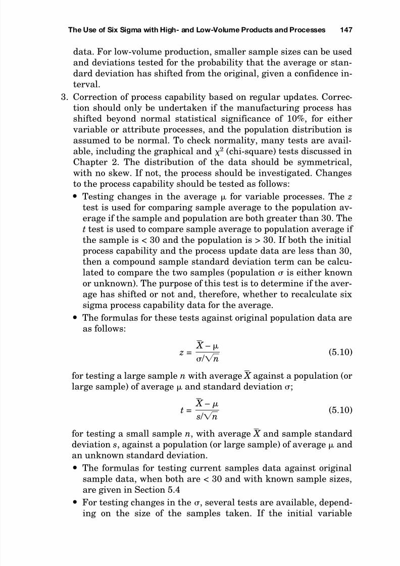
data. For low-volume production, smaller sample sizes can be used

and deviations tested for the probability that the average or stan-

dard deviation has shifted from the original, given a confidence in-

terval.

3. Correction of process capability based on regular updates. Correc-tion should only be undertaken if the manufacturing process has

shifted beyond normal statistical significance of 10%, for either

variable or attribute processes, and the population distribution is

assumed to be normal. To check normality, many tests are avail-

able, including the graphical and 2 (chi-square) tests discussed in

Chapter 2. The distribution of the data should be symmetrical,

with no skew. If not, the process should be investigated. Changes

to the process capability should be tested as follows:

Testing changes in the average for variable processes. The ztest is used for comparing sample average to the population av-

erage if the sample and population are both greater than 30. The

t test is used to compare sample average to population average if

the sample is < 30 and the population is > 30. If both the initial

process capability and the process update data are less than 30,

then a compound sample standard deviation term can be calcu-

lated to compare the two samples (population is either known

or unknown). The purpose of this test is to determine if the aver-

age has shifted or not and, therefore, whether to recalculate sixsigma process capability data for the average.

The formulas for these tests against original population data are

as follows:

z = (5.10)

for testing a large sample n with average X against a population (or

large sample) of average and standard deviation ;

t = (5.10)

for testing a small sample n, with average X and sample standard

deviation s, against a population (or large sample) of average and

an unknown standard deviation.

The formulas for testing current samples data against original

sample data, when both are < 30 and with known sample sizes,

are given in Section 5.4

For testing changes in the , several tests are available, depend-

ing on the size of the samples taken. If the initial variable

X –

s / n

X –

/ n

The Use of Six Sigma with High- and Low-Volume Products and Processes 147



process capability population data is greater than 30, and the ca-

pability update data is less than 30, then the 2 test can be used.

To compare current value of to the initial process capability

when both data sets are under 30, the F test should be used. F

tests can test for a level of significance (5% or 1%) to determine if the ’s between the two data sets are statistically different. De-

pending on the results of these tests, the six sigma attributes are

either retained or recalculated. The F test can also be used when

two or more sample data sets originate from a common popula-

tion. In that case, the differences between sample variability are

either due to natural variation or a deviation in the product.

More details on the F test are given in Chapter 7.

5.2.2 Determination of standard deviation forprocess capability

There are four different methods for determining the standard devia-

tion of the population for process capability studies:

1. Total overall variation. All data is collected into one large group

and treated as a single large sample with n greater than 30.

2. Within-group variation. Data is collected into subgroups, and a dis-

persion statistic is calculated (range). All ranges of each subgroup

are averaged into an R . The is calculated from an R estimator(d2). This method is the basis for variable control chart limit calcu-

lations and discussed in Chapter 3.

3. Between-group variation. Data is collected into subgroups, and an

average ( X ) is calculated for each subgroup. The standard devia-

tion s of sample averages is calculated. The population is esti-

mated from the central limit theorem equation, = s · n . This

method can be used to obtain process capability from control chart

limits.

4. Moving range method. In this method, data is collected into onegroup of small numbers of data, over time. A range ( R) is calculat-

ed from each two successive points. All ranges of each pair are av-

eraged into an R . The is calculated from an R estimator (d2) for n

= 2, which is equal 1.128. Method 4 is the preferred method for

time series data and small data sets from low-volume manufactur-

ing.

For processes that are in statistical control, these methods are equiv-

alent over time. For processes not in control, only Method is 2 insensi-tive to process variations of the average over time. The estimate is

inflated or deflated with Method 1 and could be severely inflated/de-




flated with Method 3. An example of a process out of control is one in

which one subgroup has a large sample average shift as opposed to

smaller average shifts in the other subgroups. Another way to advan-

tageously leverage Method 2 to negate the effect of average shift is to

use Method 4, with the data spread over time.

5.2.3 Example of methods of calculating

Example 5.10

Data for a production operation was collected in 30 samples, in three

subgroups, measured at different times. The four different methods of

calculating are as follows.

SubgroupSubgroup Measurement range(R) Average s

I 4, 3, 5, 5, 4, 8, 6, 4, 4, 7 5 5 1.56

II 2, 4, 5, 3, 7, 5, 4, 3, 2, 5 5 4 1.56

III 3, 6, 7, 6, 8, 4, 5, 4, 6, 6 5 5.5 1.51

Average of subgroups I–III 5 4.83 1.54

For the total group 6 4.83 1.62

Moving range for each subgroup Total R

I 1, 2, 0, 1, 4, 2, 2, 0, 3 15 1.67 1.48

II 2, 1, 2, 4, 2, 1, 1, 1, 3 17 1.89 1.68

III 3, 1, 1, 2, 4, 1, 1, 2, 0 15 1.67 1.48

Average moving range 1.74 1.54

Method 1. Total overall variation of 30 data points from 3 sub-

groups

2 = = = [777 – (145)2 /30]/29 = 2.626

= 1.62

Method 2. Within-group variation; R = 5 (n = 10)

= R / d2(n=10) = 5/3.078 = 1.62

Method 3. Between-group variation

s( X ) = (5, 4, 5.5) = 0.763

= s · n = 0.764 · 1 0 = 2.415

i y i

2 – (i yi)2 / n

n – 1

i( yi – y )2

n – 1

The Use of Six Sigma with High- and Low-Volume Products and Processes 149



Method 4. Moving range method (n = 2)

For each subgroup, obtain the average range between successive

numbers:

Subgroup I: = R

/ d2(n=2) = 1.67/1.128 = 1.48Subgroup II: = R / d = 1.89/1.128 = 1.68

Subgroup III: = R / d = 1.67/1.128 = 1.48

2

2

For the total groups (I–III), = R / d = 1.74/1.128 = 1.54.

As can be seen from Example 5.10, the of the overall 30 numbers

was 1.62 (Method 1). The 30 numbers were made of three subgroups

(samples) with large shifts in sample averages. The closest indirectly

calculated value was obtained by Method 2, between-group varia-

tion from the R estimator of , because it negated the average shifts.The moving range method (Method 4) was as much as 10% off, even

when using the full 30 numbers. The least accurate value was Method

3, the between-group variation, which derived from a distribution of

sample averages and the conversion of the sample to population .

The number of subgroups (samples) was small and led to the largest

error in determination.

––2

5.2.4 Process capability for low-volume production

When it is not feasible to collect the amount of data required to deter-

mine process capability because of cost or resource issues or produc-

tion volume, reduced data can be used successfully to estimate

process capability, provided that confidence is quantified in the data

analysis. Although 30 points of data are considered statistically sig-

nificant, a smaller number of data points can be taken, using prede-

termined error levels and confidence goals, to obtain a good estima-

tion of process average and variability. Refer to earlier sections in this

chapter for proper methods and examples.

The moving range method provides an alternate mechanism for es-timating the for small amounts of data, provided that data points

are taken over time for both variable and attribute processes. Ten

data point are required to provide an estimator for with the moving

range method.


Documents

Process Capability for Large-Volume Production