Embed Size (px)
Citation preview

Economic Model Predictive Control with Extended Horizon
by
Su Liu
A thesis submitted in partial fulfillment of the requirements for the degree of
Doctor of Philosophy
in
Process Control
Department of Chemical and Materials Engineering
University of Alberta
c©Su Liu, 2017

Abstract
In this thesis, we propose a computationally efficient economic model predictive con-
trol (EMPC) design which is based on a well-known methodology — the separation of
the control and prediction horizon. The extension of the prediction horizon of EMPC
is realized by employing an auxiliary control law which asymptotically stabilizes the
optimal steady state. The contributions of this thesis are to systematically analyze
the stability and performance of the general EMPC scheme with extended horizon,
and to explore its extensions and applications to several specific scenarios.
Specifically, we establish stabilizing conditions of the proposed EMPC in a pro-
gressive manner. First, we establish practical stability of the EMPC with respect
to the extended horizon for strictly dissipative systems satisfying mild assumptions.
Then, under stronger conditions involving Lipschitz continuities and exponential sta-
bility of the auxiliary controller, the shrinkage of the practical stability region is
shown to be exponential. Further, we characterize a general condition on the stor-
age function under which exponential stability of the optimal steady state can be
established. Conventional set-point tracking MPC with quadratic cost falls into the
latter category. The achievable performance of the proposed EMPC design is also
discussed in a similar manner under different stabilizing conditions. It is revealed
that the performance of the proposed EMPC is approximately upper-bounded by the
auxiliary controller. Our theoretical results provide valuable insights into the intrinsic
properties of EMPC as the discussions are laid out in a very general setting and the
results are compatible with the analysis of existing MPC / EMPC designs.
With a deepened theoretical understanding of EMPC with extended horizon, we
further explored the extension of the proposed EMPC design in several scenarios: (i)
We consider the case where a locally optimal LQR control law can be found. A termi-
nal cost is constructed as the value function of the LQR controller plus a linear term
ii

characterized by the Lagrange multiplier associated with the steady-state constraint.
This design results in an EMPC this is locally optimal. (ii) We take advantage of
EMPC with extended horizon to handle systems with scheduled switching operations.
The EMPC operations are divided into two phases — an infinite-time operation phase
and a mode transition phase. The proposed EMPC schemes are much more efficient
and achieves improved mode transition performance than existing EMPC designs.
(iii) We consider systems with zone tracking objectives which can be viewed as a
special case of economic objective. The proposed zone MPC penalizes the distance
of the predicted state and input trajectories to a desired target zone which is not
necessarily positive invariant. We resort to LaSalle’s invariance principle and develop
invariance-like theorem which is suitable for stability analysis of zone control. Auxil-
iary controllers which asymptotically stabilize an invariant subset of the target zone
are employed to enlarge the region of attraction. (iv) We apply the proposed EMPC
algorithm to the control of oilsand primary separation vessel (PSV) to maximize the
bitumen recovery rate.
iii

Preface
The materials presented in this thesis are part of the research project under the
supervision of Dr. Jinfeng Liu, and is funded by Alberta Innovates Technology Futures
(AITF) and Natural Sciences and Engineering Research Council (NSERC) of Canada.
Chapter 2 of this thesis is a revised version of Su Liu and Jinfeng Liu, Economic
model predictive control with extended horizon. Automatica, 73:180-192, 2016.
Chapter 3 of this thesis is a revised version of Su Liu and Jinfeng Liu. A terminal
cost for economic model predictive control with local optimality. In Proceedings of
the American Control Conference, pages 1954-1959, Seattle, WA, 2017.
Chapter 4 of this thesis is a revised version of Su Liu and Jinfeng Liu. Economic
model predictive control for scheduled switching operations. In Proceedings of the
American Control Conference, pages 1784-1789, Boston, MA, 2016.
Chapter 5 of this thesis is a revised version of Su Liu, Yawen Mao, and Jinfeng
Liu, Nonlinear model predictive control for zone tracking. IEEE Transactions on
Automatic Control, submitted.
Chapter 6 of this thesis is a revised version of Su Liu, Jing Zhang and Jinfeng Liu.
Economic MPC with terminal cost and application to an oilsand primary separation
vessel. Chemical Engineering Science, 136:27-37, 2015.
iv
Acknowledgements
Foremost, I would like to express my sincere gratitude to my supervisor Professor
Jinfeng Liu for providing me with an excellent atmosphere for doing research. He
has been a role model to me as a researcher, mentor and instructor. This thesis
would not have been possible without his competent guidance, constant availability
and wholehearted support.
Besides my supervisor, I would like to thank my committee members Profes-
sor Vinay Prasad, Professor Biao Huang, Professor Qing Zhao and Professor Luis
Ricardez-Sandoval for their interest in my work.
I would also like to thank members from our research group who have helped me
along the way: Jing Zhang, Xunyuan Yin, Tianrui An, Kevin Arulmaran, Jayson
McAllister, An Zhang, Nirwair Bajwa, Yawen Mao, Jannatun Nahar and Benjamin
Decardi-Nelson. I also wish to thank my friends who have made life at the University
of Alberta a wonderful experience: Lin Shao, Lei Yao, Ruomu Tan, Wenhan Shen,
Shunyi Zhao, Tianbo Liu, Xin Xu.
I gratefully acknowledge the financial support from Natural Sciences and Engi-
neering Research Council of Canada (NSERC) and Alberta Innovative Technology
Futures (AITF).
I would like to thank my girlfriend, Huan Huang, for her companion on our journey
of self-discovery. Last but not least, my deepest gratitude goes to my mother, Yuehe
Zhou, whose unconditional love and inner beauty has been my greatest source of
strength.
v

Contents
1 Introduction 1
1.1 Motivation . . . . . . . . . . . . . . . . . . . . . . . . . . . . . . . . . 1
1.2 Research overview . . . . . . . . . . . . . . . . . . . . . . . . . . . . . 2
1.2.1 A brief review of MPC . . . . . . . . . . . . . . . . . . . . . . 2
1.2.2 Separation of control and prediction horizon . . . . . . . . . . 4
1.2.3 Economic MPC . . . . . . . . . . . . . . . . . . . . . . . . . . 5
1.3 Contributions and thesis outline . . . . . . . . . . . . . . . . . . . . . 6
2 Economic MPC with extended horizon 9
2.1 Problem setup . . . . . . . . . . . . . . . . . . . . . . . . . . . . . . . 10
2.1.1 Notation . . . . . . . . . . . . . . . . . . . . . . . . . . . . . . 10
2.1.2 System description . . . . . . . . . . . . . . . . . . . . . . . . 10
2.1.3 EMPC based on an auxiliary controller . . . . . . . . . . . . . 10
2.2 Stability and convergence . . . . . . . . . . . . . . . . . . . . . . . . 13
2.2.1 Practical stability . . . . . . . . . . . . . . . . . . . . . . . . . 13
2.2.2 Exponential shrinkage . . . . . . . . . . . . . . . . . . . . . . 21
2.3 Asymptotic and transient performance . . . . . . . . . . . . . . . . . 27
2.3.1 Asymptotic performance . . . . . . . . . . . . . . . . . . . . . 28
2.3.2 Transient performance . . . . . . . . . . . . . . . . . . . . . . 30
2.4 Numerical examples . . . . . . . . . . . . . . . . . . . . . . . . . . . . 38
2.5 Summary . . . . . . . . . . . . . . . . . . . . . . . . . . . . . . . . . 42
3 Economic MPC with local optimality 45
3.1 Preliminaries . . . . . . . . . . . . . . . . . . . . . . . . . . . . . . . 45
3.1.1 Notation . . . . . . . . . . . . . . . . . . . . . . . . . . . . . . 45
vi

3.1.2 System description . . . . . . . . . . . . . . . . . . . . . . . . 46
3.2 Optimal operation of the system . . . . . . . . . . . . . . . . . . . . . 46
3.3 EMPC with the proposed terminal cost . . . . . . . . . . . . . . . . . 51
3.4 Case study . . . . . . . . . . . . . . . . . . . . . . . . . . . . . . . . . 55
3.5 Summary . . . . . . . . . . . . . . . . . . . . . . . . . . . . . . . . . 57
4 Economic MPC for scheduled switching operations 60
4.1 Preliminaries . . . . . . . . . . . . . . . . . . . . . . . . . . . . . . . 61
4.1.1 Notation . . . . . . . . . . . . . . . . . . . . . . . . . . . . . . 61
4.1.2 System description . . . . . . . . . . . . . . . . . . . . . . . . 61
4.1.3 A set of auxiliary controllers . . . . . . . . . . . . . . . . . . . 62
4.2 Proposed empc for scheduled switching operations . . . . . . . . . . . 63
4.2.1 Implementation strategy . . . . . . . . . . . . . . . . . . . . . 64
4.2.2 Proposed EMPC design . . . . . . . . . . . . . . . . . . . . . 66
4.2.3 Recursive feasibility . . . . . . . . . . . . . . . . . . . . . . . . 68
4.3 Application to a chemical process . . . . . . . . . . . . . . . . . . . . 70
5 Nonlinear MPC for zone tracking 74
5.1 Introduction . . . . . . . . . . . . . . . . . . . . . . . . . . . . . . . . 74
5.2 Problem setup . . . . . . . . . . . . . . . . . . . . . . . . . . . . . . . 76
5.2.1 Notation . . . . . . . . . . . . . . . . . . . . . . . . . . . . . . 76
5.2.2 System description and control objective . . . . . . . . . . . . 76
5.3 Zone MPC formulation . . . . . . . . . . . . . . . . . . . . . . . . . . 77
5.4 Stability analysis . . . . . . . . . . . . . . . . . . . . . . . . . . . . . 78
5.5 Further discussions . . . . . . . . . . . . . . . . . . . . . . . . . . . . 83
5.5.1 Enlargement of the region of attraction . . . . . . . . . . . . . 83
5.5.2 Handling a secondary economic objective . . . . . . . . . . . . 86
5.6 Examples . . . . . . . . . . . . . . . . . . . . . . . . . . . . . . . . . 87
5.7 Summary . . . . . . . . . . . . . . . . . . . . . . . . . . . . . . . . . 91
6 Application to an Oilsand Primary Separation Vessel 93
6.1 Preliminaries . . . . . . . . . . . . . . . . . . . . . . . . . . . . . . . 93
6.1.1 Notation . . . . . . . . . . . . . . . . . . . . . . . . . . . . . . 93
vii

6.1.2 System description . . . . . . . . . . . . . . . . . . . . . . . . 94
6.1.3 Stability assumption . . . . . . . . . . . . . . . . . . . . . . . 94
6.2 EMPC with terminal cost . . . . . . . . . . . . . . . . . . . . . . . . 95
6.2.1 Properties of the nonlinear controller h(x) . . . . . . . . . . . 95
6.2.2 Proposed EMPC design . . . . . . . . . . . . . . . . . . . . . 97
6.2.3 Stability and performance analysis . . . . . . . . . . . . . . . 99
6.3 Fixed-time implementation . . . . . . . . . . . . . . . . . . . . . . . . 103
6.3.1 Implementation strategy . . . . . . . . . . . . . . . . . . . . . 103
6.3.2 Stability and performance analysis . . . . . . . . . . . . . . . 104
6.4 Application to a primary separation vessel . . . . . . . . . . . . . . . 107
6.4.1 Process description and modeling . . . . . . . . . . . . . . . . 107
6.4.2 EMPC design . . . . . . . . . . . . . . . . . . . . . . . . . . . 109
6.4.3 Simulation result . . . . . . . . . . . . . . . . . . . . . . . . . 113
6.5 Summary . . . . . . . . . . . . . . . . . . . . . . . . . . . . . . . . . 119
7 Conclusions and Future Work 120
7.1 Conclusions . . . . . . . . . . . . . . . . . . . . . . . . . . . . . . . . 120
7.2 Future research directions . . . . . . . . . . . . . . . . . . . . . . . . 122
viii

List of Tables
2.1 Shifted asymptotic performance (Jasy−l(xs, us)) and average optimiza-
tion evaluation time (CPU) of the proposed EMPC with N = 1 . . . 40
2.2 Shifted asymptotic performance (Jasy−l(xs, us)) and average optimiza-
tion evaluation time (CPU) of the EMPC without terminal cost. . . . 41
2.3 Transient performance (J30) and optimization evaluation time (CPU)
of the proposed EMPC with terminal cost with N = 1. . . . . . . . . 42
2.4 Transient performance (J30) and optimization evaluation time (CPU)
of the EMPC without terminal cost. . . . . . . . . . . . . . . . . . . 43
3.1 Process parameters . . . . . . . . . . . . . . . . . . . . . . . . . . . . 55
3.2 Process parameters . . . . . . . . . . . . . . . . . . . . . . . . . . . . 57
4.1 Model parameters. . . . . . . . . . . . . . . . . . . . . . . . . . . . . 71
4.2 Performance under different configurations . . . . . . . . . . . . . . . 73
4.3 Average controller evaluation time . . . . . . . . . . . . . . . . . . . . 73
5.1 The transient performance of the four zone MPC configurations over
30 sampling times . . . . . . . . . . . . . . . . . . . . . . . . . . . . . 88
6.1 Process variables. . . . . . . . . . . . . . . . . . . . . . . . . . . . . . 110
6.2 Model parameters. . . . . . . . . . . . . . . . . . . . . . . . . . . . . 111
6.3 Steady-state operating point. . . . . . . . . . . . . . . . . . . . . . . 111
6.4 Transient and steady-state average bitumen recovery rates of the closed-
loop system under the proposed EMPC with terminal cost, the EMPC
in [1], the tracking MPC and the controller h(x) . . . . . . . . . . . 113
ix

6.5 Average bitumen recovery rates of the closed-loop system under (a):
the infinite-time implementation, (b): fixed-time implementation, (c):
alternative fixed-time implementation, and (d): the controller h(x). . 116
x

List of Figures
1.1 A conceptual picture of the MPC scheme . . . . . . . . . . . . . . . . 3
2.1 Closed-loop system state trajectories under the proposed EMPC with
N = 1 and Nh = 1, 5, 10, 15, 20 (solid lines), EMPC without terminal
cost with N = 1, 5, 10, 15, 20 (dashed lines), and the auxiliary
controller h (dash-dotted line). . . . . . . . . . . . . . . . . . . . . . . 39
2.2 Transient performance under the proposed EMPC with N = 1 and
Nh = 1, 5, 10 (solid lines), EMPC without terminal cost with N =
1, 5, 10 (dashed lines), and the auxiliary controller h (dash-dotted line). 40
2.3 State trajectories of the closed-loop system under the proposed EMPC
with N = 1 and Nh = 1, 2, 5 (solid lines), EMPC without terminal
cost with N = 1, 5, 10, 15, 20 (dashed lines), and the auxiliary
controller h (dash-dotted line). . . . . . . . . . . . . . . . . . . . . . . 42
2.4 Stage costs of the closed-loop system under the proposed EMPC with
N = 1 and Nh = 1, 2, 5 (solid lines), EMPC without terminal cost
with N = 1, 5, 10, 15, 20 (dashed lines), and the auxiliary controller
h (dash-dotted line). . . . . . . . . . . . . . . . . . . . . . . . . . . . 43
3.1 Closed-loop state trajectories under EMPC with the proposed terminal
cost (solid lines), EMPC without terminal cost (dashed lines), and
EMPC with terminal cost for stability [2] (dash-dotted line). . . . . . 57
3.2 Closed-loop input trajectories under EMPC with the proposed terminal
cost (solid lines), EMPC without terminal cost (dashed lines), and
EMPC with terminal cost for stability [2] (dash-dotted line). . . . . . 58
xi

3.3 Closed-loop stage costs under EMPC with the proposed terminal cost
(solid lines), EMPC without terminal cost (dashed lines), and EMPC
with terminal cost for stability [2] (dash-dotted line). . . . . . . . . . 58
4.1 Time flow of Algorithm 1 . . . . . . . . . . . . . . . . . . . . . . . . . 65
4.2 Closed-loop state trajectories of the proposed approach (solid lines),
the approach in [3] (dashed lines) and the auxiliary controllers (dash-
dotted line). . . . . . . . . . . . . . . . . . . . . . . . . . . . . . . . 72
4.3 Closed-loop input trajectories of the proposed approach (solid line), the
approach in [3] (dashed line) and the auxiliary controllers (dash-dotted
line). . . . . . . . . . . . . . . . . . . . . . . . . . . . . . . . . . . . 73
5.1 Closed-loop state trajectory under controller u = h(x): for any initial
state x ∈ Xh, the trajectory xh(k, x) enters the positive invariant set
XMt,h in Nh steps and is maintained in it thereafter. . . . . . . . . . . . 85
5.2 State and input trajectories of a): a zone MPC that tracks the target
zone Zt (diamonds), b): a zone MPC that tracks the largest control in-
variant set in the target zone ZMt (squares), c): the proposed zone MPC
of Eq. (5.2) (triangles), and d): the proposed zone MPC of Eq. (5.7)
(circles). . . . . . . . . . . . . . . . . . . . . . . . . . . . . . . . . . . 88
5.3 State and input trajectories of set-point MPC. . . . . . . . . . . . . . 90
5.4 State and input trajectories of the zone MPC. . . . . . . . . . . . . . 90
5.5 State and input trajectories of set-point MPC. . . . . . . . . . . . . . 90
5.6 State and input trajectories of the zone MPC. . . . . . . . . . . . . . 91
5.7 Bifurcation diagram of system (5.10). The bifurcation diagram shows
the the values of system state x(n) that are visited or approached
asymptotically under a constant u(n). For u ∈ (−0.75,−0.6], the
system has stable steady-state operation. At u = −0.75, steady-state
operation becomes unstable and the diagram bifurcates into two points
which corresponds to a stable periodic operation of period two. As the
value of u decreases, more bifurcation occurs and at some point around
u = −1.4 the system enters a chaotic operating region. The dashed
line corresponds to steady-state operating points . . . . . . . . . . . . 92
xii

6.1 Schematic of the primary separation vessel . . . . . . . . . . . . . . . 107
6.2 Bitumen recovery rate trajectores of the closed-loop system under the
proposed EMPC with terminal cost (dashed line), the EMPC in [1]
(dotted line), the tracking MPC (dash dotted line) and the controller
h(x) (solid line). . . . . . . . . . . . . . . . . . . . . . . . . . . . . . . 114
6.3 Froth layer volume trajectores of the closed-loop system under the
proposed EMPC with terminal cost (dashed line), the EMPC in [1]
(dotted line), the tracking MPC (dash dotted line) and the controller
h(x) (solid line). . . . . . . . . . . . . . . . . . . . . . . . . . . . . . . 114
6.4 Lyapunov function trajectores of the closed-loop system under the pro-
posed EMPC with terminal cost (dashed line), the EMPC in [1] (dot-
ted line), the tracking MPC (dash dotted line) and the controller h(x)
(solid line). . . . . . . . . . . . . . . . . . . . . . . . . . . . . . . . . 115
6.5 Input trajectories of the closed-loop system under the proposed EMPC
with terminal cost (dashed line), the EMPC in [1] (dotted line), the
tracking MPC (dash dotted line) and the controller h(x) (solid line). . 115
6.6 Bitumen recovery rates of the closed-loop system under the infinite-
time implementation (dashed line), fixed-time implementation(dotted
line), alternative fixed-time implementation (dash dotted line) and the
controller h(x) (solid line). . . . . . . . . . . . . . . . . . . . . . . . . 117
6.7 Froth layer volume trajectories of the closed-loop system under the
infinite-time implementation (dashed line), fixed-time implementation(dotted
line), alternative fixed-time implementation (dash dotted line) and the
controller h(x) (solid line). . . . . . . . . . . . . . . . . . . . . . . . . 117
6.8 Lyapunov function trajectories of the closed-loop system under the
infinite-time implementation (dashed line), fixed-time implementation(dotted
line), alternative fixed-time implementation (dash dotted line) and the
controller h(x) (solid line). . . . . . . . . . . . . . . . . . . . . . . . . 118
6.9 Input trajectories of the closed-loop system under the infinite-time
implementation (dashed line), fixed-time implementation(dotted line),
alternative fixed-time implementation (dash dotted line) and the con-
troller h(x) (solid line). . . . . . . . . . . . . . . . . . . . . . . . . . . 118
xiii

Chapter 1
Introduction
1.1 Motivation
Model predictive control (MPC) is a rich fruit in the branch of model control theory
which is rooted in computer science and informatics. Ever since its origin in chemical
plants in the late 1970s, both the industrial applications and theory development of
MPC have been booming. A survey [4] conducted in mid-1999 showed more than
4500 industrial MPC applications prior to the new millennium and indicated a rapid
annual growth of approximately 20%. Presently, not only has MPC become the stan-
dard advanced control technique in chemical engineering, it is also being applied to
various areas in mechanical engineering, electrical engineering, automotive engineer-
ing, aerospace engineering and so on. The landscape of MPC is shaped by three major
aspects: theory, computation and application. To a large extent, early development
of MPC theory was pushed by its successful industrial applications. The progresses in
MPC theory in return stimulated more applications which forms a positive feedback
loop. Since the implementation of MPC requires online or real-time optimization,
all MPC designs and applications have to reckon with the computational burden.
This entails either the use of more powerful optimization algorithms or the design of
computationally efficient MPC.
Traditionally, in the process industry, MPC is designed for tracking set-point or
reducing variations in crucial process variables. The huge success of MPC in indus-
trial applications owes much to its ability to optimally handle process constraints and
interactions. However, in many applications, especially at a higher level of decision-
making, the objectives are often economic-oriented and may be different from the
1

classical control objective of set-point tracking. For example, some typical objec-
tives include the maximization of operation profit, the minimization of energy con-
sumption, or the maximization of a certain product. These economic objectives may
not be seamlessly translated into set-point tracking objectives. It is possible that
non steady-state operation, such as periodic operation, yields superior performance.
These considerations motivate the recent development of a more general form of MPC
called economic MPC or EMPC. EMPC optimizes general cost functions that are di-
rectly linked to the economic metrics (profit, efficiency, sustainability) of the plant.
This promising approach, which has great potential to improve the dynamic perfor-
mance during transient processes, is still a relatively new research area. New theories,
algorithms and tools are being developed for EMPC.
In this thesis, we propose a computationally efficient EMPC design which is based
on a well-known methodology in conventional MPC — separation of the control and
prediction horizon. Our objectives are to systematically analyze the stability and
performance of the general EMPC scheme with extended horizon, and to explore its
extensions and applications to several specific scenarios.
1.2 Research overview
1.2.1 A brief review of MPC
Technically, MPC refers to a control methodology that repeatedly solves online a
finite-horizon open-loop optimal control problem in a receding horizon fashion. Fig-
ure 1.1 shows a conceptual picture of the MPC scheme. At a sampling time k, the
MPC algorithm computes a future input trajectory by optimizing the predicted tra-
jectories over a finite prediction horizon with the initial state x(k). The first element
of the input sequence is then injected to the plant. Upon availability of an updated
state measurement (or estimation) at the subsequent sampling time k + 1, the MPC
algorithm is repeated with the prediction horizon shifted one step further.
MPC differs from the classical optimal control mainly in the way the optimal con-
trol problem is solved. In classical optimal control such as LQR control, an optimal
feedback control law is obtained offline whereas in MPC, an input sequence is calcu-
lated online based on the current system state. The former requires the solution of the
2

FuturePast
Reference trajectory/Set-point
Predicted trajectories
Predicted horizon
… ...
Computed future input trajectory
k
( )x k
1k k N
Figure 1.1: A conceptual picture of the MPC scheme
Hamilton-Jacobi-Bellman equation which can be very difficult or merely impossible
to obtain for generic nonlinear systems. The latter amounts to solving a finite di-
mensional mathematical programming problem in real-time which is becoming more
and more viable thanks to the development of computer hardware/software and the
advances in optimization algorithms.
An essential feature that shapes the landscape of MPC theory and design is that
the open-loop optimal control problem be solvable in a short period of time (as com-
pared to the dynamics of the process). For one thing, online optimization necessitates
the use of a finite horizon which creates a discrepancy between MPC theory and clas-
sical infinite-horizon optimal control. This discrepancy has spawned considerable
research interests in the design and analysis of MPC with nominal stability guaran-
tee. Consensus was reached in the milestone paper [5] in which the use of the value
function as Lyapunov function and several ‘ingredients’ for nominal stability of MPC
are formalized. Since then, more insights into the inherent stability of MPC have
been revealed by leveraging the dynamic programming principle [6], [7], [8], [9], [10].
For another thing, computational efficiency of MPC will remain a constant theme
throughout the development of MPC. This is a twofold mission. On the one hand, de-
velopment of fast optimization algorithms serve as the most straightforward impetus
for the computational efficiency of MPC. The majority of industrial MPC optimiza-
3

tion problems are formulated as quadratic programming (QP) problems which can
be efficiently solved using standard algorithms such as the interior-point methods
[11, 12], the active-set method [13], and fast gradient methods [14]. Recent advances
in nonlinear programming has also made online implementation of MPC to nonlin-
ear, large-scale systems possible, promoting an integrated MPC scheme for plant-wide
real-time optimization [15]. On the other hand, significant research efforts have been
made to reduce the computational load of MPC. These include heated research areas
such as (i) distributed MPC (see [16] and the references therein), where a centralized
MPC is decomposed into several subsystem MPCs which communicate and cooper-
ate; and (ii) explicit MPC (e.g., [17], [18]), where an explicit feedback control law
is obtained offline by solving a parametric programming problem or obtaining its
approximate solution.
1.2.2 Separation of control and prediction horizon
One of the most commonly adopted approach to improve the computational efficiency
of MPC is to separate the control horizon and the prediction horizon. The idea is to
extend the prediction horizon beyond the control horizon by employing an auxiliary
control law which asymptotically stabilizes the desired set-point. In this way, the
optimization horizon of MPC can be increased without increasing the number of
decision variables (i.e. the number of free inputs). As a matter of fact, separation
between the control horizon and the prediction horizon arises along early versions of
MPC and is well embraced in industrial MPC [4]. With the development of MPC
theory, however, separation between the control horizon and the prediction horizon
is gradually being phased out in the context of linear MPC. It was shown in [19] that
the constrained infinite-horizon LQR can be formulated as a finite-dimensional QP.
Specifically, the infinite-horizon tail of the LQR objective function can be lumped
together as a terminal cost function which is the value function of an unconstrained
infinite-horizon LQR. Under this design, if the control horizon is sufficiently large
such that the predicted state at the end of the control horizon can be steered to the
origin by the unconstrained infinite-horizon LQR without violating state and input
constraints, then the MPC is equivalent to the optimal constrained infinite-horizon
LQR controller. The availability of the locally optimal terminal cost function as well
4

as the efficient QP algorithms mentioned above make the separation between control
and prediction horizon less appealing for linear MPC designs.
However, for nonlinear systems, the infinite-horizon cost-to-go is in general not
available because the solution to the corresponding HJB equation may not exist. A
practical remedy is to use a control Lyapunov function (CLF) which provides an
incremental upper bound on the stage cost [20, 21, 7] as the terminal cost function.
NMPC designed this way has guaranteed stability but can be overly conservative,
especially when the terminal cost is much larger than the actual infinite-horizon cost-
to-go. Theoretically, one could use a large control horizon to achieve asymptotic
stability as well as near-optimal performance [6, 8, 22]. But the use of a large control
horizon poses serious challenge to the computational efficiency of MPC. An ideal
trade-off is proposed in [23], where a locally optimal control law is utilized to extend
the prediction horizon of the NMPC design. The NMPC in [23] is capable of achieving
enlarged stability region and locally optimal performance without relying on a large
control horizon. These desired features of NMPC design are only possible via the
separation of control and prediction horizons. It is therefore safe to say that the
methodology to separate control and prediction horizon bears its indispensable merits
in the context of NMPC design.
1.2.3 Economic MPC
With the maturing of MPC theory, recent development of MPC has seen an explo-
ration into economic-oriented model predictive control. This line of research originates
from [24] where unreachable set-points are considered in the conventional tracking
MPC scheme. The authors showed that tracking unreachable set-point results in
improved transient performance as compared to the conventional MPC that tracks
reachable set-point. These results simulated research efforts into a novel form of
MPC called economic MPC (EMPC). In EMPC, the quadratic-type cost functions
used in conventional MPC are replaced with general economic cost functions that
are not necessarily positive-definite with respect to the optimal steady-state opera-
tion. Consequently, standard stability analysis techniques to use the value function
of conventional MPC as a Lyapunov function is no longer viable. In fact, steady-state
operation may not even be the economically optimal operation for EMPC. It has been
5

realized that dissipativity plays an important role in characterizing the optimality of
steady-state operation as well as establishing the stability of EMPC [25, 26, 27].
Different EMPC designs have been proposed which stem from the conventional
NMPC designs. For example, EMPC with point-wise terminal constraint [28], EMPC
with terminal cost [2, 29], EMPC with Lyapunov-based constraint [30, 1]. These
EMPC designs also suffer the problems encountered in the conventional NMPC design
— they could be overly conservative or computationally demanding. In another
line of research [10, 31], EMPC without terminal conditions is studied. This line of
research reveals some intrinsic properties of EMPC. It is shown that under certain
controllability and dissipativity conditions, near-optimal performance can be achieved
if a sufficiently large control horizon is used. However, a large control horizon could
make online implementations of the EMPC design computationally impractical. It is
thus natural to also resort to the separation of control and prediction horizon in the
context of EMPC to improve its computational efficiency.
1.3 Contributions and thesis outline
The rest of the thesis is organized as follows:
In Chapter 2, we propose the basic EMPC formulation with extended prediction
horizon based on an auxiliary controller. The extension of the prediction horizon is
realized by employing a terminal cost which characterizes the economic performance
of the auxiliary controller over a finite prediction horizon. The proposed EMPC
design is easy to construct and computationally efficient. We analyze the stability
and performance of the proposed EMPC design with special attention paid to the
impact of the extended horizon. It is shown that for strictly dissipative systems
satisfying mild assumptions, a finite terminal horizon is sufficient to guarantee the
convergence and performance of the EMPC to be approximately upper-bounded by
that of the auxiliary controller.
In Chapter 3, we design a terminal cost for economic model predictive control
(EMPC) which preserves local optimality. From the results in Chapter 2, the perfor-
mance of EMPC is upper-bounded by the auxiliary controller. A very natural ques-
tion to ask is whether it is possible to find a locally optimal control law and whether
6

the corresponding infinite-horizon cost to go or its approximation can be found. We
first show, based on the strong duality and second order sufficient condition (SOSC)
of the steady-state optimization problem, that the optimal operation of the system
is locally equivalent to an infinite-horizon LQR controller. The proposed terminal
cost is constructed as the value function of the LQR controller plus a linear term
characterized by the Lagrange multiplier associated with the steady state constraint.
EMPC with the proposed terminal cost is stabilizing with an appropriately chosen
control horizon, and preserves the local optimality of the LQR controller. Simulation
results of an isothermal CSTR verify our analysis.
In Chapter 4, we extend the proposed EMPC design to control systems with sched-
uled switching operations. The proposed EMPC scheme takes advantage of a set of
auxiliary controllers that locally stabilizes the optimal steady state of each operating
mode. In the proposed approach, EMPC operations are divided into two phases — an
infinite-time operation phase and a mode transition phase, depending on the current
sampling time and the scheduled mode switching time. Sufficient conditions to en-
sure recursive feasibility of the proposed EMPC design are established. The proposed
EMPC design is computationally efficient and enjoys enlarged feasibility regions than
the auxiliary controllers. Simulation results of a chemical process example demon-
strate the superiority of our design over existing MPC designs for switched scheduling
operations.
In Chapter 5, we propose a general framework for the design and analysis of
nonlinear model predictive control for zone tracking. Zone tracking objective can be
viewed as a special case of economic objective. The proposed zone MPC penalizes
the distance of the predicted state and input trajectories to a desired target zone
which is not necessarily positive invariant. We resort to the invariance principle
and develop invariance-like theorem which is suitable for stability analysis of zone
control. It is proved that under the zone MPC design, the system converges to the
largest control invariant subset of the target zone. Further discussions are made on
enlargement of the region of attraction by employing an auxiliary controller as well
as handling a secondary economic objective via a second-step economic optimization.
Two numerical examples are used to demonstrate the superiority of zone control over
set-point control and the efficacy of the zone MPC design.
7

In Chapter 6, we apply the proposed EMPC algorithm to an oilsand primary sep-
aration vessel (PSV). We show how previously developed EMPC design and analysis
results in the context of discrete-time system can be extended to continuous-time
systems where the issue of sampling needs to be addressed.
Chapter 7 summaries the contributions of this work and discusses future research
directions.
8

Chapter 2
Economic MPC with extendedhorizon
In this chapter, we propose the basic EMPC formulation with extended prediction
horizon based on an auxiliary controller. The system and EMPC formulation are
set up in Section 2.1. Section 2.2 addresses the stability and convergence of the
EMPC design. Practical stability of the proposed EMPC design is established for
strictly dissipative systems satisfying mild assumptions. Under stronger conditions,
the shrinkage of the practical stability region is shown to be exponential with respect
to the increase of the terminal horizon. For a special type of systems which satisfy a
further condition on the storage function (including conventional MPC with quadratic
cost), exponential stability can be achieved. Interestingly, the same result for this type
of systems may not be achieved by an EMPC without terminal condition. Section 2.3
discusses the asymptotic and transient performance of the EMPC design. Results
on the asymptotic performance of the proposed EMPC design for general nonlinear
systems are provided first. Stronger results on the transient performance of the EMPC
design for strictly dissipative systems are derived subsequently, based on different
stability conditions from Section 2.2. Two numerical examples are used to verify our
results in Section 2.4. Finally, we conclude our results in Section 2.5.
9

2.1 Problem setup
2.1.1 Notation
Throughout this work, the operator | · | denotes the Euclidean norm of a scalar or a
vector. The symbol ‘\’ denotes set substraction such that A \ B := x ∈ A, x /∈ B.
The symbol Br(xs) denotes the open ball centered at xs with radius r such that
Br(xs) := x : |x − xs| < r. A continuous function α : [0, a) → [0,∞) is said
to belong to class K if it is strictly increasing and satisfies α(0) = 0. A class K
function α is called a class K∞ function if α is unbounded. A continuous function
σ : [0,∞)→ [0, a) is said to belong to class L if it is strictly decreasing and satisfies
limx→∞
σ(x) = 0. A continuous function β : [0, a) × [0,∞) → [0,∞) is said to belong
to class KL if for each fixed r, β(r, s) belongs to class L, and for each fixed s, β(r, s)
belongs to class K.
2.1.2 System description
We consider a class of nonlinear systems which can be described by the following
discrete state-space model:
x(k + 1) = f(x(k), u(k)) (2.1)
where x ∈ Rnx denotes the state vector and u ∈ Rnu denotes the control input
vector. The system state and input are subject to the constraints x ∈ X and u ∈ U
respectively, where X ⊂ Rnx and U ⊂ Rnu are compact sets. We assume that there
exists an optimal steady state (xs, us) that uniquely solves the following steady-state
optimization problem:(xs, us) = arg min
x,ul(x, u)
s.t. x = f(x, u)x ∈ Xu ∈ U
(2.2)
where l(x, u) : X× U→ R is the economic stage cost function.
2.1.3 EMPC based on an auxiliary controller
It is assumed that there exists an auxiliary explicit controller u = h(x) which renders
xs asymptotically stable with us = h(xs) while satisfying the input constraint for
10

all x ∈ Xf , where Xf ⊆ X is a compact set containing xs in its interior. It is
also assumed that the region Xf is forward invariant under the controller u = h(x).
Namely, f(x, h(x)) ∈ Xf holds for all x ∈ Xf . We use xh(k, x) to denote the closed-
loop state trajectory under the controller h at time instant k with the initial state
xh(0, x) = x. The above assumptions imply that there exists a class KL function βx
such that:|xh(k, x)− xs| ≤ βx(|x− xs|, k)
xh(k, x) ∈ Xf
h(xh(k, x)) ∈ U(2.3)
for all k ≥ 0 and x ∈ Xf .
Our EMPC design takes advantage of the auxiliary controller h(x) to extend the
prediction horizon. Specifically, this is implemented by employing the following ter-
minal cost Vf (x,Nh), which characterizes the economic performance of the controller
h(x) for Nh steps with the initial state x ∈ Xf :
Vf (x,Nh) =
Nh−1∑k=0
l(xh(k, x), h(xh(k, x)))
At a time instant n, our EMPC design is formulated as the following optimization
problem P(n):
minu(0),u(1),...,u(N−1)
N−1∑k=0
l(x(k), u(k)) + Vf (x(N), Nh) (2.4a)
s.t. x(k + 1) = f(x(k), u(k)), k = 0, ..., N − 1 (2.4b)
x(0) = x(n) (2.4c)
x(k) ∈ X, k = 0, ..., N − 1 (2.4d)
u(k) ∈ U, k = 0, ..., N − 1 (2.4e)
x(N) ∈ Xf (2.4f)
where x(k) denotes the predicted state trajectory, x(n) is the state measurement at
time instant n. The optimal solution to the above optimization problem is denoted
as u∗(k|n), k = 0, ..., N − 1. The corresponding optimal state trajectory is x∗(k|n),
k = 0, ..., N . The manipulated input of the closed-loop system under the EMPC at a
time instant n is: u(n) = u∗(0|n). At the next sampling time n+ 1, the optimization
of Eq. (2.4) is re-evaluated. The feasibility region of the optimization problem of
11

Eq. (2.4) is denoted by XN := x(n) : P(n) is feasible. XN is forward invariant
under the EMPC design of Eq. (2.4) due to the forward-invariance of the terminal
region Xf . In other words, the EMPC design is recursively feasible.
It is well understood that conventional MPC with an infinite-horizon terminal
cost (i.e., Vf (x,Nh) with Nh →∞) is stabilizing [21]. Similar result has been estab-
lished in the framework of EMPC for systems satisfying a strong duality condition
[28]. However, the framework of Eq. (2.4) with an infinite terminal horizon is not
implementable unless an analytical form of Vf (x,∞) is available, which is difficult
to construct for generic nonlinear systems, if it exists at all. Thus it is natural to
ask whether the MPC/EMPC of Eq. (2.4) with a finite terminal horizon Nh will
stabilize the system or provide satisfactory performance. The issue has been partly
addressed for conventional MPC in [23]. It is shown in [23] that for any stabilizing
linear controller h(x), there is always a finite prediction horizon such that the MPC
with extended prediction horizon is stabilizing. Most impressively, if h(x) is chosen
as the locally optimal linear quadratic (LQ) controller, then the MPC behaves like
the LQ controller when x(n) is close to xs for sufficiently large Nh, regardless of N .
This locally near optimal behaviour cannot be achieved by other terminal cost designs
where nonlinearity is approximately handled to make the terminal cost compatible
with the stage cost (e.g., [20, 2]). To our knowledge, so far there are no results ad-
dressing the finite terminal horizon in the framework of EMPC. This work fills this
gap. Our analysis is carried out in a general setting where we do not assume con-
tinuous differentiability of the system — a condition under which a linear stabilizing
auxiliary controller and the corresponding forward invariant set can be readily con-
structed (see e.g., [32] (pp.136-137) ). This allows our analysis to be applicable to a
broader class of nonlinear systems. Interested readers may refer to [33, 34, 35] and
references therein for some existing nonlinear controller design techniques. In the
following we will proceed with our discussions assuming that the auxiliary controller
h(x) is known while we focus on the impact of a finite terminal horizon Nh.
12

2.2 Stability and convergence
We restrict our attentions to systems that are strictly dissipative with respect to
the economic cost functions. Systems of this type are optimally operated at steady
state [25, 26, 27]. Since the optimal steady state is not necessarily a minimizer of
the economic stage cost, EMPC with a finite horizon in general cannot stabilize the
optimal steady state. We will first establish practical stability of the EMPC design
with respect to the terminal horizon Nh in a general setting. Then under a set of
stronger conditions, we show that the shrinkage of the practical stability region can
be exponential. Finally, we show that for a special type of systems satisfying a further
condition on the storage function (including conventional MPC with quadratic cost),
exponential stability can be achieved.
2.2.1 Practical stability
Definition 1 (Strictly dissipative systems) The system of Eq. (2.1) is strictly dissi-
pative with respect to the supply rate s : X×U→ R if there exists a storage function
λ : X→ R and a class K function αl such that the following holds for all x ∈ X and
u ∈ U:
λ(f(x, u))− λ(x) ≤ s(x, u)− αl(|x− xs|)
Assumption 1 (Strict dissipativity) The system of Eq. (2.1) is strictly dissipative
with respect to the supply rate s(x, u) = l(x, u)− l(xs, us)
Assumption 2 (Continuity) The functions f and l are continuous on X × U, h is
continuous on Xf , λ is continuous on X.
Assumption 3 (Bounded supply under h(x)) There exists a class K∞ function αh
such that the accumulated supply rate s(x, u) = l(x, u)− l(xs, us) under the auxiliary
controller h(x) is bounded such that
Nh−1∑k=0
l(xh(k, x), h(xh(k, x))−Nhl(xs, us) ≤ αh(|x− xs|)
for all x ∈ Xf and Nh ≥ 1.
13

Lemma 1 (c.f [2, 36]) Let V (x) be a bounded function defined on a closed set X ⊂
Rnx containing xs. If V (x) is continuous at xs with V (xs) = 0, then there exists a
class K∞ function α such that:
V (x) ≤ α(|x− xs|), ∀x ∈ X (2.5)
Remark 1 In the light of Lemma 1 and based on Assumption 2, the definition of
strictly dissipative systems in Definition 1 which employs a class K function is equiv-
alent to the definition made in [25] where a positive-definite function is employed.
Similarly, if the continuity Assumption 2 holds, then Assumption 3 is equivalent to as-
suming that the accumulated supply rate under the auxiliary controller h(x) is bounded
from above.
To proceed, let us define the rotated cost function l(x, u) as follows:
l(x, u) = l(x, u)− l(xs, us) + λ(x)− λ(f(x, u)) (2.6)
Based on Assumption 1, the rotated economic cost function l(x, u) is bounded from
below by:
l(x, u) ≥ αl(|x− xs|) (2.7)
for all x ∈ X, u ∈ U. The rotated terminal cost is defined accordingly as:
Vf (x,Nh) =
Nh−1∑k=0
l(xh(k, x), h(xh(k, x)))
And we define the rotated optimization problem P(n) as follows:
minu(0),u(1),...,u(N−1)
N−1∑k=0
l(x(k), u(k)) + Vf (x(N), Nh) + λ(xh(Nh, x(N))− λ(xs)
s.t. (2.4b)-(2.4f)
(2.8)
Lemma 2 The optimal solutions to the optimization problems P(n) of Eq. (2.4) and
P(n) of Eq. (2.8) are identical.
Proof. Let us use VN,Nh(x(n), u) to denote the objective function of the rotated
optimization problem P(n). It can be shown that:
VN,Nh(x(n), u) = VN,Nh(x(n), u) + (N +Nh)l(xs, us)− λ(x(n)) + λ(xs) (2.9)
14

Since P(n) and P(n) have the same constraint set and their objective functions only
differ by constant terms (N+Nh)l(xs, us), λ(x(n)) and λ(xs) which are all independent
on the decision variables u(0), ..., u(N − 1), they have the same optimal solution.
The equivalence of solutions between the original problem P(n) and the rotated
problem P(n) allows us to carry out stability analysis of the closed-loop system based
on P(n). In the following, we will first define a so-called relaxed practical Lyapunov
function as an analysis tool for practical stability and then show that the optimal
objective function value of P(n) is a relaxed practical Lyapunov function.
Definition 2 (Relaxed practical Lyapunov function) A function V (x) : S → R de-
fined on a forward-invariant set S is called a relaxed practical Lyapunov function with
respect to positive scalars δ1, δ2, δ3, if there exist class K∞ functions α1, α2, α3 such
that the closed-loop state trajectory x(k), k ≥ 0 satisfies:
α1(|x(k)− xs|)− δ1 ≤ V (x(k)) ≤ α2(|x(k)− xs|) + δ2 (2.10a)
V (x(k + 1)) ≤ V (x(k))− α3(|x(k)− xs|) + δ3 (2.10b)
Theorem 1 If there exists a relaxed practical Lyapunov function V (x) on a forward-
invariant set S with positive scalars δ1, δ2, δ3 and K∞ functions α1, α2, α3 as defined
in Eq. (2.10) for the closed-loop system of Eq. (2.1), and if Br(xs) ⊂ S where r =
α−11 (α2(α−1
3 (δ3)) + δ1 + δ2 + δ3), then there exists a KL function β such that the
following holds for all x(0) ∈ S, k ≥ 0:
|x(k)− xs| ≤ maxβ(|x(0)− xs|, k), r
Proof. In this proof, we first show that if V (x) ≥ α2(α−13 (δ3)) + δ2 + δ3, it keeps
decreasing until it reaches V (x) < α2(α−13 (δ3)) + δ2 + δ3. Then we show that the
α2(α−13 (δ3)) + δ2 + δ3 level set of V (x) is forward invariant. Finally, we construct β
and r based on these results.
First, if V (x(k)) ≥ α2(α−13 (δ3)) + δ2 + δ3, from Eq. (2.10a) we have: α2(α−1
3 (δ3)) +
δ3 ≤ α2(|x(k) − xs|), substituting the above into Eq. (2.10b), the following can be
obtained:
V (x(k + 1)) ≤ V (x(k))− α3(α−12 (α2(α−1
3 (δ3))) + δ3) + δ3
15

Since δ3 > 0, there exists a positive scalar ε > 0 such that
α3(α−12 (α2(α−1
3 (δ3))) + δ3) = α3(α−12 (α2(α−1
3 (δ3)))) + ε = δ3 + ε
which gives: V (x(k + 1))− V (x(k)) ≤ −ε. Thus, the following holds for all V (x(0))
and V (x(k)) ≥ α2(α−13 (δ3)) + δ2 + δ3:
V (x(k)) ≤ V (x(0))− kε
Taking into account that V (x) is bounded on S, the above implies that V (x) decreases
to α2(α−13 (δ3)) + δ2 + δ3 in finite time.
Second, we show that the α2(α−13 (δ3))+δ2+δ3 level set of V (x) is forward invariant.
That is, V (x(k + 1)) < α2(α−13 (δ3)) + δ2 + δ3 if V (x(k)) < α2(α−1
3 (δ3)) + δ2 + δ3. We
consider two cases:
(1) |x(k)− xs| ≥ α−13 (δ3). In this case, from Eq. (2.10b):
V (x(k + 1)) ≤ V (x(k))− α3(α−13 (δ3)) + δ3 = V (x(k)) < α2(α−1
3 (δ3)) + δ2 + δ3
(2) |x(k)− xs| < α−13 (δ3). In this case, from Eq. (2.10a):
V (x(k)) ≤ α2(|x(k)− xs|) + δ2 < α2(α−13 (δ3)) + δ2
Substituting the above into Eq. (2.10b):
V (x(k + 1)) < α2(α−13 (δ3)) + δ2 − α3(|x(k)− xs|) + δ3 < α2(α−1
3 (δ3)) + δ2 + δ3
From the above results, the following holds for all x(0) ∈ S:
V (x(k)) ≤ maxV (x(0))− kε, α2(α−13 (δ3)) + δ2 + δ3
Using Eq. (2.10a) and the above, the following can be obtained:
α1(|x(k)−xs|) ≤ maxα2(|x(0)−xs|)+δ1 +δ2−kε, α2(α−13 (δ3))+δ1 +δ2 +δ3 (2.11)
Let us define β:
β(|x(0)− xs|, k) =|x(0)− xs|α−1
3 (δ3)maxα2(|x(0)− xs|) + δ1 + δ2 − kε, 0
16

It can be checked that β belongs to class KL by definition, and that Eq. (2.11) still
holds with the replacement:
α1(|x(k)− xs|) ≤ maxβ(|x(0)− xs|, k), α2(α−13 (δ3)) + δ1 + δ2 + δ3
To verify the above, note that when |x(0) − xs| < α−13 (δ3), the first term on the
right-hand-side of Eq. (2.11) is smaller than the second term; And when |x(0)−xs| ≥
α−13 (δ3), β(|x(0)− xs|, k) ≥ α2(|x(0)− xs|) + δ1 + δ2 − kε.
Theorem 1 is thus proved with β(|x(0) − xs|, k) = α−11 (β(|x(0) − xs|, k)) and
r = α−11 α2(α−1
3 (δ3)) + δ1 + δ2 + δ3).
Theorem 1 characterizes the practical stability of the system on a forward-invariant
set S. Specifically, the system state is driven into an open ball Br(xs) in finite time
and maintained in it thereafter. Let us use V ∗N,Nh(x(n)) to denote the optimal objec-
tive function value of P(n). In the following, we show that under the EMPC design,
V ∗N,Nh(x(n)) is a relaxed practical Lyapunov function on XN , with the corresponding
scalars δ1, δ2, δ3 all being class L functions of Nh.
Lemma 3 If Assumption 2 holds, then there exists a class KL function βl such that:
|l(xh(k, x), h(xh(k, x))− l(xs, us)| ≤ βl(|x− xs|, k) (2.12)
for all x ∈ Xf .
Proof. Based on the continuity of l(·) and h(·) and the fact that us = h(xs),
|l(x, h(x)) − l(xs, us)| is bounded and continuous at 0. Applying Lemma 1, there
exists a class K∞ function α such that
|l(x, h(x))− l(xs, us)| ≤ α(|x− xs|)
for all x ∈ Xf . Using xh(k, x) to replace x and from Eq. (2.3), the following holds for
all x ∈ Xf :
|l(xh(k, x), h(xh(k, x)))− l(xs, us)| ≤ α(|xh(k, x)− xs|) ≤ α(βx(|x− xs|, k))
By definition, α(βx(|x − xs|, k)) belongs to class KL with respect to |x − xs| and k.
Let βl(|x− xs|, k) = α(βx(|x− xs|, k)), Eq. (2.12) is obtained.
17

Lemma 4 If Assumption 2 holds, then there exists a class KL function βλ such that:
|λ(xh(k, x))− λ(xs)| ≤ βλ(|x− xs|, k) (2.13)
for all x ∈ Xf .
Proof. The proof is similar to the proof of Lemma 3 and is omitted here.
Before presenting the final result in Theorem 2, we still need to establish an upper
bound for the auxiliary optimization problem in Lemma 5 below, which will then be
used to bound V ∗N,Nh(x(n)).
Lemma 5 If Assumptions 1-3 hold, then there exists a class K∞ function αv such
that:
V rN,Nh
(x(n)) ≤ αv(|x(n)− xs|) (2.14)
for all x(n) ∈ XN , where the function V rN,Nh
(x(n)) is the optimal objective function
value of the following optimization problem R(n):
V rN,Nh
(x(n)) = minu(0),u(1),...,u(N−1)
N−1∑k=0
l(x(k), u(k)) + c(x(N), Nh)
s.t. (2.4b)− (2.4f)
(2.15)
Proof. In this proof, we show that Lemma 1 can be applied to V rN,Nh
(x(n)). It can
be verified that V rN,Nh
(xs) = 0. Also, V rN,Nh
(x(n)) is continuous at x(n) = xs because
of Assumption 2.
We show next that V rN,Nh
(x(n)) is bounded on XN ⊆ X. Since l(x, u) is bounded
on X×U, the first term in the objective function of Eq. (2.15) is bounded for a given
control horizon N . Based on the definition of l, the rotated terminal cost c(x(N), Nh)
can be equivalently written as:
c(x(N), Nh) =
Nh−1∑k=0
l(xh(k, x(N)), h(xh(k, x(N))) + λ(x(N))− λ(xh(Nh, x(N))
Based on Assumption 3,Nh−1∑k=0
l(xh(k, x(N)), h(xh(k, x(N))) is bounded by αh(x(N)),
the terms λ(x(N)) and λ(xh(Nh, x(N)) are all bounded on Xf . The rotated terminal
cost is thus bounded on Xf , which further implies that V rN,Nh
(x(n)) is bounded on
XN . Applying Lemma 1, there exists a class K∞ function αv such that Eq. (2.14)
holds.
18

Let us define the size of the terminal set:
dmax := max|x− xs| : x ∈ Xf (2.16)
The practical stability of the EMPC design is summarized in the following theorem.
Theorem 2 Consider the system of Eq. (2.1) in closed-loop under the EMPC of
Eq. (2.4), if Assumptions 1-3 hold, then there exist class KL functions βn and βr
such that the following holds for all x(0) ∈ XN and n ≥ 0:
|x(n)− xs| ≤ maxβn(|x(0)− xs|, n), βr(dmax, Nh)
Proof. We will first establish V ∗N,Nh(x(n)) as a relaxed practical Lyapunov function
on XN such that:
αl(|x(n)− xs|)− βλ(dmax, Nh) ≤ V ∗N,Nh(x(n)) ≤ αv(|x(n)− xs|) + βλ(dmax, Nh)
(2.17a)
V ∗N,Nh(x(n+ 1)) ≤ V ∗N,Nh(x(n))− αl(|x(n)− xs|) + βl(dmax, Nh)
(2.17b)
Once the above is established, applying Theorem 1, there exist βn and r such that
|x(n)− xs| ≤ maxβn(|x(0)− xs|, n), r
where r = α−1l
(αV (α−1
l (βl(dmax, Nh))) + 2βλ(dmax, Nh) + βl(dmax, Nh))
is the class
KL function βr(dmax, Nh).
Left half of Eq. (2.17a). From the definition, V ∗N,Nh(x(n)) can be written in
terms of the corresponding optimal state and input trajectories x∗(k|n) and u∗(k|n)
as follows:
V ∗N,Nh(x(n)) =N−1∑k=0
l(x∗(k|n), u∗(k|n)) + c(x∗(N |n), Nh) + λ(xh(Nh, x∗(N |n)))− λ(xs)
(2.18)
Based on Eq. (2.7), we have:
N−1∑k=0
l(x∗(k|n), u∗(k|n)) + c(x∗(N |n), Nh) ≥ l(x(n), u∗(0|n)) ≥ αl(|x(n)− xs|) (2.19)
Using Lemma 4, and taking into account the definition of dmax, the following holds:
|λ(xh(Nh, x∗(N |n)))− λ(xs)| ≤ βλ(|x∗(N |n)− xs|, Nh) ≤ βλ(dmax, Nh) (2.20)
19

Combining Eqs. (2.18), (2.19) and (2.20), the left half of Eq. (2.17a) is obtained.
Right half of Eq. (2.17a). We denote the the optimal solution to the opti-
mization problem R(n) of Eq. (2.15) as u∗r(k|n) and the corresponding optimal state
trajectory as x∗r(k|n), k = 0, ..., N−1. Since P(n) and R(n) have the same constraint
set, u∗r(k|n) is also feasible for P(n). The following inequality holds:
V ∗N,Nh(x(n)) ≤ VN,Nh(x(n), u∗r) = V rN,Nh
(x(n)) + λ(xh(Nh, x∗r(N |n)))− λ(xs) (2.21)
Using Lemma 5 and following Eq. (2.20), the right half of Eq. (2.17a) is obtained.
Eq. (2.17b). Since the input sequence:
u(n+ 1) = [u∗(1|n), ..., u∗(N − 1|n), h(x∗(N |n))]
provides a feasible solution for P(n+ 1), the following holds:
V ∗N,Nh(x(n+ 1)) ≤ VN,Nh(x(n+ 1), u(n+ 1))
= V ∗N,Nh(x(n))− l(x(n), u(n)) + λ(xh(Nh + 1, x∗(N |n)))
−λ(xh(Nh, x∗(N |n))) + l(xh(Nh, x
∗(N |n)), h(xh(Nh, x∗(N |n)))
= V ∗N,Nh(x(n))− l(x(n), u(n))− l(xs, us)+l(xh(Nh, x
∗(N |n)), h(xh(Nh, x∗(N |n)))
(2.22)
Using Lemma 3, the following holds:
l(xh(Nh, x∗(N |n)), h(xh(Nh, x
∗(N |n))))− l(xs, us)≤ βl(|x∗(N |n)− xs|, Nh) ≤ βl(dmax, Nh)
(2.23)
Substituting Eqs. (2.23) and (2.7) into Eq. (2.22), Eq. (2.17b) is obtained.
From the above analysis, V ∗N,Nh(x(n)) is a relaxed practical Lyapunov function of
the closed-loop system on XN . Applying Theorem 1, Theorem 2 is proved.
Theorem 2 shows that the system state will be driven into an open ball Br(xs)
in finite time. The radius of the ball is a class KL function r = βr(dmax, Nh), which
implies that for a sufficiently large but finite terminal horizon Nh, the system state
will converge into a small region containing the optimal steady state. In addition, if
the terminal region is small, then the need to use a large terminal horizon Nh to ensure
convergence of the system state is mitigated. In the extreme case where Xf shrinks to
a point xs so that dmax = 0, Theorem 2 reduces to |x(n)− xs| ≤ βn(|x(0)− xs|, n).
This is consistent with the asymptotic stability of EMPC with a point-wise terminal
constraint [28].
20

2.2.2 Exponential shrinkage
In Theorem 2, the decreasing rate of βr(dmax, Nh) with respect to Nh is not char-
acterized. In other words, under Assumptions 1-3, the magnitude of Nh to ensure
a reasonably small size of the practical stability region is “uncontrolled”. In this
subsection, we show that under a set of stronger conditions, the size of the ball
r = βr(dmax, Nh) shrinks exponentially as Nh increases. Moreover, we show that for
a special case which satisfies a further condition on the storage function, exponential
stability can be achieved under the EMPC design with sufficiently large Nh.
Assumption 4 (Exponential stability of h) There exist positive constants a ≥ 1 and
0 < s < 1 such that the following holds for all k ≥ 0 and x ∈ Xf :
|xh(k, x)− xs| ≤ ask|x− xs|
Assumption 5 (Polynomial bounds) There exist positive constants c1, c2, and p such
that the following holds for all x ∈ XN and u ∈ U:
c1|x− xs|p ≤ l(x, u) ≤ c2(|x− xs|p + |u− us|p)
Assumption 6 (Lipschitz continuity) The functions f and l are Lipschitz continuous
on X× U, h is Lipschitz continuous on Xf , λ is Lipschitz continuous on X.
Lemma 6 If Assumptions 1, 4, 5, 6 hold, then there exists a positive constant af
such that the following holds for all x ∈ Xf and Nh ≥ 1:
c(x,Nh) ≤ af |x− xs|p
Proof. Let Lh denotes the Lipschitz constant of h on Xf . From Assumptions 5 and
6, the following holds for all x ∈ Xf :
l(x, h(x)) ≤ c2(1 + Lhp)|x− xs|p
Thus,
c(x,Nh) =
Nh−1∑k=0
l(xh(k, x), h(xh(k, x))) ≤Nh−1∑k=0
c2(1 + Lhp)|xh(k, x)− xs|p
21

Using Assumption 4:
c(x,Nh) ≤Nh−1∑k=0
c2(1 + Lhp)apspk|x− xs|p
≤∞∑k=0
c2(1 + Lhp)apspk|x− xs|p
= c2(1 + Lhp)ap
1
1− sp|x− xs|p
Lemma 6 is thus established with af = c2(1 + Lhp)ap
1
1− sp.
Lemma 7 If Assumptions 1, 4, 5, 6 hold, then there exists a positive constant av
such that the optimal objective function of the auxiliary optimization problem R(n)
is bounded by
V rN,Nh
(x(n)) ≤ av|x(n)− xs|p
for all x(n) ∈ XN and Nh ≥ 1.
Proof. If x(n) ∈ Xf , the input sequence generated by the auxiliary controller h(x):
Uh = [h(xh(0, x(n))), h(xh(1, x(n)))..., h(xh(N − 1, x(n)))] (2.24)
provides a feasible solution to the optimization problem R(n), with the corresponding
objective function c(x,N + Nh). From Lemma 6, V rN,Nh
(x(n)) ≤ c(x,N + Nh) ≤
af |x(n)− xs|p.
Next, we extend the polynomial upper-bound of V rN,Nh
(x(n)) on Xf to XN . We
first note that V rN,Nh
(x(n)) is bounded on XN because all the terms in the objec-
tive function of R(n) are bounded. Specifically, c(x(N), Nh) is bounded because
of Lemma 6;N−1∑k=0
l(x(k), u(k)) is bounded for a given finite prediction horizon N
due to Assumption 5. Let us define the maximum possible value of V rN,Nh
(x(n)) as
V rmax =: maxV r
N,Nh(x(n)) : x(n) ∈ XN. Let us further define dmin := inf|x − xs| :
x ∈ XN \ Xf. Since the terminal region Xf is a compact set containing xs in its
interior, dmin > 0. From the definition of V rmax and dmin, the following holds for all
x(n) ∈ XN \ Xf :
V rN,Nh
(x(n)) ≤ V rmax
dminp |x(n)− xs|p
Let
av = maxaf ,V r
max
dminp (2.25)
22

then V rN,Nh
(x(n)) ≤ av|x(n)− xs|p holds for all x(n) ∈ XN .
Lemma 8 If Assumptions 4, 6 hold, then there exists a positive constant al such that
the following holds for all x ∈ Xf :
|l(xh(k, x), h(xh(k, x))− l(xs, us)| ≤ alsk|x− xs|
Proof. Let Ll and Lh be the Lipschitz constants of l and h, the following can be
obtained for all x ∈ Xf :
|l(xh(k, x), h(xh(k, x)))− l(xs, us)| ≤ Ll(1 + Lh)|xh(k, x)− xs|
Using Assumption 4 yields
l(xh(k, x), h(xh(k, x)))− l(xs, us) ≤ Ll(1 + Lh)ask|x− xs|
Lemma 8 is thus established with al = Ll(1 + Lh)a.
Lemma 9 If Assumptions 1, 4, 6 hold, then there exists a positive constant aλ such
that the following holds for all x ∈ Xf :
|λ(xh(k, x))− λ(xs)| ≤ aλsk|x− xs|
Proof. Let Lλ be the Lipschitz constant of λ(x) on Xf , from Assumption 4
|λ(xh(k, x))− λ(xs)| ≤ Lλ|xh(k, x)− xs| ≤ Lλask|x− xs|
Lemma 9 is thus satisfied with aλ = Lλa.
Theorem 3 Consider the system of Eq. (2.1) in closed-loop under the EMPC of
Eq. (2.4). If Assumptions 1, 4, 5, 6 hold, then there exist class KL functions βp and
βer such that the following holds for all x(0) ∈ XN and n ≥ 0:
|x(n)− xs| ≤ maxβn(|x(0)− xs|, n), βer(dmax, Nh)
where βer decreases to 0 exponentially fast as Nh increases.
23

Proof. Following the similar arguments as in the proof of Theorem 2, it can be shown
that V ∗N,Nh(x(n)) is a relaxed practical Lyapunov function on XN satisfying:
c1|x(n)− xs|p − aλdmaxsNh ≤ V ∗N,Nh(x(n)) ≤ av|x(n)− xs|p + aλdmaxs
Nh
V ∗N,Nh(x(n+ 1)) ≤ V ∗N,Nh(x(n))− c1|x(n)− xs|p + aldmaxsNh
(2.26)
Specifically, the above can be established following the similar arguments as used in
Theorem 2 with αl(|x− xs|) replaced by c1|x− xs|p due to Assumption 5, βλ(dmax, k)
replaced by aλdmaxsk due to Lemma 9, αv|x(n)−xs| replaced by av|x(n)−xs|p because
of Lemma 7, and βl(dmax, k) replaced by aldmaxsk because of Lemma 8. The details
are omitted here for brevity. Applying Theorem 1, Eq. (2.26) implies the existence
of βn and βer with
βer(dmax, Nh) =(dmax
c1
[avc1
al + 2aλ + al]) 1p(s
1p
)Nhwhich decreases to 0 exponentially fast as Nh increases.
Note that in Theorem 2 or Theorem 3, the exponential decreasing of βn(|x(0) −
xs|, n) with respect to n is trivial. This is because for any given Nh, there is always a
finite time instant n∗ such that βn(|x(0)−xs|, n) ≤ βer(dmax, Nh) for all n ≥ n∗, which
means that the effect of the term βn(|x(0)−xs|, n) disappears in finite time. Therefore,
we can always consider the decreasing rate of βn(|x(0)− xs|, n) with respect to n as
exponential. In the following, we show that for a special case where the following
condition on the storage function is satisfied, exponential stability instead of practical
stability can be achieved. That is, βn(|x(0)− xs|, n) decreases to 0 exponentially fast
as n increases and βer(dmax, Nh) ≡ 0.
Assumption 7 (Polynomial bound on λ) There exists a positive constant cλ, such
that the following holds
|λ(x)− λ(xs)| ≤ cλ|x− xs|p
for all x ∈ Xf , where p is defined in Assumption 5.
Theorem 4 Consider the system of Eq. (2.1) in closed-loop under the EMPC of
Eq. (2.4) with x(0) ∈ XN . if Assumptions 1, 4, 5, 6, 7 hold, then there exists a finite
N∗h such that for all Nh ≥ N∗h , xs is exponentially stable.
24

Proof. We prove that for some sufficiently large Nh , V ∗N,Nh(x(n)) is a Lyapunov
function satisfying
c1|x(n)− xs|p ≤ V ∗N,Nh(x(n)) ≤ cv|x(n)− xs|p (2.27a)
V ∗N,Nh(x(n+ 1))− V ∗N,Nh(x(n)) ≤ −c3|x(n)− xs|p (2.27b)
where c1 is defined in Assumption 5, cv and c3 are positive constants.
Left half of Eq. (2.27a) . We show that the left half of Eq. (2.27a) holds for
all Nh ≥ N1 where
N1 = minNh ∈ Z+ : Nh ≥1
p ln sln(
c1
cλap) (2.28)
where Z+ denotes the set of positive integers. Based on Assumption 4 and Assump-
tion 7,
λ(xh(Nh, x∗(N |n)))−λ(xs) ≥ −cλ|xh(Nh, x
∗(N |n))−xs|p ≥ −cλapsNhp|x∗(N |n)−xs|p
Taking into Assumption 5, it can be verified that the following holds for all Nh ≥ N1:
l(x∗(N |n), h(x∗(N |n))) + λ(xh(Nh, x∗(N |n)))− λ(xs)
≥ (c1 − cλapsNhp)|x∗(N |n)− xs|p ≥ 0(2.29)
Substituting the above into Eq. (2.18) and using Assumption 5, the following holds
for all x(n) ∈ XN and Nh ≥ N1:
V ∗N,Nh(x(n)) ≥ l(x∗(0|n), u∗(0|n)) ≥ c1|x(n)− xs|p
Right half of Eq. (2.27a) The proof is similar to that of Lemma 7. We first
show that there exists a positive constant cf such that V ∗N,Nh(x(n)) ≤ cf |x(n)− xs|p
for all x(n) ∈ Xf . Since the input sequence Uh of Eq. (2.24) provides a feasible
solution for P(n), using Lemma 6 and Assumptions 4 and 7, the following holds for
all x(n) ∈ Xf :
V ∗N,Nh(x(n)) ≤ VN,Nh(x(n), Uh)
= c(x(n), N +Nh) + λ(xh(x(n), N +Nh))− λ(xs)
≤ af |x− xs|p + cλaps(N+Nh)p|x(n)− xs|p
≤ af |x− xs|p + cλap|x(n)− xs|p
25

Thus, we have found a cf = af +cλap. Following the similar arguments as in the proof
of Lemma 7, the polynomial upper bound can be extended from Xf to XN , which
means that there exists a positive constant cv such that the right half of Eq. (2.27a)
holds for all x(n) ∈ XN and Nh ≥ 0.
Eq. (2.27b) . Recall from Eq. (2.22) that
V ∗N,Nh(x(n+ 1))− V ∗N,Nh(x(n)) ≤ λ(xh(Nh + 1, x∗(N |n)))− λ(xh(Nh, x∗(N |n)))
+l(xh(Nh, x∗(N |n)), h(xh(Nh, x
∗(N |n)))− l(x(n), u(n))(2.30)
For the first two terms on the right-hand-side of Eq. (2.30), the following can be
obtained using Assumption 7 and Assumption 4:
λ(xh(Nh + 1, x∗(N |n)))− λ(xh(Nh, x∗(N |n)))
≤ |λ(xh(Nh + 1, x∗(N |n)))− λ(xs)|+ |λ(xh(Nh, x∗(N |n)))− λ(xs)|
≤ cλ|xh(Nh + 1, x∗(N |n))− xs|p + cλ|xh(Nh, x∗(N |n))− xs|p
≤ cλ(1 + sp)apsNhp|x∗(N |n)− xs|p
(2.31)
To replace x∗(N |n) with x(n) in the above, we note that Eq. (2.29) can be shifted
one step forward if Nh ≥ N1 + 1:
l(xh(1, x∗(N |n)), h(xh(1, x
∗(N |n)))) + λ(xh(Nh, x∗(N |n)))− λ(xs) ≥ 0
substituting the above into Eq. (2.18) and using Assumption 5 and the right half of
Eq. (2.27a), the following holds:
c1|(x∗(N |n)− xs|p ≤ l(x∗(N |n), h(x∗(N |n))) ≤ V ∗N,Nh(x(n)) ≤ cV |x(n)− xs|p (2.32)
Combining Eqs. (2.31) and (2.32) yields:
λ(xh(Nh+1, x∗(N |n)))−λ(xh(Nh, x∗(N |n))) ≤ cλ(1+sp)apsNhp
cVc1
|x(n)−xs|p (2.33)
For the third term on the right-hand-side of Eq. (2.30), from Assumptions 4, 5, 6 and
using Eq. (2.32):
l(xh(Nh, x∗(N |n)), h(xh(Nh, x
∗(N |n))) ≤ c2(1 + Lhp)|xh(Nh, x
∗(N |n))− xs|p
≤ c2(1 + Lhp)apsNhp|(x∗(N |n)− xs)|p
≤ c2(1 + Lhp)apsNhp
cVc1
|x(n)− xs|p
(2.34)
26

For the last term on the right-hand-side of Eq. (2.30), from Assumption 5:
−l(x(n), u(n)) ≤ −c1|x(n)− xs|p (2.35)
Substituting Eqs. (2.33), (2.34) and (2.35) into Eq. (2.30):
V ∗N,Nh(x(n+ 1))− V ∗N,Nh(x(n))
≤(cλ(1 + sp)apsNhp
cVc1
+ c2(1 + Lhp)apsNhp
cVc1
− c1
)|x(n)− xs|p
(2.36)
Let c3 = −cλ(1 + sp)apsNhpcVc1
− c2(1 + Lhp)apsNhp
cVc1
+ c1, it can be verified that
c3 > 0 for all Nh > N3 (not necessarily positive) where
N3 = − 1
p ln sln((cλ(1 + sp) + c2(1 + Lph))
cVc2
1
)From the above analysis, let
N∗h = minNh ∈ Z+ : Nh ≥ N1, Nh > N3 (2.37)
Then V ∗N,Nh(x(n)) satisfies Eq. (2.27) for all Nh ≥ N∗h and x(n) ∈ XN , which implies
that xs is exponentially stable on XN .
Note that Assumption 7 does not necessarily hold if the conditions for Theorem 3
are satisfied. If 0 < p ≤ 1 in Assumption 5, then Assumption 6 (Lipschitz continuity
of λ) is a sufficient condition for Assumption 7. If p > 1, then Assumption 7 is
stronger than Assumption 6. We will show in the numerical examples in Section 5 that
Assumption 7 is satisfied for only one of the examples. Note also that Assumption 7
is satisfied automatically in conventional MPC where the stage cost l(x, u) is positive-
definite with respect to (xs, us). In this case, we can always define the rotated stage
cost as the original stage cost l(x, u) = l(x, u), with the storage function λ(x) =
0. Thus Theorem 4 applies to conventional MPC with quadratic stage cost. It
is consistent with the existing results for conventional MPC that a finite terminal
horizon is sufficient to guarantee stability [37, 23].
2.3 Asymptotic and transient performance
In this section, we characterize upper bounds on the performance of the EMPC design.
First, we consider the asymptotic performance of the EMPC for systems that are not
27

necessarily dissipative. Then we show that for strictly dissipative systems satisfying
different stability conditions as discussed in Section 3, stronger results on the transient
performance can be obtained. In our analysis, the transient performance of the EMPC
is compared against a benchmark system h∗ which is an augmented version of the
auxiliary controller h(x) with the same feasibility region as EMPC. It is shown that if
the terminal horizon Nh is sufficiently large, then transient performance of the EMPC
is approximately upper-bounded by that of the benchmark system h∗. This implies
that the EMPC either extends the feasibility region of the auxiliary controller or
improves its performance. Moreover, if h(x) is locally optimal on the terminal region
Xf or around the optimal steady state xs, then the local optimality is approximately
preserved by the EMPC if a sufficiently large terminal horizon Nh is used.
2.3.1 Asymptotic performance
A fundamental consideration when it comes to the design of EMPC is whether it
achieves satisfactory asymptotic performance which is defined as follows:
Jasy := limK→∞
sup1
K
K−1∑k=0
l(x(k), u(k))
Ideally, the asymptotic performance of the EMPC design should be no worse than the
optimal steady state operation, i.e., JEMPCasy ≤ l(xs, us). In general, this goal may not
be achieved by the proposed EMPC design with a finite Nh. The following Theorem
shows that near-optimal asymptotic performance can be achieved if Nh is sufficiently
large.
Theorem 5 Consider the system of Eq. (2.1) in closed-loop under the EMPC of
Eq. (2.4) with x(0) ∈ XN . If f , l, h are continuous, then the asymptotic performance
of the system is bounded by:
JEMPCasy ≤ l(xs, us) + βl(dmax, Nh) (2.38)
where βl is defined in Lemma 3 and dmax in Eq. (2.16). Moreover, if Assumptions 4, 6
hold, then there exists a class KL function βel (dmax, Nh) which decreases exponentially
to 0 with respect to Nh such that:
JEMPCasy ≤ l(xs, us) + βel (dmax, Nh) (2.39)
28

Proof. First we prove Eq. (2.38) under the continuity assumptions of the system.
The proof follows the standard approach to construct a feasible solution for P(n+ 1)
by discarding the first entry of the solution of P(n) and implementing the auxiliary
controller h(x) one more step at the end. Specifically, if P(n) is feasible, the input
sequence U(n+1) = [u∗(1|n), ..., u∗(N−1|n), h(x∗(N |n))] provides a feasible solution
for P(n + 1). Based on the principal of optimality V ∗N,Nh(x(n + 1)) ≤ VN,Nh(x(n +
1), U(n+ 1)) and the construction of U(n+ 1), the following can be obtained:
l(x(n), u(n)) ≤ V ∗N,Nh(x(n))−V ∗N,Nh(x(n+1))+l(xh(Nh, x∗(N |n)), h(xh(Nh, x
∗(N |n)))
Using Lemma 3 and taking into account the definition of dmax, the following can be
obtained:
l(x(n), u(n)) ≤ V ∗N,Nh(x(n))− V ∗N,Nh(x(n+ 1)) + l(xs, us) + βl(dmax, Nh) (2.40)
Summing up both sides of the above inequality from n = 0 to K − 1:
K−1∑n=0
l(x(n), u(n)) ≤ V ∗N,Nh(x(0))− V ∗N,Nh(x(K)) +K(l(xs, us) + βl(dmax, Nh)) (2.41)
Dividing both sides by K with K approaching infinity:
limK→∞
sup1
K
K−1∑n=0
l(x(n), u(n))
≤ limK→∞
sup1
K
(V ∗N,Nh(x(0))− V ∗N,Nh(x(K))
)+ l(xs, us) + βl(dmax, Nh)
The left-hand-side of the above is JEMPCasy .Since V ∗N,Nh(x(n)) is bounded on XN for any
finite N and Nh, we have limK→∞
sup 1K
(V ∗N,Nh(x(0)) − V ∗N,Nh(x(K))
)= 0. This proves
Eq. (2.38).
Eq. (2.39) under Assumptions 4 and 6 can be proved following the similar argu-
ments with βl(dmax, Nh) in Eq. (2.40) replaced with alskdmax (because of Lemma 8)
which is a class KL function βel (dmax, Nh) which decreases exponentially to 0 with
respect to Nh.
Note that the result of Theorem 5 is established for general systems that are
not necessarily dissipative. In other words, the closed-loop system state does not
necessarily converge to the optimal steady state. For strictly dissipative systems, the
near optimal asymptotic performance of Theorem 5 will be a direct result of practical
stability. We show in the following that stronger results on the transient performance
can be obtained for strictly dissipative systems.
29

2.3.2 Transient performance
We employ the solution to P(0) with the objective function V ∗N,∞(x(0)) as the bench-
mark system which is denoted as h∗. Speficically, V ∗N,∞(x(0)) =∞∑k=0
l(xh∗(k), uh∗(k))
with xh∗(0) = x(0). The benchmark system h∗ can be viewed as an improved version
of the auxiliary controller h with enlarged feasiblity region or improved performance.
The transient performance of the system over K time steps is denoted as
JK :=K−1∑k=0
(l(x(k), u(k))− l(xs, us)
)(2.42)
In the following, we compare JEMPCK with Jh
∗K given the same initial state x(0).
Remark 2 Note that V ∗N,Nh(·) is bounded and well-defined for Nh →∞ if the condi-
tions in Section 3 hold. The boundedness of VN,Nh(·) can be seen from Eq. (2.17a) or
Eq. (2.26). Essentially, VN,Nh(·) is bounded from below because of the strict dissipa-
tivity Assumption 1, and is bounded from above because of Assumption 3. In the case
of exponential shrinkage, Assumptions 4 and 5 are sufficient conditions for Assump-
tion 3. Our analysis based on the rotated problem P(n) remains valid even though the
original objective function VN,Nh(·) may grow unbounded as Nh → ∞. In this case,
the result of Lemma 2 can be recovered by subtracting l(xs, us) from the original stage
cost l(x, u).
Lemma 10 If the conditions of Theorem 2 are satisfied, then there exists a class KL
function βx∗ such that:
|xh∗(k)− xs| ≤ βx∗(|x(0)− xs|, k) (2.43)
Moreover, if the conditions of Theorem 3 are satisfied, then the following holds:
|xh∗(k)− xs| ≤ ask−N(avc1
)1p |x(0)− xs| (2.44)
where a and s are defined in Assumption 4, c1 and p are defined in Assumption 5, av
is defined in Lemma 7.
Proof. First, we construct βx∗ of Eq. (2.43) under the conditions of Theorem 2.
From Eq. (2.3), the following holds for all k ≥ N :
|xh∗(k)− xs| ≤ βx(|xh∗(N)− xs|, k −N) (2.45)
30
Using Lemma 5 and taking into account that V rN,∞(x(n)) = V ∗N,∞(x(n)) (because
limNh→∞
λ(xh(Nh, x(N)) = λ(xs)), V∗N,∞(x(0)) is also upper-bounded by V ∗N,∞(x(n)) ≤
αv(|x(0)− xs|). Combining this with Assumption 1, the following can be obtained
αl(|xh∗(N)− xs|) ≤ l(xh∗(N), uh∗(N)) ≤ V ∗N,∞(x(n)) ≤ αv(|x(0)− xs|) (2.46)
Substituting the above into Eq. (2.45), the following holds for all k ≥ N :
|xh∗(k)− xs| ≤ βx(α−1l (αv(|x(0)− xs|)), k −N)
The right-hand-side of the above is a class KL function with respect to |x(0)−xs| and
k for k ≥ N . We can extend the above to account for k = 0, ..., N − 1 by noting that
|xh∗(k) − xs| ≤ α−1l (αv(|x(0) − xs|)) for all k = 0, ..., N − 1. βx∗ can be constructed
as follows
βx∗(|x(0)− xs|, k) =
maxα−1l (αv(|x(0)− xs|)), βx(α
−1l (αv(|x(0)− xs|)), 0)
k = 0, ..., N − 1.βx(α
−1l (αv(|x(0)− xs|)), k −N), k ≥ N
It can be verified that βx∗ defined above is a class KL function that satisfies Eq. (2.43).
Under the conditions of Theorem 3 , Eq. (2.44) can be proved following the similar
procedure. We provide a sketch of the proof. From Assumption 4, the following holds
for all k ≥ N
|xh∗(k)− xs| ≤ ask−N |xh∗(N)− xs| (2.47)
Based on Assumption 5 and Lemma 7, Eq. (2.46) can be further written as
c1|xh∗(N)− xs|p ≤ l(xh∗(N), uh∗(N)) ≤ V ∗N,∞(x(n)) ≤ av|x(0)− xs|p (2.48)
Combining Eqs. (2.47) and (2.48) it can be shown that Eq. (2.44) holds for all k ≥ N .
It can be also verified that Eq. (2.44) holds for all 0 ≤ k < N taking into account
that ask−N > 1 and that Eq. (2.48) holds if xh∗(N) is replaced with xh∗(k) for all
0 ≤ k < N .
Lemma 11 If the conditions of Theorem 2 are satisfied, then the following holds:
V ∗N,Nh(x(0)) ≤ V ∗N,∞(x(0)) + βλ(dmax, Nh) (2.49)
31

where βλ is defined in Lemma 4. Moreover, if the conditions of Theorem 3 are satis-
fied, then the following holds:
V ∗N,Nh(x(0)) ≤ V ∗N,∞(x(0)) + aλdmaxsNh (2.50)
where aλ is defined in Lemma 9.
Proof. First we prove Eq. (2.49) under the conditions of Theorem 2. Recall from
Eq. (2.21):
V ∗N,Nh(x(0)) ≤ V rN,Nh
(x(0)) + λ(xh(Nh, x∗r(N |0)))− λ(xs) (2.51)
Due to the positive-finiteness of the rotated cost,
V rN,Nh
(x(0)) ≤ V rN,∞(x(0)) = V ∗N,∞(x(0)) (2.52)
Using Lemma 4,
λ(xh(Nh, x∗r(N |0)))− λ(xs) ≤ βλ(|xh(Nh, x
∗r(N |0)))− xs|, k) ≤ βλ(dmax, Nh) (2.53)
Substituting Eqs. (2.52) and (2.53) into Eq. (2.51), Eq. (2.49) is obtained.
Following the similar arguments, Eq. (2.50) under the conditions of Theorem 3
can be obtained with Eq. (2.53) further written as:
λ(xh(Nh, x∗r(N |0)))− λ(xs) ≤ aλ|x∗r(N |0)− xs|sNh ≤ aλdmaxs
Nh (2.54)
because of Lemma 9. The details are omitted here for brevity.
Lemma 12 If Assumptions 1-3 hold, then there exists a class KL function βh∗ such
that the following holds for all x(0) ∈ XN :
∞∑k=K
l(xh∗(k), uh∗(k)) ≤ βh∗(|x(0)− xs|, K) (2.55)
Moreover, if Assumptions 1, 4, 5, 6 hold, then there exists a class KL function
βeh∗(|x(0) − xs|, K) which decreases to 0 exponentially fast as K increases such that
the following holds for all x(0) ∈ XN :
∞∑k=K
l(xh∗(k), uh∗(k)) ≤ βeh∗(|x(0)− xs|, K) (2.56)
32

Proof. First we prove Eq. (2.55) under Assumptions 1-3. To construct βh∗ , we first
note that there exists a class K∞ function αh∗ such that
∞∑k=K
l(xh∗(k), uh∗(k)) ≤ αh∗(|xh∗(K)− xs|) (2.57)
The above can be shown based on Lemma 1 by treating∞∑k=K
l(xh∗(k), uh∗(k)) as a
function of xh∗(K). Specifically, it can be verified that (i): if xh∗(K) = 0, then∞∑k=K
l(xh∗(k), uh∗(k)) = 0 because of the positive-definiteness of the rotated cost; (ii):
∞∑k=K
l(xh∗(k), uh∗(k)) is continuous at xh∗(K) = 0 because of the continuity Assump-
tion 2; and (iii):∞∑k=K
l(xh∗(k), uh∗(k)) is bounded because V ∗N,∞(x) =∞∑k=0
l(xh∗(k), uh∗(k))
is bounded. Using Eq. (2.43) of Lemma 10 to replace xh∗(K) on the right-hand-side
of Eq. (2.57).∞∑k=K
l(xh∗(k), uh∗(k)) ≤ αh∗(βx∗(|x(0)− xs|, K))
Eq. (2.55) is thus established with βh∗ = αh∗(βx∗(|x(0)− xs|, K)).
Next we prove Eq. (2.56) under Assumptions 1, 4, 5, 6. It can be verified that the
following holds for all x(0) ∈ XN and K ≥ 0:
∞∑k=K
l(xh∗(k), uh∗(k)) ≤ av|xh∗(K)− xs|p (2.58)
where the positive constant av is defined in Eq. (2.25). The proof is similar to that of
Lemma 7 and is omitted here for brevity. Using Eq. (2.44) of Lemma 10 to replace
xh∗(K) on the right-hand-side of Eq. (2.58):
∞∑k=K
l(xh∗(k), uh∗(k)) ≤ av2ap
c1
s(k−N)p|x(0)− xs|p
It can be verified that the right-hand-side of the above is a classKL function βeh∗(|x(0)−
xs|, K) which decreases to 0 exponentially fast as K increases.
Now we are ready to state the main results of this subsection:
Theorem 6 If the conditions of Theorem 2 are satisfied, then there exist class KL
functions βK, βNh and βl such that the following holds:
JEMPCK ≤ Jh
∗
K + βK(|x(0)− xs|, K) + βNh(dmax, Nh) +Kβl(dmax, Nh) (2.59)
33

Moreover, if the conditions of Theorem 3 are satisfied, then the following holds
JEMPCK ≤ Jh
∗
K + βK(|x(0)− xs|, K) + βeNh(dmax, Nh) +Kβel (dmax, Nh) (2.60)
where βeNh and βel decreases to 0 exponentially fast as Nh increases.
Proof. First we prove Eq. (2.59) under the conditions of Theorem 2. Recall from
Eq. (2.41)
JEMPCK =
K−1∑n=0
l(x(n), u(n)) ≤ V ∗N,Nh(x(0))− V ∗N,Nh(x(K)) +Kβl(dmax, Nh)
Using Eq. (2.9) to replace the original objective function with the rotated objective
function:
JEMPCK ≤ V ∗N,Nh(x(0))− V ∗N,Nh(x(K))− λ(x(0)) + λ(x(K)) +Kβl(dmax, Nh) (2.61)
Based on Lemma 11,
V ∗N,Nh(x(0)) ≤ V ∗N,∞(x(0)) + βλ(dmax, Nh)
=K−1∑k=0
l(xh∗(k), uh∗(k)) +∞∑k=K
l(xh∗(k), uh∗(k)) + βλ(dmax, Nh)(2.62)
For the first term on the right-hand-side of Eq. (2.62):
K−1∑k=0
l(xh∗(k), uh∗(k)) = JhK + λ(x(0))− λ(xh∗(K)) (2.63)
Substituting Eqs. (2.63) and (2.55) of Lemma 12 into Eq. (2.62):
V ∗N,Nh(x(0)) ≤ JhK + λ(x(0))− λ(xh∗(K)) + βh∗(|x(0)− xs|, K) + βλ(dmax, Nh) (2.64)
From Lemma 4 and the positive-definiteness of the rotated cost, the following can be
obtained
V ∗N,Nh(x(K)) ≥ −βλ(dmax, Nh) (2.65)
Substituting Eqs. (2.64) and (2.65) into Eq. (2.61):
JEMPCK ≤ JhK+λ(x(K))−λ(xh∗(K))+βh∗(|x(0)−xs|, K)+2βλ(dmax, Nh)+Kβl(dmax, Nh)
(2.66)
34

Based on Lemma 1, there exists a class K∞ function αλ such that
|λ(x)− λ(xs)| ≤ αλ(|x− xs|) (2.67)
for all x ∈ XN . From Theorem 2, the following holds:
λ(x(K))− λ(xs) ≤ αλ(|x(K)− xs|) ≤ αλ(maxβn(|x(0)− xs|, K), βr(dmax, Nh))
which further yields:
λ(x(K))− λ(xs) ≤ αλ(βn(|x(0)− xs|, K)) + αλ(βr(dmax, Nh)) (2.68)
Using Lemma 10,
λ(xs)− λ(xh∗(K)) ≤ αλ(|xh∗(K)− xs|) ≤ αλ(βx∗(|x(0)− xs|, K)) (2.69)
Substituting Eqs. (2.68) and (2.69) into Eq. (2.66) yields:
JEMPCK ≤ Jh
∗K + αλ(βn(|x(0)− xs|, K)) + αλ(βr(dmax, Nh)) + αλ(βx∗(|x(0)− xs|, K))
+βh∗(|x(0)− xs|, K) + 2βλ(dmax, Nh) +Kβl(dmax, Nh)
Eq. (2.59) is thus proved with
βK(|x(0)−xs|, K) = αλ(βp(|x(0)−xs|, K))+αλ(βx∗(|x(0)−xs|, K))+βh∗(|x(0)−xs|, K)
βNh(dmax, Nh) = αλ(βr(dmax, Nh)) + 2βλ(dmax, Nh)
Under the conditions of Theorem 3, Eq. (2.60) can be proved following the similar
arguments with αλ(|x−xs|) in Eq. (2.67) replaced with Lλ|x−xs| where Lλ is the Lips-
chitz constant of λ on XN ; βr replaced with βer as in Theorem 3; βλ(dmax, Nh) replaced
with aλdmaxsNh because of Lemma 11. The resulting βeNh(dmax, Nh) is βeNh(dmax, Nh) =
Lλβer(dmax, Nh) + 2aλdmaxs
Nh . βl can be replaced with βel because of Theorem 5.
Remark 3 Comparing the results of Theorem 5 and Theorem 6, it can be seen that
the results of Theorem 6 are stronger. Theorem 5 can be recovered from Theorem 6 by
dividing K on both sides of Eq. (2.59) or Eq. (2.60) with K →∞ (the asymptotic per-
formance of h∗ is l(xs, us)). Note that the terms βK(|x(0)−xs|, K) and βNh(dmax, Nh)
or βeNh(dmax, Nh) do not affect the asymptotic performance. The vanishing of these
terms are due to the practical stability of the EMPC design as well as the stability of
35

the auxiliary controller h. The above results also call for the auxiliary controller to be
not only stabilizing but also to provide satisfying transient performance in the termi-
nal region. For strictly dissipative systems, stability implies asymptotic performance,
which is a weaker index than transient performance.
For the special case when exponential stability as in Theorem 4 is achieved, we have
the following results on the transient performance of the EMPC design:
Theorem 7 If the conditions of Theorem 4 are satisfied, then there exists a finite
N∗h such that the following holds for all Nh ≥ N∗h :
JEMPCK ≤ Jh
∗
K + βeK(|x(0)− xs|, n) + βeNh(|x(0)− xs|, Nh)
where βeK(|x(0) − xs|, n) decreases exponentially to 0 as n increases, βeNh(|x(0) −
xs|, Nh) decreases exponentially to 0 as Nh increases.
Proof. We prove Theorem 7 with N∗h defined in Eq. (2.37). From Eq. (2.36) and
Assumption 5, the following can be obtained:
V ∗N,Nh(x(n+ 1))− V ∗N,Nh(x(n))
≤(cλ(1 + sp)apsNhp
cVc1
2+ c2(1 + Lh
p)apsNhpcVc1
2− 1)l(x(n), u(n))
Let Le(Nh) = cλ(1 + sp)apsNhpcVc1
2+ c2(1 + Lh
p)apsNhpcVc1
2. It can be verified that Le
is a class L function of Nh that decreases to 0 exponentially fast with Le(N∗h) < 1.
Summing the above from n = 0 to K − 1 and taking into account that V ∗N,Nh(x(n))
is nonnegative because Theorem 4 is satisfied, the following can be obtained:
(1− Le(Nh))K−1∑n=0
l(x(n), u(n)) ≤ V ∗N,Nh(x(0))− V ∗N,Nh(x(K)) ≤ V ∗N,Nh(x(0)) (2.70)
From Theorem 4 and taking into account that Nh ≥ N∗h and Le(N∗h) < 1, the following
holds from Eq. (2.70):
K−1∑n=0
l(x(n), u(n)) ≤ cv|x(0)− xs|p
1− Le(N∗h)
Substituting the above back into Eq. (2.70), the following can be obtained:
K−1∑n=0
l(x(n), u(n)) ≤ V ∗N,Nh(x(0)) + Le(Nh)cv|x(0)− xs|p
1− Le(N∗h)(2.71)
36

From Lemma 7 and Assumption 5, and taking into account the positive-definiteness
of l, the following holds:
c1|x∗r(N |0)− xs|p ≤ l(x∗r(N |0), u∗r(N |0)) ≤ V rN,Nh
(x(0)) ≤ av|x(0)− xs|p
Sustituting the above into Eq. (2.54), Eq. (2.50) of Lemma 11 can be futher written
as
V ∗N,Nh(x(0)) ≤ V ∗N,∞(x(0)) + aλsNhavc1
|x(0)− xs|p
Sustituting the above into Eq. (2.71):
K−1∑n=0
l(x(n), u(n)) ≤ V ∗N,∞(x(0)) + aλsNhavc1
|x(0)− xs|p +Le(Nh)cv|x(0)− xs|p
1− Le(N∗h)(2.72)
V ∗N,∞(x(0)) =K−1∑k=0
l(xh∗(k), uh∗(k)) +∞∑k=K
l(xh∗(k), uh∗(k))
Using Eq. (2.63) and Eq. (2.56) of Lemma 12 to replace the two parts on the right-
hand-side of the above
V ∗N,∞(x(0)) ≤ JhK + λ(x(0))− λ(xh∗(K)) + βeh∗(|x(0)− xs|, K) (2.73)
The left-hand-side of Eq. (2.71) can be written as:
K−1∑n=0
l(x(n), u(n)) = JEMPCK + λ(x(0))− λ(x(K)) (2.74)
Substituting Eqs (2.73) and (2.74) into Eq. (2.71):
JEMPCK ≤ JhK + λ(x(K))− λ(xh∗(K)) + βeh∗(|x(0)− xs|, K)
+aλsNhavc1
|x(0)− xs|p + Le(Nh)cv|x(0)− xs|p
1− Le(N∗h)
(2.75)
From Theorem 4, xs is exponentially stable under the proposed EMPC which im-
plies that there exists a class KL function βen(|x(0) − xs|, n) which decreases to 0
exponentially as n increases such that:
|x(n)− xs| ≤ βen(|x(0)− xs|, n)
Using the above and Eq. (2.44) of Lemma 10, and taking into account the Lipschitz
continuity of λ, the following holds:
λ(x(K))− λ(xh∗(K)) = λ(x(K))− λ(xs) + λ(xs)− λ(xh∗(K))
≤ Lλβen(|x(0)− xs|, K) + Lλβ
ex∗(|x(0)− xs|, K)
(2.76)
37
Substituting Eq. (2.76) into Eq. (2.75):
JEMPCK ≤ JhK + Lλβ
en(|x(0)− xs|, K) + Lλβ
ex∗(|x(0)− xs|, K) + βeh∗(|x(0)− xs|, K)
+aλsNhavc1
|x(0)− xs|p + Le(Nh)cv|x(0)− xs|p
1− Le(N∗h)(2.77)
Taking
βeK(|x(0)−xs|, n) = Lλβen(|x(0)−xs|, K) +Lλβ
ex∗(|x(0)−xs|, K) +βeh∗(|x(0)−xs|, K)
and
βeNh(|x(0)− xs|, Nh) = aλsNhavc1
|x(0)− xs|p + Le(Nh)cv|x(0)− xs|p
1− Le(N∗h)
Theorem 7 is proved.
Remark 4 The results of Theorems 6 and 7 indicate that for sufficiently large Nh,
the transient or asymptotic performance of the EMPC design is approximately upper-
bounded by the performance of the auxiliary controller h or its improved version h∗.
This implies that the EMPC either extends the feasibility region of the auxiliary con-
troller or improves its performance. Moreover, if h(x) is (near) optimal on the ter-
minal region Xf or around the optimal steady state xs, then the local optimality is
approximately preserved by the EMPC if a sufficiently large terminal horizon Nh is
used. Since our analysis is carried out for an arbitrary control horizon N , these results
also explain the computational efficiency of the EMPC design.
2.4 Numerical examples
Example 5.1 This example is a linearized continuously stirred tank reactor model
taken from [10, 28]. Consider the control system:
x(k + 1) =
(0.8353 00.1065 0.9418
)x(k) +
(0.00457−0.00457
)u(k) +
(0.55590.5033
)(2.78)
with the stage cost l(x, u) = |x|2 + 0.05u2. The state and input constraints are:
X = [−100, 100]2 and U = [−10, 10]. The optimal steady state that solves the steady-
state optimization problem of Eq. (2.2) is xs ≈ [3.5463, 14.6531]T and us ≈ 6.1637.
We choose the auxiliary controller to be the open-loop optimal steady-state input
38

0 50 100 15010
−4
10−3
10−2
10−1
100
101
k
|x(k
)−x s|
N=1
N=5
N=15
N=10Nh=5
Nh=10
Nh=20
Nh=15 N=20
Nh=1
Figure 2.1: Closed-loop system state trajectories under the proposed EMPC withN = 1 and Nh = 1, 5, 10, 15, 20 (solid lines), EMPC without terminal cost withN = 1, 5, 10, 15, 20 (dashed lines), and the auxiliary controller h (dash-dotted line).
h(x) = us with the terminal region Xf = x : |x − xs| ≤ 85. Under these set-
tings, it can be verified that all the conditions for Theorem 3 are satisfied. In par-
ticular, Assumption 1 is satisfied with a linear storage function λ(x) = cTx where
c = [−368.6684,−503.5415]T . The corresponding rotated stage cost is a quadratic
function that achieves its minimum at (xs, us).
In the simulations, we make comparisons between the following configurations:
(1) the proposed EMPC with control horizon N = 1 and different terminal horizons
Nh = 1, 5, 10, 15, 20; (2) An EMPC without terminal cost and with different control
horizons N = 1, 5, 10, 15, 20; (3) the auxiliary controller h(x) = us. The initial
state is x(0) = [4, 20]T .
Figure 2.1 shows the state trajectories under the different configurations. The
system state converges to the optimal steady state under the proposed EMPC design.
Moreover, the practical stability region shrinks exponentially fast as Nh increases.
These results agree with the results in Theorem 3. Figure 2.2 shows the transient
performance defined in Eq. (2.42) under different configurations from K = 50 to
150. The performance of the proposed EMPC design approaches that of the auxiliary
controller as Nh increases, agreeing with the results of Theorem 6. Note that the slope
39

50 100 1502900
3200
3500
K
J K N=5
N=10
N=1N
h=1
Nh=5
Nh=10
Figure 2.2: Transient performance under the proposed EMPC with N = 1 and Nh =1, 5, 10 (solid lines), EMPC without terminal cost with N = 1, 5, 10 (dashed lines), andthe auxiliary controller h (dash-dotted line).
Table 2.1: Shifted asymptotic performance (Jasy − l(xs, us)) and average optimizationevaluation time (CPU) of the proposed EMPC with N = 1
Nh = 1 Nh = 5 Nh = 10 Nh = 15 Nh = 20Jasy − l(xs, us) 1.3524 0.3149 0.0518 0.0086 0.0014
CPU(s) 0.0132 0.0160 0.0214 0.0234 0.0255
of JK decreases as K increases which corresponds to the vanishing term βK(|x(0) −
xs|, K) of Eq. (2.60).
The asymptotic performance and average optimization problem evaluation time
under the proposed EMPC and EMPC without terminal cost are shown in Table 2.1
and Table 2.2, respectively. The asymptotic performance converges to the optimal
steady state performance exponentially as Nh increases, which verifies our analysis
in Theorem 5. For roughly the same prediction horizon, the proposed EMPC design
achieves approximately the same level of convergence and performance as that of the
EMPC without terminal conditions, but with much less computational efforts. These
results demonstrate the computational efficiency of the proposed EMPC design.
40

Table 2.2: Shifted asymptotic performance (Jasy − l(xs, us)) and average optimizationevaluation time (CPU) of the EMPC without terminal cost.
N = 1 N = 5 N = 10 N = 15 N = 20Jasy − l(xs, us) 1.9581 0.4487 0.0720 0.0116 0.0018
CPU(s) 0.0120 0.0351 0.0709 0.1192 0.1921
Example 5.2 This example is also taken from [10]. Consider the control system:
x(k + 1) = 2x(k) + u(k) (2.79)
with state and input constraints: X = [−0.5, 0.5], U = [−2, 2]. The stage cost
to be minimized is l(x, u) = u2. Thus, the objective of the control problem is to
maintain the system state x inside the region X with the minimum control effort. It
can be easily checked that the optimal steady state is (xs, us) = (0, 0). The system
of Eq. (2.79) satisfies the strict dissipativity Assumption 1 with a quadratic storage
function λ(x) = −x2/2. The corresponding rotated stage cost of Eq. (2.6) is l(x, u) =
2u2 + 1.5x2 + 2xu, which is subject to polynomial bounds: x2 ≤ l(x, u) ≤ 3(x2 + u2).
Assumption 5 is thus satisfied with c1 = 1, c2 = 3 and p = 2. Assumption 7 is
satisfied with cλ = 0.5. We design the auxiliary controller h(x) = −1.5x, which
satisfies Assumption 4 with a = 1 and s = 0.5 on Xf = X. Assumption 6 is also
satisfied. Thus, all the conditions for Theorem 4 are satisfied.
In the simulations, we compare (1) the proposed EMPC with N = 1 and Nh =
1, 2, 5; (2) EMPC without terminal cost (but with terminal region constraint) with
N = 1, 5, 10, 15, 20; And (3) the auxiliary controller. The initial state is x(0) =
0.5. The state and stage cost under different scenarios are shown in Figure 2.3 and
Figure 2.4 , respectively. The transient performance JK with K = 30 under different
scenarios and the corresponding average optimization evaluation times are shown
in Table 2.3 and Table 2.4. From Figure 2.3, it can be seen that EMPC with the
proposed terminal cost exponentially stabilizes the optimal steady state (note that
the y-axis is in logarithmic coordinate), which agrees with Theorem 4. Figure 2.3
and Table 2.4 verify our analysis in Theorem 7 that the transient performance of
the proposed EMPC design approaches that of the auxiliary controller exponentially
fast as Nh increases. In this example, employing the extended terminal horizon not
41

Table 2.3: Transient performance (J30) and optimization evaluation time (CPU) of theproposed EMPC with terminal cost with N = 1.
Nh = 1 Nh = 2 Nh = 5J30 0.7714 0.7508 0.7500
CPU(s) 0.0208 0.0210 0.0215
only improves the computational efficiency for EMPC, but also leads to exponential
stability which cannot be achieved by EMPC without terminal condition.
0 5 10 15 20 25 3010
−10
10−8
10−6
10−4
10−2
100
k
x(k
)
N=10
N=5
N=1
N=15
N=20N
h=1
Nh=2
Nh=5
Figure 2.3: State trajectories of the closed-loop system under the proposed EMPCwith N = 1 and Nh = 1, 2, 5 (solid lines), EMPC without terminal cost with N =1, 5, 10, 15, 20 (dashed lines), and the auxiliary controller h (dash-dotted line).
2.5 Summary
In this chapter, we provided a general framework to analyze the stability and perfor-
mance of EMPC with extended terminal horizon. While a finite terminal horizon is
in general not sufficient to ensure stability of the optimal steady state, it is sufficient
to achieve practical stability for strictly dissipative systems under mild assumptions.
Further conditions to ensure the exponential shrinkage of the practical stability region
are provided. For a special case including conventional MPC with positive-definite
42

0 5 10 15 20 25 3010
−20
10−15
10−10
10−5
100
k
l(x,u
)
N=15
N=20
N=10
N=5
N=1
Nh=1
Nh=5
Nh=2
Figure 2.4: Stage costs of the closed-loop system under the proposed EMPC with N = 1and Nh = 1, 2, 5 (solid lines), EMPC without terminal cost with N = 1, 5, 10, 15, 20(dashed lines), and the auxiliary controller h (dash-dotted line).
Table 2.4: Transient performance (J30) and optimization evaluation time (CPU) of theEMPC without terminal cost.
N = 1 N = 5 N = 10 N = 15 N = 20J30 7.500 0.8088 0.7501 0.7500 0.7500
CPU(s) 0.0212 0.0356 0.0460 0.0712 0.0899
43

stage costs, exponential stability can be achieved. Performance of the EMPC is also
shown to be approximately upper-bounded by that of the auxiliary controller if a large
terminal horizon is used. These results provide insights into the intrinsic properties
of EMPC and also explain the computational efficiency of the EMPC design.
44

Chapter 3
Economic MPC with localoptimality
In this chapter, we design a terminal cost which preserves the local optimality for
EMPC. We first show, based on the strong duality and second order sufficient con-
dition (SOSC) of the steady-state optimization problem, that the optimal operation
of the system is locally equivalent to an LQR controller. The proposed terminal cost
is constructed as the value function of the LQR controller plus a linear term charac-
terized by the Lagrange multiplier associated with the steady-state constraint. From
the perspective of dissipative systems, the linear term corresponds to a linear storage
function for the system. EMPC with the proposed terminal cost is stabilizing with an
appropriately chosen control horizon, and preserves the local optimality of the LQR
controller. Simulation results of an isothermal CSTR verify our analysis.
3.1 Preliminaries
3.1.1 Notation
Throughout this chapter, the operator | · | denotes the Euclidean norm of a scalar or
a vector. The notation int(X) denotes the interior of the set X. The symbol Br(xs)
denotes the open ball centered at xs with radius r such that Br(xs) := x : |x−xs| <
r. The operator λmin(max)(H) denotes the minimum (maximum) eigenvalue of matrix
H. The symbol ‘\’ denotes set substraction such that A \ B := x ∈ A, x /∈ B.
45

3.1.2 System description
We consider the nonlinear discrete state-space model:
x(k + 1) = f(x(k), u(k)) (3.1)
where x ∈ Rnx and u ∈ Rnu denote the system state and input respectively, k ≥ 0 is
the discrete time index. The performance of the system is measured by an economic
cost function l(x, u) : Rnx × Rnu → R. It is assumed that both f(x, u) and l(x, u)
are twice continuously differentiable. The system state and input are subject to
constraint g(x) ≤ 0 and h(u) ≤ 0 respectively, where the sets X := x : g(x) ≤ 0
and U := u : h(u) ≤ 0 are compact. For simplicity of discussion, we assume that
the set X is forward-invariant. That is, for any x ∈ X, there exists u ∈ U such that
f(x, u) ∈ X. The forward invariance of the constraint set ensures recursive feasibility
of the moving horizon optimization problems. This condition can be relaxed, see e.g.,
[6] and [9] (Sections 8.2-8.3) for results in the context of MPC with positive definite
stage cost.
We use (xs, us) to denote the optimal steady state and input of the system, which
is the solution to the following steady-state optimization problem:
(xs, us) = arg minx,u
l(x, u)
s.t. x = f(x, u)
g(x) ≤ 0
h(u) ≤ 0
(3.2)
Note that the pair (xs, us) is not necessarily a minimizer of the economic cost function
l(x, u).
3.2 Optimal operation of the system
A key difference between conventional MPC with positive-definite stage cost and
economic MPC is that in EMPC, steady-state operation is not necessarily the optimal
operation. For generic nonlinear systems, it is possible that a dynamic trajectory (e.g.,
a periodic orbit) outperforms the average performance of steady-state operation. The
optimality of steady-state operation is shown to be closely connected to the notion of
46

dissipativity or the so-called turnpike property [25], [26], [27]. Verifying dissipativity
of the system amounts to finding a storage function, which is in general a difficult
task. In this chapter, we consider systems satisfying the strong duality condition (see
e.g., [38] Section 5) where a linear storage function can be found. Similar approach
was used in [28] to establish stability of EMPC with point-wise terminal constraint.
We make the following assumption on the system:
Assumption 8 The steady-state optimization problem of Eq. (3.2) satisfies strong
duality and second order sufficient condition (SOSC). Moreover, the state and input
constraints are not active at the optimal steady state (xs, us). That is, g(xs) < 0,
h(us) < 0.
Lemma 13 If Assumption 8 holds, then there exists a positive scalar cl > 0 such
that the following holds for all x ∈ X and u ∈ U:
l(x, u) + λTs (f(x, u)− x)− l(xs, us) ≥ cl(|x− xs|2 + |u− us|2) (3.3)
where λs is the KKT multiplier associated with the equality constraint f(x, u)−x = 0.
Proof. Consider the Lagrangian:
L(w, λs, µs, νs) = l(x, u) + λTs (f(x, u)− x) + µTs g(x) + νTs h(x) (3.4)
where w = [xT , uT ]T with ws = [xTs , uTs ]T , λs, µs and νs are the KKT multipliers.
Since strong duality holds, L(ws, λs, µs, νs) = l(xs, us). Also taking into account the
SOSC: ∂L∂w|w=ws = 0, and H = ∂2L
∂w2 |w=ws > 0, the Taylor series of L(w, λs, µs, νs) at
w = ws can be written as follows:
L(w, λs, µs, νs) = l(xs, us) + (w − ws)TH(w − ws) +O(|w|2)
Due to the positive definiteness of H, for any positive scalar cs such that 0 < cs <
λmin(H), there exists ε > 0 such that the following holds for all w ∈ Bε(ws):
L(w, λs, µs, νs)− l(xs, us) ≥ cs(|x− xs|2 + |u− us|2)
Substituting Eq. (3.4) into the above and taking into account that λs = 0 and νs = 0
(because of the strict complimentary condition and the assumption that g(xs) < 0,
h(us) < 0), the following holds for all w ∈ Bε(ws):
l(x, u) + λTs (f(x, u)− x)− l(xs, us) ≥ cs(|x− xs|2 + |u− us|2)
47

The quadratic lower bound on Bε(ws) can be extended to the compact set Z := w :
x ∈ X, u ∈ U. Specifically, let lmax = supl(x, u)+λTs (f(x, u)−x)−l(xs, us) : w ∈ Z
and lmin = inf|x−xs|2 + |u−us|2 : w ∈ Z \Bε(ws), then cl = maxcs, lmax
lmin satisfies
Eq. (3.3) for all x ∈ X and u ∈ U.
Assumption 8 is slightly stronger than the assumptions made in [28]. In [28],
the left-hand-side of Eq. (3.3) (the rotated cost) is lower bounded by a K∞ function
of |x − xs|. In this chapter, a quadratic lower bound with respect to (xs, us) is
assumed. This will allow us to find the locally optimal controller and to approximate
the corresponding economic cost using linear quadratic regulator (LQR) approach.
Remark 5 The strong duality condition is satisfied for convex optimization problems
with affine equality constraints satisfying the Slater condition [38]. In the context
of control systems, it is satisfied for the steady-state optimization of linear systems
with convex cost functions and constraints (also satisfying the Slater condition). It
is important to note that Assumption 8 is rather strong for systems with optimal
steady-state operation. A more general condition which implies optimal steady-state
operation is dissipativity [2]. The merit of Assumption 8 is that it can be verified
numerically and provides us with a linear storage function that can be used to design
the terminal cost. Specifically, once (xs, us) and the corresponding KKT multipliers
are obtained, one can verify Eq. (3.3) by carrying out the following optimization:
minx,u
l(x, u) + λTs (f(x, u)− x)− l(xs, us)
s.t. g(x) < 0
h(u) < 0
If (xs, us) is the optimal solution to the above optimization problem, and if the hessian
matrix of the objective function is positive definite at (xs, us), then Assumption 8
holds.
Under Assumption 8, the system is strictly dissipative with respect to the stage
cost l(x, u)−l(xs, us), with a linear storage function −λsx for all x ∈ X, u ∈ U. Under
further controllability conditions (which we will make in Assumption 9), Assumption 8
implies that the system is suboptimally operated off steady state [25], [26], [27].
Specifically, this means that the asymptotic performance, or the infinite-time average
48

performance, is lower bounded by the steady-state economic performance:
limN→∞
1
N
N∑k=0
l(x(k), u(k)) ≥ l(xs, us)
with the equality attained only if limk→∞
x(k) = xs. The asymptotic performance how-
ever, is a relatively weak performance index which does not reflect transient perfor-
mance of the system. To this end, we consider the following infinite-time transient
performance:
J∞(x) = inf∞∑k=0
(l(x(k), u(k))− l(xs, us)
)(3.5a)
s.t. x(k + 1) = f(x(k), u(k)) (3.5b)
g(x(k)) ≤ 0 (3.5c)
h(u(k)) ≤ 0 (3.5d)
x(0) = x (3.5e)
limk→∞
x(k) = xs (3.5f)
The goal of EMPC is to approximate the above infinite-horizon optimization problem
in a receding horizon fashion. We make the following controllability assumption:
Assumption 9 J∞(x) <∞ for all x ∈ X. Moreover, the linearized system at (xs, us)
with [A,B] = [∂f∂x|(xs,us), ∂f∂u |(xs,us)] is controllable.
The assumption that J∞(x) <∞ for all x ∈ X is equivalent to assuming stabiliz-
ability of the system on (x, u) : x ∈ X, u ∈ U and that the system can be driven to
the steady state with a finite cost. Note that J∞(x) > −∞ holds automatically due
to strong duality. Now let us investigate the property of J∞(x) for x near xs.
Lemma 14 If Assumption 8 and Assumption 9 hold, then there exists ε > 0 such
that for all x ∈ Bε(xs), J∞(x) can be locally approximated as:
J∞(x) = λs(x− xs) +1
2(x− xs)TP (x− xs) +O(|x− xs|2)
where P is the solution to the following discrete time algebraic Riccati equation:
P = ATPA− (ATPB +N)(R +BTPB)−1(BTPA+NT ) +Q (3.6)
49

where
H =∂2L
∂w2|w=ws =
[ Q NNT R
]> 0
is the Hessian matrix of the Lagrangian evaluated at (xs, us). The corresponding
locally optimal controller is
u = KLQ(x− xs) + us (3.7)
where KLQ = (R +BTPB)−1BTPA.
Proof. Let us define the rotated stage cost
l(x, u) = l(x, u) + λTs (f(x, u)− x)− l(xs, us) (3.8)
which is positive definite with respect to (xs, us) on x ∈ X, u ∈ U, as established
in Lemma 13. From the definition of l(x, u) and taking into account the constraint
of Eq. (3.5f), the objective function of Eq. (3.5a) can be rewritten in the following
rotated form: ∑∞k=0
(l(x(k), u(k))− l(xs, us)
)=
∑∞k=0 l(x(k), u(k))− λsx(0) + λs lim
k→∞x(k)
=∑∞
k=0 l(x(k), u(k))− λs(x− xs)Consider the following optimization problem:
J∞ = inf∑∞
k=0 l(x(k), u(k))
s.t. (3.5b)− (3.5e)(3.9)
The solutions to the optimizations of Eq. (3.5) and Eq. (3.9) are identical, because the
objective functions of the two problems differ by a bounded constant term λs(x−xs),
and the constraint sets are the same except for Eq. (3.5f) which is automatically
satisfied in Eq. (3.9) because of Assumption 9 and the positive-definiteness of l(x, u).
Eq. (3.9) is essentially a conventional MPC with positive-definite stage cost which is
quadratically lower bounded. It can be shown by geometric methods (see e.g., [39] [7]
for results of continuous systems which can be readily extended to discrete systems)
that there exists ε > 0 such that for all x ∈ Bε(xs), the optimal trajectory of Eq. (3.9)
does not violate the state and input constraints, and that J∞(x) can be approximated
by:
J∞ =1
2(x− xs)TP (x− xs) +O(|x− xs|2)
50

where P is defined in Eq. (3.6). Thus, for all x ∈ Bε(xs):
J∞ = J∞ + λs(x− xs)= λs(x− xs) + (x− xs)TP (x− xs) +O(|x− xs|2)
This proves Lemma 14.
Lemma 14 shows that the control problem of Eq. (3.5) can be locally approximated
as a linear quadratic regulator design problem. The optimal objective function can be
locally approximated as the corresponding infinite-horizon LQR cost plus the differ-
ence of the storage function at the steady state and the initial state. In the following,
we will use this approximation as the terminal cost for EMPC and discuss the stability
and performance of the EMPC design.
3.3 EMPC with the proposed terminal cost
At a time instant n, our EMPC design is formulated as the following optimization
problem:
minu(0),...,u(N−1)
N−1∑k=0
l(x(k), u(k)) + Vf (x(N)) (3.10a)
s.t. x(k + 1) = f(x(k), u(k)), k = 0, ..., N − 1 (3.10b)
x(0) = x(n) (3.10c)
g(x(k)) ≤ 0, k = 0, ..., N − 1 (3.10d)
h(u(k)) ≤ 0, k = 0, ..., N − 1 (3.10e)
where x(k) denotes the predicted state trajectory, x(n) is the state measurement at
time instant n. The terminal cost Vf (x) is the local second order approximation of
J∞(x) characterized in Lemma 14. That is,
Vf (x) = λs(x− xs) +1
2(x− xs)TP (x− xs)
The optimal solution to the above optimization problem is denoted as u∗(k|n), k =
0, ..., N − 1. The corresponding optimal state trajectory is x∗(k|n), k = 0, ..., N . The
manipulated input of the closed-loop system under the EMPC at a time instant n is:
u(n) = u∗(0|n). At the next sampling time n + 1, the optimization of Eq. (3.10) is
re-evaluated.
51

In the following, we consider the stability and performance of the EMPC design
of Eq. (3.10). To proceed, let us consider the following MPC design
minu(0),...,u(N−1)
∑N−1k=0 l(x(k), u(k)) + Vf (x(N))
s.t. (3.10b)− (3.10e)(3.11)
where Vf (x) = 12(x−xs)TP (x−xs), l(x, u) is the rotated stage cost defined in Eq. (3.8).
It can be easily checked that the objective functions of Eq. (3.10) and Eq. (3.11) only
differ by a constant term λsx(0) = λsx(n). Thus, the two MPCs deliver the same
solution. Proving stability of the proposed EMPC design is equivalent to proving
stability of the MPC of Eq. (3.11), which has positive definite stage cost and terminal
cost. This task has been dealt with in [7] and [8] where the discussions are made
under more general settings. In the following, we provide a tailored proof for the
task at hand. Let us use V ∗N(x) to denote the optimal objective function value of
Eq. (3.11) with control horizon N .
Lemma 15 There exists a positive scalar cV∞ such that the following holds for all
x ∈ X:
V ∗∞(x) ≤ cV∞|x− xs|2 (3.12)
Proof. From the proof of Lemma 14, Vf (x(N)) is a local quadratic approximation
of V ∗∞(x) (note that limN→∞
x(N) = xs and the terminal cost Vf (x(N)) can be dropped
for N → ∞). Thus, for any positive scalar cs > λmax(P ), there exists ε > 0 such
that the following holds for all x ∈ Bε(xs): V ∗∞(x) ≤ cs|x−xs|2. Following the similar
arguments as in the proof of Lemma 13, and based on the controllability assumption
that V ∗∞(x) is bounded on X, the quadratic upper bound of V ∗∞(x) can be extended
from the local region Bε(xs) to X. That is, there exists a positive scalar cV∞ such that
Eq. (3.12) holds for all x ∈ X.
Lemma 15 shows that the infinite-horizon cost of the MPC design of Eq. (3.11)
is quadratically upper bounded. Our final proof requires a stronger condition (
Lemma 16) that V ∗N(x) is quadratically upper bounded for all N ≥ 1 and x ∈ X.
This condition is stronger than Lemma 15 because V ∗N(x) is not necessarily an in-
creasing sequence with respect to N .
52

Lemma 16 There exists a positive scalar cVf such that the following holds for all
x ∈ X and N ≥ 1:
V ∗N(x) ≤ cVf |x− xs|2 (3.13)
Proof. Let us use x∞(k, x) and u∞(k, x), k ≥ 0 to denote the state and input
trajectories of V ∗∞(x) respectively. The following holds:
V ∗N(x) ≤N−1∑k=0
l(x∞(k, x), u∞(k, x)) + Vf (x∞(N, x)) (3.14)
Since l is positive definite, and from Lemma 15:
N−1∑k=0
l(x∞(k, x), u∞(k, x)) ≤ V ∗∞(x) ≤ cV∞|x− xs|2 (3.15)
So we only need to establish a quadratic upper bound of Vf (x∞(N, x)). From Lemma 13
and Lemma 15:
cl|x∞(N, x)− xs|2 ≤ l((x∞(N, x), u∞(N, x))) ≤ cV∞|x− xs|2
Thus, Vf (x∞(N, x)) = |x∞(N, x)− xs|2P≤ λmax(P )|x∞(N, x)− xs|2
≤ λmax(P )cV∞cl|x− xs|2
(3.16)
Substituting Eqs. (3.15) and (3.16) into Eq. (3.14), Lemma 16 is proved with cVf =
cV∞ + λmax(P )cV∞cl
Theorem 8 Consider the EMPC of Eq. (3.10) with x(0) ∈ X. If Assumption 8 and
Assumption 9 hold, then there exists a finite N∗ such that the EMPC is stabilizing
for all N ≥ N∗.
Proof. Let us use xN(k, x), k = 0, ..., N and uN(k, x), k = 0, ..., N − 1 to denote
the state and input trajectories of V ∗N(x) respectively. From Lemma 16, V ∗N(x) =N−1∑k=0
l(xN(k, x), uN(k, x))+ Vf (xN(N, x)) ≤ cVf |x−xs|2. Since l and Vf are all positive
definite, the above implies that there exists a p ∈ 1, ..., N − 1 (we assume N ≥ 2)
such that l(xN(p, x), uN(p, x)) ≤cVf
N − 1|x − xs|2. Using Lemma 13, this further
implies that
|xN(p, x)− xs|2 ≤cVf
(N − 1)cl|x− xs|2 (3.17)
53

Now let us consider V ∗N(xN(1, x)), which is the optimal value of the subsequent opti-
mization problem. A candidate solution to the subsequent optimization is to adopt
the state and input trajectories of xN(k, x) and uN(k, x) for k = 1, ...p− 1, and then
evaluate V ∗N−p(xN(p, x)) to fill up the rest state and input trajectories. The objective
function of this candidate solution, which is no smaller than V ∗N(xN(1, x)), is:
V ∗N(xN(1, x)) ≤p−1∑k=1
l(xN(k, x), uN(k, x)) + V ∗N−p(xN(p, x)) (3.18)
From Lemma 13 and the positive definiteness of the rotated stage and terminal cost,
the first term of the right-hand-side of Eq. (3.18) is bounded by:p−1∑k=1
l(xN(k, x), uN(k, x)) ≤ V ∗N(x)− l(x, uN(0, x))
≤ V ∗N(x)− cl|x− xs|2(3.19)
From Lemma 16 and Eq. (3.17), the second term of the right-hand-side of Eq. (3.18)
is bounded by:
V ∗N−p(xN(p, x)) ≤cVf
2
(N − 1)cl|x− xs|2 (3.20)
Substituting Eqs. (3.19) and (3.20) into Eq. (3.18), we have:
V ∗N(xN(1, x)) ≤ V ∗N(x) + (cVf
2
(N − 1)cl− cl)|x− xs|2
Thus, it is clear that the value function V ∗N(x) is a Lyapunov function of the closed-
loop system ifcVf
2
(N−1)cl− cl < 0 which is satisfied if N > (
cVfcl
)2 + 1. This proves
Theorem 13.
Theorem 13 shows that EMPC with the proposed terminal cost is stabilizing if
a sufficiently large N is used. The minimum value of N required to ensure stability
could be much smaller than what can be inferred from the above proof. For more
discussions on the size of N to ensure stability, interested readers may refer to [9],
Chapter 6.
Theorem 9 The EMPC of Eq. (3.10) is locally equivalent to the infinite-horizon
LQR controller of Eq. (3.7)
Proof. Let x(k) = x(k)− xs and u(k) = u(k)− us, consider the following quadratic
programming (QP):
min∑N−1
k=0 x(k)THx(k) + x(N)TPx(N)
s.t. x(k + 1) = Ax(k) +Bu(k)(3.21)
54

where H, P , A and B are defined in Lemma 14. The above QP delivers the LQR
control law characterized in Eq. (3.7). If the system state is sufficiently close to xs
such that no state or input constraints are active, the MPC of Eq. (3.11) which is
an equivalent transformation of our EMPC design, is locally equivalent to the QP of
Eq. (3.21). Thus the two optimization problems have locally first order equivalent
solutions, as a result of Theorem 16 in [40].
3.4 Case study
This example is taken from [2], [28]. Consider a single first-order irreversible chemical
reaction in an isothermal CSTR: A → B, where the reactant A is converted into
product B. The material balances of the process are:
dcAdt
=Q
VR(cAf − cA)− krcA
dcBdt
=Q
VR(cBf − cB) + krcA
(3.22)
where cA and cB are the molar concentrations of A and B respectively, cAf and cBf
are feed concentrations of A and B, Q is the volumetric flow through the reactor,
VR is the volume of the reactor, kr is the reaction rate constant. The corresponding
process parameters are shown in Table 3.1
Table 3.1: Process parameters
cAf cBf VR kr1 mol/L 0 L 10 L 1.2 L/(mol min)
In the controller design, the flow rate 0 ≤ Q ≤ 20L/min is the manipulated control
input. The economic objective is le(cA, xB, Q) = −2QcB + 0.5Q, which corresponds
to maximizing the product B and meanwhile minimizing the operational cost. The
optimal steady state of the system is cA = cB = 0.5mol/L, Q = 12L/min. Quadratic
penalty terms are added to the economic cost function to make the steady-state
optimization strongly dual: l(cA, xB, Q) = −2QcB + 0.5Q + |cA − 0.5|2QA + |cB −
0.5|2QB + |Q − 12|2R, where QA = QB = R = 0.505. The Lagrangian of the the
55

steady-state optimization with the regularized cost l(cA, xB, Q) is: L(cA, xB, Q) =
l(cA, xB, Q) + λTf(cA, xB, Q) + [−Q, Q − 20], where f(cA, xB, Q) denotes the right-
hand-side of Eq. (3.22). The optimal KKT multipliers are λ = [−10,−20]T and
ν = [0, 0]T . The corresponding Hessian matrix is:
H =
[ 1.01 0 10 1.01 01 0 1.01
]
which is positive definite with eigenvalues 0.01, 1.01 and 2.01. Thus, Assumption 8
is satisfied. The sampling time is 0.2 minutes. The discrete linearized model at the
optimal steady state is
A =[ 0.6188 0
0.1678 0.7866
]B =
[ 0.0079−0.0079
]Our proposed terminal cost for EMPC is
Vf (x) = λT (x− xs) +1
2(x− xs)TP (x− xs)
where
P =[ 0.4036 0.7048
0.7048 2.6490
]In the simulation, we compare three EMPC configurations: (1) EMPC with the pro-
posed terminal cost, (2) EMPC without terminal cost, and (3) EMPC with terminal
cost for stability [2] where the candidate terminal cost is
λT (x− xs) +1
2(x− xs)TPs(x− xs)
with Ps =[ 117.1 34.1
34.1 132.5
]. The initial state is [cA, cB] = [0.3, 2.2]. For comparison
purposes, we use a short horizon N = 2. The closed-loop system states, inputs and
stage costs are shown in Fig. 4.2, Fig. 4.3 and Fig. 3.3, respectively. The steady states
of the two EMPCs with terminal cost are the optimal steady state xs = [0.5, 0.5]T
and us = 12, whereas the steady state of EMPC without terminal cost is slightly off
the optimal with xs = [0.5049, 0.4961]T and us = 12.2371. The overall performance
J =∑l(x, u)− l(xs, us) of each configurations shown in Fig. 3.3 are summarized in
Table 3.2. It is seen from these results that EMPC with terminal cost for stability [2]
yields the fastest convergence but with relatively poor performance. EMPC without
56

Table 3.2: Process parameters
Proposed No terminal cost Terminal cost for stabilityJ -177.94 -174.13 -142.20
0 1 2 3 4 5 6
Time (h)
0.5
1
1.5
2
x (m
ol /
L)
cB
cA
Figure 3.1: Closed-loop state trajectories under EMPC with the proposed terminal cost(solid lines), EMPC without terminal cost (dashed lines), and EMPC with terminal costfor stability [2] (dash-dotted line).
terminal cost provides near-optimal transient performance but with the steady state
slightly off the optimal (due to the indefinite cost). EMPC with the proposed terminal
cost achieves both the near-optimal transient performance and stability of the optimal
steady state.
3.5 Summary
In this chapter, we propose a terminal cost for EMPC which preserves local optimality.
The EMPC design provides a balanced solution for EMPC without terminal condition
and EMPC with terminal cost for stability. Our results are derived based on the
strong duality and second order sufficient condition of the steady-state optimization
problem. Our future work will consider more general conditions under which suitable
57

0 1 2 3 4 5 6
Time (h)
12
14
16
18
20
Q (
L/m
in)
Figure 3.2: Closed-loop input trajectories under EMPC with the proposed terminal cost(solid lines), EMPC without terminal cost (dashed lines), and EMPC with terminal costfor stability [2] (dash-dotted line).
0 1 2 3 4 5 6
Time (h)
-45
-30
-15
0
l(x,u
)-l(x
s,us)
Figure 3.3: Closed-loop stage costs under EMPC with the proposed terminal cost (solidlines), EMPC without terminal cost (dashed lines), and EMPC with terminal cost forstability [2] (dash-dotted line).
58

storage functions of dissipative systems can be constructed and employed for terminal
cost design.
59

Chapter 4
Economic MPC for scheduledswitching operations
Switched systems consist of a set of subsystems or operating modes and a switching
schedule that specifies the switching between each operating modes. In the operation
of chemical processes, switching operations may arise under various situations. For
instance, a change in the raw material, the hybrid nature of the system stemming
from the discrete components such as switches, or the switching between different
controllers necessitated by different performance criteria. Stability and design of
switched systems have been a heated research area in the past decades (e.g., [41,
42, 43, 44]). Problems of interest include the controller design and stability analysis
for switched systems under arbitrary switching schedule, or identifying a class of
stabilizing switching schedules.
In this chapter, we extend the EMPC design in Chapter 2 for scheduled switching
operations. In the proposed approach, EMPC operations are divided into two phases.
If the current time is far away from the next scheduled mode switching time, EMPC
takes infinite-time operation under the current operating mode. If the scheduled mode
switching time is within the prediction horizon of the infinite-time EMPC design,
EMPC is operated in a mode transition phase. The proposed EMPC design enjoys
enlarged feasibility regions and practically improved performance than the auxiliary
controllers. Sufficient conditions to ensure recursive feasibility of the proposed EMPC
design are established. The simulation example of a chemical process demonstrates
the applicability and effectiveness of our approach.
60

4.1 Preliminaries
4.1.1 Notation
Throughout this chapter, the operator | · | denotes the Euclidean norm of a scalar or
a vector. The notation int(X) denotes the interior of the set X. The symbol Br(xs)
denotes the open ball centered at xs with radius r such that Br(xs) := x : |x−xs| <
r. A continuous function α : [0, a) → [0,∞) is said to belong to class K if it is
strictly increasing and satisfies α(0) = 0. A continuous function σ : [0,∞) → [0, a)
is said to belong to class L if it is strictly decreasing and satisfies limx→∞
σ(x) = 0. A
continuous function β : [0, a) × [0,∞) → [0,∞) is said to belong to class KL if for
each fixed r, β(r, s) belongs to class L, and for each fixed s, β(r, s) belongs to class
K.
4.1.2 System description
We consider a class of switched nonlinear systems composed of p operating modes
described by the following discrete state-space model:
x(k + 1) = fM(k)(x(k), u(k)) (4.1)
where x ∈ Rnx denotes the state vector and u ∈ Rnu denotes the input vector.
The function M(k) : Z≥0 → I characterizes the prescribed switching schedule with
I := 1, 2, ..., p. We will use minr and mout
r to denote the time instant when, for the
r-th time, the system of Eq. (4.1) is switched in and out of mode m ∈ I, respectively.
Specifically, for k ∈ [minr ,m
outr ], M(k) = m and the system (4.1) is represented by
x(k + 1) = fm(x(k), u(k)).
Under an operating mode m ∈ I, the system state and input are subject to
constraint x ∈ Xm and u ∈ Um where Xm ⊂ Rnx and Um ⊂ Rnu are compact sets. It
is assumed that under each operating mode m, there exists an optimal steady state
(xssm, ussm) that uniquely solves the following steady-state optimization problem:
(xssm, ussm) = arg min
x,ulm(x, u)
s.t. x = fm(x, u)x ∈ Xm
u ∈ Um
(4.2)
61

where lm(x, u) : Rnx × Rnu → R is the economic stage cost function under the
operating mode m.
4.1.3 A set of auxiliary controllers
It is assumed that under each operating mode m ∈ I, there exists an explicit controller
u = hm(x) which renders the optimal steady state xssm asymptotically stable with
ussm = hm(xssm) while satisfying the state and input constraints for all x ∈ Dm, where
Dm ⊆ Xm is a compact set containing xssm in its interior. In the remainder, the region
Dm will be referred to as the stability region of the controller hm(x) under mode m.
We use xhm(k, x) to denote the closed-loop state trajectory under the controller hm
at time instant k with the initial state xhm(0, x) = x. The above assumptions imply
that there exists a class KL function βxm such that:
|xhm(k, x)− xssm| ≤ βxm(|x− xssm|, k)xhm(k, x) ∈ Dm
hm(xhm(k, x)) ∈ Um
(4.3)
for all k ≥ 0 and x ∈ Dm. In addition, we assume that the optimal steady state of
an operating mode m, xssm, lies in the interior of the stability region of the auxiliary
controller in the subsequent operating mode. This assumption is made explicit as
follows:
Assumption 10 For any two consecutive operating modes m, l ∈ I as prescribed by
M(k) such that moutr + 1 = linq , the following holds: xssm ∈ int(Dl).
Assumption 10 allows us to conclude the following result:
Proposition 1 If Assumption 10 holds, then there exists a finite Nml such that
xhm(k, x) ∈ Dl for all k ≥ Nml and x ∈ Dm.
Proof Since xssm ∈ int(Dl), there exists ε > 0 such that Bε(xssm) ⊂ Dl. Taking into
account the asymptotic stability of the controller hm(x) characterized in Eq. (4.3),
there exists a finite Nml such that βxm(|x− xssm|, k) ≤ ε for all k ≥ Nml and x ∈ Dm,
which implies that xhm(k, x) ∈ Dl for all k ≥ Nml and x ∈ Dm.
Proposition 1 shows that there is always a finite time in which the system state
under the operating mode m and controller hm(x) will be driven into the stability
62

region of its subsequent operating mode l. Let us define the minimal time interval
satisfying Proposition 1 as follows:
N∗ml := minNml : xhm(k, x) ∈ Dl, ∀k ≥ Nml ≥ 0,∀x ∈ Dm (4.4)
Note that the minimal time intervalN∗ml essentially depends on the convergence rate of
the controller hm(x) as well as the overlapping of the stability regions Dm and Dl. For
instance, if Dm = Dl, then N∗ml = 0. Based on N∗ml, we make the following assumption
on the lengths of the operating modes according to the prescribed schedule M(k):
Assumption 11 For any two consecutive operating modes m, l ∈ I as prescribed by
M(k) such that moutr + 1 = linq , the length of the operating mode m is no less than
N∗ml. That is, moutr −min
r ≥ N∗ml, where N∗ml is defined in Eq. (4.4).
Under Assumption 10 and Assumption 11, the set of controllers hm(x), m ∈ I
forms a feasible set of controllers for the scheduled switching operations:
Proposition 2 Consider the system of Eq. (4.1) in closed-loop under the scheduled
switching operations M(k), k ≥ 0 where under each operating mode m ∈ I, the
controller hm(x) is implemented. If Assumption 10 and Assumption 11 hold, and if
x(0) ∈ DM(0), then the set of controllers hm(x), m ∈ I is feasible for all k ≥ 0.
In this chapter, we design EMPC for the scheduled switching operations based on
the set of auxiliary controllers hm(x), m ∈ I, that provides enlarged feasibility region
and practically improved performance over the set of auxiliary controllers.
Remark 6 Note that Assumption 10 and Assumption 11 essentially implies the sta-
bilizability of the optimal steady states of each operating mode of the switched system
of Eq. (4.1), and that the stabilizability of the optimal steady states is not lost between
mode transitions.
4.2 Proposed empc for scheduled switching oper-
ations
In this section, we present the proposed EMPC design for scheduled switching oper-
ations and discuss the recursive feasibility and performance of the proposed EMPC
63

design. In Chapter 2, a terminal cost for the EMPC design for single-mode infinite-
time operation was proposed. The terminal cost is designed such that it characterizes
the economic performance of an auxiliary controller h(x) for Nh steps. Adopting such
a terminal cost extends the prediction horizon of the EMPC design by Nh steps be-
yond the control horizon N . In this chapter, we extend the previous results in [45] to
account for scheduled switching operations. In the proposed EMPC design, we adopt
the same control horizon N while a different terminal cost horizon Nhm is assigned for
each operating mode m ∈ I based on the auxiliary controller hm(x). Specifically, the
terminal cost function for the infinite-time EMPC design under mode m, cm(x,Nhm),
is defined as follows:
cm(x,Nhm) =
Nhm−1∑k=0
l(xhm(k, x), hm(xhm(k, x))) (4.5)
where x ∈ Dm. The cost function cm(x,Nhm) above characterizes the economic per-
formance of the closed-loop system under mode m ∈ I under the controller hm(x) for
Nhm steps with the initial state x ∈ Dm.
4.2.1 Implementation strategy
The implementation of the proposed EMPC design is divided into two phases. In
one phase when the next scheduled mode switching time is beyond the prediction
horizon (i.e., control horizon plus the terminal cost horizon), EMPC takes infinite-
time operation under the current mode; when the next scheduled mode switching
time is within the prediction horizon, EMPC is operated under a mode-switching
phase. The implementation strategy of the proposed EMPC between two consecutive
operating modes m ∈ I and l ∈ I such that moutr + 1 = linq is outlined in Algorithm 1
below:
Algorithm 1
1. Infinite-time operation under mode m. At a sampling time k ∈ [minr , m
outr −
N −Nhm ] when the scheduled mode switching time linq is beyond the prediction
horizon k +N +Nhm , EMPC takes the infinite-time operation of Eq. (4.6).
2. Mode transition operation between m and l
64

2.1 At a sampling time k ∈ [moutr − N − Nhm + 1, mout
r − N + 1] when linq is
within the prediction horizon k+N +Nhm but beyond the control horizon
k +N − 1, EMPC takes the mode-switching operation of Eq. (4.7).
2.2 At a sampling time k ∈ [moutr −N + 2, mout
r ] when linq is within the control
horizon k+N−1, EMPC takes the mode switching operation of Eq. (4.8).
3. Infinite-time operation under mode l. At a sampling time k ∈ [linq , loutq −N−Nhl ],
EMPC takes the infinite-time operation of Eq. (4.6) (with m replaced with l).
A schematic of Algorithm 1 is illustrated in Fig. 4.1. It can be seen that when
Figure 4.1: Time flow of Algorithm 1
an operating mode m is switched in, the proposed EMPC first takes infinite-time
operation for moutr −min
r +1−N−Nhm steps and then takes mode transition operations
for N +Nhm steps before the system is switched to the subsequent operating mode l.
Note that Algorithm 1 implies that the length of an operating mode, moutr −min
r +1 is
no shorter than the prediction horizon, N+Nhm , of the infinite-time EMPC operation
under mode m. This assumption is made explicit below.
Assumption 12 The length of each operating mode m ∈ I in the prescribed schedule
M(k) is no shorter than the prediction horizon of the infinite-time EMPC operation
under the operating mode m. That is, moutr −min
r + 1 ≥ N +Nhm , ∀m ∈ I, ∀r ≥ 1.
Remark 7 Assumption 12 assumes that the length of each operating mode under the
prescribed schedule M(k) is long enough such that each step outlined in Algorithm 1
is carried out. Note that it is a common practice in the control of chemical processes
that the length of an scheduled plan is much longer than the transient settling time of
the system. In this case, at the beginning of an operating mode, the scheduled mode
switching is far away and has little effect on the current control decisions. It is then
a natural strategy to assume infinite-time operation at the beginning and to deal with
mode transition when the scheduled switching time approaches.
65

4.2.2 Proposed EMPC design
At a sampling time k ∈ [minr , m
outr −N −Nhm ], EMPC takes infinite-time operation
under mode m and is formulated as the following optimization problem:
minu(i)
k+N−1∑i=k
lm(x(i), u(i)) + cm(x(N), Nhm) (4.6a)
s.t. x(i+ 1) = fm(x(i), u(i)), i = k, ..., k +N − 1 (4.6b)
x(k) = x(k) (4.6c)
x(i) ∈ Xm, i = k, ..., k +N − 1 (4.6d)
u(i) ∈ Um, i = k, ..., k +N − 1 (4.6e)
x(k +N) ∈ Dm (4.6f)
where x(i) denotes the predicted state trajectory, x(k) is the state measurement at
time instant k. In the above optimization problem, Eq. (4.6a) is the objective function
which is the accumulated economic performance over the prediction horizon N plus
the performance when hm(x) takes over for another Nhm steps under the operating
mode m. Eq. (4.6b) is the system model under the operating mode m. Eq. (4.6c)
specifies the initial condition at time instant k. Eqs. (4.6d) and (4.6e) are the state
and input constraints corresponding to the operating mode m. Eq. (4.6f) requires
that the predicted system state is driven into the terminal region Dm at the end of
the control horizon N .
The infinite-time operation under mode m is carried out until the prediction hori-
zon, k + N + Nhm , reaches the mode switching time moutr . At the time instant
k = moutr − N − Nhm + 1, the EMPC operation is switched into a mode switching
phase which is divided into two stages as outlined in step 2.1 and 2.2 of Algorithm 1.
In the first stage when k ∈ [moutr −N −Nhm + 1, mout
r −N + 1], the proposed EMPC
is formulated as follows:
minu(i)
moutr∑i=k
lm(x(i), u(i)) + cl(x(linq ), Nhl) (4.7a)
s.t. x(i+ 1) = fm(x(i), u(i)), i = k, ...,moutr (4.7b)
x(k) = x(k) (4.7c)
x(i) ∈ Xm, i = k, ..., k +N − 1 (4.7d)
66

u(i) ∈ Um, i = k, ..., k +N − 1 (4.7e)
x(k +N) ∈ Dm (4.7f)
u(i) = hm(x(i)), i = k +N, ...,moutr (4.7g)
x(linq ) ∈ Dl (4.7h)
In the above optimization problem, EMPC optimizes the economic performance under
the operating mode m for N steps before the auxiliary controller hm(x) takes over till
the end of the operating mode m (Eq. (4.7g)). The constraint of Eq. (4.7h) is imposed
to ensure recursive feasibility of the EMPC design for mode switching between the
operating modes m and l. The terminal cost cm(x(linq ), Nhl) is incorporated into the
objective function to further extend the prediction horizon from the operating mode
m into its subsequent operating mode l for Nhl steps. Note that in this stage, the
number of free decision variables in the optimization problem of Eq. (4.7) is constantly
N ×nu, and the interval where the auxiliary controller hm(x) is implemented shrinks
from Nh to 0 as the sampling time k increases.
In the second stage when k ∈ [moutr −N+2, mout
r ], the control horizon covers both
the operating modes m and l. The proposed EMPC design is formulated as follows:
minu(i)
moutr∑i=k
lm(x(i), u(i)) +k+N−1∑i=linq
ll(x(i), u(i)) + cl(x(k +N), Nhl) (4.8a)
s.t. x(i+ 1) = fm(x(i), u(i)), i = k, ...,moutr (4.8b)
x(i+ 1) = fl(x(i), u(i)), i = linq , ..., k +N − 1 (4.8c)
x(k) = x(k) (4.8d)
x(i) ∈ Xm, i = k, ..., koutr (4.8e)
x(i) ∈ Xl, i = linq , ..., k +N − 1 (4.8f)
u(i) ∈ Um, i = k, ..., koutr (4.8g)
u(i) ∈ Ul, i = linq , ..., k +N − 1 (4.8h)
x(k +N) ∈ Dl (4.8i)
Remark 8 Note that the EMPC of Eq. (4.6) for infinite-time operation enjoys an
enlarged operating region than the design in [45] in which the operating region is
restricted to be the stability region of the auxiliary controller. Note also that in the
67

EMPC designs of Eqs. (4.6)-(4.8), the number of free decision variables are all N×nuwhich means that the proposed EMPC scheme for switching operations can be very
computationally efficient compared to that of [3].
Remark 9 It is shown in [45] that the proposed EMPC design for infinite-time op-
eration achieves practically improved asymptotic average performance than the opti-
mal steady state operation. Similar analysis can be applied to the proposed EMPC
of Eq. (4.6). That is, if the terminal cost horizon Nhm is long enough and the cost
lm(x, hm(x)) is sufficiently smooth such that lm(x, hm(x)) ≈ lm(xssm, ussm) for all x ∈ D∗m
where D∗m = xhm(Nhm , x) : x ∈ Dm, then the EMPC of Eq. (4.6) achieves practi-
cally improved average performance than the optimal steady state operation in Step
2.1 of Algorithm 1 given that this phase is long enough.
4.2.3 Recursive feasibility
In this subsection, we analyze the recursive feasibility of the proposed EMPC designs.
Before presenting the results, we need the following assumptions on the length of each
terminal cost horizon Nhm of each operating mode m ∈ I.
Assumption 13 The terminal cost horizon for each operating mode m ∈ I is chosen
such that Nhm ≥ maxN∗ml where N∗ml is defined in Eq. (4.4) and l ∈ I is any
subsequent operating mode of m according to the schedule M(k).
In the following, we show that under the proposed EMPC scheme for scheduled
switching operations, initial feasibility implies recursive feasibility.
Theorem 10 Consider the system of Eq. (4.1) under the prescribed switching sched-
ule M(k) with k ≥ 0. Assume that at a time instant k0 ≥ 0, the proposed EMPC
implementation strategy outlined in Algorithm 1 is switched on and then implemented
for all k ≥ k0. If Assumption 12 and Assumption 13 hold, and if the EMPC design
at k0 is feasible, then the proposed EMPC scheme for scheduled switching operations
remains feasible for all k ≥ k0.
Proof. We provide a sketch of the proof by showing that for any time instant
k ∈ [minr ,m
outr ], the feasibility of the EMPC design at k implies the feasibility of the
EMPC design at k + 1.
68

(1) If the EMPC of Eq. (4.6) is feasible at k = minr , it is recursively feasible for
k ∈ [minr , m
outr − N − Nhm ]. The recursive feasibility of the EMPC of Eq. (4.6) is
a direct consequence of the forward-invariance property of the auxiliary controller
hm(x) inside the terminal region Dm.
(2) If the EMPC of Eq. (4.6) is feasible k = moutr − N − Nhm , then the EMPC
of Eq. (4.7) at k = moutr − N − Nhm + 1 is also feasible. A feasible solution can be
constructed based on the solution at k = moutr −N−Nhm in a standard way. Namely,
by discarding the first element of the optimal input sequence at k = moutr −N −Nhm
and augmenting the sequence by implementing hm(x) for another Nhm+1 steps at the
end of the sequence. Specifically, it can be verified that the constraint of Eq. (4.7f) is
satisfied because of the forward-invariant property of the auxiliary controller hm(x)
inside Dm. Also, the constraint of Eq. (4.7h) is satisfied because of Assumption 12
and that hm(x) is implemented for Nhm + 1 steps in the constructed input sequence.
(3) If the EMPC of Eq. (4.7) is feasible at k = moutr −N−Nhm +1, it is recursively
feasible for k ∈ [moutr −N −Nhm + 1, mout
r −N + 1]. In step 2.1, the EMPC design of
Eq. (4.7) is implemented in a shrinking horizon fashion (the interval where hm(x) is
implemented shrinks ). The solution to a current optimization problem will provide
a feasible solution to the optimization at the next sampling instant by discarding its
first element.
(4) If the EMPC of Eq. (4.7) is feasible at k = moutr − N + 1, then the EMPC
of Eq. (4.8) at k = [moutr − N + 2,mout
r ] is recursively feasible. Again, the standard
approach to construct a feasible solution for the optimization problem at k + 1 can
be applied which is to discard the first element of the optimal input sequence at k
and augment one more input at the end by implementing hl(x) one more step.
(5) If the EMPC of Eq. (4.8) at k = moutr is feasible, then the EMPC of Eq. (4.6)
at k = linq (with m replace with l) is also feasible. Again, the same approach to
construct a feasible solution based on hl(x) can be applied.
Thus, for any time instant k ∈ [minr ,m
outr ], the feasibility of the EMPC design at
k implies the feasibility of the EMPC design at k + 1. Since the mode m ∈ I and
r ≥ 1 are arbitrarily chosen, the above analysis can be applied to every time instant
k ≥ 0 under the prescribed schedule M(k). Therefore, under the proposed EMPC
scheme, initial feasibility implies recursive feasibility.
69

4.3 Application to a chemical process
Consider a well-mixed, non-isothermal continuous stirred tank reactor (CSTR) in
which two irreversible, second-order, endothermic reactions A → B and B → C
take place. Due to the nonisothermal nature of the reactor, a jacket is used to
provide heat to the reactor. The dynamic equations describing the behavior of the
reactor, obtained through material and energy balances under standard modeling
assumptions, are given below:
dCAdt
=F
V(CA0 − CA)− k1e
−E1RT C2
A
dCBdt
= −FVCB + k1e
−E1RT C2
A − k2e−E2RT C2
B
dCCdt
= −FVCC + k2e
−E2RT C2
B
dT
dt= −F
V(T0 − T ) +
−∆H1
ρCpk1e
−E1RT C2
A
+−∆H2
ρCpk2e
−E2RT C2
B +Q
ρCpV
(4.9)
where CA, CB and CC denote the concentrations of the reactant A, product B and
product C; T denotes the temperature of the reactor; Q denotes the heat supply to
the reactor; V represents the volume of the reactor, ∆H1, k1, E1 and ∆H2, k2, E2
denote the enthalpy, pre-exponential constant and activation energy of the reactions
A→ B and B → C, respectively; Cp and ρ denote the heat capacity and the density
of the fluid in the reactor, respectively. The values of the process parameters used
in the simulations are shown in Table 6.2. The process model of Eq. (4.9) belongs
to the following class of nonlinear systems: x = f(x, u) where the state vector is
x = [CA, CB, CC , T ]T , the control input is u = Q.
In this example, two operating modes are specified. In mode 1, the objective
function is l1 = −CB, which is to maximize the product of B. In mode 2, the
objective function is l2 = −CC , which is to maximize the product of C. Under the
two operating modes, the system models and the input and state constraints remain
the same. Specifically, f1 = f2 = f , X1 = X2 = R4, U1 = U2 = u : [0, 5×10⁵] kJ/h.
By solving the steady-state optimization problem of Eq. (4.2), we obtain the opti-
mal steady states under the two operating modes as follows: xss1 = [1.35, 1.98, 0.67, 188.92],
70

Table 4.1: Model parameters.
T0 = 300 K k1 = 176.94 1h
CA0 = 4 kmolm3 k2 = 10.88 1
h
V = 1 m3 E1 = 5000 kJkmol
F = 5 m3
hE2 = 4000 kJ
kmol
Cp = 0.231 kJkgK
∆H1 = 1.15× 10⁴ kJkmol
ρ = 1000 kgm3 ∆H2 = 1.05× 10⁴ kJ
kmol
R = 8.314 kJkmolK
uss1 = 5.95×10⁴ and xss2 = [0.61, 1.59, 1.80, 448.63], uss2 = 5×10⁵. Since the system of
Eq. (4.9) is open-loop stable, we use the open-loop optimal steady-state inputs as the
auxiliary controllers with h1(x) = uss1 and h2(x) = uss2 . The two auxiliary controllers
are globally stabilizing with D1 = D2 = R4.
The system of Eq. (4.9) is discretized with a sampling time ∆ = 0.1h. The
operating policy for the time interval of t ∈ [0, 6h], or k ∈ [0, 59], is scheduled as
follows:
M(k) = 1, 0 ≤ k ≤ 29
2, 30 ≤ k ≤ 59
In the simulations, we compare the proposed EMPC scheme for scheduled switching
operations with the approach in [3] as well as the auxiliary controllers. The ini-
tial state is x(0) = [0.61, 1.59, 1.80, 448.63]. The closed-loop state and input trajec-
tories under the three approaches are shown in Fig. 4.2 and Fig. 4.3 respectively.
Let us define the following performance indexes to better compare the perfor-
mance of each control configurations. The performance under operating mode 1
for t ∈ [0h, 3h) is J1 =∑29
k=0 CB(k). The performance under operating mode 2
for t ∈ [3h, 6h] is J2 =∑59
k=30CC(k). The overall performance for t ∈ [0h, 6h] is
Jall = J1 + J2. The performance during the mode switching for t ∈ [2.5h, 3.5h] is
Jswitch =∑29
k=25CB(k) +∑34
k=30CC(k). These performance indexes under the three
control configurations are shown in Table 4.2. In addition, the average controller
evaluation times of the proposed approach and that of the approach in [3] are shown
in Table 4.3
From these results, it can be seen that the three control configurations provide
71

0 1 2 3 4 5 60.5
1
1.5
CA
(km
ol/m
3)
0 1 2 3 4 5 61.5
2
2.5
CB
(km
ol/m
3)
0 1 2 3 4 5 60
1
2
CC
(km
ol/m
3)
0 1 2 3 4 5 60
500
t (h)
T (
K)
Figure 4.2: Closed-loop state trajectories of the proposed approach (solid lines), theapproach in [3] (dashed lines) and the auxiliary controllers (dash-dotted line).
approximately the same performance for single-mode operation (i.e., when a current
operating time is far away from the scheduled mode switching time) while the main
differences occur during the mode transition operations. The EMPC proposed in [3]
achieves the optimal performance under operating mode 1 for t ∈ [0h, 3h) because
it is initialized with a control horizon of the length of the operating mode 1 and
is implemented in a shrinking horizon fashion. However, the performance between
mode switching is compromised since it is not directly accounted for in the EMPC
in [3]. The proposed EMPC design for scheduled mode switching operations provide
the best performance during the mode switching operations and the best overall
performance. This is mainly due to the extended prediction horizon based on the
auxiliary controllers to account for the performance between mode transitions. It
can be also seen from Table 4.3 that the proposed approach is more computationally
efficient compared to the EMPC design in [3].
72

0 1 2 3 4 5 60
1
2
3
4
5x 10
5
t (h)
Q (
kJ/h
)
Figure 4.3: Closed-loop input trajectories of the proposed approach (solid line), the ap-proach in [3] (dashed line) and the auxiliary controllers (dash-dotted line).
Table 4.2: Performance under different configurations
EMPC in [3] Auxiliary controllers Proposed
J1 57.6 57.8 57.7
J2 55.9 54.3 53.2
Jall 113.5 112.1 110.9
Jswitch 18.8 17.6 16.4
Table 4.3: Average controller evaluation time
Proposed EMPC in [3]
time(s) 0.8 18.1
73

Chapter 5
Nonlinear MPC for zone tracking
5.1 Introduction
Model predictive control (MPC) is the most widely applied advanced control tech-
nique in the process industry due to its many advantages such as optimally handling
process constraints and interaction. In the traditional paradigm, MPC fulfills the
objective of set-point tracking by penalizing the deviation of the predicted state and
input trajectories to the desired set-point. In practice, it is often beneficial to de-
sign MPC that tracks a zone region instead of a set-point. The superiority of zone
control over set-point control are two-folds: first, it is capable of flexibly handling
multiple objectives so that the degrees of freedom in the controller can be assigned to
address more important objectives; second, it is inherently robust in the presence of
model mismatch or process disturbances. As a matter of fact, all industrial MPCs are
equipped with zone control option to some extent [4]. Successful applications of zone
MPC have been reported in various areas such as diabetes treatment [46], control of
building heating system [47], and control of the fluid catalytic cracking unit in oil
refinery [48].
Despite the widely successful industrial applications, there has not been a sys-
tematic approach for the design and analysis of MPC for zone tracking. On the one
hand, reported industrial zone MPC designs are heuristic in nature and lack stability
guarantee. On the other hand, existing zone MPC designs with guaranteed stability
[49], [50] essentially convert the zone tracking objective to tracking of the steady-
state subspace in the target zone. The trick is to cast the steady-state set-point also
as decision variables in the set-point tracking MPC scheme. However, tracking of
74
a target zone is not equivalent to tracking of its steady-state subspace. As far as
the satisfaction of a zone target is concerned, the system does not necessarily take
steady-state operation.
Several difficulties arise when it comes to the design and analysis of MPC which
tracks a zone target in a straightforward manner. First of all, the admissibility of
a zone target needs to be carefully examined. Since the target zone is often user-
specified based on the economic metrics of the process, it is not necessarily positive
invariant. One might be tempted to find the largest positive invariant set in the target
zone and convert the zone tracking objective to tracking of its largest positive invariant
subset. Unfortunately, finding and characterizing the maximal positive invariant set
in the target zone can be very difficult or expensive even for linear systems [51]. Even
if the largest positive can be found, the aforementioned approach may not be desirable
and may give deteriorated transient performance as shown by our simulation study.
In this work, we propose a general framework for nonlinear model predictive zone
control. The proposed zone MPC tracks a target zone characterized by coupled sys-
tem state and input. A control invariant subset of the target zone is incorporated
in the proposed zone MPC as the terminal constraint to ensure closed-loop stability.
We resort to the invariance principle and develop invariance-like theorem which is
suitable for stability analysis of zone control. It is proved that under the proposed
zone MPC design, the system converges to the largest control invariant subset of the
target zone. In the stability analysis, we focus on the evolvement of the state-input
pair (x(n), u(n)) instead of merely the state trajectory x(n). This provides a better
picture and more accurate description of the system behavior, especially when the
input trajectory is also of interest. Further discussions are made on enlargement of
the region of attraction by employing an auxiliary controller as well as handling a
secondary economic objective via a second-step economic optimization. Two numer-
ical examples are used to demonstrate the superiority of zone control over set-point
control and the efficacy of the zone MPC design.
75

5.2 Problem setup
5.2.1 Notation
Throughout this work, the operator | · | denotes the Euclidean norm of a scalar or a
vector. The symbol |x|A := infz∈A|x − z| denotes the distance of a point x to the set
A. The symbol Bε(X) := x : |x|X < ε denotes the set of points whose distance to
the set X is less than ε. The symbol ‘\’ denotes set substraction such that A \ B :=
x ∈ A, x /∈ B. Vε(x) denotes the ε sublevel set of the function V (x) such that
Vε(x) = x : V (x) ≤ ε. The symbol INM denotes the set of integers M,M+1, ..., N.
The symbol I≥0 denotes the set of non-negative integers 0, 1, 2, .... The symbol
projX(O) denotes the projection of the set O onto its subspace X. A continuous
function α : [0, a) → [0,∞) is said to belong to class K if it is strictly increasing
and satisfies α(0) = 0. A class K function α is called a class K∞ function if α is
unbounded.
5.2.2 System description and control objective
We consider the following nonlinear discrete time system:
x(n+ 1) = f(x(n), u(n)) (5.1)
where x(n) ∈ X ⊂ Rnx , u(n) ∈ U ⊂ Rnu , n ∈ I≥0, denote the state and input at
time n, respectively. The vector function f(·) : Rnx × Rnu → Rnx is continuous. The
system is subject to coupled state and input constraint: (x, u) ∈ Z ⊆ X × U, where
X, U, Z are all compact sets. The control objective is to steer and maintain the
system in a compact set Zt ⊂ Z. The target set Zt may correspond to a desired range
of process state, input or output specified by user based on economic metrics of the
process. We say that the target set Zt is admissible if there exist complete state and
input trajectories bounded in Zt such that (x(n), u(n)) ∈ Zt, n ∈ I≥0. To address the
admissibility of the zone control objective, we need the following definition:
Definition 3 (control invariant set) A set O ⊆ X× U is called control invariant or
a control invariant set if any (x, u) ∈ O implies f(x, u) ∈ projX(O).
Since the target set Zt is user-defined based on economic metrics of the process, it is
not necessarily control invariant. A reasonable assumption we make in this work is
76

that the target set Zt is admissible. This is equivalent to assuming the existence of
a nonempty control invariant subset of Zt. Apparently, any admissible steady-state
pair (xs, us) ∈ Zt with xs = f(xs, us) constitutes a control invariant subset of Zt. The
conventional set-point control can be viewed as a special case of zone control where
the target set degenerates to a singleton Zt = (xs, us).
Remark 10 In the classical definition, the control invariant set refers to a set of
system state which is positive invariant under certain control policy (e.g., [32] Defi-
nition 2.10). In Definition 3, the control invariant set O ⊆ X × U is defined in the
augmented state-input space. We can think of the control invariant set O as induced
by the control invariant state set projX(O) in the classical definition which is positive
invariant under the set-valued control policy (x, u) ∈ O. The reason to consider the
augmented state-input space will become clear along the discussion as it provides a
better picture and more accurate description of system behavior for zone control.
5.3 Zone MPC formulation
At a sampling time n, the proposed zone MPC is formulated as the following opti-
mization problem:
V 0N(x(n)) = min
ui,xzi ,uzi
N−1∑i=0
|xi − xzi |2Q + |ui − uzi |2R (5.2a)
s.t. xi+1 = f(xi, ui), i ∈ IN−10 (5.2b)
x0 = x(n) (5.2c)
(xi, ui) ∈ Z, i ∈ IN−10 (5.2d)
(xzi , uzi ) ∈ Zt, i ∈ IN−1
0 (5.2e)
xN ∈ Xf (5.2f)
The objective function Eq. (5.2a) penalizes the distance from the predicted state and
input trajectories to the target zone Zt by introducing artificial variables xzi and uzi
bounded by Eq. (5.2e). Q, R are positive-definite weighting matrices. The terminal
set Xf ⊆ projX(Zt) is designed to ensure recursive feasibility and stability of the zone
MPC design. Specifically, Xf satisfies the following control invariant condition:
77

Assumption 14 For any x ∈ Xf , there exists a u such that (x, u) ∈ Zt and f(x, u) ∈
Xf
Let u∗(i+n|n), i ∈ IN−10 , denote the optimal solution to Eq. (5.2). The corresponding
state trajectory is x∗(i + n|n), i ∈ IN−10 . The input injected to the system at time
n is: u(n) = u∗(n|n). At time n + 1, the optimization of Eq. (5.2) is re-evaluated.
Note that the solution of u∗(n|n) may not be unique because of the nature of the
zone tracking objective. This means that both the input and state trajectories of the
closed-loop system may be set-valued.
5.4 Stability analysis
In this section, we discuss the stability of the proposed zone MPC design. Several
difficulties arise when it comes to the stability analysis of zone MPC. First, the target
set Zt ⊂ X×U involves zone regions for both system state and input. Unlike set-point
control where asymptotic tracking of the steady state (i.e., x(n)→ xs) usually implies
asymptotic tracking of the corresponding steady-state input (i.e., u(n)→ us), in zone
control it is either insufficient or inappropriate to only consider the evolvement of the
state trajectory x(n). The trajectory (x(n), u(n)) in the augmented state-input space
should be investigated. Second, the target set Zt may not be control invariant. This
means that we cannot establish Lyapunov stability for the target set Zt by finding
a suitable Lyapunov function. Instead, we will resort to the more general tools by
LaSalle’s invariance principle.
In this section, we will first develop invariance-like theorem which generalizes
LaSalle’s invariance principle to cope with the analysis of control systems of Eq. (5.1)
based on the control invariant set as defined in Definition 3. Then we establish
stability of the proposed zone MPC design. It is proved that the system converges to
the largest control invariant set in the target set Zt.
Definition 4 (Accumulation point and accumulation set) A point x is called an ac-
cumulation point of the sequence x(n) if there is an increasing sequence of integers
ni, i ∈ I≥0, such that limi→∞
x(ni) = x. The accumulation set Sx(n) of a sequence x(n)
is the set of all accumulation points of x(n). ∗
∗In the context of autonomous dynamical systems (i.e., xn+1 = f(xn)), accumulation point and
78

Definition 5 (Attractive set) A set S is called attractive or an attractive set of a
sequence x(n) if: limn→∞
|x(n)|S = 0.
In short, the accumulation point of a sequence x(n) is the limit of a subsequence of
x(n). The attractive set of x(n) is the set that x(n) approaches as n → ∞. For
notational simplicity, we will use x(n) → S to denote that S is attractive. The
following result is a simplification of Theorem 5.2 in [52]. We provide the proof here
for the completeness of this work.
Lemma 17 If the sequence x(n) is bounded in a compact set X for all n ∈ I≥0, then
the accumulation set Sx(n) is nonempty, compact, and is the smallest closed attractive
set of x(n).
Proof. Since x(n) is bounded in X, by the Bolzano – Weierstrass Theorem, x(n)
contains a convergent subsequence. Hence Sx(n) is nonempty. It is also easy to show
that Sx(n) is closed by showing that its complement X \ Sx(n) is open. Since Sx(n) is
bounded in X and closed, it is compact. Next Assume that Sx(n) is not attractive,
then there exists x /∈ Sx(n) such that x is an accumulation point of x(n). This is a
contradiction because of the definition of Sx(n). Thus, Sx(n) is attractive. Assume
that there is an attractive set S of x(n) which is a strict subset of Sx(n), then there
exists an accumulation point x ∈ Sx(n) such that |x|S > 0. This implies that S is not
attractive, also a contradiction. Therefore Sx(n) is the smallest closed attractive set
of x(n).
Lemma 17 holds for any bounded sequence which is not necessarily a state or input
trajectory. For the state and input trajectories of the control system of Eq. (5.1), we
have the following result:
Theorem 11 Consider the control system of Eq. (5.1), if the corresponding state
and input trajectories are bounded such that (x(n), u(n)) ∈ Z for all n ∈ I≥0, then the
accumulation set S(x(n),u(n)) is control invariant.
accumulation set are often referred to as limit point and limit set. However, since we are consideringcontrol systems (i.e. xn+1 = f(xn, un)) where the control law un = κ(xn) might be set-valued ordiscontinuous, we choose the terms accumulation point and accumulation set to avoid confusion withexisting results such as LaSalle’s invariance principle whose proof relies on the continuity of f andthe invariant limit set.
79

Proof. From Lemma 17 we know that the accumulation set S(x(n),u(n)) is non-empty
and compact. We prove Theorem 11 by contradiction. Assume that S(x(n),u(n)) is not
control invariant, then there is an accumulation point (x∗, u∗) ∈ S(x(n),u(n)) such that
|f(x∗, u∗)|Sx(n) > 0 where Sx(n) is the limit set of x(n) (i.e., the projection of S(x(n),u(n))
onto X). Let ε = |f(x∗, u∗)|Sx(n) > 0. Because of the continuity of f(·), there exists
δ > 0 such that:
|f(x, u)|Sx(n) > ε/2, ∀(x, u) ∈ Bδ((x∗, u∗)) (5.3)
Because (x∗, u∗) is an accumulation point, there is an increasing sub-sequence
(x(ni), u(ni)) such that (x(ni), u(ni)) ∈ Bδ((x∗, u∗)) for all i ∈ I≥0. However,
from Eq. (5.3), this implies that |x(ni + 1)|Sx(n) > ε/2 for all i ∈ I≥0, which furthers
implies the existence of an accumulation point outside Sx(n). This contradicts the
definition of the accumulation set Sx(n). Therefore, the accumulation set S(x(n),u(n)) is
control invariant.
Let ZMt denote the maximal control invariant subset of the target set Zt ⊂ Z.
That is,
ZMt := (x, u) | (x, u) ∈ Zt, f(x, u) ∈ projX(Zt)
By definition, ZMt is the union of all control invariant subsets of Zt. The follow-
ing theorem generalizes LaSalle’s invariance principle from autonomous systems (i.e.,
xk+1 = f(xk)) to control systems (i.e., xk+1 = f(xk, uk)) based on the definition of
control invariant set in the augmented state-input space in Definition 3.
Theorem 12 Consider the control system of Eq. (5.1) with (x(n), u(n)) ∈ Z for all
n ∈ I≥0.
(i) If there is a bounded function V (x) : X→ R and a continuous function ρ(x, u) :
Z→ R≥0 which is positive-definite with respect to Zt such that the following holds:
V (x(n+ 1))− V (x(n)) ≤ −ρ(x(n), u(n)) (5.4)
for all n ∈ I≥0, then (x(n), u(n))→ ZMt .
(ii) If, in addition, V (x) is locally continuous on projX(Zt) and constant on
projX(ZMt ), then ZMt is asymptotically stable.
80

Proof. (i) First we prove by contradiction that S(x(n),u(n)) ⊆ Zt. Assume that there
is an accumulation point (x∗, u∗) /∈ Zt such that ρ(x∗, u∗) = ε > 0. Using sim-
ilar arguments as in the proof of Theorem 11, there is an increasing subsequence
(x(ni), u(ni)) → (x∗, u∗), i ∈ I≥0, such that ρ(x(ni), u(ni)) > ε/2. However, from
Eq. (5.4), this implies that V (·) is decreased by ε/2 infinitely many times which con-
tradicts the boundedness of V (·). Therefore, the sequence (x(n), u(n)) cannot have
an accumulation point outside Zt, which equivalently means that S(x(n),u(n)) ⊆ Zt.
Applying Theorem 11 and based on the definition of ZMt , we have S(x(n),u(n)) ⊆ ZMt .
From Lemma 17, (x(n), u(n))→ S(x(n),u(n)), thus (x(n), u(n))→ ZMt .
(ii) Summing Eq. (5.4) for n ∈ IN−10 , we have:
V (x(0)) ≥ V (x(N)) +N−1∑n=0
ρ(x(n), u(n)) (5.5)
Let V (x) = c for x ∈ projX(ZMt ). Since (x(n), u(n)) → ZMt and V (x) is locally
continuous on projX(Zt), Eq. (5.5) when taking limit as N →∞ becomes:
V (x(0)) ≥ c+∞∑n=0
ρ(x(n), u(n)) (5.6)
Let us define a function V ′(x, u) : Z → R≥0 such that V ′(x, u) = V (x) − c. V ′(x, u)
is locally continuous on Zt with V ′(x, u) = 0 for (x, u) ∈ ZMt . Substituting V (x) by
V ′(x, u), Eq. (5.6) becomes:
V ′(x(0), u(0)) ≥∞∑n=0
ρ(x(n), u(n))
It is easy to see from the above that V ′(x, u) > 0 for (x, u) /∈ ZMt because any
(x(0), u(0)) /∈ ZMt implies the existence of (x(M), u(M)) /∈ Zt for some M so that
V ′(x(0), u(0)) ≥ ρ(x(M), u(M)) > 0. Thus V ′(x, u) is positive-definite with respect to
ZMt . Moreover, substituting V ′(x, u) into Eq. (5.4), we have that V ′(x(n + 1), u(n +
1)) − V ′(x(n), u(n)) ≤ −ρ(x(n), u(n)) where ρ(x(n), u(n)) is positive semidefinite
with respect to ZMt . These properties make V ′(x, u) a Lyapunov function for ZMt .
Therefore ZMt is stable in the sense of Lyapunov. Since it is also attractive from (i),
ZMt is asymptotically stable.
Before stating and proving the stability results of the proposed zone MPC design,
we need to define the N -step controllable set as follows:
81

Definition 6 (N-step controllable set [53]) We use XN(Z,Xf ) to denote the set of
states in X that can be steered to Xf in N steps while satisfying the state and input
constraints (x, u) ∈ Z. That is,
XN(Z,Xf ) =x(0) ∈ projX(Z) | ∃ (x(n), u(n)) ∈ Z, n ∈ IN−1
0 , x(N) ∈ Xf
Theorem 13 Consider the system of Eq. (5.1) under the zone MPC of Eq. (5.2). If
Assumption 14 holds and x(0) ∈ XN(Z,Xf ), then:
(i) The zone MPC is recursively feasible with (x(n), u(n))→ ZMt .
(ii) If, in addition, the value function V 0N(x(n)) is locally continuous on projX(Zt)
and XN(Zt,Xf ) = projX(ZMt ), then ZMt is asymptotically stable.
Proof. (i) From Assumption 14, the terminal set Xf is control invariant under the
constraint (x, u) ∈ Zt and therefore control invariant under the constraint (x, u) ∈
Z. Given the optimal solution at time n − 1, a feasible solution at time n can
be constructed by letting u(i + n|n) = u∗(n + i|n − 1), i ∈ IN−20 and by finding
u(N − 1 + n|n) based on Assumption 14. The result is standard in MPC literature
(see e.g., [5], [32]) and is omitted here for brevity. Also following the standard analysis
for optimal value function decrease, the following can be obtained:
V 0N(x(n+ 1))− V 0
N(x(n)) ≤ −l∗(x(n), u(n)), n ∈ I≥0
where l∗(x(n), u(n)) is the optimal objective function to the following optimization
problem:l∗(x(n), u(n)) = min
xz ,uz|x(n)− xz|2Q + |u(n)− uz|2R
s.t. (xz, uz) ∈ ZtIt is easy to check that l∗(x(n), u(n)) is continuous and positive-definite with respect
to the target set Zt. Thus Eq. (5.4) of Theorem 12 is satisfied with V (x) = V 0N(x)
and ρ(x, u) = l∗(x, u). Apply Theorem 12 (i), we have (x(n), u(n))→ ZMt .
(ii) It is easy to check from the definition of the N -step controllable set that
V 0N(x) = 0 for all x ∈ XN(Zt,Xf ). Since XN(Zt,Xf ) = projX(ZMt ), V 0
N(x) = 0 for all
x ∈ projX(ZM). Apply Theorem 12 (ii), ZMt is asymptotically stable.
Remark 11 In the stability analysis of MPC, (local) continuity of the value function
V 0N(x(n)) is usually required to establish asymptotic stability. Interested readers may
82

refer to [54] or [32] Appendix C.3 for more detailed discussions on sufficient conditions
for continuous value function. The key idea is to examine the continuity of the set-
valued map UN(x) : XN(Zt,Xf )→ RN×nu where
UN(x(n)) :=u0, u1, ..., uN−1 | x(n) ∈ XN(Zt,Xf ),Eq. (5.2) is feasible
If UN(x(n)) is continuous on int (XN(Zt,Xf )), then V 0
N(x(n)) is continuous on
int (XN(Zt,Xf )). A special case where UN(x(n)) is guaranteed to be continuous
is linear system (f) with convex constraints (Z,Xf). In this case, if projX(Zt) ⊂
int(XN(Zt,Xf )), then V 0N(x(n)) is locally continuous on projX(Zt).
5.5 Further discussions
5.5.1 Enlargement of the region of attraction
From Theorem 13, the largest control invariant set ZMt in the target zone Zt is at-
tractive with a region of attraction XN(Z,Xf ). From the definition of the N -step
controllable set XN(Z,Xf ), two straightforward ways to enlarge the region of attrac-
tion are (a) to increase the control horizon N , and (b) to use a larger control invariant
terminal set Xf . The former is always a possible choice with its applicability limited
by the online computation power. The latter amounts to finding the largest control
invariant state set in the target zone (i.e., projX(ZMt )) which is difficult for generic
nonlinear control systems. Interested readers may refer to [55], [56], [57], [58] for some
existing results on the computation and approximation of the maximal invariant set.
Another approach which has proven very effective is to employ an auxiliary control
law in the MPC design [59], [23]. By extending the prediction horizon based on the
auxiliary controller, enlargement of the region of attraction as well as improvement
of transient performance can be achieved without significantly increasing the compu-
tational complexity. In the following we discuss how the methodology can be applied
in the MPC design for zone tracking. We make the following assumption about the
auxiliary control law.
Assumption 15 There is a continuous control law u = h(x) which uniformly asymp-
totically stabilizes a positive invariant set Xt,h ⊂ X with (x, h(x)) ∈ int(Zt), ∀x ∈ Xt,h.
The region of attraction Xh ⊂ X is such that projX(Zt) ⊂ Xh ⊂ projX(Z).
83

Let xh(k, x), uh(k, x) denote the closed-loop state and input trajectories under the
controller h(x) at time instant k with xh(0, x) = x and uh(k, x) = h(xh(k, x)). More-
over, let XMt,h ⊆ X denote the largest positive invariant set under the controller h(x)
in the target zone Zt. That is,
XMt,h := x | (xh(k, x), uh(k, x)) ∈ Zt, ∀k ∈ I≥0
From the definition of XMt,h and ZMt , we have XM
t,h ⊆ projX(ZMt ). The following result
will be employed in the zone MPC design:
Lemma 18 If Assumption 15 holds, then there exists Nh ∈ I≥0 such that xh(k, x) ∈
XMt,h for all k ≥ Nh and x ∈ Xh.
Proof. From the converse Lyapunov thoerem [60], there exists a smooth Lyapunov
function V (xh(k, x)) and K∞ functions α1, α2 and α3 such that the following holds
for all k ≥ 0 and x ∈ Xh:
α1(|xh(k, x)|Xt,h) ≤ V (xh(k, x)) ≤ α2(|xh(k, x)|Xt,h)
V (xh(k + 1, x))− V (xh(k, x)) ≤ −α3(|xh(k, x)|Xt,h)
Since V (·) is continuous and (x, h(x)) ∈ int(Zt) for x ∈ Xt,h, there exists a ε sublevel
set of the Lyapunov function, Vε(x), with ε > 0 such that (x, h(t)) ∈ Zt for all
x ∈ Vε(x). Moreover, Vε(x) is positive invariant under h(x) (because of the non-
increasing property of V (·)) and is therefore a subset of XMt,h. Since Xt,h is a strict
subset of Vε(x) and is uniformly asymptotically stable under h(x), there is Nh ∈ I≥0
such that xh(k, x) ∈ Vε(x) for all k ≥ Nh and x ∈ Xh. Thus, xh(k, x) ∈ Vε(x) ⊆ XMt,h
for all k ≥ Nh and x ∈ Xh.
The results of Lemma 18 is illustrated in Figure 5.1. In the availability of the
auxiliary controller h(x), the zone MPC of Eq. (5.2) can be reinforced as follows:
V 0N(x(n)) = min
ui,xzi ,uzi
N+Nh−1∑i=0
|xi − xzi |2Q + |ui − uzi |2R (5.7a)
s.t. xi+1 = f(xi, ui), i ∈ IN−10 (5.7b)
x0 = x(n) (5.7c)
(xi, ui) ∈ Z, i ∈ IN−10 (5.7d)
84
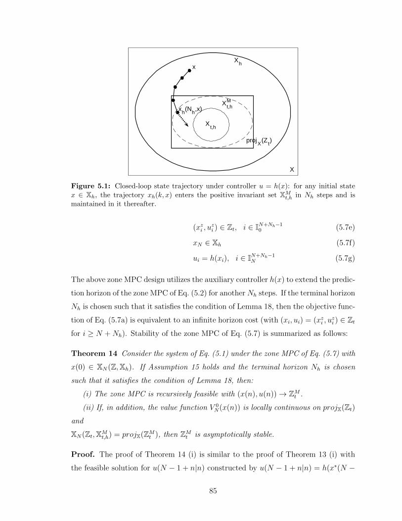
x
xh(N
h,x)
Xt,h
XMt,h
projX
(Zt)
Xh
X
Figure 5.1: Closed-loop state trajectory under controller u = h(x): for any initial statex ∈ Xh, the trajectory xh(k, x) enters the positive invariant set XMt,h in Nh steps and ismaintained in it thereafter.
(xzi , uzi ) ∈ Zt, i ∈ IN+Nh−1
0 (5.7e)
xN ∈ Xh (5.7f)
ui = h(xi), i ∈ IN+Nh−1N (5.7g)
The above zone MPC design utilizes the auxiliary controller h(x) to extend the predic-
tion horizon of the zone MPC of Eq. (5.2) for another Nh steps. If the terminal horizon
Nh is chosen such that it satisfies the condition of Lemma 18, then the objective func-
tion of Eq. (5.7a) is equivalent to an infinite horizon cost (with (xi, ui) = (xzi , uzi ) ∈ Zt
for i ≥ N +Nh). Stability of the zone MPC of Eq. (5.7) is summarized as follows:
Theorem 14 Consider the system of Eq. (5.1) under the zone MPC of Eq. (5.7) with
x(0) ∈ XN(Z,Xh). If Assumption 15 holds and the terminal horizon Nh is chosen
such that it satisfies the condition of Lemma 18, then:
(i) The zone MPC is recursively feasible with (x(n), u(n))→ ZMt .
(ii) If, in addition, the value function V 0N(x(n)) is locally continuous on projX(Zt)
and
XN(Zt,XMt,h) = projX(ZMt ), then ZMt is asymptotically stable.
Proof. The proof of Theorem 14 (i) is similar to the proof of Theorem 13 (i) with
the feasible solution for u(N − 1 + n|n) constructed by u(N − 1 + n|n) = h(x∗(N −
85

1 + n|n − 1)) based on Assumption 15. The proof of Theorem 14 (ii) is similar to
Theorem 13 (ii) with XN(Zt,Xf ) replaced by XN(Zt,XMt,h). The details are omitted
for brevity.
Remark 12 Comparing Theorem 13 (i) and Theorem 14 (i), we can see that the
region of attraction is enlarged from XN(Z,Xf ) to XN(Z,Xh) (because Xf ⊂ Xh).
Moreover, from Theorem 13 (ii) and Theorem 14 (ii), we can see that larger terminal
set Xf or XMt,h is desirable as far as the size of the stability region in the target set is
concerned. We could theoretically use XMt,h as the terminal constraint set Xf in the
zone MPC design of Eq. (5.2). Unfortunately, given the auxiliary controller h(x) and
the target set Zt, the largest positive invariant set XMt,h can be very difficult or compu-
tationally expensive to characterize. Employing the auxiliary controller explicitly in
the zone MPC design as in Eq. (5.7) spares us the burden of explicitly characterizing
XMt,h.
5.5.2 Handling a secondary economic objective
If the optimal solution to the optimization problem of Eq. (5.2) is non-unique, an
economic optimization can be carried out subsequently to make use of the rest degrees
of freedom. Specifically, the optimization problem is formulated as follows:
minui,xzi ,u
zi
N−1∑i=0
l(xi, ui) (5.8a)
s.t. (5.2b)− (5.2f) (5.8b)
N−1∑i=0
|xi − xzi |2Q + |ui − uzi |2R = V 0N(x(n)) (5.8c)
where the cost function l(xi, ui) : Z→ R characterizes process economic performance.
Constraints (5.8b) and (5.8c) confine the solution space of the economic optimization
to be in the solution space of the zone MPC of Eq. (5.2). Therefore the stability
result of Theorem 13 is inherited.
It is also interesting to view the optimization problem of Eq. (5.8) as an economic
MPC (EMPC). In particular, if V 0N(x(M)) = 0 at some time instant M ∈ I≥0, then
86

for all n ≥M , Eq. (5.8) is equivalent to the following EMPC design:
minui
N−1∑i=0
l(xi, ui)
s.t. xi+1 = f(xi, ui), i ∈ IN−10
x0 = x(n)(xi, ui) ∈ Zt, i ∈ IN−1
0
xN ∈ Xf
(5.9)
In the above EMPC optimization problem, the predicted state and input trajectories
are constrained by the target set Zt. Existing EMPC design and analysis methods
(see e.g., [61], [10]) can be applied to the EMPC of Eq. (5.9). For example, one can
find the optimal steady state with respect to the economic cost function l(x, u) in
the target set Zt and verify the dissipativity condition of the optimal steady state
in Zt. Likewise, if the auxiliary controller is utilized in the zone MPC design as
in Eq. (5.7), the corresponding secondary economic optimization problem can be
designed similarly. Existing results of EMPC based on an auxiliary controller [59],
[45] can be applied.
5.6 Examples
Example 1. Consider the following linear scalar system:
x(n+ 1) = 1.25x(n) + u(n)
with state and input constraints X = [−5, 15], U = [−5, 5] respectively. The target
set is Zt = (x, u) | x ∈ [−5, 15], u ∈ [−1, 1]. Using the algorithms in [53] [62],
the largest control invariant set in the target zone can be obtained as follows: ZMt =
(x, u) | Gx+Hu ≤ 1 where G = [0, 0, 0.3125,−0.3125]T , H = [1,−1, 0.25,−0.25]T
(Figure 5.2).
In the simulation, we compare four different zone MPC configurations: (a) a zone
MPC that penalizes the distance to the target set Zt (without terminal constraint),
(b) a zone MPC that penalizes the distance to the largest control invariant set in
the target zone ZMt (also without terminal constraint), (c) the proposed zone MPC
of Eq. (5.2) with Xf = projX(ZMt ) = [−4, 4], and (d) the proposed zone MPC of
Eq. (5.7) with the auxiliary control law h(x) = −0.3x (which asymptotically stabilizes
87
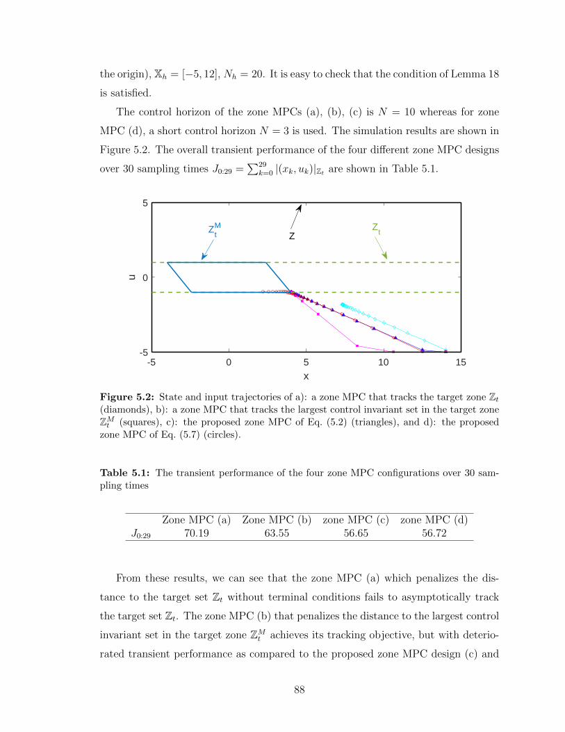
the origin), Xh = [−5, 12], Nh = 20. It is easy to check that the condition of Lemma 18
is satisfied.
The control horizon of the zone MPCs (a), (b), (c) is N = 10 whereas for zone
MPC (d), a short control horizon N = 3 is used. The simulation results are shown in
Figure 5.2. The overall transient performance of the four different zone MPC designs
over 30 sampling times J0:29 =∑29
k=0 |(xk, uk)|Zt are shown in Table 5.1.
-5 0 5 10 15
x
-5
0
5
u
ZtM Z
tZ
Figure 5.2: State and input trajectories of a): a zone MPC that tracks the target zone Zt(diamonds), b): a zone MPC that tracks the largest control invariant set in the target zoneZMt (squares), c): the proposed zone MPC of Eq. (5.2) (triangles), and d): the proposedzone MPC of Eq. (5.7) (circles).
Table 5.1: The transient performance of the four zone MPC configurations over 30 sam-pling times
Zone MPC (a) Zone MPC (b) zone MPC (c) zone MPC (d)J0:29 70.19 63.55 56.65 56.72
From these results, we can see that the zone MPC (a) which penalizes the dis-
tance to the target set Zt without terminal conditions fails to asymptotically track
the target set Zt. The zone MPC (b) that penalizes the distance to the largest control
invariant set in the target zone ZMt achieves its tracking objective, but with deterio-
rated transient performance as compared to the proposed zone MPC design (c) and
88

(d). Moreover, a closer look at the region of attractions of the proposed zone MPC de-
signs (c) and (d) reveals that when N = 3, x(0) /∈ XN(Z,Xf ) and x(0) ∈ XN(Z,Xh).
This indicates that by employing the auxiliary control law in the zone MPC design,
we are allowed to use smaller control horizon N .
It is also worth pointing out that the above results resemble the comparison be-
tween set-point MPC and several popular economic MPC (EMPC) designs [28], [10],
[59]. Specifically, zone MPC (a), (b) corresponds to EMPC without terminal con-
straint and set-point MPC, respectively [10]. Zone MPC (c) corresponds to EMPC
with a point-wise terminal constraint [28]. Zone MPC (d) is analogous to EMPC
with extended horizon based on an auxiliary controller [59].
Example 2. Consider the following nonlinear scalar system:
x(n+ 1) = x(n)2 + u(n) (5.10)
with initial condition x(0) = −1 and input constraint U = [−1.05,−0.95]. The
primary control objective is to maintain the system operation in the target zone:
Zt = (x, u) : x ∈ [−1.5, 0.5], u ∈ [−1.05,−0.95]. There is also a secondary economic
objective to minimize the control input l(x, u) = u. The corresponding optimal steady
state is (xs, us) = (−0.6402,−1.05). We compare two control configurations: (a) a set-
point MPC which tracks (xs, us) (without terminal constraint), and (b) the proposed
zone MPC of Eq. (5.2) which handles the economic objective by taking the second
step economic optimization of Eq. (5.8). The terminal constraint for the zone MPC is
Xf = [−1.5, 0.5]. Both MPCs take the same control horizon N = 5. The simulation
results of cases (a) and (b) are shown in Figure 5.3 and Figure 5.4, respectively.
From Figure 5.3 and Figure 5.4, we can see that set-point MPC achieves its
tracking objective at the expense of making excessive control moves. Note that this
is not because of poor parameter tuning. The zone MPC resulted in a periodic
operation in the target zone. While both MPC designs succeeded in maintaining
the system operation in the target zone, the zone MPC apparently achieves better
transient economic performance.
Further, we compared the performance of set-point MPC and zone MPC in the
presence of small disturbances. An unknown normally distributed process disturbance
w(n) ∼ N (0, 0.1) is introduced to the system: x(n + 1) = x(n)2 + u(n) + w(n).
89

0 10 20 30 40 50 60 70-1.5
-1-0.5
00.5
x
0 10 20 30 40 50 60 70
n
-1.1
-1
-0.9u
Figure 5.3: State and input trajectories of set-point MPC.
0 10 20 30 40 50 60 70-1.5
-1-0.5
00.5
x
0 10 20 30 40 50 60 70
n
-1.05
-1
-0.95
u
Figure 5.4: State and input trajectories of the zone MPC.
0 10 20 30 40 50 60 70-1.5
-1-0.5
00.5
x
0 10 20 30 40 50 60 70
n
-1.05
-1
-0.95
u
Figure 5.5: State and input trajectories of set-point MPC.
90

0 10 20 30 40 50 60 70-1.5
-1-0.5
00.5
x
0 10 20 30 40 50 60 70
n
-1.05
-1
-0.95u
Figure 5.6: State and input trajectories of the zone MPC.
The state and input trajectories of the set-point MPC and zone MPC are shown
in Figure 5.5 and Figure 5.6, respectively. It is seen that in the presence of small
disturbances, zone MPC is still capable of achieving optimal economic performance
while satisfying the zone objective, whereas set-point MPC inevitably suffers from
fluctuations in the control input.
More insights into the superiority of zone control over set-point control can be
acquired by observing the bifurcation diagram in Figure 5.7, which shows the stable
steady states, periodic orbits and chaotic attractors of system (5.10). We can see that
the target zone Zt contains a set of unstable steady states as well as a set of stable
periodic orbits with period 2. Thus, it is clear how relaxing a set-point target to a
zone target can allow for more admissible operations, thereby releasing more degrees
of freedom to achieve economic objectives.
5.7 Summary
In this work, we proposed a general framework of nonlinear model predictive control
for zone tracking. The target zone is characterized by coupled system state and input,
and is not necessarily control invariant. An invariance-like theorem is developed which
naturally generalizes LaSalle’s invariance principle from autonomous system to control
systems with a zone target. Our results differ from the standard stability analysis for
conventional set-point MPC in that we consider the evolvement of the state-input pair
(x(n), u(n)) instead of merely the the state trajectory x(n). This provides stronger
91

Figure 5.7: Bifurcation diagram of system (5.10). The bifurcation diagram shows the thevalues of system state x(n) that are visited or approached asymptotically under a constantu(n). For u ∈ (−0.75,−0.6], the system has stable steady-state operation. At u = −0.75,steady-state operation becomes unstable and the diagram bifurcates into two points whichcorresponds to a stable periodic operation of period two. As the value of u decreases, morebifurcation occurs and at some point around u = −1.4 the system enters a chaotic operatingregion. The dashed line corresponds to steady-state operating points
results and more accurate description of system behavior. Two simulations examples
demonstrate the superiority of zone control over set-point control and the efficacy of
the proposed zone MPC framework.
92

Chapter 6
Application to an Oilsand PrimarySeparation Vessel
In this chapter, we apply the proposed EMPC algorithm to an oilsand primary sep-
aration vessel (PSV). We show how previously developed EMPC design and analysis
results in the context of discrete-time system can be extended to continuous-time
systems where the issue of sampling needs to be addressed. Both infinite-time and
finite-time operations are considered which correspond to the result in Chapter 2 and
Chapter 4.
6.1 Preliminaries
6.1.1 Notation
Throughout this chapter, the operator | · | denotes the Euclidean norm of a scalar
or a vector. A continuous function α : [0, a) → [0,∞) is said to belong to class K
if it is strictly increasing and satisfies α(0) = 0. The symbol Ωr is used to denote a
level set of the Lyapunov function V (x) such that Ωr := x ∈ Rnx : V (x) ≤ r. The
symbol diag(x1, ..., xi, ..., xn) denotes a diagonal matrix with its i-th diagonal element
being xi. The symbol ‘\’ denotes set substraction such that A \B := x ∈ A, x /∈ B.
The operator d·e is used to obtain the smallest integer greater than or equal to a real
number x ∈ R such that dxe := mina ∈ Z : a ≥ x where Z denotes the set of
integers.
93

6.1.2 System description
We consider a class of nonlinear systems which can be described by the following
state-space model:
x(t) = f(x(t)) + g(x(t))u(t) (6.1)
where x ∈ Rnx denotes the state vector and u ∈ Rnu denotes the control input vector.
The control input is restricted to be in a nonempty convex set U ⊂ Rnu , such that:
U := u ∈ Rnu : |u| ≤ umax (6.2)
where umax is the magnitude of the input constraint. It is assumed that f and g are
locally Lipschitz functions with respect to x, and that f(0) = 0 which implies that the
origin is a steady state of the unforced nominal system. We assume that the system
state are sampled periodically at time instants tk≥0 such that tk = t0 + k∆ with
t0 = 0 being the initial time, ∆ being a fixed sampling interval and k being positive
integers.
6.1.3 Stability assumption
We assume that there exists a continuous controller u = h(x) which renders the
origin of system (6.1) asymptotically stable while satisfying the input constraint.
Based on converse Lyapunov theorem [63], the above assumption implies that there
exists a continuous differentiable control Lyapunov function V (x) and K functions
αj, j = 1, 2, 3, 4, that satisfy the following conditions:
α1(|x|) ≤ V (x) ≤ α2(|x|)∂V (x)
∂x
(f(x) + g(x)h(x)
)≤ −α3(|x|)∣∣∣∣∂V (x)
∂x
∣∣∣∣ ≤ α4(|x|)
h(x) ∈ U
(6.3)
for all x ∈ D where D ⊂ Rnx is a compact set containing the origin. We denote a
level set of V (x) in D, Ωρ ⊂ D, as the stability region of the closed-loop system under
the controller h(x).
Using the Lipschitz properties assumed for f , g, and taking into account the
boundedness of the input vector u characterized in Eq. (6.2), there exits a positive
94

constant M such that
|f(x) + g(x)u| ≤M (6.4)
for all x ∈ Ωρ. In addition, by the continuous differentiable property of V (x) and the
Lipschitz properties of f and g, there exist positive constants Lf , Lg, such that:∣∣∣∣∂V (x)∂x
f(x)− ∂V (x′)∂x
f(x′)
∣∣∣∣ ≤ Lf |x− x′|∣∣∣∣∂V (x)∂x
g(x)− ∂V (x′)∂x
g(x′)
∣∣∣∣ ≤ Lg |x− x′|(6.5)
for all x, x′ ∈ Ωρ.
6.2 EMPC with terminal cost
In this section, we present the proposed EMPC with terminal cost and focus on
infinite-time operation. First, we highlight the stability properties of the closed-loop
system under the controller h(x) when it is implemented in a sample-and-hold fashion.
Second, we discuss the design of the terminal cost and then introduce the proposed
EMPC design. Nominal closed-loop stability and asymptotic average performance of
the proposed EMPC design are subsequently analyzed.
6.2.1 Properties of the nonlinear controller h(x)
Since the nonlinear controller h(x) ensures the asymptotic stability of the origin, it
is natural to take advantage of it as the benchmark control system. We are aimed
to develop an EMPC that gives closed-loop economic performance better than (or at
least as good as) the one given by h(x).
In this chapter, we consider that the controller h(x) is implemented in a sample-
and-hold fashion. The sample-and-hold implementation facilitates the construction of
a terminal cost that will be used in the proposed EMPC. When h(x) is implemented
in sample-and-hold, the sampling time ∆ plays an important role in ensuring the
closed-loop stability. If the sampling time is not appropriately picked, the closed-loop
stability under h(x) may be lost. The following proposition summarizes the stability
properties of the controller h(x) implemented in sample-and-hold.
95

Proposition 3 Consider the state trajectory x(t) of the system of Eq. (6.1) in closed-
loop under the controller h(x) implemented in a sample-and-hold fashion with the
initial state x(t0) ∈ Ωρ. If the sampling time ∆ is chosen such that ∆ < ∆max where
∆max ∈ (0,√
ρ(Lf+Lgumax)M
] and is the solution to d(∆max) = 0 with the function d(s)
defined as follows:
d(s) = −α3(α−12 (ρ− (Lf + Lgu
max)Ms2)) + (Lf + Lgumax)Ms (6.6)
with class K functions α2, α3 defined in Eq. (6.3), Lf , Lg defined in Eq. (6.5), and
M defined in Eq. (6.4), then x(t) will be driven into Ωρ∗ ⊂ Ωρ in N∗ steps without
leaving the stability region, where
ρ∗ = α2(α−13 ((Lf + Lgu
max)M∆)) + (Lf + Lgumax)M∆2 (6.7)
and
N∗ =
⌈ρ− ρ∗
−α3(α−12 (ρ∗))∆ + (Lf + Lgumax)M∆2
⌉. (6.8)
Moreover, once x(t) enters Ωρ∗, it is maintained in it thereafter.
Proof. First, we show that ∆max that satisfies Eq. (6.6) uniquely exists. It can
be verified that d(s) is a strictly increasing function for s ∈ [0,√
ρ(Lf+Lgumax)M
]. It
can also be easily checked that d(0) < 0 and d(√
ρ(Lf+Lgumax)M
) > 0. Therefore the
∆max that satisfies d(∆max) = 0 for ∆max ∈ (0,√
ρ(Lf+Lgumax)M
] uniquely exists.
Second, we show that when ∆ ≤ ∆max, the stability conditions established in [64]
are satisfied and the system state will be driven into Ωρ∗ in N∗ steps and is maintained
in it thereafter. Note first that ρ∗ < ρ holds automatically which can be verified from
the definition of ∆max and the fact that ∆ < ∆max. From Eq. (6.7), the following
inequality holds:
−α3(α−12 (ρ∗)) + (Lf + Lgu
max)M∆ < 0 (6.9)
From the analysis in [64], the above equation implies that
V (x(t)) < −α3(α−12 (ρ∗)) + (Lf + Lgu
max)M∆, ∀ x(t) ∈ Ωρ \ Ωρ∗ (6.10)
which further implies that any x(t0) ∈ Ωρ \Ωρ∗ will be driven into Ωρ∗ in less than N∗
steps while V (x) keeps decreasing. To show that once x enters Ωρ∗ it is maintained in
96

it thereafter, we note that for any ρs ∈ (ρo, ρ], where ρo = α2(α−13 ((Lf+Lgu
max)M∆)),
the following inequality holds
−α3(α−12 (ρs)) + (Lf + Lgu
max)M∆ < 0 (6.11)
Using the result in [64] again, the above inequality implies that x is ultimately main-
tained in Ωρ∗o , where ρ∗o := maxV (x(t + ∆)) : V (x(t)) ≤ ρo. Further, for any
x(tk) ∈ Ωρo , the change rate of the Lyapunov function V (x) is bounded as follows for
t ∈ [tk, tk+1]:
V (t) < −α3(α−11 (ρo)) + (Lf + Lgu
max)M∆ < (Lf + Lgumax)M∆ (6.12)
Taking into account the definition of ρ∗o and the above inequality, the following upper
bound on ρ∗o can be obtained:
ρ∗o < ρo + (Lf + Lgumax)M∆2 = ρ∗ (6.13)
which means that x is ultimately maintained in Ωρ∗
It can be seen from Proposition 3 that the nonlinear controller h(x) implemented
in sample-and-hold is capable of maintaining system state inside the stability region
if the sampling time ∆ is sufficiently small. Moreover, it will drive the system state
into a level set Ωρ∗ ⊂ Ωρ in N∗ steps. Note that ρ∗ and N∗ are both monotonic
functions of ∆ for ∆ ∈ (0,∆max). Smaller sampling time ∆ results in smaller ρ∗ and
larger N∗. Moreover, arbitrarily small ρ∗ can be obtained if the sampling time ∆ can
be made arbitrarily small.
Remark 13 Note that the stability property of h(x) implemented in sample-and-hold
in Proposition 3 is made possible due to the continuous differentiability of the Lya-
punov function V (x) as well as the Lipschitz properties of f and g. Note also that the
result in Proposition 3 is conservative in the sense that the actual region in which x is
maintained after N∗ steps might be much smaller than Ωρ∗ characterized by Eq. (6.7)
because worst case is assumed throughout the analysis.
6.2.2 Proposed EMPC design
To proceed, we define x(t|tk) and u(t|tk) as the predicted state and input trajecto-
ries of the system of Eq. (6.1) under the sample-and-hold implementation of h(x)
97

evaluated at tk with the initial condition x(tk|tk) = x(tk). Specifically, for a time
interval t ∈ [tk, tk+Nh ], the predicted state and input trajectories can be obtained by
integrating the following differential equation recursively for l = 0, ..., Nh − 1:
˙x(t|tk) = f(x(t|tk)) + g(x(t|tk))u(t|tk), t ∈ [tk+l, tk+l+1) (6.14a)
u(t|tk) = h(x(tk+l|tk)), t ∈ [tk+l, tk+l+1) (6.14b)
x(tk|tk) = x(tk) (6.14c)
A function, c(x(tk), Nh), that characterizes the accumulated economic performance
of the nominal system under h(x) implemented in sample-and-hold over Nh sampling
periods with the initial state x(tk|tk) = x(tk) can thus be defined as follows:
c(x(tk), Nh) =
∫ tk+Nh
tk
l(x(t|tk), u(t|tk))dt (6.15)
where l(x, u) is a bounded function defined on (x, u) : x ∈ Ωρ, u ∈ U that charac-
terizes the dynamic economic cost of the system at a specific time instant.
In the proposed design, EMPC minimizes the economic cost function l(x, u) for a
prediction horizon of N sampling periods with the cost function c(x,Nh) incorporated
as the terminal cost. The system state is allowed to be operated only in the stability
region Ωρ. Specifically, the proposed EMPC at a sampling time tk is formulated as
the following optimization problem:
minu(τ)∈S(∆)
∫ tk+N
tk
l(x(τ), u(τ))dτ + c(x(tk+N), Nh) (6.16a)
s.t. ˙x(t) = f(x(t)) + g(x(t))u(t) (6.16b)
x(tk) = x(tk) (6.16c)
u(t) ∈ U (6.16d)
x(t) ∈ Ωρ (6.16e)
where S(∆) denotes the family of continuous piece-wise functions with sampling time
∆ and x denotes the predicted state trajectory in this optimization problem.
In the above optimization problem, Eq. (6.16a) is the objective function involving
the accumulated economic performance over the prediction horizon (i.e., the first
term in the objective function) and a terminal cost c(x(tk+N), Nh). Eq. (6.16b) is the
system model. Eq. (6.16c) specifies the initial condition at time tk. Eq. (6.16d) is
98

the constraint on control input u. Eq. (6.16e) specifies the region in which EMPC is
allowed to operate which is used to ensure the closed-loop stability of the proposed
EMPC.
The optimal solution to the optimization problem of Eq. (6.16) is denoted as
u∗(t|tk), t ∈ [tk, tk+N), with the corresponding optimal state trajectory denoted as
x∗(t|tk), t ∈ [tk, tk+N). The manipulated input of the closed-loop system under the
proposed EMPC at a sampling instant tk is defined as follows:
u(t) = u∗(t|tk), t ∈ [tk, tk+1) (6.17)
which is the first value of the optimal input sequence. At the next sampling instant
tk+1, the optimization problem of Eq. (6.16) is re-evaluated.
6.2.3 Stability and performance analysis
In this subsection, we analyze the stability and economic performance of the system
under the proposed EMPC design of Eq. (6.16). The stability property of the proposed
EMPC design is presented in the following theorem.
Theorem 15 Consider the system of Eq. (6.1) in closed-loop under the proposed
EMPC design of Eq. (6.16) with the initial state x(t0) ∈ Ωρ. If the sampling time ∆
satisfies ∆ < ∆max, then the optimization problem is feasible for all tk ≥ t0, and the
system state x(t) ∈ Ωρ for all t ≥ t0.
Proof. We use induction to prove this theorem. At a sampling time tk, let us assume
that x(tk) ∈ Ωρ. If the sampling time ∆ satisfies ∆ < ∆max, it can be obtained from
Proposition 1 that the predicted trajectory x(t|tk) following Eq. (6.15) with Nh = N
is maintained in Ωρ for t ∈ [tk, tk+N) (i.e., constraint (6.16e) is satisfied). Also, the
corresponding u(t|tk) for t ∈ [tk, tk+N) satisfies the input constraint (6.16d). This
implies that the optimization problem of Eq. (6.16) is feasible at tk. Moreover, the
feasibility of the optimization problem of Eq. (6.16) at tk implies that x(t) ∈ Ωρ for
t ∈ [tk, tk+1] since the first step input value is the actual input applied to the system.
x(tk+1) ∈ Ωρ further implies that the optimization problem of Eq. (6.16) at tk+1 is
also feasible. If x(t0) ∈ Ωρ, following the reasoning of induction, the optimization
99

problem of Eq. (6.16) is feasible for all tk ≥ t0, and x(t) ∈ Ωρ for all t ≥ t0. This
proves Theorem 15.
Next, we analyze the closed-loop economic performance of the proposed EMPC. In
particular, we focus on the asymptotic average economic performance since infinite-
time operation is considered. The asymptotic average economic performance is de-
fined as follows:
Jasy := limF→∞
1
F∆
∫ tF
t0
l(x(t), u(t))dt (6.18)
Theorem 2 below provides an upper bound on the asymptotical average performance
of the proposed EMPC design.
Theorem 16 Consider the system of Eq. (6.1) in closed-loop under the proposed
EMPC design of Eq. (6.16) with the initial state x(t0) ∈ Ωρ and sampling time
∆ < ∆max. If Nh is chosen such that Nh ≥ N∗, then the asymptotical average eco-
nomic performance of the closed-loop system under the EMPC, JEMPCasy , is bounded
as follows:
JEMPCasy ≤ Jh∆ (6.19)
where
Jh∆ := max
1
∆
∫ ∆
0
l(x(t), h(x(0)))dt : x(0) ∈ Ωρ∗
(6.20)
which denotes the maximum possible average economic performance over one sampling
period ∆ under the nonlinear controller h(x) implemented in sample-and-hold when
the closed-loop system state is within Ωρ∗.
Proof. Let us use L(tk) to denote the objective function value of the optimization
problem of Eq. (6.16) evaluated at sampling time tk. L(tk) corresponds to the accumu-
lated economic performance of the open-loop system under the following augmented
input sequence implemented in sample-and-hold for t ∈ [tk, tk+N+Nh ]:
U∗(tk) = [u∗(tk|tk), ..., u∗(tk+N−1|tk), h(x(tk+N |tk+N)), ..., h(x(tk+N+Nh−1|tk+N))]
(6.21)
where x(t|tk+N) for t ∈ [tk+N , tk+N+Nh ] denotes the predicted state trajectory under
the nonlinear controller h(x) implemented in sample-and-hold starting from x∗(tk+N |tk).
We will refer to U∗(tk) as the optimal augmented solution to the optimization problem
of Eq. (6.16) at tk.
100

Since x∗(tk+N |tk) ∈ Ωρ (due to Eq. (6.16e)) and Nh ≥ N∗, from Proposition 3,
it can be obtained that the augmented optimal input sequence U∗(tk) will drive the
predicted state trajectory into the invariant set Ωρ∗ , that is:
x(tk+N+Nh |tk+N) ∈ Ωρ∗ (6.22)
Let us further construct the following augmented input sequence:
U(tk+1) = [u∗(tk+1|tk), ..., u∗(tk+N−1|tk), h(x(tk+N |tk+N)), ..., h(x(tk+N+Nh|tk+N))]
(6.23)
which is obtained by discarding the first value in U∗(tk) and applying h(x) for one
more step at the end. It can be shown that U(tk+1) is a feasible augmented solution
to the optimization problem of Eq. (6.16) at tk+1. To verify this, we only need
to check whether h(x(tk+N |tk+N)) satisfies the input constraint of Eq. (6.16d) and
whether the state trajectory x(t|tk+N) for t ∈ [tk+N , tk+N+1] satisfies the constraint
of Eq. (6.16e). Both of these can be verified based on the properties of h(x) and the
fact that x∗(tk+N |tk) ∈ Ωρ.
Let L(tk+1) denote the objective function corresponding to U(tk+1). From the
definition of U(tk+1), L(tk+1) can be expressed as follows:
L(tk+1) = L(tk)−∫ tk+1
tkl(x∗(t|tk), u∗(tk|tk))dt
+∫ tk+N+Nh+1
tk+N+Nh
l(x(t|tk+N), h(x(tk+N+Nh|tk+N))dt(6.24)
Since u∗(tk|tk) is the actually implemented control input, the second term of the right-
hand-side of the above equation can be replaced with the economic performance of
the actual state and input trajectories∫ tk+1
tk
l(x∗(t|tk), u∗(tk|tk))dt =
∫ tk+1
tk
l(x(t), u(t))dt. (6.25)
Moreover, taking into account the definition of Jh∆ and the fact that x(tk+N+Nh|tk+N) ∈
Ωρ∗ , the following inequality holds:∫ tk+N+Nh+1
tk+N+Nh
l(x(t|tk+N), h(x(tk+N+Nh|tk+N))dt ≤ Jh∆∆ (6.26)
Substituting Eq. (6.25) and Eq. (6.26) into Eq. (6.24), the following inequality can
be obtained:
L(tk+1) ≤ L(tk)−∫ tk+1
tk
l(x(t), u(t))dt+ Jh∆∆ (6.27)
101

The principle of optimality indicates that L(tk+1) ≤ L(tk+1), which gives:
L(tk+1) ≤ L(tk)−∫ tk+1
tk
l(x(t), u(t))dt+ Jh∆∆ (6.28)
Summing the above inequality from k = 0 to F − 1 on both sides and combining the
integration terms, the following inequality can be obtained:∫ tF
t0
l(x(τ), u(τ))dτ ≤ L(t0)− L(tF ) + Jh∆F∆ (6.29)
Dividing F∆ on both sides with F approaching infinity, and taking into account
that L(tk) at any specific sampling instant is a finite value because it is a finite time
integration of the bounded cost function l(x, u), the following inequality is obtained:
JEMPCasy = lim
F→∞
1
F∆
∫ tF
t0
l(x(τ), u(τ))dτ ≤ limF→∞
L(t0)− L(tF )
F∆+ Jh∆ = Jh∆ (6.30)
This proves Theorem 16.
Remark 14 In Theorem 16, Jh∆ characterizes the worst possible average economic
performance over one sampling period ∆ that may be obtained when h(x) is imple-
mented in sample-and-hold and the system state is inside the invariant set Ωρ∗. When
the region Ωρ∗ is sufficiently small, if we further assume that the performance metric
l(x, u) is smooth, it is expected that different trajectories in Ωρ∗ will give approximately
the same economic performance. This further implies that:
Jh∆ ≈ limF→∞
1
F∆
∫ F∆
0
l(x, h)dt (6.31)
where x(0) ∈ Ωρ∗. Since h is able to drive the state to Ωρ∗, the above approxima-
tion (6.31) also holds when x(0) ∈ Ωρ. This implies that:
Jh∆ ≈ Jhasy (6.32)
for x(0) ∈ Ωρ. Therefore, the statement in Theorem 1 may also implies that the
asymptotic average performance of the proposed LEMPC is no worse than the asymp-
totic average performance of the controller h.
102

6.3 Fixed-time implementation
In the previous section, a terminal cost EMPC based on the auxiliary controller h(x)
is proposed in which the terminal cost c(x,Nh) is predetermined. It is shown that the
proposed terminal cost EMPC achieves guaranteed asymptotical average performance
over infinite time operation. In this section, we focus on finite-time operation. We
propose an revised implementation strategy of the proposed EMPC with terminal
cost that achieves improved economic performance over the auxiliary controller h(x)
implemented in sample-and-hold for a fixed time duration longer than the prediction
horizon.
6.3.1 Implementation strategy
We consider the performance of the EMPC in a fixed time interval [t0, tF ] where
F > N . The proposed fixed-time EMPC implementation consists of two stages.
In the first stage when tk ∈ [t0, tF−N ], the proposed EMPC design of Eq. (6.16) is
implemented with Nh shrinking every sampling time from F −N to 0; in the second
stage when tk ∈ [tF−N+1, tF ] the proposed EMPC design of Eq. (6.16) is implemented
with Nh = 0 and the prediction horizon shrinking every sampling time from N to 0.
The specific EMPC formulations at the two stages are as follows:
Stage 1 : At a sampling instant tk, tk ∈ [t0, tF−N ], the proposed EMPC design is
formulated as follows:
minu(τ)∈S(∆)
∫ tk+N
tk
l(x(τ), u(τ))dτ + c(x(tk+N), F − k −N) (6.33a)
s.t. ˙x(τ) = f(x(τ)) + g(x(τ))u(τ) (6.33b)
x(tk) = x(tk) (6.33c)
u(τ) ∈ U (6.33d)
x(τ) ∈ Ωρ (6.33e)
The first step value of the optimal solution to the optimization problem of Eq. (6.33) is
implemented between tk and tk+1. At the next sampling instant tk+1, the optimization
problem of Eq. (6.33) is re-evaluated until tk = tF−N .
103

Stage 2 : At a sampling instant tk, tk ∈ [tF−N+1, tF ], the proposed EMPC design
is formulated as follows:
minu(τ)∈S(∆)
∫ tF
tk
l(x(τ), u(τ))dτ (6.34a)
s.t. ˙x(τ) = f(x(τ)) + g(x(τ))u(τ) (6.34b)
x(tk) = x(tk) (6.34c)
u(τ) ∈ U (6.34d)
x(τ) ∈ Ωρ (6.34e)
Again, the first step value of the optimal solution to the optimization problem of Eq.
(6.34) is implemented. At the next sampling instant tk+1, the optimization problem
of Eq. (6.34) is re-evaluated until tk = tF .
6.3.2 Stability and performance analysis
In this subsection, we analyze the stability and economic performance of the proposed
fixed-time EMPC implementation. The stability property of the fixed-time EMPC
implementation is presented in the following theorem.
Theorem 17 Consider the system of Eq. (6.1) in closed-loop under the fixed-time
EMPC implementation of Eq. (6.33) and Eq. (6.34) with the initial state x(t0) ∈ Ωρ.
If the sampling time ∆ satisfies ∆ < ∆max, then the optimization problems are feasible
for all tk ∈ [t0, tF ], and the system state x(t) ∈ Ωρ for all t ∈ [t0, tF ].
Proof. The fixed-time EMPC designs of Eq. (6.33) and Eq. (6.34) are in the same
form of the EMPC of Eq. (6.16). Following similar arguments as in the proof of The-
orem 15, the closed-loop stability of the proposed fixed-time EMPC implementation
can be proved.
The economic performance of the fixed-time EMPC implementation is summarized
in Theorem 18 below.
Theorem 18 Consider the accumulated closed-loop economic performance of the sys-
tem of Eq. (6.1) for a fixed time interval [t0, tF ], with the initial state x(t0) ∈ Ωρ and
sampling time ∆ < ∆max. The accumulated economic performance of the closed-loop
104
system under the fixed-time EMPC implementation of Eq. (6.33) and Eq. (6.34) is
no worse than the accumulated economic performance of the closed-loop system under
h(x) implemented in sample-and-hold; that is:∫ tF
t0
l(x(t), u(t))dt ≤ c(x(t0), F ) (6.35)
where x and u are the actual optimal state and input trajectories under the proposed
fixed-time EMPC implementation strategy.
Proof. Let us use L(tk) to denote the objective function value of the optimization
problem of Eq. (6.33) or Eq. (6.34) evaluated at sampling time tk. L(tk) corresponds
to the accumulated economic performance of the open-loop predicted system state
trajectory under the following input or augmented input sequence implemented in
sample-and-hold for t ∈ [tk, tF ]:
U∗(tk) = [u∗(tk|tk), ..., u∗(tF−1|tk)]. (6.36)
Note that when tk ≤ tF−N , U∗(tk) for the optimization problem of Eq. (6.33) in stage
1 is the optimal augmented input sequence as follows:
U∗(tk) = [u∗(tk|tk), ..., u∗(tk+N−1|tk), h(x(tk+N |tk+N)), ..., h(x(tk+F−1|tk+N))] (6.37)
It can be easily verified that the input sequence U(tk+1) = [u∗(tk+1|tk), ..., u∗(tF−1|tk)]
is a feasible solution to the EMPC optimization problems at tk+1. The objective func-
tion corresponding to this input sequence can be expressed as follows:
L(tk+1) = L(tk)−∫ tk+1
tk
l(x(t), u(t))dt (6.38)
The principle of optimality indicates that L(tk+1) ≤ L(tk+1), which gives:
L(tk+1) ≤ L(tk)−∫ tk+1
tk
l(x(t), u(t))dt (6.39)
Summing the above inequality from k = 0 to F − 1 on both sides and combining the
integration terms, the following inequality can be obtained:∫ tF
t0
l(x(τ), u(τ))dτ ≤ L(t0)− L(tF ) (6.40)
105

At the sampling time tF ,
L(tF ) =
∫ tF
tF
l(x(τ), u(τ))dτ = 0 (6.41)
Because the input sequence generated by h(x) in sample-and-hold from t0 to tF−1 with
initial state x(t0) ∈ ρ is a feasible augmented solution to the optimization problem of
Eq. (6.33) at t0 , the following inequality holds:
L(t0) ≤ c(x(t0), F ) (6.42)
Substituting Eq. (6.41) and Eq. (6.42) into Eq. (6.40):∫ tF
t0
l(x(t), u(t))dt ≤ c(x(t0), F ) (6.43)
This proves Theorem 18.
Remark 15 We note that the shrinking horizon approach as used in Stage 2 may
be used directly starting from t0 with the initial horizon N = F and the results in
Theorem 18 still hold. Similar ideas have been used in [65, 30] to ensure finite-time
performance of EMPC. However, the computational demand of such an implemen-
tation could be very high or even prohibitive for online implementation especially
when F is very large. Taking advantage of the terminal cost, the proposed fixed-time
EMPC implementation is capable of achieving improved fixed-time performance over
the auxiliary controller h(x) with any predetermined prediction horizon N which is
an appealing feature for online implementation.
Remark 16 At the second stage of the proposed fixed-time implementation strategy,
the system state trajectory may be governed by the Turnpike property [66]. In this
case, the system state will deviate from the steady state at the end of the fixed time
window. An alternative implementation strategy to circumvent the dramatic deviation
is to implement the auxiliary controller h(x) instead of the shrinking horizon EMPC
at stage 2. If h(x) is implemented at stage 2, the stability and performance analysis in
Theorem 17 and Theorem 18 still hold. This implementation strategy will be compared
with the strategy outlined in Section 6.3.1 in Section 6.4.
106

6.4 Application to a primary separation vessel
6.4.1 Process description and modeling
The primary separation vessel (PSV) is a key unit in the Clark hot water extraction
process which is used for extraction of all commercial minable oil sands. As the first
step in the extraction process, PSV facilitates the separation of aerated bitumen and
coarse solid particles (clay, sand, etc.). Figure 6.1 shows a schematic of the PSV
process. Oilsand ore is first fed into a mixing tank in which it is mixed with flood
Figure 6.1: Schematic of the primary separation vessel
water, air and other process additives. The mixed oilsand slurry is then fed into
the middle of the primary separation vessel in which gravity separation takes place
due to the density difference of bitumen droplets, water and solids. A bitumen rich
stream (froth) is withdrawn on top of the vessel and sent to downstream units for
further processing. There are also streams withdrawn from the middle and the bottom
layers. The stream withdrawn from the middle layer primarily contains water while
the stream from the bottom layer mostly contains solids.
In the PSV process model, we assume that there are three typical bitumen parti-
cles and three solid particles in the feed stream. The mixer is modeled as a continuous
stirred tank. The separation vessel is modeled into three distinguishable layers: top
froth, middlings and tailings [67]. Each layer is assumed to be well mixed and all com-
position densities are considered constant. The froth/middlings interface level, which
is a crucial control index [68], is dynamically modeled. The middlings/tailings inter-
face is assumed to be stationary (i.e., volume of the tailings layer is constant). Based
107

on mass balance and standard modeling assumptions, a set of ordinary differential
equations is derived to describe the dynamics of the system [67]:
dαfdbjdt
=1
Vmix(Qore(α
orebj − α
fdbj )−Qflα
fdbj ) (6.44a)
dαfdsjdt
=1
Vmix(Qore(α
oresj − α
fdsj )−Qflα
fdsj ) (6.44b)
dVfdt
= vIA (6.44c)
dαfbjdt
=
1Vf
(−αmbjvmbjA+ vIA(αmbj − αfbj)−Qfα
fbj), if vmbj − vI < 0
1Vf
(−αfbjvmbjA−Qfαfbj), if vmbj − vI ≥ 0
(6.44d)
dαfsjdt
=
1Vf
(−αmsjvmsjA+ vIA(αmsj − αfsj)−Qfα
fsj), if vmsj − vI < 0
1Vf
(−αfsjvmsjA−Qfαfsj), if vmsj − vI ≥ 0
(6.44e)
dαmbjdt
=
1Vm
(Qfdαfdbj −Qmα
mbj − αmbjvtbjA+ αmbjv
mbjA), vmbj − vI < 0
1Vm
(Qfdαfdbj −Qmα
mbj − αmbjvtbjA+ αfbjv
mbjA+ vIA(αmbj − α
fbj)), vmbj − vI ≥ 0
(6.44f)
dαmsjdt
=
1Vm
(Qfdαfdsj −Qmα
msj − αmsjvtsjA+ αmsjv
msjA), vmsj − vI < 0
1Vm
((Qfdαfdsj −Qmα
msj − αmsjvtsjA+ αfsjv
msjA+ vIA(αmsj − α
fsj)), vmsj − vI ≥ 0
(6.44g)
dαtbjdt
=1
Vt(αmbjv
tbjA−Qtα
tbj) (6.44h)
dαtsjdt
=1
Vt(αmsjv
tsjA−Qtα
tsj) (6.44i)
where j = 1, 2, 3 stands for the j-th species of bitumen or solids. The definition
of model variables are given in Table 6.1. The values of constant model parameters
are given in Table 6.2. In this model, the movement of all particles is assumed to
be one-dimensional with the downward direction taken as the positive direction. The
volumes of each layers satisfy:
Vm + Vf + Vt − V = 0 (6.45)
The volumetric flows satisfy the following volume balance equations:
Qore +Qfl = Qfd = Qf +Qm +Qt (6.46)
The relative slip velocities of the particles are calculated using the following hindered
108

settling model [69] :
vibj =gd2
bjF (αiw)(ρbj − ρi)18µw
(6.47a)
visj =gd2
sjF (αiw)(ρsj − ρi)18µw
(6.47b)
where i = f, m, t, stands for the froth layer, middlings layer and tailings layer,
respectively. The function F (αiw) is the Barnea and Mizrachi correlation [70]:
F (αiw) = [1 + (1− αiw)13 e
5(1−αiw)
3αiw ]−1 (6.48)
The volumetric fraction of water in layer i, i = f, m, t, satisfies the overall volume
balance in layer i:
αiw = 1−3∑j=1
αibj −3∑j=1
αisj (6.49)
The suspension in layer i, i = f, m, t, is assumed to be uniform and its density is
calculated as the weighted summation of component densities:
ρi = ρwαiw +
3∑j=1
ρbjαibj +
3∑j=1
ρsjαisj (6.50)
The froth/middlings interface velocity, vI , is modeled by first order approximation of
the shockwave equation [71]:
vI =
3∑j=1
αmbjvmbj −
3∑j=1
αfbjvfbj
3∑j=1
αmbj −3∑j=1
αfbj
(6.51)
6.4.2 EMPC design
The system state vector which includes the volume of froth layer and the volumet-
ric concentrations of all bitumen and solid species of the feed stream, froth layer,
middlings layer and tailings layer, is defined as follows:
x = [ Vf αfdb1 αfdb2 αfdb3 αfds1 αfds2 αfds3 αfb1 αfb2 αfb3 αfs1 αfs2 αfs3αmb1 αmb2 αmb3 αms1 αms2 αms3 αtb1 αtb2 αtb3 αts1 αts2 αts3 ]T
(6.52)
109

Table 6.1: Process variables.
Qore, Qfl, Qfd, Qf , Qm, Qt volumetric flow rates of the oilsand ore, flood water,feed stream, froth stream, middlings stream andtailings stream
V, Vf , Vm, Vt, Vmix volumes of the vessel, froth layer, middlings layer,tailings layer and the feed flow mixer
A cross section area of the vesselvI froth/middlings interface velocity
αfdbj , αfbj, α
mbj , α
tbj volumetric fractions of the j-th bitumen in feed
stream, froth layer, middlings layer and tailingslayer
αfdsj , αfsj, α
msj, α
tsj volumetric fractions of the j-th solid in feed stream,
froth layer, middlings layer and tailings layerαfdw , α
fw, α
mw , α
tw volumetric fractions of water in feed stream, froth
layer, middlings layer and tailings layerαorebj , α
oresj volumetric fractions of the j-th bitumen and sands
in the ore
vfbj, vmbj , v
tbj slip velocities of the j-th bitumen in froth layer,
middlings layer and tailings layer
vfsj, vmsj , v
tsj slip velocities of the j-th solid in froth layer, mid-
dlings layer and tailings layerρbj, ρsj, ρw the j-th bitumen particle, j-th solid particle and
water densitiesdbj, dsj the j-th bitumen particle and solid particle diame-
tersρf , ρm, ρt suspension densities of froth layer, middlings layer
and tailings layerµw viscosity of waterg gravitation costant
110

Table 6.2: Model parameters.
ρb = [800, 750, 700] kg/m3 A = 8.5 m2
ρs = 2650 kg/m3 µw = 3.25× 10⁻⁴ kg/(m · s)ρw = 971.8 kg/m3 g = 9.81m/s2
αoreb = [0.021, 0.038, 0.051] db = [2.8, 5.8, 7.0]× 10−5 mαores = [0.0168, 0.042, 0.630] ds = [0.78, 1.311, 12.5]× 10−5 mV = 1000 m3 Vt = 200 m3
Vmix = 4.15 m3 Qore = 0.0056m3/s
Table 6.3: Steady-state operating point.
αfdb = [0.0075, 0.0136, 0.0183] αfds = [0.0603, 0.0151, 0.2262]
αfb = [0.0648, 0.2019, 0.2918] αfs = [0, 0, 0]αmb = [0.0232, 0.0159, 0.0149] αms = [0.2982, 0.0598, 0.0315]αtb = [0, 0, 0] αts = [0.0106, 0.0060, 0.2861]Qfl = 0.0100 m3/s Qf = 0.0008m3/sQm = 0.0027 m3/s Qt = 0.0120m3/sVf = 200.0 m3
The input vector which includes flow rates of flood water, middlings stream and
tailings stream, is defined as follows:
u = [u1 u2 u3]T = [Qfl Qm Qt]T (6.53)
The economic objective of the PSV process is to maximize the overall recovery rate
of bitumen from feed ore, which is equivalent to minimizing the time integration of
the following function:
r(x(t), u(t)) = −∑3
j=1 αfbj(t)Qf (t)∑3
j=1 αorebj Qore
= −(x8(t) + x9(t) + x10(t)
)(Qore + u1(t)− u2(t)− u3(t)
)∑3j=1 α
orebj Qore
(6.54)
111

The optimal steady state operating point is obtained by solving the following steady-
state optimization problem:
(xs, us) = arg min r(x, u)
s.t. f(x) = 0
u ∈ U(6.55)
where f(x) is the right-hand-side of the process model of Eq. (6.44) and the control
input is bounded inside the convex set U defined as follows:
U :=
(u1, u2, u3) :
0 ≤ u1 ≤ 0.01
0 ≤ u2 ≤ 0.03
0 ≤ u3 ≤ 0.03
Qf = Qore + u1 − u2 − u3 ≥ 0
(6.56)
The obtained optimal steady state is shown in Table 6.3. The economic cost function
of EMPC is defined as follows:
l(x, u) = r(x, u) + d(u) (6.57)
where the term d(u(t)) penalizes the incremental of the inputs and is defined as
follows:
d(u(t)) = |u(t)− u(tk−1)|2R, t ∈ (tk−1, tk] (6.58)
where R = diag(104, 104, 104). The incremental penalty term d(u(t)) is incorporated
into the economic cost function to make the optimal solution unique while not chang-
ing the optimal steady state. The nonlinear auxiliary controller h(x) is chosen as a
single proportional controller paired between the froth volume Vf and the middling
outlet flow rate Qm, specifically:
h(x) = [u1s, u2s + p(x1 − x1s), u3s]T (6.59)
where the proportional gain is p = −10−7. A quadratic Lyapunov function:
V (x) = (x− xs)TP (x− xs) (6.60)
with P = diag(10−4, 1, 1, ..., 1) is used. A ρ = 0.2 level set of the quadratic Lyapunov
function is chosen as the stability region in which the system state is allowed to
evolve. The corresponding operating region for the froth layer volume is 155.3m3 <
112

Table 6.4: Transient and steady-state average bitumen recovery rates of the closed-loopsystem under the proposed EMPC with terminal cost, the EMPC in [1], the tracking MPCand the controller h(x)
Proposed EMPC EMPC in [1] Tracking MPC h(x)Transient average 0.8816 0.8123 0.7754 0.7690
Steady state 0.7514 0.7389 0.7611 0.7611
Vf < 244.7m3. The sampling time is ∆ = 1 h, the prediction horizon is N = 5, and
the terminal cost evaluation step is Nh = 30.
In addition, the proposed EMPC design will be compared with the conventional
tracking MPC. The stage cost of the tracking MPC is lt(x, u) = |x− xs|2Q + |u− us|2Rwhere the weighting matrices areQ = diag(10−4, 1, 1, ..., 1) andR = diag(104, 104, 104).
6.4.3 Simulation result
In this subsection, the performance of the proposed EMPC design will be compared
with 1) an EMPC without terminal cost [1], 2) the conventional tracking MPC and
3) the controller h(x). The initial state of all simulation runs is:
x(0) = [190.0 0.0516 0.2106 0.3225 0 0 0 0.0168 0.0151
0.0151 0.1865 0.0459 0.2179 0 0 0 0.0020 0.0014
0.6097 0.0122 0.0220 0.0296 0.0975 0.0244 0.3656 ]T
(6.61)
We first compare the performance of the proposed EMPC with terminal cost
for infinite-time operation with the other control configurations. The closed-loop
bitumen recovery rate trajectories, r(x(t), u(t)), under different controllers are shown
in Fig. 6.2. The closed-loop froth layer volume trajectories are shown in Fig. 6.3.
The closed-loop trajectories of the quadratic Lyapunov function of Eq. (6.60), which
indicate the overall state evolutions, are shown in Fig. 6.4. The closed-loop input
trajectories are shown in Fig. 6.5. The transient average recover rate for t ∈ [0, 72h]
and the steady state recovery rates achieved by different controllers are shown in
Table 6.4.
From these results, it can be seen that the controller h(x) and the tracking MPC
eventually drive the system state to the optimal steady state. The two EMPC config-
113

0 20 40 60 720
2
4
t (h)
r
Figure 6.2: Bitumen recovery rate trajectores of the closed-loop system under the proposedEMPC with terminal cost (dashed line), the EMPC in [1] (dotted line), the tracking MPC(dash dotted line) and the controller h(x) (solid line).
0 20 40 60 72165
175
185
195
205
210
t (h)
Vf (
m3 )
Figure 6.3: Froth layer volume trajectores of the closed-loop system under the proposedEMPC with terminal cost (dashed line), the EMPC in [1] (dotted line), the tracking MPC(dash dotted line) and the controller h(x) (solid line).
114

0 20 40 60 720
0.05
0.1
0.15
0.2
t (h)
V(x
)
Figure 6.4: Lyapunov function trajectores of the closed-loop system under the proposedEMPC with terminal cost (dashed line), the EMPC in [1] (dotted line), the tracking MPC(dash dotted line) and the controller h(x) (solid line).
0 10 20 30 40 50 60 700
2
4x 10
−3
Qm
(m
3 /s)
0 10 20 30 40 50 60 700.005
0.01
0.015
Qt (
m3 /s
)
t (h)
0 10 20 30 40 50 60 706
8
10x 10
−3
Qfl (
m3 /s
)
Figure 6.5: Input trajectories of the closed-loop system under the proposed EMPC withterminal cost (dashed line), the EMPC in [1] (dotted line), the tracking MPC (dash dottedline) and the controller h(x) (solid line).
115

Table 6.5: Average bitumen recovery rates of the closed-loop system under (a): theinfinite-time implementation, (b): fixed-time implementation, (c): alternative fixed-timeimplementation, and (d): the controller h(x).
(a) (b) (c) (d)Average recovery rate 0.8816 1.0191 0.8798 0.7690
urations (with and without terminal cost) drive the system state to new steady states
slightly different from the optimal steady state while maintaining the system state
inside the stability region. Note that this result agrees with the performance analysis
in Theorem 2. It can be seen from Fig. 6.4 that in Nh = 30 steps, the controller
h(x) drives the system state to a small region around the optimal steady state with
ρ∗ = 0.004.
Note that the EMPCs achieve higher transient average recovery rates than the
conventional tracking MPC or the controller h(x) because recovery rate is directly
accounted for in the EMPC cost functions. Note also that the proposed EMPC design
achieves both higher transient recovery rate and higher steady-state recovery rate over
the EMPC in [1] because of the enforcement of the proposed terminal cost.
Next, the performance of the fixed-time implementation strategy proposed in Sec-
tion 4 is investigated. The fixed time interval is t ∈ [0, 72h]. Comparisons are made
between the proposed EMPC with terminal cost for infinite-time operation, the pro-
posed fixed-time implementation strategy, the alternative fixed-time implementation
described in Remark 16, and the controller h(x). The closed-loop bitumen recovery
rate trajectories under different controllers and implementation strategies are shown
in Fig. 6.6. The closed-loop froth layer volume trajectories are shown in Fig. 6.7. The
closed-loop trajectories of the quadratic Lyapunov function are shown in Fig. 6.8. The
closed-loop input trajectories are shown in Fig. 6.9. The average recovery rates and
steady-state recovery rates achieved by different implementations for the fixed 72h
time interval are shown in Table 6.5.
From these results, it can be seen that fixed-time implementation strategies achieve
improved average bitumen recovery rates over the controller h(x) for the fixed time
interval, which agrees with the analysis of Theorem 4. It can be also seen that the
116

0 20 40 60 720
2
4
6
8
t (h)
r
Figure 6.6: Bitumen recovery rates of the closed-loop system under the infinite-timeimplementation (dashed line), fixed-time implementation(dotted line), alternative fixed-time implementation (dash dotted line) and the controller h(x) (solid line).
0 20 40 60 72165
175
185
195
205
t (h)
Vf (
m3 )
Figure 6.7: Froth layer volume trajectories of the closed-loop system under the infinite-time implementation (dashed line), fixed-time implementation(dotted line), alternativefixed-time implementation (dash dotted line) and the controller h(x) (solid line).
117

0 20 40 60 720
0.05
0.1
0.15
0.2
t (h)
V(x
)
Figure 6.8: Lyapunov function trajectories of the closed-loop system under the infinite-time implementation (dashed line), fixed-time implementation(dotted line), alternativefixed-time implementation (dash dotted line) and the controller h(x) (solid line).
0 10 20 30 40 50 60 700
5x 10
−3
Qm
(m
3 /s)
0 10 20 30 40 50 60 700
0.01
0.02
t (h)
Qt (
m3 /s
)
0 10 20 30 40 50 60 700
0.005
0.01
Qfl (
m3 /s
)
Figure 6.9: Input trajectories of the closed-loop system under the infinite-time implemen-tation (dashed line), fixed-time implementation(dotted line), alternative fixed-time imple-mentation (dash dotted line) and the controller h(x) (solid line).
118

fixed-time implementation strategy proposed in Section 4.1 leads to highest average
recovery rate for the fixed time interval with its system trajectory exhibiting the
turnpike property. The dramatic deviation at the end is undesirable and is fixed by
the alternative implementation described in Remark 16. In the first stage interval
t ∈ [0, 67h], the closed-loop system evolvements under the proposed EMPC design
for infinite-time and finite-time operations remain basically the same until a slight
divergence occurs at the end when Nh for the finite-time operation gets smaller. This
result indicates that the proposed EMPC design is insensitive to the value of Nh
when it is sufficiently large, which agrees with the properties of the controller h(x).
We would also like to note that it is not established that the fixed-time EMPC gives
better performance than the infinite-time EMPC or vice versa. The performance
depends on many different factors such as the duration of fix-time operation, the
EMPC prediction horizon and the the auxiliary controller.
6.5 Summary
In this chapter, a terminal cost construction approach was developed for EMPC and
EMPC algorithms were designed for both infinite-time and finite-time operations.
In the proposed approach, an auxiliary nonlinear controller that renders the desired
optimal steady state asymptotically stable was taken advantage of. The two EMPC
algorithms give provable improved economic performance than the auxiliary controller
with very flexible requirement on the length of the prediction horizon. This means
that the proposed EMPC algorithms could be very computationally efficient. The
proposed EMPC algorithms were applied to an oilsand primary separation vessel.
The simulation results demonstrated the effectiveness of the proposed approaches.
119

Chapter 7
Conclusions and Future Work
7.1 Conclusions
In this thesis, we systematically discussed the stability and performance of the general
EMPC scheme with extended horizon, and explored its extension or application to
several specific scenarios.
We proposed the basic EMPC formulation with extended prediction horizon based
on an auxiliary controller In Chapter 2. In the analysis, special attention was paid to
the impact of the terminal horizon on the stability and performance of the proposed
EMPC design. While a finite terminal horizon is in general not sufficient to ensure
stability of the optimal steady state, it is sufficient to achieve practical stability for
strictly dissipative systems under mild assumptions. Further conditions to ensure the
exponential shrinkage of the practical stability region are provided. For a special case
including conventional MPC with positive-definite stage costs, exponential stability
can be achieved. Performance of the EMPC is also shown to be approximately upper-
bounded by that of the auxiliary controller if a large terminal horizon is used. These
results provide insights into the intrinsic properties of EMPC and also explain the
computational efficiency of the EMPC design.
Chapters 3-6 are all extensions of the proposed EMPC design from Chapter 2. In
Chapter 3, we design a terminal cost for economic model predictive control (EMPC)
which preserves local optimality. We first showed, based on the strong duality and
second order sufficient condition (SOSC) of the steady-state optimization problem,
that the optimal operation of the system is locally equivalent to an infinite-horizon
LQR controller. The proposed terminal cost is constructed as the value function
120
of the LQR controller plus a linear term characterized by the Lagrange multiplier
associated with the steady state constraint. EMPC with the proposed terminal cost
is stabilizing with an appropriately chosen control horizon, and preserves the local
optimality of the LQR controller.
In Chapter 4, we extended the proposed EMPC design to control systems with
scheduled switching operations. The proposed EMPC scheme takes advantage of a set
of auxiliary controllers that locally stabilizes the optimal steady state of each operat-
ing mode. In the proposed approach, EMPC operations are divided into two phases
— an infinite-time operation phase and a mode transition phase, depending on the
current sampling time and the scheduled mode switching time. Sufficient conditions
to ensure recursive feasibility of the proposed EMPC design are established. The
proposed EMPC design is computationally efficient and enjoys enlarged feasibility
regions than the auxiliary controllers. Simulation results of a chemical process exam-
ple demonstrate the superiority of our design over existing MPC designs for switched
scheduling operations.
In Chapter 5, we proposed a general framework of nonlinear model predictive
control for zone tracking. The target zone is characterized by coupled system state
and input, and is not necessarily control invariant. An invariance-like theorem is
developed which naturally generalizes LaSalle’s invariance principle from autonomous
system to control systems with a zone target. Our results differ from the standard
stability analysis for conventional set-point MPC in that we consider the evolvement
of the state-input pair (x(n), u(n)) instead of merely the the state trajectory x(n).
This provides stronger results and more accurate description of system behavior.
Two simulations examples demonstrate the superiority of zone control over set-point
control and the efficacy of the proposed zone MPC framework.
In Chapter 6, we applied the proposed EMPC algorithm to an oilsand primary
separation vessel (PSV). We showed how previously developed EMPC design and
analysis results in the context of discrete-time system can be extended to continuous-
time systems where the issue of sampling were addressed.
121

7.2 Future research directions
Distributed EMPC. Distributed MPC has been a heated research area in recent years
and is widely regarded as the most effective way to address organizational and com-
putational issues of large-scale systems. Since EMPC involves general economic cost
functions that are nonlinear and possibly non-convex, the computational complexity
of EMPC is in general higher than conventional set-point tracking MPC. This makes
the motivation for a distributed control framework even stronger for EMPC. Some
existing results on distributed EMPC include [72, 73, 74, 75, 76]. It would be interest-
ing to investigate EMPC with extended horizon in a distributed control framework.
For example, based on the topology of the system and the communication network,
a centralized auxiliary controller or a set of decentralized auxiliary controllers can be
designed offine. In the online optimization, each EMPC unit will utilize the auxil-
iary controllers to predict the long term effects of their individual behavior on the
overall networked control system. This could ensure the stability and asymptotic
performance of the networked control system. Fundamental research on networked
dissipative systems will be needed which requires knowledge from game theory, topol-
ogy and graph theory. Practical issues encountered in the communication network
such as asynchronous measurements and measurement delays and their influences on
economic performance also deserve future research attention.
EMPC with optimal non-steady-state operation. In this thesis we have mainly
focused on strictly dissipative systems whose infinite-time optimal operations are
steady-state operation. However, for the general case, non-steady-state optimal op-
erations are possible. On the one hand, generic nonlinear systems may feature non-
steady optimal equilibrium solution such as optimal periodic solution. On the other
hand, time-varying economic cost or disturbances may render the optimal operation
non-steady. Recently, there are pioneering works on extending dissipativity analysis
to periodic MPC design [77]. However, existing results rely on prior knowledge of
the optimal steady state or the optimal periodic orbit. In the case of handling time-
varying objectives and operating conditions, set-point independent EMPC design and
analysis are needed.
Robust EMPC. Robustness is yet another untouched area in this thesis. It is
122

conceivable that EMPC lack robustness compared to the conventional MPC, because
conventional MPC is designed to stabilize the process while EMPC is designed to
pursue economic performance. Earlier studies on the inherent robustness of MPC
relied on the continuity of the value function [54] [32]. Recent development of MPC
robustness analysis has been aided with the theory of input-to-state stability (ISS)
[60], which offers an elegant way of proving robustness by finding an ISS-Lyapunov
function. It will be rather straightforward to establish ISS stability of the proposed
EMPC with extended horizon if the auxiliary controller is continuous and the terminal
constraint set is inactive. Since the extended horizon is expected to add a certain
degree of robustness to EMPC, it would also be interesting to investigate the extent
to which extended horizon adds to the EMPC robustness.
123

Bibliography
[1] M. Heidarinejad, J. Liu, and P. D. Christofides. Economic model predictive
control of nonlinear process systems using lyapunov techniques. AIChE Journal,
58(3):855–870, 2012.
[2] R. Amrit, J. B. Rawlings, and D. Angeli. Economic optimization using model
predictive control with a terminal cost. Annual Reviews in Control, 35:178–186,
2011.
[3] M. Heidarinejad, J. Liu, and P. D. Christofides. Economic model predictive
control of switched nonlinear systems. Systems & Control Letters, 62(1):77–84,
2013.
[4] J. Qin and T. A. Badgwell. A survey of industrial model predictive control
technology. Control engineering practice, 11(7):733–764, 2003.
[5] D. Q. Mayne, J. B. Rawlings, Christopher. V. Rao, and P. O. M. Scokaert.
Constrained model predictive control: Stability and optimality. Automatica,
36(6):789–814, 2000.
[6] J. A. Primbs and V. Nevistic. Feasibility and stability of constrained finite
receding horizon control. Automatica, 36:965–971, 2000.
[7] A. Jadbabaie and J. Hauser. On the stability of receding horizon control with
a general terminal cost. IEEE Transactions on Automatic Control, 50:674–678,
2005.
[8] G. Grimm, M. J. Messina, S. E. Tuna, and A. R. Teel. Model predictive control:
for want of a local control Lyapunov function, all is not lost. IEEE Transactions
on Automatic Control, 50:546–558, 2005.
124

[9] L. Grune and J. Pannek. Nonlinear model predictive control. Springer, 2011.
[10] L. Grune. Economic receding horizon control without terminal constraints. Au-
tomatica, 49:725–734, 2013.
[11] A. Wachter and L. T. Biegler. On the implementation of an interior-point fil-
ter line-search algorithm for large-scale nonlinear programming. Mathematical
programming, 106(1):25–57, 2006.
[12] C. V. Rao, S. J. Wright, and J. B. Rawlings. Application of interior-point meth-
ods to model predictive control. Journal of optimization theory and applications,
99(3):723–757, 1998.
[13] C. Kirches, H. G. Bock, J. P. Schloder, and S. Sager. Block-structured quadratic
programming for the direct multiple shooting method for optimal control. Opti-
mization Methods & Software, 26(2):239–257, 2011.
[14] S. Richter, M. Morari, and C. N. Jones. Towards computational complexity cer-
tification for constrained mpc based on lagrange relaxation and the fast gradient
method. In Decision and Control and European Control Conference (CDC-ECC),
2011 50th IEEE Conference on, pages 5223–5229. IEEE, 2011.
[15] L. T. Biegler and V. M. Zavala. Large-scale nonlinear programming using ipopt:
An integrating framework for enterprise-wide dynamic optimization. Computers
& Chemical Engineering, 33(3):575–582, 2009.
[16] P. D. Christofides, R. Scattolini, D. M. de la Pena, and J. Liu. Distributed model
predictive control: A tutorial review and future research directions. Computers
& Chemical Engineering, 51:21–41, 2013.
[17] Alberto Bemporad, Manfred Morari, Vivek Dua, and Efstratios N Pistikopoulos.
The explicit linear quadratic regulator for constrained systems. Automatica,
38(1):3–20, 2002.
[18] C. N. Jones and M. Morari. Polytopic approximation of explicit model predictive
controllers. IEEE Transactions on Automatic Control, 55(11):2542–2553, 2010.
125

[19] P. O. Scokaert and J. B. Rawlings. Constrained linear quadratic regulation.
IEEE Transactions on Automatic Control, 43:1163–1169, 1998.
[20] H. Chen and F. Allgower. A quasi-infinite horizon nonlinear model predictive
control scheme with guaranteed stability. Automatica, 34:1205–1217, 1998.
[21] A. Jadbabaie, J. Yu, and J. Hauser. Stabilizing receding horizon control of
nonlinear systems: a control Lyapunov function approach. In Proceedings of the
American Control Conference, San Diego, pages 1535–1539, 1999.
[22] L. Grune and A. Rantzer. On the infinite horizon performance of receding horizon
controllers. IEEE Transactions on Automatic Control, 53:2100–2111, 2008.
[23] L Magni, G. De Nicolao, L. Magnani, and R. Scattolini. A stabilizing
model-based predictive control algorithm for nonlinear systems. Automatica,
37(9):1351–1362, 2001.
[24] J. B. Rawlings, D. Bonne, J. B. Jorgensen, A. N. Venkat, and S. B. Jorgensen.
Unreachable setpoints in model predictive control. Automatic Control, IEEE
Transactions on, 53(9):2209–2215, 2008.
[25] D. Angeli, R. Amrit, and J. B. Rawlings. On average performance and stability
of economic model predictive control. IEEE Transactions on Automatic Control,
57(7):1615–1626, 2012.
[26] M. A. Muller, D. Angeli, and F. Allgower. On necessity and robustness of dissi-
pativity in economic model predictive control. IEEE Transactions on Automatic
Control, 60(6):1671–1676, 2015.
[27] M. A. Muller, L. Grune, and F. Allgower. On the role of dissipativity in eco-
nomic model predictive control. 48(23):110–116, 2015. 5th IFAC Conference on
Nonlinear Model Predictive Control, Seville, Spain.
[28] M. Diehl, R. Amrit, and J. B. Rawlings. A lyapunov function for economic
optimizing model predictive control. IEEE Transactions on Automatic Control,
56:703–707, 2011.
126

[29] M. A. Muller, D. Angeli, and F. Allgower. On the performance of economic model
predictive control with self-tuning terminal cost. Journal of Process Control,
24:1179–1186, 2014.
[30] M. Ellis and P. D. Christofides. On finite-time and infinite-time cost improve-
ment of economic model predictive control for nonlinear systems. Automatica,
50(10):2561–2569, 2014.
[31] L. Grune and M. Stieler. Asymptotic stability and transient optimality of eco-
nomic MPC without terminal conditions. Journal of Process Control, 24:1187–
1196, 2014.
[32] D. Q. Mayne and J. B. Rawlings. Model predictive control: theory and design.
Madison, WI: Nob Hill Publishing, LCC, 2009.
[33] Y. Lin and E. D. Sontag. A universal formula for stabilization with bounded
controls. Systems & Control Letters, 16(6):393–397, 1991.
[34] P. Kokotovic and M. Arcak. Constructive nonlinear control: a historical per-
spective. Automatica, 37(5):637–662, 2001.
[35] P. D. Christofides and N. El-Farra. Control of nonlinear and hybrid process
systems: Designs for uncertainty, constraints and time-delays, volume 324.
Springer, 2005.
[36] J. B. Rawlings and D. Q. Mayne. Postface to model predictive control: Theory
and design, 2011. URL http://jbrwww. che. wisc. edu/home/jbraw/mpc/postface.
pdf.
[37] M. Alamir and G. Bornard. Stability of a truncated infinite constrained receding
horizon scheme: the general discrete nonlinear case. Automatica, 31(9):1353–
1356, 1995.
[38] S. Boyd and L. Vandenberghe. Convex optimization. Cambridge university press,
2004.
127

[39] J. Hauser and H. Osinga. On the geometry of optimal control: the inverted
pendulum example. In Proceedings of American Control Conference, volume 2,
pages 1721–1726. IEEE, 2001.
[40] M. Zanon, S. Gros, and M. Diehl. A tracking mpc formulation that is locally
equivalent to economic mpc. Journal of Process Control, 45:30–42, 2016.
[41] Daniel Liberzon et al. Basic problems in stability and design of switched systems.
Control Systems, IEEE, 19(5):59–70, 1999.
[42] Michael S Branicky. Multiple lyapunov functions and other analysis tools
for switched and hybrid systems. IEEE Transactions on Automatic Control,
43(4):475–482, 1998.
[43] Jamal Daafouz, Pierre Riedinger, and Claude Iung. Stability analysis and control
synthesis for switched systems: a switched lyapunov function approach. IEEE
Transactions on Automatic Control, 47(11):1883–1887, 2002.
[44] JoaO P Hespanha and A Stephen Morse. Switching between stabilizing con-
trollers. Automatica, 38(11):1905–1917, 2002.
[45] S. Liu, J. Zhang, and J. Liu. Economic MPC with terminal cost and application
to an oilsand primary separation vessel. Chemical Engineering Science, 136:27–
37, 2015.
[46] B. Grosman, E. Dassau, H. C. Zisser, L. Jovanovic, and F. J. Doyle. Zone
model predictive control: a strategy to minimize hyper-and hypoglycemic events.
Journal of diabetes science and technology, 4(4):961–975, 2010.
[47] S. Privara, J. Siroky, L. Ferkl, and J. Cigler. Model predictive control of a
building heating system: The first experience. Energy and Buildings, 43(2):564–
572, 2011.
[48] A. C. Zanin, M. Tvrzska, and D. Odloak. Integrating real-time optimization into
the model predictive controller of the fcc system. Control Engineering Practice,
10(8):819–831, 2002.
128

[49] A. Ferramosca, D. Limon, A. H. Gonzalez, D. Odloak, and E.F. Camacho. Mpc
for tracking zone regions. Journal of Process Control, 20(4):506–516, 2010.
[50] AH. G. Lez, J.L. Marchetti, and D. Odloak. Robust model predictive control
with zone control. IET Control Theory & Applications, 3(1):121–135, 2009.
[51] F. Blanchini. Survey paper: Set invariance in control. Automatica, 35(11):1747–
1767, 1999.
[52] J. P. LaSalle. The stability of dynamical systems, volume 25. SIAM, 1976.
[53] E. C. Kerrigan and J. M. Maciejowski. Invariant sets for constrained nonlinear
discrete-time systems with application to feasibility in model predictive control.
In Decision and Control, 2000. Proceedings of the 39th IEEE Conference on,
volume 5, pages 4951–4956. IEEE, 2000.
[54] G. Grimm, M. J. Messina, S. E. Tuna, and A. R. Teel. Examples when nonlinear
model predictive control is nonrobust. Automatica, 40(10):1729–1738, 2004.
[55] M. Fiacchini, T. Alamo, and E. F. Camacho. On the computation of convex
robust control invariant sets for nonlinear systems. Automatica, 46(8):1334–1338,
2010.
[56] Jose M Bravo, Daniel Limon, Teodoro Alamo, and Eduardo F Camacho. On
the computation of invariant sets for constrained nonlinear systems: An interval
arithmetic approach. Automatica, 41(9):1583–1589, 2005.
[57] M. Cannon, V. Deshmukh, and B. Kouvaritakis. Nonlinear model predictive
control with polytopic invariant sets. Automatica, 39(8):1487–1494, 2003.
[58] Z. Wan and M. V. Kothare. An efficient off-line formulation of robust model
predictive control using linear matrix inequalities. Automatica, 39(5):837–846,
2003.
[59] S. Liu and J. Liu. Economic model predictive control with extended horizon.
Automatica, 73:180–192, 2016.
129

[60] Z. P. Jiang and Y. Wang. A converse lyapunov theorem for discrete-time systems
with disturbances. Systems & control letters, 45(1):49–58, 2002.
[61] J. B. Rawlings, D. Angeli, and C. N. Bates. Fundamentals of economic model
predictive control. In CDC, pages 3851–3861, 2012.
[62] S. Keerthi and E. Gilbert. Computation of minimum-time feedback control laws
for discrete-time systems with state-control constraints. IEEE Transactions on
Automatic Control, 32(5):432–435, 1987.
[63] H. K. Khalil. Nonlinear systems. Prentice Hall, Upper Saddle River, NJ, 3rd
edition, 2002.
[64] J. Liu, X. Chen, D. Munoz de la Pena, and P. D. Christofides. Sequential
and iterative architectures for distributed model predictive control of nonlinear
process systems. AIChE Journal, 56(8):2137–2149, 2010.
[65] M. Heidarinejad, J. Liu, and P. D. Christofides. Algorithms for improved fixed-
time performance of lyapunov-based economic model predictive control of non-
linear systems. Journal of Process Control, 23(3):404–414, 2013.
[66] L. Grune and M. A. Muller. On the relation between strict dissipativity and
turnpike properties. Systems & Control Letters, 90:45–53, 2016.
[67] W.A.M. Gilbert. Dynamic Simulation and Optimal Trajectory Planning for
an Oilsand Primary Separation Vessel. M.Sc. thesis, . University of Alberta:
Canada, 2004.
[68] A. Narang, S. L. Shah, T. Chen, E. Shukeir, and R. Kadali. Design of a model
predictive controller for interface level regulation in oil sands separation cells. In
American Control Conference (ACC), 2012, pages 2812–2817. IEEE, 2012.
[69] J. H. Masliyah, T. K. Kwong, and F. A. Seyer. Theoretical and experimental
studies of a gravity separation vessel. Industrial & Engineering Chemistry Process
Design and Development, 20(1):154–160, 1981.
130

[70] E. Barnea and J. Mizrahi. A generalized approach to the fluid dynamics of
particulate systems: Part 1. general correlation for fluidization and sedimentation
in solid multiparticle systems. The Chemical Engineering Journal, 5(2):171–189,
1973.
[71] G. B. Wallis. One-dimensional two-phase flow. 1969.
[72] J. Lee and D. Angeli. Cooperative distributed model predictive control for linear
plants subject to convex economic objectives. In Decision and Control and Eu-
ropean Control Conference (CDC-ECC), 2011 50th IEEE Conference on, pages
3434–3439. IEEE, 2011.
[73] J. Lee and D. Angeli. Distributed cooperative nonlinear economic mpc. In
Proceedings of the 20th International Symposium on Mathematical Theory of
Networks and Systems, Melbourne, Australia, 2012.
[74] PAA. Driessen, RM. Hermans, and PPJ van den Bosch. Distributed economic
model predictive control of networks in competitive environments. In CDC, pages
266–271, 2012.
[75] X. Chen, M. Heidarinejad, J. Liu, and P. D. Christofides. Distributed economic
mpc: Application to a nonlinear chemical process network. Journal of Process
Control, 22(4):689–699, 2012.
[76] M. A. Muller and F. Allgower. Distributed economic mpc: a framework for co-
operative control problems. IFAC Proceedings Volumes, 47(3):1029–1034, 2014.
[77] M. Zanon, L. Grune, and M. Diehl. Periodic optimal control, dissipativity and
mpc. IEEE Transactions on Automatic Control, 2016.
131